visualization of forest transitions in uttara kannadawgbis.ces.iisc.ernet.in/energy/lake2014/... ·...

LAKE 2014: Conference on Conservation andSustainable Management of Wetland Ecosystems in

Western GhatsDate: 13th -15th November 2014

Symposium Web: http://ces.iisc.ernet.in/energy

187Sahyadri Conservation Series 47, ETR 87

VISUALIZATION OF FOREST TRANSITIONS IN UTTARA KANNADA

Bharath Setturu a, b, Rajan K S b and Ramachandra T V a, c

a Energy and Wetlands Research Group, Centre for Ecological Sciences [CES]b Lab of Spatial Informatics, International Institute of Information Technology, Gachibowli, Hyderabad-500032

email: [email protected]; [email protected] Centre for infrastructure, Sustainable Transportation and Urban Planning [CiSTUP], Indian Institute of Science,

Bangalore, Karnataka, 560012, email: [email protected]

ABSTRACT:

Land use land cover changes influences on landproductivity, ecosystem stability and biodiversity.Modelling and visualisation of LULC dynamicshelps in understanding the causes andconsequences and aid in planning to mitigateadverse impacts on ecosystems. Spatially explicitmodel such as Markov-cellular automata (CA–Markov) with temporal remote sensing data help inanalysing the extent of future land use changes forsustainable land use planning. Uttara Kannadadistrict of Karnataka state, India has beenexperiencing rapid forest transitions due to ad-hocplanning process. The trends of land use changesacross three agro-climatic zones from 2004-2007,2007–2010, 2010–2013 are derived from Remote

sensing data and with application of CA–Markovanalysis helped in characterizing patterns and todevelop the predictive scenarios through 2010-2022. Simulation of changes in land use in 2010 to2022 indicated significant decline in forest coveracross all the zones. The demand for land,unplanned developments, neighboring effects ofland use activities provide insights to the agents ofand impacts on the primeval forests and naturalresources. The spatio-temporal modelling resultshighlighted prospective effects of landscape andprovides an approach to understand, project thecomplex and ongoing influences associated withchanging forest land use due course ofmanagement activities.

KEY WORDS: Deforestation, CA-Markov, Agro-climatic zones, Central Western Ghats, Simulation.

1.0. INTRODUCTION

Land use land cover (LULC) change analysis hasbecome the central theme of global changeresearch due to accelerating anthropogenic changesaffecting landscape structure, atmosphericenvironment, biodiversity, etc. (Deng, 2011). Thetotal global forest area lost from 2000 to 2012 isaccounted as 2.3 million km2 whereas, the gain isonly 0.8 million km2 (Hansen et al., 2013). It isestimated that about 200 km2 forest area is clearedeach day for other land uses (FAO, 2006). LULCchanges are influenced by the socio-economic,

cultural, political activities in a short period oftime, affecting the composition and structuralfeatures of landscape. Land degradation caused byLULC changes leads to substantial decrease in thebiological productivity of the land system,resulting from human activities rather than naturalevents (Kanowski et al., 2005). Forest land use willgradually change, with industry, growth inpopulation, agricultural activities, housing and newtown areas by replacing significant cover resultingin scarcity of natural resources. The increase in

EWRG-II

Sc





such activities will create demand for residentialplaces and amenities especially within region andspread towards the fringe areas of existing towns.Forest degradation through logging also has beenan important cause of forest loss (Armesto et al.,2009). Disturbance in forested landscapes isreferred as fragmentation where forested habitat isreduced into an increasing number of smaller andmore isolated, patches (Bharath and Ramachandra,2012). The sustainable land development, food andenvironmental security have a strong correlationwith the natural ecosystem and its processes(Houet and Hubert-Moy, 2006), themismanagement by LULC changes in the regionwill result in irreversible state (Kamusoko, et al.,2009). The sustainable use of resources andaccounting its availability has become central pointin land management. Achieving this objectiverequires adopting holistic and sustainabledevelopment strategies, future projections usingspatial decision support tools and models.

Geo-visualisation of LULC changes will help inthe assessment of unplanned development impacts,the preparation of land use plans and the search foroptimal land use patterns to provide necessaryfacilities and services to sustain development oflocal people (Macedo et al., 2013). The modellingand visualisation of LULC patterns also help inanalysing the biophysical, socio-economic contextat multiple scales and quantifying the potentialeffects of land use changes support policy makersin their decision making process. Modeling andvisualisation helps to adequately explore complexsystems of highly nonlinear behaviours using aclosely coupled combination of driving factors andneighbourhood that are described by a general lawor analytic descriptive formulas to link theoreticalideas with experimental observations. Thenumerous models have been proposed to estimateand forecast changes of LULC at regional scale(Bell, 2001; Batty et al., 2003; Pontius and

Malanson, 2005; Wu et al., 2011; Tian et al., 2011;Riccioli et al., 2013) with special scenarios,driving forces (Wimberly and Ohmann, 2004;Haase and Schwarz, 2009; Yang et al., 2012; Noleet al., 2013) to address environmental issues atglobal as well as local scales. Visualising andforecasting future land use changes involves acomplicated set of tasks, evaluating huge datasetsof various time periods using better scientificknowledge of the physical extent, character andconsequences of land transformation (Turner II,2009). The temporal remote sensing data availablefrom 1970’s provide opportunities for sustainablelandscape management by using multi dataapproach and modelling (Ramachandra et al.,2014).

CA-Markov (Cellular automata and Markovprocess) models have been used extensively formodelling LULC changes across globe. CA-Markov models have incorporates a bettertheoretical understanding of the complex,nonlinear relationships of LULC processes andhelp in further forecasting changes effectively(Walsh et al., 2008). Markovian process is a novelapproach in spatio temporal dynamic modelingaids in incorporating a stochastic progression thatdepicts the probability of one state being altered toanother state. The Markov produces transitionprobability matrix that determines the probabilityof change from one land use category (ex.agricultural lands) to another (ex. built-up) overtime CA is used to add spatial character to themodel by a cellular entity that independently variesits state based on its previous state and that of itsimmediate neighbors according to series of rules.The CA–Markov model is a multi-criteriaevaluation function, aids in measuring the quantityof change that is expected to achieve throughMarkov Chain analysis, particularly the transitionarea, probability matrices. This approach applies acontiguity kernel to ‘produce’ a land use map to a

EWRG-II

Sc





later time period through a CA function thatconverts the results of the Markov chain tospatially explicit outcomes (Pontius et al., 2004;Moreo et al., 2009). In the CA–Markov model, theMarkov Chain manages temporal dynamics amongthe land use categories, based on transitionprobabilities, while the spatial dynamics arecontrolled by local rules determined either by theCA spatial filter or transition potential maps

(Maguire et al., 2005). The objective of theanalysis is to (1) understand the spatio-temporalchanges of land use during 2004-2013, (2)identifying the drivers of land use change and howtheir net intensity influenced forested landscapetransition, (3) visualisation and future prediction offorest status for 2022 by incorporation of previousland use extents.

2.0. STUDY AREA

The Uttara Kannada (North Canara / Karwar)district extends over an area of 10,291 km2 with 11taluks and have 80% under forests (Figure 1).Based on forest categories and topography, thedistrict can be divided into 3 distinct agro-climaticzones namely narrow and flat coastal zone(Karwar, Ankola, Kumta, Honnavar and Bhatkaltaluks), abruptly rising Sahyadri interior zone(Supa, Yellapura, Sirsi and Siddapur taluks), theflat eastern plains zone (Haliyal and Mundgodtaluks), which joins the Deccan plateau. Theaverage rainfall in the region varies from4000-5000 mm. The major vegetation types ofUttara Kannada have been broadly grouped as‘natural vegetation’ which includes evergreen,moist deciduous and dry deciduous forests,‘plantations or monocultures’ which includesplantations of Tectona grandis (Teak), Eucalyptussp. (Blue gum) Casuarina equisetifolia, Acacia

auriculiformis, Acacia nilotica, and other exotics.From early 80’s the region is started experiencingchanges in its forest cover through variousunplanned developmental activities. Thisconversion has occurred largely at the expense offorests and grassland (Ramachandra and Shruthi,2007). The total population of the district is14,37,169 with population density of 140persons/km2. The population growth rate is 6.17%as compared to 2001 census (per decade). Thecoastal zone is thickly populated with majoreconomic activities. The major economic activityof district is fishing, agriculture and horticulture.This region is well known for the production ofcoconut, pepper, cardamom, cashew and arecanuts. Karwar is the district headquarter with majorIndustrial Infrastructure constitutes 8 IndustrialEstates & 1 Industrial Area.

3.0. METHOD

Method followed in the analysis is outlined in theFigure 2. The analysis is explained in the three stepsas (i) Data collection, preprocessing and land useanalysis (ii) Framing Markov transitions, (iii)Modeling and prediction.

3.1. Data preprocessing and temporal land useanalysis: The data used in the analysis is shownin Table 1. The field data is collected using

GPS (Global Positioning System – GarminGPS) across various land uses and forest types.The raw satellite images are geo-corrected,followed by radiometric correction andresampled to 30m resolution to maintaincommon resolution for multi temporal datacomparisons and visualisation. The land useanalysis was done using supervised

EWRG-II

Sc





classification scheme of GMLC with thecollected field data based on the spectralproperties of features. GRASS GIS(Geographical Analysis Support System); a freeand open source geospatial software with therobust functionalities for processing vector andraster data available at(http://wgbis.ces.iisc.ernet.in/grass/). Thetemporal land use analysis was carried out byusing supervised classification scheme ofGaussian maximum likelihood classifier under7 different land use categories as shown inTable 2. Land use analyses involved i)generation of False Colour Composite (FCC) ofremote sensing data (bands–green, red andNIR). This helped in locating heterogeneouspatches in the landscape ii) selection of trainingpolygons (these correspond to heterogeneouspatches in FCC) covering 15% of the study areaand uniformly distributed over the entire studyarea, iii) loading these training polygons co-ordinates into pre-calibrated GPS, iv) collection

of the corresponding attribute data (land usetypes) for these polygons from the field,supplementing this information with GoogleEarth v) 60% of the training data has been usedfor classification, while the balance is used forvalidation or accuracy assessment. To classifyearlier time data, training polygon alongwith attribute details were compiled fromthe historical published topographic maps,French institute vegetation maps, revenuemaps, land records available from localregulatory authorities, etc. Accuracyassessments is performed to validate theclassification, which is a statistical assessmentdecides the quality of the information derivedfrom remotely sensed data consideringreference pixels. These test samples are thenused to create error matrix (also referred asconfusion matrix) kappa (κ) statistics andoverall (producer's and user's) accuracies toassess the classification accuracies (Lillesand etal., 1987).

Data Usage SourceRaster data

Landsat ETM+ (2004,2007, 2013) & IRS LISS-

IV MX 2010LULC dynamics, modeling

Landsat- GLCF, USGS(http://glcfapp.glcf.umd.edu:8080/esdi/index.jsp;

http://glovis.usgs.gov/)IRS- purchased from NRSC, Hyderabad, India

Survey of Indiatoposheets of 1:50000

and 1:250000

To generate base layers, to rectifyremotely sensed images and scanned

historical paper maps.Survey of India

Google earth Virtual earth database for visualisation offeatures

https://earth.google.com/

Vector dataGPS data- collected by

field analysisFor geo-correcting and classification,

validationGarmin

Census data (2001, 2011) Population growth estimation Directorate of census operation

Administrative reports Analysing socioeconomic, biogeophysical characteristics of region. District administration, online sources

Table 1. Data used and their significance.

EWRG-II

Sc





Figure 1: Study area.

Figure 2. Method used in the analysis.

S.NO. Land use categories Description

1. ForestEvergreen to semi evergreen, Moist deciduous forest, Dry deciduous forest,

Scrub/grass lands

2. Plantations Acacia/ Eucalyptus/ hardwood plantations, Teak/ Bamboo/ softwood plantations

3. Horticulture Coconut/ Areca nut / Cashew nut plantations4. Crop land Agriculture fields, permanent sown areas5. Built-up Residential Area, Industrial Area, Paved surfaces6. Open fields Rocks, Quarry pits, Barren land7. Water Rivers, Tanks, Lakes, Reservoirs, Drainages

Table 2. Land use categories considered.

EWRG-II

Sc





3.2. Markov transitions: The temporal land useanalysis has provided spatial pattern satisfyingMarkovian properties. Markovian process is arandom process, defines suitability of state as aweighted linear sum of a series affectingfactors, normalized to values in the range of 0–1. The neighbourhood influence area is thuscalculated as summed effect of eachtransitional potential and its interaction with itsneighbors and the transition rules: weredetermined by various demands of the land usecategories, population growth etc. The twotemporal land use analysis maps were used toaccount the stable and transformed land usecategories which satisfy non-transitionproperties such as urban category to water orvice versa. The transition probability map andarea matrix are obtained based on probabilitydistribution over next state of the current cellthat is assumed to only depend on current state(Equations 1 & 2). A transition probabilitiesmatrix determines the likelihood of a pixel thatwill change from a land use category othercategory from time 1 to time 2. This matrix isthe result of cross tabulation of the two imagesadjusted by the proportional error and istranslated in a set of probability images, onefor each land use category, which records thenumber of cells or pixels that are expected tochange over the next time period. The originaltransition probability matrix (denoted by P) ofland use type should be obtained from twoformer land use maps.= − 1 ∗ (1)

where, P(N) is state probability of any times,and P(N−1) is preliminary state probability.

Transition area matrix can be obtained by,

= ⋮ ⋮ ⋮ (2)

where, A is the transition area matrix; Aij is thesum of areas from the ith land use category to the jth

category during the years from start point to targetsimulation periods; and n is the number of land usetypes. The transition area matrix must meet thefollowing conditions

i. 0 ≤ Pij ≤1

ii. ∑ = 1,3.3. Modeling and prediction: CA has a potential

for modelling complex spatio-temporalprocesses that made up of elementsrepresented by an array of cells, each residingin a state at any one time, discrete number ofcategory (states), the neighbourhood effect andthe transition functions, which define what thestate of any given cell is going to be in thefuture time period. The CA conditionaltransition rules are an automated method thatproduces a set of descriptive rules or a decisiontree ready to be used, defines thresholds in thecomposition of the neighborhood and for thedriving factors, which are additional valuesabout each cell such as the land value, thedistance to a main road etc., to maximize thelikelihood that a given cell configuration leadsto the correct type of land use change. TheCA-Markov model defines the neighboringterritory using a CA filter. The CA filtercreates spatial weights according to thedistance of the neighboring territory from thecell to determine changes in the cellular status.A 5×5 contiguity filter shown in Figure 3 wasused, which assumes that a rectangular spaceconsisting of a 5×5 cell surrounding a givenone has significant impact on change of status.

EWRG-II

Sc





The CA coupled with Markov chain land usepredictions of 2010 and 2013 were made byusing the transitional probability area matrixgenerated from 2004-2007; 2007-2010 mapsrespectively. The validity of the predictionswas made with the reference land use maps of2007 and 2010. The model was analyzed forallowable error by validating the predictedversus the actual for the years 2010 and 2013land use maps. Analysis and comparison of thesimulated and actual land-use maps of 2010&13 reveal that the CA–Markov modelgenerally is a reliable estimator in terms ofchange quantification and continuous spacechange modelling. The accuracy of simulationis done through the calculation of Kappa indexfor location and quantity. The validity of the

model results have been evaluated bycomparing the KAPPA index of agreement foreach category, spatial patterns of land use type.Based on these validations then visualisationwas made for 2022 by considering equal timeinterval.

Figure 3: A 5X5 mean contiguity filter created.

4.0. RESULTS

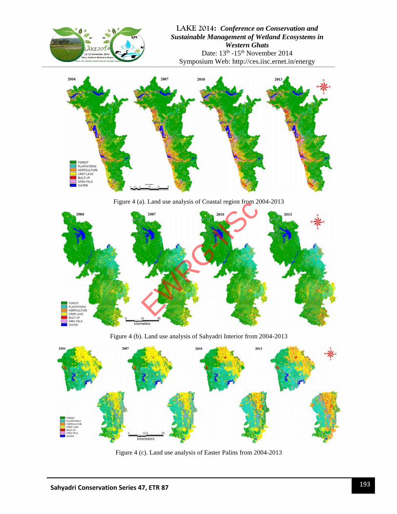
4.1. Land use analysis: The Uttara Kannadaforests are rich in biological diversity andpeople depend on the forests for a variety ofproducts. The pressure for forest basedresources from the people like palms, bamboograins and shoots, fruits like Mangifera,Artocarpus, Garcinia, Phyllanthus emblica,Syzygium cumini, pepper, cinnamon, honey,and mushroom. Apart from edible resourcesthey are also extracting thatching, basket- andmat-weaving materials, fibers, medicinalplants, etc. These non-timber products will beexported all over the world, the recent timehuge trade business is observed which iscreating more disturbances due to largeexploitation rather than controlled collection.The temporal land use analysis was carried outfor the year 2004, 2007, 2010, and 2013 acrossthe three agro climatic zones are depicted inFigure 4 (a, b, c) and category wise changesare listed in Table 3. The coastal zone showsthe loss of forest cover from 66.55 to 59.06%

by 2013 due to greater increase in populationand land conversion. The area underhorticulture has increased from 6.01 to 8.79 %by intensive plantation of Cocos nucifera,Areca Catechu. The built-up area hasincreased from 3.85% (2004) to 4.49% (2013).These abrupt changes are mainly due toanthropogenic activities than natural processes.The forests have undergone tremendoustransformation due to increase indevelopmental activities (Nuclear powerproject, Project Seabird, major industries, etc.)and inappropriate management has led toimbalances in the ecosystem, evident fromseries of landslides in the coastal taluks.

The land use analysis of Sahyadri region (Figure 4(b)) highlights the agriculture and deforestationtook place at the expense of the irreversible lossesof forest cover have led to the losses of vitalecosystem goods and services ranging frombiodiversity to regulation of hydrological cycleused to be provided for the region. Among the

EWRG-II

Sc





three zones Sahyadri Interior region has moreintact forests due to elevation. The forest cover hasreduced from 65.98 to 60.61% by 2013 due toincrease in plantation activities and horticulture.The Supa taluk shows least changes in its land usedue to less population and major area is underAnshi-Dandeli tiger reserve (ADTR). The Sirsi,Siddapur taluks has major contribution due tointensification of horticulture, Yellapura region hasmajor monoculture plantaions. It is also evidentthat the increase in plantation of exotic speciessuch as Acacia auriculiformis, Casuarinaequisetifolia, Eucalyptus spp., and Tectona grandisare led to removal of primeval forest cover. Theother driving forces are observed as market basedagriculture and fuel wood requirement whichpressurising the forests of nearby villages. Tocompensate the pressure there is intensifiedplantation activities took place. This is also one ofthe causal factors for loosing natural forest cover.The land use analysis of Plains (Figure 4 (c))

articulates the temporal changes in the region dueto human induced pressure. The region has leftwith only 15.17% forest cover by 2013 due tointensive plantation activities to meet raw materialrequirements for West coast paper mill, Dandeliwithin Haliyal taluk, even though this region isrich in faunal diversity. The plantations constitute39.82% is considered more important source ofrevenue having higher pressure in terms of woodand agriculture intensification. The region hasbecome more and more dynamic and leading tointensified land use changes and becoming rainshadow area. The built-up area has increased from2.92 to 6.26% due to population growth. The fielddata and Google earth data sets are used foranalysing accuracy of classification and theaccuracy assessment was included in Table 4. Thisapproach has provided us more consistent results.The areas of each category are also verified withavailable administrative reports, statisticaldepartment data and forest division annual reports.

Zone Coastal region Sahyadri Interior PlainsCategory (%) 2004 2007 2010 2013 2004 2007 2010 2013 2004 2007 2010 2013

Forest 66.55 63.95 63.08 59.06 65.98 63.84 62.86 60.61 27.35 23.82 20.08 15.17

Plantations 5.67 5.80 6.35 9.04 15.00 15.87 16.01 17.29 34.28 35.46 38.51 39.82

Horticulture 6.01 7.29 7.73 8.79 3.80 3.90 4.42 4.10 1.33 1.37 1.64 1.34

Crop land 10.94 10.70 10.43 10.84 10.18 10.69 10.69 10.99 29.23 30.56 30.38 28.50Built-up 3.85 4.36 4.35 4.49 1.13 1.25 1.44 2.12 2.92 3.11 4.00 6.26

Open fields 3.02 4.29 4.34 4.23 1.29 1.73 1.82 2.40 3.06 3.94 3.55 7.16

Water 3.95 3.61 3.72 3.55 2.61 2.71 2.76 2.49 1.83 1.73 1.84 1.75Total area (Ha) 335561.32 541195.99 152505.69

Table 3: Land use analysis from 2004-2013.

EWRG-II

Sc





Figure 4 (a). Land use analysis of Coastal region from 2004-2013

Figure 4 (b). Land use analysis of Sahyadri Interior from 2004-2013

Figure 4 (c). Land use analysis of Easter Palins from 2004-2013

EWRG-II

Sc





Year 2004 2007 2010 2013Categories PA UA PA UA PA UA PA UA

Forest 87.44 95.73 97.85 97.83 99.69 96.02 98.56 93.31Plantations 92.60 76.51 84.69 84.71 60.09 95.37 98.27 91.32

Horticulture 98.01 76.49 79.30 79.26 57.91 75.69 86.13 37.46Crop 92.50 85.96 86.67 86.69 71.46 95.02 79.66 81.85

Built-up 48.68 73.79 65.91 66.09 93.17 65.61 60.04 96.50Open fields 68.22 68.30 62.75 62.91 89.40 83.13 93.97 89.74

Water 80.29 89.49 92.71 93.06 78.85 94.57 96.94 97.19Kappa 0.82 0.85 0.85 0.86

Overall Accuracy 88.67 91.67 92.6 91.02

Table 4: Accuracy assement of the land use analysis.

4.2. Visualisation and prediction: The landscapevisualisation and future land use transitionswith respect to each land use category werecalculated to predict land use for 2010, usingMarkov chain process based on 2004 and 2007land use and CA loop time of 3 years, and wascontinued for 2013 by using 2007, 2010 landuse maps. With the knowledge of 2004-2007,2007-2010 and 2010-2013 for the year 2016,2019 and 2022 were predicted under differentconditions (i.e. transition rules, iterationnumbers). This prediction has been doneconsidering water bodies as a constraint andassumed to remain constant over all timeframes. The validation results showed inTable 3& 7 across the zones provides a verygood agreement between the actual andpredicted maps of 2010, 2013. The accuracy ofagreement between actual land use andpredicted land use were shown in Table 5 withkappa values. The Kappa-standard index ofoptimum point as well as Kappa-location indexwas computed shows a significant correlationbetween the simulated and the actual maps.

The simulated land use (Table 6, Figure 5 (a, b, c))shows likely increase in built-up area and loss inforest cover across three regions at three year timeinterval. The process of urbanization is observed tobe high in the areas near project Sea bird, Kaigapower house and the national/state highways in thecoastal zone. The analysis highlighted the declineof forest cover from 62.24 (2010) to 48.90%

(2022) with increase in monoculture plantationsfrom 6.59% to 10.29%. The natural vegetation isbeing replaced by the plantation activities in recenttime also indicates their further growth in futureyears. The coasta taluks has witnessed changeswithin and in the neighbourhood due to theintroduction of major developmental projects thathas led to rapid land conversion. The built-up areashows an greater increase from 4.81 to 9.30 % andarea under horticulture will reach to 8.24 to 13.13% by 2022. The adverse effects of ad-hocapproaches in the developmental activities haveled to landslides, higher erosion of top soil, etc..The Sahyri Interior region also expressing sametrend in Sirsi, Siddapur, Yellapura taluks exceptSupa. The area under built-up cover will reach2.00 to 6.47% and horticultre will be 5.59% by2022. The natural forest cover will be lost from62.6 (2010) to 52.28 % (2022) and monocultureplantations will increase from16.16 (2010) to19.31% (2022). The Sirsi town, Siddapur,Yellapura town and its suburban regions willexpereience land coversion for built-up area. Thepredicted maps of Plain region stating highergrowth in the built-up cover from 5.67 to 18.36%due to existing cover and increase in population.The cropland intensification also witnessed near bymajor reservoirs and huge lakes of Plainer regions.This necessitates comprehensive land usemanagement focusing on restoration of ecosystemsto mitigate the impacts further. Analysis andcomparison of the simulated and actual land-use

EWRG-II

Sc





maps of 2022 reveal that the CA–Markov modelhas provided insights in terms of changequantification and continuous-space changemodelling. The CA-MARKOV model is mainlyconstructed as a linear presumption of the Markovmodel. The entire ecological and economic systemis not a simple linear model and is instead complexand large, this model does not consider anyenvironmental and socio-economic variables and

acts on the probable amount and location ofchange that are obtained through a Markov Chainexecution. Recently, multi-agent models havebeen developed to simulate land conversionsthrough considering the behaviours of the existingindividuals, as well as other actors. So, accountinghuman’s perception, other biophysical drivers willdefinitely increases the precision of prediction.

Zone Coastal zone Sahyadri Interior PlainsIndex Projected 2010 Projected 2013 Projected 2010 Projected 2013 Projected 2010 Projected 2013Kno 0.86 0.92 0.89 0.9 0.88 0.92

Klocation 0.84 0.91 0.87 0.86 0.86 0.93Kstandard 0.82 0.88 0.83 0.84 0.83 0.89

Table 5: Validation of actual and predicted with Kappa

Zone Coastal region Sahyadri InteriorCategory (Ha) P 2010 P 2013 P 2016 P 2019 P 2022 P 2010 P 2013 P 2016 P 2019 P 2022

Forest 62.24 57.24 55.03 51.76 48.90 62.60 60.86 57.32 54.33 52.28Plantations 6.59 9.25 9.68 9.96 10.29 16.16 17.45 18.89 18.96 19.31

Horticulture 8.24 8.98 11.62 12.63 13.13 4.44 4.80 4.70 5.38 5.59Crop land 10.22 11.14 10.23 10.23 10.14 10.55 10.64 10.40 11.25 11.46Built-up 4.81 5.02 5.48 7.55 9.30 2.00 1.78 3.81 5.19 6.47

Open land 4.29 4.65 4.53 4.69 4.94 1.73 1.86 2.40 2.40 2.40Water 3.61 3.72 3.44 3.17 3.30 2.53 2.62 2.49 2.49 2.49Zone Plains

Category P 2010 P 2013 P 2016 P 2019 P 2022Forest 20.33 14.58 11.81 10.72 9.48

Plantations 39.16 40.25 38.64 34.14 30.17Horticulture 2.02 2.55 1.40 1.95 2.09

Crop land 27.11 30.00 30.94 30.55 30.94Built-up 5.67 7.19 10.87 16.32 18.36

Open fields 3.97 3.57 4.57 4.57 7.21Water 1.75 1.86 1.76 1.76 1.76

Table 6: Land use analysis for predicted 2010-2022. (*P - Projected)

EWRG-II

Sc





Figure 5 (a): Projected Land use of Coastal region from 2013-2022.

Figure 5 (b): Projected Land use of Sahyadri Interior from 2013-2022.

Figure 5 (c): Projected Land use of Plains region from 2013-2022.

EWRG-II

Sc





CONCLUSION:

LULC analysis indicates the human andbiophysical forces are responsible for landscapecomposition and configuration. The integratedmodelling framework presented has potential innatural resource planning and management and inassessing of the effects of policies on landdevelopment, land cover. The analysis highlightedthe decline of forest cover in coastal zone from62.24 (2010) to 48.90% (2022) with increase inmonoculture plantations from 6.59% to 10.29%and built-up area from 4.81 to 9.30%. The naturalforest cover decreases in Sahyadri region from62.6 (2010) to 52.28 % (2022) and percentage ofmonoculture plantations increase from 16.16

(2010) to 19.31% (2022). The Sirsi town,Siddapur, Yellapura town and its suburban regionswill experience land conversion for built-up area.The Plain region is stating higher growth in thebuilt-up cover from 5.67 to 18.36% due to existingcover and increase in population. The land usechanges across zones are varying over spatiotemporal scale, the coastal region, plains havehigher transition as compared to Sahyadri region.The present work helps planning authorities anddecision makers to articulate policies andprogrammes to maintain a sustainable balancedecosystem or to mitigate the devastatingconsequences of severe land use changes.

ACKNOWLEDGEMENT:

We are grateful to Ministry of Environment &Forest, Ministry of Science and Technology,Government of India, Karnataka BiodiversityBoard, Western Ghats Task Force, Government ofKarnataka and Indian Institute of Science for the

financial and infrastructure support. We thank MrVinay, CES, IISc, for providing useful inputs inmodelling and analysis of this work. We also thankUSGS and NRSC for providing RS data.

REFERENCES

1. Armesto, J., Smith-Ramírez, C., Carmona, M., Celis-Diez, J., Díaz, I., Gaxiola, A., Gutierrez, A., Nú˜nez-Avila, M., Pérez, C., Rozzi,R., 2009. Old-growth temperate rain forests of South America: conservation, plant-animal interactions, and baseline biogeochemicalprocesses. Old-growth forests: function, fate and value. In: Wirth, C., Gleixner, G., Heimann, M. (Eds.), Ecological Studies, vol. 207.Springer, New York, Berlin, Heidelberg, 367–390.

2. Arsanjani, J.J., Helbich, M., Kainz, W., and Darvishi, A., 2013. Integration of logistic regression, Markov chain and cellular automatamodels to simulate urban expansion - the case of Tehran. International Journal of Applied Earth Observation and.Geoinformation, 21,265-275.

3. Batty, Michael, Jake DeSyllas, and Elspeth Duxbury. 2003. The discrete dynamics of small-scale spatial events: agent-based models ofmobility in carnivals and street parades. International Journal of Geographical Information Science, 17 (7), 673-697.

4. Bell, S., 2001. Landscape pattern, perception and visualisation in the visual management of forests. Landscape and Urban planning,54(1), 201-211.

5. Bharath Setturu and Ramachandra. T.V., 2012. Landscape dynamics of Uttara Kannada district, Proceedings of the LAKE 2012:National Conference on Conservation and Management of Wetland Ecosystems, 06th - 09th November 2012, School of EnvironmentalSciences, Mahatma Gandhi University, Kottayam, Kerala, pp. 1-13.

6. Cheong, So-Min., Brown, D., Kok, K., and López-Carr, D., 2012. Mixed Methods in Land Change Research: Towards Integration.Trans.Inst. Br. Geogr. 37, 8–12.

7. Deng, X.Z., 2011. Modeling the dynamics and consequences of land system change. Beijing: Higher Education Press.8. FAO, 2006. Global planted forests thematic study: results and analysis, by A. Del Lungo, J. Ball and J. Carle. Planted Forests and

Trees Working Paper 38.9. Hansen, M.C., Potapov, P.V., Moore, R., Hancher, M., Turubanova, S.A., Tyukavina, A., Thau, D., Stehman, S.V., Goetz, S.J.,

Loveland, T. R., Kommareddy, A., Egorov, A., Chini, L., Justice C.O., and Townshend, J.R.G., 2013. High-Resolution Global Maps of21st Century Forest Cover Change Science, 342 (6160), 850-853.

10. Haase, D., and Schwarz, N., 2009. Simulation models on human-nature interactions in urban landscapes – a review including systemdynamics, cellular automata and agent-based approaches. Living Reviews in Landscape Research, 3, 2.

11. Houet T., and Hubert-Moy L., 2006. Modelling and Projecting Land-Use and Land-Cover Changes with a Cellular Automaton inConsidering Landscape Trajectories: An Improvement for Simulation of Plausible Future States, EARSeL eProceedings, 5, 63–76.

EWRG-II

Sc





12. Kamusoko C., Aniya M., Adi B., and Manjoro M., 2009. Rural sustainability under threat in Zimbabwe – Simulation of future landuse/cover changes in the Bindura district based on the Markov-cellular automata model, Applied Geography, 1.

13. Kanowski, J., Catteral, C.P., and Wardell-Johnson, G.W., 2005. Consequence of broad scale timber plantations for biodiversity incleared rainforest landscape of tropical and subtropical Australia, Forest Ecology and Management, 208, 359–372.

14. Lillesand, T.M., and Keifer, R.W., 1987. Remote sensing and Image interpretation, John Willey and Sons, New York.15. Macedo, R.D., de Almeida, C.M., dos Santos, J.R., and Rudorff, B.F.T., 2013. Spatial dynamic modeling of land cover and land use

change associated with the sugarcane expansion. Bol. Cienc. Geod. 19, 313–337.16. Maguire, D., Batty, M., and Goodchild, M., 2005.GIS, spatial analysis, and modelling. Redlands, CA: Esri Press.17. Moreno, N., Wang, F., and Marceau, D.J., 2009. Implementation of a dynamic neighbourhood in a land-use vector-based cellular

automata model. Computers, Environment and Urban Systems, 33 (1), 44–54.18. Nole, G., Rosa L., and Beniamino M., 2013. Applying spatial autocorrelation techniques to multi-temporal satellite data for measuring

urban sprawl. Int. J. Environ. Protect 3 (7), 11-21.19. Pontius Jr, R.G., Shusas, E., and McEachern, M., 2004. Detecting important categorical land changes while accounting for persistence.

Agriculture, Ecosystems and Environment, 101 (2–3), 251–268.20. Pontius, R.G.J., and Malanson, J., 2005. Comparison of the structure and accuracy of two land change models. Int. J. Geogr. Inf. Sci.

19, 243-265.21. Ramachandra T.V., and Shruthi, B.V., 2007. Spatial mapping of renewable energy potential, Renewable and Sustainable Energy

Reviews, 11(7), 1460-1480.22. Ramachandra, T.V., Setturu Bharath and Aithal Bharath., 2014. Spatio-temporal dynamics along the terrain gradient of diverse

landscape, Journal of Environmental Engineering and Landscape Management, 22:1, pp. 50-63.,doi:http://dx.doi.org/10.3846/16486897.2013.808639.

23. Riccioli, F., EI Asmar, T., EI Asmar, J.P., and Fratini, R., 2013. Use of cellular automata in the study of variables involved in land usechanges. Environ. Monit. Assess. 185, 5361–5374.

24. Tattoni, C., Ciolli, M., and Ferretti, F., 2011. The fate of priority areas for conservation in protected areas: A fine-scale Markov chainapproach. Environ. Manage. 47, 263–278.

25. Tian, G.J., Ouyang, Y., Quan, Q.A., and Wu, J.G., 2011. Simulating spatiotemporal dynamics of urbanization with multi-agent systems– A case study of the Phoenix metropolitan region, USA. Ecol. Model. 222, 1129–1138.

26. Turner II, B., 2009. Land change science. In: R. Kitchen, and N. Thrift, eds. International Encyclopedia of Human Geography. Oxford:Elsevier, 107–111.

27. Walsh, S.J., Messina, J.P., Mena, C.F., Malanson, G.P., and Page, P.H., 2008. Complexity theory, spatial simulation models, and landuse dynamics in the Northern Ecuadorian Amazon. GeoForum 39(2), 867-878.

28. Wimberly, M.C., and Ohmann, J.L., 2004. A multi-scale assessment of human and environmental constraints on forest land coverchange on the Oregon (USA) coast range. Landscape Ecology 19(6), 631-646.

29. Wu, Y.Z., Zhang, X.L., and Shen, L.Y., 2011. The impact of urbanization policy on land use change: a scenario analysis. Cities 28,147–159.

30. Yang, X., Zheng, X.Q., and Lv, L.N., 2012. A spatiotemporal model of land use change based on ant colony optimization, Markovchain and cellular automata. Ecol. Model. 233, 11–19.EW

RG-IISc

visualization of forest transitions in uttara kannadawgbis.ces.iisc.ernet.in/energy/lake2014/... ·...

Documents