viv kendon - cirm-math.fr

How to compute using

quantum walks

PhD students:

James Morley (UCL→ CountingLabs)

Adam Callison (Imperial)

Jemma Bennett (Durham)

Stephanie Foulds (Durham)

+ many UG project students

also at Durham:

Nick Chancellor (Durham)

(UKRI Innovation Fellow)

Jie Chen (Durham)

Laur Nita (Durham)

Viv Kendon

Collaborators:

Dom Horsman

(Grenoble)

Susan Stepney (York)

JQC & QLM

Physics Dept

Durham University

[email protected]

Quantum Simulation and Quantum Walks

CIRM 20th January 2020

January 19, 2020 QSQW - CIRM 20.1.2020

Overview

• modeling vs simulation?

• abstraction/representation framework

• solving classical problems with quantum walks

• searching and spin glasses

• universal quantum walk computing

• summary and outlook

��

��

��

��

��

��

��

��

��

��

��

��

��

��

��

��

��

��

64321−1−2−3−4−5−6−7−8−9 8 90 75

+ + + + + + + + + + + + + + + + + + + + + + + + + + + + + + + + + + + + + + + +2/34


numerical simulation...

⋆ we simulate mathematical models, not physical systems:

Mathematical Model

Numerical simulationAnalytical calculations Experiments

Model

COMPARE

Revise

computational physics tests our models when can’t calculate analytically...

+ + + + + + + + + + + + + + + + + + + + + + + + + + + + + + + + + + + + + + + +3/34


representation relation in physics:

abstract

physical

e−

ψ : i~∂ψ

∂t= Hψ

RT

spaces of abstract and physical objects (here, an electron and a wave-function)

with a representation relation (modelling) RT mediating between the spaces

R is theory dependent, so write RT for theory T

⋆ could represent electron as point charge if doing electrostatics . . .

+ + + + + + + + + + + + + + + + + + + + + + + + + + + + + + + + + + + + + + + +4/34


science

abstract

physical

p

mp

RT

m′p

CT (mp)

p′time goes by

H(p)

mp′

RT

ε

– physical system p evolves under H(p) to p′

– theory mp calculated CT (mp) to obtain m′p

– “good” theory agrees with observation to within ε : |m′p − mp′ | < ε

+ + + + + + + + + + + + + + + + + + + + + + + + + + + + + + + + + + + + + + + +5/34


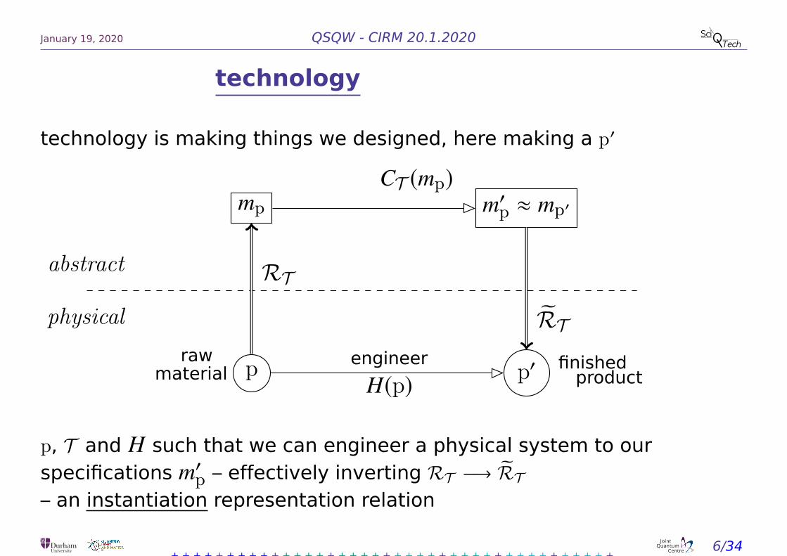
technology

technology is making things we designed, here making a p′

abstract

physical

praw

material

mp

RT

m′p ≈ mp′

CT (mp)

p′ finishedproduct

engineer

H(p)

RT

p, T and H such that we can engineer a physical system to our

specifications m′p – effectively inverting RT −→ RT

– an instantiation representation relation

+ + + + + + + + + + + + + + + + + + + + + + + + + + + + + + + + + + + + + + + +6/34


computing

among many things, we engineer computers

abstract

physical

p

mp

RT

m′p ≈ mp′

c

encode

c′

decode

p′program runs

H(p)

RT

computing: use a physical computer p to calculate abstract problem c

encode c into model mp, instantiate RT into p, run, decode output

+ + + + + + + + + + + + + + + + + + + + + + + + + + + + + + + + + + + + + + + +7/34


requirements for computing

computing is a high level process...abstract

physical

p

mp

RT

m′p ≈ mp′

c

encode

c′

decode

p′program runs

H(p)

RT

• computations have outputs (else can replace computer with brick...)

• representational entity (“owns” the computation)

[Stepney/VK “The role of the representational entity...” 219–231 UCNC 2019 & Nat. Comp. 2020]

abstract is instantiated in the representational entity

(does not need to be human – Horsman/VK/Stepney/Young Abstraction and representation in living

organisms: when does a biological system compute? in: Representation and reality: Humans, Animals

and Machines. Gordana Dodig-Crnkovic and Raffaela Giovagnoli, Editors. Springer 2016)

+ + + + + + + + + + + + + + + + + + + + + + + + + + + + + + + + + + + + + + + +8/34


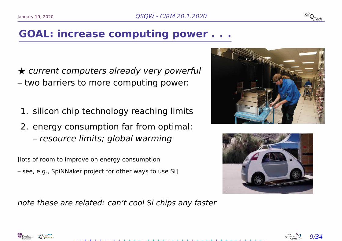
GOAL: increase computing power . . .

⋆ current computers already very powerful

– two barriers to more computing power:

1. silicon chip technology reaching limits

2. energy consumption far from optimal:

– resource limits; global warming

[lots of room to improve on energy consumption

– see, e.g., SpiNNaker project for other ways to use Si]

note these are related: can’t cool Si chips any faster

+ + + + + + + + + + + + + + + + + + + + + + + + + + + + + + + + + + + + + + + +9/34


beyond silicon . . .

quantum: IBM 5 qubit

BZ reaction chemical reservoir computer

rat neuron on silicon encoding for DNA computer

⋆ future computing is diversifying ⋆

⇒ need to co-design algorithms with hardware ⇐

+ + + + + + + + + + + + + + + + + + + + + + + + + + + + + + + + + + + + + + + +10/34


hybrid computers . . .

practice: co-processors: unconventional: control + substrate:

conventional:

• graphics cards

• ASIC application-specific integrated circuit

• FPGA field-programmable gate array

• quantum

• NMR

• reservoir

• slime mould

⋆ hybrid computational systems are the norm ⋆

theory: single paradigm:

• classical – Turing Machine

• analog – Shannon’s GPAC

• quantum – gate model, QTM, CV, MBQC, QW, AQC, . . .

• linear optics (Bosons) [Aaronson/Arkhipov STOC 2011 ECCC TRI-10 170]

+ + + + + + + + + + + + + + + + + + + + + + + + + + + + + + + + + + + + + + + +11/34


quantum computing

input −→ encode −→ |ψin〉 −→ U −→ |ψout〉 −→ decode −→ result

U is unitary evolution (or more generally, open system/environment)

– can be gate sequence , or engineer Hamiltonian H(t) such that

|ψout〉 = T exp{−i/~∫

dt H(t)} |ψin〉

⋆ covers most of quantum information processing . . .

. . . including communications, where aim is result=input

encode – arbitrary choices:

using spin-down |↓〉 ≡ 0 instead of spin-up |↑〉 ≡ 0 makes no difference

→ provided encode and decode done consistently

+ + + + + + + + + + + + + + + + + + + + + + + + + + + + + + + + + + + + + + + +12/34


quantum information processing

quantum information is built on the idea that:

quantum logic allows greater EFFICIENCY than classical logic

classical quantum

bits, 0 or 1 qubits, α |0〉 + β |1〉yes or no, binary decisions yes and no, superpositions

HEADS or TAILS, random numbers random measurement outcomes

⇒ quantum gives different computation from classical: how different?

• computability – what can be computed?

• complexity – how efficiently can it be computed?

⇒ quantum computability is the same as classical

complexity differs: some problems can be computed more EFFICIENTLY

+ + + + + + + + + + + + + + + + + + + + + + + + + + + + + + + + + + + + + + + +13/34


quantum advantage?

how to translate quantum logic into better computing devices?

depends on definition of EFFICIENCY

• in theory: polynomial scaling with system size

• in practice: produces answers on human timescales

roughly speaking:

quadratic speed up exploits quantum coherence, interference effects

exponential speed up exploits parallelism in quantum superposition

⋆ comparison of real physical devices, not of mathematical theories

⇒ complexity theory alone won’t tell you whether useful in practice

��

��

��

��

��

��

��

��

��

��

��

��

��

��

��

��

��

��

��

��

+ + + + + + + + + + + + + + + + + + + + + + + + + + + + + + + + + + + + + + + +14/34


encoding matters . . .

. . . it determines the physical resources required:

Number Unary Binary

0 0

1 • 1

2 •• 10

3 • • • 11

4 • • •• 100

· · · · · · · · ·2x4 • • •• 1000

=8 • • ••· · · · · · · · ·

N N × • log2 N bits

Read out:

Unary: measurements with N

outcomes

Binary: log2 N measurements

with 2 outcomes each

−→ exponentially better for precision

[Ekert & Jozsa PTRSA 356 1769-82 (1998)]

−→ exponential reduction in memory

[does not have to be binary: Blume-Kohout, Caves,

I. Deutsch, Found. Phys. 32 1641-1670 (2002)]

⋆ floating point: 0.1234567 × 1089 even more efficient, trade precision/memory ⋆

+ + + + + + + + + + + + + + + + + + + + + + + + + + + + + + + + + + + + + + + +15/34


encoding problems into qubit Hamiltonians

+ computational basis state | j〉 = |q0q1 . . . qk . . . qn−1〉 with qk ∈ {0,1}+ superposition of all basis states:

|ψ0〉 = 2−n/22n−1∑j=0

| j〉 = (|0〉 + |1〉)⊗n

encode problem into n-qubit Hamiltonian Hp

such that solution is lowest energy state (ground state)

example: find state |m〉 then Hp = 11 − |m〉〈m|

example: three qubits, exactly one must be |1〉

Hp = (11 − Z1 − Z2 − Z3)2

Pauli-Z operator: Z |0〉 = |0〉 and Z |1〉 = − |1〉

Z =©«1 0

0 −1ª®¬

X =©«0 1

1 0

ª®¬

+ + + + + + + + + + + + + + + + + + + + + + + + + + + + + + + + + + + + + + + +16/34


continuous-time quantum computing

family of computational models:

• discrete – qubits for

efficient encoding

• continuous time evolution

with engineered Hamiltonian

• coupling to low temp bath –

open system effects

cooling

QA

QW AQCunitary

cold open

m

noise

(high

exploits natural properties of quantum systems

+ + + + + + + + + + + + + + + + + + + + + + + + + + + + + + + + + + + + + + + +17/34


adiabatic quantum computing

given Hp [Farhi et al, quant-ph/0001106]

initialise in ground state��ψinit⟩ of simpler Hamiltonian H0 – easy to prepare –

transform adiabatically:

H(t) = [1 − s(t)]H0 + s(t)Hp

with annealing parameter s(t = 0) = 0 and s(t = t f ) = 1

s(t) monotonically increasing, function of size of problem space N = 2n and the

accuracy parameter ǫ determined by adiabatic condition,

��⟨ dHdt⟩1,0

��(E1 − E0)2

≡ ǫ ≪ 1, (1)

0 and 1 refer to the ground and excited states, and��⟨ dHdt

⟩1,0

�� ≡ 〈E1 | dHdt |E0〉

closer ǫ is to zero – the more completely the system will stay in the ground state

and the longer the computation will take

+ + + + + + + + + + + + + + + + + + + + + + + + + + + + + + + + + + + + + + + +18/34


continuous time quantum walk

[Farhi & Gutmann, PRA 58, 915-928 (1998); exponential speed up: Childs et al STOC

2003; universal for QC: Childs PRL 102, 180501 2009]

A – adjacency matrix of graph (Ajk = 1 iff ∃ an edge between sites j and k)

Laplacian: L = A −D, where D is diagonal matrix Dj j = deg( j), the degree of site j

Laplacian L = A −D, of graph [irrelevant global phase for regular graphs]

Hamiltonian of the quantum walk: Hw = −γL

γ = transition rate (prob of moving to connected site per unit time)

quantum walk is ψ(t) = exp{−iHwt}ψ(0) then measure at time t = t f

−9 −8 −7 −6 −5 −4 −3 −2 −1 1 2 3 4 5 6 8 90 7

+ + + + + + + + + + + + + + + + + + + + + + + + + + + + + + + + + + + + + + + +19/34


encoded hypercubes for quantum walks

n qubits encode 2n vertices:

for a hypercube graph, Hh = γ(n11 −∑j Xj

)

where j is the qubit label: j = 0 . . . n − 1

Pauli-X operator Xj

bit-flips qubit j 0↔ 1

−→ this moves the position of the quantum

walker along an edge of the hypercube

N = 8

n = 3

100

110

101

111

000

010

001

011

N = 4

n = 2

00

01

10

11

N = 2

n = 1

0 1

+ + + + + + + + + + + + + + + + + + + + + + + + + + + + + + + + + + + + + + + +20/34


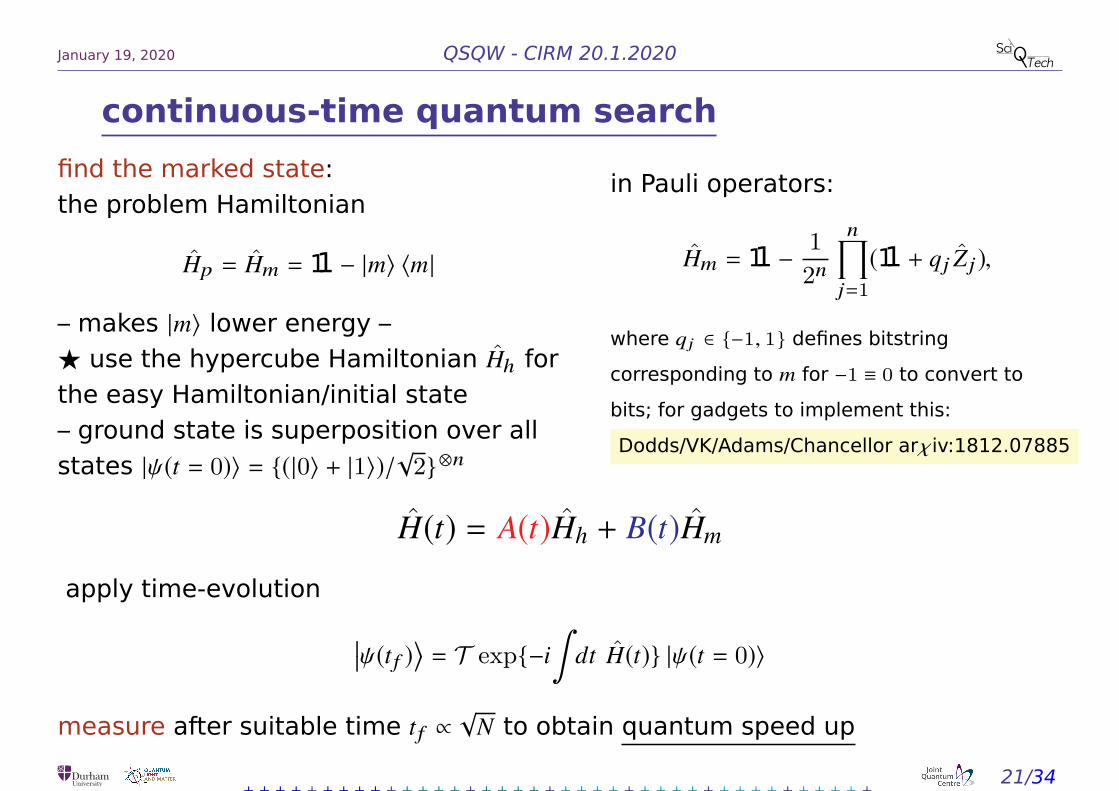
continuous-time quantum search

find the marked state:

the problem Hamiltonian

Hp = Hm = 11 − |m〉〈m|

– makes |m〉 lower energy –

⋆ use the hypercube Hamiltonian Hh for

the easy Hamiltonian/initial state

– ground state is superposition over all

states |ψ(t = 0)〉 = {(|0〉 + |1〉)/√2}⊗n

in Pauli operators:

Hm = 11 −1

2n

n∏j=1

(11 + qj Z j ),

where qj ∈ {−1, 1} defines bitstringcorresponding to m for −1 ≡ 0 to convert to

bits; for gadgets to implement this:

Dodds/VK/Adams/Chancellor arχiv:1812.07885

H(t) = A(t)Hh + B(t)Hm

apply time-evolution

��ψ(t f )⟩ = T exp{−i

∫dt H(t)} |ψ(t = 0)〉

measure after suitable time t f ∝√

N to obtain quantum speed up

+ + + + + + + + + + + + + + + + + + + + + + + + + + + + + + + + + + + + + + + +21/34


hybrid continuous-time quantum search algorithms

interpolate between

QW (α = 0) andAQC (α = 1)

H(α, t) = A(α, t)Hh + B(α, t)Hm

HQW = γHh + Hm

HAQC = [1 − s(t)]Hh + s(t)Hm

→ need γ and s(t) . . .

[James Morley’s work (UCL CDT)

PRA 99, 022339 (2019)

arχiv:1709.00371]

+ + + + + + + + + + + + + + + + + + + + + + + + + + + + + + + + + + + + + + + +22/34


single avoided crossing model

continuous-time quantum seach algorithms all solved analytically

– for large N limit reduces to a 2-dim subspace (single qubit) – for AQC

H(AC)(s) = (1 − s)H(AC)0

+ sH(AC)p

= (1 − s){1

2(11 + Z) − gmin X

}+ s

1

2(11 − Z)

with gmin = N−1/2 solving the eigensystem gives

E1 − E0 = g(AC)(s) = {(1 − 2s)2 + 4g2

min(1 − s)2}

1

2

apply method of Roland+Cerf (2002) to obtain optimal s(t) as solution of

ds

dt=

ǫ[g(AC)(s)]2��⟨dHACds

⟩0,1

��= (1 − 2s)2 + 4g2

min(1 − s)2

in limit gmin ≪ 1

s(t) ≃ 1

2

{1 − gmin cot

[gmin(2ǫ t + 1)

]}+ + + + + + + + + + + + + + + + + + + + + + + + + + + + + + + + + + + + + + + +

23/34


single avoided crossing model

for quantum walk, γ ≡ s = 1/2 and model reduces to Rabi flops

H(γ) = 1

2(11 − gmin X)

interpolate between QW (α = 0) and AQC (α = 1) where β = 1/(1 + γ)

H(α, t) = A(α, t)Hh + B(α, t)Hm

HQW = γHh + Hm

HAQC = [1 − s(t)]Hh + s(t)Hm

A(α, t) = 1 − s(τ)α + (1 − α) (1−s(t))(1−β)

B(α, t) = s(t)α + (1 − α) s(t)

β

[James Morley’s work (UCL CDT)]

+ + + + + + + + + + + + + + + + + + + + + + + + + + + + + + + + + + + + + + + +24/34


more realistic problems

Sherrington Kirkpatrick spin glasses: frustrated spin systems

⋆ NP-hard for finding ground state i.e., expect polynomial speed up

⋆ more like realistic hard optimisation problems

Hp = −n=1∑j=0

n−1∑k=j+1

Jjk + Jk j

2Z j Zk −

n=1∑j=0

hj Z j

Jjk, hj drawn from Gaussian distributions with mean = 0 (hardest)

• AQC can find ground states faster than guessing

[e.g., Martin-Mayor/Hen Sci Rep 5, 15324 (2015); arXiv:1502.02494]

H(t) = (1 − s(t))Hw + s(t)Hp

• what about continuous-time quantum walks?

H(t) = γHw + Hp

• compare with a random energy model (REM)

+ + + + + + + + + + + + + + + + + + + + + + + + + + + + + + + + + + + + + + + +25/34


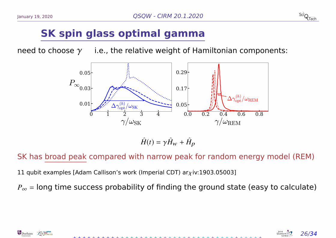
SK spin glass optimal gamma

need to choose γ i.e., the relative weight of Hamiltonian components:

0 1 2 3 4γ/ωSK

0.01

0.03

0.05

P∞

∆γ(h)opt/ωSK0.0 0.2 0.4 0.6 0.8

γ/ωREM

0.05

0.17

0.29

∆γ(h)opt/ωREM

H(t) = γHw + Hp

SK has broad peak compared with narrow peak for random energy model (REM)

11 qubit examples [Adam Callison’s work (Imperial CDT) arχiv:1903.05003]

P∞ = long time success probability of finding the ground state (easy to calculate)

+ + + + + + + + + + + + + + + + + + + + + + + + + + + + + + + + + + + + + + + +26/34


SK spin glass QW dynamics

8 qubit example:

top: time evolution of ground state prob

bottom: time-averaged ground state prob

measure at random time to sample

time-averaged probability

P(t,∆t) = 1

∆t

∫ t+∆t

t

dtP(t)

(time scaling better than O(log N ), numerically

n0.75)

[Adam Callison (Imperial CDT) arχiv:1903.05003]

+ + + + + + + + + + + + + + + + + + + + + + + + + + + + + + + + + + + + + + + +27/34


SK spin glass results

success probability scaling for heuristic γ based on energy scales

6 8 10 12 14 16 18 20

n

2 8

2 6

2 4

2 2

P

P(0) = 2� nP�P(12.5 n� SK , 5.0 n� SK )

(average over 10,000 random instances)

don’t need to solve problem to set parameters, heuristic does well

P ∼ N−0.41 for short run times [Callison/Chancellor/Mintert/VK arχiv:1903.05003 & NJP]

cf P ∼ N−0.5 for search, i.e., ⋆ better than search ⋆

+ + + + + + + + + + + + + + + + + + + + + + + + + + + + + + + + + + + + + + + +28/34


SK spin glass structure

2 5

2 4

2 3

2 2

< P

>

SK hypercube

SK complete

sSK hypercube

REM hypercube

REMGC hypercube

5 6 7 8 9 10n

11

HSK = −n−1∑j=0

n−1∑k=j+1

Jjk + Jk j

2Z j Zk −

n−1∑j=0

hj Z j

←− need to know γ

precisely = not practical?

+ add pairwise corrs to REM

– remove corrs from SK

– remove corrs from Hw

⇒ pairwise correlations

matched with hypercube

QW Hamiltonian work best

Hh = 11 −1

n

n=1∑j=0

Xj

real problems have correlations ⋆ match problem encoding to algorithm ⋆

[Callison/Chancellor/Mintert/VK arχiv:1903.05003 & NJP]

+ + + + + + + + + + + + + + + + + + + + + + + + + + + + + + + + + + + + + + + +29/34


Quantum walks are universal for quantum computing

[Childs PRL 102 18051 arχiv:0806.1972]

[Lovett/Cooper/Everitt/Trevers/VK PRA 81 042330 arχiv:0910.1024]

...about proving can implement QW efficiently on a quantum computer

...has nothing to do with physical implementation of quantum walks

key phrase from Childs’ paper: “any sufficiently sparse graph”

i.e., graph has a description that is logarithmic in the number of sites

Childs’ results characterise which Hamiltonians are efficient to simulate

on a quantum computer [Berry et al. Comm. Math. Phys. 270 359 (2007)]

this gate model circuit:

H P

+ + + + + + + + + + + + + + + + + + + + + + + + + + + + + + + + + + + + + + + +30/34


Quantum walk gates

...becomes this quantum walk graph (thanks to Neil Lovett for figure)

H

H

H

H

exponential number of

sites is compensated

for by binary encoding

and superposition

+ + + + + + + + + + + + + + + + + + + + + + + + + + + + + + + + + + + + + + + +31/34


Multiple quantum walkers

⋆ quantum walkers that interact at the same or neighbouring sites

– like a spin lattice with many excitations delocalised over the lattice

– special case of quantum cellular automata

QCA are universal for quantum computing

– Quantum Cellular Automata overview: [Wiesner arχiv:0808.0679]

– continuous-time quantum walk construction of universal quantum computation

[Childs+Gosset+Webb Science 339, 791 2013] m walkers on L locations −→ full Hilbert

space is Lm

⋆ experiments: atoms in optical lattice [Karski et al Science 325 174 (2009)]

⋆ multiple non-interacting walkers = particle statistics:

• bosons, intermediate between classical and quantum computing

Aaronsons+ Arkhipov arχiv:1011.3245

• fermions, only two at once if start on same site – simulate with entanglement

Sansoni et al arχiv:1106.5713

+ + + + + + + + + + + + + + + + + + + + + + + + + + + + + + + + + + + + + + + +32/34


CTQW computation summary

1. quantum walks can find spin glass ground states

– quantum speed up (polynomial, better than Grover’s search)

– Callison/Chancellor/Mintert/VK arχiv:1903.05003 / NJP 21 123022 2019

2. continuous-time quantum computing for simulation and

computation

– Morley/Chancellor/Bose/VK arχiv:1709.00371 / PRA 99 022339 2019 search

3. abstraction/representation theory framework

– Horsman/Stepney/Wagner/VK Proc. Roy. Soc. A 470(2169):20140182

– Horsman/Stepney/VK Communications of the ACM 60:8 31-34 2017

– Stepney/VK “The role of the representational entity...” 219–231 UCNC 2019

��

��

��

��

��

��

��

��

��

��

��

��

��

��

��

��

��

��

64321−1−2−3−4−5−6−7−8−9 8 90 75

+ + + + + + + + + + + + + + + + + + + + + + + + + + + + + + + + + + + + + + + +33/34


what next?

• QW on more problems e.g. MAX2SAT

– (Adam Callison with Lewis Light & Puya Mirkarimi)

• adapt Ashley Montanaro’s branch and bound speed up to continous-time

– optimal algorithm for spin glass ground state problem

– (Adam Callison with Zoë Bertrand & Max Fentenstein)

• cooling/open system effects – single avoided crossing model/search problem

– (Jim Cresser & Steve Barnett (Glasgow); Parth Patel)

��

��

+ + + + + + + + + + + + + + + + + + + + + + + + + + + + + + + + + + + + + + + +34/34

viv kendon - cirm-math.fr

Documents