1

Bribe “Frequency” and Corruption in Economies

Vivekananda Mukherjee

Aparajita Roy*

Department of Economics, Jadavpur University, Kolkata 700032, India

September 2011

*Corresponding Author. E-mail: aparajita.roy1@gmail.com

Phone: +91-9831146381

The paper has benefitted from helpful discussion with Siddhartha Mitra. Usual disclaimer applies.

2

Abstract

The paper develops a theoretical model to study how size of corruption (defined as amount of revenue

generated through bribes) varies with commonly obtained data on corruption for different economies that

is “frequency” at which firms are asked for bribes. It accommodates both „high‟ and „low‟ levels of

bureaucracies which are corruptible, and finds that bribe “frequency” negatively correlates with both the

overall size of corruption and the size of „high‟ level corruption present in the economy. Therefore the

ranking of the economies based on “frequency” data may not reflect the same based on their overall size

of corruption. The model not only explains the low level of development in economies with high

“frequency” of bribery, also explains the observed independence of two levels of bureaucracies in these

economies. It draws some important policy implications for economic development and control of

corruption in economies.

Keywords: corruption, bureaucracy, bribe frequency, welfare, „kleptocracy‟

JEL Classification: D61, D73, H11

3

1. Introduction

How do we measure “corruption” in an economy? A careful study of existing literature in

economics reveals that it can be done at least in three different ways. While authors like Mookherjee and

Png (1995) take it as frequency at which a bribe incidence occurs in an economy, Shleifer and Vishny

(1993) take it as bribe rate. In a recent paper Zenger (2011) takes it as the amount of revenue generated

through bribes. Unless all of them are positively correlated with each other, it seems reasonable that when

we talk about overall size of “corruption” in economies we should take the size of bribe revenue as its

measure. However due to illegal nature of bribe transactions, the data on bribe revenue is hardly

available. The most frequently used data set on “corruption” the Corruption Perception Index (CPI) is

prepared on the basis of responses from the people to the questions which ask them either about

“prevalence” or “commonness” or “frequency” or “likelihood” of corruption1. Clearly CPI is based on the

first measure described above. In some of the cases micro-data on both frequency and bribe rates are

available like in Olken and Barron (2009) who collected data on bribes paid by the truck drivers on the

way of transporting goods in Indonesia. They relate the bribe rate to frequency with which the bribes are

asked at different checkpoints. But since they do not have the data on how the number of trucks varied

with the variation of the bribe rate we are not able to relate the “bribe rate” and “frequency” with the total

takes of bribe revenue; and thus with overall corruption of the economy. Do the data on “frequency” and

“bribe rate” positively correlate with the overall size of corruption? In this paper we attempt to find a

theoretical answer to this question.

We construct a model of an economy which has corruption both at the high and low levels of the

bureaucracy. A „high‟ level bureaucrat takes bribe from competing firms to award a monopoly license for

operating in a particular industry to one of them. The firms rewarded with the licenses to operate in

different industries have to bribe the „low‟ level officials to access essential inputs required for

production. A „low‟ level official enjoys monopoly power to facilitate access to the essential inputs to

1 See Lambsdorff (2007) for details of construction of CPI.

4

firms and charges a mark-up over the official price of the input. Thus the number of independent „low‟

level officials stands for bribe “frequency” in our model2. The mark-up (the bribe rate) and the overall

size of corruption (the bribe revenue) are endogenously determined from the model. We find that the

“frequency” and the “bribe rate” positively correlate with each other as predicted by Shleifer and Vishny

(1993) before and as empirically verified by Olken and Barron (2009) later. But, the overall size of

corruption in the economy inversely varies with them. So we conclude all other things remaining the

same, ranking of the economies according to bribe “frequency” as practiced by CPI may not reflect the

ranking of the economies according to their overall size of corruption. Our model also predicts that the

„high‟ level corruption in an economy must be falling with bribe “frequency”. We also show that in

economies with higher “frequency” of bribes, lower overall size of corruption and lower welfare level

coexist with each other.

The results we have outlined above crucially depend on the assumption that the independent

„low‟ level bureaucrats exist in economies and they behave like monopolies over the supply of respective

essential inputs. How realistic is this assumption? Given the fact that the monopoly behavior of the

independent „low‟ level officials reduce the bribe revenue collected by the „high‟ level official, does not

the „high‟ level official try to strike a coalition with the „low‟ level officials such that they are adequately

compensated for behaving competitively? Earlier Kahana and Nitzan (2002) solved an organizational

design problem under similar situation and concluded that the optimum bureaucratic friction at the „low‟

level should reduce to zero. In this paper we consider a mechanism similar to the conjecture by Moe

(1984) through which a high level “career” bureaucrat attempts to control its subordinates and finds that

such a mechanism fails to take off. This explains why we observe both „high‟ and „low‟ level bureaucrats,

who are bribe-seeking, in a large number of economies. In support of existence of independent „low‟ level

bureaucrats in reality De Soto (2000) reports obtaining legal authorization to build houses in Peru requires

the completion of 207 bureaucratic procedures involving 52 government offices. In Egypt and Philippines

2 Since the ‘high’ level official himself could supply the essential inputs besides rewarding the licenses, the

presence of ‘low’ level officials here can be termed as “bureaucratic decentralization”.

5

the number of agencies involved is 31 and 53 respectively in similar situations. The fact that all these

economies with high number of „low‟ level bureaucrats are typically of „low‟ income type is also

consistent with the model‟s prediction. This also explains the absence of real life examples of

„Kleptocracy‟ defined by Grossman (1995) as the economies where coalition between the „high‟ and

„low‟ level officials forms.

To summarize the contributions of the paper: first, the paper argues that the ranking of the

economies as reported by CPI may not reflect the ranking of the economies according to their overall size

of corruption; second, it points out that higher bribe “frequency” in an economy as reflected in CPI is an

indicator of lower size of „high‟ level corruption in the economy; third, it explains why a stable coalition

between the „high‟ and „low‟ level bureaucrats does not form and therefore it explains why we typically

observe high „low‟ level bribe frequency as we observe it in the low income economies. The results imply

that the well known policy rhetoric like controlling bribe „frequency‟ or controlling power of „low‟ level

bureaucrats may indeed bring about economic development but may fail to control the overall size of

corruption in economies.

Section 2 of the paper describes the model. Section 3 discusses the results. The section following

concludes.

2. The Model

We assume there are k number of industries in an economy. Each industry has inverse demand

function

𝑃 𝑌 = 𝑎 − 𝑌.

6

In each of these industries a license is to be awarded to one of the 𝑚 ≥ 2 number of firms3. If the lth firm

is able to enter the ith industry, it expects to earn profit 𝜋𝑖𝑙 . It is known that both the „high‟ and „low‟

levels of corruption independently exist in the economy. The implication of the existence of „high‟ level

corruption is the following: the „high‟ level bureaucrat responsible for making choice among the m

competing firms accepts bribe to determine the winner. The larger is the amount of bribe paid by the lth

firm, the higher is the probability 𝑧𝑖𝑙 of winning the contest for that firm in the ith industry. However, the

firm that wins the contest then passes through the hierarchy of independent low level officials to access

the essential government services at the production stage. The existence of „low‟ level corruption implies

the low-level officials demand bribe for supplying the services over and above the official price set by the

government. Hence, the lth firm in the ith industry ends up paying bribe at two stages: first, at the „high‟

level it pays 𝑅𝑖𝑙 to win the contest with probability 𝑧𝑖𝑙 and second, at the „low‟ level pays 𝑝𝑗 (∀ 𝑗 =

1,2,… ,𝑛) per unit for each of the n different complementary inputs supplied by n different low-level

officials which are above their official price 𝑐𝑗 (∀ 𝑗 = 1,2,… ,𝑛)4. We assume the production technology

is such that production of one unit of each product requires one unit of each of the n inputs where 𝑛 ≥ 2.

Therefore, unit cost of production of the lth firm becomes (𝑝1 + 𝑝2 + ⋯+ 𝑝𝑛). Since the production is

fixed coefficient, the cost of production of 𝑌𝑖𝑙 units of output turns out to be (𝑝1 + 𝑝2 + ⋯+ 𝑝𝑛)𝑌𝑖𝑙 .

Hence, the lth firm‟s expected profit is written as:

𝜋𝑖𝑙 = 𝑧𝑖𝑙 𝑎 − 𝑌𝑖𝑙 − 𝑝1 + 𝑝2 + ⋯+ 𝑝𝑛 𝑌𝑖𝑙 − 𝑅𝑖𝑙 , ∀ 𝑖 = 1,2,… ,𝑘; ∀ 𝑙 = 1,2,… ,𝑚 (1)

3 The number of firms m is finite in our model for two different reasons. First, as Lambsdorff (2001) argues, an act

of corruption is illegal and secretive in nature and therefore, by definition it cannot involve too many players. Otherwise, the information becomes available in public domain and corruption does not sustain. Second, the firms in our model participate in rent-seeking contest at the high-level, in which only one of the firms wins but the other firms lose their entire amount paid as bribe. So, by definition the firms have to be large enough to absorb the loss. Not too many firms can satisfy this criterion. See Bliss and Di Tella (1997) for an endogenous determination of number of firms in a rent-seeking model. 4 We assume the firms face no punishment for bribery either in the country of origin or in the country where they

pursue their business venture. This closely approximates the reality despite OECD’s ‘Convention on Combating Bribery of Foreign Public Officials in International Business Transactions’ in place since 1999 (see Celentani, Ganuza and Peydro (2004) for details).

7

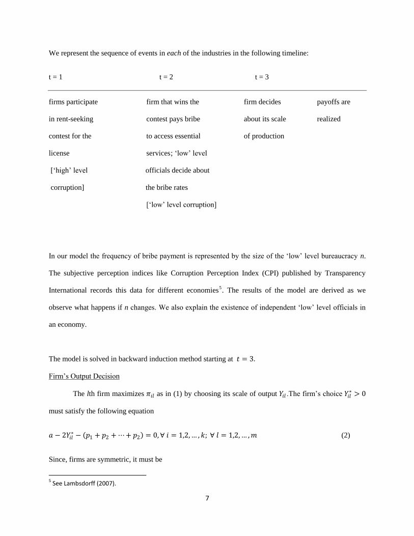
We represent the sequence of events in each of the industries in the following timeline:

t = 1 t = 2 t = 3

firms participate firm that wins the firm decides payoffs are

in rent-seeking contest pays bribe about its scale realized

contest for the to access essential of production

license services ; „low‟ level

[„high‟ level officials decide about

corruption] the bribe rates

[„low‟ level corruption]

In our model the frequency of bribe payment is represented by the size of the „low‟ level bureaucracy n.

The subjective perception indices like Corruption Perception Index (CPI) published by Transparency

International records this data for different economies5. The results of the model are derived as we

observe what happens if n changes. We also explain the existence of independent „low‟ level officials in

an economy.

The model is solved in backward induction method starting at 𝑡 = 3.

Firm‟s Output Decision

The lth firm maximizes 𝜋𝑖𝑙 as in (1) by choosing its scale of output 𝑌𝑖𝑙 .The firm‟s choice 𝑌𝑖𝑙∗ > 0

must satisfy the following equation

𝑎 − 2𝑌𝑖𝑙∗ − 𝑝1 + 𝑝2 + ⋯+ 𝑝2 = 0,∀ 𝑖 = 1,2,… ,𝑘; ∀ 𝑙 = 1,2,… ,𝑚 (2)

Since, firms are symmetric, it must be

5 See Lambsdorff (2007).

8

𝑌𝑖𝑙∗ = 𝑌∗,∀ 𝑖 = 1,2,… ,𝑘; ∀ 𝑙 = 1,2,… ,𝑚

Therefore, each firm‟s choice is given by:

𝑌∗ =1

2[𝑎 − 𝑝1 + 𝑝2 + ⋯+ 𝑝𝑛 ] (3)

„Low‟ Level Corruption

We assume the corruption that exists at the „low‟ level is without theft. Each official pays to the

government its per unit due 𝑐𝑗 for the provision of the input6. Since each of the k firms that have won the

rent-seeking competition at 𝑡 = 1 demand one unit of input from each of the n number of heterogeneous

government officials, the amount of input demanded from the jth official is given by 𝑥𝑗 = 𝑘𝑌∗,∀ 𝑗 =

1,2,… ,𝑛. Therefore the payoff function of the jth official is:

∅𝑗 = 𝑝𝑗 − 𝑐𝑗 𝑘𝑌∗, ∀ 𝑗 = 1,2,… ,𝑛 (4)

where, ∅𝑗 : payoff of the jth official.

Substituting 𝑌∗ from equation (3) in equation (4) the payoff of the jth official can be written as:

∅𝑗 𝑝1 ,… ,𝑝𝑛 =𝑘

2 𝑝𝑗 − 𝑐𝑗 𝑎 − 𝑝𝑗 − 𝑝1 + ⋯+ 𝑝𝑗−1 + 𝑝𝑗+1 + ⋯+ 𝑝𝑛 ,∀ 𝑗 = 1,2,… ,𝑛 (5)

Each official maximizes his own profit by choosing 𝑝𝑗∗. Assuming that an interior solution exists, 𝑝𝑗

∗ must

satisfy the following equation

𝑎 − 𝑝𝑗∗ − 𝑝ℎ𝑗≠ℎ − 𝑝𝑗

∗ − 𝑐𝑗 = 0, ∀ 𝑗 = 1,2,… ,𝑛 (6)

The system of equation (6) represents the reaction function of the jth official with respect to the price

charged by all other officials. The Nash equilibrium prices (𝑝1∗,… ,𝑝𝑗

∗,… ,𝑝𝑛∗) must satisfy the n equations

6 See Shleifer and Vishny (1993) for the definition of ‘corruption without theft’ and ‘corruption with theft’. In the

case of ‘corruption with theft’ essentially we have 𝑐𝑗 = 0. However, all the results of the present paper go through

for the case 𝑐𝑗 = 0.

9

given in (6). Defining 𝑃∗ = 𝑝𝑗∗𝑛

𝑗=1 , we can calculate 𝑃∗ by summing up the n equations given in (6) to

obtain:

𝑃∗ =𝑛𝑎 + 𝑐𝑗

𝑛𝑗=1

𝑛+1

Substituting the value of 𝑃∗ in equation (3) we obtain

𝑌∗ =𝑎− 𝑐𝑗

𝑛𝑗=1

2(𝑛+1)

Assumption 1: 𝑐 𝑛 = 𝑐𝑗𝑛𝑗=1 , 𝑐′(𝑛) ≥ 0.

The government may reduce the number of „low level‟ officials either by discontinuing some of the

services it provides or by clubbing them under less number of officials. In the first case, since the services

are essential, the firms cannot do away with them and must purchase them from the market. We assume

the market for these services are competitively supplied and consequently the total cost payable by a firm

for these services either remains the same or falls. In the second case, even if the number of officials falls,

since the services are clubbed under the new department, the cost of each of the redefined service

increases. Therefore, we assume the total cost payable by a firm either remains the same or falls.

Following assumption 1, the values of 𝑃∗ and 𝑌∗ can be written as:

𝑃∗ =𝑛𝑎 +𝑐(𝑛)

𝑛+1 (7)

𝑌∗ =𝑎−𝑐(𝑛)

2(𝑛+1) (8)

Assumption 2: 𝑎 > 𝑐(𝑛)

Assumption 2 ensures that 𝑌∗ > 0. Otherwise, 𝑌∗ = 0.

The total amount of bribe collected by all the n number of „low‟ level officials is:

10

𝐵∗ = ∅𝑗∗𝑛

𝑗=1 = 𝑘𝑌∗ (𝑝𝑗∗𝑛

𝑗=1 − 𝑐𝑗 ).

By summing over all n officials from equation (4) and substituting the values of 𝑃∗ and 𝑌∗ we get

𝐵∗ =1

2𝑘𝑛

𝑎 − 𝑐(𝑛)

𝑛 + 1

2

Using the expression of 𝑌∗ from (8) 𝐵∗ can be written as:

𝐵∗ = 2𝑘𝑛(𝑌∗)2 (9)

„High‟ Level Corruption

Substituting the values of 𝑃∗ and 𝑌∗ into (1), expected payoff level of the firm that wins the

competition for entering the industry is calculated as

𝜋𝑖𝑙∗ = 𝑧𝑖𝑙(𝑌

∗)2 − 𝑅𝑖𝑙 ,∀ 𝑖 = 1,2,… ,𝑘; 𝑙 = 1,2,… ,𝑚 (10)

Since each firm pays 𝑅𝑖𝑙 as bribe to the high-level official; the „contest success function‟ suggests that it

must be

𝑧𝑖𝑙 = 𝑅𝑖𝑙 𝑅𝑖𝑙 + (𝑅𝑖1 + ⋯+ 𝑅𝑖𝑙−1 + 𝑅𝑖𝑙+2 + ⋯+ 𝑅𝑖𝑚 ) −1,∀ 𝑖 = 1,2,…𝑘; 𝑙 = 1,2,… ,𝑚

So each firm ends up maximizing

𝜋𝑖𝑙∗ = 𝑅𝑖𝑙 𝑅𝑖𝑙 + (𝑅𝑖1 + ⋯+ 𝑅1𝑙−1 + ⋯+ 𝑅𝑖𝑙+1 + ⋯+ 𝑅𝑖𝑚 ) −1(𝑌∗)2 − 𝑅𝑖𝑙 ,

∀ 𝑖 = 1,2,… ,𝑘; 𝑙 = 1,2,… ,𝑚

by choosing an appropriate value of 𝑅𝑖𝑙∗ .

Since the participating firms in the rent-seeking game are symmetric it must be 𝑅𝑖𝑙∗ = 𝑅𝑖

∗,∀ 𝑙 =

1,2,… ,𝑚; 𝑖 = 1,2,…𝑘. The symmetric Nash equilibrium must satisfy the following equation:

[𝑅𝑖∗ + 𝑚 − 1 𝑅𝑖

∗]−1 𝑌∗ 2 − 𝑅𝑖∗[𝑅𝑖

∗ + 𝑚 − 1 𝑅𝑖∗]−2 𝑌∗ 2 = 1,∀ 𝑖 = 1,2,… ,𝑘

11

This solves for

𝑅𝑖∗ =

𝑚− 1

𝑚2 𝑌∗ 2 ,∀ 𝑖 = 1,2,… ,𝑘

Hence, the total amount of „high‟ level bribe given by all the m firms in the ith industry will be

𝑅𝑖∗ = 𝑚𝑅𝑖

∗ =𝑚−1

𝑚 𝑌∗ 2 (11)

Since all the industries are identical,

𝑅𝑖∗ = 𝑅∗,∀ 𝑖 = 1,2,… , 𝑘

And hence, the size of „high‟ level corruption in the economy is:

𝐻∗ = 𝑘𝑅∗ = 𝑘𝑚−1

𝑚(𝑌∗)2 (12)

Definition 1. The overall level of corruption (𝑇∗) in an economy is the sum of the amounts of bribe paid

by all the firms both at the „high‟ as well as the „low‟ levels in all the industries that belong to the

economy, i.e.

𝑇∗ = 𝐻∗ + 𝐵∗. (13)

Definition 2. The welfare of the economy is defined as:

𝑊 = 𝑤 𝑘𝑌∗ where 𝑤 ′ > 0.

Note that since the bribe payments are transfers from firms to the officials within the economy they do not

enter the welfare calculation. Also note that definition 2 deals only with the static efficiency of the

economy. But the distribution of rent from the firms which are productive agents to the bureaucrats who

are unproductive agents creates dynamic inefficiency for the economy, too.

12

In the next section we use this model to find out the effect of rise in size of „low‟ level

bureaucracy (equivalent to frequency of bribe payment) on the size of the „high‟ level corruption in an

economy. We also derive the effect of the same on the size of overall corruption and the welfare of the

economy. Then we explore the condition under which a coalition between the „high‟ and „low‟ level

officials forms. We compare the overall corruption level of an economy where such a coalition forms

against the overall corruption of an economy where such a coalition does not form.

3. Results

Observation 1: 𝑑𝑌∗

𝑑𝑛< 0.

Proof: From (8)

𝑑𝑌∗

𝑑𝑛= −

1

2(𝑛+1)2 [𝑎 − 𝑐 𝑛 + 𝑛 + 1 𝑐′ 𝑛 ] (14)

The statement of the observation follows from application of assumptions 1 and 2 of the model. □

Note from (7), 𝑑𝑃∗

𝑑𝑛=

𝑎−𝑐 𝑛 + 𝑛+1 𝑐 ′ (𝑛)

(𝑛+1)2 . By assumptions 1 and 2, 𝑑𝑃∗

𝑑𝑛> 0. So as the number of „low‟

level officials increases, the marginal cost of production 𝑃∗ for each of the firm increases. Hence, output

of each of them falls, causing a fall in the aggregate output. The opposite happens when the number of

„low‟ level officials falls. The aggregate output expands.

Proposition 1: As the frequency of bribery increases (decreases), the size of ‘high’ level corruption falls

(rises).

Proof: The frequency of bribery increases as n increases. From (12) we get:

𝑑𝐻∗

𝑑𝑛= 2𝑘𝑌∗ 𝑚−1

𝑚

𝑑𝑌∗

𝑑𝑛

13

Since 𝑚 ≥ 2, with the help of observation 1we observe:

𝑑𝐻∗

𝑑𝑛< 0 (15)

Therefore, the statement of proposition follows. □

As the number of „low‟ level officials increases, marginal cost of each firm increases. Consequently, their

operating profit falls. This reduces the obtainable rent from the k th industry. So the total amount of bribe

paid by firms in competing to enter k th industry falls. As all the industries are identical, the total amount

paid at the „high‟ level falls.

Proposition 2: As the frequency of bribery increases (decreases), the size of overall corruption of an

economy falls (rises); the welfare of the economy also falls (rises).

Proof: The frequency of bribery increases as n increases. From Definition 1, it follows:

𝑑𝑇∗

𝑑𝑛=

𝑑𝐻∗

𝑑𝑛+

𝑑𝐵∗

𝑑𝑛. (16)

From (15) we know: 𝑑𝐻∗

𝑑𝑛 < 0. From (9) we derive:

𝑑𝐵∗

𝑑𝑛= 2𝑘(𝑌∗)2 + 4𝑘𝑛𝑌∗

𝑑𝑌∗

𝑑𝑛

By substituting from equations (8) and (14) in the expression of 𝑑𝐵∗

𝑑𝑛 we obtain:

𝑑𝐵∗

𝑑𝑛= −

𝑘𝑌∗

𝑛 + 1 2 𝑛 − 1 𝑎 − 𝑐 𝑛 + 2𝑛 𝑛 + 1 𝑐′ 𝑛

Given assumptions 1and 2, and the fact that 𝑛 ≥ 2, 𝑑𝐵∗

𝑑𝑛< 0. Hence from (16) the statement of the first

part of the proposition follows.

14

For the second part of the proposition we use Definition 2. Since 𝑑𝑌∗

𝑑𝑛< 0, clearly

𝑑𝑊

𝑑𝑛= 𝑤 ′ 𝑘

𝑑𝑌∗

𝑑𝑛 < 0. □

In a recent paper, which exclusively deals with „low‟ level corruption, Zenger (2011) has shown that

𝑑𝐵∗

𝑑𝑛< 0 and

𝑑𝑊

𝑑𝑛 < 0. Our paper shows that similar result holds even if we consider the scope of „high‟

level corruption in an economy. It turns out that the higher frequency of „low‟ level bribes acts as a check

on the overall level of corruption in an economy. The size of „low‟ level corruption itself falls as the

demand for the „low‟ level officials‟ services falls as the firms scale down their operation. As the

expected operating profit of the firms falls, demand for licenses of these industries falls as well.

Consequently, the high level corruption falls. But as the total output of the economy falls, the welfare

level of the economy also falls. So proposition 2 points out that in economies where we observe

independent „low‟ level bureaucrats the overall size of corruption and its welfare level can go hand in

hand.

Proposition 2 also explains the way the CPI ranking is based on the data on „frequency‟ of

bribery in different economies may be misleading in comparison of overall corruption level of the

economies. The economies with higher frequency of bribery must be having lower overall level of

corruption.

One natural question that arises from the above results is that since the presence of „low‟ level

officials reduces the bribe revenue of the high level officials in each of the industries, why not these

officials try to strike out a coalition with the „low‟ level officials. Such a coalition by eliminating the

double marginalization effect that each one of the „low‟ level officials imposes on the other would have

reduced the marginal cost of production of the firms. The higher output produced by the firms could

increase payoff of the high level officials. Would the „low‟ level officials agree to participate in such a

coalition? Note that from participating in such a coalition the „low‟ level officials would lose the bribe-

rent they were enjoying without the coalition. Therefore such a coalition would form if the high level

15

officials with their higher payoff could compensate the loss of the „low‟ level officials from participating

in it. The analysis below explains the possibility of coalition formation in details.

The coalition between the „high‟ level official in the ith industry and the „low‟ level officials

would form if all the „low‟ level officials agree to charge the respective official prices for the services

they provide to the firm which wins the license to operate in ith industry and thus avoids the double

marginalization. So in case of coalition between „high‟ and „low‟ level officials the jth „low‟ level official

(∀ 𝑗 = 1,2,… ,𝑛) charges:

𝑝𝑗 = 𝑐𝑗 .

Now, the profit of the l th firm that wins the license to operate in the ith industry can be written as:

𝜋𝑖𝑙 = 𝑧𝑖𝑙 𝑎 − 𝑌𝑖𝑙 𝑌𝑖𝑙 − 𝑐1 + 𝑐2 + ⋯+ 𝑐𝑛 𝑌𝑖𝑙 − 𝑅𝑖𝑙 (17)

The profit maximizing choice of output level 𝑌𝑖𝑙′ > 0 must satisfy the following equation:

𝑎 − 2𝑌𝑖𝑙′ − 𝑐1 + 𝑐2 + ⋯+ 𝑐𝑛 = 0

Since due to symmetry 𝑌𝑖𝑙′ = 𝑌′ ,∀ 𝑖 = 1,2,… ,𝑘; ∀ 𝑙 = 1,2,… ,𝑚.

𝑌′ =1

2 𝑎 − 𝑐𝑗

𝑛𝑗=1 .

From assumption 1 the value of 𝑌′ can be rewritten as

𝑌′ =1

2[𝑎 − 𝑐 𝑛 ] (18)

Using (18), from (17) the expected payoff of the lth firm that participates in the contest to take entry in

the ith industry can be written as:

𝜋𝑖𝑙′ = 𝑧𝑖𝑙 𝑌

′ 2 − 𝑅𝑖𝑙 ,∀ 𝑖 = 1,2,… ,𝑘;∀ 𝑙 = 1,2,… ,𝑚

16

where 𝑅𝑖𝑙 is the bribe to the „high‟ level official responsible for awarding license in the ith industry and

𝑧𝑖𝑙 is the „contest success function‟. Substituting the value of 𝑧𝑖𝑙 in the expression of 𝜋𝑖𝑙′ we obtain:

𝜋𝑖𝑙′ = 𝑅𝑖𝑙 𝑅𝑖𝑙 + 𝑅𝑖1 + ⋯+ 𝑅𝑖𝑙−1 + 𝑅𝑖𝑙+1 + ⋯+ 𝑅𝑖𝑚 −1 𝑌′ 2 − 𝑅𝑖𝑙 ,∀ 𝑖 = 1,2,… ,𝑘;

∀ 𝑙 = 1,2,… ,𝑚.

Suppose 𝑅𝑖𝑙′ maximizes 𝜋𝑖𝑙

′ 𝑓𝑜𝑟 ∀ 𝑖 = 1,2,… ,𝑘;∀ 𝑙 = 1,2,…𝑚. By symmetry of the firms it must be

𝑅𝑖𝑙′ = 𝑅𝑖

′ where 𝑅𝑖′ satisfies the following equation

[𝑅𝑖′ + 𝑚 − 1 𝑅𝑖

′ ]−1 𝑌′ 2 − 𝑅𝑖′ [𝑅𝑖

′ + 𝑚 − 1 𝑅𝑖′ ]−2 𝑌′ 2 = 1,∀ 𝑖 = 1,2,… ,𝑘

This solves for 𝑅𝑖′ =

𝑚−1

𝑚2 𝑌′ 2.

Hence, the total amount of bribe accrued to the „high‟ level official at the ith industry becomes

𝑅 𝑖′ =

𝑚−1

𝑚 𝑌′ 2 (19)

Out of 𝑅 𝑖′ the „high‟ level official at the ith industry pays out (𝑝𝑗

∗ − 𝑐𝑗 )𝑌∗ to the jth „low‟ level official

(∀ 𝑗 = 1,2,… ,𝑛) to compensate for her loss from participating in the coalition. The total compensation

paid to all the n „low‟ level officials turns out to be [𝑌∗ (𝑝𝑗∗𝑛

𝑗=1 − 𝑐𝑗 )]. The coalition is feasible if 𝑅 𝑖′ -

𝑌∗ (𝑝𝑗∗𝑛

𝑗=1 − 𝑐𝑗 ) ≥ 𝑅𝑖∗ .

However, the feasibility of the coalition does not ensure its stability. The „high‟ level official at

the ith industry observes that the terms and conditions of the coalition described above do not prevent

unilateral deviation by any one of the n „low‟ level officials from the agreed terms of the coalition. The jth

official can profitably deviate from charging the official price 𝑐𝑗 for the jth service by charging 𝑝𝑗′ > 𝑐𝑗 on

the assumption that all other officials will not deviate and will continue to charge the official price for

their services. The jth low level official chooses 𝑝𝑗′ to maximize her deviation payoff [ 𝑝𝑗

′ − 𝑐𝑗 𝑌" +

17

( 𝑝𝑗∗ − 𝑐𝑗 )𝑌∗ ] where 𝑌" =

1

2[𝑎 − (𝑐1 + ⋯+ 𝑐𝑗−1 + 𝑝𝑗

′ + 𝑐𝑗+1 + ⋯+ 𝑐𝑛)] . Since [ 𝑝𝑗′ − 𝑐𝑗 𝑌

" + ( 𝑝𝑗∗ −

𝑐𝑗 )𝑌∗] > (𝑝𝑗∗ − 𝑐𝑗 )𝑌∗ the deviation always takes place ∀ 𝑗 = 1,2,… ,𝑛 and the coalition breaks down.

It is possible to show that the deviation from the coalition is prevented through payment of an

incentive 𝑡′ = (𝑎 − 𝑐 𝑛 )𝑌" to the jth official. With such an incentive scheme the jth official chooses 𝑝𝑗′

by maximizing [ 𝑝𝑗′ − 𝑐𝑗 + (𝑎 − 𝑐 𝑛 ) 𝑌"]. The first order condition for maximization solves for 𝑝𝑗

′ = 𝑐𝑗 .

Therefore the deviation is prevented for all 𝑗 = 1,2,… ,𝑛 and 𝑌" = 𝑌′ . If (𝑎 − 𝑐 𝑛 )𝑌′ ≥ (𝑝𝑗∗ − 𝑐𝑗 )𝑌∗,

just by paying (𝑎 − 𝑐 𝑛 )𝑌′ to each of the officials the „high‟ level official can ensure both participation

in the coalition, as well as non-deviation from it. The total payment to the „low‟ level officials in this case

is: 𝑛(𝑎 − 𝑐 𝑛 )𝑌′ . Otherwise, she has to pay (𝑝𝑗∗ − 𝑐𝑗 )𝑌∗ to the jth „low‟ level official and 𝑌∗ (𝑝𝑗

∗𝑛𝑗=1 −

𝑐𝑗 ) = 𝑌∗(𝑃∗ − 𝑐(𝑛)) to all of them. By substituting the values of 𝑌∗, 𝑃∗, 𝑌′ from (8), (7) and (18) in the

respective expressions we observe, 𝑛(𝑎 − 𝑐 𝑛 )𝑌′ > 𝑌∗(𝑃∗ − 𝑐(𝑛)). So the sufficient condition for

existence of a stable coalition turns out to be

𝑅 𝑖′ - 𝑛(𝑎 − 𝑐 𝑛 )𝑌′ ≥ 𝑅𝑖

∗ . ∀ 𝑖 = 1,2,… ,𝑘 (20)

Proposition 3: A stable coalition between the ‘high’ and the independent ‘low’ level officials never

forms.

Proof: A stable coalition between the „high‟ and the independent „low‟ level officials successfully forms

if condition (20) holds.

Substituting the values of 𝑅 𝑖′ , 𝑌′ and 𝑅𝑖

∗ respectively from (19), (18) and (11) in (20) we conclude that

inequality (20) holds if the following inequality holds:

𝑚[1 −2𝑛(𝑛+1)2

𝑛+1 2−1] ≥ 1.

18

But since 2𝑛(𝑛+1)2

𝑛+1 2−1 > 1 for all values of 𝑛 ≥ 2 and 𝑚 ≥ 2, the above inequality never holds. Therefore

inequality (20) can never hold in reality. The statement of the proposition follows. □

Proposition 3 explains why we observe corrupt independent „low‟ level officials in an economy. Although

official-price-charging-„honest‟ „low‟ level officials are desirable for the interest of the „high‟ level

officials and from the welfare perspective of the economy as well, the „low‟ level corruption persists.

Thus the proposition provides an explanation behind the empirical observation made by De Soto (2000)

that in many developing countries, quite contrary to the expectation, large number of independent „low‟

level officials exists. The existence of „large‟ number of independent complementary-service-providing

officials on the other hand explains low income level of these countries.

3. Conclusions

This paper explores the relation between frequency of bribery and the level of corruption in an

economy. It presents a model of bureaucracy in an economy with independent „high‟ and „low‟ level

bureaucrats, both the levels being corruptible. The „high‟ level corruption points out to the high level

bureaucrats who take advantage of their position of power and provide preferential treatment to the firms

against rent-seeking activity or gainful lobbying. On the other hand the situation of low level bureaucrats

selling essential services to firms in exchange of bribe consists of „low‟ level corruption. The number of

„low‟ level bureaucrats proxies for „frequency‟ of bribe demand a representative firm faces conducting its

operation in these economies. The model exploits the conjecture expressed in Lambsdorff (2007) that the

increase in power of the corruptible bureaucrats works as an inherent check on the level of corruption in

the economies in deriving its main results. Here the increase in bribe frequency reduces the scale of

operation of the firms by increasing their marginal cost of production and thereby adversely affects the

bribe revenue collected both at „high‟ and „low‟ levels of bureaucracy. The overall corruption of the

economy also falls.

19

The paper contributes to the literature in three important ways: first, it argues that the ranking of

the economies as reported by Corruption Perception Index (CPI) published by the organizations like

Transparency International based on bribe “frequency” data may not reflect the ranking of the economies

according to their overall size of corruption; second, it points out that higher bribe “frequency” in an

economy as reflected in CPI is indicator of lower size of „high‟ level corruption in the economy; third, it

explains why a stable coalition between the „high‟ and „low‟ level bureaucrats does not materialize and

therefore it explains why we observe high „low‟ level bribe frequency as we observe it in the low income

countries. The paper also provides a new explanation of why we do not observe „kleptocracies‟ in most

of the real world situations.

The results derived in the paper imply that the well known policy rhetoric like controlling bribe

„frequency‟ or controlling power of „low‟ level bureaucrats may indeed bring about economic

development but may fail to control the overall size of corruption in economies. Therefore policies for

controlling the overall size of corruption and the policies for promoting economic development must be

different from each other. The high overall size of corruption can be seen as the price paid for high level

of economic development.

How important are the assumptions made in the model? The assumption of symmetry of the

industries present in the economy helps to simplify calculations of the model. However the results are not

dependent on this assumption. In industries with inelastic demand pattern although the effect of increased

bribe „frequency‟ would be limited, since it would be very pronounced in the industries with elastic

demand, in aggregate the results of the model would still go through. Similarly if less number of firms

compete for entry in an industry, the „high‟ level bribe revenue falls in that particular industry; but this

keeps the results unchanged. The model also assumes that corruption does not lead to exit of firms from

the industry. This assumption is also not crucial for validity of the results of the model. In fact Zenger

(2011) taking into account the possibility of exit in his model derives similar result as Proposition 2 of our

model in the case of „low‟ level corruption in economies. In the model we do not take into account of

20

punishment on the corrupt bureaucrats. The assumption is supported by the fact that in economies with

independent bureaucrats, the bureaucrats derive their independence from lack of effective punishment

from the higher authority. But even if we introduce punishment for the „low‟ level bureaucrats in our

model, as long as it fails to eliminate „low‟ level corruption, it merely increases the marginal cost of the

essential inputs they supply to the firms, and therefore does not have any effect on the results derived in

the paper.

The model can have many interesting applications. It can be used to study the effect of bribe

frequency on the concentration and size distribution of firms in an industry. It can also be used to study

the effect of trade liberalization in an economy. In particular it can be used to throw light on the necessity

of bureaucratic reform along with the trade liberalization. These remain as our future research agenda.

21

References

Bliss, C. and R. Di Tella (1997): Does Competition Kill Corruption? Journal of Political Economy, 105

(5), 1001-1023.

Celentani, M., J. J. Ganuza and J. L. Peydro (2004): Combating Corruption in International Business

Transactions, Economica 71, 417 – 448.

De Soto, H (2000): The Mystery of Capitalism, Basic Books: New York.

Grossman, S. J. (1995): Dynamic Asset Allocation and the Informational Efficiency of Markets, Journal

of Finance L (3) , 773-787.

Kahana, N. and S. Nitzan (2002): Pre-assigned Rents and Bureaucratic Friction, Economics of

Governance 3, 241 – 248.

Lambsdorff, J.G. (2001): How Corruption in Government Affects Public Welfare – A Review of

Theories, Centre for Globalization and Europeanization of the Economy, Gottingen, Discussion Paper 9.

Lambsdorff, J.G. (2007): The Institutional Economics of Corruption & Reform-Theory, Evidence and

Policy, Cambridge University Press: Cambridge.

Moe, T. M. (1984): The New Economics of Organization, American Journal of Political Science 28 (4),

739-777.

Mookherjee, D. and I.P.L. Png (1995): Corruptible law Enforcers: How Should They Be Compensated,

The Economic Journal 105 (428),145-159.

Olken, B.A. and P. Barron (2009): The Simple Economics of Extortion: Evidence from Trucking in

Aceh, Journal of Political Economy 3 (117), 417-452.

Shleifer, A. and R. Vishny (1993): Corruption, Quarterly Journal of Economics 108 (3), 599-617.

22

Zenger, H. (2011): Uncoordinated Corruption as an Equilibrium Phenomenon, Journal of Institutional

and Theoretical Economics 167, 343-351.