Vladica Andrejic

GEOMETRY

(26-05-2018)

The History of every major Galactic Civilization tends to pass through three distinct and recognizablephases, those of Survival, Inquiry and Sophistication, otherwise known as the How, Why, and Wherephases. For instance, the rst phase is characterized by the question "How can we eat?" the second bythe question "Why do we eat?" and the third by the question "Where shall we have lunch?"

Douglas AdamsThe Hitchhikers Guide to the Galaxy

i

Contents

1 Smooth manifolds 11.1 Historical introduction . . . . . . . . . . . . . . . . . . . . . . . . . . . . . . . . . . . . . . 11.2 Topological manifolds . . . . . . . . . . . . . . . . . . . . . . . . . . . . . . . . . . . . . . 21.3 Topological properties of manifolds . . . . . . . . . . . . . . . . . . . . . . . . . . . . . . . 51.4 Smooth manifolds . . . . . . . . . . . . . . . . . . . . . . . . . . . . . . . . . . . . . . . . 71.5 Quotient manifolds . . . . . . . . . . . . . . . . . . . . . . . . . . . . . . . . . . . . . . . . 101.6 Smooth maps . . . . . . . . . . . . . . . . . . . . . . . . . . . . . . . . . . . . . . . . . . . 111.7 Partitions of unity . . . . . . . . . . . . . . . . . . . . . . . . . . . . . . . . . . . . . . . . 151.8 Tangent vectors . . . . . . . . . . . . . . . . . . . . . . . . . . . . . . . . . . . . . . . . . . 181.9 Tangent maps . . . . . . . . . . . . . . . . . . . . . . . . . . . . . . . . . . . . . . . . . . . 211.10 Submersions and immersions . . . . . . . . . . . . . . . . . . . . . . . . . . . . . . . . . . 231.11 Submanifolds . . . . . . . . . . . . . . . . . . . . . . . . . . . . . . . . . . . . . . . . . . . 251.12 Vector elds . . . . . . . . . . . . . . . . . . . . . . . . . . . . . . . . . . . . . . . . . . . . 261.13 Global tangent maps . . . . . . . . . . . . . . . . . . . . . . . . . . . . . . . . . . . . . . . 291.14 Local and global frames . . . . . . . . . . . . . . . . . . . . . . . . . . . . . . . . . . . . . 311.15 Covector elds . . . . . . . . . . . . . . . . . . . . . . . . . . . . . . . . . . . . . . . . . . 331.16 Tensor elds . . . . . . . . . . . . . . . . . . . . . . . . . . . . . . . . . . . . . . . . . . . . 351.17 Tensor derivations . . . . . . . . . . . . . . . . . . . . . . . . . . . . . . . . . . . . . . . . 38

2 Pseudo-Riemannian geometry 412.1 Scalar products . . . . . . . . . . . . . . . . . . . . . . . . . . . . . . . . . . . . . . . . . . 412.2 Isotropic vectors and spaces . . . . . . . . . . . . . . . . . . . . . . . . . . . . . . . . . . . 432.3 Metrics . . . . . . . . . . . . . . . . . . . . . . . . . . . . . . . . . . . . . . . . . . . . . . 452.4 Musical isomorphisms . . . . . . . . . . . . . . . . . . . . . . . . . . . . . . . . . . . . . . 482.5 Covariant derivatives . . . . . . . . . . . . . . . . . . . . . . . . . . . . . . . . . . . . . . . 482.6 Christoel symbols . . . . . . . . . . . . . . . . . . . . . . . . . . . . . . . . . . . . . . . . 502.7 Levi-Civita connection . . . . . . . . . . . . . . . . . . . . . . . . . . . . . . . . . . . . . . 512.8 Parallel transport . . . . . . . . . . . . . . . . . . . . . . . . . . . . . . . . . . . . . . . . . 532.9 Geodesics . . . . . . . . . . . . . . . . . . . . . . . . . . . . . . . . . . . . . . . . . . . . . 562.10 Exponential map . . . . . . . . . . . . . . . . . . . . . . . . . . . . . . . . . . . . . . . . . 582.11 Curvature tensor elds . . . . . . . . . . . . . . . . . . . . . . . . . . . . . . . . . . . . . . 592.12 Algebraic curvature tensors . . . . . . . . . . . . . . . . . . . . . . . . . . . . . . . . . . . 632.13 Sectional curvature . . . . . . . . . . . . . . . . . . . . . . . . . . . . . . . . . . . . . . . . 652.14 Constant sectional curvature . . . . . . . . . . . . . . . . . . . . . . . . . . . . . . . . . . 662.15 Ricci curvature . . . . . . . . . . . . . . . . . . . . . . . . . . . . . . . . . . . . . . . . . . 69

3 Osserman manifolds 723.1 Eigen-structure of linear operators . . . . . . . . . . . . . . . . . . . . . . . . . . . . . . . 723.2 Osserman conditions . . . . . . . . . . . . . . . . . . . . . . . . . . . . . . . . . . . . . . . 743.3 Osserman algebraic curvature tensor . . . . . . . . . . . . . . . . . . . . . . . . . . . . . . 783.4 Einstein, zwei-stein . . . . . . . . . . . . . . . . . . . . . . . . . . . . . . . . . . . . . . . . 803.5 Lorentzian Osserman . . . . . . . . . . . . . . . . . . . . . . . . . . . . . . . . . . . . . . . 823.6 Schur problems . . . . . . . . . . . . . . . . . . . . . . . . . . . . . . . . . . . . . . . . . . 833.7 Any-stein . . . . . . . . . . . . . . . . . . . . . . . . . . . . . . . . . . . . . . . . . . . . . 86

ii

3.8 Duality principle . . . . . . . . . . . . . . . . . . . . . . . . . . . . . . . . . . . . . . . . . 893.9 Quasi-Cliord curvature tensors . . . . . . . . . . . . . . . . . . . . . . . . . . . . . . . . . 913.10 Quasi-Cliord duality . . . . . . . . . . . . . . . . . . . . . . . . . . . . . . . . . . . . . . 923.11 Cliord total duality . . . . . . . . . . . . . . . . . . . . . . . . . . . . . . . . . . . . . . . 943.12 Anti-Cliord curvature tensor . . . . . . . . . . . . . . . . . . . . . . . . . . . . . . . . . . 953.13 Four-dimensional Osserman . . . . . . . . . . . . . . . . . . . . . . . . . . . . . . . . . . . 963.14 Converse problem . . . . . . . . . . . . . . . . . . . . . . . . . . . . . . . . . . . . . . . . . 993.15 Four-dimensional Jacobi-dual . . . . . . . . . . . . . . . . . . . . . . . . . . . . . . . . . . 1003.16 Lorentzian Jacobi-dual . . . . . . . . . . . . . . . . . . . . . . . . . . . . . . . . . . . . . . 1023.17 Fiedler tensors . . . . . . . . . . . . . . . . . . . . . . . . . . . . . . . . . . . . . . . . . . 1033.18 Two-leaves Osserman . . . . . . . . . . . . . . . . . . . . . . . . . . . . . . . . . . . . . . . 1043.19 Quasi-special Osserman . . . . . . . . . . . . . . . . . . . . . . . . . . . . . . . . . . . . . 107

Bibliography 111

iii

Chapter 1

Smooth manifolds

The rst chapter is an introduction to smooth manifolds. We introduce the basic mathematical objects,notation and terminology which will be used throughout this book. The material of this chapter borrowsfrom many sources, including the standard texts on manifolds and dierential geometry: O'Neill1 [59],Lee2 [46], Lee3 [47], Gallier4 [37], Morita5 [52], Tu6 [67]. For a topological side of view we recommendCrainic7 [22].

1.1 Historical introduction

One of the most signicant events in the history of geometry was on June 10, 1854, when BernhardRiemann8 held a public lecture entitled ½On the hypotheses which lie at the foundations of geometry( Uber die Hypothesen, welche der Geometrie zu Grunde liegen) at the Philosophical Faculty at Gottingen.

In 1851, Riemann completed his doctoral dissertation (it was on the foundations of complex analysis)under Gauss's9 supervision. The next step in his academic career was to qualify as a privatdocent, alecturer who received no salary, but was merely forwarded fees paid by these students who elected toattend his lectures.

This position was obtained through the process of habilitation, where candidates were asked to submitan inaugural paper (habilitationsschrift) as well as to hold a public lecture (habilitationsvortrag). Aninaugural lecture topic was chosen by the faculty from a list of three proposals made by the candidate.The rst two topics which Riemann submitted were ones on which he had already worked. However,Riemann was taken by surprise when Gauss, contrary to tradition, passed over the rst two and pickedthe third, about the foundations of geometry.

Riemann worked hard to make the lecture understandable to non-mathematicians in the audience(there were only a few geometricians), so he had a great presentation in which the ideas were clearlydened without the help of analytic techniques. Although Gauss was very impressed since the lecturesurpassed all his expectations, the material was presented orally and without technical details, so it is notsurprising that the lecture did not achieve the immediate impact on the mathematical world. However,the rst publication of this lecture in 1868 (two years after Riemann's death) caused signicant reactionsof mathematicians and became a milestone in the history of geometry.

At that time was the investigation concerning Euclid's10 fth postulate, looking for axioms to solidlydene the basic space of geometry. There was also the quest of the structure of the space we are livingin, and some mathematicians were starting to think that other structures might exist. This led us to

1Barrett O'Neill (19242011), American mathematician2Jerey M Lee (1956), American mathematician3John M Lee (1950), American mathematician4Jean Henri Gallier (1949), French-American mathematician5Shigeyuki Morita (1946), Japanese mathematician6Loring Wuliang Tu (1952), Taiwanese-American mathematician7Marius Crainic (1974), Romanian-Dutch mathematician8Georg Friedrich Bernhard Riemann (18261866), German mathematician9Johann Carl Friedrich Gauß (17771855), German mathematician

10Euclid of Alexandria (. 300 BCE), Greek mathematican

1

the non-Euclidean geometries dealt with by Bolyai11 and Lobachevsky12 (and before them pioneeringworks had Saccheri13 and Omar Khayyam14), which suddenly become only special cases of more generaltheory.

Riemann was the rst to give a comprehensive contribution to the generalization of the idea of surfaceto more dimensions, and his vision gave a new concept of space for which he used the word manifold(mannigfaltigkeit). The famous Riemann's lecture and the story about it can be found at Spivak15 [64,Chapter 4].

Manifolds are the fundamental objects of Dierential Geometry. However, Riemann did not have aprecise denition of the concept. At that time it was technically impossible to give a formal denitionof topological spaces and to specify manifolds among them. Poincare16 in his 1895 work Analysus situsintroduced the idea of a manifold atlas and gave a denition of a manifold which served as a precursorto the modern concept of a manifold. The rst rigorous axiomatic denition of manifolds was given byVeblen17 and Whitehead18 only in 1931.

Manifolds are all around us in many guises and these can be seen as higher dimensional generalizationsof smooth curves and smooth surfaces. Generally speaking, these are geometrical objects that locallylook like some Euclidean space Rn, and on which one can do dierential and integral calculus. Of course,the basic examples of manifolds are Euclidean spaces themselves, smooth plane curves (such as ellipses,hyperbolas, and parabolas), and smooth surfaces (such as ellipsoids, hyperboloids, paraboloids, tori).Higher-dimensional examples include the unit n-sphere in Rn+1 and graphs of smooth maps betweenEuclidean spaces.

In contrast to mentioned examples, a manifold does not always appear in a well known space. Ingeneral it is rather dicult to think of it as a geometric gure, since it lives in a very abstract environment.However, when we nd local coordinates on such a set and study the relationship among them, it oftenhappens that a hidden geometric structure gradually comes to light. Since we want to involve as manyobjects as possible, it is unavoidable for the denition of manifolds to be abstract. Though, once anobject is recognized to be a manifold based on this abstract denition, it appears in a known spacethrough the coordinates, and turns out to be a very practical object.

1.2 Topological manifolds

The study of manifolds involves topology, so we assume that the reader is familiar with the denition andbasic properties of topological spaces. We can consider a topological space with certain properties thattell us what exactly means that it locally looks like an Euclidean space. However, this resemblance to anEuclidean space should be sharp enough to allow partial dierentiation and consequently all importantfeatures of dierential and integral calculus on a manifold. Once we have established the calculus ona manifold, many concrete applications are possible. We can compute a volume (by integration) ora curvature (by formulas involving second derivatives), we can work in classical mechanics (where wesolving systems of ordinary dierential equations) or general relativity (where we solving systems ofpartial dierential equations).

One can imagine a manifold as a dark room with a lamp available. At any given time, the lampwill permit us to look at a certain region of the room only, giving us a local idea about how the roomlooks like. The lamp here is an Euclidean space which comes equipped with a nice coordinate system.In studying the geography of the earth it is convenient to use geographical maps of various portions ofthe earth instead of examining the earth directly. A collection of geographical maps that cover the earthis called an atlas, and it gives an excellent description of what the earth is, without actually visualizingthe planet embedded in 3-space.

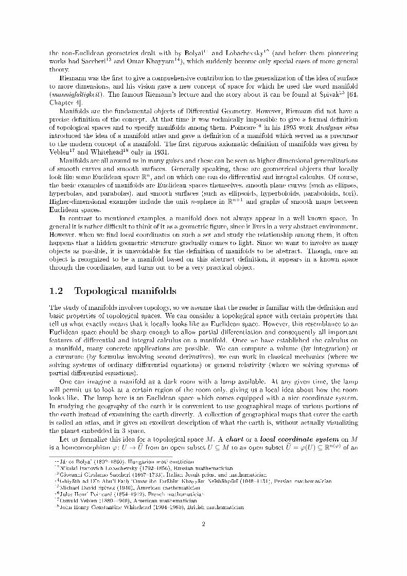
Let us formalize this idea for a topological space M . A chart or a local coordinate system on Mis a homeomorphism ϕ : U → U from an open subset U ⊆M to an open subset U = ϕ(U) ⊆ Rn(ϕ) of an

11Janos Bolyai (18021860), Hungarian mathematician12Nikolai Ivanovich Lobachevsky (17921856), Russian mathematician13Giovanni Girolamo Saccheri (16671733), Italian Jesuit priest and mathematician14Ghiyath ad-Dn Abu'l-Fath. Omar ibn Ibrahm Khayyam Neshahpur (10481131), Persian mathematician15Michael David Spivak (1940), American mathematician16Jules Henri Poincare (18541912), French mathematician17Oswald Veblen (18801960), American mathematician18John Henry Constantine Whitehead (19041960), British mathematician

2

Euclidean space. The domain U of a chart ϕ is called a coordinate neighbourhood , and because of thefrequent use, that chart ϕ can be traditionally recorded as the ordered pair (U,ϕ). We say that (U,ϕ)is a chart at p ∈ M if p ∈ U . An atlas on M is a collection of charts whose union of all coordinateneighbourhoods is M (every point of M is contained in the domain of some chart). We say that M islocally Euclidean of dimension n ∈ N0 if there is an atlas on M such that the codomain of eachchart is the Euclidean space Rn.

M

U

ϕ(U)

Rn

ϕ

A manifold requires that M is locally Euclidean of dimension n for some xed n ∈ N0. Usually,additional technical assumptions on the topological space are made to avoid some pathological examplesthat do not arise in practice. A common assumption is Hausdorness19, which means that for anytwo distinct points p, q ∈M there exist disjoint open subsets U, V ⊂M such that p ∈ U and q ∈ V . Anadditional requirement is that M is second countable (satisfying the second axiom of countability),which means that its topology has a countable basis. Although there are some important topologicalspaces that fail to satisfy our conditions, it can be said that almost all ordinary geometrical gures satisfythem.

For example, a Hausdor space has two essential properties. First, that the limit of a convergentsequence is unique. Second, that compact subsets are closed sets (especially, any nite set is closed)and thus have complements that are open. Hausdorness together with the second countability impliesthe existence of partitions of unity, a very important tool in a manifold theory, and would suce tojustify these conditions. It follows that these conditions ensure that every manifold embeds in somenite-dimensional Euclidean space, and it can be endowed with a Riemannian metric. A topologicalspace that fulls features of a topological structure mentioned above is called a topological manifold.

Denition 1.1. A topological n-manifold is a second countable Hausdor space which is locallyEuclidean of dimension n.

Example 1.1. The basic example of a topological n-manifold is, certainly, the Euclidean space Rn. Itis Hausdor because it is a metric space, and it is second countable because the set of all open ballswith rational centres and rational radii is a countable basis of the topology. It is locally Euclidean ofdimension n which can justify the single chart (Rn, IdRn). 4

Some authors decided to omit one of conditions from Denition 1.1, but it is extremely rare to meeta space in nature without all of these conditions. The properties in the topological manifold denitionare independent. Let us illustrate this with some esoteric examples.

Example 1.2. The line with two origins M = (x, y) : x ∈ R, y = ±1/∼ is the quotient space, wherethe equivalence relation ∼ is given by (x,−1) ∼ (x, 1), if x 6= 0. We can see it asM = (R\0)∪0A, 0Bwith a topology basis which contains all open intervals in R that do not contain 0, along with all setsof the form (−ε, 0) ∪ 0A ∪ (0, ε) and all sets of the form (−ε, 0) ∪ 0B ∪ (0, ε) for ε > 0. Of course,a countable basis consists of intervals having rational endpoints, along with rational ε. The obvioushomeomorphism f : M \ 0B → R is given by f(x) = x for x 6= 0A and f(0A) = 0. For example, taking0 < a < b, we have the preimage f−1(−a, b) = ((−a, 0)∪0A∪ (0, a))∪ (a/2, b), so f is continuous. Onecan also prove that f−1 is continuous. Since both M \ 0A and M \ 0B are homeomorphic to R, wesee that M is locally Euclidean of dimension 1. If M was a Hausdor space there would exist disjoint

19Felix Hausdor (18681942), German mathematician

3

open subsets containing 0A and 0B , so there would exist a, b > 0 such that (−a, 0) ∪ 0A ∪ (0, a) and(−b, 0) ∪ 0B ∪ (0, b) are disjoint, which is absurd. Therefore, our M is second countable and locallyEuclidean of dimension 1, but not Hausdor. 4

Example 1.3. According to Zermelo20 (the axiom of choice is used), every set can be well-ordered.Let ω1 be the rst uncountable ordinal (the minimal uncountable well-ordered set). One can make thelong ray L = ω1 × [0, 1) by taking the half-open intervals indexed by ω1, equipped with the ordertopology that arises from the lexicographical order on L. The long ray is an analogue of the ordinaryray [0,+∞), but in a certain way longer. It is Hausdor and locally Euclidean of dimension 1, but notsecond countable. To get the long line (or Alexandro line21), glue two long rays together at theirinitial points. This is a weird space, because it cannot be embedded in some Rn. 4

Example 1.4. Two crossing lines with the subspace topology form a topological space which is Hausdorand second countable, but not locally Euclidean. 4

Checking that the topology is second countable generally follows by checking that the space can becovered by countably many coordinate neighbourhoods (charts). Since open subsets of Rn are secondcountable, this means that the space is a countable union of open sets that are all second countable andtherefore second countable itself. Checking that the space is Hausdor is generally also easy. If twopoints lie in the same coordinate neighbourhood they can easily be separated. Otherwise, they never liein the same coordinate neighbourhood and we should check that there are charts at these points whosedomains do not intersect.

In practice, it is often straightforward to verify the conditions of topological manifolds, becauseHausdorness and second countability are usually hereditary properties. For example, they are inheritedby subspaces and products.

Example 1.5. Let M = (x, y, z) ∈ R3 : z = x2 + y2 be a circular paraboloid. Hausdorness andsecond countability are inherited from R3 via the subspace topology. The orthogonal projection ontothe plane z = 0 is a homeomorphism between the paraboloid and the plane, so it is enough to observethe single chart ϕ : M → R2 given by ϕ(x, y, z) = (x, y). Therefore, the paraboloid M is a topologicalmanifold of dimension 2. 4

Example 1.6. For any open set U ⊆ Rn and any continuous map f : U → Rm, the graph of f is thesubset of Rn × Rm dened by Γ(f) = (x, y) : x ∈ U, y = f(x). The topology of Γ(f) is inherited fromRn+m = Rn × Rm, so the graph is Hausdor and second countable. It is locally Euclidean since it hasthe global single chart ϕ : Γ(f) → U , where ϕ(x, y) = x is the projection. Obviously ϕ is continuous,invertible, and its inverse ϕ−1(x) = (x, f(x)) is continuous. Thus Γ(f) is a topological n-manifold. 4

Example 1.7. The unit circle S1 = (x, y) ∈ R2 : x2 + y2 = 1 is 1-dimensional topological manifold,since the map ψ : R → S1 given by ψ(t) = (cos t, sin t) has restrictions to small open sets which arehomeomorphisms. More generally, the n-dimensional sphere of unit radius centred at the origin, Sn =

20Ernst Friedrich Ferdinand Zermelo (18711953), German logician and mathematician21Pavel Sergeyevich Alexandrov (18961982), Soviet mathematician

4

(x1, . . . , xn+1) ∈ Rn+1 : x21 + · · ·+ x2

n+1 = 1 is called the n-sphere . Hausdorness and second count-ability for Sn with the subspace topology are inherited from Rn+1. An arbitrary point (a1, . . . , an+1) ∈ Sncan be assigned with the open hemisphere U = (x1, . . . , xn+1) ∈ Sn : a1x1 + · · ·+ an+1xn+1 > 0. Theorthogonal projection of U onto the hyperplane with equation a1x1 + · · · + an+1xn+1 = 0 is given byformulas (x1, . . . , xn+1) 7→ (x′1, . . . , x

′n+1), where x′i = xi − ai(a1x1 + · · ·+ an+1xn+1) for 1 ≤ i ≤ n+ 1,

and it determines a homeomorphism between U and the disc (x1, . . . , xn+1) ∈ Rn+1 : x21 + · · ·+x2

n+1 <1, a1x1 + · · · + an+1xn+1 = 0. Additionally, it is enough to use only points with all zero coordinatesexcept one, since their hemispheres will cover the whole Sn. Therefore, the n-sphere is an n-dimensionaltopological manifold which has an atlas with 2n + 2 charts. Moreover, we shall see later (in Example1.14) that there exists an atlas with two charts only. 4

Example 1.8. Consider the product M × N , endowed with the product topology, where M and Nare topological manifolds of dimensions m and n respectively. Hausdorness and second countabilityare hereditary properties for products, so only the locally Euclidean property needs to be checked. Forany point (p, q) ∈ M × N we can choose a chart (U,ϕ) at p ∈ M and a chart (V, ψ) at q ∈ N . Therequired homeomorphisms on M ×N are constructed in the obvious way from those dened on M andN , concretely ϕ×ψ : U×V → ϕ(U)×ψ(V ) ⊆ Rm×Rn = Rm+n with (ϕ×ψ)(u, v) = (ϕ(u), ψ(v)). Thus,the product manifold M × N is a topological manifold of dimension m + n. The product manifoldconstruction can be easily extended to products of a nite number of topological manifolds. For example,the n-torus, Tn = S1 × · · · × S1 (n factors) is a topological manifold of dimension n. 4

1.3 Topological properties of manifolds

Throughout the history of topology, connectedness and compactness have been two of the most widelystudied topological properties. We say that a topological space is connected if it is not the union of twodisjoint nonempty open sets. A topological space is path-connected if there is a path joining any twopoints (for any x, y ∈M there exists a continuous map f : [0, 1]→M such that f(0) = x and f(1) = y),and it is locally path-connected if it has a basis of path-connected sets (any point has a path-connectedneighbourhood). A cover of a set is a collection of sets whose union contains this set as a subset, andif all elements of that collection are open, then it is an open cover . A subcover of some cover is itssubset that is still a cover. A topological space is called compact if each of its open covers has a nitesubcover, and it is locally compact if every point has a compact neighbourhood.

Although the structure of compact subsets of Euclidean space was well understood through theHeine22Borel23 theorem (a subset of Rn is compact if and only if it is closed and bounded), connectedsubsets of Euclidean space proved to be much more complicated. While any compact Hausdor space islocally compact, a connected space (even a connected subset of the Euclidean plane) need not be locallyconnected. Manifolds, as topological spaces share many important properties with Euclidean spaces, andwe shall discuss some of these inherited properties.

Lemma 1.1. Every topological manifold is locally compact.

Proof. A topological n-manifoldM is locally Euclidean, so every point p ∈M has an open neighbourhoodU 3 p and a homeomorphism ϕ : U → U ⊆ Rn. Since an Euclidean space is locally compact there existsa compact neighbourhood K of point ϕ(p) ∈ Rn, for example a closed ball of small radius and centreϕ(p), such that ϕ(p) ∈ K ⊂ ϕ(U), so the homeomorphic preimage ϕ−1(K) is a compact neighbourhoodof p

If M is locally compact and Hausdor, then all compact sets in M are closed. Hence, every pointp ∈M lies in an open set whose closure is compact.

Lemma 1.2. Every topological manifold is locally path-connected.

Proof. Similar to the previous proof, we consider a point p ∈M and a homeomorphism ϕ : U → U ⊆ Rn.We choose an open ball B of small radius and centre ϕ(p), so that ϕ(p) ∈ B ⊂ ϕ(U) and get path-connected neighbourhood ϕ−1(B) of p.

22Heinrich Eduard Heine (18211881), German mathematicain23Felix Edouard Justin Emile Borel (18711956), French mathematician and politician

5

Lemma 1.3. A topological manifold is connected if and only if is path-connected.

Proof. Since every path-connected topological space is connected, and every topological manifold is lo-cally path-connected (Lemma 1.2), we only have to prove that a connected and locally path-connectedtopological space is path-connected. Our space is locally path-connected, so any path-connected com-ponent is open, and therefore the space itself is a union of disjoint open sets which are path-connectedcomponents. Thus, connected components and path-connected components are the same, and our lemmais just a special case of that.

A renement of a cover U of M is a new cover V of M , such that every V ∈ V is contained insome U ∈ U . A simple example of renement is a subcover, but renements are much more exible.For example, the covering of a metric space by open balls of radius 2 is rened by the covering byopen balls of radius 1. A collection of subsets of M is said to be locally nite , if each point of Mhas a neighbourhood that intersects only nitely many of the sets in the collection. We say that M isparacompact if every open cover of M has an open renement that is locally nite.

The notion of paracompactness is introduced by Dieudonne24 [25] as a generalization of the notion ofcompactness. Every compact space is, certainly, paracompact, while the most famous counterexample isthe long line from Example 1.3, which is not paracompact. Hausdorness of paracompact spaces extendtheir properties.

Theorem 1.4. Every paracompact Hausdor space is regular.

Proof. LetM be a paracompact Hausdor space, p ∈M , and C is a closed set not containing p. For anyq ∈ C, by Hausdorness, we have disjoint open sets Uq 3 p and Vq 3 q. Since C ⊆

⋃q∈C Vq, the sets Vq

andM \C form an open cover ofM . By paracompactness ofM , there is a locally nite open renement.Throwing out from this any open subset not intersecting C, we still get a locally nite collection A ofopen subsets, each contained in some Vq, that cover C. By local niteness of A, there exists an open setW 3 p such that there are only nitely many members A1, . . . , Ak of A that intersects W . Let q1, . . . , qkbe points in C such that Ai ⊆ Vqi 3 qi holds for 1 ≤ i ≤ k. Let us dene U = W ∩ Uq1 ∩ · · · ∩ Uqk andV =

⋃A. It is easy to see that U and V are disjoint open sets. Thus p ∈ U and C ⊆ V can be separated

by neighbourhoods and therefore M is regular.

Moreover, the original theorem of Dieudonne states that every paracompact Hausdor space is normal,but we do not need that fact. Every locally compact second countable Hausdor space is paracompact,so this holds in particular for a topological manifold (Denition 1.1, Lemma 1.1).

Theorem 1.5. Every topological manifold is paracompact.

Proof. Let M be a locally compact second countable Hausdor space. Each point in a locally compactHausdor M has an open neighbourhood with a compact closure, and therefore it has such basis neigh-bourhood (as a closed subset of compact) So, M has a countable basis Wii∈N such that Wi is compactfor all i ∈ N. Put K1 = W1 and assume inductively that compact Kj has been dened for 1 ≤ j ≤ n.Since Wii∈N is an open cover of compact Kn, there is the smallest m ∈ N such that Kn ⊂

⋃mi=1Wi,

so we dene Kn+1 =⋃mi=1Wi which is compact as a nite union of compact sets. Thus we have an

exhaustion of M as a collection Knn∈N of compact subsets of M such that Kn ⊂ Int(Kn+1) andM =

⋃n∈NKn.

Let U be an open cover of M for which we seek a locally nite renement. For each p ∈ M there isUp 3 p from U and a minimal n ∈ N such that p ∈ Int(Kn) and p /∈ Int(Kn−1). The set (Kn \ Int(Kn−1))is a compact subset of open (Int(Kn+1) \ Kn−2), and therefore there exists a nite subcollection thatcovers it, consists of sets of shape Vp = (Int(Kn+1)\Kn−2)∩Up. Of course, in the cases n = 1 and n = 2we need a slight modication, for example Vp = Int(K3) ∩ Up. Anyway, such Vp can intersects only setsof such shape whose n diers from the original n for no more than one, which is a nite number. Hence,the sets of shape Vp make a new basis, which is a locally nite renement of U .

24Jean Dieudonne (19061992), French mathematician

6

1.4 Smooth manifolds

Smoothness is not invariant under homeomorphisms (a circle and a square are homeomorphic, but thesquare is not smooth), and therefore the topological structure is insucient to provide the calculus. Thus,a topological manifold needs an additional structure to explain the notion of smoothness and establishthe calculus. The smooth structure will be based on the calculus of maps between Euclidean spaces.

If U ⊆ Rn and V ⊆ Rm are open subsets of Euclidean spaces, a function f : U → V is smooth ifeach of its component functions has continuous partial derivatives of all orders. Let us notice that inour terminology, a smooth (or dierentiable) function means a function of class C∞, although someauthors prefer something else, for example a function of class Ck, for small values k. If such smoothfunction f is bijective and has a smooth inverse map, it is called a dieomorphism , which is a specialkind of homeomorphism.

Let f : M → R be a real-valued function on a topological n-manifoldM . SinceM is locally Euclidean,for each point p ∈M there is a chart (U,ϕ) at p. Naturally, we can identify f with the composite function

f ϕ−1 : U → R, where U = ϕ(U) ⊆ Rn, and say that f is smooth if and only if f ϕ−1 is smooth in thesense of ordinary calculus. However, we should ensure that such denition is independent of the choiceof chart, which leads to the notion of smooth charts.

Let M be a topological n-manifold, and let (U,ϕ) and (V, ψ) be charts on M . A transition map

is a composition of homeomorphisms ψ ϕ−1 : ϕ(U ∩ V ) → ψ(U ∩ V ), where U ∩ V 6= ∅, so it is ahomeomorphism itself. We say that charts (U,ϕ) and (V, ψ) are compatible (or they overlap smoothly)if either the transition map ψ ϕ−1 is a dieomorphism or U ∩ V = ∅. A domain and a codomain of thetransition map are open subsets of Rn which indicates that ψ ϕ−1 and ϕ ψ−1 are both smooth in theordinary sense.

ϕ(U)

U

ϕ

ψ(V )

V

ψ

ψ ϕ−1

A smooth atlas on M is an atlas on M whose any two charts are compatible. For arbitrary charts(U,ϕ) and (V, ψ) at p ∈M from the smooth atlas, ϕ ψ−1 is smooth, and because of (f ψ−1)ψ(U∩V )=(f ϕ−1) (ϕ ψ−1), we have that f ψ−1 is smooth at ψ(p) if and only if f ϕ−1 is smooth at ϕ(p).Based on this, f : M → R is smooth if and only if f ϕ−1 is smooth for each chart (U,ϕ) from the xedsmooth atlas on M .

A smooth structure on a topological manifold M is an additional structure that unambiguouslydetermines which real-valued functions on M are smooth. As previously described, it is given by asmooth atlas. Still, this approach has a minor technical problem, because there are many possiblechoices of smooth atlas that give the same smooth structure. For example, one chart atlas (Rn, IdRn)and atlas containing all unit balls (B1(p), IdB1(p)) : p ∈ Rn give the same smooth structure on Rn,where f : Rn → R is smooth if and only if it is ordinary smooth.

A smooth structure can be seen as an equivalence class of smooth atlases, but it is much common torequire a completeness of the atlas. A complete smooth atlas is a maximal smooth atlas in the sense

7

that it is not properly contained in any larger smooth atlas. Thus, any chart that is compatible withevery chart in the complete smooth atlas is already in the atlas.

Lemma 1.6. Every smooth atlas on a topological manifold is contained in a unique complete smoothatlas.

Proof. Let A be a smooth atlas on a topological manifold M , and let A′ be the set of all charts that arecompatible with every chart in A. To prove that A′ is a smooth atlas, we need to show that any twocharts (U,ϕ) and (V, ψ) in A′ are compatible, which means that ψ ϕ−1 is smooth if U ∩ V 6= ∅. Letx ∈ ϕ(U ∩ V ) be an arbitrary point in the domain of ψ ϕ−1. For p = ϕ−1(x) ∈ U ∩ V there is a chart(W, θ) at p in A. Since p ∈ U ∩V ∩W the set X = ϕ(U ∩V ∩W ) is a neighbourhood of x, and therefore(ψ ϕ−1)X= (ψ θ−1) (θ ϕ−1) is smooth as a composition of smooth maps. Thus ψ ϕ−1 is smoothin a neighbourhood of each point in ϕ(U ∩ V ), so ψ ϕ−1 is smooth. Additionally A ⊆ A′, so A′ coversM , and hence A′ is a smooth atlas. If some chart is compatible with every chart in A′ ⊇ A, it is alreadyin A′ (by denition), and therefore A′ is a complete smooth atlas. Every complete smooth atlas B ⊇ Asatises B ⊇ A′ (by denition of A′) and B ⊆ A′ (completeness of A′), so B = A′ is unique.

A smooth structure on a topological n-manifold is dened by a complete smooth atlas. Moreover,thanks to Lemma 1.6, we do not need to specify the complete smooth atlas to determine the smoothstructure, only some smooth atlas.

Denition 1.2. A smooth n-manifold or a dierential n-manifold is a topological n-manifoldfurnished with a complete smooth atlas.

Throughout this book, unless explicitly stated otherwise, the word manifold will mean smoothmanifold. The dimension of a smooth n-manifold M is n = dimM . If we want to emphasize thedimension n, we say thatM is an n-manifold , or we indicate this by a superscript using the terminologyMn is a manifold.

It is important to understand that a manifold is not just a set, but rather a pair (M,A) consisting ofa set M and a smooth atlas A on M . By a common abuse of language, we usually speak of a manifoldM , where a certain (complete) smooth atlas A is implicitly understood. Therefore, a chart on M willalways mean a chart in the atlas A.

In general, it is not convenient to dene a smooth structure by explicitly describing a complete smoothatlas, because it contains too many charts. For most applications it suces to choose a smaller smoothatlas. For example, if the manifold is compact, then we can nd a smooth atlas with only nitely manycharts. However, the complete smooth atlas allows a great deal of exibility in the choice of chart.

Lemma 1.7. If (U,ϕ) is a chart on a manifold Mn, then (V, f ϕV ) is a chart in the complete smoothatlas for any open subset V ⊆ U and any dieomorphism f : ϕ(V )→ f(ϕ(V )) ⊆ Rn.

Proof. A dieomorphism between subsets of Rn is a homeomorphism, so V and f(ϕ(V )) ⊆ Rn are open,and f ϕV is a homeomorphism. Additionally, for any chart (W,ψ), the transition map (f ϕV )ψ−1 =f (ϕV ψ−1) is a dieomorphism.

We say that a chart (U,ϕ) is centred at p ∈ U if ϕ(p) = 0. The frequent use of Lemma 1.7 refersto the case where f is a translation taking ϕ(p) to 0 ∈ Rn (f(x) = x − ϕ(p)). Therefore, a frequentapplication states that for any p ∈M there exists a chart on M centred at p.

Let us survey some common examples of manifolds.

Example 1.9. The only neighbourhood of a point p in a 0-manifold M that is homeomorphic to anopen subset of R0 is p itself, and therefore there is exactly one chart ϕ : p → R0. All charts on Mare trivially compatible, and every 0-manifold is just a countable discrete space. We can notice that thesecond countable condition from Denition 1.1 does not allow to consider R as a 0-manifold. 4Example 1.10. If a topological manifoldM has an atlas with a single chart, the compatibility conditionholds trivially, and then such chart automatically determines a smooth structure on M . Euclidean spaceRn with the single chart (Rn, IdRn) is a topological n-manifold (Example 1.1), and that identity mapdetermines the standard smooth structure on Rn. Unless we explicitly specify otherwise, Rn is alwaysreferred as the n-manifold with this standard smooth structure. Also, the graph of any continuousfunction on an open subset of Rn is a topological n-manifold with a single chart (Example 1.6), andtherefore it is an n-manifold. This shows that many of the familiar surfaces are manifolds, for examplean elliptic paraboloid or a hyperbolic paraboloid. 4

8

Example 1.11. Example 1.10 shows the 1-manifold R with the standard smooth structure is determinedby the single chart (R, IdR). However, we can use another single chart (R, ϕ), where ϕ : R→ R is given

by ϕ(x) = x3, to determine a new smooth structure on R. Since the transition map IdR ϕ−1(y) = y13 is

not smooth at the origin, two charts are not compatible and therefore they determine dierent smoothstructures. Thus we have a new 1-manifold R which convinces us that the same topological manifoldcan have many various smooth structures. 4

Example 1.12. Let M be a manifold with an open subset U ⊂M . An atlas on U can be dened as theset of all charts (V, ϕ) from the original complete smooth atlas such that V ⊆ U . Each point p ∈ U ⊂Mis contained in the domain of some chart (V, ϕ) on M , while (V ∩ U,ϕ(V ∩U)) is a chart at p ∈ U byLemma 1.7 for the identical dieomorphism. Since U is covered by these coordinate neighbourhoods weget a smooth atlas on U . Hence, any open subset of a manifold M is a manifold itself with the samedimension in a natural way and we call it an open submanifold of M . 4

Example 1.13. For m,n ∈ N, let Rm×n be the vector space of all m × n matrices. Since Rm×n isisomorphic to Rmn we give it the corresponding topology. The general linear group is GL(n,R) =A ∈ Rn×n : detA 6= 0 = det−1(R \ 0), so since the determinant function det : Rn×n → R is

continuous, GL(n,R) is an open subset of Rn×n ∼= Rn2

and is therefore a manifold of dimension n2.Similarly, the complex general linear group GL(n,C), which is a group of invertible n × n complex

matrices, is an open subset of Cn×n ∼= R2n2

and it is a manifold of dimension 2n2. 4

Example 1.14. In Example 1.7 we show that the n-sphere Sn is a topological n-manifold using theatlas with 2n+ 2 charts. The number of charts in the atlas can be signicantly decreased, but since Snis compact, and compactness is invariant under homeomorphisms, there is no single chart atlas. Let usconsider two points p± = (0, . . . , 0,±1) ∈ Sn and two sets U± = Sn \ p∓ which cover the whole Sn.

p+

p−

q

ϕ−(q)

ϕ+(q)

The atlas will consists of two stereographic projections ϕ± : U± → Rn dened by

ϕ±(x1, . . . , xn, xn+1) =1

1± xn+1(x1, . . . , xn).

Such ϕ± are continuous, invertible, and the inverse

ϕ−1± (y1, . . . , yn) =

1

1 + y21 + · · ·+ y2

n

(2y1, . . . , 2yn,∓(−1 + y21 + · · ·+ y2

n))

is also continuous. The transition map

ϕ− (ϕ+)−1(y1, . . . , yn) =1

y21 + · · ·+ y2

n

(y1, . . . , yn)

is an obvious dieomorphism from Rn \ 0 to itself, and therefore these two charts are compatible. 4

9

Example 1.15. Let Mm and Nn be manifolds. We already had that M ×N is a topological (m+ n)-manifold (Example 1.8). Any two charts (ϕ1×ψ1) and (ϕ2×ψ2) from the product atlas are compatiblebecause of the smooth transition map (ϕ2 × ψ2) (ϕ1 × ψ1)−1 = (ϕ2 ϕ−1

1 )× (ψ2 ψ−11 ). The product

atlas denes a natural smooth structure on the product manifold M ×N . Therefore, the torus S1 × S1

and the innite cylinder S1 ×R are manifolds. As before, the product of a nite number of manifolds isa manifold, so the n-torus Tn is an n-manifold. 4

1.5 Quotient manifolds

Gluing is a good method to construct new topological spaces from known ones. For example, gluingtogether the upper and lower edges of a square gives a cylinder and gluing together the boundaries ofthe cylinder gives a torus. The quotient construction is a process starting with an equivalence relation ∼on a topological space M , where we identify each equivalence class to a point. The quotient space M/∼is the set of equivalence classes, and there is a natural projection map π : M →M/∼ that sends p ∈Mto its equivalence class π(p) = [p].

We dene the quotient topology on M/∼ by declaring a set U in M/∼ open if and only if π−1(U) isopen in M . Since the inverse image of an open set in M/∼ is by denition open in M , the projectionmap π is undoubtedly continuous. However, even if the original space is a manifold, a quotient spaceis often not a manifold. Hausdorness and second countability are not preserved by quotients (unlikesubspaces and products), so we should investigate these properties.

It is very protably to have π which is an open map (a map that maps open sets to open sets), whichhappens when for every open U ⊆ M , the set π−1(π(U)) =

⋃p∈U [p] of all points equivalent to some

points of U is open. Of course, we have to be careful because in general the projection map to a quotientspace is not open.

Example 1.16. Let ∼ be the equivalence relation on R that identies the points 1 and 3. Then for theprojection map π : R → R/∼ and the open set U = (0, 2) we have π−1(π(U)) = (0, 2) ∪ 3 that is notopen, so π is not open. 4

The benets we receive from the open projection can be seen in the following lemmas.

Lemma 1.8. If Bαα∈Λ is a basis for a topological space M and the projection π : M →M/∼ is open,then π(Bα)α∈Λ is a basis for the quotient space M/∼.

Proof. Since π is open, π(Bα)α∈Λ is a collection of open sets in M/∼. For an open set U in M/∼with [p] ∈ U , p ∈ M , the set π−1(U) is open and there is α ∈ Λ such that p ∈ Bα ⊂ π−1(U). Then[p] = π(p) ∈ π(Bα) ⊂ U which proves that π(Bα)α∈Λ is a basis.

Lemma 1.9. A quotient space M/∼ with an open projection π : M → M/∼ is Hausdor if and only ifthe graph (p, q) ∈M ×M : π(p) = π(q) is closed in M ×M .

Proof. Let R = (p, q) ∈ M ×M : π(p) = π(q) be the graph of the equivalence relation ∼ on M .Then R is closed in M ×M if and only if (M ×M) \R is open in M ×M , which means that for every(p, q) ∈ (M ×M) \R there is an open set U × V 3 (p, q) from the basis such that (U × V ) ∩R = ∅. So,R is closed if and only if for any two points [p] 6= [q] in M/∼, there exist open neighbourhoods U 3 pand V 3 q in M such that π(U) ∩ π(V ) = ∅.

if R is closed in M ×M and π is open then π(U) 3 [p] and π(V ) 3 [q] are disjoint open sets in M/∼and thus M/∼ is Hausdor. Conversely, if M/∼ is Hausdor, for [p] 6= [q] in M/∼ there exist disjointopen sets P 3 [p] and Q 3 [q], so U = π−1(P ) 3 p and V = π−1(Q) 3 q are open sets such that π(U) = Pand π(V ) = Q are disjoint.

In the case that the equivalence relation ∼ is equality, then the quotient space M/∼ is M itself andthe graph R is the diagonal (p, p) ∈M ×M. Then Lemma 1.9 becomes a well known characterisationthat a topological space M is Hausdor if and only if the diagonal is closed in M ×M .

Example 1.17. The n-dimensional real projective space RPn is the set of all 1-dimensional linearsubspaces of the vector space Rn+1. It is the quotient space determined by the projection π : Rn+1\0 →RPn that sending each point x ∈ Rn+1 \ 0 to the equivalence class π(x) = [x] = Spanx, which is

10

a point of the space RPn = (Rn+1 \ 0)/∼. Since multiplication by λ 6= 0 is a homeomorphism ofRn+1 \ 0, the set λU is open, hence π−1(π(U)) =

⋃λ6=0 λU is open and therefore the projection π is

an open map. Lemma 1.8 implies that RPn is second countable. Since π is open, by Lemma 1.9, it isenough to prove that the graph R = (x, y) : π(x) = π(y) is closed in (Rn+1 \ 0)× (Rn+1 \ 0). Letf : (Rn+1 \ 0)× (Rn+1 \ 0)→ R be the map given by

f((x1, . . . , xn+1), (y1, . . . , yn+1)) =∑i 6=j

(xiyj − yixj)2.

Such f is obviously continuous and f(x, y) = 0 holds if and only if π(x) = π(y), so R = f−1(0) isclosed, which proves that RPn is Hausdor.

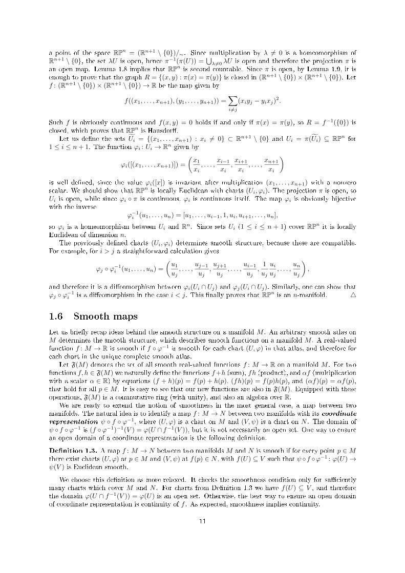
Let us dene the sets Ui = (x1, . . . , xn+1) : xi 6= 0 ⊂ Rn+1 \ 0 and Ui = π(Ui) ⊆ RPn for1 ≤ i ≤ n+ 1. The function ϕi : Ui → Rn given by

ϕi([(x1, . . . , xn+1)]) =

(x1

xi, . . . ,

xi−1

xi,xi+1

xi, . . . ,

xn+1

xi

)is well dened, since the value ϕi([x]) is invariant after multiplication (x1, . . . , xn+1) with a nonzeroscalar. We should show that RPn is locally Euclidean with charts (Ui, ϕi). The projection π is open, soUi is open, while since ϕi π is continuous, ϕi is continuous itself. The map ϕi is obviously bijectivewith the inverse

ϕ−1i (u1, . . . , un) = [u1, . . . , ui−1, 1, ui, ui+1, . . . , un],

so ϕi is a homeomorphism between Ui and Rn. Since sets Ui (1 ≤ i ≤ n + 1) cover RPn it is locallyEuclidean of dimension n.

The previously dened charts (Ui, ϕi) determines smooth structure, because these are compatible.For example, for i > j a straightforward calculation gives

ϕj ϕ−1i (u1, . . . , un) =

(u1

uj, . . . ,

uj−1

uj,uj+1

uj, . . . ,

ui−1

uj,

1

uj

uiuj, . . . ,

unuj

),

and therefore it is a dieomorphism between ϕi(Ui ∩ Uj) and ϕj(Ui ∩ Uj). Similarly, one can show thatϕj ϕ−1

i is a dieomorphism in the case i < j. This nally proves that RPn is an n-manifold. 4

1.6 Smooth maps

Let us briey recap ideas behind the smooth structure on a manifold M . An arbitrary smooth atlas onM determines the smooth structure, which describes smooth functions on a manifold M . A real-valuedfunction f : M → R is smooth if f ϕ−1 is smooth for each chart (U,ϕ) in that atlas, and therefore foreach chart in the unique complete smooth atlas.

Let F(M) denotes the set of all smooth real-valued functions f : M → R on a manifold M . For twofunctions f, h ∈ F(M) we naturally dene the functions f+h (sum), fh (product), and αf (multiplicationwith a scalar α ∈ R) by equations (f + h)(p) = f(p) + h(p), (fh)(p) = f(p)h(p), and (αf)(p) = αf(p),that hold for all p ∈M . It is easy to see that our new functions are also in F(M). Equipped with theseoperations, F(M) is a commutative ring (with unity), and also an algebra over R.

We are ready to extend the notion of smoothness in the most general case, a map between twomanifolds. The natural idea is to identify a map f : M → N between two manifolds with its coordinaterepresentation ψ f ϕ−1, where (U,ϕ) is a chart on M and (V, ψ) is a chart on N . The domain ofψ f ϕ−1 is (f ϕ−1)−1(V ) = ϕ(U ∩ f−1(V )), but it is not necessarily an open set. One way to ensurean open domain of a coordinate representation is the following denition.

Denition 1.3. A map f : M → N between two manifoldsM and N is smooth if for every point p ∈Mthere exist charts (U,ϕ) at p ∈M and (V, ψ) at f(p) ∈ N , with f(U) ⊆ V such that ψ f ϕ−1 : ϕ(U)→ψ(V ) is Euclidean smooth.

We choose this denition as more relaxed. It checks the smoothness condition only for sucientlymany charts which cover M and N . For charts from Denition 1.3 we have f(U) ⊆ V , and thereforethe domain ϕ(U ∩ f−1(V )) = ϕ(U) is an open set. Otherwise, the best way to ensure an open domainof coordinate representation is continuity of f . As expected, smoothness implies continuity.

11

Lemma 1.10. A smooth map between manifolds is continuous.

Proof. Let f : M → N be a smooth map between manifolds. For an arbitrary p ∈M there exist a chart(U,ϕ) at p ∈M and a chart (V, ψ) at f(p) ∈ N with f(U) ⊆ V , such that ψf ϕ−1 is Euclidean smooth,and therefore continuous. The restriction fU : U → V can be seen as a composition of continuous mapsψ−1 (ψ f ϕ−1) ϕ, so it is continuous itself. Since f is continuous in a neighbourhood of each pointp ∈M it is continuous on M .

Of course, the compatibility extends the smoothness condition to all charts. Let (U,ϕ) be a charton M and (V, ψ) be a chart on N . Smooth f : M → N is continuous (Lemma 1.10) which gives openf−1(V ), hence the function ψ f ϕ−1 has the open domain D = ϕ(U ∩f−1(V )). For an arbitrary pointd ∈ D 6= ∅, denote p = ϕ−1(d), so there exist charts (U1, ϕ1) at p ∈ M and (V1, ψ1) at f(p) ∈ N withf(U1) ⊆ V1 and smooth ψ1 f ϕ−1

1 . Since (ψ f ϕ−1)ϕ(U∩U1)= (ψ ψ−11 ) (ψ1 f ϕ−1

1 ) (ϕ1 ϕ−1),

while the transition maps ψ ψ−11 and ϕ1 ϕ−1 are smooth on appropriate neighbourhoods, ψ f ϕ−1 is

smooth on ϕ(U ∩U1) 3 d as a composition of smooth maps. Thus, smooth f implies smooth ψ f ϕ−1

which gives an alternative way to set a denition of smooth maps.

Lemma 1.11. A continuous map f : M → N between two manifolds M and N is smooth if and only iffor every chart (U,ϕ) on M and every chart (V, ψ) on N , the function ψ f ϕ−1 is Euclidean smooth.

Proof. We have already considered one side of a proof, so the other side remains. Let the functionψ f ϕ−1 is smooth for every chart (U,ϕ) on M and every chart (V, ψ) on N . For an arbitrary p ∈Mthere exist charts (U,ϕ) at p ∈M and (V, ψ) at f(p) ∈ N . Continuous f implies thatW = U ∩f−1(V ) isan open set, so (W,ϕW ) is a chart at p ∈M . It follows that f(W ) ⊆ V and ψf(ϕW )−1 : ϕ(W )→ ψ(V )is smooth, hence f is smooth by Denition 1.3.

Lemma 1.11 covers a more common denition of smoothness. A map f : M → N between twomanifolds is smooth if for every chart (U,ϕ) on M and every chart (V, ψ) on N , the function ψ f ϕ−1

is Euclidean smooth with the stipulation that ϕ(U ∩f−1(V )) is an open set. For example, ϕ(U ∩f−1(V ))is open if f happens to be continuous. If we allow the domain to not be open, there can arise the problemfrom the following example.

Example 1.18. The characteristic (indicator) function f : R → 0, 1 ⊂ R of the set x ∈ R : x ≥ 0,has the representation ψ f ϕ−1 = fU∩f−1(V ). Consider the single chart (R, Id) on M = R, and twocharts on N = R, for example ((−∞, 1), Id) and ((0,+∞), Id). For V = (−∞, 1), the set D = (−∞, 0)is open and ψ f ϕ−1 is constantly equal to 0, so it is smooth. However, for V = (0,+∞), the setD = [0,+∞) is not open, but ψ f ϕ−1 is constantly equal to 1 and therefore has a smooth extensionto an open set. Our goal is to generalize the denition of a smooth function between Euclidean spaces,so we do not like that such not continuous f , and therefore not ordinary smooth function, be smooth. 4

The previous example is the reason why we stipulate that ϕ(U ∩ f−1(V )) is an open set, and con-sequently require continuous f . Our denition generalizes the previous concepts. For example, a mapbetween open subsets of Euclidean spaces f : U → Rn with open U ⊆ Rm, has the coordinate represen-tation (relative to the identity charts) equal to some restriction of f , and therefore f is smooth if andonly if it is Euclidean smooth. Similarly, in the case f : M → R, we have a coincidence of smooth mapsbetween manifolds with smooth functions determined by the smooth structure.

If a restriction of map f : M → N to some neighbourhood of p ∈ M is smooth, we say that f issmooth at p. A map f is smooth if and only if f is smooth at each point in M , so the smoothness is alocal property, and the following lemma holds.

Lemma 1.12. Let M and N be manifolds and let Uαα∈Λ be a collection of open sets from M . If mapsfα : Uα → N for α ∈ Λ are smooth and for all α, β ∈ Λ holds fα = fβ on Uα ∩ Uβ, then there exists aunique smooth map f :

⋃α∈Λ → N whose restriction to Uα is equal to fα for each α ∈ Λ.

Example 1.19. The obvious example of smooth map is the identity map, or more generally the inclusionmap f : U →M for an open submanifold U ⊆M . Every constant map c : M → N is also smooth. 4

Lemma 1.13. A composition of smooth maps between manifolds is smooth.

12

Proof. Let f : M → N and h : N → P be smooth maps. Since h is smooth, for each point p ∈ Mthere exist charts (V, ψ) at f(p) ∈ N and (W, θ) at h(f(p)) ∈ P , with h(V ) ⊆ W such that θ h ψ−1 : ψ(V ) → θ(W ) is smooth. A map f is smooth, hence continuous (Lemma 1.10), so f−1(V ) is anopen neighbourhood of M at a point p, and therefore there exists a chart (U,ϕ) at p ∈ M , such thatU ⊆ f−1(V ). Since f is smooth, ψ f ϕ−1 : ϕ(U) → ψ(V ) is smooth by Lemma 1.11. Then we have(h f)(U) ⊆ h(V ) ⊆W and θ (h f) ϕ−1 = (θ h ψ−1) (ψ f ϕ−1) : ϕ(U)→ θ(W ) is smooth asa composition of smooth functions between Euclidean spaces.

Although the denition is not simple, it is often straightforward to prove that a particular map issmooth. The most common way is to write the map in local coordinates and recognize its componentfunctions as compositions of smooth elementary functions or maps that are known to be smooth.

Example 1.20. Any map from a 0-dimensional manifold into a smooth manifold is smooth, since eachcoordinate representation is constant. 4

Example 1.21. Let (U,ϕ) be a chart on an n-manifold M at a point p ∈ M . Let πi : Rn → Rfor 1 ≤ i ≤ n be the natural projections, πi(x1, . . . , xn) = xi. The coordinate functions of thechart (U,ϕ) are the functions xi : U → R dened with xi = πi ϕ for 1 ≤ i ≤ n, which means thatϕ(u) = (x1(u), . . . , xn(u)) holds for each u ∈ U . Coordinate functions are smooth since the coordinaterepresentation xi ϕ−1 is just the restriction of projection πi. 4

Example 1.22. LetM and N be manifolds and let πM : M×N →M , πM (p, q) = p be the projection tothe rst component. Let (U,ϕ) be a chart at p ∈M and (V, ψ) be a chart at q ∈ N , then (U×V, ϕ×ψ) is achart at (p, q) ∈M×N . The coordinate representation of πM is ϕπM (ϕ×ψ)−1 : (ϕ×ψ)(U×V )→ ϕ(U)given by (a1, . . . , am, b1, . . . , bn) 7→ (a1, . . . , am), which is smooth, and therefore πM is smooth. 4

Example 1.23. The height function f : Sn → R is given by f(x1, . . . , xn+1) = xn+1. Using formulasfrom Example 1.14 we can calculate

(f ϕ−1± )(y1, . . . , yn) = ∓−1 + y2

1 + · · ·+ y2n

1 + y21 + · · ·+ y2

n

,

that is smooth, and therefore f is smooth. More generally, let us consider a smooth function f : Rn+1 → Rand its restriction fSn= f i, where i : Sn → Rn+1 is the inclusion map. The inclusion map of atopological subspace is certainly continuous, its coordinate representation i ϕ−1

± : ϕ±(U±) → Rn+1 issmooth, so i is smooth and nally fSn is smooth. 4

Example 1.24 (quotient projection). The quotient map from Example 1.17, π : Rn+1 \ 0 → RPnis smooth. Its coordinate representation related to introduced coordinates for RPn and standard coordi-nates for Rn+1 \ 0 is

ϕi π Id−1(x1, . . . , xn+1) = ϕi([x1, . . . , xn+1]) =

(x1

xi, . . . ,

xi−1

xi,xi+1

xi, . . . ,

xn+1

xi

),

which is obviously smooth for (x1, . . . , xn+1) ∈ Ui, i.e. for xi 6= 0. 4

A Lie group25 is a manifold G that is also a group in the algebraic sense with the property thatthe group operations are compatible with the smooth structure. Concretely, the multiplication mapµ : G×G→ G, µ(a, b) = ab and the inversion map ı : G→ G, ı(a) = a−1 are both smooth.

Example 1.25. Let us mention basic examples of Lie groups. The Euclidean space Rn is a Lie groupunder addition. The set of nonzero complex numbers C \ 0 is a Lie group under multiplication. Theunit circle S1 in C \ 0 is a Lie group under multiplication. The product G1 × G2 of two Lie groups(G1, µ1) and (G2, µ2) is a Lie group under coordinatewise multiplication µ1 × µ2. 4

Example 1.26. The general linear group GL(n,R) = A ∈ Rn×n : detA 6= 0 from Example 1.13is a manifold as an open subset of Rn×n. Since each component of the product AB of two matricesA,B ∈ GL(n,R) is a (quadratic) polynomial in the entries of A and B, the matrix multiplication is

25Marius Sophus Lie (18421899), Norwegian mathematician

13

clearly smooth. By Cramer's26 rule, the inverse matrix A−1 is the quotient of the adjugate matrix of Aand the determinant of A. The adjugate of A is the transpose of the cofactor matrix of A, so the entriesof the inverse matrix are (degree n− 1) polynomials in the entries of A, and therefore the inversion mapis smooth. 4

A dieomorphism between manifolds M and N is a smooth bijective map f : M → N that has asmooth inverse. If such dieomorphism exists we say that M and N are dieomorphic. A dieomor-phism of manifolds is a bijection of the underlying sets that identies the complete smooth atlases of themanifolds. Similarly, a homeomorphism between manifolds M and N is a continuous bijective mapf : M → N that has a continuous inverse, and we say that manifolds are homeomorphic. Since everysmooth map is continuous, every dieomorphism is a homeomorphism.

The manifold theory investigates properties of manifolds that are preserved by dieomorphisms, so wecan consider dieomorphic manifolds to be the same. Manifolds that are homeomorphic are consideredthe same topologically.

Example 1.27. If f is an injective map from a set P onto a manifold M , then there is a uniqueway to make P a manifold (a unique topology and a complete smooth atlas on P ) such that f is adieomorphism. The topology on P is determined by sets f−1(U) where U is an open subset ofM , whilesmooth atlas on P consists of charts (f−1(U), ϕ f) where (U,ϕ) is a chart on M . 4

Example 1.28. Let Mn be a manifold. Every chart (U,ϕ) on a manifold M gives a dieomorphismϕ : U → ϕ(U) from the open submanifold U ⊆ M onto an open subset of Rn. To check the smoothnessof ϕ and ϕ−1 we can use the chart (U,ϕ) on U and the chart (ϕ(U), Idϕ(U)) on ϕ(U), where we have

that Idϕ(U) ϕ ϕ−1 = Idϕ(U) = ϕ ϕ−1 Id−1ϕ(U) is smooth, so ϕ and ϕ−1 are smooth. Conversely, every

dieomorphism f : U → f(U) from an open subset U ⊆ M onto an open subset of Rn is a chart in thecomplete smooth atlas. Namely, if (V, ψ) is a chart on M , we have already know that both, ψ and ψ−1

are smooth, so by Lemma 1.13 the transition maps f ψ−1 and ψ f−1 are smooth, and any chart iscompatible with (U, f). 4

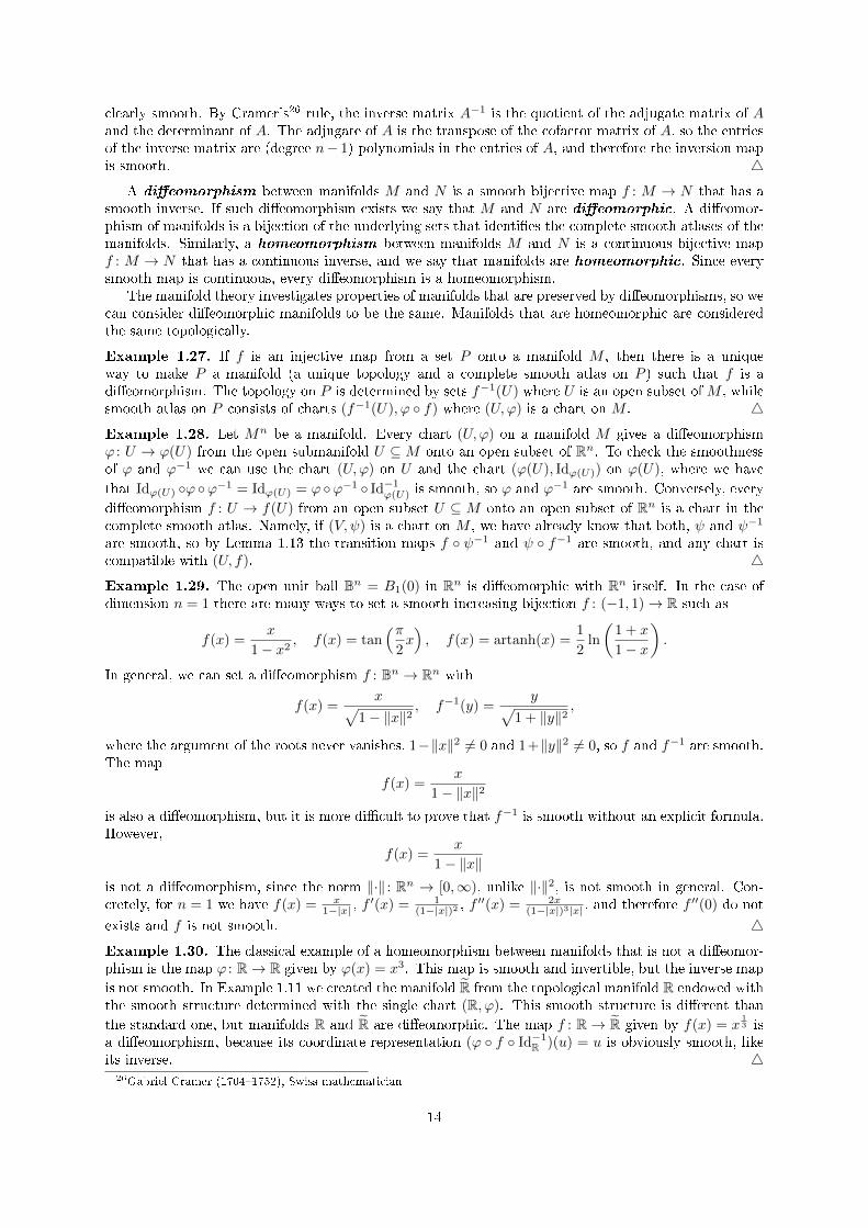
Example 1.29. The open unit ball Bn = B1(0) in Rn is dieomorphic with Rn itself. In the case ofdimension n = 1 there are many ways to set a smooth increasing bijection f : (−1, 1)→ R such as

f(x) =x

1− x2, f(x) = tan

(π2x), f(x) = artanh(x) =

1

2ln

(1 + x

1− x

).

In general, we can set a dieomorphism f : Bn → Rn with

f(x) =x√

1− ‖x‖2, f−1(y) =

y√1 + ‖y‖2

,

where the argument of the roots never vanishes, 1−‖x‖2 6= 0 and 1+‖y‖2 6= 0, so f and f−1 are smooth.The map

f(x) =x

1− ‖x‖2

is also a dieomorphism, but it is more dicult to prove that f−1 is smooth without an explicit formula.However,

f(x) =x

1− ‖x‖is not a dieomorphism, since the norm ‖·‖ : Rn → [0,∞), unlike ‖·‖2, is not smooth in general. Con-cretely, for n = 1 we have f(x) = x

1−|x| , f′(x) = 1

(1−|x|)2 , f′′(x) = 2x

(1−|x|)3|x| , and therefore f ′′(0) do not

exists and f is not smooth. 4

Example 1.30. The classical example of a homeomorphism between manifolds that is not a dieomor-phism is the map ϕ : R→ R given by ϕ(x) = x3. This map is smooth and invertible, but the inverse map

is not smooth. In Example 1.11 we created the manifold R from the topological manifold R endowed withthe smooth structure determined with the single chart (R, ϕ). This smooth structure is dierent than

the standard one, but manifolds R and R are dieomorphic. The map f : R→ R given by f(x) = x13 is

a dieomorphism, because its coordinate representation (ϕ f Id−1R )(u) = u is obviously smooth, like

its inverse. 426Gabriel Cramer (17041752), Swiss mathematician

14

Example 1.31. LetM be a manifold with a complete smooth atlas A. Any homeomorphism f : M →Mdetermines a new atlas A′ onM with charts (f(U), ϕf−1) ∈ A′ obtained from charts (U,ϕ) ∈ A. Thenf is a dieomorphism if and only if A = A′. Therefore, if f is a homeomorphism which is not adieomorphism, then f denes a new atlas A′ 6= A. However, the new smooth structure on M isnot essentially dierent from the old one. Although f : M → M is not a dieomorphism it denesa dieomorphism between M and the manifold with the atlas A′. Hence, even though A and A′ aredierent atlases, the resulting smooth structures are still dieomorphic. 4

Unlike non-dieomorphic homeomorphisms, it is dicult to nd two homeomorphic manifolds thatare not dieomorphic. It turns out that every topological n-manifold for n ≤ 3 has a smooth structurethat is unique up to dieomorphism (see Moise27 [51]). However, the rst example of exotic manifoldstructures was discovered by Milnor28 in 1956 [50], who found that 7-sphere S7 admits manifold structuresthat are not dieomorphic to the standard manifold structure.

It is an interesting question whether a given topological manifold can carry smooth structures thatare not dieomorphic. This question is very complicated, even for Euclidean spaces. It appears thatRn for n 6= 4 has a unique smooth structure, up to dieomorphism (see Stallings29 [65]). However, acombination of results due to Donaldson30 [26] and Freedman31 [29] led to the discovery of non-standardsmooth structures on R4. Moreover, R4 has uncountably many distinct smooth structures, no two ofwhich are dieomorphic to each other (see Taubes32 [66]).

On the other hand, there exist topological manifolds that do not admit smooth structures at all. Therst example of this deep result was a compact 10-dimensional manifold found by Kervaire33 in 1960[44]. In fact, examples of non-smoothable n-topological manifolds are known for each n ≥ 4. The mostfamous example is so-called E8 manifold, which is a 4-topological manifold discovered by Freedman in1982 [29].

1.7 Partitions of unity

Since manifolds are constructed by gluing open sets in Rn by dieomorphisms, it can be a tricky matterwhen we are doing things all over a manifold. The theory of partitions of unity is important, thoughtechnical, tool that allows us work in local coordinates. It is a way of breaking the function with theconstant value 1 into a bunch of smooth pieces that will be easier to work with.

The support of a function f : M → R is the closure of the set of points where f is nonzero, supp(f) =p ∈M : f(p) 6= 0. Clearly, the complement of supp(f) is the largest open set on which f is identicallyzero. If supp(f) is contained in some set U ⊆M , we say that f is supported in U .

There is a huge number of smooth functions on a manifold, but the heart of partitions of unity arethe bump functions. These are smooth equivalents of characteristic functions, and we use them to maska function f . If we multiply f by a characteristic function of U , the result is supported in U , but thiscauses some discontinuities. A bump function b repairs the problem by smoothly decreasing to zerobetween an inner set V and an outer open set U ⊇ V . For x ∈ V we have b(x) = 1 and therefore(fb)(x) = f(x), while for x /∈ U we have (fb)(x) = 0. Additionally, the product fb will be at least assmooth as f was, except in the case of analytic functions. The core of the theory is a function with theproperties from the following lemma.

Lemma 1.14. There exists a smooth function f : R → R that vanishes for all negative values of thedomain and is strictly positive for its positive values.

Proof. Let us start with the famous non-analytic smooth function f : R→ R dened by

f(x) =

e−

1x if x > 0,

0 if x ≤ 0,(1.1)

27Edwin Evariste Moise (19181998), American mathematician28John Willard Milnor (1931), American mathematician29John Robert Stallings Jr. (19352008), American mathematician30Simon Kirwan Donaldson (1957), English mathematician31Michael Hartley Freedman (1951), American mathematician32Cliord Henry Taubes (1954), American mathematician33Michel Andre Kervaire (19272007), French mathematician

15

that has wanted properties. For x < 0 it is obviously f (n)(x) = 0. For x > 0 we can use the inductionover n to prove that the n-th derivative of the function f has the form

f (n)(x) =Pn(x)

x2nf(x), (1.2)

where Pn(x) is a polynomial of degree n − 1. The induction basis n = 1 gives f ′(x) = 1x2 f(x) and

therefore P1(x) = 1. The induction step follows

f (n+1)(x) =

(P ′n(x)

x2n− 2n

Pn(x)

x2n+1+Pn(x)

x2n+2

)f(x) =

x2P ′n(x)− (2nx− 1)Pn(x)

x2n+2f(x) =

Pn+1(x)

x2(n+1)f(x),

where Pn+1(x) is a polynomial of degree n, with the recursion Pn+1(x) = x2P ′n(x)− (2nx− 1)Pn(x).It remains to show that the right-hand side derivative of f at x = 0 is zero. The exponential dominates

the powers of x > 0, for example for all m ∈ N0 we have

1

xm= x

(1

x

)m+1

≤ (m+ 1)!x

∞∑i=0

1

i!

(1

x

)i= (m+ 1)!xe

1x ,

and therefore

limx0

e−1x

xm≤ (m+ 1)! lim

x0x = 0. (1.3)

Using (1.3) for m = 1, we see that

f ′(0) = limx0

f(x)− f(0)

x− 0= limx0

e−1x

x= 0.

Since (1.2) is established for x > 0, the limit (1.3) for m = 2n+ 1, with the assumption that f (n)(0) = 0,implies

f (n+1)(0) = limx0

f (n)(x)− f (n)(0)

x− 0= limx0

Pn(x)

x2n+1e−

1x = 0,

which by induction over n proves that f (n)(0) = 0 for every n ∈ N, and therefore f is smooth.Additionally, one can notice that the function f is not analytic at zero. Since f (n)(0) = 0 holds for

all n ∈ N0, the Maclaurin34 series of f converges everywhere to the zero function, but it is not equal tof(x) for x > 0.

Lemma 1.14 allows us to create a so-called cuto function .

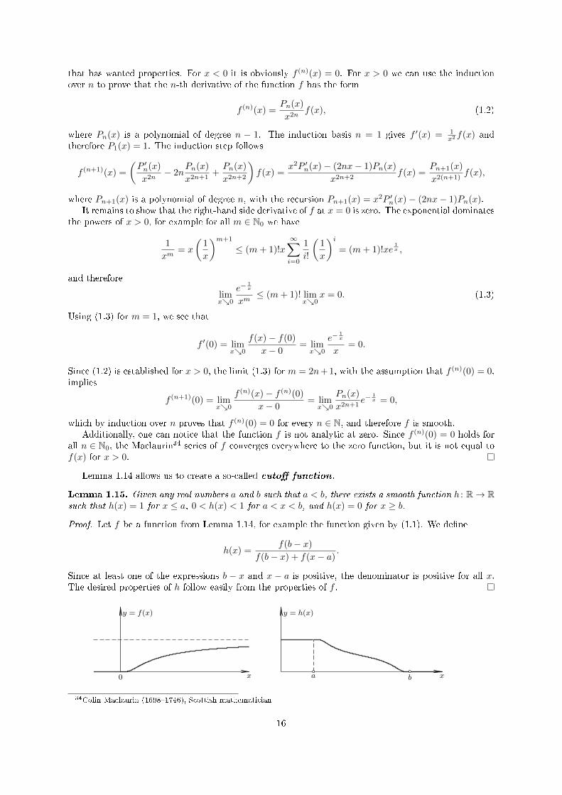
Lemma 1.15. Given any real numbers a and b such that a < b, there exists a smooth function h : R→ Rsuch that h(x) = 1 for x ≤ a, 0 < h(x) < 1 for a < x < b, and h(x) = 0 for x ≥ b.

Proof. Let f be a function from Lemma 1.14, for example the function given by (1.1). We dene

h(x) =f(b− x)

f(b− x) + f(x− a).

Since at least one of the expressions b − x and x − a is positive, the denominator is positive for all x.The desired properties of h follow easily from the properties of f .

0 x

y = f(x)

a b x

y = h(x)

34Colin Maclaurin (16981746), Scottish mathematician

16

Lemma 1.15 can be generalized in Rn where we use the open balls Br(p) = x ∈ Rn : ‖x− p‖ < r.

Lemma 1.16. Given any a, b ∈ R such that 0 < a < b, there exists a smooth function f : Rn → R suchthat f(x) = 1 for x ∈ Ba(0), 0 < f(x) < 1 for x ∈ Bb(0) \Ba(0), and f(x) = 0 for x ∈ Rn \Bb(0).

Proof. Let us set the function f : Rn → R with f(x) = h(‖x‖), where h is the function from Lemma1.15. The function f is smooth on Rn \ 0, because it is a composition of smooth functions there. It isidentically equal to 1 on Ba(0), and therefore it is also smooth at the origin.

This concept can be generalized for manifolds.

Lemma 1.17. Let M be a manifold and U be some open neighbourhood of p ∈ M . Then there is asmooth function f : M → [0, 1] ⊆ R that is identically equal to 1 on some neighbourhood of V 3 p andalso supported in U ⊇ V .

Proof. By Lemma 1.7, starting from an arbitrary map (Y, ψ) in p ∈ Mn, we can use an appropriatecomposition of homothety and translation in Rn for a dieomorphism and W = U ∩ Y for a restriction,to construct a chart (W,ϕ) centred at p ∈ M (ϕ(p) = 0) such that B3(0) ⊆ ϕ(W ). Let b : Rn → R bea smooth function from Lemma 1.16 with b(x) = 1 for ‖x‖ ≤ 1, 0 < b(x) < 1 for 1 < ‖x‖ < 2, andb(x) = 0 for ‖x‖ ≥ 2. A new function f = b ϕ : W → [0, 1] ⊆ R is smooth and satises f(x) = 0 forx /∈ ϕ−1(B2(0)) ⊆ W . We want to dene f for points from M \W , so we use the zero function denedon M \ ϕ−1(B2(0)), and apply Lemma 1.12 to get f ∈ F(M). The function f is equal to 1 on the openneighbourhood V = ϕ−1(B1(0)) 3 p and it is supported in U ⊇W ⊇ V .

The function f ∈ F(M) from Lemma 1.17 is called a bump function at p and it easily extends asmooth function on the whole manifold M .

Lemma 1.18. Let M be a manifold and U be some open neighbourhood of p ∈ M . If f : U → R issmooth then there exist an open neighbourhood V 3 p with V ⊆ U and a function in F(M) that agreeswith f on V and vanishes outside of U .

Proof. Let b ∈ F(M) be a bump function from Lemma 1.17 which is identically equal to 1 on some openneighbourhood V 3 p and supported in U ⊇ V . If we join the function bf dened on U and the zerofunction dened on M \ V ⊇ M \ U , using Lemma 1.12 we get a function that satises the requiredproperty.

Lemma 1.19. Let K be compact and U ⊇ K be an open subset of a manifold M . Then there is a smoothfunction f : M → [0, 1] ⊆ R supported in U which is equal to 1 on K.

Proof. According to Lemma 1.17, for every p ∈ K ⊆ U ⊆M there exist an open set Vp 3 p and a smoothfunction fp : M → [0, 1] ⊆ R supported in U such that fpVp= 1. The collection Vpp∈K is an open coverof compact K and therefore it has a nite subcover Vp1 , . . . , Vpk. The function f : M → [0, 1] ⊆ Rgiven by f = 1 − (1 − fp1)(1 − fp2) · · · (1 − fpk) is clearly supported in U . Moreover f is equal to 1 oneach Vpi for 1 ≤ i ≤ k, and therefore 1 on the whole K ⊆

⋃ni=1 Vpi .

A partition of unity is a decomposition∑α∈Λ fα = 1 of constant function 1 (the word unity stands

for this function) into a sum of smooth functions fα. We usually deal with innite sums, so our functionsare indexed by some innite set Λ, so it is natural to require that for each p ∈M we have fα(p) = 0 forall but a nite number of α ∈ Λ. The sum is then well dened as a function on M and we can retain thesmoothness through the following denition.

Denition 1.4. A partition of unity on a manifold M is a collection fαα∈Λ of smooth func-tions fα : M → [0, 1] ⊆ R, such that the collection of supports supp(fα)α∈Λ is locally nite and∑α∈Λ fα(p) = 1 holds for all p ∈ M . We say that a partition of unity is subordinate to some cover of

M if the collection of all supports is a renement of this cover.

This denition implies that for every p ∈ M there exists some α ∈ Λ such that fα(p) > 0, and thussupp(fα)α∈Λ is a cover of M . This cover is locally nite, so the (innite) sum

∑α∈Λ fα(p) is well

dened. If Uαα∈Λ is a cover of M and supp(fα) ⊆ Uα holds for all α ∈ Λ, then we say that fαα∈Λ

is subordinate to Uαα∈Λ with the same index set as the partition of unity. However, if fαα∈Λ is apartition of unity subordinate to a cover Vββ∈∆, then supp(fα)α∈Λ is a renement of Vββ∈∆ andwe can use the renement map φ : Λ → ∆ satisfying supp(fα) ⊆ Vφ(α) for every α ∈ Λ, and get thepartition of unity

∑α∈φ−1(β) fαβ∈∆ that is subordinate to Vββ∈∆ with the same index set.

17

Theorem 1.20. For any open cover of a manifold there exists a partition of unity subordinate to it.

Proof. Let U be an open cover ofM . SinceM is locally compact (Lemma 1.1) there is an open renementU ′ of U consists of open sets whose closure is compact. Then, because M is paracompact (Theorem 1.5)we may nd a new open renement V of U ′ which is locally nite.

Consider the set W = U ⊆ M : U is open and U ⊆ V for some V ∈ V. Every point p ∈ M has aneighbourhood V ∈ V, and since M is regular (Theorem 1.4), the point p and the closed set M \ V 63 pare separated by some open disjoint sets P 3 p and Q ⊇M \V . Because of P ∩Q = ∅ we have P ⊆M \Q,so P ⊆M \Q, while M \ V ⊆ Q implies M \Q ⊆ V , and therefore P ⊆M \Q ⊆ V . Hence p ∈ P ∈ W,which means that W is a cover of M , and therefore it is an open renement of V.

Another use of paracompactness gives a locally nite open renement W ′ of W. The collectionW ′ = Wββ∈∆ ⊆ W is a renement of V = Vαα∈Λ and for each β ∈ ∆ there is φ(β) ∈ Λ such thatWβ ⊆ Vφ(β), which denes φ : ∆→ Λ and we can set Xα =

⋃β∈φ−1(α)Wβ (by convention it is the empty

set in a case of φ−1(α) = ∅).

SinceW ′ is a locally nite collection, for every p ∈M \⋃β∈IWβ there is a neighbourhood U 3 p which

intersects just nite number of members, for example W1, . . . ,Wk. For other Wi we have Wi ∩U = ∅, itimplies Wi ⊆M \U , soWi ⊆M \U and thereforeWi∩U = ∅. Hence U \

⋃β∈IWβ = U \ (W1∪· · ·∪Wk)

is an open neighbourhood of p, which means that M \⋃β∈IWβ is open, so

⋃β∈IWβ is closed and⋃

β∈IWβ =⋃β∈IWβ holds.

Now, we have Xα =⋃β∈φ−1(α)Wβ =

⋃β∈φ−1(α)Wβ ⊆ Vα, so for any α ∈ Λ we have compact Xα

contained in open Vα, and by Lemma 1.19 there is a smooth function fα ∈ F(M) supported in Vα andequal to 1 on Xα. The sum f =

∑α∈Λ fα is a smooth function which is always nite non-zero. Therefore,

the sum of new functions fα/f is 1 everywhere.

1.8 Tangent vectors

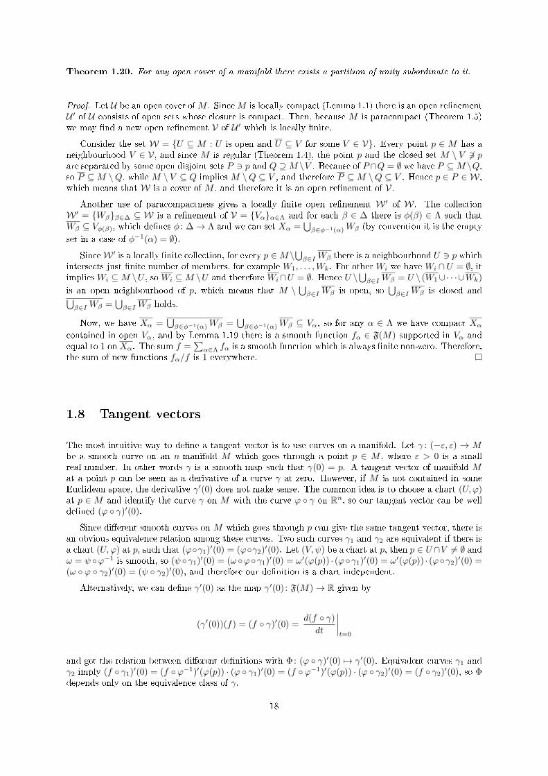
The most intuitive way to dene a tangent vector is to use curves on a manifold. Let γ : (−ε, ε) → Mbe a smooth curve on an n-manifold M which goes through a point p ∈ M , where ε > 0 is a smallreal number. In other words γ is a smooth map such that γ(0) = p. A tangent vector of manifold Mat a point p can be seen as a derivative of a curve γ at zero. However, if M is not contained in someEuclidean space, the derivative γ′(0) does not make sense. The common idea is to choose a chart (U,ϕ)at p ∈ M and identify the curve γ on M with the curve ϕ γ on Rn, so our tangent vector can be welldened (ϕ γ)′(0).

Since dierent smooth curves on M which goes through p can give the same tangent vector, there isan obvious equivalence relation among these curves. Two such curves γ1 and γ2 are equivalent if there isa chart (U,ϕ) at p, such that (ϕγ1)′(0) = (ϕγ2)′(0). Let (V, ψ) be a chart at p, then p ∈ U∩V 6= ∅ andω = ψ ϕ−1 is smooth, so (ψ γ1)′(0) = (ω ϕγ1)′(0) = ω′(ϕ(p)) · (ϕγ1)′(0) = ω′(ϕ(p)) · (ϕγ2)′(0) =(ω ϕ γ2)′(0) = (ψ γ2)′(0), and therefore our denition is a chart independent.

Alternatively, we can dene γ′(0) as the map γ′(0) : F(M)→ R given by

(γ′(0))(f) = (f γ)′(0) =d(f γ)

dt

∣∣∣∣t=0

and get the relation between dierent denitions with Φ: (ϕ γ)′(0) 7→ γ′(0). Equivalent curves γ1 andγ2 imply (f γ1)′(0) = (f ϕ−1)′(ϕ(p)) · (ϕ γ1)′(0) = (f ϕ−1)′(ϕ(p)) · (ϕ γ2)′(0) = (f γ2)′(0), so Φdepends only on the equivalence class of γ.

18

ϕ(U)

ϕ

p

U

f(p)

Rε

−ε

0 γf

ϕ γ

f ϕ−1

Although such denition of a tangent vector is very geometric, it has disadvantages. Namely, it isnot instantly obvious where the vector space structure comes from, and it does not generalize well toalgebraic varieties.

Because of (αf + βh) γ = α(f γ) + β(h γ), an evident property of the function γ′(0) is linearity.From the other side, since (fh) γ = (f γ)(h γ) holds, we have

(γ′(0))(fh) = ((fγ)(hγ))′(0) = (fγ)′(0)·h(γ(0))+(hγ)′(0)·f(γ(0)) = h(p)(γ′(0))(f)+f(p)(γ′(0))(h),

which means that γ′(0) satises the Leibniz35 law (product rule). Hence, γ′(0) has properties character-istic for the derivative (an R-linear function which is Leibnizian at p), so a real-valued function on F(M)with this features we call the derivation at point p. The showed properties for γ′(0) motivate us toocially introduce the denition of a tangent vector.

A tangent vector to a manifold M at a point p ∈ M is a derivation at p, X : F(M) → R. The setTpM of all tangent vectors on a manifold M at a point p ∈ M is called the tangent space to M atp. Accordingly, if X ∈ TpM , then for all α, β ∈ R and every f, h ∈ F(M) hold linearity X(αf + βh) =αX(f) + βX(h) and Leibnizian X(fh) = f(p)X(h) + h(p)X(f).

Moreover, we dene the addition and the scalar multiplication naturally. If X,Y ∈ TpM then(X + Y )(f) = X(f) + Y (f) and (αX)(f) = αX(f) hold for each f ∈ F(M) and all α ∈ R. Such denedX + Y and αX are also tangent vectors and thus TpM is a vector space over R.

By their very nature manifolds are curved spaces, and they can be very complicated objects to study,while vector spaces are much simpler with many benets. A tangent space TpM is a vector space, andit can be thought of as the best linear approximation to a manifold M at a point p ∈ M . This is thereason why we are minded to use a tangent space instead of an original manifold.

Naturally, the derivative of a constant function vanishes.

Lemma 1.21. If f ∈ F(M) is constant, then X(f) = 0 holds for every X ∈ TpM .

Proof. From the Leibnizian condition we have X(1) = X(1 · 1) = 1(p)X(1) + 1(p)X(1) = 2X(1) andtherefore X(1) = 0, where 1 ∈ F(M) is the constant unit function. For α ∈ R, linearity gives X(α1) =αX(1) = 0.

The tangent space is dened in terms of smooth functions on the whole manifold, while charts are ingeneral dened on some open subsets. However, tangent vectors act locally on F(M).

Lemma 1.22. Let M be a manifold, p ∈ M , X ∈ TpM , and f, h ∈ F(M). If f and h agree on someneighbourhood of p, then X(f) = X(h).

35Gottfried Wilhelm von Leibniz (16461716)

19

Proof. Let f = h on some neighbourhood U 3 p. By Lemma 1.17 there exist a neighbourhood V 3 pand a smooth function b ∈ F(M) such that b is 1 on V and 0 outside of U . Then (f − h)b = 0 on all ofM , hence 0 = X((f − h)b) = b(p)X(f − h) + (f − h)(p)X(b) = X(f − h) and thus X(f) = X(h).

The previous lemma is very important, because it allows the notion of germs. Two functions f : U → Rand h : V → R, locally dened on some neighbourhoods of p ∈ M , are equivalent if there exists someopen subset W ⊆ U ∩ V , containing p, so that fW= hW . The equivalence class of such functions iscalled a germ at p.

Since we work with smooth functions (instead of Ck functions with k < ∞), any locally denedsmooth function by Lemma 1.18 has an equivalent smooth function dened on the whole manifold M .Let us notice that if f and h are extensions of equivalent smooth functions, by Lemma 1.22 we haveX(f) = X(h) for any X ∈ TpM . Thus, a tangent vector X ∈ TpM is essentially dened on the germ atp, so we also use the notation X(f) for functions f ∈ F(U) where U 3 p is an open subset of M , whichtakes the value of X in an arbitrary (thus, each) function in F(M) that is equivalent to f in p.

To dene partial dierentiation on a manifold, we should move the function f back to the Euclideanspace using some chart, and then take the usual partial derivatives. Let (U,ϕ) be a chart on an n-manifold M at a point p ∈ M , and xi = πi ϕ for 1 ≤ i ≤ n are appropriate coordinate functions. Thepartial derivative of a function f ∈ F(M) for 1 ≤ i ≤ n we dene by

(∂i)p(f) =

(∂

∂xi

)p

(f) =∂f

∂xi(p) =

∂(f ϕ−1)

∂πi(ϕ(p)).

Since our denition comes from a derivative we immediately have linearity and the Leibniz's law, so suchdened function (∂i)p : F(M) → R is a tangent vector to M at p. Moreover, these partial derivativesform a basis of our tangent space TpM . To prove this we use the following simple, but fundamentalstatement, known as the Hadamard's lemma36.

Lemma 1.23. Let f be a smooth real-valued function dened on an open convex neighbourhood U 3 ain Rn. Then f(x) for all x ∈ U can be expressed in the form

f(x) = f(a) +

n∑i=1

(πi(x)− πi(a))li(x), (1.4)

where li ∈ F(U) for 1 ≤ i ≤ n.

Proof. If we dene h : [0, 1]→ R by h(t) = f(a+ t(x− a)), then since

h′(t) =

n∑i=1

∂f

∂πi(a+ t(x− a))(πi(x)− πi(a)),

we have

f(x)− f(a) = h(1)− h(0) =

∫ 1

0

h′(t) dt =

n∑i=1

(πi(x)− πi(a))

∫ 1

0

∂f

∂πi(a+ t(x− a)) dt,

so if we let li =∫ 1

0∂f∂πi

(a+ t(x− a)) dt we have proven the lemma.

Hadamard's lemma is essentially a rst-order form of Taylor's theorem37. By iterating the expansion(1.4) we arrive at a second-order form,

f(x) = f(a) +

n∑i=1

(πi(x)− πi(a))

li(a) +

n∑j=1

(πj(x)− πj(a))lij(x)

= f(a) +

n∑i=1

(πi(x)− πi(a))∂f

∂πi(a) +

n∑i,j=1

(πi(x)− πi(a))(πj(x)− πj(a))lij(x), (1.5)

36Jacques Salomon Hadamard (18651963), French mathematician37Brook Taylor (16851731), English mathematician

20

where lij ∈ F(U).Let (U,ϕ) be a chart at p ∈M such that ϕ(U) is convex (for instance, an open ball), and let f ∈ F(U).

If we apply (1.5) for the smooth function f ϕ−1 ∈ F(ϕ(U)) and points a = ϕ(p) and x = ϕ(q), we get

f(q) = f(p) +

n∑i=1

(xi(q)− xi(p))∂(f ϕ−1)

∂πi(ϕ(p)) +

n∑i,j=1

(xi(q)− xi(p))(xj(q)− xj(p))lij(q),

where lij(q) is smooth for 1 ≤ i, j ≤ n.Let us examine X(f) for an arbitrary tangent vector X ∈ TpM . The rst term f(p) is constant, so

it vanishes by Lemma 1.21. The Leibnizian property implies that X vanishes the last sum since eachof three obtained terms has at least one factor of the form (xi(q) − xi(p))(p) = 0. It remains the sumin the middle, where X(f) = X(

∑ni=1(xi(q) − xi(p))(∂i)p(f)) =

∑ni=1X(xi)(∂i)p(f), and therefore we

have X =∑ni=1X(xi)(∂i)p, which means that the partial derivatives (∂i)p generate the tangent space

TpM .If we apply these partial derivatives on the coordinate functions we get (∂i)p(xj) = δij . Then∑ni=1 λi(∂i)p = 0 implies λj = (λ1(∂1)p + · · · + λn(∂n)p)(xj) = 0 for all 1 ≤ j ≤ n, and therefore

(∂1)p, . . . , (∂n)p are linearly independent. This proves the following basis theorem.

Theorem 1.24. Let Mn be a manifold and (U,ϕ) be a chart at p ∈M with xi = πi ϕ. Then the partialderivatives (∂1)p, . . . , (∂n)p form a basis of TpM and X =

∑ni=1X(xi)(∂i)p holds for all X ∈ TpM .

Let us go back to the beginning where we had a smooth curve γ : (−ε, ε) → M , a chart (U,ϕ) atp = γ(0) and the relation Φ: (ϕ γ)′(0) 7→ γ′(0) which does not depend of the choice of an equivalentcurve. We have already seen that γ′(0) is a derivation at p, which means that γ′(0) ∈ TpM .

The map Φ is injective since (ϕ γ1)′(0) 6= (ϕ γ2)′(0) means that there exists some 1 ≤ i ≤ n suchthat (πiϕγ1)′(0) 6= (πiϕγ2)′(0), respectively (γ′1(0))(xi) 6= (γ′2(0))(xi), and therefore γ′1(0) 6= γ′2(0).The map Φ is also surjective since any X ∈ TpM , by Theorem 1.24, has the form X =

∑ni=1 λi(∂i)p

for some λ1, . . . , λn ∈ R and for small ε > 0 we can construct the curve γ : (−ε, ε) → M with γ(t) =ϕ−1(ϕ(p)+t(λ1, . . . , λn)), wor which it is (γ′(0))(f) = (f γ)′(0) = (f ϕ−1)′(ϕ(p))·(λ1, . . . , λn) = X(f).By this we have shown that TpM can be identied with the equivalence classes of smooth curves whichgo through the point p ∈M ,

1.9 Tangent maps

The basic idea of dierential calculus is to approximate smooth objects by linear objects. The tangentspace TpM is a linear approximation of a manifold M at point p ∈M . The next idea is to approximatea smooth map f : M → N between manifolds by a linear transformation of tangent spaces.

For X ∈ TpM and h ∈ F(N) we can naturally set (Tpf(X))(h) = X(h f). It is easy to see that suchdened map Tpf(X) : F(N)→ R is linear. Moreover, it is Leibnizian, since for h1, h2 ∈ F(N) we have

Tpf(X)(h1h2) = X((h1h2) f) = X((h1 f)(h2 f)) = h1(f(p))X(h2 f) + h2(f(p)))X(h1 f)

= h1(f(p))Tpf(X)(h2) + h2(f(p))Tpf(X)(h1).

Thus Tpf(X) is a derivation at f(p) ∈ N , which gives Tpf(X) ∈ Tf(p)N .This way, for any smooth map f : M → N between manifolds, we dene the tangent map of f at a

point p ∈ M with Tpf : TpM → Tf(p)N and Tpf(X)(h) = X(h f), where X ∈ TpM and h ∈ F(N). Itis straightforward that the tangent map is linear. Let us notice that the tangent map Tpf is also calledthe dierential of f at p, and it is sometimes denoted by dfp, f

′p, or Dpf .

Example 1.32. The tangent map of the identity IdM : M →M at some point p ∈M is the identity mapIdTpM : TpM → TpM since for X ∈ TpM and f ∈ F(M) we have ((Tp(IdM ))(X))(f) = X(f IdM ) =X(f). 4

The chain rule can easily be generalized to manifolds, which gives that the tangent map of compositionis the composition of tangent maps.

Theorem 1.25. Given any two smooth maps f : M → N and h : N → P between manifolds, for eachpoint p ∈M we have Tp(h f) = Tf(p)h Tpf .

21

Proof. If f : M → N and h : N → P are smooth maps between manifolds, p ∈ M and X ∈ TpM , thenfor l ∈ F(N) we have

Tp(h f)(X)(l) = X(l h f) = Tpf(X)(l h) = (Tf(p)h(Tpf(X)))(l),

which proves the statement.

Theorem 1.26. Let f : M → N be a dieomorphism between manifolds and p ∈M , then Tpf : TpM →Tf(p)N is an isomorphism between vector spaces and holds (Tpf)−1 = Tf(p)(f

−1).

Proof. Since f : M → N and f−1 : N →M are smooth maps, by Theorem 1.25 we have both, IdTpM =Tp(IdM ) = Tp(f

−1 f) = Tf(p)(f−1) Tpf and IdTf(p)M = Tf(p)(IdN ) = Tf(p)(f f−1) = Tpf

Tf(p)(f−1).

Example 1.33. Let us consider the important special case when a smooth map between manifolds isa function f ∈ F(M), which means N = R. If (U,ϕ) is a chart at p ∈ M , it is enough to calculate thetangent map Tpf on the basis vectors (∂1)p, . . . , (∂n)p of the tangent space TpM . Then, for h ∈ F(R) wehave

Tpf((∂i)p)(h) =

(∂

∂xi

)p

(h f) =∂(h f ϕ−1)

∂πi(ϕ(p)).

There is just one coordinate function on R, which we often denote by t, while a basis vector at Tf(p)Rassociated to this coordinate is ( ddt )f(p). Using the chain rule, we nd that

Tpf((∂i)p)(h) = h′(f(p)) · ∂(f ϕ−1)

∂πi(ϕ(p)) =

(∂

∂xi

)p

f ·(d

dt

)f(p)

h,

therefore Tpf((∂i)p) = (∂i)p(f)( ddt )f(p), and by linearity we have

Tpf(X) = X(f)

(d

dt

)f(p)

.

4

Let Mm and Nn be manifolds, and f : M → N be a smooth map. We want to explore the tangentmap in coordinates. Let (U,ϕ) be a chart at p ∈ M with xj = πj ϕ for 1 ≤ j ≤ m, and (V, ψ) be achart at f(p) ∈ N with yi = πi ψ for 1 ≤ i ≤ n. According to Theorem 1.24, for each 1 ≤ j ≤ m wehave

Tpf

(∂

∂xj

)p

=

n∑i=1

(Tpf

(∂

∂xj

)p

)(yi)

(∂

∂yi

)f(p)

=

n∑i=1

∂(yi f)

∂xj(p)

(∂

∂yi

)f(p)

. (1.6)

The matrix of the tangent map Tpf with respect to these coordinate bases is(∂(yi f)

∂xj(p)

)1≤i≤n, 1≤j≤m

called the Jacobian matrix of f at p relative to charts ϕ and ψ. Especially, if we put f = IdM : M →M ,then we have (

∂

∂xj

)p

=

n∑i=1

∂yi∂xj

(p)

(∂

∂yi

)p

, (1.7)

which gives the rule for the change of coordinates, and the Jacobian matrix here is related to the transitionmap ψ ϕ−1 at ϕ(p).

Example 1.34. The transition map between polar coordinates and standard coordinates in suitable opensubsets of the plane is given by (x, y) = (r cos θ, r sin θ). Let p ∈ R2 has polar coordinates (r, θ) = (3, π2 )

22

and let X ∈ TpR2 be the tangent vector whose polar coordinate representation is X = 2( ∂∂r )p − ( ∂∂θ )p.Concrete calculations by the formula (1.7) give(

∂

∂r

)p

=∂x

∂r(p)

(∂

∂x

)p

+∂y

∂r(p)

(∂

∂y

)p

= cos(π

2

)( ∂

∂x

)p

+ sin(π

2

)( ∂

∂y

)p

=

(∂

∂y

)p(

∂

∂θ

)p

=∂x

∂θ(p)

(∂

∂x

)p

+∂y

∂θ(p)

(∂

∂y

)p

= −3 sin(π

2

)( ∂

∂x

)p

+ 3 cos(π

2

)( ∂

∂y

)p

= −3

(∂

∂x

)p

,

and therefore X = 2( ∂∂r )p − ( ∂∂θ )p = 3( ∂∂x )p + 2( ∂∂y )p. 4

Lemma 1.27. Let U ⊆M be an open subset with the inclusion ı : U →M . For each p ∈ U , the tangentmap Tpı : TpU → TpM is an isomorphism.

Proof. To prove injectivity of the map Tpı, suppose Tpı(X) = 0 ∈ TpM for some X ∈ TpU . For anarbitrary f ∈ F(U), by Lemma 1.18 there is an extension f ∈ F(M) supported in U which agreeswith f on some open neighbourhood of p, so X(f) = X(fU ) = X(f ı) = ((Tpı)(X))(f) = 0. SinceX(f) = 0 holds for any f ∈ F(U) then X = 0 and Tpı is injective. To prove surjectivity, supposeY ∈ TpM is arbitrary. For f ∈ F(U), as before, there is an extension f ∈ F(M) and we can deneX : F(U) → R with X(f) = Y (f), while it is easy to check X ∈ TpU . For any f ∈ F(M) we have(Tpı(X))(f) = X(f ı) = Y (f ı) = Y (f), so Tpı is surjective.

Example 1.35. LetM and N be manifolds and let πM : M×N →M and πN : M×N → N be canonicalprojections of the product M ×N . For each (p, q) ∈M ×N , the map π : T(p,q)(M ×N)→ TpM × TqNgiven by π(X) = (T(p,q)πM (X), T(p,q)πN (X)) is an isomorphism of vector spaces. 4

1.10 Submersions and immersions

Let f : M → N be a smooth map between manifolds. Since the tangent map Tpf : TpM → Tf(p)N issupposed to represent the best linear approximation of f at p ∈ M , investigating algebraic propertiesof the map Tpf we can conclude a lot about f itself. The most important property of the tangent mapis its rank, since it is independent of choices of bases. The rank of a map f at a point p ∈ M is thedimension of its image, rankp f = dim Im(Tpf). If the rank is independent of the choice of point p ∈M ,we say that f has constant rank , rank f = rankp f .

The rank of a linear map has natural bounds, because it is never higher than the dimension of eitherits domain (rankp f ≤ dimM) or its codomain (rankp f ≤ dimN). If the rank rankp f is equal to thisupper bound we say that f has full rank at p, and if additionally f has constant rank we say that fhas full rank . The most important maps with constant rank are those of full rank.

In the case of rank f = dimM , which means that Tpf is injective for any p ∈ M , we say that f isan immersion , and then f locally looks like an injective map. In the case of rank f = dimN , whichmeans that Tpf is surjective for any p ∈ M , we say that f is a submersion , and then f locally lookslike a surjective map.

Example 1.36. A prototype of immersion is the inclusion ı : Rm → Rn of Euclidean space into Euclideanspace of higher dimension (m ≤ n) given by ı(x1, . . . , xm) = (x1, . . . , xm, 0, . . . , 0). A prototype ofsubmersion is the projection π : Rm → Rn of Euclidean space onto Euclidean space of lower dimension(m ≥ n) given by π(x1, . . . , xn, xn+1, . . . , xm) = (x1, . . . , xn). 4

A map f : M → N between manifolds is called a local dieomorphism if every point p ∈ M hasa neighbourhood U such that f(U) is open in N and fU : U → f(U) is a dieomorphism. The keyproperties of local dieomorphisms we can see through the inverse function theorem for manifolds.

Theorem 1.28. Let f : M → N be a smooth map between manifolds. If Tpf is invertible for somep ∈ M , then there are connected neighbourhoods U 3 p and V 3 f(p) such that fU : U → V is adieomorphism.

Proof. Since Tpf is a bijection, we have dimM = dimN = n. Choose a chart (U1, ϕ) centred at p ∈Mand a chart (V1, ψ) centred at f(p) ∈ N such that f(U1) ⊆ V1, and ψ f ϕ−1 is smooth. Since ϕand ψ are dieomorphisms, the tangent map T0(ψ f ϕ−1) = Tψ(f(p)) Tpf T0ϕ

−1 is invertible. The

23

ordinary inverse function theorem guarantees that there are connected open subsets U ⊆ ϕ(U1) ⊆ Rn

and V ⊆ ψ(V1) ⊆ Rn containing 0 such that the restriction of ψ f ϕ−1 is a dieomorphism between U

and V . Then U = ϕ−1(U) and V = ψ−1(V ) are connected neighbourhoods of p and f(p), and it followsthat fU : U → V is a dieomorphism as a composition of dieomorphisms.

Theorem 1.29. A smooth map f : M → N is a local dieomorphism if and only if it is both, animmersion and a submersion.

Proof. if f is a local dieomorphism then for p ∈M there is a neighbourhood U 3 p such that fU : U →f(U) is a dieomorphism, so by Theorem 1.26, Tpf : TpM → Tf(p)N is an isomorphism, therefore it isan immersion and a submersion. Conversely, if f is both, an immersion and a submersion, then TpMis a isomorphism for every p ∈ M , so by Theorem 1.28 a point p has a neighbourhood on which therestriction of f is a dieomorphism onto its image.

In the case thatM and N have the same dimension, it is enough to know that f is an immersion or asubmersion, since then the other condition is immediate and by Theorem 1.29, f is a local dieomorphism.

The most important thing about maps of constant rank is the following theorem which says that theylocally have a simple canonical form using the change of coordinates.

Theorem 1.30. Let f : M → N be a smooth map of constant rank r = rank f between manifoldsMm andNn. For every p ∈M there is a chart (U,ϕ) centred at p ∈M and a chart (V, ψ) centred at f(p) ∈ N suchthat f(U) ⊆ V where f has a coordinate representation of the form ψf ϕ−1(x1, . . . , xr, xr+1, . . . , xm) =(x1, . . . , xr, 0, . . . , 0).

Proof. For every p ∈ M there is a chart (U1, ϕ1) centred at p ∈ M and a chart (V1, ψ1) centred atf(p) ∈ N such that f(U1) ⊆ V1 and ψ1 f ϕ−1

1 is smooth. The Jakobian matrix of f at a point p hasentries in the form

∂(yi f)

∂xj(p) =

∂(πi ψ1 f ϕ−11 )

∂πj(0)

for 1 ≤ i ≤ n, 1 ≤ j ≤ m. Since rankp f = r, we can use permutations of rows and columns of the matrixin such a way that in the upper left corner we get an invertible square submatrix of order r. Formally, apermutation of coordinates is a dieomorphism, which by Lemma 1.7 leads to new charts (U1, ϕ2) and(V1, ψ2), so we consider the smooth map ψ2 f ϕ−1

2 where the submatrix

∂(πi ψ2 f ϕ−12 )

∂πj(0)

for 1 ≤ i, j ≤ r, is invertible. Consider the map

(a1, . . . , am) 7→ (π1 ψ2 f ϕ−12 (a1, . . . , am), . . . , πr ψ2 f ϕ−1

2 (a1, . . . , am), ar+1, . . . , am).

The corresponding matrix of this map at 0 ∈ Rm is a block upper triangular matrix where on thediagonal we have above mentioned square submatrix of rank r, as well as the unit submatrix of orderm − r, so by the inverse function theorem we have a legitimate change of coordinates. This brings usa new chart (U3, ϕ3) at p ∈ U3 ⊆ U1 ⊆ M where the Jakobian matrix of map ψ2 f ϕ−1

3 is a blocklower triangular matric where on the diagonal we have, rstly, the unit submatrix of order r. Since r isthe rank of f , the other component on the diagonal is the zero submatrix, which means that coordinatesyi = πi ψ2 depends on xj = πj ϕ3 for 1 ≤ j ≤ r, but not of these with r + 1 ≤ j ≤ n. Thisessentially means that we get a graph of function, so we can introduce a new change of coordinatesand a chart (V, ψ) at f(p) ∈ V3 ⊆ V1 ⊆ N , such that for ϕ = ϕ3U , U = U3 ∩ f−1(V3) we haveψ f ϕ−1(a1, . . . , ar, ar+1, . . . , am) = (a1, . . . , ar, 0, . . . , 0).

The embedding is an immersion f : M → N that is also a topological embedding, which meansthat it is a homeomorphism onto the image f(M) ⊆ N in the subspace topology. This special case ofimmersion is rather important, and we use it in the following section.

Theorem 1.31. If f : M → N is an injective immersion and M is compact, then f is an embedding.

24

Proof. We need to show that f is a homeomorphism, which means that f−1 is continuous. A closedsubset X ⊆ M is compact, and since f is continuous (as smooth) we have that f(X) ⊆ N is compact,and therefore closed. Thus, f is a closed map, the inverse image (f−1)−1 of a closed set is closed andtherefore f−1 is continuous.

Example 1.37. A smooth map γ : R→ R2 given by γ(t) = (t2, t3) is a topological embedding. However,although it is injective, it is not an immersion since γ′(0) = 0, which gives rank0 γ = 0. 4

Example 1.38. Consider a map γ : (−π, π) → R2 given by γ(t) = (sin 2t, sin t). This is an immersionwhose image (x, y) ∈ R2 : x2 = 4y2(1−y2) is a compact set in R2, but since the domain is not compactthen γ is not a topological embedding, and therefore γ is not an embedding. 4

1.11 Submanifolds

Many familiar manifolds appear naturally as subsets of other manifolds. Roughly speaking, submanifoldsof some manifold M is a subset P ⊆ M that has a manifold structure in its own right. That structurecomes from M through the appropriate inclusion that has some nice properties. A subset P of an n-manifold M is a submanifold if the appropriate inclusion ı : P →M is an embedding. Then M is theambient manifold for P , and the dierence dimM − dimP is the codimension of P in M . Let usnotice that submanifolds are also called embedded submanifolds or regular submanifolds by someauthors.

Example 1.39. In Example 1.23 we show that the inclusion ı : Sn → Rn+1 is smooth, and it is easy tocheck that Tpı is injective for every p ∈ M . Therefore, ı is an injective immersion, while Sn is compact(closed and bounded in Rn+1), so by Theorem 1.31, Sn is a submanifold of Rn+1. 4

Theorem 1.32. Submanifolds of codimension 0 in a manifold M are exactly the open submanifolds.

Proof. If U ⊆M is an open submanifold with the inclusion ı : U →M , then ı is obviously an embeddingwith the codimension 0, which means dimU = dimM . Conversely, if ı : U → M is an embeddingof codimension 0, then it is both, an immersion and a submersion, so by Theorem 1.29 it is a localdieomorphism, and therefore U is an open subset of M .

Theorem 1.33. If M and N are manifolds, and f : M → N is an embedding, then P = f(M) withthe subspace topology is a topological manifold, and it has a unique smooth structure making it into asubmanifold of N such that f is a dieomorphism between M and P .

Proof. Since f is an embedding, it is a homeomorphism between M and P . For any chart (U,ϕ) on Mwe take a corresponding chart (f(U), ϕ f−1) on P which determines a smooth structure such that f isthe appropriate dieomorphism. The inclusion P → N is a composition f f−1, so P is a submanifoldof N .

Example 1.40. Since for some xed p ∈ N , the map f : M → M × N given by f(x) = (x, p) is anembedding, a slice M × p is a submanifold of M ×N dieomorphic to M . 4

Example 1.41. Let M and N be manifolds, and f : U → N is smooth for an open set U ⊆ M .Then the graph Γ(f) = (x, y) ∈ M × N : x ∈ U, y = f(x) is a submanifold of M × N . The mapγ : U → M × N given by γ(x) = (x, f(x)) is smooth and has the image Γ(f). Since πM γ = IdU , wehave Tγ(x)πM Txγ = IdTxM for all x ∈ U . Thus Txγ is injective, so γ is an immersion. Since πMΓ(f) iscontinuous, γ is a homeomorphism and Γ(f) is a submanifold dieomorphic to U . 4

If P ⊆ M is a submanifold of dimension r then the inclusion ı : P → M is an immersion, soby Theorem 1.30 for every p ∈ P there are charts, (U,ϕ) centred at p ∈ P and (V, ψ) centred atp ∈ M such that the inclusion has the coordinate representation in the form ψ ı ϕ−1(x1, . . . , xr) =(x1, . . . , xr, 0, . . . , 0).

Theorem 1.34. If Mm is a manifold, then P ⊆ M is a submanifold in M of dimension n if and onlyif for every point p ∈ P there is a chart (U,ϕ) at p ∈M such that ϕ(U ∩ P ) = ϕ(U) ∩ (Rn × 0).

25

So far, we have seen submanifolds in the codomain of smooth maps, but we can notice them in thedomain as well. In practice, submanifolds are most often shown as a set of solutions of equations or asystem of equations.

Theorem 1.35. If f : M → N is a smooth map of constant rank r between manifolds, then for everyq ∈ f(M), the level set P = f−1(q) is a submanifold in M of codimension r.

Proof. For every p ∈ P , by Theorem 1.30, there is a chart (U,ϕ) centred at p ∈ M and a chart (V, ψ)centred at q = f(p) ∈ N such that f related to these charts has a coordinate representation in the formψ f ϕ−1(x1, . . . , xr, xr+1, . . . , xm) = (x1, . . . , xr, 0, . . . , 0). Hence ϕ(U ∩ P ) = (x1, . . . , xm) ∈ ϕ(U) :x1 = · · · = xr = 0 is a slice and Theorem 1.34 nishes the proof.

Especially, if f from the previous theorem is a submersion, then the level set is a submanifold ofcodimension that is equal to the dimension of N .

Example 1.42. If a function f : Rn+1 \ 0 → R is given by f(x1, . . . , xn+1) = x21 + · · ·+x2

n+1− 1, thenf is a submersion, so Sn = f−1(0) is a submanifold in Rn+1 of dimension n. 4

1.12 Vector elds

Basically, a vector eld on a manifold M is a map p 7→ X(p) that assigns to each point p ∈M a tangentvector X(p) ∈ TpM . We would like such assignments to have some smoothness properties when p variesin M . To do this we need to t together all the tangent spaces TpM as p ranges over M into a singlemanifold called the tangent bundle.

The tangent bundle TM of a manifold M is the disjoint union of tangent spaces to M :

TM =⊔p∈M

TpM =⋃p∈M

(p × TpM) =⋃p∈M(p,X) : X ∈ TpM.

An element of the tangent bundle TM can be thought of as a pair (p,X), where p is a point in M andX is a tangent vector to M at p. The tangent bundle comes equipped with the natural projection mapπ : TM →M dened by π(p,X) = p, that maps each tangent space TpM to the single base point p. Weoften conveniently identify the pair (p,X) ∈ TM with the tangent vector X ∈ TpM and the ber π−1(p)with TpM .

We have n degrees of freedom for p ∈M and n for each tangent space TpM , so we expect that TMis a manifold of dimension 2n. To make a manifold from the set TM , it is necessary to give a topologyand a smooth atlas in some natural way.

Let (U,ϕ) be a chart onM , and let xi = πiϕ be coordinate functions. For p ∈ U , by Lemma 1.27 wehave TpU = TpM , and therefore TU =

⊔p∈U TpU =

⊔p∈U TpM ⊆ TM . A tangent vector X ∈ TpM at

a point p ∈ U is by Theorem 1.24 the unique linear combination X =∑ni=1X(xi)(∂i)p, which motivate

us to dene the map ϕ : π−1(U) = TU → ϕ(U)× Rn ⊆ R2n by

ϕ(p,X) = (x1(p), . . . , xn(p), X(x1), . . . , X(xn)). (1.8)

We can notice that ϕ is a bijection with the inverse ϕ−1(ϕ(p), λ1, . . . , λn) = (p,∑ni=1 λi(∂i)p). A tangent

bundle TM is a disjoint union, but its topology is not the disjoint union topology, since otherwise TM isnot second countable. For each chart (U,ϕ) onM , we want the associated map ϕ to be a homeomorphism.This is achieved by endowing TM with the coarsest topology in which all maps ϕ are continuous. Moreconstructively, the map ϕ transfers the topology of ϕ(U) × Rn: a set A in TU is open if and only ifϕ(A) is open in ϕ(U)× Rn with its standard topology as an open subset of R2n. So, the basis B of thetopology is the collection of all open subsets of T (Uα) as Uα runs over all coordinate neighbourhoods inM : B =

⋃αA : A is open in T (Uα).

Let (U,ϕ) and (V, ψ) be charts onM , then the corresponding charts on TM are (TU, ϕ) and (TV, ψ).

The sets ϕ(TU ∩ TV ) = ϕ(U ∩ V )× Rn and ψ(TU ∩ TV ) = ψ(U ∩ V )× Rn are open in R2n, while the

26

map ψ ϕ−1 : ϕ(U ∩ V )× Rn → ψ(U ∩ V )× Rn can be seen as

(ψ ϕ−1)(ϕ(p), λ1, . . . , λn) = ψ

(p,

n∑i=1

λi

(∂

∂xi

)p

)

=

(ψ(p),

n∑i=1

λi

(∂

∂xi

)p

(π1 ψ), . . . ,

n∑i=1

λi

(∂

∂xi

)p

(πn ψ)

)

=

((ψ ϕ−1)(ϕ(p)),

n∑i=1

λi∂(π1 (ψ ϕ−1))

∂πi(ϕ(p)), . . . ,

n∑i=1

λi∂(πn (ψ ϕ−1))

∂πi(ϕ(p))

),

that is smooth. Therefore, TM with the topology and the smooth atlas that are naturally dened is amanifold of dimension 2n.

A section of a tangent bundle TM (with the natural projection π : TM →M) is a mapX : M → TMsuch that π X = IdM . A vector eld on a manifold M can be thought of as a smooth section of TM ,that is a smooth function X : M → TM that assigns a tangent vector Xp = X(p) ∈ TpM to each pointp ∈M .

Let (U,ϕ) be a chart on M with coordinate functions xi = πi ϕ. A section X : M → TM has acoordinate representation ϕ X ϕ−1 : ϕ(U) → ϕ(U) × Rn which due to (1.8) can be expressed withϕ(p) 7→ (x1(p), . . . , xn(p), Xp(x1), . . . , Xp(xn)) for p ∈ U . Every section X can be seen as a map thatassigns to each smooth function f ∈ F(M) a function Xf : M → R given by (Xf)(p) = Xp(f). ThenXp(xi) = (Xxi ϕ−1)(ϕ(p)) and for v ∈ ϕ(U) we have

(ϕ X ϕ−1)(v) = (v,Xx1 ϕ−1(v), . . . , Xxn ϕ−1(v)), (1.9)

so the section X is smooth on U if and only if Xxi are smooth for 1 ≤ i ≤ n.On the other hand, for partial derivatives of f ∈ F(U) we can dene a function ∂if : U → R with

(∂if)(p) = (∂i)pf . Its coordinate representation ∂if ϕ−1 is a smooth function

ϕ(p) 7→(

∂

∂xi

)p

f =∂(f ϕ−1)

∂πi(ϕ(p)),

and therefore ∂if ∈ F(U). From

(Xf)(p) = Xp(f) =

(n∑i=1

Xp(xi)

(∂

∂xi

)p

)f =

n∑i=1

Xp(xi)∂f

∂xi(p) =

(n∑i=1

(Xxi)∂f

∂xi

)(p),

follows Xf =∑ni=1(Xxi)∂if , so for a smooth section X we have smooth Xxi, so Xf is smooth on U ,

and since this holds for any chart, we get Xf ∈ F(M).Any particular function Xp : F(M) → R is a derivation at p, so linearity and Leibnizian properties

can be simple extended to the smooth section X : F(M)→ F(M). For example, the Leibnizian propertyfor points gives X(fh) = f(Xh) + h(Xf) for every f, h ∈ F(M), and if X is also linear then we saythat X is a derivation , which (like tangent vectors) motivate us to introduce the ocial denition of avector eld.

A vector eld on a manifold M is any derivation X : F(M)→ F(M). The set of all vector elds ona manifold M we shall denote by X(M).

Example 1.43. Basic examples of vector elds, at least on an open submanifold U of manifold Mn,where (U,ϕ) is a chart on M , are coordinate vector elds ∂i for 1 ≤ i ≤ n, which we have alreadyintroduced with (∂if)(p) = (∂i)pf for f ∈ F(U) and p ∈ U . Namely, we have already shown that∂if ∈ F(U), so ∂i is a derivation because (∂i)p are derivations at p. 4

Of course, every derivation X ∈ X(M) induces a derivation at point p ∈M , so Xp(f) = (Xf)(p) forf ∈ F(M) denes a tangent vector at p, and therefore the section X : M → TM is also dened. Since inany chart (U,ϕ) we have xi = πi ϕ ∈ F(U), then Xxi ∈ F(U), so using (1.9) we see that this section issmooth on U , and therefore smooth on the whole M . This completes the proof of the following theoremthat connects an intuitive approach of smooth sections with derivatives.

27

Theorem 1.36. Vector elds on a manifold M are exactly smooth sections of its tangent bundle.

We can introduce basic operations on X(M) in a natural way. The addition and the scalar multipli-cation (αX + βY )(h) = α(X(h)) + β(Y (h)) (for α, β ∈ R, h ∈ F(M)) make X(M) a vector space over R.Additionally, a vector eld can be multiplied by f ∈ F(M) with (fX)(h) = fX(h), which makes X(M)a module over the ring F(M).

Example 1.44. Let us express the coordinate vector elds ∂∂x and ∂

∂y in polar coordinates, given byx = r cos θ, y = r sin θ for r > 0, −π < θ < π. The calculations give

∂

∂r=∂x

∂r

∂

∂x+∂y

∂r

∂

∂y= cos θ

∂

∂x+ sin θ

∂

∂y,

∂

∂θ=∂x

∂θ

∂

∂x+∂y

∂θ

∂

∂y= −r sin θ

∂

∂x+ r cos θ

∂

∂y.

The matrix of coecients is the Jacobian matrix of the change of coordinates, with the inverse(cos θ sin θ−r sin θ r cos θ

)−1

=1

r

(r cos θ − sin θr sin θ cos θ

),

and therefore∂

∂x= cos θ

∂

∂r− 1

rsin θ

∂

∂θ,

∂

∂y= sin θ

∂

∂r+

1

rcos θ

∂

∂θ.

4

The multiplication for X,Y ∈ X(M) can be seen as (XY )(h) = X(Y (h)) for h ∈ F(M), which isclearly R-linear. However, using the Leibniz property for X and Y we have

XY (fh) = X(Y (fh)) = X(fY h+ hY f) = fX(Y h) + (Xf)(Y h) + hX(Y f) + (Xh)(Y f).

Looking closely at this formula, we see two extra terms (Xf)(Y h) and (Xh)(Y f). Since in general thereis no reason for these terms to cancel each other, XY is not Leibnizian, and thus it is not a vector eld.However, our extra terms are symmetric in X and Y , so if we compute Y X(fh) as well and subtractit from XY (fh), these terms will disappear. Hence, XY − Y X will be Leibnizian and therefore it is avector elds called the commutator or the Lie bracket with the notation [X,Y ] = XY −Y X ∈ X(M).

The commutator has some very nice properties. For example, the anti-symmetry [Y,X] = −[X,Y ]obviously follows from the denition. The linearity of vector elds immediately gives the R-bilinearity,[αX+βY, Z] = α[X,Z]+β[Y, Z] and [X,αY +βZ] = α[X,Y ]+β[X,Z] for α, β ∈ R, and X,Y, Z ∈ X(M).The following property is called the Jacobi identity38.

Theorem 1.37. [X, [Y, Z]] + [Y, [Z,X]] + [Z, [X,Y ]] = 0 holds for all X,Y, Z ∈ X(M).

Proof. The direct substitution resulting twelve terms cancel in pairs: [X, [Y, Z]]+[Y, [Z,X]]+[Z, [X,Y ]] =XY Z−XZY −Y ZX+ZY X+Y ZX−Y XZ−ZXY +XZY +ZXY −ZY X−XY Z+Y XZ = 0.

Consequently, the space X(M) is a vector space with a bilinear operation [−,−] that satises theJacobi identity, and therefore it is a Lie algebra. Let us mention that although the commutator on X(M)is R-bilinear it is not F(M)-bilinear since

[fX, hY ] = fh[X,Y ] + f(Xh)Y − h(Y f)X. (1.10)

It is important to see that a commutator is always zero in two special cases. The rst case is aconsequence of anti-symmetry, [X,X] = 0 holds for all X ∈ X(M). The second case we shall see in thefollowing example.

Example 1.45. The commutator of two coordinate vector elds from the same chart is zero becausepartial derivatives are the same in either order on smooth functions

∂

∂xi

∂

∂xjf =

∂

∂xi

(∂(f ϕ−1)

∂πj ϕ)

=∂

∂πi

(∂(f ϕ−1)

∂πj ϕ ϕ−1

)ϕ =

∂2(f ϕ−1)

∂πi∂πjϕ =

∂2(f ϕ−1)

∂πj∂πiϕ,

thus∂2f

∂xi∂xj=

∂2f

∂xj∂xi

for f ∈ F(M) and therefore [∂i, ∂j ] = 0. 438Carl Gustav Jacob Jacobi (18041851), German mathematician

28

Example 1.46. Consider the folowing two vector elds on R2,

X =∂

∂x, Y = (1 + x2)

∂

∂y.

Then XY = (1 + x2) ∂2

∂x∂y + 2x ∂∂y and Y X = ∂2

∂y∂x , so we have [X,Y ] = 2x ∂∂y .

Is it possible to nd new coordinates (u, v) = f(x, y) such that X and Y are exactly vector elds ∂∂u

and ∂∂v ? We can notice that the vector elds X and Y are linearly independent everywhere, but this is

not good enough. The coordinate vectors elds, by Example 1.45 have zero commutator, [ ∂∂u ,∂∂v ] = 0,

so the answer is negative. 4

Example 1.47. Consider the previous example for vector elds on R2, on the open subset where xy > 0,

X =x

y

∂

∂x+

∂

∂y, Y = 2

√xy

∂

∂x.

A straightforward calculations show that XY and Y X are both equal to 2√

xy∂∂x plus some second order

derivatives which we need not to calculate, because we know in advance that these are the same, andtherefore [X,Y ] = 0. This time, the change of coordinates x = uv2, y = u give the armative answerand X = ∂

∂u , Y = ∂∂v . 4

Example 1.48. Consider the same question as before, this time for vector elds

X = x∂

∂y− y ∂

∂x, Y = x

∂

∂x+ y

∂

∂y.

When we conrm [X,Y ] = 0, we can introduce polar coordinates x = r cos θ, y = r sin θ, which is welldened for r > 0, −π < θ < π. Then we have

∂

∂r=∂x

∂r

∂

∂x+∂y

∂r

∂

∂y=x

r

∂

∂x+y

r

∂

∂y=

1

rY,

∂

∂θ=∂x

∂θ

∂

∂x+∂y

∂θ

∂

∂y= −yθ ∂

∂x+ x

∂

∂y= X.

To get this into the desired form, we can introduce another change of coordinates with ρ = f(r) andthus Y = ∂

∂ρ . Since ∂∂r = ∂ρ

∂r∂∂ρ = f ′(r) ∂∂ρ , we need f ′(r) = 1

r , so f(r) = ln(r), hence r = eρ and the

desired change of coordinates is x = eρ cos θ, y = eρ sin θ. 4

1.13 Global tangent maps

Let f : M → N be a smooth map between manifolds. By tting together the tangent maps of f atall points of M , we obtain a globally dened map between tangent bundles Tf : TM → TN withTf(Xp) = Tpf(Xp) for Xp ∈ TpM . This map Tf is called the global tangent map and it is just themap whose restriction to each tangent space TpM ⊆ TM is Tpf .

Thus, the global tangent map Tf pushes a tangent vector X ∈ TpM forward from the domainmanifold to the codomain manifold tangent vector Tpf(X) called the pushforward of X, and sometimeswe use the notion f∗(X). Anyway, the pushforward of X can be denoted by Tpf(X), Tf(X), or f∗(X),depending on whether we want to emphasize the base point p = π(X) and what relations we want topoint out. Let us notice that if πM : TM → M and πN : TN → N are the canonical projections oftangent bundles, then we have an obvious relation πN Tf = f πM .

Theorem 1.38. If f : M → N is a smooth map between manifolds, then its global tangent mapTf : TM → TN is a smooth map.

Proof. Let p ∈ M be an arbitrary point and dimM = m, dimN = n. Since f is smooth, then thereis a chart (U,ϕ) at p ∈ M with xj = πj ϕ (1 ≤ j ≤ m) and a chart (V, ψ) at f(p) ∈ N withyi = πi ψ (1 ≤ i ≤ n), where f(U) ⊆ V such that ψ f ϕ−1 is smooth. For associated charts

(TU, ϕ) on TM and (TV, ψ) on TN , Tf(TU) ⊆ TV obviously holds. The coordinate representation

29

ψTf ϕ−1 : ϕ(U)×Rm → ψ(V )×Rn of the global tangent map Tf can be calculated using the formula(1.6),

(ψ Tf ϕ−1

)(ϕ(p), λ1, . . . , λn) =

(ψ Tf

)p, m∑j=1

λj

(∂

∂xj

)p

=ψ

f(p),

m∑j=1

λjTpf

(∂

∂xj

)p

= ψ

f(p),

m∑j=1

λj

n∑i=1

∂(yi f)

∂xj(p)

(∂

∂yi

)f(p)

=

(ψ f ϕ−1)(ϕ(p)),

m∑j=1

λj∂(π1 ψ f ϕ−1)

∂πj(ϕ(p)), . . . ,

m∑j=1

λj∂(πn ψ f ϕ−1)

∂πj(ϕ(p))

,

which is smooth since ψ f ϕ−1 is smooth, and therefore Tf is smooth.

If f : M → N is a constant map then Lemma 1.21 implies Tpf ≡ 0 for each p ∈ M , and thereforeTf ≡ 0. Moreover, it can be shown that the converse is also valid, but on the connection componentsonly.

Lemma 1.39. Let f : M → N be a smooth map between a connected manifold M and a manifold N . Ifthe global tangent map Tf : TM →MN vanishes then f is constant.

Proof. As before, for an arbitrary p ∈ M we choose a chart (U,ϕ) at p ∈ M and a chart (V, ψ) atf(p) ∈ N with f(U) ⊆ V such that ψ f ϕ−1 is smooth. If we apply Tf ≡ 0 on the coordinate vectors(∂j)p ∈ TpM , then by (1.6) we have

∂(yi f)

∂xj(p) =

∂(πi (ψ f ϕ−1))

∂πj(ϕ(p)) = 0,

for all 1 ≤ j ≤ dimM and 1 ≤ i ≤ dimN . Thus ψf ϕ−1 is constant, so fU is also constant. Consider aclosed set Q = f−1(f(q)) that contains some xed point q ∈M . Since any p ∈ Q has a neighbourhoodU 3 p where fU is constant, we have U ⊆ Q, and therefore Q is open. The only non-empty closed andopen subset of a connected space M is M itself, hence f is constant on the whole M .

Let f : M → N be a smooth map between manifolds. If we apply the tangent map on a vector eldX ∈ X(M), for every point p ∈ M we obtain a vector Tpf(Xp) ∈ Tf(p)N . However, this way in generaldoes not establish a vector eld on N . For example, if f is not surjective there is a problem to assign avector to points from N \ f(M). On the other hand, if f is not injective we have f(p) = f(q) for somedistinct points p, q ∈ M , and there is no reason why the vectors Tpf(Xp) and Tqf(Xq) from the sametangent space Tf(p)N = Tf(q)N should be equal. In the case that vector elds X ∈ X(M) and Y ∈ X(N)have the property that for each p ∈M holds Tpf(Xp) = Yf(p), we say that X and Y are f-related andwrite X ∼f Y .

Lemma 1.40. Let f : M → N be a smooth map between manifolds. For X ∈ X(M) and Y ∈ X(M) holdX ∼f Y if and only if X(h f) = (Y h) f holds for all h ∈ F(N).

Proof. Since (X(h f))(p) = Xp(h f) = (Tpf(Xp))(h) and (Y h f)(p) = (Y h)(f(p)) = Yf(p)(h) holdfor any p ∈M , the statement is obvious.

Example 1.49. Let f : R → R2 be the smooth map f(t) = (cos t, sin t) and X = ddt ∈ X(R). Can we

nd Y ∈ X(R2) such that X ∼f Y ? For h ∈ F(N) and a potential solution Y = µ(x, y) ∂∂x + ν(x, y) ∂∂y

we have

X(h f) =d

dt(h(cos t, sin t)) = − sin t

(∂

∂x

)f(t)

h+ cos t

(∂

∂y

)f(t)

h

(Y h) f = Yf(t)h = µ(cos t, sin t)

(∂

∂x

)f(t)

h+ ν(cos t, sin t)

(∂

∂y

)f(t)

h.

30

Therefore we need µ(cos t, sin t) = − sin t and ν(cos t, sin t) = cos t. For example it works for µ(x, y) = −yand ν(x, y) = x, which gives a solution Y = −y ∂

∂x + x ∂∂y .

Let us notice that although f is not surjective, there is a solution since the condition from thedenition trivially holds for points that are not in the image f(R). However, this is the reason why arequired vector eld Y is not uniquely determined. For example, Y = −y(x2 + y2) ∂

∂x + x(x2 + y2) ∂∂yalso satises the problem conditions. 4

Theorem 1.41. Let f : M → N be a dieomorphism between manifolds. Then for every X ∈ X(M)there is a unique Y ∈ X(N) such that X ∼f Y .

Proof. Since f is a bijection, any point p ∈ N is uniquely assigned with Yp = Tf−1(p)f(Xf−1(p)), whichdenes a section Y : N → TN that is smooth as a composition Y = Tf X f−1. Namely, Tf is smoothby Theorem 1.38, and X is smooth by Theorem 1.36, so Y is a smooth section, and therefore by Theorem1.36 we have Y ∈ X(N).

The unique vector eld Y ∈ X(N) from the previous theorem such that X ∼f Y is called thepushforward for f of X ∈ X(M) and has the notation f∗X. So, f∗X ∈ X(N) is dened only fordieomorphisms f : M → N and can be calculated using the formula

(f∗X)p = Tf−1(p)f(Xf−1(p)).

Let us notice that for any h ∈ F(N) by Lemma 1.40 we have ((f∗X)h) f = X(h f).The key thing about related vector eld is their cooperation respect to the commutator, as discussed

in the next theorem.

Theorem 1.42. Let f : M → N be a smooth map between manifolds. If for vactor elds X1, X2 ∈ X(M)and Y1, Y2 ∈ X(N) hold X1 ∼f Y1 è X2 ∼f Y2, then [X1, X2] ∼f [Y1, Y2] also holds.

Proof. From Lemma 1.40 for h ∈ F(N) we have X1X2(h f) = X1((Y2h) f) = (Y1Y2(h)) f èX2X1(h f) = (Y2Y1(h)) f , so [X1, X2](h f) = (Y1Y2(h)) f − (Y2Y1(h)) f = ([Y1, Y2]h) f . Theproof ends with the reuse of Lemma 1.40.

Consequently, if we put a dieomorphism f : M → N in the previous theorem, for X1, X2 ∈ X(M)we have a nice formula f∗[X1, X2] = [f∗X1, f∗X2].

1.14 Local and global frames

Coordinate vector elds in a smooth chart provide a convenient way of representing vector elds, sincetheir values at an arbitrary point form a basis for the tangent space at that point. However, they arenot the only choices.

A local frame for a manifold Mn is an ordered n-tuple of vector elds (E1, . . . , En) dened on someopen subset U ⊆M such that vectors (E1)p, . . . , (En)p form a basis for the tangent space TpM for eachp ∈ U . If these vector elds are dened on the whole manifold, i.e. U = M , then we have the globalframe . We say that a manifold is parallelizable if it admits a global frame.

If (U,ϕ) is an arbitrary chart on a manifold M , then coordinate vector elds form a local frame(∂1, . . . , ∂n) on U called a coordinate frame . Of course, any point of M has an neighbourhood onwhich there is such local frame. In this case we have a natural dieomorphism between TU and U ×Rnwhich leads to the notion of a trivial tangent bundle.

For a tangent bundle TM of a manifold Mn we say that is trivial if there is a dieomorphismf : TM →M ×Rn that keeps the whole structure. Then we have πM f = π, where πM : M ×Rn →Mand π : TM → M are the canonical projections, and for any point p ∈ M the restriction fTpM is anisomorphism. It turns out that a tangent bundle TM is trivial if and only if M is parallelizable, sinceit is easy to see the relation f((Ei)p) = (p, ei), where (e1, . . . , en) is a basis in Rn, and (E1, . . . , En) is aglobal frame on M .

Example 1.50. A manifold Mn with a single chart atlas (M,ϕ) induces a natural dieomorphism(ϕ−1 × IdRn) ϕ : TM →M ×Rn, and therefore the tangent bundle TM is trivial, and the manifold Mis parallelizable. 4

31

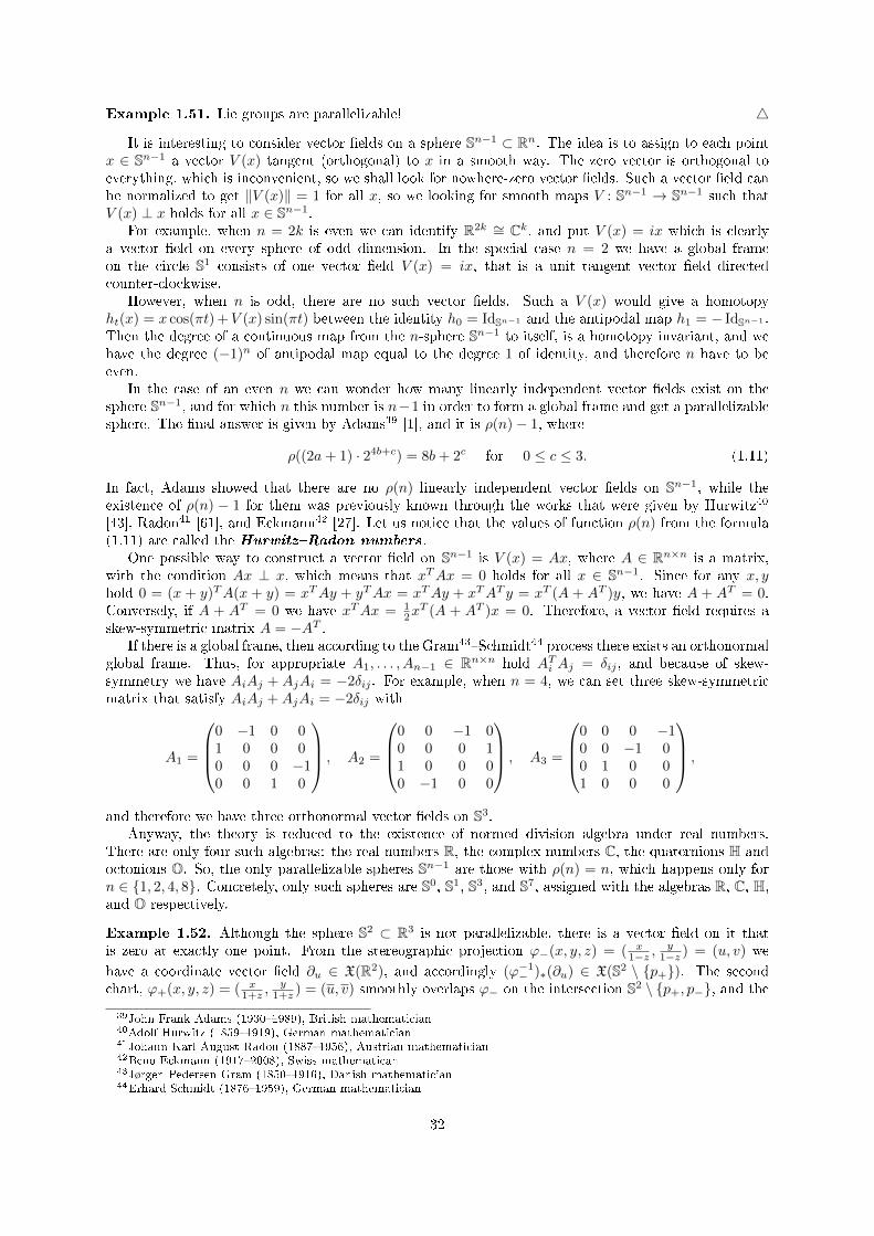
Example 1.51. Lie groups are parallelizable! 4

It is interesting to consider vector elds on a sphere Sn−1 ⊂ Rn. The idea is to assign to each pointx ∈ Sn−1 a vector V (x) tangent (orthogonal) to x in a smooth way. The zero vector is orthogonal toeverything, which is inconvenient, so we shall look for nowhere-zero vector elds. Such a vector eld canbe normalized to get ‖V (x)‖ = 1 for all x, so we looking for smooth maps V : Sn−1 → Sn−1 such thatV (x) ⊥ x holds for all x ∈ Sn−1.

For example, when n = 2k is even we can identify R2k ∼= Ck, and put V (x) = ix which is clearlya vector eld on every sphere of odd dimension. In the special case n = 2 we have a global frameon the circle S1 consists of one vector eld V (x) = ix, that is a unit tangent vector eld directedcounter-clockwise.

However, when n is odd, there are no such vector elds. Such a V (x) would give a homotopyht(x) = x cos(πt) +V (x) sin(πt) between the identity h0 = IdSn−1 and the antipodal map h1 = − IdSn−1 .Then the degree of a continuous map from the n-sphere Sn−1 to itself, is a homotopy invariant, and wehave the degree (−1)n of antipodal map equal to the degree 1 of identity, and therefore n have to beeven.

In the case of an even n we can wonder how many linearly independent vector elds exist on thesphere Sn−1, and for which n this number is n−1 in order to form a global frame and get a parallelizablesphere. The nal answer is given by Adams39 [1], and it is ρ(n)− 1, where

ρ((2a+ 1) · 24b+c) = 8b+ 2c for 0 ≤ c ≤ 3. (1.11)

In fact, Adams showed that there are no ρ(n) linearly independent vector elds on Sn−1, while theexistence of ρ(n) − 1 for them was previously known through the works that were given by Hurwitz40

[43], Radon41 [61], and Eckmann42 [27]. Let us notice that the values of function ρ(n) from the formula(1.11) are called the HurwitzRadon numbers.

One possible way to construct a vector eld on Sn−1 is V (x) = Ax, where A ∈ Rn×n is a matrix,with the condition Ax ⊥ x, which means that xTAx = 0 holds for all x ∈ Sn−1. Since for any x, yhold 0 = (x + y)TA(x + y) = xTAy + yTAx = xTAy + xTAT y = xT (A + AT )y, we have A + AT = 0.Conversely, if A + AT = 0 we have xTAx = 1

2xT (A + AT )x = 0. Therefore, a vector eld requires a

skew-symmetric matrix A = −AT .If there is a global frame, then according to the Gram43Schmidt44 process there exists an orthonormal

global frame. Thus, for appropriate A1, . . . , An−1 ∈ Rn×n hold ATi Aj = δij , and because of skew-symmetry we have AiAj + AjAi = −2δij . For example, when n = 4, we can set three skew-symmetricmatrix that satisfy AiAj +AjAi = −2δij with

A1 =

0 −1 0 01 0 0 00 0 0 −10 0 1 0

, A2 =

0 0 −1 00 0 0 11 0 0 00 −1 0 0

, A3 =

0 0 0 −10 0 −1 00 1 0 01 0 0 0

,

and therefore we have three orthonormal vector elds on S3.Anyway, the theory is reduced to the existence of normed division algebra under real numbers.

There are only four such algebras: the real numbers R, the complex numbers C, the quaternions H andoctonions O. So, the only parallelizable spheres Sn−1 are those with ρ(n) = n, which happens only forn ∈ 1, 2, 4, 8. Concretely, only such spheres are S0, S1, S3, and S7, assigned with the algebras R, C, H,and O respectively.

Example 1.52. Although the sphere S2 ⊂ R3 is not parallelizable, there is a vector eld on it thatis zero at exactly one point. From the stereographic projection ϕ−(x, y, z) = ( x

1−z ,y

1−z ) = (u, v) we

have a coordinate vector eld ∂u ∈ X(R2), and accordingly (ϕ−1− )∗(∂u) ∈ X(S2 \ p+). The second

chart, ϕ+(x, y, z) = ( x1+z ,

y1+z ) = (u, v) smoothly overlaps ϕ− on the intersection S2 \ p+, p−, and the

39John Frank Adams (19301989), British mathematician40Adolf Hurwitz (18591919), German mathematician41Johann Karl August Radon (18871956), Austrian mathematician42Beno Eckmann (19172008), Swiss mathematican43Jørgen Pedersen Gram (18501916), Danish mathematician44Erhard Schmidt (18761959), German mathematician

32

relations are (u, v) = ϕ− ϕ−1+ (u, v) = ( u

u2+v2, vu2+v2

) and (u, v) = ϕ+ ϕ−1− (u, v) = ( u

u2+v2 ,v

u2+v2 ).Then

∂u = ∂u(u)∂u + ∂u(v)∂v =v2 − u2

(u2 + v2)2∂u +

−2uv

(u2 + v2)2∂v = (v2 − u2)∂u − 2uv∂v,

so (ϕ−1− )∗(∂u) can be extended to the point p+. Concretely, we have the formula

Vt =

((ϕ−1− )∗(∂u))t for t ∈ S2 \ p+

((ϕ−1+ )∗

((v2 − u2)∂u − 2uv∂v

))tfor t ∈ S2 \ p−

which denes V at every point of the sphere S2. Since it is smooth in local coordinates, V ∈ X(S2)obviously holds. Of course, Vp+ = 0, while Vt = ((ϕ−1

− )∗(∂u))t 6= 0 on S2 \ p+. 4

1.15 Covector elds

The cotangent space of a manifold M at a point p ∈M is the dual space of the tangent space,

T ∗pM = (TpM)∗ = hom(TpM,R).

Elements of the cotangent space T ∗pM are covectors at p, which means linear functions ωp : TpM → R.Following the theory of vector elds, we want to investigate a map ω that smoothly assigns to each pointp ∈M a covector ωp at p.

For example, for every function f ∈ F(M) we dene its dierential df , that assigns to each pointp ∈ M a covector dfp ∈ T ∗pM given by dfp(Xp) = Xp(f) for Xp ∈ TpM . Example 1.33 shows a tangent

map for f ∈ F(M) with Tpf(Xp) = Xp(f)( ddt )p. Therefore, if we take advantage of the identicationTf(p)R ∼= R, then we can naturally identify dfp with Tpf .

Let us set a chart (U,ϕ) at a point p ∈ M and its coordinate functions xi = πi ϕ. By Theorem1.24, ( ∂

∂x1)p, . . . , (

∂∂xn

)p form a basis of the tangent space TpM . Since (dxi)p(∂∂xj

)p = ( ∂∂xj

)p(xi) = δijfor 1 ≤ i, j ≤ n, covectors (dx1)p, . . . , (dxn)p form a basis of the cotangent space T ∗pM that is dual togiven basis for TpM . Additionally, for ωp ∈ T ∗pM and Xp ∈ TpM , from Theorem 1.24 follows

ωp(Xp) = ωp

(n∑i=1

Xp(xi)

(∂

∂xi

)p

)=

n∑i=1

Xp(xi)ωp

((∂

∂xi

)p

)=

n∑i=1

ωp

((∂

∂xi

)p

)(dxi)p(Xp),

and hence ωp =∑ni=1 ωp((∂i)p) (dxi)p.

Theorem 1.43. Let Mn be a manifold, and (U,ϕ) is a chart at p ∈M with xi = πi ϕ. Then covectors(dx1)p, . . . , (dxn)p form a basis for T ∗pM and ωp =

∑ni=1 ωp((∂i)p) (dxi)p holds for all ωp ∈ T ∗pM .

Since we want a map ω : p 7→ ωp to be smooth, it is necessary that the codomain is some manifold.Following the tangent bundle, we will make the cotangent bundle T ∗M =

⊔p∈M T ∗pM of a manifoldM

as a union of all cotangent spaces. As before, it goes in a package with a natural projection π : T ∗M →Mwhich is given with π(ωp) = p for ωp ∈ T ∗pM . We can imitate the tangent bundle construction and givea topology to the set T ∗M .

Let (U,ϕ) be a chart on M with coordinate functions xi = πi ϕ. A covector ωp ∈ T ∗pM at a pointp ∈ U is by Theorem 1.43 a unique linear combination ωp =

∑ni=1 ωp((∂i)p) (dxi)p, that motivate us to

set up a map ϕ : T ∗U → ϕ(U)× Rn ⊆ R2n with

ϕ(ωp) =

(x1(p), . . . , xn(p), ωp

(∂

∂x1

)p

, . . . , ωp

(∂

∂xn

)p

).

A map ϕ is a bijection with the inverse ϕ−1(ϕ(p), λ1, . . . , λn) =∑ni=1 λi (dxi)p, which helps to transfer

the topology from ϕ(U)× Rn to T ∗U . We can obtain the topology basis by picking up all open subsetsof T ∗U for any coordinate neighbourhood U from the complete smooth atlas.

33

Let us examine compatibility of charts (T ∗U, ϕ) and (T ∗V, ψ) on T ∗M , where (U,ϕ) and (V, ψ) are

charts on M . From the coordinate change (1.7) we have ( ∂∂yk

)p =∑nj=1

∂xj∂yk

(p)( ∂∂xj

)p, and therefore

(dxi)p(∂∂yk

)p = ∂xi∂yk

(p), so we calculate the transition map with

(ψ ϕ−1)(ϕ(p), λ1, . . . , λn) = ψ

(n∑i=1

λi (dxi)p

)

=

(ψ(p),

n∑i=1

λi (dxi)p

(∂

∂x1

)p

, . . . ,

n∑i=1

λi (dxi)p

(∂

∂xn

)p

)

=

(ψ(p),

n∑i=1

λi∂(πi (ϕ ψ−1))

∂π1(ψ(p)), . . . ,

n∑i=1

λi∂(πi (ϕ ψ−1))

∂πn(ψ(p))

),

that is smooth because of ψ(p) = (ψ ϕ−1)(ϕ(p)). After remaining technical details left for the exercise,it turns out that T ∗M is a smooth manifold of dimension 2n.

Consider sections of the cotangent bundle, which are maps ω : M → T ∗M such that π ω = IdM .The covector eld is a smooth section of the cotangent bundle T ∗M , and the set of all covector eldswe shall denote with X∗(M). If (U,ϕ) is a chart on M with coordinate functions xi = πi ϕ, then everysection ω of the cotangent bundle T ∗U can be written as a linear combination ω =

∑ni=1 ai dxi, where

coecients ai : U → R are some functions. Smoothness of these coecients depends of smoothness ofsections.

Lemma 1.44. If (U,ϕ) is a chart on M with coordinate functions xi = πi ϕ, then a section ω =∑ni=1 ai dxi of the cotangent bundle T

∗U is smooth if and only if all coecient functions ai : U → R aresmooth.

Proof. From Theorem 1.43 follows that ai(p) = ωp(∂∂xi

)p. For an appropriate chart (T ∗U, ϕ) we haveϕ = (ϕ, a1, . . . , an) π, which means ϕ ω = (ϕ, a1, . . . , an). Since ϕ is a dieomorphism, ω is smooth ifand only if all functions ai are smooth.

For example, for f ∈ F(M), we can consider the dierential df that in every chart (U,ϕ) have a formdf =

∑ni=1 ai dxi. Acting on coordinate vectors we get coecients,

∂f

∂xj=

(∂

∂xj

)f = (df)

(∂

∂xj

)=

n∑i=1

ai dxi

(∂

∂xj

)=

n∑i=1

aiδij = aj ,

that are obviously smooth, so we have a covector eld df ∈ X∗(M), and a local expression:

df =

n∑i=1

∂f

∂xidxi. (1.12)

Example 1.53. The dierential of a function f : R2 → R given by f(x, y) = xy2 sinx is

df =∂(xy2 sinx)

∂xdx+

∂(xy2 sinx)

∂ydy = (y2 sinx+ xy2 cosx) dx+ (2xy sinx) dy.

4

We can be directly assured that the dierential has the following nice properties. First, the dierentiald : F(M) → X∗(M) is an R-linear map. For f, h ∈ F(M) holds d(fh) = hdf + fdh. For f ∈ F(M) andh ∈ F(R) holds d(h f) = (h′ f)df . Of course, for constant f ∈ F(M) we have df = 0, while by Lemma1.39 we have that df = 0 for a connected M implies constant f .

For every section ω of the cotangent bundle T ∗M and an arbitrary vector eld X ∈ X(M), we cannaturally dene a function ω(X) : M → R with ω(X)p = ωp(Xp) for p ∈ M . For an arbitrary functionf : M → R we have ω(fX)p = ωp(f(p)Xp) = f(p)ωp(Xp) = (fω(X))p from where follows linearity forfunctions, ω(fX) = fω(X). A covector eld ω ∈ X∗(M) is a smooth section ω : M → T ∗M , but also amap ω : X(M)→ F(M), depending on what suits us more.

34

Lemma 1.45. A section ω of the cotangent bundle T ∗M is smooth if and only if for every X ∈ X(M)holds ω(X) ∈ F(M).

Proof. For an arbitrary section ω : M → T ∗M in some chart (U,ϕ) on M , by Theorem 1.43 we haveω =

∑ni=1 ω(∂i) dxi. Since X =

∑nj=1X(xj)∂j holds from Theorem 1.24, we can calculate ω(X) =∑n

i,j=1 ω(∂i)X(xj) dxi(∂j) =∑ni=1 ω(∂i)X(xi). So, it is obvious that a smooth section ω gives a smooth

ω(X) on an arbitrary coordinate neighbourhood of a manifold M , so smooth on the whole M , andtherefore ω(X) ∈ F(M). Conversely, if ω(X) ∈ F(M) holds for all X ∈ X(M), it especially holds for ∂i,so ω =

∑ni=1 ω(∂i) dxi has smooth coecients and by Lemma 1.44, ω is smooth.

Let f : M → N be a smooth map between manifolds. The global tangent map f∗ = Tf : TM → TNpushes tangent vector forward from M to N . Dualizing this leads to a map on covectors going in theopposite direction, from N to M . The pullback is a map f∗ : T ∗N → T ∗M dened by

(f∗(ωf(p)))(Xp) = ωf(p)(f∗(Xp))

for a covector ωf(p) ∈ T ∗f(p)N and a vector Xp ∈ TpM .Unlike vector elds which in general can not be pushed by smooth map, covector elds always pull back

to covector elds. For a covector eld ω ∈ X(N) we dene the pullback f∗ω as a section of the cotangentbundle T ∗M such that (f∗ω)p = f∗(ωf(p)) holds for p ∈ M , witch means (f∗ω)p(Xp) = ωf(p)(f∗(Xp))for all Xp ∈ TpM .

Let f : M → N be smooth, p ∈M , and Xp ∈ TpM . Functions h ∈ F(N) also have the pullback givenby f∗h = h f ∈ F(M). From (f∗dh)p(Xp) = (dh)f(p)(f∗(Xp)) = (f∗(Xp))h = Xp(h f) = Xp(f

∗h) =(df∗h)p(Xp) follows that the pullback and the dierential commutes, f∗(dh) = d(f∗h). It can also beeasily proved that for covector elds ω, τ ∈ X∗(N) hold f∗(ω+τ) = f∗ω+f∗τ , and f∗(hω) = (f∗h)(f∗ω)where h ∈ F(M).

Theorem 1.46. If f : M → N is smooth and ω ∈ X∗(N) then f∗ω ∈ X∗(M).

Proof. For p ∈ M we can choose a chart (U,ϕ) at p ∈ M with xj = πj ϕ for 1 ≤ j ≤ m = dimMand a chart (V, ψ) at f(p) ∈ N with yi = πi ψ for 1 ≤ i ≤ n = dimN such that f(U) ⊆ V . SinceωV =

∑ni=1 ai dyi holds for some ai ∈ F(V ), from (1.12) we have

(f∗ω)U=

n∑i=1

(f∗ai)f∗(dyi) =

n∑i=1

(f∗ai) df∗yi =

n∑i=1

(ai f) d(yi f) =

n∑i=1

m∑j=1

(ai f)∂(yi f)

∂xjdxj .

Since coecients∑ni=1(ai f)∂(yif)

∂xjare smooth, by Lemma 1.44, f∗ω is smooth on U , and also smooth

at a point p for each p ∈M , so f∗ω ∈ X∗(M).

Example 1.54. Let f : R3 → R2 is given by (u, v) = f(x, y, z) = (x2y, y sin z) and let ω ∈ X∗(R2) isgiven by ω = u dv + v du. We can calculate f∗ω with

f∗ω = (f∗u)(f∗dv) + (f∗v)(f∗du) = (u f) d(v f) + (v f) d(u f)

= (x2y) d(y sin z) + (y sin z) d(x2y) = x2y(sin z dy + y cos z dz) + (y sin z)(2xy dx+ x2 dy)

= 2xy2 sin z dx+ 2x2y sin z dy + x2y2 cos z dz.

4

1.16 Tensor elds

The notion of tensor eld on a manifoldM generalizes the notions of smooth real-valued functions F(M),vector elds X(M), and covector elds X∗(M), and therefore provides more complicated objects on amanifold. Tensors occur in many dierent guises, but their common characteristic is multilinearity.

In some general case we can consider a module V over ring K, and its dual module V∗ = hom(V,K).A tensor of type (r, s) ∈ N0 × N0 over V is a K-multilinear function A : (V∗)r × (V)s → K. The setTrs(V) of all tensors of type (r, s) over V is a module over K with usual denitions of addition and scalarmultiplication.

35

A tensor eld A on a manifold M is a tensor over the F(M)-module X(M). It actually means thata F(M)-multilinear function

A : X∗(M)× · · · × X∗(M)︸ ︷︷ ︸r

×X(M)× · · · × X(M)︸ ︷︷ ︸s

→ F(M),

is a tensor eld of type (r, s) ∈ N0 ×N0. Thus, the set Trs(M) of all tensor elds on M of type (r, s) is a

module over F(M).

Example 1.55. A tensor eld generalizes the previously introduced notions. For example, in the specialcase (r, s) = (0, 0), tensor leds are simply smooth functions on M , T0

0(M) = F(M). Covector eldsω ∈ X∗(M) are by Lemma 1.45 F(M)-linear maps ω : X(M) → F(M) so T0

1(M) = X∗(M). Finally,each X ∈ X(M) determines a tensor eld A : X∗(M) → F(M) with A(ω) = ω(X), while the converse isX(f) = df(X) = A(df) for f ∈ F(M), and therefore we have the identication T1

0(M) = X(M). 4

To prove that a given function A : X∗(M)r × X(M)s → F(M) is a tensor, we have ti show that it isF(M)-linear in each slot (in each variable separately). Additivity in each slot is often obvious, so themain question is whether functions from F(M) can be factored out A of each slot:

A(ω1, . . . , ωr, X1, . . . , fXi, . . . , Xs) = fA(ω1, . . . , ωr, X1, . . . , Xi, . . . , Xs)

Example 1.56. Consider a function E : X∗(M) × X(M) → F(M) given by E(ω,X) = ω(X). It isobviously F(M)-linear in both slots, so E ∈ T1

1(M). 4

Example 1.57. For a non-zero covector eld ω ∈ X∗(M) we can dene F : X(M)× X(M)→ F(M) byF (X,Y ) = X(ω(Y )). The function F is F(M)-linear in the rst slot, but in the second slot it is onlyadditive, because of F (X, fY ) = X(ω(fY )) = X(fω(Y )) = (Xf)ω(Y ) + fF (X,Y ), so F is not a tensoreld. 4

Example 1.58. Every F(M)-multilinear map A : X(M)s → X(M) can be naturally identied withA : X∗(M)×X(M)s → F(M), A(ω,X1, . . . , Xs) = ω(A(X1, . . . , Xs)), so we have the induced tensor eldA ∈ T1

s(M). 4

Tensors of type (0, s) are said to be covariant of order s, while tensors of type (r, 0) are said tobe contravariant of order r ≥ 1. For example, real-valued functions and covector elds are covarianttensors, while vector elds are contravariant tensors.

While we can add only tensors of the same type, any two tensors can be multiplied. For A1 ∈ Tr1s1(M)and A2 ∈ Tr2s2(M) we dene A1 ⊗A2 : X∗(M)r1+r2 × X(M)s1+s2 → F(M) with

(A1 ⊗A2)(ω1, . . . , ωr1+r2 , X1, . . . , Xs1+s2)

= A1(ω1, . . . , ωr1 , X1, . . . , Xs1)A2(ωr1+1, . . . , ωr1+r2 , Xs1+1, . . . , Xs1+s2).

Then A1 ⊗A2 is a tensor of type (r1 + r2, s1 + s2) called the tensor product of A1 and A2. Especially,for A ∈ Trs(M) and f ∈ F(M) we have A ⊗ f = f ⊗ A = fA, while additional A ∈ F(M) gives theordinary multiplication of functions in F(M).

The tensor product is F(M)-linear, so (f1A1 + f2A2)⊗B = f1A1 ⊗B + f2A2 ⊗B holds for f1, f2 ∈F(M), A1, A2 ∈ Tr1s1(M), B ∈ Tr2s2(M). Also, directly from the denition we have that the tensor productis associative, so for tensors A,B,C of any types we often write without brackets A ⊗ B ⊗ C. We cannotice that for a covariant tensor A and a contravariant tensor B by denition holds A ⊗ B = B ⊗ A.However, although functions commute with anything, f(A ⊗ B) = (fA) ⊗ B = A ⊗ (fB), the tensorproduct in general is not commutative.

Example 1.59. On a coordinate neighbourhood we have (dx1⊗dx2)(∂1, ∂2) = dx1(∂1) dx2(∂2) = 1 and(dx2 ⊗ dx1)(∂1, ∂2) = dx2(∂1) dx1(∂2) = 0, so dx1 ⊗ dx2 6= dx2 ⊗ dx1. 4

Just as for a vector eld or a covector eld, any tensor eld A on a manifold M can be viewed asa eld, assigning a value Ap at each point p ∈ M . It turns out that the value Ap does not depend onwhole vector and covector elds, not even from their values in some neighbourhood of p, but solely fromtheir individual values at the point p.

36

Lemma 1.47. If any one of covector elds ω1, . . . , ωr or vector elds X1, . . . , Xs vanishes at p ∈ M ,then A(ω1, . . . , ωr, X1, . . . , Xs)(p) = 0 holds for A ∈ Trs(M).

Proof. Let (U,ϕ) be a chart at p ∈ M with xi = πi ϕ ∈ F(U). By Lemma 1.17 there is a bumpfunction b ∈ F(M) supported in U that is 1 on some open neighbourhood of p, which allows extensionsbXj(xi) ∈ F(M) and b∂i ∈ X(M). Therefore we have

b2A(. . . , Xj , . . . ) = A(. . . , b2Xj , . . . ) = A(. . . ,

n∑i=1

bXj(xi) b∂i, . . . ) =

n∑i=1

bXj(xi)A(. . . , b∂i, . . . ),

b2A(. . . , ωj , . . . ) = A(. . . , b2ωj , . . . ) = A(. . . ,

n∑i=1

bωj(∂i) b dxi, . . . ) =

n∑i=1

bωj(∂i)A(. . . , b dxi, . . . ).

If (Xj)p = 0 for some 1 ≤ j ≤ s, we have (bXj(xi))(p) = 0, hence A(. . . , Xj , . . . )(p) = 0. Similarly,(ωj)p = 0 for some 1 ≤ j ≤ r implies (bωj(∂i))(p) = 0, thus A(. . . , ωj , . . . )(p) = 0.

Theorem 1.48. Let A ∈ Trs(M) and p ∈ M such that for ωi, ωi ∈ X∗(M) and Xj , Xj ∈ X(M) hold(ωi)p = (ωi)p and (Xj)p = (Xj)p where 1 ≤ i ≤ r and 1 ≤ j ≤ s. Then A(ω1, . . . , ωr, X1, . . . , Xs)(p) =A(ω1, . . . , ωr, X1, . . . , Xs)(p).

Proof. Let us notice that the dierence of tensorsA(ω1, . . . , ωr, X1, . . . , Xs)−A(ω1, . . . , ωr, X1, . . . , Xs) =A(ω1−ω1, . . . , ωr, X1, . . . , Xs)+A(ω1, ω2−ω2 . . . , ωr, X1, . . . , Xs)+· · ·+A(ω1, . . . , ωr, X1, . . . , Xs−Xs),is equal to zero, since by Lemma 1.47 all r + s terms vanish at the point p.

Directly from Theorem 1.48 follows that a tensor eld A ∈ Trs(M) has a value Ap at each pointp ∈M , which is a funciton Ap : (T ∗pM)r × (TpM)s → R given by

Ap((ω1)p, . . . , (ωr)p, (X1)p, . . . , (Xs)p) = A(ω1, . . . , ωr, X1, . . . , Xs)(p).

It is easy to check R-multilinearity of the function Ap, so by restriction of tensor eld A ∈ Trs(M) atp ∈M we get a tensor Ap ∈ Trs(TpM). Just as a vector eld is a smooth section of the tangent bundle,a tensor eld A ∈ Trs(M) can be considered as a smooth section of the appropriate tensor bundle thatassigns to each point p ∈ M a tensor Ap. Especially, this interpretation allows that the restriction AUof a tensor eld A ∈ Trs(M) to an open subest U ⊂ M can be seen as a well dened tensor eld on U ,i.e. AU∈ Trs(U).

Let (U,ϕ) be a chart on a manifold Mn, and xi = πi ϕ are its coordinate functions. Coordinateformulas, X =

∑iX(xi)∂i for vector elds and ω =

∑i ω(∂i) dxi for covector elds, can be extended to

tensor elds of arbitrary type. Components of a tensor eld A ∈ Trs(M) are functions

Ai1...irj1...js= A

(dxi1 , . . . , dxir ,

∂

∂xj1, . . . ,

∂

∂xjs

)∈ F(U),

for all indices 1 ≤ i1, . . . , ir, j1, . . . , js ≤ n.For ω ∈ T0

1(M) = X∗(M) the components are ωi = ω(∂i), as can be seen in the formula ω =∑i ωi dxi.

Similarly, for X ∈ T10(M) = X(M), the components are Xi = X(dxi) = dxi(X) = X(xi), as can be seen

in the formula X =∑iX

i∂i.If a (1, s) tensor eld is given by A : X(M)s → X(M), its components are determined directly

through the equation A(∂i1 , . . . , ∂is) =∑j A

ji1...is

∂j , because for its interpretation A ∈ T1s(M) we have

A(dxj , ∂i1 , . . . , ∂is) = dxj(A(∂i1 , . . . , ∂is)) =∑k A

ki1...is

dxj(∂k) = Aji1...is .Generally, a tensor eld A ∈ Trs(M) can be expressed by its components with

A(ω1, . . . , ωr, X1, . . . , Xs) =∑

1≤i1,...,ir,j1,...,js≤n

Ai1...irj1...js(ω1)i1 · · · (ωr)ir (X1)j1 · · · (Xs)

js .

In a xed chart, components of a sum of tensors are just the sum of the components. On the other hand,the components of a tensor product are given by

(A⊗B)i1...ir+r′j1...js+s′

= Ai1...irj1...js·Bir+1...ir+r′

js+1...js+s′,

37

and thereforeA =

∑1≤i1,...,ir,j1,...,js≤n

Ai1...irj1...js∂i1 ⊗ · · · ⊗ ∂ir ⊗ dxj1 ⊗ · · · ⊗ dxjs .

There is an interesting operation on the set of tensors called contraction that tensors of type (r, s)shrink to tensor of type (r − 1, s− 1). The general denition is based on the following special case.

Lemma 1.49. There is a unique F(M)-linear function C : T11(M)→ F(M) such that C(X ⊗ω) = ω(X)

for all X ∈ X(M) and ω ∈ X∗(M).

Proof. In a coordinate neighbourhood U , A ∈ T11(M) can be expressed by A =

∑ni,j=1A

ij ∂i⊗dxj . Since

it must be C(∂i ⊗ dxj) = dxj(∂i) = δij , we have to dene C(A) =∑ni=1A

ii =

∑ni=1A(dxi, ∂i). Such C

has the required properties on U . To extend the function on the whole manifold it suces to show thatthis denition is independent of the choice of coordinate system,

∑k

A

(dyk,

∂

∂yk

)=∑k

A

∑i

∂yk∂xi

dxi,∑j

∂xj∂yk

∂

∂xj

=∑i,j,k

∂yk∂xi

∂xj∂yk

A

(dxi,

∂

∂xj

)

=∑i,j

δijA

(dxi,

∂

∂xj

)=∑i

A

(dxi,

∂

∂xi

).

The function C from the previous lemma is called (1, 1) contraction . In general, we can chooseone contravariant slot 1 ≤ i ≤ r and one covariant slot 1 ≤ j ≤ s, and apply C to the function(ωi, Xj) 7→ A(ω1, . . . , ωr, X1, . . . , Xs) that for xed ω1, . . . ωi−1, ωi+1, . . . , ωr, X1 . . . Xj−1, Xj+1, . . . , Xs

is a (1, 1) tensor. The new function (Cij)(ω1, . . . ωi−1, ωi+1, . . . , ωr, X1 . . . Xj−1, Xj+1, . . . , Xs) ∈ F(M),

is evidently F(M)-multilinear, thus Cij ∈ Tr−1s−1(M) and we call it the contraction of A over i, j. The

components of the contraction are

(CijA)i1...ir−1

j1...js−1=

n∑k=1

Ai1...ii−1 k ii...ir−1

j1...jj−1 k jj ...js−1.

The pullback of a covariant eld can be generalized to the pullback of a covariant tensor. Letf : M → N be a smooth map between manifolds. The pullback of a covariant tensor A ∈ T0

s(N) isdened by (f∗A)(X1, . . . , Xs) = A(f∗(X1), . . . , f∗(Xs)) for all p ∈ M , Xi ∈ TpM . At any point p ∈ M ,the pullback f∗(A) gives a R-multilinear function from (TpM)s to R, which is a (0, s) tensor over TpM .Coordinate computations show that f∗(A) is a covariant tensor eld on M .

Thus, for a smooth f : M → N and each s ≥ 0 we have R-linear f∗ : T0s(N)→ T0

s(M). Additionally,for A ∈ T0

s(N) and B ∈ T0t (N) we have f∗(A ⊗ B) = f∗(A) ⊗ f∗(B). Also, for a smooth h : N → P

holds (h f)∗ = f∗ h∗ : T0s(P )→ T0

s(M).For a covariant or contravariant tensor of order at least 2 we say that is symmetric if transposing

any two of its arguments we get the same value. If each such transposition produces a sign change thenwe say that this tensor is skew-symmetric.

1.17 Tensor derivations

In the previous section we have seen the algebraic side of the tensor elds, and now we shall consider sometensor calculus. A tensor derivation on a manifoldM is a set of R-linear functions ∇ = ∇rs : Trs(M)→Trs(M) for (r, s) ∈ N0×N0 such that for any tensor eldsA,B ∈ Trs(M) hold∇(A⊗B) = ∇A⊗B+A⊗∇B,and also ∇(CA) = C(∇A) for any contraction C.

Thus, the derivative ∇ is R-linear, preserves tensor type, obeys Leibniz rule, and commutes with allcontractions. For f ∈ F(M) holds fA = f ⊗A, so we have ∇(fA) = (∇f)A+ f∇A. Especially, ∇0

0 is aderivation on T0

0(M) = F(M), so there is a unique vector eld X ∈ X(M) such that ∇f = Xf holds forall f ∈ F(M).

Since a tensor derivation is not F(M)-linear, in general the value of ∇A at a point p ∈ M cannotusually be found from Ap only. However, it can be found from the values od A on any arbitrarily smallneighbourhood of p. This local character of tensor derivation can be expressed as follows.

38

Theorem 1.50. if ∇ is a tensor derivative on a manifold M and U ⊂M is an open subset, then thereexists a unique tensor derivation ∇U on U such that ∇U (AU ) = (∇A)U holds for all tensor elds onM .

Proof. For an arbitrary p ∈ U we can choose a bum function b supported in U and equal to 1 on someneighbourhood of p. For A ∈ Trs(U) holds bA ∈ Trs(M) and we dene (∇UA)p = (∇(bA))p. It can beshown that this denition does not depend of the choice of bump function, and ∇UA ∈ Trs(U) holds.Then we can show that ∇U is a tensor derivative on U and has the stated restriction properties, andalso that it is unique.

The Leibnizian formula ∇(A ⊗ B) = ∇A ⊗ B + A ⊗ ∇B can be reformed and generalized in thefollowing way.

Theorem 1.51. For a tensor derivation ∇ on M and A ∈ Trs(M) we have

∇(A(ω1, . . . ,ωr, X1, . . . , Xs)

)= (∇A)(ω1, . . . , ωr, X1, . . . , Xs)

+

r∑i=1

A(ω1, . . . ,∇ωi, . . . ωr, X1, . . . , Xs) +

s∑j=1

A(ω1, . . . ωr, X1, . . . ,∇Xj , . . . , Xs).

Proof. Since A(ω1, . . . , Xs) =∑i1,...,js

Ai1...irj1...js(ω1)i1 . . . (ωr)ir (X1)j1 . . . (Xs)

js , and A⊗ω1⊗· · ·⊗Xs has

components Ai1...irj1...js(ω1)k1 . . . (ωr)kr (X1)l1 . . . (Xs)

ls , we have r + s contractions for

A(ω1, . . . , Xs) = Ci1k1 . . . CirkrCl1j1 . . . C

lsjs

(A⊗ ω1 ⊗ · · · ⊗Xs),

so it is not hard to conclude that the theorem holds.

From Theorem 1.51 we see that the term involving ∇A can be expressed in terms of ∇ applied solelyto functions, vector elds, and covector elds. Moreover, since ω ∈ X∗(M) holds we have (∇ω)(X) =∇(ωX)− ω(∇X), it is enough to know only derivatives of functions and vector elds. It turns out thatthe converse is also true, which means that from suitable data on F(M) and X(M) we can construct atensor derivation.

Theorem 1.52. For a vector eld ∇00 : F(M) → F(M) and an R-linear map ∇1

0 : X(M) → X(M) suchthat ∇1

0(fX) = (∇00f)X + f∇1

0X holds for all f ∈ F(M) and X ∈ X(M), there is a unique tensorderivation ∇ on M whose ∇0

0 and ∇10 are appropriate parts.

Proof. Uniqueness follows from Theorem 1.51 which we shall also use to complete ∇. First, for ω ∈X∗(M) we have to dene (∇0

1ω)(X) = ∇00(ω(X))− ω(∇1

0X), so

(∇01ω)(fX) = ∇0

0(ω(fX))− ω(∇10fX) = ∇0

0(fω(X))− ω((∇00f)X + f∇1

0X)

= (∇00f)ω(X) + f∇0

0(ω(X))− (∇00f)ω(X)− fω(∇1

0X) = f(∇01ω)(X),

which means that∇01ω is F(M)-linear and therefore∇0

1ω ∈ X∗(M). It is also easy to see that∇01 : X∗(M)→

X∗(M) is R-linear. By Theorem 1.51, ∇rsA for r + s ≥ 2 and A ∈ Trs(M) must be

(∇rsA)(ω1, . . . ,ωr, X1, . . . , Xs) = ∇00

(A(ω1, . . . , ωr, X1, . . . , Xs)

)−

r∑i=1

A(ω1, . . . ,∇01ωi, . . . ωr, X1, . . . , Xs)−

s∑j=1

A(ω1, . . . ωr, X1, . . . ,∇10Xj , . . . , Xs),

so we dene it in this way. As before, we should check that ∇rsA is F(M)-multilinear, i.e. ∇rsA ∈ Trs(M),and also that ∇rs : Trs(M)→ Trs(M) is R-linear. The next step is a direct computation which shows thatholds ∇(A⊗B) = ∇A⊗B +A⊗∇B.

It remains to prove that a tensor derivative commutes with contractions. For example, for C : T11(M)→

F(M) we have ∇C(ω ⊗X) = ∇(ω(X)) = (∇ω)(X) + ω(∇X) = C(∇ω ⊗X + ω ⊗∇X) = C∇(ω ⊗X),where we see that C and ∇ commute on tensors of form ω⊗X. Locality of ∇ allows calculations on co-ordinate neighbourhoods, where we know that all tensor elds of type (1, 1) are sums of tensor products.At the end this process we should extend to all contractions.

39

Example 1.60. For any V ∈ X(M), by the previous theorem, we can set a tensor derivative LV on Mby LV (f) = V f for all f ∈ F(M) and by LV (X) = [V,X] for all X ∈ X(M). The conditions of thetheorem are satised since (LV )0

0 = V is a vector eld, (LV )10 = [V, ·] is R-linear, and we also have the

equation LV (fX) = [V, fX] = (V f)X + f [V,X] = (LV f)X + fLVX. This tensor derivative LV we callthe Lie derivative relative to V . 4

40

Chapter 2

Pseudo-Riemannian geometry

This chapter is an introduction to a pseudo-Riemannian geometry. An excellent reference for the classicaltreatment of pseudo-Riemannian geometry is the book by O'Neill [59]. We also recommend Lee [46].Some standard texts for Riemannian geometry are given by Lee [48] and do Carmo1 [18]. We insist onthe indenite case, so we nd valuable texts by Meinrenken2 [49] and Clark3 [23].

2.1 Scalar products

Let V be a nite-dimensional vector space over R. A bilinear form on V is an R-bilinear functiong : V × V → R. A bilinear form g is called symmetric if it satises g(X,Y ) = g(Y,X) for all X,Y ∈ V.A symmetric bilinear form g is uniquely determined by the associated quadratic form ε : V → R givenby εX = g(X,X). Namely, we recover g from ε using the polarization identity

g(X,Y ) =1

2(εX+Y − εX − εY ). (2.1)

We say that a symmetric bilinear form g is nondegenerate if g(X,Y ) = 0 for all Y ∈ V impliesX = 0. Additionally, if for all X 6= 0 holds g(X,X) > 0 then g is positive denite . Similarly, if for allX 6= 0 holds g(X,X) < 0 then g is negative denite . If g is positive denite or negative denite wesay that g is denite , otherwise it is indenite . Evidently, if g is denite, then it is nondegenerate.

A scalar product g is a nondegenerate symmetric bilinear form on V. A nite-dimensional realvector space V together with a scalar product g will be referred to as a scalar product space (or aquadratic space) (V, g).

Each bilinear form g on V, in the presence of an ordered basis (E1, . . . , En) in V, has the associatedGram matrix G with entries gij = g(Ei, Ej). It recovers g by g(

∑ni=1 αiEi,

∑nj=1 βjEj) =

∑ni,j=1 αiβjgij ,

and g is symmetric if and only if G is symmetric. Moreover, a scalar product has invertible Gram matrix.

Lemma 2.1. A symmetric bilinear form g on a nite-dimensional real vector space V is nondegenerateif and only if its Gram matrix with respect to any basis of V has nonzero determinant.

Proof. If G is the Gram matrix with respect to a basis (E1, . . . , En), then we have g(X,Y ) = Y TGX. Ifthe matrix G is singular, then there exists a nonzero X ∈ V such that GX = 0 and therefore g(X,Y ) = 0for all Y ∈ V. Conversely, if G is nonsingular, then for any nonzero X ∈ V, we have GX 6= 0, so thereexists at least one 1 ≤ i ≤ n such that g(X,Ei) = ETi GX 6= 0.

Let (V, g) be a scalar product space. The norm (or length) of any vector X ∈ V is the nonnegativenumber ‖X‖ =

√|g(X,X)|, and therefore |εX | = ‖X‖2. The sign of εX distinguishes all vectors X ∈ V

into three dierent types. A vector X ∈ V is spacelike if εX > 0; timelike if εX < 0; null (isotropic,lightlike) if εX = 0. Especially, a vector X ∈ V is nonnull (non-isotropic, anisotropic, denite)if εX 6= 0, and it is unit if εX ∈ −1, 1 (‖X‖ = 1).

1Manfredo Perdigao do Carmo (1928), Brazilian mathematician2Eckhard Meinrenken, German-Canadian mathematician3Pete Louis Clark (1976), American mathematician

41

We say that two vectors X,Y ∈ V are mutually orthogonal if g(X,Y ) = 0, and this is writtenX ⊥ Y . Similarly, we say that subsets (or more often, subspaces) A,B ⊆ V are orthogonal (we writeA ⊥ B) if g(X,Y ) = 0 holds for all X ∈ A and all Y ∈ B. For any subspace W ≤ V the orthogonal (orperpendicular) subspace is dened asW⊥ = X ∈ V : X ⊥ W. In other words, W⊥ is the maximalsubspace of V which is orthogonal to W.

If g is indenite,W+W⊥ is generally not all of V, so the orthogonalW⊥ we cannot call the orthogonalcomplement of W. However, the perpendicular operation does have some common properties.

Lemma 2.2. For a subspace W ≤ V of a scalar product space, dimW + dimW⊥ = dimV holds.

Proof. Let us extend a basis (E1, . . . , Ek) in W to a basis (E1, . . . , En) in V. A vector X =∑ni=1 αiEi

belongs to W⊥ if and only if 0 = g(X,Ej) =∑ni=1 αigij for all 1 ≤ j ≤ k. We have a homogeneous

system of k = dimW linear equations in n = dimV unknowns, but by Lemma 2.1 the rows of thecoecient matrix are linearly independent, so the matrix has rank k. Then, the space of solutions hasdimension n − k. However, the system solutions (α1, . . . , αn) by construction give exactly all vectorsX ∈ W⊥ and therefore dimW⊥ = n− k.

Lemma 2.3. For a subspace W ≤ V of a scalar product space, (W⊥)⊥ =W holds.

Proof. Every vector in W is orthogonal to every vector which is orthogonal to every vector in W, soW ≤ (W⊥)⊥. According to Lemma 2.2 we have dimW + dimW⊥ = dimV = dimW⊥ + dim(W⊥)⊥, sodim(W⊥)⊥ = dimW, and therefore (W⊥)⊥ =W.

For any subspaceW of a scalar product space (V, g), the restriction gW= gW×W is also a symmetricbilinear form. Moreover, if g is positive denite then gW is a positive denite scalar product on W forevery subspaceW ≤ V. However, if g is indenite then gW does not need be nondegenerate, for examplewhen W is spanned by any null vector.

A subspaceW ≤ V of a scalar product space is nondegenerate if the restriction gW is nondegenerate.The radical of W is the subspace rad(W) =W ∩W⊥, and it can help us to characterize nondegeneratesubspaces.

Lemma 2.4. Let W be a subspace of a scalar product space (V, g). Then the following are equivalent:rad(W) = 0, W is nondegenerate, W⊥ is nondegenerate, V =W +W⊥.

Proof. By denition,W is nondegenerate if 0 is the only vector inW orthogonal toW, which is equivalentto rad(W) = W ∩W⊥ = 0. From Lemma 2.3, rad(W) = rad(W⊥), so nondegeneracy of W and W⊥are equivalent. By the Grassmann4 formula dim(W +W⊥) + dim(W ∩W⊥) = dimW + dimW⊥, andby Lemma 2.2 we have dim(W +W⊥) + dim(W ∩W⊥) = dimV. Thus, V = W +W⊥ is equivalent torad(W) =W ∩W⊥ = 0.

Of course, since a scalar product space is nondegenerate, we have rad(V) = V⊥ = 0. We shall usethe symbol k for the orthogonal direct sum, so if W ≤ V is nondegenerate then V = W kW⊥. In themost general case, any complementary subspace U to rad(V) in the sense of usual linear algebra will giverise to a radical splitting W = rad(W) k U . It is easy to see that U is far from being unique, but it issurely nondegenerate.

As a simple application of Lemma 2.4, we can nd that a scalar product g on V can be diagonalized.As usual, a set of mutually orthogonal unit vectors is said to be orthonormal . Any set of dimVorthonormal vectors in V is necessarily a basis in V, and such basis always exists.

Lemma 2.5. Any scalar product space has an orthonormal basis.

Proof. The proof is by induction on n = dimV. The case dimV = 1 is obvious. If n > 1, choose a nonnullvector X ∈ V (otherwise εX = 0 holds for all X ∈ V, so g = 0 is degenerate). The rescaling of X gives aunit E1 = (1/

√|εX |)X. The one-dimensional subspace SpanE1 is nondegenerate, so is SpanE1⊥. By

induction, there is an orthonormal basis E2, . . . , En of SpanE1⊥. Then V = SpanE1+ SpanE1⊥,and we have an orthonormal basis E1, E2, . . . , En.

An indenite scalar product often has appearance of εEi from the orthonormal basis in formulas thatwould be familiar in the positive denite case.

4Hermann Gunther Graßmann (18091877), German physicist, mathematician and linguist

42

Theorem 2.6. If E1, . . . , En is an orthonormal basis in a scalar product space (V, g), then each X ∈ Vhas a unique expression X =

∑ni=1 εEig(X,Ei)Ei.

Proof. It is easy to check that (X −∑ni=1 εEig(X,Ei)Ei) ⊥ Ej holds for all 1 ≤ j ≤ n, so a unique

expression comes from nondegeneracy of g.

The Gram matrix of g with respect to an orthonormal basis E1, . . . , En in V is diagonal, because ofgij = g(Ei, Ej) = δijεEi , where εEi ∈ −1, 1. Whenever convenient we shall order the vectors in anorthonormal basis so that negative signs come rst, εEi = −1 for 1 ≤ i ≤ ν′, and then positive signs,εEi = 1 for ν′ < i ≤ n. The orthonormal expansion is still available taking these signs into account.

The index of a scalar product g on V is the largest integer ν which is a dimension of subspaceW ≤ Vsuch that gW is negative denite. The number of negative εEi is equal to the index of g which establishesthe following theorem known as the Sylvester's5 law of inertia.

Theorem 2.7. The number of negative εEi does not depend on the orthonormal basis E1, . . . , En in ascalar product space (V, g), and it is equal to the index of g.

Proof. The restriction gS to the subspace S = SpanE1, . . . , Eν′ ≤ V is negative denite, and thereforeν′ ≤ ν. Let W ≤ V be an arbitrary subspace such that gW is negative denite. The map π : W → S de-

ned by π(X) =∑ν′

i=1 g(X,Ei)Ei is linear. By Theorem 2.6, π(X) = 0 implies X =∑ni=ν′+1 g(X,Ei)Ei,

so for X ∈ W we have 0 ≥ g(X,X) =∑ni=ν′+1(g(X,Ei))

2 which gives g(X,Ei) = 0 for ν′ < i ≤ n, andtherefore X = 0. The injectivity of linear π gives ν ≤ ν′, so ν′ = ν.

The signature of a scalar product space (V, g) is a pair (ν, n − ν), which represents the number ofnegative εEi and the number of positive εEi . According to Theorem 2.7, the signature is independent ona particular choice of orthonormal basis.

2.2 Isotropic vectors and spaces

In a scalar product space (V, g), a vector X ∈ V that is self-orthogonal (X ⊥ X) is referred to as anull vector. If g is denite then the only null vector is the zero vector, but if g is indenite this is nolonger true. Null vectors X ∈ V : εX = 0 have the zero norm, and they are the key to understandingpseudo-Riemannian manifolds. How our awareness readily accepts only positive denite metric, nullvectors are quite inconvenient and often counter-intuitive.

Lemma 2.8. Any scalar product space V of signature (p, q) can be decomposed as V = V+ k V−, whereV+ is a maximal positive denite subspace of dimension q, and V− is a maximal negative denite subspaceof dimension p.

Proof. Let (T1, . . . , Tp, S1, . . . , Sq) be an orthonormal basis of V, with εTi = −1 for 1 ≤ i ≤ p and εSj = 1for 1 ≤ j ≤ q. Subspaces V− = SpanE1, . . . , Ep and V+ = SpanF1, . . . , Fq are mutually orthogonaland have trivial intersection with V = V+ + V−.

Lemma 2.8 allows a decomposition N = S+T of any null vector N ∈ V = V+ kV−, such that S ∈ V+

and T ∈ V−. Since V+ ⊥ V−, we have g(S, T ) = 0, and therefore 0 = εN = g(S + T, S + T ) = εS + εT .The condition N 6= 0 implies S 6= 0, so εS 6= 0 and nally εS = −εT > 0. Hence, any null N 6= 0 from ascalar product space V can be decomposed as a sum N = S + T of mutually orthogonal S and T , withεS = −εT > 0. However, the previous decomposition is not unique, even in the same plane SpanS, T.

Lemma 2.9. Any null N 6= 0 from a scalar product space V can be decomposed as N = S+T , such thatS, T ∈ V and εS = −εT = 1.

Proof. We already have N = S + T with g(S, T ) = 0 and εS = −εT > 0. Consider S1 = θS + (1− θ)Tand T1 = (1− θ)S + θT for some θ > 1

2 . Then S1, T1 ∈ V with S1 + T1 = S + T = N and

g(S1, T1) = g(θS + (1− θ)T, (1− θ)S + θT ) = θ(1− θ)(εS + εT ) = 0.

5James Joseph Sylvester (18141897), English mathematician

43

We have εS1= θ2εS + (1 − θ)2εT = (θ2 − (1 − θ)2)εS = (2θ − 1)εS > 0, while g(S1, T1) = 0 implies

εS1+ εT1

= εS1+T1= εN = 0 which yields εS1

= −εT1> 0. This construction, for any θ > 1

2 gives a new

decomposition, so we can take θ = 1+εS2εS

> 12 to get εS1

= −εT1= 1, and a new decomposition

N =

(εS + 1

2εSS +

εS − 1

2εST

)+

(εS − 1

2εSS +

εS + 1

2εST

)with desired properties.

New constructions are possible in other planes. If dimV > 2, there exists a nonnull W ∈ V, such thatW ⊥ SpanS, T. We want α, β, γ ∈ R such that S1 = αS+βT+γW and T1 = (1−α)S+(1−β)T−γW ,which assures S1 + T1 = S + T = N . From the orthogonality S1 ⊥ T1 we have

0 = g(S1, T1) = α(1− α)εS + β(1− β)εT − γ2εW = ((α− α2)− (β − β2))εS − γ2εW ,

and therefore

γ2εW = (α− β)(1− α− β)εS . (2.2)

Since

εS1 = α2εS + β2εT + γ2εW = (α2 − β2)εS + (α− β)(1− α− β)εS = (α− β)εS ,

the last condition εS1 > 0 is true for α > β. We choose α + β < 1 for a timelike W or α + β > 1for a spacelike W . This, together with α > β, according to (2.2) determines the nal conditions for αand β. Finally, every α and β limited with the last two inequalities create a new decomposition, where

γ = ±√

(α−β)(1−α−β)εSεW

.

We say that a subspace of a scalar product space is totally isotropic if it consists just of nullvectors. Using the identity (2.1) we see that any two vectors in a totally isotropic subspace are mutuallyorthogonal. Thus, for a totally isotropic subspace W ≤ V we have gW= 0. Therefore W ≤ W⊥ andconsequently rad(W) = W. It worth noting that the radical of an arbitrary subspace U ≤ V is totalyisotropic because of rad(rad(U)) = rad(U).

Consider the dimension of a totally isotropic subspace W ≤ V. By Lemma 2.2 dimW + dimW⊥ =dimV, so we have dimW ≤ 1

2 dimV. Moreover, dimW is not greater than the index.

Theorem 2.10. Let V be a scalar product space of index ν. If W is a totally isotropic subspace of V,then dimW ≤ ν. Especially, dimW ≤ 1

2 dimV.

Proof. Let V = V+ kV− be a decomposition from Lemma 2.8. According to the Grassmann formula wehave dimW = dim(W +V+) + dim(W∩V+)−dimV+. Using W +V+ ≤ V and W∩V+ = 0, it yieldsdimW ≤ dimV − dimV+ = dimV− = ν.

Theorem 2.11. Let W ⊂ V be a totally isotropic subspace with basis N1, . . . , Nk. Then there exist atotally isotropic subspace U , disjoint from W, with basis M1, . . . ,Mk, such that g(Ni,Mj) = δij holds for1 ≤ i, j ≤ k.

Proof. The proof is by induction on k, where the case k = 0 is trivial. Let us set P = SpanN1, . . . , Nk−1.Since SpanNk is not a subspace of P, P⊥ is not a subspace of SpanNk⊥, and there exists X ∈ P⊥such that g(X,Nk) 6= 0. Then

Mk =−εX

2(g(X,Nk))2Nk +

1

g(X,Nk)X

is null with g(Nk,Mk) = 1. The subspace SpanNk,Mk is nondegenerate since it has an orthonormal ba-sis (Nk+Mk)/

√2, (Nk−Mk)/

√2. By construction P is a subspace of the nondegenerate SpanNk,Mk⊥

and we apply the induction hypothesis to get M1, . . . ,Mk−1 with desired properties.

44

2.3 Metrics

A metric on a manifold M is a symmetric nondegenerate covariant 2-tensor eld on M of constantindex. In other words, a metric is a map g : X(M) × X(M) → F(M) that smoothly assigns a scalarproduct gp : TpM × TpM → R on the tangent space TpM for each point p ∈ M , such that the index ofgp is the same for all p. A pseudo-Riemannian manifold is a manifold M endowed with a metric g.

Strictly speaking a pseudo-Riemannian manifold (also called semi-Riemannian manifold) is anordered pair (M, g). Two dierent metrics on the same manifold establish dierent pseudo-Riemannianmanifolds. However, we often denote a pseudo-Riemannian manifold by the name of its manifold.

The common index 0 ≤ ν = Ind(g) = Ind(M) ≤ dimM of all scalar products gp on a pseudo-Riemannian manifold (M, g) is called the index of M . It is interesting to look at some special cases,depending on the index. The most common case is ν = 0, where we say that M is a Riemannianmanifold . In this case, g is called a Riemannian metric, and it is characterized by the fact thatgp is a positive denite scalar product on TpM for each p ∈ M . If ν = 1 6= dimM then M is called aLorentzian manifold6 and the corresponding metric is Lorenzian . A pseudo-Riemannian metric ofeven-dimensional manifold M is a neutral metric if 2ν = dimM .

Let (U,ϕ) be a chart on a manifold Mn with coordinate functions xi = πi ϕ. If gij = g(∂i, ∂j) for1 ≤ i, j ≤ n are components of a metric tensor g on U , then for vector elds X,Y ∈ X(M) we have

g(X,Y ) = g

n∑i=1

X(xi)∂i,

n∑j=1

Y (xj)∂j

=

n∑i,j=1

g(∂i, ∂j)X(xi)Y (xj) =

n∑i,j=1

gij dxi(X) dxj(Y ).

Hence, a metric tensor g can be expressed as

g =

n∑i,j=1

gij dxi ⊗ dxj =

n∑i,j=1

gij dxi dxj ,

where dxi dxj = 12 (dxi ⊗ dxj + dxj ⊗ dxi) is a symmetric product of covariant tensors.

Since g is nondegenerate, the matrix with entries gij(p) is invertible for each point p ∈ U , so thereis its inverse matrix, with entries gjk, where

∑j gijg

jk = δik. The components of the inverse matrix

smoothly depend of the initial components, so the functions gij are smooth on U . Since g is symmetric,we have gjk =

∑i gikδij =

∑i,l g

ik(gilglj) =

∑i,l(g

ikgli)glj =

∑l δklg

lj = gkj , so gjk = gkj . In fact, gjk

are components of symmetric contravariant tensor eld∑j,k g

jk ∂j ⊗ ∂k.

Example 2.1. The simplest and most important example of Riemannian manifold is of course Rn withthe Euclidean matric g which is given in standard coordinates with g =

∑ni,j=1 δij dxi dxj . We often

use a short notation for the symmetric product, ω2 = ωω, where ω is a tensor, so the Euclidean metriccan be written by g = (dx1)2 + · · ·+(dxn)2. Applying to vectors Xp =

∑iX

i(∂i)p and Yp =∑j Y

j(∂j)pfrom TpRn we have gp(Xp, Yp) =

∑i,j δijX

iY j =∑ni=1X

iY i = X · Y , or the classic inner product. Inany geometric context, the Euclidean space Rn will denote the Riemannian manifold with speciedmetric g. 4

Example 2.2. For any 1 ≤ ν ≤ n, in the standard metric for Rn we can change the rst ν signsfrom plus to minus, which brings us to the scalar product of index ν dened with gp(Xp, Yp) =−∑νi=1X

iY i +∑ni=ν+1X

iY i. The resulting pseudo-Riemannian manifold Rnν = (Rn, g) has a met-ric tensor g =

∑ni=1 εi dxi⊗dxi, where εi = −1 for 1 ≤ i ≤ ν and εi = +1 for ν+1 ≤ i ≤ n and therefore

it has the index ν. This is the pseudo-Euclidean space Rnν which for ν = 0 represents the Euclideanspace Rn. In particular, the Lorentzian manifold Rn1 , for n ≥ 2, we call the Minkowski space7, andespecially R4

1 is the simplest example of relativistic space-time. 4

Often, instead of a metric tensor g we consider the corresponding squared norm εX = g(X,X) forX ∈ TM , which by (2.1) completely determines the metric tensor. This squared form ε is called theline element of M , and denoted by ds2. In coordinates we have ds2 =

∑i,j gij dxi dxj , which means

εX =∑i,j gij dxi(X) dxj(X) =

∑i,j gijX

iXj . The unusual notation ds2 can be seen intuitively as

6Hendrik Lorentz (18531928), Dutch physicist7Hermann Minkowski (18641909), German mathematician

45

follows. If p and p′ are nearby points with coordinates (x1, . . . , xn) and (x1 +∆x1, . . . , xn+∆xn) in somechart, then the tangent vector ∆p =

∑i ∆xi∂i at p points approximately to p′. Hence, we expect that

the square of the distance ds from p to p′ to be approximately |∆p|2 = g(∆p,∆p) =∑i,j gij(p)∆xi ∆xj ,

as in the formula ds2 =∑i,j gij dxi dxj .

When we build new manifolds from the old ones, there is often a corresponding way to derive a metricon the new manifolds from the metric on the old. This is why we need the pullback of a covariant tensoreld.

Theorem 2.12. Let f : M → N be a smooth map, and g is a Riemannian metric on N . Then f∗g is aRiemannian metric on M if and only if f is an immersion.

Proof. Since g ∈ T02(N), we have f∗g ∈ T0

2(M). At eaxh point p ∈ M , for Xp, Yp ∈ TpM we have(f∗g)p(Xp, Yp) = gf(p)(f∗(Xp), f∗(Yp)). Since g is symmetric, f∗g is symmetric. However, if f∗ is notinjective there is 0 6= Xp ∈ ker(f∗), with (f∗g)p(Xp, Xp) = 0, so f∗g is not positive denite. If f∗ isinjective, then positive denite g implies that f∗g is positive denite, and thus f∗g is a Riemannianmetric.

If f : M → N is an immersion, and g =∑i,j gij dxi dxj is a Riemannian metric on N in some chart,

then f∗g = f∗(∑i,j gij dxi dxj) =

∑i,j gijf

∗(dxi)f∗(dxj) =

∑i,j gijd(xi f)d(xj f) gives a Riemannian

metric on M .

Example 2.3. Let f : R2 → R3 is given by f(u, v) = (u cos v, u sin v, v). This is an immersion whoseimage is a helicoid. The induced metric f∗g we can calculate with

f∗g = f∗(dx2 + dy2 + dz2) = d(u cos v)2 + d(u sin v)2 + d(v)2

= (cos v du− u sin v dv)2 + (sin v du+ u cos v dv)2 + dv2 = du2 + (u2 + 1) dv2.

4

Example 2.4. The Euclidean metric g = dx2 + dy2 on R2 in polar coordinates one can calculate as apullback of the identity. Because of x = r cos θ and y = r sin θ we have

g = dx2 + dy2 = d(r cos θ)2 + d(r sin θ)2 = (cos θ dr − r sin θ dθ)2 + (sin θ dr + r cos θ dθ)2

= (cos2 θ + sin2 θ) dr2 + (−2r cos θ sin θ + 2r sin θ cos θ) dr dθ + (r2 sin2 θ + r2 cos2 θ) dθ2

= dr2 + r2dθ2.

4

Example 2.5. Let P be a submanifold of a Riemannian manifoldM where ı : P →M is the appropriateinclusion. Since each tangent space TpP is regarded as a subspace of TpM , we obtain a Riemannianmetric gP on P merely by applying the metric tensor g. Formally, gP is the pullback ı∗g. However,in the case that M is a pseudo-Riemannian manifold with an indenite metric g, the pullback ı∗g neednot be a metric on P . If ı∗g is a metric on P , which happens if each TpP ≤ TpM is nondegeneraterelative to g and the index of TpM is the same for all p, we say that (P, ı∗g) is a pseudo-Riemanniansubmanifold of (M, g). 4

Let (M, gM ) and (N, gN ) be pseudo-Riemannian manifolds and f : M → N is a smooth map. If fis a dieomorphism such that f∗(gN ) = gM then we say that f is an isometry from M to N . We saythat M and N are isometric if there exist an isometry between them. It is easy to verify that beingisometric is an equivalence relation on the class of pseudo-Riemannian manifolds. We are concernedprimarily with properties that are preserved by isometries.

The composition of isometries and the inverse of an isometry are isometries, as well as the identitymap. An isometry f : M → M is called an isometry of M , and the set of isometries of M is a group,called the isometry group of M .

Example 2.6. Let f : S1 → S1 is given by f(z) = z2, where ı : S1 → C, so S1 has a Riemannian metricg = ı∗g. Since f is an immersion, f∗g is a Riemannian metric by Theorem 2.12, and therefore f preservesthe metric, but it is not an isometry because f is not a dieomorphism. 4

46

For an isometry f : M → N , we have explicitly (gM )p(X,Y ) = (gN )f(p)(TpfX, TpfY ) for all p ∈ Mand X,Y ∈ TpM . Since f is a dieomorphism, each tangent map Tpf is a linear isomorphism. Thus themetric condition means that each Tpf is a linear isometry. A map f : M → N is a local isometry ifeach point p ∈M has a neighbourhood U such that fU is an isometry onto an open subset f(U) of N .

Lemma 2.13. Let (M, gM ) and (N, gN ) be pseudo-Riemannian manifolds, and πM : M ×N →M andπN : M ×N → N are the natural projections. For any strictly positive function f ∈ F(M),

g = π∗M (gM ) + (f πM )π∗N (gN ) (2.3)

is a pseudo-Riemannian metric on M ×N .

Proof. We choose the natural isomorphism T(p,q)(M × N) ∼= TpM × TqN from Example 1.35. If(x1, . . . , xn) are local coordinates for N , and (y1, . . . , ym) for M , then (y1, . . . , ym, x1, . . . , xn) are co-ordinates for M ×N , and formula (2.3) become

ds2 =

m∑a,b=1

(gM )ab(y) dya dyb +

n∑i,j=1

f(y)(gN )ij(x) dxi dxj .

Symmetry is obvious. At each p, the corresponding matrix is a block diagonal matrix where the rstblock is the matrix for gM , and the other is the matrix of gN multiplied by the constant c = f(πM (p)) >0. Obviously, we have nondegeneracy, while from Ind(cgN ) = Ind(gN ) follows Ind(g) = Ind(gM ) +Ind(gN ).

Under the conditions of the previous lemma, M ×N becomes a pseudo-Riemannian manifold, whichwe denote with M ×f N , called the warped product . In the special case f = 1 we have the standardpseudo-Riemannian product manifold.

Theorem 2.14. Every manifold admits a Riemannian metric.

Proof. Coordinate neighbourhoods from the atlas (Uα, ϕα)α∈Λ form an open cover of a manifoldM , soby Theorem 1.20 there exists a partition of unity (ψα)α∈Λ subordinate to Uαα∈Λ. In each chart thereis a Riemannian metric gα = ϕ∗αg determined by the standard Euclidean metric g =

∑i,j δijdxidxj .

By local niteness, there are only nitely many nonzero terms in a neighbourhood of each point, sog =

∑α∈Λ ψαgα denes a covariant 2-tensor eld, that is obviously symmetric. For 0 6= X ∈ TpM we

have gp(X,X) =∑α∈Λ ψα(p)(gα)p(X,X). Since each term is nonnegative, the sum is nonnegative, and

since∑ψα(p) = 1, then at least one of α ∈ Λ is strictly positive at p. Thus gp(X,X) > 0 and g is a

positive denite metric.

It is important to note that there is a lot of choice in the construction of a metric g for a givenmanifold. In particular, dierent metrics on the same manifold can have vastly dierent geometricproperties.

Example 2.7. The Walker metric8 [68] can be introduced on R2n, or on some its open subset, where(x1, x2, . . . , x2n) are the usual coordinates, by the metric matrix which is given in the natural basis(∂1, ∂2, . . . , ∂2n) with

g =

f11 f12 . . . f1n 1 0 . . . 0f12 f22 . . . f2n 0 1 . . . 0...

.... . .

......

.... . .

...f1n f2n . . . fnn 0 0 . . . 11 0 . . . 0 0 0 . . . 00 1 . . . 0 0 0 . . . 0...

.... . .

......

.... . .

...0 0 . . . 1 0 0 . . . 0

, (2.4)

where fij = fij(x1, x2, . . . , x2n) for 1 ≤ i ≤ j ≤ n are arbitrary smooth functions. The matrix from (2.4)is obviously symmetric and invertible (of determinant 1). A common problem in a pseudo-Riemannian

8Arthur Georey Walker (19092001), British mathematician

47

manifold construction is to ensure that a metric does not change the index of each particular scalar prod-uct from point to point. At each point p ∈ R2n, we can notice that Span(∂n+1)p, (∂n+2)p, . . . , (∂2n)pis an n-dimensional totally isotropic subspace of the scalar product space (TpR2n, gp). According toTheorem 2.10 we have Ind(gp) ≤ 2n/2, which is possible for Ind(gp) = n only. Thus, g is a neutralmetric on R2n, and we have a huge family of pseudo-Riemannian manifolds of signature (n, n). 4

2.4 Musical isomorphisms

A pseudo-Riemannian metric induces an isomorphism between vector and covector elds. For a givenpseudo-Riemannian manifold (M, g) we can dene the map [ : X(M) → X∗(M) called the at , that avector eld X ∈ X(M) maps to a covector eld X[ ∈ X∗(M) dened with X[(Y ) = g(X,Y ) for eachY ∈ X(M).

For an arbitrary point p ∈ M we can restrict the at and get [ : TM → T ∗M , or [ : TpM → T ∗pM

that a vector Xp ∈ TpM maps to a covector X[p ∈ T ∗pM given by X[

p(Yp) = gp(Xp, Yp) for each vectorYp ∈ TpM .

Note that the nondegeneracy condition for a symmetric bilinear form gp ∈ T02(TpM) is equivalent

to ker(g[p) = 0, or that g[p is injective. As we deal with nite dimensions only, dimTpM = dimT ∗pM =

dimM , which is equivalent to the condition that g[p is an isomorphism. A metric is nondegenerate bydenition, so the at is an isomorphism between corresponding tangent and cotangent spaces, that is,between vector and covector elds.

Let us see what is happening in a chart (U,ϕ) with coordinate functions xi = πiϕ. IfX =∑ni=1X

i∂i,then we have

X[ =

n∑j=1

X[(∂j) dxj =

n∑j=1

g

(n∑i=1

Xi∂i, ∂j

)dxj =

n∑i,j=1

gijXi dxj =

n∑j=1

Xj dxj ,

where Xj =∑ni=1 gijX

i. We can say that X[ is obtained from X by lowering an index, which is why wecall the operation the at. As we can see, the matrix of at in terms of coordinate basis is actually thematrix of g itself.

On the other hand, the inverse isomorphism ] = [−1 : X∗(M) → X(M) we call the sharp. Thesharp, a covector eld ω ∈ X∗(M) maps to a vector eld ω] ∈ X(M) such that ω(Y ) = g(ω], Y ) holdsfor each Y ∈ X(M). In coordinates, the matrix of sharp must be the inverse matrix of sharp, i.e. forω =

∑ni=1 ωi dxi we have ω

] =∑nj=1 ω

j∂j , where ωj =

∑ni=1 g

ijωi and we say that ω] is obtained fromω by raising an index.

Maps [ : X(M) → X∗(M) and ] : X∗(M) → X(M) are the musical isomorphisms, a nice namepropagated (and probably named) by Berger9 [10].

Probably, the most important application of the at is an extension of the classical gradient toRiemannian manifolds. If (M, g) is a Riemannian manifold and f ∈ F(M), the gradient of f is avector eld grad f = df ] obtained from the dierential df by raising an index. For the gradient we havedf(X) = g(grad f,X) where X ∈ X(M), which in coordinates is grad f =

∑ni,j=1 g

ij∂if∂j .The at and the sharp can be applied to tensor of arbitrary type and at any slot. In this way,

tensor can be transferred from contravariant to covariant and vice versa. For example, in the tensorA ∈ T1

2(M) we can lower an upper index to obtain the covariant tensor A[ ∈ T03(M) with components

Aijk =∑nl=1 gilA

ljk, which is actually A[(X,Y, Z) = A(X[, Y, Z).

Another important implication of the at and the sharp is the extension of contraction. For example,for a symmetric covariant tensor A ∈ T0

2(M) we can raise one index (anyone, since A is symmetric) toget A] ∈ T1

1(M) and then apply the contraction to obtain C(A]) ∈ F(M), which is the trace of A relatedto g. Thus, trg(A) = C(A]) =

∑ni=1Ai

i =∑ni,j=1 g

ijAij . In particular, in the case of an orthonormalbasis, it is the ordinary trace of the matrix.

2.5 Covariant derivatives

One of the things that we want to learn is geodesics, the curves that generalize straight lines in Eu-clidean spaces. It is tempting to dene geodesics as curves that minimize the length, at least between

9Marcel Berger (19272016), French mathematician

48

nearby points. However, even if we observe only Riemannian manifold, this approach has huge technicalproblems. One of characteristics of straight lines in Euclidean spaces is that their acceleration is zero.Let us try to generalize this property in the case of pseudo-Riemannian manifolds.

Consider a smooth curve γ : (a, b)→M on a pseudo-Riemannian manifold (M, g). The derivative ofcurve, γ′(t), represents the velocity, and in order to get acceleration, we need another derivative, thatis γ′′(t0). This means that it is necessary to make a quotient by subtracting the vectors γ′(t) ∈ Tγ(t)Mand γ′(t0) ∈ Tγ(t0)M . However, they live in dierent spaces and their dierence makes no sense if weobserve an abstract manifold.

In order to interpret the acceleration of a curve on a manifold we need to compare the values of vectoreld at dierent points, or to connect close tangent spaces. Hence we have the connection, as additionalinformation on a manifold that will allow us to dierentiate vector elds.

In the Euclidean spaceM = Rn, we can dierentiate a function f ∈ F(M) in the direction Xp ∈ TpMwith

DXpf = limt→0

f(p+ tXp)− f(p)

t= (f γ)′(0) = γ′(0)f = Xp(f), (2.5)

where γ(t) = p+ tXp.In a similar way, in M = Rn we can dierentiate a vector eld Y ∈ X(M) in the direction of vector

Xp ∈ TpM with Íà ñëè÷àí íà÷èí ó ìîæåìî äèôåðåíöèðàòè âåêòîðñêî ïî§å ó ïðàâöó âåêòîðà ñà

DXpY = limt→0

Y (p+ tXp)− Y (p)

t,

which after decomposition Y =∑ni=1 Y

i∂i becomes

DXpY =

n∑i=1

DXpYi∂i =

n∑i=1

Xp(Yi)∂i. (2.6)

In the case of an arbitrary manifold, which is not necessarily embedded in an Euclidean space, we candierentiate a function f ∈ F(M) in the direction of vector Xp ∈ TpM with ∇Xpf = Xp(f) from (2.5).However, there is no canonical way to dene the vector eld dierentiation. Since there is no canonicalbasis of tangent space TpM , formula (2.6) is not usable directly.

To construct the vector eld dierentiation on an abstract manifold, we shall observe the propertiesthat DXpY from (2.6) has in M = Rn. When X is a vector eld, and not just a tangent vector at p,we can dene DXY on Rn with (DXY )p = DXpY for each p ∈ Rn. From (DXY )p =

∑ni=1Xp(Y

i)(∂i)pwe see that if X and Y are vector elds, then DXY is a vector eld. In this way we get the operationD : X(Rn)× X(Rn)→ X(Rn).

From (DfXY )p = Df(p)XpY = f(p)DXpY = (fDXY )p and (DX+ZY )p = DXp+ZpY = DXpY +DZpY = (DXY + DZY )p for X,Z ∈ X(Rn) è f ∈ F(Rn),we see that D is F(Rn)-linear by the rstargument. On the other hand we have, (DX(fY ))p =

∑ni=1Xp(fY

i)(∂i)p =∑ni=1(Xpf)Y i(p)(∂i)p +∑n

i=1 f(p)Xp(Yi)(∂i)p = (Xpf)Yp + f(p)DXpY = ((Xf)Y + fDXY )p, so it is Leibnizian by the second

argument. In any case this motivates us to introduce the connection operation on an arbitrary manifold.A connection (ane connection , linear connection) on a manifold M is an R-bilinear map

∇ : X(M)×X(M)→ X(M) with the notation (X,Y ) 7→ ∇XY , that is F(M)-linear in its rst argumentand Leibnizian in its second argument. The symbol ∇ is read nablaor del and ∇XY is called thecovariant derivative of Y in the direction of X.

Let f, h ∈ F(M) and X,Y, Z ∈ X(M). Since the connection is F(M)-linear in its rst argument wehave

∇fX+hY Z = f∇XZ + h∇Y Z. (2.7)

The connection is not F(M)-linear in its second argument, but only R-linear, and therefore

∇X(Y + Z) = ∇XY +∇XZ. (2.8)

However, a deviation from F(M)-linearity can be seen through the Leibniz rule

∇X(fY ) = f∇XY + (X(f))Y. (2.9)

Example 2.8. Our motivational D : X(Rn) × X(Rn) → X(Rn) with DXY =∑ni=1X(Y i)∂i surely

satises the denition conditions and we call it the standard connection on Rn. 4

49

A covariant derivative ∇X with respect to a vector eld X can be extended to an arbitrary tensor.We already had ∇Xf = Xf for f ∈ F(M), and now we have ∇XY where (2.8) and (2.9) completethe conditions of Theorem 1.52. Thus, there is a unique tensor derivation on M that generalizes ourcovariant derivative ∇X for all tensors.

Additionally, for an arbitrary tensor eld A ∈ Trs(M) we dene∇A : X∗(M)r×X(M)s+1 → F(M) with∇A(ω1, . . . , ωr, Y1, . . . , Ys, X) = (∇XA)(ω1, . . . , ωr, Y1, . . . , Ys). Since ∇XA ∈ Trs(M) then ∇A is F(M)-multilinear in the rst r + s arguments, while it is F(M)-linear in X from the denition of connection.In this way, we get a new tensor eld ∇A ∈ Trs+1(M) called the total covariant derivative of A.

Example 2.9. For f ∈ F(M) we have ∇f(X) = ∇Xf = Xf = df(X), that is the total covariantderivative of function is equal to the dierential, ∇f = df . 4

Example 2.10. For f ∈ F(M), the covariant 2-tensor ∇2f = ∇(∇f) is called the Hessian10 of f . IfC is the (1, 1) contraction we have

∇X(∇Y f) = ∇X(∇f(Y )) = ∇X(C(∇f ⊗ Y )) = C(∇X(∇f ⊗ Y )) = C(∇X∇f ⊗ Y +∇f ⊗∇XY )

= (∇X∇f)(Y ) +∇f(∇XY ) = ∇2f(Y,X) +∇∇XY f,

so ∇2f(Y,X) = X(Y (f))− (∇XY )f . 4

2.6 Christoel symbols

Although the connection is dened on vector elds, it is actually a local operator.

Theorem 2.15. A connection ∇ on a manifold M is a local operator. Moreover, the value ∇XY atpoint p ∈M depends only on the value for Y in a neighbourhood of p and the value for X at p.

Proof. Assume that Y ≡ 0 on some arbitrary small neighbourhood U of p. By Lemma 1.17 there is abump function b ∈ F(M) supported in U for which b(p) = 1. Now bY = 0Y ≡ 0 on the whole M , andtherefore ∇X(bY ) = ∇X(0Y ), that is (Xb)Y + b∇XY = (X0)Y + 0∇XY = 0. Calculating the value ata point p we get (∇XY )p = 0.

For the dependence on a vector eld X it suces to know only its value Xp. Namely, in a coordinateneighbourhood of p we have ∇XY = ∇∑

iXi∂iY =

∑ni=1X

i∇∂iY , after which for Xp = 0 we have

Xi(p) = 0, so (∇XY )p =∑ni=1X

i(p)(∇∂iY )p = 0.

Thus, for each point p ∈M , the covariant derivative (∇uY )(p) is well dened for any tangent vectoru ∈ TpM and any vector eld Y dened on some open subset U ⊆M with p ∈ U . Consider open subsetU ⊆Mn and a local frame (E1, . . . , En) on U . Most often we shall work with a coordinate frame, whereEi = ∂i, but it is useful to start calculations in the general case. For any 1 ≤ i, j ≤ n we can express thecovariant derivative ∇EiEj in terms of the same frame with

∇EiEj =

n∑k=1

ΓkijEk.

In this way, we get n3 functions Γkij ∈ F(U) called Christoel symbols11 of ∇ related to that frame.The connection on U is completely determined by its Christoel symbols.

Lemma 2.16. Let ∇ be a connection on a maniold Mn, and (E1, . . . , En) is a local frame on U ⊆ M .If X =

∑ni=1X

iEi and Y =∑nj=1 Y

jEj, then

∇XY =

n∑k=1

XY k +

n∑i,j=1

XiY jΓkij

Ek. (2.10)

Proof. By direct calculations we get ∇XY = ∇X(∑j Y

jEj) =∑j(XY

j)Ej +∑j Y

j∇∑iX

iEiEj =∑j(XY

j)Ej +∑i,j X

iY j∇EiEj =∑k(XY k)Ek +

∑i,j,kX

iY jΓkijEk.

10Ludwig Otto Hesse (18111874), German mathematician11Elwin Bruno Christoel (18291900), German mathematician and physicist

50

In the case of coordinate frame, the formula (2.10) is reduced to the equation

∇XY =

n∑k=1

X(Y (xk)) +

n∑i,j=1

X(xi)Y (xj)Γkij

∂k, (2.11)

from where it is easy to conclude the locality of the connection from Theorem Òåîðåìå 2.15. Moreover,in the case that the manifold atlas consists of a single chart, (∂1, . . . , ∂n) form a global frame and wecan show the converse of Lemma 2.16. An arbitrary choice of n3 smooth functions Γkij ∈ F(M) denesa connection ∇ using the equation (2.11). Since X,Y ∈ X(M), it is obviously ∇XY ∈ X(M). Itis also obvious R-linearity by Y and F(M)-linearity by X. It remains Leibnizian, which is a simplestraightforward calculation.

For example, if we set all Christoel symbols to be zero, we say that the connection is at and weget ∇XY =

∑nk=1XY

k∂k which is the standard connection DXY for M = Rn.For an arbitrary manifold, in each chart (Uα, ϕα) we can make the at connection ∇α on Uα. After

that we use partitions of unity ψα subordinate to our atlas to make ∇XY =∑α ψα∇αXY . As before,

it is easy to see the smoothness, R-linearity by Y and F(M)-linearity by X. For Leibnizian, each linearcombination of connections will not make a connection, but it is important that we have 1 in the sum,∇X(fY ) =

∑α ψα∇αX(fY ) =

∑α ψα((Xf)Y + f∇αXY ) = (Xf)Y + f∇XY .

2.7 Levi-Civita connection

Let (M, g) be a pseudo-Riemannian manifold and let ∇ be a connection onM . We say that a connection∇ is metric (or preserves the metric g) if ∇g = 0. For a metric connection we have 0 = (∇g)(Y, Z,X) =(∇Xg)(Y,Z) = ∇X(g(Y, Z))−g(∇XY,Z)−g(Y,∇XZ), which gives the compatibility between the metricg and the connection ∇:

X(g(Y,Z)) = g(∇XY,Z) + g(Y,∇XZ). (2.12)

The map τ : X(M)×X(M)→ X(M) dened by τ(X,Y ) = ∇XY −∇YX− [X,Y ] we call the torsion .The torsion is evidently F(M)-bilinear, and therefore by Example 1.58, τ is a tensor eld of type (1, 2).We say that a connection is symmetric if it is torsion-free (τ = 0), which means

[X,Y ] = ∇XY −∇YX. (2.13)

Since the commutator of coordinate vector elds is equal to zero, the symmetry of the connection onecan see in the equation ∇∂i∂j = ∇∂j∂i, that is the symmetry Γkij = Γkji between Christoel symbolsrelated to the coordinate frame.

Example 2.11. In Example 2.10 we had the Hessian of function f ∈ F(M) expressed with ∇2f(Y,X) =X(Y (f))− (∇XY )f , which implies ∇2f(X,Y )−∇2f(Y,X) = (τ(X,Y ))f , so the symmetric connectionmeans the symmetry of Hessian ∇2f . 4

We often require that a connection satises the last two conditions, which bring us to the concept ofthe Levi-Civita12 connection. A Levi-Civita connection on a pseudo-Riemannian manifold (M, g) isa symmetric metric connection ∇.

Thus, a Levi-Civita connection ∇ satises (2.7), (2.8), (2.9), (2.12), and (2.13) for every f, h ∈ F(M)and all X,Y, Z ∈ X(M). All of them can be unied through the single equation. Let us start with thefollowing expression:

X(g(Y, Z)) + Y (g(Z,X))− Z(g(X,Y )).

Since ∇ is metric, we apply (2.12) three times to get

g(X,∇Y Z −∇ZY )− g(Y,∇ZX −∇XZ) + g(Z,∇XY +∇YX).

Since ∇ is symmetric, we apply (2.13) three times to get

g(X, [Y, Z])− g(Y, [Z,X])− g(Z, [X,Y ]) + 2g(∇XY,Z).

12Tullio Levi-Civita (18731941), Italian mathematician

51

Thus, we have the following equation,

2g(∇XY,Z) = X(g(Y,Z))+Y (g(Z,X))−Z(g(X,Y ))−g(X, [Y,Z])+g(Y, [Z,X])+g(Z, [X,Y ]). (2.14)

It is called the Koszul13 formula and it determines a Levi-Civita connection.

Theorem 2.17. A map ∇ : X(M) × X(M) → X(M) is a Levi-Civita connection if and only if for allX,Y, Z ∈ X(M) the Koszul formula (2.14) holds.

Proof. We already know that a Levi-Civita connection ∇ satises the Koszul formula, since it is derivedfrom the properties of a Levi-Civita connection. Vice versa, it remains to prove the formulas (2.7), (2.8),(2.9), (2.12), and (2.13) under the assumption that (2.14) holds for all X,Y, Z ∈ X(M). We shall usethe fact that g(V,X) = g(W,X) for all X ∈ X(M) implies V [ = W [, so V = W .

For example, let us check (2.9). For all Z ∈ X(M) we have

2g(∇XfY, Z) = X(g(fY, Z)) + fY (g(Z,X))− Z(g(X, fY ))

− g(X, [fY, Z]) + g(fY, [Z,X]) + g(Z, [X, fY ]).

Functions f ∈ F(M) go ahead of the tensor eld g, while commutators have (1.10), for example [fY, Z] =f [Y,Z]− (Zf)Y holds. Hence

2g(∇XfY, Z) = X(fg(Y, Z)) + fY (g(Z,X))− Z(fg(X,Y ))

− g(X, f [Y,Z]− (Zf)Y ) + fg(Y, [Z,X]) + g(Z, f [X,Y ] + (Xf)Y )

= 2fg(∇XY,Z) + (Xf)g(Y, Z)− (Zf)g(X,Y ) + g(X, (Zf)Y ) + g(Z, (Xf)Y )

= 2fg(∇XY,Z) + 2g((Xf)Y,Z) = 2g(f∇XY + (Xf)Y, Z).

The symmetry (2.13) follows from the simple calculation:

2g(∇XY −∇YX,Z) = X(g(Y,Z)) + Y (g(Z,X))− Z(g(X,Y ))

− g(X, [Y, Z]) + g(Y, [Z,X]) + g(Z, [X,Y ])

− Y (g(X,Z))−X(g(Z, Y )) + Z(g(Y,X))

+ g(Y, [X,Z])− g(X, [Z, Y ])− g(Z, [Y,X])

= g(Z, [X,Y ])− g(Z, [Y,X]) = 2g([X,Y ], Z).

Similarly, we can prove that (2.14) implies the remaining formulas (2.7), (2.8), and (2.12).

Theorem 2.18. A pseudo-Riemannian manifold (M, g) admits the unique Levi-Civita connection.

Proof. By Theorem 2.17, ∇ is a Levi-Civita connection if and only if the Koszul formula (2.14) holds forall X,Y, Z ∈ X(M), which is equivalent to 2(∇XY )[ = F (X,Y ), where

F (X,Y ) : Z 7→ X(g(Y, Z)) + Y (g(Z,X))− Z(g(X,Y ))− g(X, [Y,Z]) + g(Y, [Z,X]) + g(Z, [X,Y ]).

It is easy to show F(M)-linearity for F (X,Y ), that is F (X,Y ) ∈ X∗(M), so we have existence anduniqueness with ∇XY = 1

2F (X,Y )].

Let (U,ϕ) be a chart on a pseudo-Riemannian n-manifold (M, g), where ∇ is the unique Levi-Civitaconnection. The corresponding Christoel symbols in that chart are Γkij ∈ X(U) for 1 ≤ i, j, k ≤ n such

that ∇∂i∂j =∑nk=1 Γkij∂k. Since [∂i, ∂j ] = 0, the equation (2.13) implies ∇∂i∂j = ∇∂j∂i, that gives the

symmetry Γkij = Γkji.Moreover, the Christoel symbols can be explicitly calculated. The Koszul formula (2.14) can be

applied on coordinate vector elds, 2g(∇∂i∂j , ∂l) = ∂i(g(∂j , ∂l)) + ∂j(g(∂l, ∂i))− ∂l(g(∂i, ∂j)), hence

2

n∑m=1

Γmij gml = 2g(∇∂i∂j , ∂l) =∂

∂xigjl +

∂

∂xjgli −

∂

∂xlgij .

Applying∑nl=1 g

lk on both sides of the equation, and using∑nl=1 gmlg

lk = δmk we get the explicitformula

Γkij =1

2

n∑l=1

glk(∂gjl∂xi

+∂gli∂xj− ∂gij∂xl

). (2.15)

13Jean-Louis Koszul (1921), French mathematician

52

2.8 Parallel transport

A curve in a manifold M means a smooth parametrized curve, that is a smooth map γ : I → M , whereI ⊆ R is some interval. We shall not worry about whether the interval I is open or closed, bounded orunbounded. When we working with a curve dened on an interval that has one or both endpoints, wecan always extend that curve on a slightly larger interval. Anyway, whenever is convenient we assumethat γ is dened on an open interval.

At some moment t ∈ I, the velocity of curve γ : I → M is invariantly dened as the push-forwardγ′(t) = γ∗(

ddt ) = Ttγ( ddt ) ∈ Tγ(t)M . In some chart (U,ϕ) at γ(t) ∈M , for a function f ∈ F(M) we have

γ′(t)f =d(f γ)

dt(t) =

n∑i=1

∂(f ϕ−1)

∂πi(ϕ(γ(t)))

d(πi ϕ γ)

dt(t) =

n∑i=1

∂f

∂xi(γ(t))

d(xi γ)

dt(t),

so the velocity in coordinates can be expressed as

γ′(t) =

n∑i=1

γ′i(t)(∂i)γ(t), (2.16)

where γi = xi γ for 1 ≤ i ≤ n.A vector eld along a curve γ : I → M is a smooth map V : I → TM , such that V (t) ∈ Tγ(t)M

for all t ∈ I, that is π V = γ. Let X(γ) denotes the space of all vector elds along γ, and it is a moduleunder F(I). A basic example of a vector eld along a curve γ is its velocity γ′ ∈ X(γ) from (2.16).

A large class of examples is obtained from a vector eld V ∈ X(M), by placing V (t) = Vγ(t) for t ∈ I,where γ : I → M is a curve. A vector eld V ∈ X(γ) along γ is said to be extendible if there exists

a vector eld V on a neighbourhood of the image of γ that is related to V in this way. However, ifγ(t1) = γ(t2) and γ′(t1) 6= γ′(t2) for some t1, t2 ∈ I, then γ′ is not extendible.

Theorem 2.19. Let ∇ be a connection on a manifold M , and γ : I → M is a smooth curve. Then,there is a unique operator ∇dt : X(γ)→ X(γ) satisfying the following properties:

∇dt

(V +W ) =∇Vdt

+∇Wdt

, (2.17)

∇dt

(fV ) =df

dtV + f

∇Vdt

, (2.18)

∇Vdt

(t) = (∇γ′(t)V )γ(t), (2.19)

for every f ∈ F(I), all V,W ∈ X(γ) and arbitrary extension V of V (if it exists).

Proof. Suppose that ∇dt is an operator satisfying the desired conditions. For an arbitrary t0 ∈ I considera chart (U,ϕ) at γ(t0) ∈M and coordinates xi = πi ϕ. In a neighbourhood of t0 ∈ I (where γ(t) ∈ U)we can locally express V ∈ X(γ) as V (t) =

∑j vj(t)(∂j)γ(t), where vj(t) = V (t)(xj). After using (2.17)

and (2.18) we have

∇Vdt

=∑j

∇dt

(vj(∂j γ)) =∑j

(v′j(∂j γ) + vj

∇dt

(∂j γ)

).

Since ∂j is the extension of ∂j γ on U , after the multiplying with the corresponding bump function wehave an extension on M , so we can use (2.19). Note that the appearance of γ′(t) on the rst argumentof connection in the formula (2.19) is quite legitimate, beacuse according to Theorem 2.15, the value ofconnection at point depends only on the value of vector eld at point, so it does not matter if we get itfrom X(M) or X(γ). For γi = xi γ we have a local expression of γ′(t) in the formula (2.16), so

∇(∂j γ)

dt(t) = (∇γ′(t)∂j)γ(t) =

n∑i=1

γ′i(t)(∇∂i∂j)γ(t) =

n∑i=1

γ′i(t)

n∑k=1

Γkij(γ(t))(∂k)γ(t),

which nally gives

∇Vdt

(t) =∑k

v′k(t) +∑i,j

vj(t)γ′i(t)Γ

kij(γ(t))

(∂k)γ(t). (2.20)

53

Therefore, if the required operator exist, it must be unique, that is at t0 ∈ I expressed by (2.20).For existence, if γ(I) is contained in a single chart, we can dene ∇Vdt by (2.20). We should prove

that it satises the properties (2.17), (2.18), and (2.19). In the general case, we can cover γ(I) withcoordinate neighbourhoods and dene ∇Vdt by (2.20) in each chart. Then uniqueness implies that variousdenitions agree whenever two or more charts overlap.

The covariant derivative of V ∈ X(γ) along γ : I → M is ∇Vdt ∈ X(γ). We say that V ∈ X(γ) is

parallel along γ with respect to ∇ if ∇Vdt ≡ 0. A vector eld V ∈ X(M) is said to be parallel if it isparallel along every curve, what happens if its total covariant derivative ∇V vanishes identically.

Example 2.12. Consider the standard connection ∇XY =∑ni=1X(Y i)∂i on Rn from Example 2.8.

This is the at connection, that is Γkij ≡ 0, so by (2.20) we have ∇Vdt (t) =∑k v′k(t)(∂k)γ(t). Now, V

is parallel along curve if and only if v′k ≡ 0 for all 1 ≤ k ≤ n, which means that all functions vk areconstant, i.e. V is a constant vector eld. 4

The fundamental fact about parallel vector elds is that any tangent vector at any point on a curvecan be uniquely extended to a parallel vector eld along the entire curve.

Theorem 2.20. Given a curve γ : I → M , t0 ∈ I, and a vector V0 ∈ Tγ(t0)M , there exist a uniqueparallel vector eld V along γ such that V (t0) = V0.

Proof. First suppose that γ(I) is contained in a single chart. In coordinates of that chart we use (2.20),so V is parallel along γ if and only if

v′k(t) = −∑i,j

vj(t)γ′i(t)Γ

kij(γ(t))

holds for all 1 ≤ k ≤ n. On the other hand, the initial condition V (t0) = V0 transforms into vk(t0) =V0(xk) for 1 ≤ k ≤ n. This is a linear system of ordinary dierential equations with the initial condition,so we have existence and uniqueness of a solution on all of I. If γ(I) is not covered by a single chart weconsider a as a supremum of all b > t0 for which there exists a unique desired parallel vector eld on[t0, b]. For b close enough to t0, γ[t0, b] is contained in a single chart such that a > t0. If a ∈ I, we canchoose a coordinate neighbourhood that contains γ(a − ε, a + ε) for some ε > 0. Now, on (a − ε, a + ε)there is a parallel vector eld W with the initial condition W (a− ε/2) = V (a− ε/2). By uniqueness onthe common domain we have thatW is an extension of V that past a, which is a contradiction. Similarly,the proof works for values less than t0.

The vector eld V along γ from the previous theorem we call the parallel transport of V0 alongγ. For t0, t1 ∈ I we dene the parallel transport operator Pt0t1 : Tγ(t0)M → Tγ(t1)M with Pt0t1V0 =V (t1), where V is the parallel transport of V0 along γ. From the linearity of the dierential equationsof parallel transport, it is clear that Pt0t1 is a linear isomorphism between Tγ(t0)M and Tγ(t1)M . Thecovariant dierentiation along a curve γ can be recovered from the parallel transport.

Lemma 2.21. For a vector eld V along a curve holds

∇Vdt

(t0) = limt→t0

P−1t0t V (t)− V (t0)

t− t0.

Proof. We can start with basis vectors in Tγ(t0)M to get corresponding parallel vector elds E1, . . . , En ∈X(γ),

∇Ejdt ≡ 0. After V =

∑j vjEj we have

∇Vdt =

∑j v′jEj , while Ej(t) = Pt0tEj(t0), and therefore

∇Vdt

(t0) =∑j

v′j(t0)Ej(t0) = limt→t0

∑j

vj(t)− vj(t0)

t− t0Ej(t0) = lim

t→t0

P−1t0t V (t)− V (t0)

t− t0.

We say that a connection ∇ on a pseudo-Riemannian manifold (M, g) is compatible with g if theparallel transport operator keeps the metric. Thus, compatibility of connection and metric implies thatfor every curve γ and parallel vector elds V,W ∈ X(γ) holds gγ(t)(V (t),W (t)) = gγ(t0)(V (t0),W (t0)).

54

Lemma 2.22. A connection ∇ on a pseudo-Riemannian manifold (M, g) is compatible with g if andonly if for any two vector elds V and W along a curve γ : I →M holds

d

dtg(V,W ) = g

(∇Vdt

,W

)+ g

(V,∇Wdt

). (2.21)

Proof. Suppose the compatibility between ∇ and g. Let us choose an orthonormal basis in Tγ(t0)M , andthen set the corresponding vector elds E1, . . . , En along γ. As the metric is kept, for any t ∈ I thereis an orthonormal basis E1(t), . . . , En(t) in Tγ(t)M . If we express V =

∑i viEi and W =

∑j wjEj , we

have g(V,W ) =∑i,j viwjδij =

∑i viwi. On the other hand, from parallel basis vectors ∇Eidt ≡ 0 we have

∇Vdt =

∑i v′iEi and

∇Wdt =

∑i w′iEi, and therefore g

(∇Vdt ,W

)+ g

(V, ∇Wdt

)=∑i(v′iwi + viw

′i), so the

rest is obvious. Conversely, if the formula (2.21) holds, then for parallel vector elds V and W along γwe have ∇Vdt ≡ 0 and ∇Wdt ≡ 0, so d

dtg(V,W ) = 0, that is compatibility g(V,W ) = Const.

Theorem 2.23. A connection ∇ of a pseudo-Riemannian manifold (M, g) is compatible with metric ifand only if it is a metric connection.

Proof. If ∇ is compatible with g it is necessary to prove the formula (2.12), that is to prove that at pointp holds Xp(g(Y,Z)) = g(∇XpY, Z)(p) + g(Y,∇XpZ)(p). We choose an arbitrary curve γ with γ(0) = pand γ′(0) = Xp, then set V = Y γ and W = Z γ and apply Lemma 2.22.

Let us consider the converse. It is enough to check the claim for curves γ that lie entirely in somecoordinate neighbourhood. Let us set basis vector elds along a curve, for example with Ei = ∂i γ, andexpress V =

∑i viEi and W =

∑j wjEj . On the left hand side is

d

dtg(V,W ) =

∑i,j

(v′iwjg(Ei, Ej) + viw

′jg(Ei, Ej) + viwj

d

dtg(Ei, Ej)

),

while the right hand side have

g

(∇Vdt

,W

)+g

(V,∇Wdt

)=∑i,j

(v′iwjg(Ei, Ej) + viwjg

(∇Eidt

, Ej

)+ viw

′jg(Ei, Ej) + viwjg

(Ei,∇Ejdt

)),

so it is enough to prove the claim for basis vector elds. Since

d

dtg(Ei, Ej) =

d

dt(g(∂i, ∂j)) γ) = γ∗

(d

dt

)(g(∂i, ∂j)) = γ′(t)(g(∂i, ∂j)),

and

g

(∇Eidt

, Ej

)+ g

(Ei,∇Ejdt

)= g(∇γ′∂i, ∂j) γ + g(∂i,∇γ′∂j) γ,

it remains to proveγ′(t)(g(∂i, ∂j)) = g(∇γ′∂i, ∂j) γ + g(∂i,∇γ′∂j) γ.

If ∇ is metric, from (2.12), using the restriction to p = γ(0) we obtain Xp(g(Y,Z)) = g(∇XpY,Z)(p) +g(Y,∇XpZ)(p). If we put a vector eld X ∈ X(M) such that Xp = γ′(0) with additional Y = ∂i, Z = ∂jwe have the desired formula.

Example 2.13. Let I and J be open intervals, and f = f(s, t) : I × J → M is smooth. Then ∂f∂t and

∂f∂s are vector elds along f . Let us introduce local coordinates and set xi(s, t) = πi f(s, t). We have∂f∂t =

∑j∂xj∂t ∂j , so from (2.20) we obtain

∇ds

∂f

∂t=∑k

∂2xk∂s∂t

+∑i,j

∂xj∂t

∂xi∂s

(Γkij f)

∂k f.

We can see that in the case of symmetric connection (for example Levi-Civita) holds

∇ds

∂f

∂t=∇dt

∂f

∂s.

4

55

2.9 Geodesics

Let ∇ be a connection on a manifold M , and let γ be a curve in M . The covariant derivative along γ

allows to dene the following notions. The acceleration of γ is the vector eld ∇γ′

dt along γ. A curve

γ is called geodesic with respect to ∇ if its acceleration is zero, ∇γ′

dt ≡ 0. Thus, a geodesics can becharacterized as a curve whose velocity vector eld is parallel along the curve.

The covariant derivative along a curve for V ∈ X(γ) we calculate in local coordinates of some coor-dinate neighbourhood U according to the formula (2.20). After the substitution V = γ′ we have vj = γ′jfor 1 ≤ j ≤ n, so

∇γ′

dt(t) =

∑k

γ′′k (t) +∑i,j

γ′j(t)γ′i(t)Γ

kij(γ(t))

(∂k)γ(t).

The geodesic condition ∇γ′

dt ≡ 0 becomes the system of equations

γ′′k (t) +∑i,j

γ′j(t)γ′i(t)Γ

kij(γ(t)) = 0 (2.22)

for all 1 ≤ k ≤ n. The system of ordinary dierential equations of second order for functions γk(t) fromthe formula (2.22) we call the local geodesics equations. For each t0 ∈ I, there exists ε > 0 suchthat γ(t0−ε,t0+ε) is contained in some coordinate neighbourhood, so γ is geodesics if and only if such arestriction satises the corresponding local geodesics equations in every chart whose domain intersectsthe image of γ.

Theorem 2.24. Let ∇ be a connection on a manifold M . For any p ∈ M and V ∈ TpM there existan open interval 0 ∈ I ⊆ R and a geodesic γ : I → M such that γ(0) = p, γ′(0) = V . Any two suchgeodesics agree on their common domain.

Proof. An usual trick is to introduce auxiliary functions ξk = γ′k that converts the local geodesicsequations (2.22) to the equivalent rst-order system,

γ′k(t) = ξk(t),

ξ′k(t) = −∑i,j

ξi(t)ξj(t)Γkij(γ(t)),

in twice the number of variables and equations. According to Picard14Lindelof15 theorem (for a systemof ordinary dierential equations of rst order with initial condition) for some ε > 0 there exists a uniquesolution ζ : (−ε, ε) → M × Rn, ζ(t) = (γ1(t), . . . , γn(t), ξ1(t), . . . , ξn(t)) satisfying the initial conditionζ(0) = (p, V ). So, the desired geodesic is given by γ(t) = (γ1(t), . . . , γn(t)).

For the uniqueness part, let γ1, γ2 : I →M be two geodesics such that γ′1(0) = γ′2(0). For a = inft ∈I : t > 0, γ1(t) 6= γ2(t) > 0 we have γ′1(t) = γ′2(t) on (0, a), and from continuity γ′1(a) = γ′2(a) holds.Now t 7→ γ1(a+ t) and t 7→ γ2(a+ t) are geodesics with the initial velocity γ′1(a) = γ′2(a), so γ1 and γ2

agree on some open interval containing a, which is a contradiction. It is similar for the values t < 0,which completes the proof.

A geodesic γ : I → M is maximal if there is no other geodesic with an open domain that strictlycontains I, such that agrees with γ on I. From Theorem 2.24 follows that for any V ∈ TM there is aunique maximal geodesic γV with γ′V (0) = V . If the domain of every maximal geodesic that goes throughp ∈M is the whole R, we say that M is geodesically complete at point p. For a pseudo-Riemannianmanifold is said to be geodesically complete if it is geodesically complete at every point.

Example 2.14. Consider the pseudo-Riemannian space Rnν of index ν. The Christoel symbols of theLevi-Civita connection we calculate according to the formula (2.15), but since the coecients of metricare constant, the connection is at, Γkij ≡ 0. For geodesics γ we have

∑k γ′′k (t)(∂k)γ(t) = 0, so γ′′k ≡ 0

for all 1 ≤ k ≤ n, and therefore geodesics have a form t 7→ p+ tV for some V ∈ Rnν . 414Charles Emile Picard (18561941), French mathematician15Ernst Leonard Lindelof (18701946), Finish mathematician

56

Example 2.15. The hyperbolic half-plane is a manifold H2 = (x, y) ∈ R2 : y > 0 with a Rieman-nian metric ds2 = 1

y2 (dx2 + dy2). The coecients of Riemannian metric one can see from the followingmatrices,

g =

(1/y2 0

0 1/y2

), g−1 =

(y2 00 y2

).

From (2.15) we can calculate the Christoel symbols of the Levi-Civita connection,

Γkij =1

2g1k

(∂gj1∂xi

+∂g1i

∂xj− ∂gij∂x1

)+

1

2g2k

(∂gj2∂xi

+∂g2i

∂xj− ∂gij∂x2

),

where x1 = x, x2 = y. Since gab = y2δab and∂gab∂xc

= δabδc2∂(1/y2)∂y = − 2

y3 δabδc2, we have

Γkij = −1

y(δjkδi2 + δkiδj2 − δijδk2),

from where we get Γ111 = Γ2

12 = Γ122 = 0, Γ2

11 = −Γ112 = −Γ2

22 = 1/y. We want to nd geodesicsγ(t) = (γ1(t), γ2(t)) using the local geodesic equations (2.22),

γ′′1 (t) +∑i,j

γ′j(t)γ′i(t)Γ

1ij(γ(t)) = 0, γ′′2 (t) +

∑i,j

γ′j(t)γ′i(t)Γ

2ij(γ(t)) = 0,

which by substitution of the calculated Christoel symbols become

γ′′1 − 2γ′1γ′2

1

γ2= 0, γ′′2 + ((γ′1)2 − (γ′2)2)

1

γ2= 0. (2.23)

The equations (2.23) are solved by interpreting two cases, where in simpler one holds γ′1 = 0. Thenγ1 = C = Const, the rst equation holds while the second equation becomes γ′′2 − (γ′2)2 1

γ2= 0, that is

γ′′2 γ2 − γ′2γ′2(γ′2)2

=

(γ′2γ2

)′= 0.

Thenγ′2γ2

= (ln γ2)′ = D, so ln γ2 = Dt+ E and nally γ2 = eDt+E . Thus, one type of geodesics are the

curves γ(t) = (C, eDt+E), which are open rays perpendicular to the x-axis.In the second case, we have γ′1 6= 0, where from the rst equation of (2.23) follows

γ′′1γ′1− 2

γ′2γ2

= (ln|γ′1| − 2 ln γ2)′ =

(ln

(|γ′1|γ2

2

))′= 0,

so γ′1 = Cγ22 . Then we have

γ′′2 γ2 − γ′2γ′2(γ′2)2

+ C2γ22 =

(γ′2γ2

)′+ C2γ2

2 = 0.

If we introduce f =γ′2γ2

= (ln γ2)′, the equation becomes f ′+C2γ22 = 0, so we can notice that f ′ < 0. By

dierentiation we obtain f ′′ + 2C2γ2γ′2 = f ′′ − 2f ′f = (f ′ − f2)′ = 0, so f ′ = f2 −A2 for some constant

A > 0. Then we have,

B +

∫dt =

∫df

f2 −A2= − 1

A

∫d(f/A)

1− (f/A)2= − 1

Aartanh

(f

A

),

that gives f = −A tanh(A(t+B)) = (ln γ2)′. It follows γ2 = r/(cosh(A(t+B))), where from f ′+C2γ22 = 0

we get A2 = C2r2. If we back to γ′1 = Cγ22 we obtain γ1 = Cr2

A tanh(A(t + B)) + l. Thus, the wantedgeodesic is

γ(t) =

(±r tanh(A(t+B)) + l,

r

cosh(A(t+B))

),

for which holds (γ1 − l)2 + γ22 = r2, so geometrically we have half-circles with centre (l, 0) and radius r.

4

57

2.10 Exponential map

We have already seen that any initial point p ∈M and any initial velocity vector V ∈ TpM determine aunique maximal geodesic γV . Let Ep be the set of all vectors V ∈ TpM such that the (maximal) geodesicγV is dened on an interval containing [0, 1].. The exponential map is the map expp : Ep →M denedby expp V = γV (1).

Lemma 2.25. For any V ∈ TM and c, t ∈ R holds γcV (t) = γV (ct), whenever either side is dened.

Proof. It suces to prove the lemma in the case whenever the right hand side is dened, because theconverse statement follows by replacing V, t, c by cV, ct, 1/c respectively. For γ = γV : I → M wedene the new curve γ : (1/c)I → M with γ(t) = γ(ct). It is immediate γ(0) = γ(0) = p, whilein local coordinates for γ(t) = (γ1(t), . . . , γn(t)) we have γi

′(t) = ddtγi(ct) = cγ′i(ct), and especially

γ′(0) = cγ′(0) = cV . The covariant derivative along a curve γ can be expressed as

∇γ′

dt(t) =

∑k

d

dtγ′k(t) +

∑i,j

γ′j(t)γ′i(t)Γ

kij(γ(t))

(∂k)γ(t)

=∑k

c2γ′′k (ct) + c2∑i,j

γ′j(ct)γ′i(ct)Γ

kij(γ(ct))

(∂k)γ(ct) = c2∇γ′

dt(ct) = 0.

Thus, γ is a geodesic with initial conditions γ(0) = p and γ′(0) = cV , so from the uniqueness, γ = γcVholds.

The previous rescaling lemma allows to obtain from the existing maximal geodesic a new geodesicwith a larger domain by reducing the initial vector. If tV ∈ Ep, the γtV (1) is dened and holds γV (t) =γtV (1) = expp(tV ). Thus, the maximal geodesic γV through p ∈M with the initial vector V ∈ TpM hasa form γV (t) = expp(tV ).

Theorem 2.26. For any p ∈ M there is a neighbourhood of the origin U ⊆ TpM and a neighbourhood

p ∈ U ⊆M , such that exppU : U → U is a dieomorphism.

Proof. Using the smooth dependence on the initial conditions of dierential equations we can concludethat expp is well dened and smooth in some neighbourhood of the origin 0p ∈ TpM . The essence of theproof lies in the fact that the tangent map T0p expp : T0p(TpM)→ TpM is an isomorphism, and thereforeTheorem 1.28 gives the result. Let V0p ∈ T0p(TpM) be a velocity of the curve τ : I → TpM dened byτ(t) = tV , then we have

(T0p expp)(V0p) = (T0p expp)(τ′(0)) = (expp τ)′(0) =

d

dt

∣∣∣t=0

expp(tV ) =d

dt

∣∣∣t=0

γV (t) = γ′V (0) = V,

so T expp is a canonical map V0p 7→ V , that is the identity map if we identify T0p(TpM) with TpM .

Let us notice that Ep is star-shaped at 0p ∈ TpM because when V ∈ Ep then for any t ∈ [0, 1] holds

tV ∈ Ep. If U ⊆ Ep is star-shaped at 0p ∈ TpM , we say that the corresponding image U = expp(U) isthe normal neighbourhood of p and for U we also say that is star-shaped.

Let (M, g) be a pseudo-Riemannian n-manifold. For an arbitrary point p ∈ M we can choose anorthonormal basis (E1, . . . En) in pseudo-Euclidean scalar product space (TpM, gp). That basis inducesthe isometry E : Rnν → TpM with (x1, . . . , xn) 7→

∑ni=1 xiEi. If U is a normal neighbourhood centred at

p ∈ M , then ϕ : U → Rnν = Rn given by ϕ = E−1 exp−1p is a chart at p ∈ M . Coordinates xi = πi ϕ

are called the normal coordinates centred at p ∈M , and they have some nice properties.For V =

∑ni=1 viEi ∈ TpM we have a geodesic γV (t) = expp(tV ), so in normal coordinates holds

ϕ γV (t) = (tv1, . . . tvn), that is γi = xi γV = tvi for 1 ≤ i ≤ n. The local geodesic equations (2.22)for γi(t) = tvi become

∑i,j vivjΓ

kij(γV (t)) = 0 for 1 ≤ k ≤ n. At the point p = γV (0) all geodesics are

of such type, so we have∑i,j vivjΓ

kij(p) = 0 for any choice (v1, . . . , vn) ∈ Rn. Suitable choices have as

many zeros as possible, for example in the case V = Ei we get Γkii(p) = 0 for all 1 ≤ i ≤ n, while forV = Ei + Ej we have Γkii(p) + Γkij(p) + Γkji(p) + Γkjj(p) = 0, that is Γkij(p) + Γkji(p). In the case that the

connection is symmetric, then Γkij(p) = 0, which means that at the point p all Christoel symbols vanish.

58

Since (xiγV )(t) = xi(expp(tV )) = πiE−1(tV ) = tvi, we have V (xi) = (γ′V (0))(xi) = (xiγV )′(0) =vi, and therefore V =

∑ni=1 vi(∂i)p. Especially, for V = Ei we have Ei = (∂i)p, so gp(∂i, ∂j) = εiδij .

Additionally, for a metric connection holds ∂kgij = g(∇∂k∂i, ∂j)+g(∂i,∇∂k∂j) =∑l(Γ

lkiglj+Γlkjgij),

so if it is symmetric we have ∂kgij(p) = 0.

Theorem 2.27. Let ∇ be the Levi-Civita connection on a pseudo-Riemannian manifold (Mn, g), and(U,ϕ) is a chart with normal coordinates centred at p ∈ M . Then for all 1 ≤ i, j, k ≤ n we haveΓkij(p) = 0, gij(p) = εiδij, and ∂kgij(p) = 0.

2.11 Curvature tensor elds

An important question in pseudo-Riemannian geometry is whether there are local invariants that arepreserved by isometries. Some useful structures in dierential geometry do not have local invariants. Forexample, any nonvanishing vector eld can be written locally as a partial derivative, and all of them arelocally equivalent. Also, Riemannian 1-manifolds are all mutually isometric to R.

However, the sphere S2 and the plane R2 are not locally isometric. If we introduce spherical co-ordinates on the sphere S2 ⊂ R3 without (closed) set (x, y, z) : x ≤ 0, y = 0 with x = sinϕ cos θ,y = sinϕ sin θ, z = cosϕ, for the inclination 0 < ϕ < π and the azimuth −π < θ < π, its metric,inherited from R3, will be dx2 +dy2 +dz2 = dϕ2 +sin2 ϕdθ2. The Christoel symbols for the Levi-Civitaconnection are Γ1

11 = Γ211 = Γ1

12 = Γ222 = 0, Γ2

12 = cotϕ, Γ122 = − sinϕ cosϕ. Thus, we see that meridians

θ = Const are geodesics on the sphere because they satisfy the geodesic equations.Concerning the parallel transport, we can calculate ∇∂ϕ∂ϕ = 0 and ∇∂θ∂ϕ = cotϕ∂θ, which means

that the vector eld ∂ϕ is parallel along each meridian, but also along the equator. If we observe thepoint p = (ϕ, θ) = (π/2, 0) and the vector (∂ϕ)p we see that there is no parallel extension to someneighbourhood of p. On the other hand, in Euclidean space, for each tangent vector there is a parallelextension to the entire space, which means that the sphere and the plane are not locally isometric.

For a given pseudo-Riemannian 2-manifold there is an obvious attempt to extend a vector Zp ∈ TpMto a parallel vector eld Z ∈ X(M). Choose local coordinates (x1, x2) centred at p, construct the parallelvector eld along x1-axis, and then parallel translate the resulting vectors along the coordinate linesparallel to the x2-axis. Such vector eld Z is parallel along any x2 coordinate line, and along the x1-axis.The question is wheater Z is parallel along x1 coordinate lines other than the x1-axis itself.

Do we have ∇∂1Z ≡ 0? Since ∇∂1Z vanishes at points x2 = 0, by uniqueness of parallel transport itis suce to show that ∇∂2∇∂1Z = 0. On the other hand we have ∇∂2Z = 0, and also ∇∂1∇∂2Z = 0, sothe problem would be solved if ∇∂1 and ∇∂2 commute. Concretely, in R2 calculations give ∇∂2∇∂1Z =∇∂2(

∑i ∂1Z

i∂i) =∑i ∂2∂1Z

i∂i, that is ∇∂1∇∂2Z because partial derivatives commute. However, thisdoes not hold for an arbitrary Riemannian metric, since non-commutativity of such covariant derivativesallows us to distinguish locally the sphere and the plane.

In order to express non-commutativity in a coordinate invariant way, we need to observe the term∇X∇Y Z − ∇Y∇XZ. For the standard connection in Rn we have ∇X∇Y Z = ∇X(

∑i Y Z

i∂i) =∑iXY Z

i∂i, and therefore ∇X∇Y Z − ∇Y∇XZ =∑i(XY − Y X)Zi∂i = ∇[X,Y ]Z. This motivates

us to dene the curvature operator with

R(X,Y )(Z) = ∇X∇Y Z −∇Y∇XZ −∇[X,Y ]Z,

for X,Y, Z ∈ X(M), where (M, g) is a pseudo-Riemannian manifold with the associated Levi-Civitaconnection ∇.

We can say that the curvature operator R(X,Y ) : X(M)→ X(M) is given as [∇X ,∇Y ]−∇[X,Y ]. Letus remark that some authors dene the curvature operator with the opposite sign. This dierence is notimportant, but one should be careful about that.

Theorem 2.28. The curvature operator R : X(M)3 → X(M) is F(M)-multilinear and for all X,Y, Z ∈X(M) hold

R(Y,X) = −R(X,Y ); (2.24)

R(X,X) = 0; (2.25)

R(X,Y )Z +R(Y,Z)X +R(Z,X)Y = 0. (2.26)

59

Proof. Since both, the connection and the commutator are R-bilinear, it is clear that the curvatureoperator is R-multilinear with additivity by all three arguments. For F(M)-linearity by the rst argumentwe have,

R(fX, Y ) = [∇fX ,∇Y ]−∇[fX,Y ] = [f∇X ,∇Y ]−∇fXY−Y (fX)

= f∇X∇Y −∇Y (f∇X)−∇fXY−fY X−(Y f)X

= f∇X∇Y − f∇Y∇X − (Y f)∇X − f∇XY−Y X + (Y f)∇X= f [∇X ,∇Y ]− f∇[X,Y ] = fR(X,Y ).

Because of (2.24) we do not have to check F(M)-linearity by the second argument, while for the thirdargument we use properties (2.9) and (2.8),

R(X,Y )(fZ) = ∇X∇Y (fZ)−∇Y∇X(fZ)−∇[X,Y ](fZ)

= ∇X(f∇Y Z + (Y f)Z)−∇Y (f∇XZ + (Xf)Z)− (f∇[X,Y ]Z + ([X,Y ]f)Z)

= f∇X∇Y Z + (Xf)∇Y Z + (Y f)∇XZ + (XY f)Z − f∇Y∇XZ− (Y f)∇XZ − (Xf)∇Y Z − (Y Xf)Z − f∇[X,Y ]Z − ([X,Y ]f)Z

= f∇X∇Y Z − f∇Y∇XZ − f∇[X,Y ]Z = fR(X,Y )Z.

Anti-symmetry (2.24) is evident

R(Y,X) = [∇Y ,∇X ]−∇[Y,X] = −[∇X ,∇Y ]−∇−[X,Y ] = −R(X,Y ),

while (2.25) is the special case for Y = X. The identity (2.26) is well known as the Bianchi identity16

and it can be proven by multiple use of symmetric metric (2.13),

R(X,Y )Z +R(Y, Z)X +R(Z,X)Y

= ∇X∇Y Z −∇Y∇XZ −∇[X,Y ]Z +∇Y∇ZX −∇Z∇YX −∇[Y,Z]X +∇Z∇XY −∇X∇ZY −∇[Z,X]Y

= ∇X [Y,Z] +∇Y [Z,X] +∇Z [X,Y ]−∇[X,Y ]Z −∇[Y,Z]X −∇[Z,X]Y

= [X, [Y,Z]] + [Y, [Z,X]] + [Z, [X,Y ]] = 0.

The last equation is the Jacoby identity from Theorem 1.37 that completes the proof.

Since the curvature operator R : X(M)3 → X(M) is F(M)-linear by any argument, it is a tensor eldof type (1, 3) (Example 1.58) for whose components in local coordinates holds R(∂i, ∂j)∂k =

∑lRlijk∂l.

We can express the components of curvature via Christoel symbols. From

R(∂i, ∂j)∂k = ∇∂i∇∂j∂k −∇∂j∇∂i∂k −∇[∂i,∂j ]∂k

= ∇∂i∑m

Γmjk∂m −∇∂j∑m

Γmik∂m

=∑m

(∂iΓmjk)∂m +

∑m

Γmjk∇∂i∂m −∑m

(∂jΓmik)∂m +

∑m

Γmik∇∂j∂m

=∑m

(∂iΓmjk − ∂jΓmik)∂m +

∑m,l

(ΓmjkΓlim − ΓmikΓljm)∂l,

we get

R(∂i, ∂j)∂k =∑l

((∂iΓ

ljk − ∂jΓlik

)+∑m

(ΓmjkΓlim − ΓmikΓljm)

)∂l,

that isRlijk = ∂iΓ

ljk − ∂jΓlik +

∑m

(ΓmjkΓlim − ΓmikΓljm). (2.27)

By lowering an index we get the curvature tensor R = R[, which is a covariant tensor R =∑i,j,k,lRijkl dxi ⊗ dxj ⊗ dxk ⊗ dxl with components Rijkl =

∑m glmRmijk, that is

R(X,Y, Z,W ) = g(R(X,Y )Z,W )

for all X,Y, Z,W ∈ X(M).

16Luigi Bianchi (18561928), Italian mathematician

60

Theorem 2.29. The curvature tensor R is a covariant 4-tensor eld with the properties:

R(X,Y, Z,W ) = −R(Y,X,Z,W ), (2.28)

R(X,Y, Z,W ) = −R(X,Y,W,Z), (2.29)

R(X,Y, Z,W ) +R(Y, Z,X,W ) +R(Z,X, Y,W ) = 0, (2.30)

for all X,Y, Z,W ∈ X(M).

Proof. The identity (2.28) is a direct consequence of (2.24),

R(X,Y, Z,W ) = g(R(X,Y )Z,W ) = g(−R(Y,X)Z,W ) = −R(Y,X,Z,W ),

while (2.30) is a direct consequence of (2.26),

R(X,Y, Z,W ) +R(Y, Z,X,W ) +R(Z,X, Y,W ) = g(R(X,Y )Z +R(Y,Z)X +R(Z,X)Y,W ) = 0.

Since ∇ is metric, from (2.12) follows

g(∇X∇Y Z,Z) + g(∇Y Z,∇XZ) = Xg(∇Y Z,Z),

g(∇Y∇XZ,Z) + g(∇XZ,∇Y Z) = Y g(∇XZ,Z),

2g(∇WZ,Z) = g(∇WZ,Z) + g(Z,∇WZ) = Wg(Z,Z),

where we use W ∈ Y,X, [X,Y ]. Thus

R(X,Y, Z, Z) = g(∇X∇Y Z −∇Y∇XZ −∇[X,Y ]Z,Z)

= Xg(∇Y Z,Z)− Y g(∇XZ,Z)−∇[X,Y ]Z,Z)

=1

2XY g(Z,Z)− 1

2Y Xg(Z,Z)− 1

2[X,Y ]g(Z,Z) = 0.

By polarization of the previous result we have

0 = R(X,Y, Z +W,Z +W )

= R(X,Y, Z, Z) +R(X,Y, Z,W ) +R(X,Y,W,Z) +R(X,Y,W,W )

= R(X,Y, Z,W ) +R(X,Y,W,Z),

which proves (2.29) and completes the proof.

The properties (2.28) and (2.29) are Z2 symmetries, and (2.30) is well known as the rst Bianchiidentity . Similar properties can be seen for the total covariant derivative of curvature tensors.

Theorem 2.30. Let R be a curvature tensor, then for the total covariant derivative ∇R hold

∇R(X,Y, Z,W, V ) = −∇R(Y,X,Z,W, V ), (2.31)

∇R(X,Y, Z,W, V ) = −∇R(X,Y,W,Z, V ), (2.32)

∇R(X,Y, Z,W, V ) +∇R(Y,Z,X,W, V ) +∇R(Z,X, Y,W, V ) = 0, (2.33)

∇R(X,Y, Z,W, V ) +∇R(Y, V, Z,W,X) +∇R(V,X,Z,W, Y ) = 0, (2.34)

for all X,Y, Z,W, V ∈ X(M).

Proof. The properties (2.31) and (2.32) are a straightforward consequence of (2.28) and (2.29). Forexample

∇R(X,Y, Z,W, V )

= V (R(X,Y, Z,W ))−R(∇VX,Y, Z,W )−R(X,∇V Y, Z,W )−R(X,Y,∇V Z,W )−R(X,Y, Z,∇VW )

= −V (R(Y,X,Z,W )) +R(Y,∇VX,Z,W ) +R(∇V Y,X,Z,W ) +R(Y,X,∇V Z,W ) +R(Y,X,Z,∇VW )

= −∇R(Y,X,Z,W, V ).

61

The identity (2.33) is a consequence of multiple application of (2.26) and (2.30),

∇R(X,Y, Z,W, V ) +∇R(Y,Z,X,W, V ) +∇R(Z,X, Y,W, V )

=V (R(X,Y, Z,W ) +R(Y, Z,X,W ) +R(Z,X, Y,W ))

− g(R(∇VX,Y )Z +R(Z,∇VX)Y +R(Y,Z)∇VX,W )

− g(R(∇V Y,Z)X +R(X,∇V Y )Z +R(Z,X)∇V Y,W )

− g(R(∇V Z,X)Y +R(Y,∇V Z)X +R(X,Y )∇V Z,W )

− g(R(X,Y )Z +R(Y,Z)X +R(Z,X)Y,∇VW ) = 0.

It remains (2.34) where we consider ∇R(X,Y, Z,W, V ) and use (2.12),

∇R(X,Y, Z,W, V ) =V (g(R(X,Y )Z,W ))−R(X,Y, Z,∇VW )

−R(X,Y,∇V Z,W )−R(∇VX,Y, Z,W )−R(X,∇V Y,Z,W )

=g(∇V∇X∇Y Z −∇V∇Y∇XZ −∇V∇[X,Y ]Z,W )

− g(∇X∇Y∇V Z −∇Y∇X∇V Z −∇[X,Y ]∇V Z,W )

− g(∇∇VX∇Y Z −∇Y∇∇VXZ −∇[∇VX,Y ]Z,W )

− g(∇X∇∇V Y Z −∇∇V Y∇XZ −∇[X,∇V Y ]Z,W ).

The previous expression can be written as

∇R(X,Y, Z,W, V ) = g((T1(X,Y, V ) + T2(X,Y, V ) + T3(X,Y, V ))Z,W ),

where

T1(X,Y, V ) = ∇V∇X∇Y −∇V∇Y∇X −∇X∇Y∇V +∇Y∇X∇V = [∇V , [∇X ,∇Y ]];

T2(X,Y, V ) = ∇Y∇∇VX −∇∇VX∇Y +∇∇V Y∇X −∇X∇∇V Y +∇[X,Y ]∇V −∇V∇[X,Y ]

= [∇Y ,∇∇VX ] + [∇∇V Y ,∇X ] + [∇[X,Y ],∇V ];

T3(X,Y, V ) = ∇[X,∇V Y ] +∇[∇VX,Y ].

The Jacobi identity gives

T1(X,Y, V ) + T1(Y, V,X) + T1(V,X, Y ) = [∇V , [∇X ,∇Y ]] + [∇X , [∇Y ,∇V ]] + [∇Y , [∇V ,∇X ]] = 0.

The equation (2.13) gives

T2(X,Y, V ) + T2(Y, V,X) + T2(V,X, Y )

= [∇∇V Y−∇Y V−[V,Y ],∇X ] + [∇∇XV−∇VX−[X,V ],∇Y ] + [∇∇YX−∇XY−[Y,X],∇V ] = 0.

The equation (2.13) and the Jacoby identity follow

T3(X,Y, V ) + T3(Y, V,X) + T3(V,X, Y )

= ∇[X,∇V Y ] +∇[∇VX,Y ] +∇[Y,∇XV ] +∇[∇XY,V ] +∇[V,∇YX] +∇[∇Y V,X]

= ∇[X,∇V Y−∇Y V ] +∇[Y,∇XV−∇VX] +∇[V,∇YX−∇XY ]

= ∇[X,[V,Y ]]+[Y,[X,V ]]+[V,[Y,X]] = 0.

Finally, the previous results give

∇R(X,Y, Z,W, V ) +∇R(Y, V, Z,W,X) +∇R(V,X,Z,W, Y )

= g

3∑j=1

(Tj(X,Y, V ) + Tj(Y, V,X) + Tj(V,X, Y ))Z , W

= 0,

which proves the theorem.

62

The formula (2.33) is a covariant derivative of the rst Bianchi identity, and (2.34) is called the secondBianchi identity . Long and painful calculations used in the proof of previous identities can be simpler.Namely, as far as tensor equations are concerned, it is suce to show the statement at an arbitrarypoint p ∈ M . Due to the multilinear nature of tensors it is enough to show the formula for the basiselements related to some frame. If we introduce, by Theorem 2.26, normal coordinates centred at p, nextto standard [∂i, ∂j ] ≡ 0, additionally according to Theorem 2.27 we have (∇∂i∂j)p =

∑k Γkij(p)(∂k)p = 0.

Thus, in normal coordinates centred at p for basis vector elds X,Y, Z,W, V in some neighbourhoodof p, for (2.33) we have

(∇R(X,Y, Z,W, V ) +∇R(Y,Z,X,W, V ) +∇R(Z,X, Y,W, V ))(p)

=Vp(R(X,Y, Z,W ) +R(Y, Z,X,W ) +R(Z,X, Y,W )) = 0.

The second Bianchi identity (2.34) is getting more incomparably faster and easier. We have

(∇R(X,Y, Z,W, V ))(p) = (V (R(X,Y, Z,W )))(p)

= g(∇V (R(X,Y )Z),W )(p) + g(R(X,Y )Z,∇VW )(p)

= g(∇V∇X∇Y Z −∇V∇Y∇XZ −∇V∇[X,Y ]Z,W )(p)

= g(∇V∇X∇Y Z −∇V∇Y∇XZ,W )(p),

and therefore

(∇R(X,Y, Z,W, V ) +∇R(Y, V, Z,W,X) +∇R(V,X,Z,W, Y ))(p)

=g((∇V∇X∇Y −∇V∇Y∇X +∇X∇Y∇V −∇X∇V∇Y +∇Y∇V∇X −∇Y∇X∇V )Z,W )(p)

=R(V,X,∇Y Z,W )(p) +R(X,Y,∇V Z,W )(p) +R(Y, V,∇XZ,W )(p) = 0.

2.12 Algebraic curvature tensors

In the theory of pseudo-Riemannian manifolds, it is convenient to work in a purely algebraic setting. Let(M, g) be a pseudo-Riemannian manifold, and let p ∈M be an arbitrary point. The reduction of X(M)at p become the vector space V = TpM . Natural operators and tensors can also be viewed at the pointp, which bring us to the concept of the algebraic curvature tensor.

Let V be a scalar product space. A tensor R : V4 → R is said to be an algebraic curvature tensorif it satises the symmetries

R(X,Y, Z,W ) = −R(Y,X,Z,W ), (2.28 revisited)

R(X,Y, Z,W ) = −R(X,Y,W,Z), (2.29 revisited)

R(X,Y, Z,W ) +R(Y,Z,X,W ) +R(Z,X, Y,W ) = 0, (2.30 revisited)

for all X,Y, Z,W ∈ V.It is important to notice that this denition agrees with Theorem 2.29, which means that the curvature

tensor of a pseudo-Riemannian manifold, reduced to any point, is an algebraic curvature tensor. Thus,any result derived from an algebraic curvature tensor can be applied to the curvature tensor of a pseudo-Riemannian manifold. For example, the following theorem gives the symmetry by pairs.

Theorem 2.31. Let R be an algebraic curvature tensor on a scalar product space V, then

R(X,Y, Z,W ) = R(Z,W,X, Y ) (2.35)

holds for all X,Y, Z,W ∈ V.Proof. Let us apply (2.29), then (2.30) and nally (2.28) and (2.29):

2R(X,Y, Z,W )− 2R(Z,W,X, Y )

=R(X,Y, Z,W )−R(X,Y,W,Z)−R(Z,W,X, Y ) +R(Z,W, Y,X)

=(−R(Y,Z,X,W )−R(Z,X, Y,W ))− (−R(Y,W,X,Z)−R(W,X, Y, Z))

− (−R(W,X,Z, Y )−R(X,Z,W, Y )) + (−R(W,Y,Z,X)−R(Y,Z,W,X))

=−R(Y,Z,X,W )−R(Y, Z,W,X)−R(Z,X, Y,W ) +R(X,Z,W, Y )

+R(Y,W,X,Z)−R(W,Y,Z,X) +R(W,X, Y, Z) +R(W,X,Z, Y ) = 0.

63

Let us remark that, by Theorem 2.31, the equation (2.29) from the denition of algebraic curvaturetensor, can be replaced by (2.35), because (2.29) is a direct consequence of (2.28) and (2.35). Therestriction of the curvature operator at a point is an ane curvature operator and it is related withan algebraic curvature tensor by the formula

R(X,Y, Z,W ) = g(R(X,Y )Z,W ),

that holds for all X,Y, Z,W ∈ V. We keep on purpose notation R for a curvature tensor and R for acurvature operator. In this way we can take over the terminology from a global picture. If (E1, . . . , En)is an arbitrary orthonormal basis of a scalar product space V, then the feedback must be

R(X,Y )Z =∑

1≤i≤n

g(Ei, Ei)g(R(X,Y )Z,Ei)Ei =∑

1≤i≤n

εEiR(X,Y, Z,Ei)Ei.

The Jacobi operator and its related operators play important roles in our theory.The polarized Jacobi operator is the map J : V3 → V dened by

J (X,Y )(Z) =1

2(R(Z,X)Y +R(Z, Y )X) , (2.36)

for all X,Y, Z ∈ V. The Jacobi operator for X ∈ V is the map JX : V → V dened by JX = J (X,X),that is

JX(Y ) = R(Y,X)X. (2.37)

Since (2.29) implies g(JX(Y ), X) = R(Y,X,X,X) = 0, then we have JX(Y ) ⊥ X, so the codomain ofthe Jacobi operator JX is X⊥. In the case of nonnull X (εX 6= 0), the orthogonal X⊥ is a nondegeneratehyperspace in V, while (2.28) gives JX(X) = R(X,X)X = 0. Thus, the Jacobi operator is completelydetermined by its restriction

JX = JXX⊥ : X⊥ → X⊥,

called the reduced Jacobi operator , for nonnull X ∈ V.We say that a linear operator J on V is self-adjoint if g(J (X), Y ) = g(X,J (Y )) for all X,Y ∈ V.

The interchange of pairs (2.35), together with Z2 symmetries (2.28) and (2.29), gives R(Y,X,X,Z) =R(Z,X,X, Y ), so

g(JX(Y ), Z) = g(JX(Z), Y ),

which means that the Jacobi operator is self-adjoint. Similarly, (2.28) and (2.29) imply R(Y,X,X, Y ) =R(X,Y, Y,X), and therefore

g(JX(Y ), Y ) = g(JY (X), X).

Although we dened the Jacobi operator using a scalar product space V, it is important to noticethat we can always substitute V = TpM for some point p in a pseudo-Riemannian manifold M . Also wecan extend the Jacobi operator on the whole X(M) (or at least on the tangent bundle TM) and keepour terminology.

A common way to express an algebraic curvature tensor R is via coordinate curvature tensor com-ponents Rijkl = R(Ei, Ej , Ek, El) related to some basis (E1, E2, . . . , En) in V. Moreover, the followingtheorem (see Weinberg17 [69, pp 142143]) implies that we need just n2(n2 − 1)/12 components.

Theorem 2.32. The dimension of the space of algebraic curvature tensors on a scalar product space ofdimension n is equal to n2(n2 − 1)/12.

Proof. Consider components Rijkl as two pairs (i, j) and (k, l). Since (2.28) we have(n2

)independent

pairs on the rst place. Since (2.29) we have the same on the second place. However, the pairs arerelated with (2.35), which gives

(n2

)+ · · ·+ 2 + 1 possibilities. The rst Bianchi identity (2.30) adds

(n4

)dependent components, for example these are Rijkl for i < j < k < l. Therefore, we leaving Rijkl witha number of independent components equal to(

n

2

)+ · · ·+ 2 + 1−

(n

4

)=

1

2

(n

2

)((n

2

)+ 1

)−(n

4

)=n(n− 1)(n2 − n+ 2)

8− n(n− 1)(n− 2)(n− 3)

24=n2(n2 − 1)

12.

17Steven Weinberg (1933), American theoretical physicist

64

2.13 Sectional curvature

The curvature tensor R of a pseudo-Riemannian manifold (M, g) is reasonably complicated, so we intro-duce commonly used quantity called the sectional curvature. A tangent plane σ to M at p ∈ M is atwo-dimensional subspace of the tangent space TpM . The sectional curvature κ of a nondegeneratetangent plane σ = SpanX,Y in TpM is given by

κ(σ) = κ(X,Y ) =R(X,Y, Y,X)

εXεY − (g(X,Y ))2.

Let us notice that the denominator εXεY − (g(X,Y ))2 = g(X,X)g(Y, Y ) − g(X,Y )g(Y,X) is thedeterminant of the matrix of gσ related to basis X,Y ∈ TpM in σ = SpanX,Y . Thus, by Lemma 2.1,for a nondegenerate tangent plane σ, our denominator is not zero. Moreover, for Riemannian manifolds,it represents the square of the area of the parallelogram determined by the pair of vectors X,Y ∈ TpM .

We should check that the value κ(X,Y ) depends only on the (nondegenerate) plane spanned by thevectors X and Y . Let X1 = αX + βY and Y1 = γX + δY form another basis in σ. The change of basisfor a bilinear form g gives(

g(X1, X1) g(X1, Y1)g(Y1, X1) g(Y1, Y1)

)=

(α βγ δ

)(g(X,X) g(X,Y )g(Y,X) g(Y, Y )

)(α γβ δ

),

and therefore εX1εY1 − (g(X1, Y1))2 = (αδ−βγ)2(εXεY − (g(X,Y ))2

). On the other hand, by using the

symmetry properties of R, we have

R(X1, Y1, Y1, X1) = R(αX + βY, γX + δY, Y1, X1)

= (αδ − βγ)R(X,Y, γX + δY, αX + βY ),

= (αδ − βγ)2R(X,Y, Y,X).

Since the determinant of the change of basis is not zero we have αδ− βγ 6= 0, and therefore κ(X1, Y1) =κ(X,Y ), which means that the sectional curvature is well dened.

We have already seen that the sectional curvature of M is a real-valued function dened on the2-Grassmannian bundle over the manifold M . Although the sectional curvature seems simpler than thecurvature tensor R, it contains the same information.

Theorem 2.33. The sectional curvature completely determines the curvature tensor.

Proof. We can express the curvature operator via Jacobi operators using (2.24) and (2.26),

3R(X,Y )Z = R(X,Y )Z + (−R(Y,X)Z) + (−R(Y, Z)X −R(Z,X)Y )

= (R(X,Y )Z +R(X,Z)Y )− (R(Y,X)Z +R(Y,Z)X)

= R(X,Y + Z)(Y + Z)−R(X,Y )Y −R(X,Z)Z

−R(Y,X + Z)(X + Z) +R(Y,X)X +R(Y, Z)Z

= JY+ZX − JYX − JZX − JX+ZY + JXY + JZY.

The value µ(X,Y ) = R(X,Y, Y,X) = (εXεY − (g(X,Y ))2)κ(X,Y ) depends only of the sectional curva-ture, so it is enough to express R via µ. We need g(JXY,W ) = R(Y,X,X,W ), which can be expressedvia µ:

2R(Y,X,X,W ) = R(Y +W,X,X, Y +W )−R(Y,X,X, Y )−R(W,X,X,W )

= µ(Y +W,X)− µ(Y,X)− µ(W,X).

Thus we have the expression of R(X,Y, Z,W ) = g(R(X,Y )Z,W ) with 18 terms via µ:

6R(X,Y, Z,W ) = µ(X +W,Y + Z)− µ(X,Y + Z)− µ(W,Y + Z)

− µ(X +W,Y ) + µ(X,Y ) + µ(W,Y )

− µ(X +W,Z) + µ(X,Z) + µ(W,Z)

− µ(Y +W,X + Z) + µ(Y,X + Z) + µ(W,X + Z)

+ µ(Y +W,X)− µ(Y,X)− µ(W,X)

+ µ(Y +W,Z)− µ(Y, Z)− µ(W,Z),

65

where 4 terms vanish in pairs for the nal result:

6R(X,Y, Z,W ) = µ(X +W,Y + Z)− µ(X,Y + Z)− µ(W,Y + Z)

− µ(X +W,Y ) + µ(W,Y )− µ(X +W,Z) + µ(X,Z) (2.38)

− µ(Y +W,X + Z) + µ(Y,X + Z) + µ(W,X + Z)

+ µ(Y +W,X)− µ(W,X) + µ(Y +W,Z)− µ(Y,Z).

Alternatively, we can calculate

∂

∂t

∣∣∣∣t=0

R(X + tW, Y + sZ, Y + sZ,X + tW )

= limt→0

(R(X,Y + sZ, Y + sZ,W ) +R(W,Y + sZ, Y + sZ,X) + 2tR(W,Y + sZ, Y + sZ,W )

)= 2R(X,Y + sZ, Y + sZ,W ),

and thus

∂2

∂s∂t

∣∣∣∣s=0,t=0

R(X + tW, Y + sZ, Y + sZ,X + tW )

= 2 lims→0

(R(X,Y, Z,W ) +R(X,Z, Y,W ) + 2sR(X,Z,Z,W )

)= 2(R(X,Y, Z,W ) +R(X,Z, Y,W )

).

Using some symmetries we have

6R(X,Y, Z,W ) = 2(R(X,Y, Z,W ) + (−R(X,Y,W,Z)) + (−R(Y, Z,X,W )−R(Z,X, Y,W )))

= 2(R(X,Y, Z,W ) +R(X,Z, Y,W )

)− 2(R(X,Y,W,Z) +R(X,W, Y, Z)

)=

∂2

∂s∂t

∣∣∣∣s=0,t=0

(R(X + tW, Y + sZ, Y + sZ,X + tW )−R(X + tZ, Y + sW, Y + sW,X + tZ)

)=

∂2

∂s∂t

∣∣∣∣s=0,t=0

(µ(X + tW, Y + sZ)− µ(X + tZ, Y + sW )

).

Note that for a two-dimensional Riemannian manifold, there is only one sectional curvature at eachpoint, which is the well-known Gaussian curvature.

2.14 Constant sectional curvature

The most simple case of pseudo-Riemannian manifolds is a space of constant sectional curvature. Let(M, g) be a pseudo-Riemannian manifold such that κ(σ) = k(p) for any nondegenerate tangent planeσ ≤ TpM and some xed k(p) ∈ R. According to Theorem 2.33 this uniquely determines the curvaturetensor R. For any point p ∈ M we have the restriction that gives the scalar product space V = TpM ,and the associated algebraic curvature tensor. Consider the map R : V3 → V given by R(X,Y )Z =k(g(Y,Z)X − g(X,Z)Y ), or its related map R : V4 → R,

R(X,Y, Z,W ) = k(g(Y,Z)g(X,W )− g(X,Z)g(Y,W )

). (2.39)

One can easily check that such R satises (2.28), (2.29), and (2.30), so it is an algebraic curvaturetensor. Moreover, we have R(X,Y, Y,X) = k(εXεY − (g(X,Y )2), and therefore κ(X,Y ) = k. Thus,the curvature tensor eld associated with our (M, g) has the form (2.39), where k : M → R is a scalarfunction. Moreover, in dimension n ≥ 3, we have the following surprising theorem of Schur18 [63].

Theorem 2.34. Let (M, g) be a connected pseudo-Riemannian manifold of dimension n ≥ 3. If thesectional curvature κ(σ) does not depend on the plane σ ⊆ TpM , but only on the point p ∈M , then κ isconstant.

18Friedrich Heinrich Schur (18561932), German mathematician

66

Proof. We already have R(X,Y )Z = k(g(Y,Z)X − g(X,Z)Y ). Let us start with the space of constantcurvature k = 1 with the associated curvature operator

R0(X,Y )Z = g(Y,Z)X − g(X,Z)Y. (2.40)

Then R = kR0, which also holds for its curvature tensors R = kR0. Since ∇ is a metric connection,from ∇g = 0 we have

(∇VR0)(X,Y, Z,W ) = V (g(Y,Z)g(X,W )− g(X,Z)g(Y,W ))

− (g(Y, Z)g(∇VX,W )− g(∇VX,Z)g(Y,W ))

− (g(∇V Y,Z)g(X,W )− g(X,Z)g(∇V Y,W ))

− (g(Y,∇V Z)g(X,W )− g(X,∇V Z)g(Y,W ))

− (g(Y, Z)g(X,∇VW )− g(X,Z)g(Y,∇VW )) = 0,

and therefore R0 is a parallel tensor eld, ∇VR0 = 0. Thus

∇VR = ∇V (k ⊗R0) = ∇V k ·R0 + k · ∇VR0 = (V k)R0,

and therefore

(∇VR)(X,Y, Z,W ) = (V k)(g(Y,Z)g(X,W )− g(X,Z)g(Y,W )),

(∇XR)(Y, V, Z,W ) = (Xk)(g(V,Z)g(Y,W )− g(Y,Z)g(V,W )),

(∇YR)(V,X,Z,W ) = (Y k)(g(X,Z)g(V,W )− g(V,Z)g(X,W )).

The sum of the previous equations is zero by the second Bianchi identity (2.34), so

g(((V k)g(Y,Z)−(Y k)g(V,Z))X+((Xk)g(V,Z)−(V k)g(X,Z))Y+((Y k)g(X,Z)−(Xk)g(Y,Z))V,W ) = 0

for all W , and therefore from nondegeneracy of metric

((V k)g(Y,Z)− (Y k)g(V,Z))X + ((Xk)g(V,Z)− (V k)g(X,Z))Y + ((Y k)g(X,Z)− (Xk)g(Y,Z))V = 0

holds for all X,Y, Z, V ∈ X(M). Let us x X ∈ X(M) and p ∈M . Since n ≥ 3, there exist Y, V ∈ X(M)such that the vectors Xp, Yp, Vp are linearly independent, so from the previous equation calculated atthe point p we have zero coecients, namely

(Ypk)gp(Xp, Zp)− (Xpk)gp(Yp, Zp) = gp((Ypk)Xp − (Xpk)Yp, Zp) = 0.

The equation holds for every Zp, so nondegeneracy of gp gives (Ypk)Xp − (Xpk)Yp = 0, and by linearindependence we have Xpk = 0. Since this hold for all X ∈ X(M) and p ∈ M we have Xk = 0, so k islocally constant. Finally, since M is connected, k is globally constant.

A space of constant sectional curvature is a pseudo-Riemannian manifold (M, g) for which thesection curvature κ(σ) is constant, that is equivalent to R = κR0 for κ ∈ R. The scaling is the processin which a metric g is changed by a metric g = λg for some constant λ > 0. In this case we getR0(X,Y )Z = λR0(X,Y )Z. On the other hand we have Γkij = Γkij and ∇XY = ∇XY , which implies

R(X,Y )Z = R(X,Y )Z, and also κ = κ/λ. Note that the multiplication of a metric by a negativenumber is not convenient since it essentially changes the manifold because it turns its signature.

Thus, there are three essential cases for a curvature tensor of constant sectional curvature, R = R0

(with κ = 1), R = 0 (with κ = 0), and R = −R0 (with κ = −1). The corresponding model spaces forRiemannian manifolds are, respectively, a sphere Sn, an Euclidean space Rn, and a hyperbolic space Hn.

Example 2.16. For the hyperbolic plane H2 from Example 2.15 there was g11 = g22 = 1/y2 andChristoel symbols are Γ1

11 = Γ212 = Γ1

22 = 0, Γ211 = −Γ1

12 = −Γ222 = 1/y. From (2.27) we have

R1121 = ∂1Γ1

21 − ∂2Γ111 + Γ1

21Γ111 − Γ1

11Γ121 + Γ2

21Γ112 − Γ2

11Γ122 = 0,

R2121 = ∂1Γ2

21 − ∂2Γ211 + Γ1

21Γ211 − Γ1

11Γ221 + Γ2

21Γ212 − Γ2

11Γ222 = (1− 1 + 1)/y2 = 1/y2,

that is R(∂x, ∂y)∂x = (1/y2)∂y. Then R(∂x, ∂y, ∂x, ∂y) = 1/y4 and nally κ = −1. 4

67

In the Riemannian setting, the sectional curvature κ may be viewed as a continuous real-valuedfunction on the Grassmann bundle of 2-planes of a Riemannian manifold M . From this it will followthat κ on a compact subset of M is bounded, that is, κ attains its minimum and maximum values [13,Section 9.3]. Thus, in Riemannian geometry, lower and upper bounds of the sectional curvature havebeen intensively studied.

However, in a pseudo-Riemannian setting, some bounds of κ usually imply constant sectional cur-vature. Let us examine the sectional curvature at some xed point of a pseudo-Riemannian manifold.Consider an algebraic curvature tensor R on an indenite scalar product space (V, g) of dimension n ≥ 3.

Let A,B,X ∈ V be orthonormal vectors with εA = εB = −εX . Then, we have

κ(X + θB,A) =R(X + θB,A,A,X + θB)

εX+θBεA=θ2κ(B,A)− κ(X,A) + 2θR(X,A,A,B)

θ2 − 1. (2.41)

If κ ≥ m is bounded from below, then θ2κ(B,A)− κ(X,A) + 2θR(X,A,A,B) is greater than m(θ2 − 1)for |θ| > 1 and less than m(θ2 − 1) for |θ| < 1, so by continuity it is zero for θ = 1 and θ = −1, whichimplies κ(B,A) = κ(T,A) and R(X,A,A,B) = 0.

Changing the orthonormal vectors to cosh t A+ sinh tX,B, cosh tX + sinh t A, for an arbitrary t 6= 0,we have

0 = R(cosh t A+ sinh tX, cosh tX + sinh t A, cosh tX + sinh t A,B)

= cosh tR(X,A,A,B)− sinh tR(A,X,X,B),

where R(X,A,A,B) = 0 implies R(A,X,X,B) = 0. This argument was originally given by Kulkarni19

[45], and the rest is not dicult to nish.For example, we can use an orthogonal basis E1, . . . , En in (V, g) with E1 = X and E2 = A to get

JX(A) =∑ni=1 εEiR(A,X,X,Ei)Ei = εAR(A,X,X,A)A. Hence, if X is spacelike (timelike) then any

timelike (spacelike) vector in X⊥ is an eigenvector of JX . Especially, A and Ei + 2A for i > 2 are

non-orthogonal eigenvectors and therefore share the same eigenvalue, which yields JX = εXµ(X) IdX⊥for some function µ. For arbitrary nonnull vectors X and Y there exists a nonnull Z ∈ SpanX,Y , thenR(X,Z,Z,X) = R(Z,X,X,Z) gives µ(X) = µ(Z), similarly µ(Y ) = µ(Z) and nally µ(X) = µ(Y ) =Const. This ensures a constant sectional curvature which proves the following theorem given by Kulkarniin 1979 [45].

Theorem 2.35. Let κ be the sectional curvature function of an algebraic curvature tensor R on anindenite (V, g) of dimension n ≥ 3. If κ is either bounded from above or bounded from below, then κ isconstant.

Consequently, using the Schur's theorem (Theorem 2.34), if the sectional curvature function of aconnected manifold Mn, n ≥ 3, is either bounded from above or bounded from below, then M is a spaceof constant sectional curvature. The Kulkarni result was the starting point for a wide research on thesectional curvature of indenite (usually Lorentzian) metrics.

Let us suppose that the sectional curvature of indenite planes are bounded both above and below.Again, we can start with orthonormal vectors A,B,X ∈ V such that εA = εB = −εX and use the equation(2.41). For |θ| < 1 the plane SpanX + θB,A is indenite and therefore −m ≤ κ(X + θB,A) ≤ m forsome constant m > 0, which gives −m(1 − θ2) ≤ θ2κ(B,A) − κ(X,A) + 2θR(X,A,A,B) ≤ m(1 − θ2).By continuity at θ = 1 and θ = −1, we have κ(B,A) − κ(X,A) ± 2R(X,A,A,B) = 0, and the rest ofprove is the same as before. Thus, we have the following theorem given by Dajczer and Nomizu in 1980[24].

Theorem 2.36. Let κ be the sectional curvature function of an algebraic curvature tensor R on anindenite (V, g) of dimension n ≥ 3. If κ of indenite planes is bounded both above and below, then κ isconstant.

Of course, as before, if the sectional curvature function of indenite planes of a connected manifoldMn, n ≥ 3, is bounded both above and below, then M is a space of constant sectional curvature.However, one-side boundedness on indenite planes does not imply that κ is a constant function.

19Ravindra Shripad Kulkarni (1942), Indian mathematician

68

2.15 Ricci curvature

The contraction is an important operation that allows us to get new tensors from the existing ones. Oftenwe need to write the value of a new tensor at a point p ∈M as simple as possible, what happens if we usean orthonormal basis in TpM . To simplify expressions we shall use an orthonormal frame (E1, . . . , En),that is a frame for which g(Ei, Ej) = gij = εiδij = gij holds, where εi ∈ −1, 1. If a manifold is notparallelizable then there is no global frame, but we can always make a local frame. For example, at apoint p ∈ M we can set normal coordinates and get an orthonormal basis in TpM , and then extend itto a frame by the parallel translation along radial geodesics. Solutions of the corresponding dierentialequations will guarantee smoothness and these extensions give vector elds.

For some tensor A, the contraction of the new covariant argument of total covariant derivative ∇Awith some of the original arguments is called the divergence and we use the notation divA. It is mostlyused in two special cases where there is a unique divergence.

In the rst case we consider an arbitrary vector eld V ∈ X(M) = T10(M), where we set div V =

C(∇V ) ∈ F(M). In an orthonormal frame it can be written as

div V =∑i

εig(∇EiV,Ei),

which for V =∑i V

iEi can be expressed as div V =∑i(Ei(V

i) +∑j ΓiijV

j). Hence, in natural

coordinates on Rnν we have div V =∑i ∂V

i/∂πi, which is the usual formula on R3.In the second case we consider a symmetric (0, 2) tensor A, where divA = trg(∇A) = C((∇A)]) ∈

T01(M) = X∗(M). In an orthonormal frame it is

(divA)(X) =∑i,l

gil(∇EiA)(X,El) =∑i

εi(∇EiA)(X,Ei).

Example 2.17. Let (M, g) be a pseudo-Riemannian manifold, A ∈ T02(M) is symmetric and f ∈ F(M).

Then, in an orthonormal frame,

(div fA)(X) =∑i

εi(∇EifA)(X,Ei) =∑i

εi(∇Eif) ·A(X,Ei) +∑i

εif(∇EiA)(X,Ei)

= A

(∑i

εi(∇Eif)Ei, X

)+ f

∑i

εi(∇EiA)(X,Ei) = A(grad f,X) + f(divA)(X).

4

The special case of the previous example for A = g yields (div fg)(X) = g(grad f,X) = df(X), whichis the following useful lemma.

Lemma 2.37. Let (M, g) be a pseudo-Riemannian manifold and f ∈ F(M), then div fg = df .

The Laplacian20 ∆f of a function f ∈ F(M) is the divergence of its gradient, ∆f = div(grad f) ∈F(M). Since ∇g = 0, a sharp and a at commute with a covariant derivative, so

∆f = div(grad f) = C(∇(df ])) = C((∇df)]) = C((∇∇f)]) = tr(∇2f),

which means that the Laplacian is the trace of Hessian. In coordinates holds ∆f =∑i,j g

ij(∂i∂jf −∑k Γkij∂kf), so in natural coordinates on Rnν we have ∆f =

∑i εi∂

2f/∂π2i , which is reduced to the usual

formula on R3.Since 4-tensors are quite complicated, it is often useful to construct simpler tensors that compress

some of the information contained in the curvature tensor. The most important is the Ricci21 tensorthat we shall describe.

Let us start with covariant tensors, like R, where we can consider the trace, that is the contraction ofsharp. We already had R = R[, so we need trg R = C(R]) = CR. However, it is necessary to emphasize

20Pierre-Simon Laplace (17491827), French mathematician, physicist and astronomer21Gregorio Ricci-Curbastro (18531925), Italian mathematician

69

which covariant index we shall pair with the covariant index. If we try with the third covariant indexwe have ∑

k

Rkijk =∑k

∑l

gklRijkl = −∑l

∑k

glkRijlk = −∑l

Rlijl,

which is possible only if∑kRkijk = 0, so the third index is not suitable for the contraction.

We have a choice between the rst and the second index, but from the symmetry Rijkl = −Rjikl wehave

∑iRijik = −

∑iRiijk, so these possibilities of non-zero contractions dier in the sign only. If we

choose the rst index, we get Ric = trg R = CR ∈ T02(M) dened by

Ric(X,Y ) = tr(Z 7→ R(Z,X)Y ) = tr(J (X,Y )).

This tensor is obviously symmetric, Ric(X,Y ) = Ric(Y,X) and we call it the Ricci tensor . If we denotethe Ricci tensor components with Rij , we have Ric =

∑i,j Rij dxi ⊗ dxj . From the denition follows

Rij =∑l

Rllij =∑l,k

glkRlijk,

which in an orthonormal frame gives

Ric(X,Y ) =∑i

εig(R(Ei, X)Y,Ei) =∑i

εiR(Ei, X, Y,Ei). (2.42)

The scalar curvature Sc of M is the trace of the Ricci tensor, Sc = trg Ric = C(Ric]). In coordinatesSc =

∑i,j g

ijRij =∑i,j,k,l g

ijglkRlijk holds, while in an orthonormal frame we have Sc =∑i,j εiεjRijji.

If we consider an orthonormal frame at a point p ∈M , that is an orthonormal basis (E1, . . . , En) inTpM , we can use the sectional curvature to describe the previous notions,

Ricp(Ek, Ek) =

n∑i=1

εiRp(Ei, Ek, Ek, Ei) = εk∑i6=k

κ(Ek, Ei),

Sc(p) =∑i,j

εiεjRp(Ei, Ej , Ej , Ei) =∑i 6=j

κ(Ei, Ej).

The Ricci curvature is determined by the sectional curvatures, but generally contains less information.However, in small dimensions (n = 2, 3) the Ricci tensor determines the full curvature tensor.

Lemma 2.38. The Ricci tensor completely determines the sectional curvature in dimension n = 3.

Proof. For a nondegenerate plane σ, take an orthonormal basis (E1, E2, E3) such that σ = SpanE1, E2.Then εkRkk =

∑i 6=k κ(Ek, Ei), and therefore κ(σ) = κ(E1, E2) = 1

2 (ε1R11 + ε2R22 − ε3R33).

Let us start with the second Bianchi identity that can be expressed through the components of a newcovariant 5-tensor T ∈ T0

5(M) as

Tijklm = ∇iRjklm +∇jRkilm +∇kRijlm = 0,

where ∇iRjklm = (∇R)jklmi. We can contract T twice using the trace on the indices i and m and thetrace on the indices j and l, to get

∑i,m g

im∑j,l g

jlTijklm = 0. Since ∇g = 0, the trace commutes withthe covariant derivative,∑

i,m

gim∇Ei∑j,l

gjlRjklm +∑j,l

gjl∇Ej∑i,m

gimRkilm +∇Ek∑i,m

gim∑j,l

gjlRijlm = 0,

and therefore∇Ek Sc = 2

∑i,m

gim∇EiRkm. (2.43)

In fact, in normal coordinates around some point p ∈M we have at this point,

div Ric(Ek) =∑i,m

gim(∇Ei Ric)(Ek, Em) =∑i,m

gim∇Ei(Ric(Ek, Em)),

so we have a proper tensor equation in the following theorem.

70

Theorem 2.39. For a pseudo-Riemannian manifolds holds 2 div Ric = dSc.

The previous theorem is the fundamental equation in general relativity and it is called the contractedBianchi identity .

We say that a pseudo-Riemannian manifold (M, g) is Einstein22 if its Ricci tensor is proportionalto the metric, that is, if Ric = λg for some constant λ ∈ R. If we take the trace, we get Sc = trg Ric =trg(λg) = λn, and therefore an Einstein manifold has constant scalar curvature.

Let (M, g) be a space of constant sectional curvature κ. Then we have,

Rij =∑l,k

glkRlijk =∑l,k

κglk(glkgij − gljgik) = (n− 1)κgij ,

and therefore Ric = (n− 1)κg, so (M, g) is an Einstein manifold and Sc = n(n− 1)κ holds.

22Albert Einstein (18791955), German theoretical physicist

71

Chapter 3

Osserman manifolds

This nal chapter presents the scientic contribution of the author, and deals with the study of Osserman1

manifolds and related topics. The basic reference on Osserman manifolds is certainly the monographwritten by Garca-Ro2, Kupeli3, and Vazquez-Lorenzo4 [40]. We can also recommend the books writtenby Gilkey5 [32, 33].

3.1 Eigen-structure of linear operators

In this section we shall show some basic things from the linear algebra. Let J be a linear operator on ascalar product space (V, g). The characteristic polynomial of J is the polynomial ω(λ) = det(λ Id−J )and its roots are called the eigenvalues.

Lemma 3.1. Eigenvectors corresponding to distinct eigenvalues of a linear operator are linearly inde-pendent.

Proof. Let k be a minimal number of linearly dependent vectors corresponding to distinct eigenvaluesof a linear operator J over V. We can start with α1X1 + · · · + αkXk = 0 for some Xi ∈ V, αi ∈ R,and distinct λi ∈ R where JXi = λiXi for 1 ≤ i ≤ k. Then α1JX1 + · · · + αkJXk = 0, and thereforeα2(λ2 − λ1)X2 + · · · + αk(λk − λ1)Xk = 0. Since k is minimal, X2, . . . , Xk are linearly independent,hence α2(λ2 − λ1) = · · · = αk(λk − λ1) = 0, and thus α2 = · · · = αk = 0.

Lemma 3.2. The eigenvalues of a self-adjoint linear operator on a denite scalar product space are real.

Proof. Let λ ∈ C be an eigenvalue of a self-adjoint linear operator J on a denite (V, g). Using thecomplexication, we have a self-adjoint linear operator J C on VC ∼= V⊕iV. There exists a nonzero Z ∈ VC

such that J CZ = λZ and therefore J CZ = λZ. Since J C is self-adjoint, g(J CZ,Z) = g(Z,J CZ) givesg(λZ,Z) = g(Z, λZ), and therefore λ = λ ∈ R, because deniteness implies g(Z,Z) = εX + εY 6= 0 forZ = X + iY 6= 0.

In a case that a linear operator is self-adjoint we can improve Lemma 3.1.

Lemma 3.3. Eigenvectors corresponding to distinct eigenvalues of a self-adjoint linear operator aremutually orthogonal.

Proof. Let JX = λX and J Y = µY for λ 6= µ. Then g(JX,Y ) = g(X,J Y ) gives g(λX, Y ) = g(X,µY ),where λ 6= µ implies g(X,Y ) = 0.

Lemma 3.4. Let J be a self-adjoint linear operator on a denite scalar product space V. Then there isan orthonormal basis consists of eigenvectors of J .

1Robert Osserman (19262011), American mathematician2Eduardo Garca-Ro, Spanish mathematician3Demir Nuri Kupeli (1957), Turkish mathematician4Ramon Vazquez-Lorenzo, Spanish mathematician5Peter Belden Gilkey (1946), American mathematician

72

Proof. Let us take some eigenvalue λ. By Lemma 3.2, λ ∈ R and there exists a non-zero vector E1

such that JE1 = λE1. Then for U = SpanE1⊥ we have g(JX,E1) = g(X,JE1) = λg(X,E1), andtherefore JX ∈ U for any X ∈ U . Then we consider the restriction JU and the induction gives anorthonormal basis E2, . . . , En in U .

The previous lemma is called the spectral theorem and it allows the spectral decomposition

V =ë

λ

Ker(J − λ Id).

A Jordan block of size k × k corresponding to a real eigenvalue λ ∈ R is a matrix J (k, λ) given by

J (k, λ) =

λ 1 0 · · · 0 00 λ 1 · · · 0 0...

......

. . ....

...0 0 0 · · · λ 10 0 0 · · · 0 λ

. (3.1)

In a case of a complex eigenvalue λ = a+ ib, a Jordan block of size 2k × 2k corresponding to the pairof complex conjugate eigenvalues a+ ib and a− ib is the matrix given by

J (k, a, b) =

A I2 0 · · · 0 00 A I2 · · · 0 0...

......

. . ....

...0 0 0 · · · A I20 0 0 · · · 0 A

, (3.2)

where A and I2 are blocks of size 2× 2 dened with

A =

(a b−b a

), I2 =

(1 00 1

).

The following well known theorem from the linear algebra we give without a proof.

Theorem 3.5. For every linear operator J of a real vector space V, there exists a basis for V such thatJ , relative to this basis, has a block diagonal matrix composed by Jordan blocks described in (3.1) and(3.2).

An unordered collection of Jordan blocks from the previous theorem is called the Jordan normal

form of an operator.The coecients of the characteristic polynomial ω of a linear operator J are all polynomial expressions

in the entries of the matrix of J . In particular, we recognize the trace and the determinant as coecientsin ω(λ) = λn − Tr(J )λn−1 + · · ·+ (−1)n det(J ). Moreover, we nd the following result very useful.

Lemma 3.6. Let J be a linear operator on a vector space of dimension n. If the characteristic polynomialof J is ω(λ) = λn + σ1λ

n−1 + · · ·+ σn−1λ+ σn, then for each 1 ≤ m ≤ n holds

mσm + σm−1 Tr(J ) + σm−2 Tr(J 2) + · · ·+ σ1 Tr(Jm−1) + Tr(Jm) = 0. (3.3)

Proof. Let λ1, λ2, . . . , λn be (not necesserily dierent or real) eigenvalues of a linear operator J . Then

ω(λ) = λn + σ1λn−1 + · · ·+ σn = (λ− λ1)(λ− λ2) · · · (λ− λn),

and coecients σm for 1 ≤ m ≤ n can be expressed by Vieta's6 formulas,

σm = (−1)m∑

i1<···<im

λi1λi2 · · ·λim .

6Francois Viete (15401603), French mathematician

73

Calculations for 1 ≤ j ≤ m− 1 give

σm−j Tr(J j) = (−1)m−j(λj1 + λj2 + · · ·+ λjn)∑

i1<···<im−j

λi1λi2 · · ·λim−j ,

which after the substitution

Spq =

n∑i=1

λpi · ∑j1<···<jq, jl 6=i

λj1λj2 · · ·λjq

,

becomesσm−j Tr(J j) = (−1)m−j(Sj+1

m−j−1 + Sjm−j),

and therefore

m−1∑j=1

σm−j Tr(J j) =

m−1∑j=1

(−1)m−j(Sj+1m−j−1 + Sjm−j) = −Sm0 + (−1)m−1S1

m−1.

Obviously holds

Sm0 =

n∑i=1

λmi = Tr(Jm),

while we have

S1m−1 =

n∑i=1

λi · ∑j1<···<jm−1, jl 6=i

λj1λj2 · · ·λjm−1

.

Every term from

(−1)mσm =∑

i1<···<im

λi1λi2 · · ·λim ,

for example λ1λ2 · · ·λm, appeares exactly m times in S1m−1, which gives S1

m−1 = m(−1)mσm. Finally,we have

m−1∑j=1

σm−j Tr(J j) = −Tr(Jm)−mσm,

which proves the equation (3.3).

3.2 Osserman conditions

Let (M, g) be a pseudo-Riemannian manifold and p ∈M is an arbitrary point. We dene the Ossermanconditions by observing the corresponding Jacobi operator. For X ∈ TpM , let ωX be the characteristicpolynomial of the Jacobi operator JX , that is ωX(λ) = det(λ Id−JX).

We say that (M, g) is timelike Osserman at p if ωX is independent of unit timelike X ∈ TpM .We say that (M, g) is spacelike Osserman at p if ωX is independent of unit spacelike X ∈ TpM .Naturally, (M, g) is called Osserman at p if it is both, timelike and spacelike Osserman at p. However,it turns out that timelike Osserman and spacelike Osserman conditions at a point are equivalent (seeTheorem 3.7).

The Osserman condition at a point p ∈ M requires the constancy of the characteristic polynomialof corresponding Jacobi operators on the unit quasi-spheres in TpM . It can be extended to the wholemanifold in two basic ways that describes the following two concepts. We say that (M, g) is pointwiseOsserman if it is Osserman at each point p ∈ M . More specically, we say that (M, g) is globallyOsserman if ωX is independent on both unit quasi-sphere bundles.

The notion of Osserman manifold is usually reserved for a globally Osserman manifold (M, g),that is, a pointwise Osserman manifold such that ωX do not vary with p for unit timelike and unitspacelike X ∈ TM . However, there are examples of pointwise Osserman manifolds which are not globallyOsserman [15].

74

The Osserman condition is equivalent to the constancy of (possibly complex) eigenvalues of the Jacobioperators counting multiplicities. It was originally appointed in the case of Riemannian manifolds,where a positive denite metric enables us to diagonalize the Jacobi operator, as a self-adjoint operator.However, in a pseudo-Riemannian setting, the eigen-structure (eigenvalues, eigenvectors, and generalizedeigenvectors) of a self-adjoint linear operator is not determined by its characteristic polynomial (ingeneral, the Jacobi operators are not diagonalizable), so the Jordan normal form plays a crucial role.

Further generalizations of Osserman conditions concern the eigen-structure of Jacobi operators. Wesay that (M, g) is timelike Jordan-Osserman at p if the Jordan normal form of JX is independent ofunit timelike X ∈ TpM . We say that (M, g) is spacelike Jordan-Osserman at p if the Jordan normalform of JX is independent of unit spacelike X ∈ TpM . As before, (M, g) is called Jordan-Ossermanat p if it is both, timelike and spacelike Jordan-Osserman at p. Timelike and spacelike Jordan-Ossermanconditions, unlike the original Osserman conditions, are not equivalent [32].

Similarly, these denitions can be extended to the whole manifold. We say that (M, g) is pointwiseJordan-Osserman if it is Jordan-Osserman at each point p ∈ M . More specically, we say that(M, g) is globally Jordan-Osserman if the Jordan normal form of JX is independent on both unitquasi-sphere bundles.

Many authors immediately work under the assumption that a pseudo-Riemannian manifold is globallyJordan-Osserman. The simplest case in a pseudo-Riemannian setting is that when Jacobi operators arediagonalizable, which means that the corresponding Jordan normal form consists of dimM blocks of sizeone. We say that (M, g) is is Jacobi-diagonalizable at p if for each nonnull X ∈ TpM there exists anorthonormal basis in TpM such that JX has a diagonal matrix relative to this basis. We say that (M, g)is Jacobi-diagonalizable if it is Jacobi-diagonalizable at each point p ∈M .

Jacobi-diagonalizable pseudo-Riemannian manifolds are the closest to the original Riemannian man-ifold. A great number of results are given under the condition of Jacobi-diagonalizability. Gilkey andIvanova7 [35] showed that this condition is natural in some way, because a Jordan-Osserman manifoldof a signature which is not neutral (n 6= 2ν) have to be Jacobi-diagonalizable.

The following concrete examples are the best way to illustrate our denitions. Garca-Ro, Kupeli,and Vazquez-Lorenzo [40] are constructed the collection of pseudo-Riemannian manifolds (M, g) withM = R4 and usual coordinates (x1, x2, x3, x4), using the metric

g =

x3f1 a 1 0a x4f2 0 11 0 0 00 1 0 0

(3.4)

given related to the natural basis (∂1, ∂2, ∂3, ∂4) in X(M), where f1 = f1(x1, x2) and f2 = f2(x1, x2)are smooth real-valued functions that depend only of x1 and x2, while a ∈ R is a real number. Thisis a special case of the Walker metric from Example 2.7, and therefore (M, g) is a pseudo-Riemannianmanifold of index two. The Christoel symbols are given by the formula (2.15)

Γkij =1

2

n∑l=1

glk(∂gjl∂xi

+∂gli∂xj− ∂gij∂xl

),

where gij are entries of the matrix g from (3.4), and gij are entries of the inverse matrix,

g−1 =

0 0 1 00 0 0 11 0 −x3f1 −a0 1 −a −x4f2

.

7Raina B. Ivanova

75

Concrete calculations give all nonzero Christoel symbols:

Γ111 =− 1

2f1, Γ3

11 =1

2x3∂f1

∂x1+

1

2x3f

21 ,

Γ411 =− 1

2x3∂f1

∂x2+

1

2af1, Γ3

12 =Γ321 =

1

2x3∂f1

∂x2,

Γ412 =Γ4

21 =1

2x4∂f2

∂x1, Γ2

22 =− 1

2f2,

Γ322 =− 1

2x4∂f2

∂x1+

1

2af2, Γ4

22 =1

2x4∂f2

∂x2+

1

2x4f

22 ,

Γ313 =Γ3

31 =1

2f1, Γ4

24 =Γ442 =

1

2f2.

Using (2.27), Rlijk = ∂iΓljk − ∂jΓlik +

∑m(ΓmjkΓlim − ΓmikΓljm), we nd all nonzero coordinate curvature

operators:

R(∂1, ∂2)∂1 =1

2

∂f1

∂x2∂1 −

1

2x3f1

∂f1

∂x2∂3+

+1

4

(2x3

∂2f1

∂x22 + 2x4

∂2f2

∂x12 + (x3f2 − 2a)

∂f1

∂x2+ x4f1

∂f2

∂x1− af1f2

)∂4,

R(∂1, ∂2)∂2 = −1

2

∂f2

∂x1∂2 +

1

2x4f2

∂f2

∂x1∂4−

− 1

4

(2x3

∂2f1

∂x22 + 2x4

∂2f2

∂x12 + x3f2

∂f1

∂x2+ (x4f1 − 2a)

∂f2

∂x1− af1f2

)∂3,

R(∂1, ∂2)∂3 =− 1

2

∂f1

∂x2∂3, R(∂1, ∂2)∂4 =

1

2

∂f2

∂x1∂4,

R(∂1, ∂3)∂1 =1

2

∂f1

∂x2∂4, R(∂1, ∂3)∂2 =− 1

2

∂f1

∂x2∂3,

R(∂2, ∂4)∂1 =− 1

2

∂f2

∂x1∂4, R(∂2, ∂4)∂2 =

1

2

∂f2

∂x1∂3.

The matrix of Jacobi operator JX can be seen using the expression X =∑4i=1 αi∂i. The previous

calculations give the block matrix

JX =

(A 0B AT

),

where

A =

1

2α1α2

∂f1

∂x2−1

2α2

1

∂f1

∂x2

−1

2α2

2

∂f2

∂x1

1

2α1α2

∂f2

∂x1

.

The characteristic polynomial of JX obviously does not depend on the matrix B,

ωX(λ) = det(λ Id−JX) = det(λ Id−A) det(λ Id−AT ) = (det(λ Id−A))2.

Since

det(λ Id−A) = λ2 − 1

2λα1α2

(∂f1

∂x2+∂f2

∂x1

),

the characteristic polynomial ωX(λ) is constant if and only if

∂f1

∂x2+∂f2

∂x1= 0 (3.5)

holds at each point of M . Assuming (3.5), we have ωX(λ) = λ4, and (M, g) is a globally Ossermanpseudo-Riemannian manifold.

76

Let us consider Jordan-Osserman conditions for these manifolds. Thanks to a small dimension of ourexamples the Jordan normal form of JX can be described in terms of its minimal polynomial µX . If themore restrictive condition

∂f1

∂x2=∂f2

∂x1= 0 (3.6)

holds at some point of M , then curvature operator formulas are much simpler, and coordinate curvatureoperators at this point are nonzero only for

R(∂1, ∂2)∂1 =1

4

(2x3

∂2f1

∂x22 + 2x4

∂2f2

∂x12 − af1f2

)∂4,

R(∂1, ∂2)∂2 = −1

4

(2x3

∂2f1

∂x22 + 2x4

∂2f2

∂x12 − af1f2

)∂3,

hence

JX =1

4

(2x3

∂2f1

∂x22 + 2x4

∂2f2

∂x12 − af1f2

)0 0 0 00 0 0 0−α2

2 α1α2 0 0α1α2 −α2

1 0 0

and JX2 = 0. At points satisfying (3.6), the condition

2x3∂2f1

∂x22 + 2x4

∂2f2

∂x12 − af1f2 = 0

gives µX(λ) = λ. Otherwise, JX = 0 holds only for α1 = α2 = 0, that is for null X = α3∂3 + α4∂4,and therefore µX(λ) = λ2 holds for nonnull X. Concrete Osserman manifolds can be given by a suitablechoice for f1, f2, and a.

Example 3.1. For f1(x1, x2) = 1, f2(x1, x2) = 1, and a = 1 hold

∂f1

∂x2=∂f2

∂x1= 0, 2x3

∂2f1

∂x22 + 2x4

∂2f2

∂x12 − af1f2 = −1 6= 0.

We have µX(λ) = λ2 for a nonnull X at each point of M . This manifold is globally Jordan-Osserman,but it is not Jacobi-diagonalizable. 4

Example 3.2. For f1(x1, x2) = x1, f2(x1, x2) = 1, and a = 1 hold

∂f1

∂x2=∂f2

∂x1= 0, 2x3

∂2f1

∂x22 + 2x4

∂2f2

∂x12 − af1f2 = −x1.

In this case, for a nonnull X, we have µX(λ) = λ at points with x1 = 0 and µX(λ) = λ2 at pointswith x1 6= 0. This manifold is globally Osserman and pointwise Jordan-Osserman, but it is not globallyJordan-Osserman. 4

For completeness and some possible examples we can calculate the matrix B. Under the condition(3.5) we have

A =1

2

∂f1

∂x2

(α1α2 −α2

1

α22 −α1α2

), B =

(b11 b12

b21 b22

),

where

b11 =− 1

2α2

2x3∂2f1

∂x22

+1

2α2

2x4∂2f1

∂x1∂x2+

1

4aα2

2f1f2

− 1

4

(2α1α2x3f1 + α2

2x3f2 − α22x4f1 + 4α2α3 + 2aα2

2

) ∂f1

∂x2,

b12 =1

2α1α2x3

∂2f1

∂x22

− 1

2α1α2x4

∂2f1

∂x1∂x2− 1

4aα1α2f1f2

+1

4

(2α2

1x3f1 + α1α2x3f2 − α1α2x4f1 + 2α1α3 + 2aα1α2 − 2α2α4

) ∂f1

∂x2,

77

b21 =1

2α1α2x3

∂2f1

∂x22

− 1

2α1α2x4

∂2f1

∂x1∂x2− 1

4aα1α2f1f2

− 1

4

(α1α2x4f1 + 2α2

2x4f2 − α1α2x3f2 − 2α1α3 + 2aα1α2 + 2α2α4

) ∂f1

∂x2,

b22 =− 1

2α2

1x3∂2f1

∂x22

+1

2α2

1x4∂2f1

∂x1∂x2+

1

4aα2

1f1f2

+1

4

(2α1α2x4f2 + α2

1x4f1 − α21x3f2 + 4α1α4 + 2aα2

1

) ∂f1

∂x2.

The straightforward calculation gives

JX2 =

(0 0

BA+ATB 0

)=

1

4εX

(∂f1

∂x2

)2

0 0 0 00 0 0 0−α2

2 α1α2 0 0α1α2 −α2

1 0 0

,

and

JX3 =

(0 0

(BA+ATB)A 0

)= 0,

for all X ∈ TM . Therefore, for all nonnull X, the condition

∂f1

∂x2= − ∂f2

∂x16= 0

implies µX(λ) = λ3, which allows some new concrete examples.

Example 3.3. For f1(x1, x2) = x2, f2(x1, x2) = −x1, and a = 1 hold

∂f1

∂x2= − ∂f2

∂x1= 1 6= 0.

We have µX(λ) = λ3 for a nonnull X at each point of M , which gives another example of a globallyJordan-Osserman manifold. 4

Example 3.4. For f1(x1, x2) = x1x2, f2(x1, x2) = − 12x

21, and a = 1 hold

∂f1

∂x2= − ∂f2

∂x1= x1, 2x3

∂2f1

∂x22 + 2x4

∂2f2

∂x12 − af1f2 = −2x4 −

1

2x3

1x2.

Here, µX(λ) for a nonnull X varies from point to point. It can be λ3 (for points with x1 6= 0), or λ2 (forx1 = 0, x4 6= 0), or λ (for x1 = x4 = 0). The constructed manifold is globally Osserman and pointwiseJordan-Osserman. 4

3.3 Osserman algebraic curvature tensor

It is often convenient to study certain geometric problems in a purely algebraic setting. Reducing apseudo-Riemannian manifold (M, g) to a point p ∈ M allows us to deal with an algebraic curvaturetensor over the scalar product space (TpM, gp). Thus, we can suitably reduce the Osserman conditionsin a purely algebraic manner, for an algebraic curvature tensor R over a scalar product space (V, g).

We say that R is timelike Osserman (or spacelike Osserman) if the characteristic polynomialof the Jacobi operator JX is independent of unit timelike (or spacelike) X ∈ V. We say that R istimelike Jordan-Osserman (or spacelike Jordan-Osserman) if the Jordan normal form of JXis independent of unit timelike (or spacelike) X. An algebraic curvature tensor is Osserman if it isboth, timelike and spacelike Osserman, and it is Jordan-Osserman if it is both, timelike and spacelikeJordan-Osserman. We say that R is Jacobi-diagonalizable if JX is diagonalizable for all nonnull X.

Let us illustrate some basic examples of Osserman algebraic curvature tensors.

78

Example 3.5. Let R0 be an algebraic curvature operator associated to the space of constant sectionalcurvature 1. In a scalar product space (V, g), by (2.40), we have

R0(X,Y )Z = g(Y,Z)X − g(X,Z)Y,

for all X,Y, Z ∈ V. For a nonnull X and Y ∈ X⊥, the reduced Jacobi operator satises

J 0X(Y ) = R0(Y,X)X = g(X,X)Y − g(Y,X)X = εXY.

Hence J 0X = IdX⊥ holds for any unit X, and the characteristic polynomial of J 0

X is

ωX(λ) = det(λ IdX⊥ −J 0X) = det((λ− 1) IdX⊥) = (λ− 1)dimV−1.

The characteristic polynomial of the Jacobi operators, ωX(λ) = λωX(λ) = λ(λ−1)dimV−1 is constant forunit timelike and unit spacelike vectors X, and therefore R0 is an Osserman algebraic curvature tensor.

4

Example 3.6. Let J : V → V be a Hermitian8 complex structure in a scalar product space (V, g), thatis J2 = − Id and g(JX, JY ) = g(X,Y ) holds for all X,Y ∈ V. An algebraic curvature operator can bedened by

RJ(X,Y )Z = g(JX,Z)JY − g(JY, Z)JX + 2g(JX, Y )JZ,

for all X,Y, Z ∈ V. Since g(X, JX) = g(JX, J2X) = −g(JX,X) = 0, we have J JX(Y ) = RJ(Y,X)X =3g(JY,X)JX = −3g(Y, JX)JX. For a unit X, JX is unit because of εJX = εX , and therefore

J JX =

−3εX Id on SpanJX0 on SpanJX⊥

.

Consequently, ωX(λ) = det(λ Id−J JX) = λdimV−1(λ+ 3εX) is constant on both unit quasi-spheres, andtherefore RJ is Osserman. 4

Let R be a spacelike Osserman algebraic curvature tensor on a scalar product space (V, g) of di-mension n. The characteristic polynomial ωX(λ) = det(λ Id−JX) is independent of unit spacelike X,so the coecients of ωX are constant, and according to (3.3) from Lemma 3.6 there exist constantsC1, C2, . . . , Cn such that Tr(JXj) = Cj holds for each 1 ≤ j ≤ n and any unit spacelike X. Evidently itworks vice-versa, so R is spacelike Osserman if and only if such constants exist. Since

Tr(JXj) = Tr

(√|εX |

2j(JX/√|εX |

)j)= |εX |j Tr

((JX/√|εX |

)j),

our equations can be extended toTr(JXj) = (εX)jCj (3.7)

for each 1 ≤ j ≤ n and any spacelike X.The equation R(Z,X + tY )(X + tY ) = R(Z,X)X + t(R(Z,X)Y +R(Z, Y )X) + t2R(Z, Y )Y can be

written using the polarized Jacobi operator as

JX+tY = JX + 2tJ (X,Y ) + t2JY

for all X,Y ∈ V and t ∈ R.If X is timelike, Y ∈ X⊥ is spacelike, and |t| <

√−εX/εY , then εX+tY = εX + t2εY > 0 and X + tY

is spacelike. Hence, in that case for a spacelike Osserman R we have

Tr((JX + 2tJ (X,Y ) + t2JY )j) = Tr((JX+tY )j) = (εX+tY )jCj = (εX + t2εY )jCj ,

which yields2j∑i=0

(Tr(Li))ti =

j∑i=0

(j

i

)(εX)j−i(εY )iCjt

2i, (3.8)

8Charles Hermite (18221901), French mathematician

79

for some concrete linear operators L0, L1, . . . , L2j . Since a polynomial of degree d has at most d roots,while we have innitely many t such that (3.8) holds, the polynomials in (3.8) are equal, so theircoecients must also be equal. Evidently L0 = JXj and therefore Tr(JXj) = (εX)jCj holds for anytimelike X.

In a similar way to the spacelike case, it is easy to see that R is timelike Osserman if and only if thereexist constants Cj such that (3.7) holds for each 1 ≤ j ≤ n and any timelike X. Thus, we have alreadyproven that a spacelike Osserman R is timelike Osserman, while the converse can be obtained similarly.Therefore, spacelike Osserman and timelike Osserman are equivalent concepts, originally proved byGarca-Ro, Kupeli, Vazquez-Abal9, and Vazquez-Lorenzo in 1999 [39].

Theorem 3.7. An algebraic curvature tensor on a scalar product space (V, g) with indenite g is spacelikeOsserman if and only if it is timelike Osserman.

Thus an algebraic curvature tensor is Osserman if and only if there exist constants C1, . . . , Cn suchthat Tr(JXj) = (εX)jCj holds whenever X is nonnull. If we put this in the formula (3.3), after multi-plying with (εX)n−m, we have

m(σmεn−mX ) + (σm−1ε

n−m+1X )C1 + (σm−2ε

n−m+2X )C2 + · · ·+ (σ1ε

m−1X )Cm−1 + εmXCm = 0.

Since σiεn−iX are coecients of det(εXλ Id−JX) the following theorem holds.

Theorem 3.8. An algebraic curvature tensor is Osserman if and only if det(εXλ Id−JX) = 0 is thesame equation for all nonnull X.

So far we extend the equation (3.7) Tr(JXj) = (εX)jCj for any nonnull X. It holds for X = 0, whilenull X 6= 0 by Lemma 2.9 can be decomposed as X = S + T , with εS = −εT > 0. For n = dimV > 2there exists a nonnull Y ∈ SpanS, T⊥. Since Y ⊥ X we have εX+tY = g(X + tY,X + tY ) = t2εY 6= 0for t 6= 0. When t decreases to zero, from Tr((JX+tY )j) = (εX+tY )jCj = t2j(εY )jCj follows

Tr(JXj) = limt0

Tr((JX+tY )j) = limt0

(t2j(εY )jCj

)= 0,

and therefore Tr(JXj) = 0 = (εX)jCj holds, which extend (3.7) for any vector X ∈ V.This motivate us to give the following denition. An algebraic curvature tensor R on a scalar product

space (V, g) is called k-stein if there exist constants C1, . . . , Ck such that

Tr(JXj) = (εX)jCj (3.7 revisited)

holds for each 1 ≤ j ≤ k and any X ∈ V. The previous calculations prove the following theorem givenin Gilkey [32].

Theorem 3.9. An algebraic curvature tensor on a scalar product space of dimension n ≥ 3 is Ossermanif and only if it is n-stein.

As a consequence, an Osserman algebraic curvature tensor has Tr(JXj) = 0 for each 1 ≤ j ≤ n and allnull X. According to Lemma 3.6, the equation (3.3) gives the coecients of ωX : σ1 = σ2 = · · · = σn = 0,and therefore ωX(λ) = det(λ Id−JX) = λn for all null X.

Theorem 3.10. If R is an Osserman algebraic curvature tensor, then for any null X, all eigenvaluesof JX are equal to zero.

3.4 Einstein, zwei-stein

An Osserman algebraic curvature tensor R on a scalar product space (V, g) of dimension n ≥ 3 is n-stein.Let us recall the previous idea starting with JX+tY , where the k-stein condition implies that

Tr((JX + 2tJ (X,Y ) + t2JY )j) = Tr((JX+tY )j) = (εX+tY )jCj = (εX + 2tg(X,Y ) + t2εY )jCj (3.9)

holds for each 1 ≤ j ≤ k, and all X,Y ∈ V, t ∈ R.9Mara Elena Vazquez-Abal, Spanish mathematician

80

The simplest case k = 1 yields the same polynomials

Tr(JX) + 2 Tr(J (X,Y ))t+ Tr(JY )t2 = εXC1 + 2g(X,Y )C1t+ εY C1t2,

and therefore g(X,Y )C1 = Tr(J (X,Y )) = Ric(X,Y ). Thus the 1-stein condition means that the Riccitensor is proportional to the scalar product Ric = C1g, that is R is Einstein. Conversely, for an EinsteinR, Ric = Cg implies Tr(JX) = εXC, witch means that 1-stein and Einstein are equivalent notions. Infact, this is the reason why Carpenter10, Gray11, and Willmore12 [20] wittily choose the notion k-steinfor a generalization of Einstein manifolds. As the name of the famous physicist Einstein in Germanmeans one-stone we get zwei-stein (two stones), drei-stein (three stones), and so on.

Let (E1, E2, . . . En) be an orthonormal basis in (V, g) with shortcuts εi = εEi ∈ −1, 1 for 1 ≤ i ≤ n.Let J be a linear operator on V. Since J (Eq) =

∑i εig(J (Eq), Ei)Ei holds from Theorem 2.6, the matrix

of J related to our basis has the entries (J )pq = εpg(J (Eq), Ep), where 1 ≤ p, q ≤ n. This allows us tocalculate the traces of linear operators.

Let Rijkl = R(Ei, Ej , Ek, El) for 1 ≤ i, j, k, l ≤ n be coordinate curvature tensor components. TheEinstein condition, using (2.42), gives C1g(X,Y ) = Ric(X,Y ) =

∑ni=1 εiR(Ei, X, Y,Ei), and therefore∑n

i=1 εiRixyi = C1εxδxy holds for all 1 ≤ x, y ≤ n.

Theorem 3.11. For an Einstein algebraic curvature tensor R in an orthonormal basis, for all 1 ≤ x 6=y ≤ n we have ∑

1≤i≤n

εiεxRixxi = Const = C1, (3.10)

∑1≤i≤n

εiRixyi = 0. (3.11)

By Theorem 2.32, an algebraic curvature tensor in dimension n = 3 has only six independent com-ponents, while for n = 2 there is only one. Thus, in small dimensions we can get interesting results.

Example 3.7. Every two-dimensional algebraic curvature tensor is Einstein. Since n = 2, all curvaturetensor components Rij =

∑k,l g

klRkijl can be expressed only by R1221. We have R11 = g22R1221,

R12 = −g12R1221, R22 = g11R1221, which give Ric = R1221

det g g. 4

Example 3.8. By Lemma 2.38, in dimension n = 3, the Ricci tensor completely determines the sectionalcurvature, and hence the curvature tensor also. In particular, if a three-dimensional algebraic curvaturetensor is Einstein, then it has constant sectional curvature. Additionally, if a manifold is connected thenwe have a space of constant sectional curvature. 4

Consider the equation (3.9) again, and try the next simplest case k = 2. Without loss of generality,we assume X ⊥ Y , where the equation becomes

Tr((JX + 2tJ (X,Y ) + t2JY )2) = Tr((JX+tY )2) = (εX+tY )2C2 = (εX + t2εY )2C2.

The same polynomials have the same coecients. Thus, for the coecients on 1, λ, and λ2 we have

Tr(JX2) = ε2XC2,

Tr(JXJ (X,Y )) + Tr(J (X,Y )JX) = 0,

Tr(JXJY ) + 4 Tr((J (X,Y ))2) + Tr(JY JX) = 2εXεY C2.

However, the coecients on λ3 and λ4 are redundant, because of the symmetry between X and Y . Forlinear operators J and K holds Tr(JK) = Tr(KJ ), that can speed up our calculations,

C2 = ε2xC2 = Tr(JEx

2) =∑i,j

(JEx)ij(JEx)ji =∑i,j

εig(JEx(Ej), Ei)εjg(JEx(Ei), Ej)

=∑i,j

εiRjxxiεjRixxj =∑i,j

εiεj(Rixxj)2,

10Paul Carpenter, British mathematician11Alfred Gray (19391998), American mathematician12Thomas James Willmore (19192005), English mathematician

81

0 = Tr(JExJ (Ex, Ey)) + Tr(J (Ex, Ey)JEx) = 2 Tr(JExJ (Ex, Ey))

= 2∑i,j

εiRjxxiεj1

2(Rixyj +Riyxj) = 2

∑i,j

εiεjRixxjRixyj ,

2εxεyC2 = Tr(JExJEy ) + 4 Tr((J (Ex, Ey))2) + Tr(JEyJEx) = 2 Tr(JExJEy ) + 4 Tr((J (Ex, Ey))2)

= 2∑i,j

εiRjxxiεjRiyyj + 4∑i,j

εi1

2(Rjxyi +Rjyxi)εj

1

2(Rixyj +Riyxj)

= 2∑i,j

εiεjRixxjRiyyj +∑i,j

εiεj(Rixyj +Riyxj)2.

Theorem 3.12. For a zwei-stein algebraic curvature tensor R in an orthonormal basis, for all 1 ≤ x 6=y ≤ n we have (3.10), (3.11), and additionally∑

1≤i,j≤n

εiεj(Rixxj)2 = Const = C2, (3.12)

∑1≤i,j≤n

εiεjRixxjRixyj = 0, (3.13)

2∑

1≤i,j≤n

εiεjRixxjRiyyj +∑

1≤i,j≤n

εiεj(Rixyj +Riyxj)2 = 2εxεyC2. (3.14)

3.5 Lorentzian Osserman

Let R be a Lorentzian timelike Osserman algebraic curvature tensor and let T ∈ V be unit timelike.Since T⊥ ≤ V is positive denite it has an orthonormal basis V1, . . . , Vn−1 consisting of eigenvectors ofJT . However, JT (Vi) = λiVi holds for 1 ≤ i ≤ n− 1 where λ1, . . . , λn−1 are independent of T since they

are roots of the characteristic polynomial. Thus, for an arbitrary X =∑n−1i=1 αiVi ∈ T⊥ we have

κ(T,X) =g(JT (X), X)

εT εX= −

∑n−1i=1 α

2iλi∑n−1

i=1 α2i

,

and therefore −max1≤i≤n−1 λi ≤ κ(T,X) ≤ −min1≤i≤n−1 λi. Garca-Ro, Kupeli, and Vazquez-Abalused this argument in 1997 [38], where Theorem 2.36 implies that κ is constant.

Theorem 3.13. Lorentzian timelike Osserman algebraic curvature tensor has constant sectional curva-ture.

However, for Theorem 3.13 to hold, it is enough to assume that R is zwei-stein instead of Osserman.Let R be a zwei-stein algebraic curvature tensor on (V, g) of dimension n. For an arbitrary orthonormalbasis and 1 ≤ x 6= y ≤ n, using (3.14) and (3.12) from Theorem 3.12 we have

2∑

1≤i,j≤n

εiεjRixxjRiyyj +∑

1≤i,j≤n

εiεj(Rixyj +Riyxj)2 = εxεy

∑1≤i,j≤n

εiεj((Rixxj)2 + (Riyyj)

2).

Hence ∑1≤i,j≤n

εiεj((Rixyj +Riyxj)

2 − εxεy(εxRixxj − εyRiyyj)2)

= 0,

which for εxεy < 0 becomes∑1≤i,j≤n

εiεj((Rixyj +Riyxj)

2 + (Rixxj +Riyyj)2)

= 0.

82

Let us assume additionally that (V, g) is Lorentzian. Since the index is ν = 1, εxεy < 0 implies thatεi = 1 holds for all i /∈ x, y. We can split the previous sum into four parts,∑

i,j /∈x,y

εiεj((Rixyj +Riyxj)

2 + (Rixxj +Riyyj)2)

+∑

j /∈x,y

(εxεj((Rxyxj)

2 + (Rxyyj)2) + εyεj((Ryxyj)

2 + (Rixxj)2))

+∑

i/∈x,y

(εiεx((Rixyx)2 + (Riyyx)2) + εiεy((Riyxy)2 + (Rixxy)2)

)+(εxεx(Rxyyx)2 + εxεy(Rxyxy)2 + εyεx(Ryxyx)2 + εyεy(Ryxxy)2

)= 0,

where all parts except the rst one disappearing. Therefore∑i,j /∈x,y

((Rixyj +Riyxj)

2 + (Rixxj +Riyyj)2)

= 0,

so Rixyj + Riyxj = 0 and Rixxj + Riyyj = 0 hold for all i, j /∈ x, y. Especially, for i = j we have thesame sectional curvatures

κ(Ei, Ex) = εiεxRixxi = εiεyRiyyi = κ(Ei, Ey),

whenever i, x, y are dierent with εxεy = −1, for example εx = −1.In order to complete the proof we shall use the following argument, missed by other authors (see

Andrejic [6]), which signicantly speeds up things. Since, zwei-stein is Einstein by denition, the equation(3.10) gives

C1 =∑

1≤y≤n

εiεyRyiiy =∑y 6=i

εiεxRixxi = (n− 1)κ(Ei, Ex),

and therefore κ(Ei, Ex) = κ(Ei, Ey) = C1/(n−1) for any orthonormal basis, so R has constant sectionalcurvature. In this way, we got the following theorem given by Blazic13, Bokan14, and Gilkey in 1997 [14].

Theorem 3.14. Any zwei-stein Lorentzian algebraic curvature tensor has constant sectional curvature.

3.6 Schur problems

After the excursion with the algebraic curvature tensor, we shall consider manifolds and investigateresults related to Schur type of problems, based on Theorem 2.34. We say that a pseudo-Riemannianmanifold (M, g) is k-stein if the associated algebraic curvature tensor is k-stein at each point of M .This means that there exist smooth functions Cj ∈ F(M) such that Tr(JXj) = (εX)jCj(p) holds for anyp ∈ M , X ∈ TpM , and 1 ≤ j ≤ k. We wish to study if the functions Cj are necessarily constant, andsuch problems are called Schur-like problems (see Gilkey [32, Section 1.13]).

The simplest case consider the function C1. Here we have a well known statement for Einsteinmanifolds, which claims that any connected 1-stein pseudo-Riemannian manifold of dimension n ≥ 3 isEinstein, see Besse15 [12, Theorem 1.97].

Theorem 3.15. If (M, g) is a connected 1-stein pseudo-Riemannian manifold of dimension n 6= 2, thenC1 is constant.

Proof. SinceMn is 1-stein, Ric = C1g holds for some function C1 ∈ F(M). Taking the trace with respectto g, we get

Sc = nC1,

while applying the divergence, using Theorem 2.39 and Lemma 2.37, we have

n∇C1 = ∇Sc = 2 div Ric = 2 divC1g = 2∇C1.

Hence ∇C1 = 0 holds for n 6= 2, so C1 is a local constant on a connected manifold, and therefore it is aglobal constant, which also holds for Sc.

13Novica Blazic (19592005), Serbian mathematician14Neda Bokan (1947), Serbian mathematician15Arthur Besse is a pseudonym chosen by a group of French dierential geometers, led by Marcel Berger

83

Example 3.9. We can avoid use of Theorem 2.39 in the previos proof, and calculate directly in anorthonormal frame (gij = gij = εiδij),

∇Ek Sc =

n∑i,j=1

εiεj∇kRijji =

n∑i,j=1

εiεj(−∇iRjkji −∇jRkiji) =

n∑i,j=1

εiεj∇iRjkij +

n∑j,i=1

εjεi∇jRikji

= 2

n∑i=1

εi

n∑j=1

εj∇iRjkij = 2

n∑i=1

εi

n∑j,l=1

gjl∇iRjkil = 2

n∑i=1

εi∇EiRki = 2∇EkC1,

and therefore n∇C1 = ∇ Sc = 2∇C1. 4

We shall say that a symmetric covariant 2-tensor A ∈ T02(M) has the Schur property if, given

A = fg for some function f ∈ F(M), then f is constant (see Carpenter [19, Chapter 2]). Thus the Riccitensor has the Schur property, unless dimM = 2.

Let us dene an interesting symmetric covariant 2-tensor Ω ∈ T02(M) by

Ω(X,Y ) =∑

1≤i,j,k≤n

εiεjεkR(X,Ei, Ej , Ek)R(Y,Ei, Ej , Ek).

This natural invariant is algebraically the simplest one after the scalar and Ricci curvatures, and it ismentioned by Besse in 1978 [11, pp.164165]. If we introduce εR = ‖R‖2 = trg Ω, then we have thefollowing lemma.

Lemma 3.16. For an Einstein pseudo-Riemannian manifold holds div Ω = 14∇εR.

Proof. In an orthonormal frame we have,

(div Ω)(Ek) =∑

1≤i≤n

εi∇EiΩ(Ek, Ei) =∑

1≤i,p,q,r≤n

εiεpεqεr∇Ei(RkpqrRipqr)

=∑

1≤i,p,q,r≤n

εiεpεqεrRipqr∇iRkpqr +∑

1≤i,p,q,r≤n

εiεpεqεrRkpqr∇iRipqr

In an Einstein space Rij = εiδijC1 holds, so ∇Rij = 0. Thus (2.34) follows∑1≤i≤n

εi∇iRipqr =∑

1≤i≤n

εi(−∇rRipiq −∇qRipri) =∑

1≤i,l≤n

gil∇rRipql −∑

1≤i,l≤n

gil∇qRiprl

= ∇ErRpq −∇EqRpr = 0,

and therefore the second term vanishes,∑

1≤p,q,r≤n εpεqεrRkpqr∑

1≤i≤n εi∇iRipqr = 0. Then,

(div Ω)(Ek) =∑

1≤i,p,q,r≤n

εiεpεqεrRipqr∇iRkpqr

=1

2

∑1≤i,p,q,r≤n

εiεpεqεrRipqr(−∇kRpiqr −∇pRikqr +∇iRkpqr)

=1

2

∑1≤i,p,q,r≤n

εiεpεqεrRipqr∇kRipqr =1

4

∑1≤i,p,q,r≤n

εiεpεqεr∇Ek(Ripqr)2 =

1

4∇EkεR.

According to Gray and Willmore [42], an Einstein pseudo-Riemannian manifold (M, g) of dimensionn > 4 is called super-Einstein if it satises Ω = fg for some f ∈ F(M). Then, taking the tracewith respect to g, we have εR = fn, and therefore by Lemma 2.37, div Ω = div fg = ∇f = 1

n∇εR.Using Lemma 3.16, we have 1

4∇εR = 1n∇εR, which follows ∇εR = 0, and thus εR is constant. We can

say that in an Einstein space, Ω has the Schur property unless n = 4. Additionally, a super-Einsteinpseudo-Riemannian manifold of dimension n = 4 is dened to be Einstein space with constant εR.

84

Let us consider a 2-stein pseudo-Riemannian manifold (M, g) of dimension n. In an orthonormalframe (E1, . . . , En), Theorem 3.12 for 1 ≤ x 6= y ≤ n gives the equation (3.14),

2∑

1≤i,j≤n

εiεjRixxjRiyyj +∑

1≤i,j≤n

εiεj(Rixyj +Riyxj)2 = 2εxεyC2.

Using the symmetry∑i,j εiεj(Rixyj)

2 =∑j,i εjεi(Riyxj)

2, it becomes∑1≤i,j≤n

εiεj(RixxjRiyyj +RixyjRiyxj + (Rixyj)

2)

= εxεyC2.

We multiply by εy and sum over the index y for all y 6= x. We add and subtract the case y = x on theleft hand side, while

∑i,j(Rixxj)

2 = C2 holds from (3.12), so

−3εxC2 +∑

1≤y,i,j≤n

εyεiεj(RixxjRiyyj +RixyjRiyxj + (Rixyj)

2)

=∑

1≤y≤n,y 6=x

εxC2,

and therefore ∑1≤y,i,j≤n

εyεiεj(RixxjRiyyj +RixyjRiyxj + (Rixyj)

2)

= (n+ 2)εxC2. (3.15)

Let us discuss the terms on the left hand separately. We use the Einstein formulas (3.10) and (3.11) forthe rst term,∑

1≤y,i,j≤n

εyεiεjRixxjRiyyj =∑

1≤i 6=j≤n

εiεjRixxj∑

1≤y≤n

εyRiyyj +∑

1≤i≤n

Rixxi∑

1≤y≤n

εyRiyyi

=∑

1≤i≤n

Rixxi · εiC1 = εxC21 .

For the second term in (3.15) we use some symmetries and the rst Bianchi identity,∑1≤y,i,j≤n

εyεiεjRixyjRiyxj =1

2

∑1≤y,i,j≤n

εyεiεj(RxijyRxjiy +RxiyjRxyij)

=1

2

∑1≤y,i,j≤n

εyεiεj(Rxijy(−Rxiyj −Rxyji) +RxijyRxyji)

=1

2

∑1≤y,i,j≤n

εyεiεjRxijyRxijy =1

2Ω(Ex, Ex).

The last term is simple, ∑1≤y,i,j≤n

εyεiεj(Rixyj)2 = Ω(Ex, Ex).

After the substitution in (3.15) we have

εxC21 +

1

2Ω(Ex, Ex) + Ω(Ex, Ex) = (n+ 2)εxC2,

and therefore

Ω(Ex, Ex) =2

3εx((n+ 2)C2 − C2

1 ).

After the polarization it yields

Ω =2

3((n+ 2)C2 − C2

1 )g,

and therefore

εR =2

3n((n+ 2)C2 − C2

1 ).

This means that a 2-stein space of dimension n > 4 is super-Einstein, so εR is constant, and therefore C2

is constant. Moreover, in dimension n = 3, according to Example 3.8, R has constant section curvature.

85

However, for n = 2 the problem is the constancy of C1, while for n = 4 the problem is the constancy ofεR.

Some variations of the following result, mostly restricted to the Riemannian setting, one can ndin Besse [11, pp.164165], Gilkey, Swann16, Vanhecke17 [36], Gilkey [32, pp.7578], Garca-Ro, Kupeli,Vazquez-Lorenzo [40, pp.10-15].

Theorem 3.17. If (M, g) is a connected 2-stein pseudo-Riemannian manifold of dimension n /∈ 2, 4,then C2 is constant.

3.7 Any-stein

Let R be an Osserman algebraic curvature tensor on a scalar product space (V, g) of dimension n.By Theorem 3.9, R is n-stein. In the light of this, constant eigenvalues (with multiplicities) of JXadditionally give constant Tr(JXk) for k > n, which extends R to be k-stein for any k ∈ N. Hence,

Tr((JX + 2tJ (X,Y ) + t2JY )j) = Tr((JX+tY )j) = (εX+tY )jCj = (εX + t2εY )jCj

holds for all j ∈ N, t ∈ R, and mutually orthogonal X,Y ∈ V. Then, the equation (3.8),

2j∑i=0

(Tr(Li))ti =

j∑i=0

(j

i

)(εX)j−i(εY )iCjt

2i,

holds for concrete linear operators L0, L1, . . . , L2j , and therefore we have

Tr(L2m−1) = 0, (3.16)

Tr(L2m) =

(j

m

)(εX)j−m(εY )mCj , (3.17)

for all 1 ≤ m ≤ n. We have already seen L0 = JXj that implies Tr(JXj) = (εX)jCj . The next simplestis

L1 = 2((JX)j−1J (X,Y ) + (JX)j−2J (X,Y )JX + · · ·+ J (X,Y )(JX)j−1).

Since

j−1∑i=0

Tr((JX)j−1−iJ (X,Y )(JX)i) =

j−1∑i=0

Tr((JX)i(JX)j−1−iJ (X,Y )) = j Tr((JX)j−1J (X,Y )),

the equation (3.16) follows

Tr((JX)j−1J (X,Y )) =1

2jTr(L1) = 0.

The general case, for X = Ex, Y = Ey with x 6= y, can be written as∑i1,...,ij

εi1 · · · εijRi2xxi1Ri3xxi2 · · ·Rijxxij−1

1

2(Ri1xyij +Ri1yxij ) = 0, (3.18)

which is rather complicated. If we assume that R is Jacobi-diagonalizable, or at least that JEx isdiagonalizable, then there is an orthonormal basis (E1, . . . , En) such that JEx has a diagonal matrix.Then, Rpxxq = 0 holds for all p 6= q, so the general equation (3.18) has sense only for i1 = i2 = · · · = ij ,and therefore

0 =1

2

∑i

(εi)j(Rixxi)

j−1(Rixyi +Riyxi) =∑i

εi(εiRixxi)j−1Rixyi. (3.19)

If we denote the sectional curvatures with κij = κ(Ei, Ej) = εiεjRijji, then we have

JEx(Ei) =∑p

εpg(JEx(Ei), Ep)Ep =∑p

εpRixxpEp = εiRixxiEi = εxκxiEi.

16Andrew Francis Swann, Danish mathematician17Lieven Vanhecke, Belgian mathematician

86

Let εxλ1, εxλ2, . . . , εxλm be the spectrum of JEx , that is the set of roots of det(εxλ Id−JEx) = 0,then for any 1 ≤ a ≤ m we can cluster such 1 ≤ i ≤ n that κxi = λa. Multiplying (3.19) by (εx)j wehave

0 =∑i

εi(εiεxRixxi)j−1Rixyi =

∑1≤a≤m

∑κxi=λa

εi(λa)j−1Rixyi =∑

1≤a≤m

(λa)j−1Wa,

where Wa =∑κxi=λa

εiRixyi. The equations∑ma=1(λa)j−1Wa = 0 for 1 ≤ j ≤ m can be written as

1 1 · · · 1λ1 λ2 · · · λmλ2

1 λ22 · · · λ2

m...

.... . .

...λm−1

1 λm−12 · · · λm−1

m

W1

W2

W3

...Wm

= 0.

This system of equations has a well known Vandermonde18 matrix, generated by distinct numbers fromthe spectrum, and therefore its determinant is

∆ = V (λ1, . . . , λm) =∏

1≤a<b≤m

(λb − λa) 6= 0.

Thus our homogeneous system is invertible and it has the unique trivial solution, so Wa = 0 for all1 ≤ a ≤ m, which proves the following theorem.

Theorem 3.18. Let R be an Osserman algebraic curvature tensor. Let (E1, . . . , En) be an orthonormalbasis such that JX is diagonal related to this basis with X = Ex. Then for any λ ∈ R and y 6= x holds∑

κxi=λ

εiRixyi = 0.

Let us keep the previous notations and try the next simplest,

L2 =∑

p+q=j−1

(JX)pJY (JX)q + 4∑

p+q+r=j−2

(JX)pJ (X,Y )(JX)qJ (X,Y )(JX)r. (3.20)

The equation (3.17) for m = 1 yields

Tr(L2) = j(εX)j−1εY Cj = jεYεX

Tr(JXj) = j(εx)j−1εy∑

1≤i≤n

(κxi)j . (3.21)

Consider the trace of (3.20). The rst term is simple,∑p+q=j−1

Tr ((JX)pJY (JX)q) = j Tr((JX)j−1JY ) = j(εx)j−1εy∑

1≤i≤n

κyi(κxi)j−1. (3.22)

The second term is rather complicated,

S =4∑

p+q+r=j−2

Tr ((JX)pJ (X,Y )(JX)qJ (X,Y )(JX)r)

=4∑

s+q=j−2

(s+ 1) Tr((JX)sJ (X,Y )(JX)qJ (X,Y ))

=2j∑

p+q=j−2

Tr((JX)pJ (X,Y )(JX)qJ (X,Y ))

=1

2j

∑p+q=j−2

∑i,l

(εi)p+1(εl)

q+1(Rixxi)p(Rlxyi +Rlyxi)(Rlxxl)

q(Rixyl +Riyxl)

=1

2j(εx)j−2

∑1≤i,l≤n

εiεl(Rixyl +Riyxl)2

∑p+q=j−2

(κxi)p(κxl)

q.

18Alexandre-Theophile Vandermonde (17351796), French mathematician, musician and chemist

87

It is necessary to discuss cases, depending on whether κxi and κxl are equal,∑p+q=j−2

(κxi)p(κxl)

q =

(j − 1)(κxi)

j−2 if κxi = κxl(κxi)

j−1

κxi−κxl + (κxl)j−1

κxl−κxi if κxi 6= κxl.

Using the symmetry we have∑1≤i,l≤n

εiεl(Rixyl +Riyxl)2 (κxi)

j−1

κxi − κxl=

∑1≤l,i≤n

εiεl(Rixyl +Riyxl)2 (κxl)

j−1

κxl − κxi,

and therefore

S = j(εx)j−2∑

κxi 6=κxl

εiεl(Rixyl +Riyxl)2 (κxi)

j−1

κxi − κxl+

1

2j(εx)j−2

∑κxi=κxl

εiεl(Rixyl +Riyxl)2(j − 1)(κxi)

j−2.

This equation, together with the previous two, (3.21) and (3.22), after dividing by j gives

εxεy∑

1≤i≤n

(κxi)j = εxεy

∑1≤i≤n

κyi(κxi)j−1 +

∑κxi 6=κxl

εiεl(Rixyl +Riyxl)2 (κxi)

j−1

κxi − κxl

+1

2

∑κxi=κxl

εiεl(Rixyl +Riyxl)2(j − 1)(κxi)

j−2.

We can cluster relate to the spectrum εxλ1, . . . , εxλm,

∑1≤a≤m

λj−1a

εxεy ∑κxi=λa

(κyi − λa) +∑b6=a

1

λa − λb

∑κxi=λa

∑κxl=λb

εiεl(Rixyl +Riyxl)2

+

∑1≤a≤m

(j − 1)λj−2a

(1

2

∑κxi=λa

∑κxl=λa

εiεl(Rixyl +Riyxl)2

)= 0.

If we set

Ua = εxεy∑

κxi=λa

(κyi − λa) +∑b6=a

1

λa − λb

∑κxi=λa

∑κxl=λb

εiεl(Rixyl +Riyxl)2,

Wa =1

2

∑κxi=λa

∑κxl=λa

εiεl(Rixyl +Riyxl)2,

then our equation becomes ∑1≤a≤m

λj−1a Ua +

∑1≤a≤m

(j − 1)λj−2a Wa = 0,

while for 1 ≤ j ≤ 2m they have the matrix form as follows,

1 · · · 1 0 · · · 0λ1 · · · λm 1 · · · 1λ2

1 · · · λ2m 2λ1 · · · 2λm

λ31 · · · λ3

m 3λ21 · · · 3λ2

m...

. . ....

.... . .

...λ2m−1

1 · · · λ2m−1m (2m− 1)λ2m−2

1 · · · (2m− 1)λ2m−2m

U1

...UmW1

...Wm

= 0.

Since the (m + a)-th column is the derivative of the a-th column, our system has the determinant ∆derived from the Vandermonde determinant as

∆ =∂mV (λ1, . . . , λm, ξ1, . . . , ξm)

∂ξ1∂ξ2 · · · ∂ξm

∣∣∣∣ξ1=λ1,...,ξm=λm

.

88

On the other hand

V (λ1, . . . , λm, ξ1, . . . , ξm) =∏a

(ξa − λa)∏a<b

(λb − λa)∏a<b

(ξb − ξa)∏a<b

(ξb − λa)∏a<b

(ξa − λb),

when after ∂∂ξa

∣∣ξa=λa

survives just the term with dierentiation of (ξa − λa). Thus

∆ =∏a<b

(λb − λa)∏a<b

(λb − λa)∏a<b

(λb − λa)∏a<b

(λa − λb) 6= 0,

and the system has the unique trivial solution Ua = Wa = 0 for all 1 ≤ a ≤ m, which leads to thefollowing theorem.

Theorem 3.19. Let R be an Osserman algebraic curvature tensor. Let (E1, . . . , En) be an orthonormalbasis such that JX is diagonal related to this basis with X = Ex. Then for any λ ∈ R and y 6= x holds∑

κxi=λ

∑κxl=λ

εiεl(Rixyl +Riyxl)2 = 0.

The previous theorem in the Riemannian setting is originally proved by Rakic19 in 1999 [62]. Thetheorem is generalized in a pseudo-Riemannian setting by Andrejic and Rakic in 2007 [8].

3.8 Duality principle

In the Riemannian setting, it is known that a local 2-point homogeneous space has a constant charac-teristic polynomial on the unit sphere bundle. Osserman [60] wondered if the converse held, and thisquestion has been called the Osserman conjecture . In the proofs of some particular cases of theconjecture, the implication

JX(Y ) = λY =⇒ JY (X) = λX (3.23)

for unit vectors X,Y ∈ V appeared naturally, and it can signicantly simplify some calculations. Therst results in this topic were given by Chi20 [21], who proved the conjecture in all dimensions, exceptthe cases of dimensions n = 4k for k > 1. In his work he used the statement that (3.23) holds if λ is anextremal (minimum or maximum) eigenvalue of the Jacobi operator.

Rakic [62] used the implication (3.23) to formulate the duality principle for an Osserman curvaturetensor (or Osserman manifolds) and he proved it in the Riemannian setting. Moreover, the best resultsin this topic were given by Nikolayevsky21 [53] [54] [55], who used the duality principle (in [54]) to provethe Osserman conjecture in all dimensions, except some possibilities in dimension n = 16.

Since g(JY (X), X) = g(JX(Y ), Y ), the implication (3.23) in a pseudo-Riemannian setting is inac-curate when X and Y belong to dierent unit quasi-spheres. This is why we corrected it, according toTheorem 3.8, with the following implication (see Andrejic and Rakic [8]):

JX(Y ) = εXλY =⇒ JY (X) = εY λX. (3.24)

It is important (especially if we deal with the converse problem) to examine an optimal extension forour (X,Y ) domain, when (3.24) holds for all λ ∈ R. We shall use three kinds of duality depending onthat domain. If (3.24) holds for mutually orthogonal units X and Y , just like in the original denition(see Rakic [62]), we say that R is weak Jacobi-dual . If (3.24) holds for all X,Y ∈ V with εX 6= 0,we say that R is Jacobi-dual (see Andrejic and Rakic [9]) or that R satises the duality principle .The concept with no restrictions on X and Y can be reformulated with the following denition. We saythat an algebraic curvature tensor R is totally Jacobi-dual if the equivalence

Y belongs to an eigen-subspace of JX ⇐⇒ X belongs to an eigen-subspace of JY

holds for all X,Y ∈ V. This denition is a natural generalization of the notion of a Jacobi-dual algebraiccurvature tensor. Due to the property g(JY (X), X) = g(JX(Y ), Y ) we excluded λ from the denition,

19Zoran Rakic (1964), Serbian mathematician20Quo-Shin Chi (1955), Taiwanese-American mathematician21Yuri Nikolayevsky, Australian mathematician

89

and we allowed that a null X can be an eigenvector for JY where Y is nonnull. Therefore, we have asequence that totally Jacobi-dual implies Jacobi-dual, and Jacobi-dual implies weak Jacobi-dual. Let usconsider the relations between our dual properties. Since

JX/√|εX |

(Y/√|εY |) = ε

X/√|εX |

λ(Y/√|εY |)

is, by multiplying with |εX |√|εY | 6= 0, equivalent to JX(Y ) = εXλY , we have a straightforward extension

from unit to nonnull vectors. The mutually orthogonal condition can be easily removed using the followinglemma, given by Andrejic in 2010 [3].

Lemma 3.20. If the implication (3.24) holds for all mutually orthogonal X and Y with εX 6= 0, then itholds with the only restriction εX 6= 0.

Proof. Let us suppose JX(Y ) = εXλY for εX 6= 0 with g(X,Y ) 6= 0. The orthogonal decompositionY = αX + Z with g(Z,X) = 0 implies α 6= 0. Since, the image of JX is orthogonal to X,

0 = g(JX(αX + Z), X) = g(εXλ(αX + Z), X) = g(εXλαX,X) = ε2Xαλ,

and then εX 6= 0 and α 6= 0 imply λ = 0. Therefore JX(Z) = JX(αX + Z) = εXλ(αX + Z) = 0, andbecause of g(Z,X) = 0 and εX 6= 0, the lemma assumptions give JZ(X) = 0. Thus arise

JY (X) = JαX+Z(X) = αR(X,Z)X +R(X,Z)Z = −αJX(Z) + JZ(X) = 0,

which proves JY (X) = 0 = εY λX.

The diagonalizability of a Jacobi operator is a natural Riemannian-like condition since a Jacobioperator in the Riemannian setting, as a self-adjoint operator on a denite scalar product space, is diag-onalizable. Moreover, it is known that every Jordan-Osserman curvature tensor of non-neutral signature(n 6= 2ν) is necessarily Jacobi-diagonalizable (see [35]). In the case that R is Jacobi-diagonalizable, ourdomain can be equivalently extended to all X,Y ∈ V with εX 6= 0 (see Andrejic, Rakic 2007 [8] andAndrejic 2010 [3]).

Theorem 3.21. If R is a Jacobi-diagonalizable algebraic curvature tensor, then R is Jacobi-dual if andonly if it is weak Jacobi-dual.

Proof. Let us suppose the following: JX(Y ) = εXλY , g(X,Y ) = 0, εX 6= 0, and εY = 0. Since R is

Jacobi-diagonalizable, eigen-subspace Ker(JX−εXλ Id) 3 Y is nondegenerate. It allows a decomposition

Y = S+T from Lemma 2.9 with S, T ∈ Ker(JX−εXλ Id) and εS = −εT = 1. Since εS+θT = εS+θ2εT =(1− θ2), for θ2 6= 1, vectors S + θT , S and T are nonnull, orthogonal on X, eigenvectors of JX for theeigenvalue εXλ. Therefore, the weak Jacobi-dual property gives

JS+θT (X) = εS+θTλX, JS(X) = εSλX, JT (X) = εTλX.

Therefore εS+θTλX = JS+θT (X) = JS(X) + θ2JT (X) + 2θJ (S, T )X = εSλX+ θ2εTλX+ 2θJ (S, T )X,which for any θ 6∈ −1, 0, 1 implies J (S, T )X = 0. Thus JS+θT (X) = JS(X) + θ2JT (X) holds, whichfor θ = 1 implies JY (X) = JS+T (X) = JS(X) + JT (X) = εSλX + εTλX = 0 = εY λX. That proves(3.24) for X ⊥ Y and εX 6= 0, while Lemma 3.20 eliminates the condition X ⊥ Y , which completes theproof.

Let R be a Jacobi-diagonalizable Osserman algebraic curvature tensor on a scalar product space(V, g). For any unit X = Ex ∈ V there exists an orthonormal basis (E1, . . . , En) in V such that JXis diagonal related to this basis. For any λ ∈ R (it has sense only for roots of det(εXλ Id−JX)) andΛ = 1 ≤ j ≤ n : κxj = λ, we can apply Theorem 3.19 and get

∑i,l∈Λ εiεl(Rixyl + Riyxl)

2 = 0, for all1 ≤ y 6= x ≤ n.

Under the assumption that JX has no null eigenvectors, any eigen-subspace consists of vectors ofthe same type. It means εiεl = 1 for all i, l ∈ Λ and therefore

∑i,l∈Λ(Rixyl + Riyxl)

2 = 0. Thus ariseRixyl + Riyxl = 0 for all i, l ∈ Λ, and especially (for i = l) we have Rixyi = 0 for all i ∈ Λ. Since,any z belongs to some Λ we have Rxzzy = 0 for all y 6= x. Let us suppose JEx(Ez) = εxλEz, thenJEz (Ex) =

∑p εpRxzzpEp = εzκxzEx = εzλEx, which proves that R is Jacobi-dual.

90

Theorem 3.22. Let R be a Jacobi-diagonalizable Osserman algebraic curvature tensor such that JXhas no null eigenvectors for all unit X. Then R is Jacobi-dual.

Theorem 3.22 is established by Andrejic and Rakic in 2007 [8] and it has signicant consequences.For example, an Osserman R with all dierent eigenvalues of Jacobi operator is necessarily Jacobi-diagonalizable with one-dimensional eigen-subspaces, and therefore it is Jacobi-dual. Let us remark thatthe previous consequence can be seen as a consequence of Theorem 3.18, rather than Theorem 3.19.

However, the most valuable consequence is in the Riemannian setting, where null vectors do notexist, while any Riemannian R is Jacobi-diagonalizable. Therefore, any Riemannian Osserman R isJacobi-dual; moreover it is totally Jacobi-dual. Let us notice that this valuable statement (in fact thata Riemannian Osserman R is weak Jacobi-dual) was rst proven by Rakic in 1999 [62], which is laterreproved by Gilkey in 2001 [32].

Theorem 3.23. A Riemannian Osserman algebraic curvature tensor is totally Jacobi-dual.

3.9 Quasi-Cliord curvature tensors

Let us recall the very rst example of an Osserman curvature tensor (see Example 3.5), a tensor ofconstant sectional curvature 1, which has the expression

R0(X,Y, Z,W ) = g(Y,Z)g(X,W )− g(X,Z)g(Y,W ).

Additionally, any skew-adjoint endomorphism J on V generates a new example of an Osserman curvatureoperator (see Example 3.6) via

RJ(X,Y, Z,W ) = g(JX,Z)g(JY,W )− g(JY, Z)g(JX,W ) + 2g(JX, Y )g(JZ,W ).

Therefore, a linear combination

R = µ0R0 +

m∑i=1

µiRJi (3.25)

is an algebraic curvature tensor for skew-adjoint endomorphisms J1, . . . , Jm on V, where µj ∈ R for0 ≤ j ≤ m.

A Cliord family is an anti-commutative family of skew-adjoint complex structures Ji, 1 ≤ i ≤ m.Algebraic curvature tensors of form (3.25) associated with a Cliord family were introduced by Gilkey[31, 36]. However, Andrejic and Lukic [7] consider the generalization, an anti-commutative family of Jisuch that J2

i = ci Id for some ci ∈ R, that is, the Hurwitz-like relations,

JiJj + JjJi = 2ciδij Id, (3.26)

hold for 1 ≤ i, j ≤ m. We say that an algebraic curvature tensor R is quasi-Cliord if it has a form(3.25) with the Hurwitz-like relations (3.26). Especially, R is Cliord if it is quasi-Cliord with ci = −1for all 1 ≤ i ≤ m.

It is well known that a Cliord algebraic curvature tensor is Osserman. However, according toNikolayevsky [56, Section 2], in the Riemannian setting the converse is true (an Osserman R is Cliord)in all dimensions except n = 16, and also in many cases when n = 16. The only known (Riemannian)

counterexample is the curvature tensor ROP2

of the Cayley projective plane, or more precisely, anyalgebraic curvature tensor of the form µROP

2

+ ξR1, where R1 is the curvature tensor of the unit sphereS16(1) and µ 6= 0.

Let us start with a quasi-Cliord R and an arbitrary vector X ∈ V. Each Ji is skew-adjoint whichimplies g(JiX,X) = 0 and simplies the calculation of the Jacobi operator,

JX(Y ) = R(Y,X)X = µ0(g(X,X)Y − g(Y,X)X) +

k∑i=1

3µig(JiY,X)JiX,

and therefore

JX(Y ) = µ0(εXY − g(Y,X)X)− 3

m∑i=1

µig(Y, JiX)JiX. (3.27)

91

Additionally, the equation (3.26) implies g(JiX, JjX) = 0 and εJiX = −ciεX for 1 ≤ i 6= j ≤ n. If wedenote Ft = X, J1X, . . . , JtX for 1 ≤ t ≤ m, then we obtain

JX(JiX) = εX(µ0 + 3ciµi)JiX, JX(Z) = εXµ0Z,

for all 1 ≤ i ≤ m and Z ∈ F⊥m. It is important to distinguish the case ci 6= 0, 1 ≤ i ≤ k from the caseci = 0, k < i ≤ m.

For a nonnull X, the set Fk consists of mutually orthogonal nonnull eigenvectors. Thus, SpanFkand F⊥k are nondegenerate, and we can consider the restriction JX of JX to F⊥k as a self-adjoint endo-morphism on F⊥k . Eigenvectors corresponding to distinct eigenvalues of a self-adjoint endomorphism aremutually orthogonal, including complex eigenvectors for complex eigenvalues from the complexicationVC ∼= V ⊕ iV. However, all vectors orthogonal to Fm \Fk are eigenvectors with the eigenvalue εXµ0, and

consequently JX has no other eigenvalues. Hence,

det(εXλ Id−JX) = (εX)nλ(λ− µ0)n−k−1Πki=1(λ− (µ0 + 3ciµi)),

which means that R is Osserman (see Andrejic and Lukic 2018 [7]).

Theorem 3.24. Any quasi-Cliord algebraic curvature tensor is Osserman.

Additionally, the Jordan normal form of JX has the critical part on F⊥k , where for JX we have

Im(JX − εXµ0 Id) ⊆ SpanJk+1X, . . . , JmX ⊆ Ker(JX − εXµ0 Id),

and therefore JX − εXµ0 Id is two-step nilpotent, (JX − εXµ0 Id)2 = 0. Thus, a quasi-Cliord R allowsonly Jordan blocks of size 2.

However, let us remark that a pseudo-Riemannian manifold (R4, g) induced by the metric g =x2x3dx

21 − x1x4dx

22 + 2dx1dx2 + 2dx1dx3 + 2dx2dx4, at any point has the curvature tensor that is

Jordan-Osserman such that the Jordan normal form has a Jordan block of size 3 (see Example 3.3 or [40,Remark 4.1.2]). This means that the converse question fails in the signature (2, 2), where an OssermanR is not necessarily quasi-Cliord.

3.10 Quasi-Cliord duality

We shall follow the arguments from Andrejic and Lukic [7] (which is a generalization of Andrejic andRakic [9]) with the purpose to investigate whether a quasi-Cliord R = µ0R

0 +∑mi=1 µiR

Ji is Jacobi-dual. Let X ∈ V be nonnull and suppose that Y is an eigenvector of JX , that is, JX(Y ) = εXλY holdsfor some λ ∈ R. Then (3.27) implies

εX(λ− µ0)Y = −µ0g(Y,X)X − 3

m∑i=1

µig(Y, JiX)JiX, (3.28)

while by interchanging the roles of X and Y in (3.27) we have

JY (X) = µ0(εYX − g(X,Y )Y )− 3

m∑i=1

µig(X, JiY )JiY. (3.29)

In the case λ 6= µ0, we can express Y from (3.28) and get

Y =−µ0g(Y,X)

εX(λ− µ0)X − 3

m∑i=1

µig(Y, JiX)

εX(λ− µ0)JiX. (3.30)

After the substitution in (3.29),

JY (X) = µ0

εYX − g(X,Y )

−µ0g(Y,X)

εX(λ− µ0)X − 3

m∑j=1

µjg(Y, JjX)

εX(λ− µ0)JjX

− 3

m∑i=1

µig(X, JiY )Ji

−µ0g(Y,X)

εX(λ− µ0)X − 3

m∑j=1

µjg(Y, JjX)

εX(λ− µ0)JjX

,

92

which gives

JY (X) = µ0

(εY +

µ0(g(X,Y ))2

εX(λ− µ0)

)X

+3µ0g(X,Y )

εX(λ− µ0)

m∑i=1

µi (g(Y, JiX) + g(X, JiY )) JiX

+9

εX(λ− µ0)

m∑i=1

m∑j=1

µiµjg(X, JiY )g(Y, JjX)JiJjX.

Since any Ji is skew-adjoint, the middle term on the right-hand side vanishes. Additionally, it is easy tocheck that µiµjg(X, JiY )g(Y, JjX)JiJjX + µjµig(X,JjY )g(Y, JiX)JjJiX = 0 holds for 1 ≤ i 6= j ≤ m,which reduces the last term on the right-hand side. Hence, we have

JY (X) =

(µ0εY +

µ20(g(X,Y ))2

εX(λ− µ0)− 9

εX(λ− µ0)

m∑i=1

µ2i (g(Y, JiX))2ci

)X,

and therefore X is an eigenvector of JY .Otherwise, we have the case λ = µ0 and the equation (3.28) becomes

µ0g(Y,X)X + 3

m∑i=1

µig(Y, JiX)JiX = 0. (3.31)

If the set X,J1X, . . . , JmX is linearly independent, we have g(Y,X) = g(Y, JiX) = g(JiY,X) = 0,and therefore JY (X) = εY µ0X, and again, X is an eigenvector of JY . If we set ci 6= 0 for 1 ≤ i ≤ k andci = 0 for k < i ≤ m, then for a nonnull X, SpanX, J1X, . . . , JkX is a nondegenerate subspace of Vorthogonal to Jk+1X, . . . , JmX. Thus, the set X, J1X, . . . , JkX, Jk+1X is linearly independent, sowe have proven the following theorem given by Andrejic and Lukic in 2018 [7].

Theorem 3.25. Any quasi-Cliord algebraic curvature tensor with at most one ci = 0 is Jacobi-dual.

However, this is no longer true if there are at least two Ji with ci = 0. Let (T1, . . . Tp, S1, . . . , Sq) bean orthonormal basis in a scalar product space (V, g) of signature (p, q). Let us set an endomorphism Jon V by

JT1 = T2 + S2 = −JS1, −JT2 = T1 + S1 = JS2

JT3 = T4 + S4 = −JS3, −JT4 = T3 + S3 = JS4

JT5 = · · · = JTp = JS5 = JS6 = . . . JSq = 0.

It is easy to check that J is skew-adjoint with J2 = 0. In the case 4 = p < q, an Osserman alge-braic curvature tensor R = RJ is timelike Jordan-Osserman, but it is not spacelike Jordan-Osserman,which is similar to Gilkey and Ivanova [34] and Gilkey [32, Section 3.2]. Let us introduce an additionalendomorphism K on V by

KT1 = T2 + S2 = −KS1, −KT2 = T1 + S1 = KS2

KT3 = T4 + S5 = −KS3, −KT4 = T3 + S3 = KS5

KT5 = · · · = KTp = KS4 = KS6 = . . .KSq = 0.

It just changing roles of S4 and S5 in J , so K is also skew-adjoint with K2 = 0. If we set R = RJ −RK ,then from (3.27), JX(Y ) = 3(g(Y,KX)KX − g(Y, JX)JX). Since JT1 = KT1 = T2 + S2 we haveJT1

(Y ) = 0 for any Y ∈ V. On the other hand, for Y = T2 +√

2S4 we have g(Y, JT1) = g(Y,KT1) =g(T2 +

√2S4, T2 +S2) = −1, and therefore JY (T1) = 3(g(Y, JT1)JY − g(Y,KT1)KY ) = −3

√2(T3 +S3).

Thus,JT1

(T2 +√

2S4) = 0, JT2+√

2S4(T1) = −3

√2(T3 + S3)

show that R is not Jacobi-dual. Moreover, our counterexample contains mutually orthogonal unit vectorsX = T1 and Y = T2 +

√2S4, such that the duality principle does not work. In this way we were able to

discover an Osserman R that is not Jacobi-dual.

Theorem 3.26. There exist quasi-Cliord (and therefore Osserman) algebraic curvature tensors whichare not Jacobi-dual.

93

3.11 Cliord total duality

Skew-adjoint endomorphisms with J2i = 0 change the Jordan normal form of JX and therefore they are

inadequate for the duality principle, which we have already seen in the previous section. Hence, we shallexclude them (m = k), which leaves only the Ji that are automorphisms. Without loss of generality,using the rescaled (1/

√|ci|)Ji, we can suppose ci ∈ −1, 1, and such R we called semi-Cliord . It is

easy to see that semi-Cliord R is Jacobi-diagonalizable and consequently Jordan-Osserman.Our J1, . . . , Jk is a family of anti-commutative skew-symmetric orthogonal and anti-orthogonal

operators on V. In fact, these are complex structures (ci = 1) and product structures (ci = −1). Itworth noting that a product structures Ji change the signature because of εJiX = −εX , so in a non-neutral signature any semi-Cliord R is Cliord.

We have already seen that a semi-Cliord R is Jacobi-dual, and the next step is to investigatewhether R is totally Jacobi-dual. The previous paper [9] gives only a sucient condition that Fm islinearly independent. Namely, if X is null, then the equation (3.27) for JX(Y ) = 0 yields the equation(3.31), where the linear independence of Fm, as before, gives JY (X) = εY µ0X. Therefore, we shouldexamine whether the set Fm = X, J1X, . . . , JmX is linearly independent for a null vector X 6= 0.

Let us suppose that

θ0X + θ1J1X + · · ·+ θmJmX = 0 (3.32)

holds for some θ0, θ1, . . . , θm ∈ R and X 6= 0. Applying an endomorphism

(−1)αJα = (−1)α1+···+αmJαmm . . . Jα11

for α = (α1, . . . , αm) ∈ 0, 1m we get a new equation∑mi=1(−1)αθiJ

αJeiX, where ei = (δi1, δi2, . . . , δim)with additional e0 = (0, . . . , 0), i.e. Jei = Ji, and J

e0 = Id. It is easy to see that

(−1)αJαJei = (−1)αi+···+αm(ci)αiJα±ei ,

where α± ei and α dier only in the i-th slot. Thus we have a homogeneous system of 2m linear equationswith 2m unknowns, ∑

β

MαβJβX = 0, (3.33)

whereMαα = (−1)αi+···+αmθ0,Mα(α±ei) = (−1)αi+···+αm(ci)αiθi for 1 ≤ i ≤ m, andMαβ = 0 otherwise.

Consider the matrix M2, and calculate its entries,

(M2)αα = MααMαα +Mα(α±e1)M(α±e1)α + · · ·+Mα(α±em)M(α±em)α

= θ20 − c1θ2

1 − · · · − cmθ2m,

(M2)α(α±ei) = MααMα(α±ei) +Mα(α±ei)M(α±ei)(α±ei) = 0,

(M2)α(α±ei±ej) = Mα(α±ei)M(α±ei)(α±ei±ej) +Mα(α±ej)M(α±ej)(α±ei±ej) = 0,

and (M2)αβ = 0 otherwise. Thus, M2 is a diagonal matrix with

(detM)2 = det(M2) = (θ20 − c1θ2

1 − · · · − cmθ2m)2m .

It is important to notice that if detM 6= 0, the system (3.33) has the unique zero solution X = J1X =· · · = JmX = 0, which is absurd since X 6= 0. Hence, we have the following statement.

Theorem 3.27. If θ0X + θ1J1X + · · ·+ θmJmX = 0 holds for X 6= 0 then

θ20 − c1θ2

1 − · · · − cmθ2m = 0. (3.34)

In the case of Cliord R, we have ci = −1 for all 1 ≤ i ≤ m, so (3.34) gives θ20 + θ2

1 + · · ·+ θ2m = 0,

and therefore θi = 0 holds for all 0 ≤ i ≤ m, Fm is linearly independent and consequently R is totallyJacobi-dual.

Theorem 3.28. Any Cliord algebraic curvature tensor is totally Jacobi-dual.

94

However, there are some problems in the case that we have ci = 1 for some i. If R is semi-Cliord thatis not totally Jacobi-dual, then there exists a pair of vectors (X,Y ) such that X 6= 0 is null with JX(Y ) =0, where JY (X) is not proportional to X. As before, we need (3.32), θ0X + θ1J1X + · · ·+ θmJmX = 0,such that θ0 = µ0g(Y,X), and θi = 3µig(Y, JiX), 1 ≤ i ≤ m. Thus,

θ20 = µ0g(Y, θ0X) = −µ0

m∑i=1

θig(Y, JiX) = −µ0

m∑i=1

θ2i

3µi.

If we include Theorem 3.27, the necessary conditions become

θ20 =

m∑i=1

ciθ2i = −µ0

m∑i=1

θ2i

3µi. (3.35)

Hencem∑i=1

(ci +µ0

3µi)θ2i = 0,

which implies the following theorem.

Theorem 3.29. If (3ciµi + µ0)µi > 0 for all 1 ≤ i ≤ m or (3ciµi + µ0)µi < 0 for all 1 ≤ i ≤ m, thenthe associated semi-Cliord R is totally Jacobi-dual.

3.12 Anti-Cliord curvature tensor

In the case that ci = 1 holds for all 1 ≤ i ≤ m we say that R is anti-Cliord . Then, Theorem 3.27for the hypothetical θ0 = 0 gives θ2

1 + · · ·+ θ2m = 0 which shows that the set J1X, . . . , JmX is linearly

independent, but Fm can be linearly dependent.Since J1X, . . . , JmX form a basis of a totally isotropic subspace of V, by Theorem 2.11 there exists

a basis P1, . . . , Pm of an isotropic supplement, such that g(JiX,Pj) = δij and g(Pi, Pj) = 0 hold for1 ≤ i, j ≤ m. Then

Z =

m∑i=1

θi3µi

Pi

has the properties θi = 3µig(Z, JiX), and consequently, by (3.35), θ0 = µ0g(Z,X). It is easy to see thatZ +W has the same properties for any W ∈ J1X, . . . , JmX⊥.

From (3.29), we need such Y that −θ0Y +∑mi=1 θiJiY is not proportional to X. Therefore, we search

for Y = Z + W such that K(Z + W ) is not proportional to X where K = −θ0 Id +∑mi=1 θiJi. For any

nonnull D, the set D,J1D, . . . , JmD is linearly independent (mutually orthogonal nonnull vectors),and therefore K(D) = 0 implies θ0 = · · · = θm = 0 which is impossible. Thus we have K(D) 6= 0 for allnonnull D.

Let us suppose n > 2m, which enables a nonnull vector H from J1X, . . . , JmX,P1, . . . , Pm⊥.We already have K(X) = −2θ0X. If R is totally Jacobi-dual, we have additional K(Z) = ζX andK(Z+H) = ξX. Then K(H) = (ξ−ζ)X 6= 0, so K(Z− ζ

ξ−ζH) = 0, which implies that Z− ζξ−ζH is null,

and therefore ζ = 0. Similarly, K(X + 2θ0ξ H) = 0, which implies that X + 2θ0

ξ H is null, and thereforeθ0 = 0, which is a contradiction. Hence, we have the following theorem.

Theorem 3.30. If there exist θ0, . . . , θm ∈ R (not all equal zero), such that θ0X + θ1J1X + · · · +θmJmX = 0 holds for some nonnull X, with the condition (3.35), then the associated anti-Cliordalgebraic curvature tensor of dimension n > 2m is not totally Jacobi-dual.

In the end, let us show some examples of anti-Cliord algebraic curvature tensors which are nottotally Jacobi-dual.

For m = 1, Theorem 3.29 gives the necessary condition µ0 + 3µ1 = 0. A skew-adjoint productstructure given by JTi = Si and JSi = Ti for all 1 ≤ i ≤ t, n = 2t ≥ 4, where (T1, . . . , Tt, S1, . . . , St)is an orthonormal basis in a scalar product space (V, g) of neutral signature, provides an anti-CliordR = 3µR0 − µRJ for µ 6= 0. We can take X = S1 + T1, because of the linear dependence X = JX, andapply Theorem 3.30.

95

For m = 2, Theorem 3.29 gives the necessary condition (µ0 + 3µ1)(µ0 + 3µ2)µ1µ2 ≤ 0. Considerskew-adjoint product structures J and K given by JT2i−1 = S2i−1, JT2i = S2i, KT2i−1 = S2i, andJT2i = −S2i−1, for all 1 ≤ i ≤ t, n = 4t ≥ 8, where (T1, . . . , Tt, S1, . . . , St) is an orthonormal basis in ascalar product space (V, g) of neutral signature. We can take X = cosαT1 + sinαT2 + cosβ S1 + sinβ S2

for some α, β ∈ R to see that X = cos(β − α) JX + sin(β − α)KX. The condition (3.35) gives

tan2(β − α) =sin2(β − α)

cos2(β − α)=

(θ2

θ1

)2

= −µ0 + 3µ1

µ0 + 3µ2· µ2

µ1,

so we can take α = 0, β = arctan√−µ0+3µ1

µ0+3µ2· µ2

µ1and apply Theorem 3.30 to get an anti-Cliord

R = µ0R0 + µ1R

J + µ2RK which is not totally Jacobi-dual.

3.13 Four-dimensional Osserman

Let R be a four-dimensional zwei-stein algebraic curvature tensor. Theorem 3.12 gives some usefulinformation. From (3.10) for 1 ≤ i ≤ 4 we have four equations

ε1ε2R2112 + ε1ε3R3113 + ε1ε4R4114 = C1,

ε2ε1R1221 + ε2ε3R3223 + ε2ε4R4224 = C1,

ε3ε1R1331 + ε3ε2R2332 + ε3ε4R4334 = C1,

ε4ε1R1441 + ε4ε2R2442 + ε4ε3R3443 = C1,

and after we solve the system of equations

ε2ε3R3223 = ε1ε4R4114,

ε2ε4R4224 = ε1ε3R3113, (3.36)

ε3ε4R4334 = ε1ε2R2112.

From (3.11) for 1 ≤ i 6= j ≤ 4 we get six equations

R2443 = −ε1ε4R2113, R1442 = −ε3ε4R1332,

R2334 = −ε1ε3R2114, R1443 = −ε2ε4R1223, (3.37)

R3224 = −ε1ε2R3114, R1334 = −ε2ε3R1224.

From (3.13) for 1 ≤ i ≤ 4 we have four equations

R22112 +R2

3113 +R24114 + 2ε2ε3R

22113 + 2ε2ε4R

22114 + 2ε3ε4R

23114 = C2,

R21221 +R2

3223 +R24224 + 2ε1ε3R

21223 + 2ε1ε4R

21224 + 2ε3ε4R

23224 = C2,

R21331 +R2

2332 +R24334 + 2ε1ε2R

21332 + 2ε1ε4R

21334 + 2ε2ε4R

22334 = C2,

R21441 +R2

2442 +R23443 + 2ε1ε2R

21442 + 2ε1ε3R

21443 + 2ε2ε3R

22443 = C2,

and after use (3.36) and (3.37) we have

ε2ε3R22113 + ε2ε4R

22114 + ε3ε4R

23114 = ε1ε3R

21223 + ε1ε4R

21224 + ε3ε4R

23114

= ε1ε2R21332 + ε1ε4R

21224 + ε2ε4R

22114

= ε1ε2R21332 + ε1ε3R

21223 + ε2ε3R

22113.

The solution of the previous system of equations is

ε2ε3R22113 = ε1ε4R

21224,

ε2ε4R22114 = ε1ε3R

21223, (3.38)

ε3ε4R23114 = ε1ε2R

21332.

The derived equations are enough to deal with weak Jacobi-dual conditions. The following theorem isoriginally proved in Andrejic, Rakic [8].

96

Theorem 3.31. Any four-dimensional zwei-stein curvature tensor is weak Jacobi-dual.

Proof. Let JX(Y ) = εXλY holds for unit mutually orthogonal X,Y ∈ V. Let us set E1 = X, E2 = Yand extend them to an orthonormal basis (E1, E2, E3, E4) in V. The assumption JE1(E2) = ε1λE2 givesR2112 = ε1ε2λ, R2113 = 0, and R2114 = 0. Thus, by (3.38) we have R1224 = 0 and R1223 = 0. FinallyJE2

(E1) = ε1R1221E1 + ε3R1223E3 + ε4R1224E4 = ε2λE1 holds, which means JY (X) = εY λX, so R isweak Jacobi-dual.

Moreover, under the same initial conditions we can solve Jacobi-dual conditions. It is time to clarifythe signature. In the Riemannian setting (ν = 0, or equivalently ν = 4), any R is Jacobi-diagonalizable.According to Theorem 3.31, any four-dimensional zwei-stein is weak Jacobi-dual, so by Theorem 3.21 itis Jacobi-dual. In the Lorentzian setting (ν = 1, or equivalently ν = 3), any zwei-stein R is necessarily ofconstant sectional curvature (Theorem 3.14), that is Cliord, and therefore Jacobi-dual (Theorem 3.25).

This is why we should check only the index ν = 2, that is the signature (2, 2). Without loss ofgenerality we can set ε1 = ε2 = −ε3 = −ε4.

If we apply (3.13) for i = 2, j = 3 and for i = 3, j = 2, we get

R1221R1231 −R1224R1234 −R3221R3231 +R3224R3234

−R4221R4231 +R4224R4234 = 0,

R1331R1321 −R1334R1324 +R2331R2321 −R2334R2324

−R4331R4321 +R4334R4324 = 0,

and after some arrangement and use of (3.36) and (3.37)

R2112R2113 −R1224R1234 +R1223R1332 +R3114R2114

−R1224R1324 +R3113R2113 = 0,

R3113R2113 −R1224R1324 −R1332R1223 −R2114R3114

−R1224R1234 +R2112R2113 = 0.

The sum and the dierence of the previous equations are

R2112R2113 +R3113R2113 −R1224R1234 −R1224R1324 = 0, (3.39)

R1223R1332 +R2114R3114 = 0. (3.40)

From (3.14) for i = 2, j = 3 we get

2(R1221R1331 − 2R1224R1334 +R4224R4334)

+ 2(R22112 +R2

3113 +R24114 − 2R2

2113 − 2R22114 + 2R2

3114) + (R1231 +R1321)2

+R21232 −R2

1323 − (R1234 +R1324)2 +R22321 −R2

2323 −R22324 −R2

3231 −R23232

+R23234 − (R4231 +R4321)2 −R2

4232 +R24323 + (R4234 +R4324)2 = 0,

which after use of (3.36), (3.37), and (3.38) becomes

2R2112R3113 − 4R22113 + 2R3113R2112

+ 2R22112 + 2R2

3113 + 2R24114 − 4R2

2113 − 4R22114 + 4R2

3114 + 4R22113

+R22114 −R2

3114 − (R1234 +R1324)2 +R22114 −R2

4114 −R23114 −R2

3114 −R24114

+R22114 − (R1324 +R1234)2 −R2

3114 +R22114 + 4R2

2113 = 0.

Thus arise4R2112R3113 + 2R2

2112 + 2R23113 − 2(R1234 +R1324)2 = 0,

and nally(R2112 +R3113)2 = (R1234 +R1324)2. (3.41)

The derived formulas are sucient to prove the following theorem, see Andrejic [3].

Theorem 3.32. Any four-dimensional zwei-stein curvature tensor is Jacobi-dual.

97

Proof. As we already have weak Jacobi-dual from Theorem 3.31, it is enough (in the view of Lemma3.20) to prove the implicaton (3.24) for X ⊥ Y with ε2

X = 1 and εY = 0.

Let us set E1 = X, and by Lemma 2.9 decompose Y = E2 + E3 with mutually orthogonal unit E2

and E3, which are orthogonal to X, such that εE1 = εE2 = −εE3 . Let E4 be a vector which extend themto an orthonormal basis (E1, E2, E3, E4). Because of the signature (2, 2), we have ε1 = ε2 = −ε3 = −ε4,which enables use of the previous equations. The aim is to prove the formula

JE1(E2 + E3) = ε1λ(E2 + E3)⇒ JE2+E3

E1 = 0.

The assumption is

ε1λ(E2 + E3) = JE1(E2 + E3)

= ε2(R2112 +R3112)E2 + ε3(R2113 +R3113)E3 + ε4(R2114 +R3114)E4,

hence

ε2(R2112 +R3112) = ε1λ = ε3(R2113 +R3113), ε4(R2114 +R3114) = 0,

and nally

R2112 +R3113 + 2R2113 = 0, (3.42)

R2114 +R3114 = 0. (3.43)

The substitution (3.43) into (3.40) gives

R1223R1332 = −R2114R3114 = R22114 = R2

1223,

and therefore R1223 = 0 or R1332 = R1223. However, from (3.38) and (3.43)

R1223 = 0⇒ R2114 = 0⇒ R3114 = 0⇒ R1332 = 0

and

R1332 = R1223, (3.44)

holds anyway. By the substitution (3.42) into (3.39) we get

(R1234 +R1324)R1224 = (R2112 +R3113)R2113 = −2R22113 = −2R2

1224.

Thus R1224 = 0 or R1234 +R1324 = −2R1224. Similarly we use (3.38), (3.42), and (3.41) for

R1224 = 0⇒ R2113 = 0⇒ R2112 +R3113 = 0⇒ R1234 +R1324 = 0,

and undoubtedly

R1234 +R1324 = −2R1224 = −(R1224 +R1334). (3.45)

Everything is ready for the nal computation of JE2+E3E1.

JE2+E3E1 =∑p

εp(R122p +R123p +R132p +R133p)Ep

= ε1(R2112 +R3113 + 2R2113)E1 + ε2(R1332 −R1223)E2

+ ε3(R1223 −R1332)E3 + ε4(R1224 +R1334 +R1234 +R1324)E4

The equations (3.42), (3.44), and (3.45) nally gives JE2+E3E1 = 0, which completes the proof.

Of course, Osserman curvature tensor is zwei-stein, so in the four-dimension case it is Jacobi-dual.

98

3.14 Converse problem

In the previous sections we try to prove that Osserman algebraic curvature tensors are Jacobi-dual, orat least weak Jacobi-dual. In our previous work, we gave armative answers for the conditions of smallindex (ν ≤ 1), low dimension (n ≤ 4), or some specic examples with small numbers of eigenvalues of areduced Jacobi operator.

In the Riemannian setting (ν = 0), by Theorem 3.23, any Osserman is totally Jacobi-dual. In theLorentzian setting (ν = 1), any Osserman is zwei-stein, so by Theorem 3.14, R has a constant sectionalcurvature, that is Cliord, and by Theorem 3.28 it is totally Jacobi-dual. In the case of dimension n = 4,any Osserman is zwei-stein, so by Theorem 3.32 it is Jacobi-dual.

However, four-dimensional Osserman is not necessarily totally Jacobi-dual. Therefore, the mainconverse question should be whether being Jacobi-dual necessarily implies being Osserman. Let us startwith the following universal lemma (see Andrejic [2]).

Lemma 3.33. If JX(Y ) = εXλY and JY (X) = εY λX, then

JαX+βY (εY βX − εXαY ) = εαX+βY λ(εY βX − εXαY )

holds for all α, β ∈ R.

Proof. This lemma is a consequence of straightforward calculations.

JαX+βY (εY βX − εXαY )

= R(εY βX − εXαY, αX + βY )(αX + βY )

= R(εY βX, βY )(αX + βY ) +R(−εXαY, αX)(αX + βY )

= −εY αβ2JX(Y ) + εY β3JY (X)− εXα3JX(Y ) + εXα

2βJY (X)

= β(εXα2 + εY β

2)JY (X)− α(εXα2 + εY β

2)JX(Y )

= (εXα2 + εY β

2)(βεY λX − αεXλY )

= εαX+βY λ(εY βX − εXαY )

We are able to prove the converse in small dimensions. Let us start with three-dimensional Jacobi-dual curvature tensor. Since three-dimensional Einstein (consequently it holds for Osserman) curvaturetensor necessarily has constant sectional curvature, we expect the following theorem (see Andrejic [2]).

Theorem 3.34. Three-dimensional Jacobi-dual curvature tensor has constant sectional curvature.

Proof. In order to apply the Jacobi-dual property we need to show that there is a pair (X,Y ) of mutuallyorthogonal unit, where Y is an eigenvector of JX . Let (E1, E2, E3) be an arbitrary orthonormal basis inV, such that ε1 = ε2. The matrix of the Jacobi operator JE3 is

JE3=

ε1R1331 ε1R2331 0ε2R1332 ε2R2332 0

0 0 0

,

and therefore its reduced Jacobi operator JE3 has the characteristic polynomial

ωE3(λ) = λ2 − (ε1R1331 + ε2R2332)λ+ ε1ε2R1331R2332 − ε1ε2R2331R1332.

Let D be a discriminant of the quadratic equation ωE3(λ) = 0, then

D = (ε1R1331 + ε2R2332)2 − 4ε1ε2R1331R2332 + 4ε1ε2(R1332)2.

Because of ε1 = ε2, we have ε1ε2 = (ε1)2 = 1, and thus

D = (ε1R1331 − ε2R2332)2 + 4(R1332)2 ≥ 0.

IfD > 0 then our quadratic equation has two distinct real roots, which represents two distinct eigenvaluesof JE3 , and hence there are two (nondegenerate) one-dimensional eigen-subspaces. Otherwise, D = 0

99

gives ε1R1331 = ε2R2332 and R1332 = 0. Thus JE3is diagonal with double root which is associated with

a two-dimensional eigen-subspace.This is why there exists an orthonormal basis (X,Y, Z), such that Y and Z are eigenvectors of JX .

Consequently, R is Jacobi-dual, so X is an eigenvector of JY which, which fulls the requirements ofLemma 3.33. Hence εY βX − εXαY is an eigenvector of JαX+βY . Moreover, for α, β ∈ R such thatα2εX + β2εY 6= 0, both αX + βY and εY βX − εXαY are mutually orthogonal and nonnull. Since theJacobi operator is self-adjoint

g(JαX+βY (Z), εY βX − εXαY ) = g(Z,JαX+βY (εY βX − εXαY )) = 0,

so JαX+βY (Z) is orthogonal to both εY βX−εXαY and αX+βY , which gives JαX+βY (Z) ⊥ SpanX,Y =SpanZ⊥, and consequently Z is an eigenvector of JαX+βY . According to the Jacobi-dual property,αX+βY is an eigenvector of JZ , which is possible only if SpanX,Y is a two-dimensional eigen-subspace

of JZ . Similarly one can prove that SpanX,Z is an eigen-subspace of JY . Thus arise

R(X,Y, Y,X)

εXεY=R(Y,Z, Z, Y )

εY εZ=R(X,Z,Z,X)

εXεZ= κ,

and R(Y,X,X,Z) = R(X,Y, Y, Z) = R(X,Z,Z, Y ) = 0, which completely describes R, and therefore Rhas constant sectional curvature κ.

3.15 Four-dimensional Jacobi-dual

Let R be a four-dimensional Jacobi-dual algebraic curvature tensor on (V, g). We have been workingunder the assumption that JX is diagonalizable for some nonnull X. Then there exists an orthonormalbasis (E1, E2, E3, E4) in V such that JE1(Ei) = ε1λ1iEi holds for i = 2, 3, 4.

Without loss of generality we can assume ε3 = ε4. Since Jacobi-duality gives JE2(E1) = ε2λ12E1

then JE2(SpanE3, E4) is a subset of denite SpanE3, E4. Therefore, JE2

is diagonalizable with twomutually orthogonal eigenvectors α3E3 + α4E4 and ε4α4E3 − ε3α3E4 for some α3, α4 ∈ R such thatα2

3ε3 + α24ε4 6= 0. If we set the relation ∼ for collinear vectors, then

α23JE3

(E2) + α24JE4

(E2) + 2α3α4J (E3, E4)(E2) ∼ E2,

α24JE3(E2) + α2

3JE4(E2)− 2ε3ε4α3α4J (E3, E4)(E2) ∼ E2,

and therefore(ε3ε4α

23 + α2

4)JE3(E2) + (ε3ε4α

24 + α2

3)JE4(E2) ∼ E2.

Hence JE3(E2) ⊥ E4 which together with JE3

(SpanE2, E4) ⊆ SpanE2, E4 (from JE3(E1) =

ε3λ13E1) implies JE3(E2) ∼ E2 and consequently JE3(E4) ∼ E4. Thus JE2(E3) ∼ E3 and JE2(E4) ∼E4, which means that our basis diagonalizes all of operators JE1 ,JE2 ,JE3 ,JE4 , so we have JEi(Ej) =εiλijEj where λij = λji for all 1 ≤ i, j ≤ 4.

This allows simple calculations,

J (E1, E2)(E3) =∑i

εi1

2(R312i +R321i)Ei =

1

2ε4(R3124 +R3214)E4,

which holds in all permutations of indices 1, 2, 3, 4. Since,

Jα1E1+α2E2(E3) = (α21ε1λ13 + α2

2ε2λ23)E3 + α1α2ε4(R3124 +R3214)E4,

Jα1E1+α2E2(E4) = (α2

1ε1λ14 + α22ε2λ24)E4 + α1α2ε3(R4123 +R4213)E3,

after the substitution Q12 = R3124 +R3214 = R4123 +R4213, we have

Jα1E1+α2E2(α3E3 + α4E4) = (α3(α2

1ε1λ13 + α22ε2λ23) + α4α1α2ε3Q12)E3

+ (α4(α21ε1λ14 + α2

2ε2λ24) + α3α1α2ε4Q12)E4.

We should discuss two cases Q12 6= 0 and Q12 = 0. Let us suppose rst that Q12 6= 0. For anyα1, α2 ∈ R such that α2

1ε1 +α22ε2 6= 0, according to Lemma 3.33 holds Jα1E1+α2E2(ε2α2E1 − ε1α1E2) =

100

εα1E1+α2E2λ12(ε2α2E1 − ε1α1E2). Therefore, there exist α3, α4 ∈ R such that α2

3ε3 + α24ε4 6= 0 and

Jα1E1+α2E2(α3E3 + α4E4) ∼ α3E3 + α4E4. Thus

α4(α3(α21ε1λ13 + α2

2ε2λ23) + α4α1α2ε3Q12)

=α3(α4(α21ε1λ14 + α2

2ε2λ24) + α3α1α2ε4Q12),

which impliesα3α4(α2

1ε1(λ13 − λ14) + α22ε2(λ23 − λ24)) = α1α2Q12(α2

3ε4 − α24ε3).

However, Jacobi-duality follows that α1E1 + α2E2 is an eigenvector of Jα3E3+α4E4, and since Q34 =

R2341 +R2431 = R1342 +R1432 = Q12, we can use the symmetric formula to get

α1α2(α23ε3(λ31 − λ32) + α2

4ε4(λ41 − λ42)) = α3α4Q12(α21ε2 − α2

2ε1).

Let us rescale this with α1 = x, α2 = 1 and α3 = y, α4 = 1, which means that for any x (with x2 6= −ε1ε2)there exists y (with y2 6= −ε3ε4) such that

(ε4Q12x)y2 − (ε1x2(λ13 − λ14) + ε2(λ23 − λ24))y − ε3Q12x = 0,

(ε3(λ13 − λ23)x)y2 − (Q12(ε2x2 − ε1))y + ε4(λ14 − λ24)x = 0.

Since the solutions goes in pairs (mutually orthogonal eigenvectors), two equations above are thesame, which implies

ε4Q12x = Kε3(λ13 − λ23)x

ε1x2(λ13 − λ14) + ε2(λ23 − λ24) = KQ12(ε2x

2 − ε1)

−ε3Q12x = Kε4(λ14 − λ24)x

for innitely many x and some K = K(x). Immediately λ13 − λ23 = −(λ14 − λ24), that is

λ13 + λ14 = λ23 + λ24.

Additionally,ε3(λ13 − λ23)(ε1x

2(λ13 − λ14) + ε2(λ23 − λ24)) = ε4Q212(ε2x

2 − ε1),

and the polynomial

(ε1ε3(λ13 − λ23)(λ13 − λ14)− ε2ε4Q212)x2 + ε2ε3(λ13 − λ23)(λ23 − λ24) + ε1ε4Q

212 = 0

has innitely many solutions, so

(λ13 − λ23)(λ13 − λ14) = ε1ε2ε3ε4Q212,

(λ13 − λ23)(λ23 − λ24) = −ε1ε2ε3ε4Q212.

Therefore λ13 − λ14 = λ24 − λ23, which together with λ13 + λ14 = λ24 + λ23 implies

λ13 = λ24 and λ14 = λ23. (3.46)

Moreover, we have(λ13 − λ14)2 = ε1ε2ε3ε4Q

212,

that immediately implies ε1ε2ε3ε4 = 1, which means that Q12 6= 0 is impossible in the Lorentzian setting.We turn now to the case Q12 = 0, so Jα1E1+α2E2

(E3) = (α21ε1λ13 + α2

2ε2λ23)E3 holds, and dualitygives

α1ε3λ13E1 + α2ε3λ23E2 = JE3(α1E1 + α2E2) = ε3

α21ε1λ13 + α2

2ε2λ23

α21ε1 + α2

2ε2(α1E1 + α2E2),

which implies λ13 = λ23. Similarly, Jα1E1+α2E2(E4) = (α2

1ε1λ14 + α22ε2λ24)E4 implies λ14 = λ24.

Using symmetries we can conclude the following. If Q12 = R3124 + R3214 6= 0 then λ13 = λ24 andλ14 = λ23, otherwise λ13 = λ23 and λ14 = λ24. If Q13 = R2134 +R2314 6= 0 then λ12 = λ34 and λ14 = λ23,

101

otherwise λ12 = λ23 and λ14 = λ34. If Q14 = R3142 +R3412 6= 0 then λ13 = λ24 and λ12 = λ34, otherwiseλ13 = λ34 and λ12 = λ24. This is enough to conclude that R is Einstein since for X =

∑i αiEi we have

Tr(JX) =∑i

εiR(Ei, X,X,Ei) =∑i,p,q

εiαpαqRipqi =∑i,p

εiα2pRippi =

∑i,p

α2pεpλip = εXC

The simplest case is Q12 = Q13 = Q14 = 0 which implies λ12 = λ13 = λ14 = λ23 = λ24 = λ34 = C/3,so R has constant sectional curvature. Notice that this is the only possible case in the Lorentzian setting.

Since the rst Bianchi identity gives Q12 +Q13 +Q14 = 0, it is impossible to have only one Q dierentthan zero. However, Q12 = 0 and Q13Q14 6= 0 implies λ13 = λ23 = λ14 = λ24 6= λ12 = λ34, so (3.46)holds anyway. This means that we left with the most general case where λ12 = λ34, λ13 = λ24, andλ14 = λ23 with additional ε1ε2ε3ε4 = 1, (λ14 − λ13)2 = Q2

12, (λ12 − λ14)2 = Q213, (λ13 − λ12)2 = Q2

14.Changing the sign of one vector in our basis, if necessary, we can set

λ14 − λ13 = Q12, λ12 − λ14 = Q13, λ13 − λ12 = Q14. (3.47)

For example, if Q12 6= 0 then λ14 − λ13 = −Q12, after the change E4 with −E4, gives λ14 − λ13 = Q12.Now, if λ12−λ14 6= Q13 it is λ12−λ14 = −Q13, and ±(λ13−λ12) = Q14 = −Q12−Q13 = λ12−2λ14 +λ13.Since λ14 6= λ13 it follows λ14 = λ12, so Q13 = 0 = λ12 − λ14.

From (3.47) follows

λ14 − λ13 = Q12 = −R1324 +R1432 = R1234 − 2R1324,

λ12 − λ14 = Q13 = −R1234 +R1423 = −2R1234 +R1324,

and therefore

R1234 = −2

3λ12 +

1

3λ13 +

1

3λ14, R1324 = −1

3λ12 +

2

3λ13 −

1

3λ14.

We calculate the nal 2 of 20 needed coordinate curvature tensors (see Theorem 2.32) which completelydetermines R. Is such R Osserman? We know that there exists an Osserman algebraic curvature tensorwith our conditions (eigenvalues), from Theorem 3.32 it is Jacobi-dual, so since it is unique, our R isOsserman.

For example, if the signature is neutral, without loss of generality we can set ε1 = ε2 = −1, ε3 = ε4 =1, and use paraquaternionic structure J1, J2, J3 given with

J1E1 = −E2, J1E2 = E1, J1E3 = E4, J1E4 = −E3,

J2E1 = E3, J2E2 = E4, J2E3 = E1, J2E4 = E2,

J3E1 = E4, J3E2 = −E3, J3E3 = −E2, J3E4 = E1,

to see that our R is induced by Cliord

R = −λ12

3RJ1 +

λ13

3RJ2 +

λ14

3RJ3 .

Theorem 3.35. Any four-dimensional Jacobi-dual algebraic curvature tensor such that JX is diagonal-izable for some nonnull X is Osserman.

Consequently, any four-dimensional Lorentzian Jacobi-dual R has constant sectional curvature. Anyfour-dimensional Riemannian Jacobi-Dual R is Osserman is a variant of this theorem proved by Brozos-Vazquez and Merino [17]. For the general case of Theorem 3.35 see Andrejic [6].

3.16 Lorentzian Jacobi-dual

According to Theorem 3.14 a Lorentzian Osserman curvature tensor has a constant sectional curvature,so it is natural to have the following theorem (see Andrejic, Rakic [9]).

Theorem 3.36. A Lorentzian totally Jacobi-dual curvature tensor is a real space form.

102

Proof. Let T be a unit timelike vector in a Lorentzian space V, then T⊥ is positive denite, so JT isdiagonalizable. Let S1, . . . , Sn−1 be orthonormal (εSi = −εT = 1) eigenvectors of JT . Then JT (Si) =εTλiSi and Jacobi-duality gives JSi(T ) = εSiλiT for all 1 ≤ i ≤ n− 1.

Since JT±Si(T ) = R(T, T ±Si)(T ±Si) = ∓JT (Si)+JSi(T ) = λi(T ±Si), and similarly JT±Si(Si) =∓λi(T ± Si), we have JT±Si(Ui) ⊆ Ui = SpanT, Si. Since JT±Si is self-adjoint, g(JT±Si(U⊥i ),Ui) =g(U⊥i ,JT±Si(Ui)) ⊆ g(U⊥i ,Ui) = 0, and therefore JT±Si(U⊥i ) ⊆ U⊥i = Span

⋃j 6=iSj holds.

The restriction JT±SiU⊥i is diagonalizable as a self-adjoint operator on a denite space. If M is a

nonnull eigenvector of JT±SiU⊥i then JT±Si(M) = µM together with the totally Jacobi-dual condition

gives JM (T±Si) = ν(T±Si). However, µεM = g(JT±Si(M),M) = g(JM (T±Si), T±Si) = νεT±Si = 0,so µ = 0, and therefore JT±Si(M) = 0. Consequently, JT±Si(U⊥i ) = 0 and therefore JT±Si(Sj) = 0holds, for all 1 ≤ i 6= j ≤ n− 1.

Then the relation JT+Si(Sj) = 0 and total Jacobi-duality implies that T + Si is an eigenvector ofJSj . Since g(T, T +Si) = −1 6= 0, eigenvectors T and T +Si of JSj are not orthogonal, so they have thesame eigenvalues. Thus, JSj (Si) = λjSi, which implies λi = λj and R has constant sectional curvature.

Alternatively, we can express JT±Si = JT +JSi ± 2J (T, Si) and get JT+Si +JT−Si = 2(JT +JSi).Thus JT±Si(Sj) = 0 implies JSi(Sj) = −JT (Sj) = λjSj . Comparing this equation after (i, j)-symmetryJSj (Si) = λiSi and after the Jacobi-dual property JSj (Si) = λjSi, we easily conclude that λi = λj for1 ≤ i 6= j ≤ n− 1, which proves that R has constant sectional curvature.

3.17 Fiedler tensors

Let (E1, . . . , En) be an arbitrary orthonormal basis of scalar product space (V, g) of dimension n. Letus start with the left hand side of the equation (3.24),

JX(Y ) = εXλY. (3.48)

The equation (3.48) means that Y is an eigenvector of JX for the eigenvalue εXλ. The Jacobi operatorcan be expressed using the curvature tensor on the following way

JX(Y ) = R(Y,X)X =∑l

εlR(Y,X,X,El)El.

If we set nonnull X =∑i αiEi and Y =

∑i βiEi, the equation (3.48) become∑

i,j,k,l

εlβiαjαkRijklEl = εXλ∑l

βlEl,

and nally

(∀l)∑i,j,k

εlβiαjαkRijkl = εXλβl.

According to work of Fiedler22 [28], and later development by Gilkey [28, 32], for every algebraiccurvature tensor R, there exist nite numbers of skew-symmetric tensors Ω of order 2 (i.e. the coordinatesof Ω satisfy Ωij = −Ωji), such that R has a representation

Rijkl =∑Ω

εΩ1

3(2ΩijΩkl + ΩikΩjl − ΩilΩjk) ,

with εΩ ∈ −1, 1. Using this fact the equation (3.48) is equivalent to

(∀l)∑Ω

∑i,j,k

1

3εΩεlβiαjαk (2ΩijΩkl + ΩikΩjl − ΩilΩjk) = εXλβl.

We can simplify the previous formula using the symmetry by j and k.∑i,j,k

βiαjαkΩikΩjl =∑i,k,j

βiαkαjΩijΩkl =∑i,j,k

βiαjαkΩijΩkl

22Bernold Fiedler (1956), German mathematician

103

∑i,j,k

βiαjαkΩilΩjk =∑i,k,j

βiαkαjΩilΩkj = −∑i,j,k

βiαjαkΩilΩjk = 0

Therefore the equation (3.48) is equivalent to

(∀l)∑Ω

∑i,j,k

εΩεlβiαjαkΩijΩkl = εXλβl.

Let us split sums on the left hand side

(∀l)∑Ω

εΩεl∑i,j

αiβjΩij∑k

αkΩkl = −εXλβl.

If we introduce the short notationΘΩPQ =

∑i,j

µiνjΩij ,

for P =∑i µiEi and Q =

∑j νjEj , the equation (3.48) becomes equivalent to

(∀l)∑Ω

εΩΘΩXY ΘΩ

XEl= −εlεXλβl. (3.49)

Using (3.48)⇔ (3.49) and ΘΩY X = −ΘΩ

XY , we get the equivalent form of the Jacobi-dual condition (3.24)

(∀l)∑Ω

εΩΘΩXY ΘΩ

XEl= −εlεXλβl =⇒ (∀l)

∑Ω

εΩΘΩXY ΘΩ

Y El= εlεY λαl. (3.50)

Let us sum all n equations (1 ≤ l ≤ n) from (3.49) multiplied by βl,∑l

βl∑Ω

εΩΘΩXY ΘΩ

XEl= −

∑l

βlεlεXλβl,

After the substitutions∑l βlΘ

ΩXEl

= ΘΩXY and

∑l εlβ

2l = εY we get the important equation.∑

Ω

εΩ(ΘΩXY )2 = −εXεY λ. (3.51)

Let us stop here to notice the following interesting statement (see Andrejic [2]) in the case when Fiedlerterms have constant signs.

Theorem 3.37. A Jacobi-diagonalizable Osserman curvature tensor R with εΩ = Const is Jacobi-dual.

Proof. If the sign εΩ is constant for all skew-symmetric tensors Ω in the sense of Fiedler, then theequation (3.51) gives

0 ≤∑Ω

(ΘΩXY )2 = −εΩεXεY λ.

The value λ = 0 gives∑

Ω(ΘΩXY )2 = 0 and therefore ΘΩ

XY = 0 for all Ω, so (3.50) obviously holds.Otherwise, λ 6= 0, and therefore εΩεXεY λ < 0. It implies the constant sign of εY , which proves thatan eigen-subspace of JX for the eigenvalue εXλ has the same type of vectors. Especially, there are nononzero null vectors in the eigen-subspace of JX for the eigenvalue εXλ. According to Theorem 3.22,Jacobi-diagonalizable Osserman curvature tensor, such that JX has no null eigenvector for an eigenvalueεXλ, satises the duality principle for the value λ, which completes the proof.

3.18 Two-leaves Osserman

Let us consider a small number of eigenvalues of the reduced Jacobi operator. The simplest case is aJacobi-diagonalizable Osserman curvature tensor whose reduced Jacobi operator has a single eigenvalue.However, then it has to be a real space form (a manifold of constant sectional curvature) This is thereason why we consider the rst nontrivial case.

104

Let R be an Osserman curvature tensor on a scalar product space (V, g) of dimension n, such that

reduced Jacobi operator JX is diagonalizable with exactly two distinct eigenvalues εXλ and εXµ forevery nonnull X ∈ V. Then we say that R is two-leaves Osserman .

According to Theorem 3.9, an algebraic Osserman curvature tensor (for n ≥ 3) is n-stein. This iswhy for any pointwise Osserman manifold there exist smooth functions C1, . . . , Cn ∈ F(M) such thatTr(JXj) = (εX)jCj(p) holds at each p ∈M , for every X ∈ TpM and 1 ≤ j ≤ n.

We recall results for a connected pseudo-Riemannian manifold (M, g) of dimension n. IfM is Einsteinand n 6= 2 then C1 is constant (Theorem 3.15); if M is zwei-stein and n 6∈ 2, 4 then C2 is constant(Theorem 3.17). Therefore a pointwise Osserman with n ≥ 5 has a constant C1 and C2.

Theorem 3.38. If (M, g) is a connected pointwise two-leaves Osserman manifold of dimension n ≥ 5then it is globally Osserman.

Proof. Let (M, g) be a connected pointwise two-leaves Osserman manifold such that the reduced Jacobi

operator JX has exactly two distinct eigenvalues εXλ(p) and εXµ(p) with multiplicities σ(p) and τ(p)respectively. The condition n ≥ 5 excludes undesirable cases and we have constant C1 and C2. However,for every 1 ≤ j ≤ n and p ∈M we have

(εX)jCj(p) = Tr(JXj) = (εX)j(σ(p)(λ(p))j + τ(p)(µ(p))j).

Let us set C0 = n− 1 and look at the system of equations for j ∈ 0, 1, 2:

σ(p) + τ(p) = C0,

σ(p)λ(p) + τ(p)µ(p) = C1,

σ(p)λ(p)2 + τ(p)µ(p)2 = C2.

From the rst two equations we have

σ =C1 − C0µ

λ− µ, τ =

C1 − C0λ

µ− λ,

and after the substitution into the third equation it follows

C1(λ+ µ)− C0λµ = C2.

Since τ ≥ 1, we have C1 − C0λ 6= 0, and the previous equation gives

µ =C2 − C1λ

C1 − C0λ.

The other functions can be expressed in terms of λ on the following way

σ =C0C2 − C2

1

C0λ2 − 2C1λ+ C2, τ =

(C1 − C0λ)2

C0λ2 − 2C1λ+ C2.

Therefore concrete σ gives at most two values for λ, which are solutions of the related quadraticequation. Since values for σ are integers 1 ≤ σ ≤ n − 2, it follows that λ can get at most 2(n − 2)concrete values. From Cj(p) = σ(p)λ(p)j + τ(p)µ(p)j , we can see that Cj(p) for j > 2 can get at most2(n − 2) concrete values. The function Cj(p) is smooth, so it is continuous, and therefore it can getexactly one value. Thus Cj is constant as is the case with all other functions (σ, τ , λ, and µ), whichproves that M is globally Osserman.

There is a variant of Theorem 3.38 that requires constant multiplicities σ(p) and τ(p) (see Garca-Ro,Kupeli, Vazquez-Lorenzo [40, pp.10-16]), but we have already seen that this requirement is not necessarysince σ is an integer by denition (see Andrejic [4]).

It is worth noting that our theorem holds without Jacobi-diagonalizability from the denition of two-leaves Osserman. It is clear that our proof does not depend on possible Jordan blocks, so we should checkonly cases with a complex eigenvalue. The existence of a complex eigenvalue α(p) + iβ(p) of JX impliesthat its conjugate α(p)− iβ(p) is also a root of characteristic polynomial with the same multiplicity n−1

2 .

105

At the rst sight, we can notice that n is odd, so the signature is not neutral and in the case ofJordan-Osserman manifold, by [35] we have a Jacobi-diagonalizable case anyway. Of course, we can dostraightforward calculations to get constant C1 = (n − 1)α(p) and C2 = (n − 1)(α(p)2 − β(p)2), andtherefore α(p) and β(p) are constant, too. Constant α and β give constant eigenvalues and hence wehave a globally Osserman manifold.

Since we covered connection between Osserman and Jacobi-dual in dimension n ≤ 4, Theorem 3.38said that a globally Osserman condition cannot help us in the case of two-leaves Osserman manifold.This is why we put the problem into a pure algebraic concept with an algebraic Osserman curvaturetensor instead of working with an Osserman manifold and the associated tangent bundles.

Let R be a two-leaves Osserman algebraic curvature tensor on a scalar product (V, g) of dimensionn. Jacobi-diagonalizability and two eigenvalues (εXλ and εXµ) enable orthogonal decomposition,

V = SpanXk Ker(JX − εXλ Id) k Ker(JX − εXµ Id),

for every nonnull X. Let us introduce the following short notation for some important subspaces andtheir dimensions, which we use in the forthcoming text.

L(X) = Ker(JX − εXλ Id), dimL(X) = τ

M(X) = Ker(JX − εXµ Id), dimM(X) = σ

U(X) = SpanXk L(X), dimU(X) = τ + 1 = n− σ

Since each eigen-subspace of a self-adjoint diagonalizable linear operator is nondegenerate, all mentionedsubspaces are nondegenerate. The previous decomposition can be written as

V = SpanXk L(X) kM(X) = U(X) kM(X),

and arbitrary Y ∈ V can be decomposed as

Y = ξX + YL + YM ,

where YL ∈ L(X) and YM ∈M(X). If Π denotes the projection on some nondegenerate subspace, thenwe have mutually orthogonal

ΠL(X)Y = YL, ΠM(X)Y = YM , ΠU(X)Y = ξX + YL.

We need the following lemma which shows an interesting general property of a Jacobi operator (seeAndrejic [5]).

Lemma 3.39. For nonzero scalars α, β, γ, δ ∈ R holds

JαX+βY =αβ

γδJγX+δY +

α(αδ − βγ)

δJX +

β(βγ − αδ)γ

JY .

Proof. This is a simple calculation by denition. From JαX+βY = α2JX + β2JY + 2αβJ (X,Y ) andJγX+δY = γ2JX + δ2JY + 2γδJ (X,Y ) we have

1

αβ

(JαX+βY − α2JX − β2JY

)=

1

γδ

(JγX+δY − γ2JX − δ2JY

),

and therefore

JαX+βY =αβ

γδJγX+δY +

(α2 − αβγ

δ

)JX +

(β2 − αβδ

γ

)JY ,

which proves the lemma.

The following lemma gives some kind of the linear extension along the line forM spaces using threepoints from that line (see Andrejic [5]).

Lemma 3.40 (Three points lemma). Let R be a two-leaves Osserman curvature tensor. If fornonnull X, Y , and γX + δY (γ, δ 6= 0) holds Z ∈ M(X) ∩ M(Y ) ∩ M(γX + δY ), then for everynonnull αX + βY holds Z ∈ M(αX + βY ). If for nonnull X, Y , and γX + δY (γ, δ 6= 0) holdsZ ∈ L(X) ∩ L(Y ) ∩ L(γX + δY ), then for every nonnull αX + βY holds Z ∈ L(αX + βY ).

106

Proof. The lemma obviously holds for αβ = 0, while otherwise (α, β 6= 0) it is a direct consequence ofLemma 3.39,

JαX+βY (Z) =αβ

γδJγX+δY (Z) +

α(αδ − βγ)

δJX(Z) +

β(βγ − αδ)γ

JY (Z)

=αβ

γδεγX+δY µZ +

α(αδ − βγ)

δεXµZ +

β(βγ − αδ)γ

εY µZ

=

(αβ

γδ

(γ2εX + δ2εY + 2γδg(X,Y )

)+α(αδ − βγ)

δεX +

β(βγ − αδ)γ

εY

)µZ

=(α2εX + β2εY + 2αβg(X,Y )

)µZ = εαX+βY µZ

It means Z ∈M(αX+βY ), which proves the rst part of the lemma, while the second part then followsbecause of the symmetry between µ and λ.

Like the previous lemma, we can look for the linear extension along the line forM spaces using onlytwo points from that line. The next lemma gives possible situations in that case (see Andrejic [5]).

Lemma 3.41 (Two points lemma). Let R be a two-leaves Osserman curvature tensor, such that fornonnull A and B holds Z ∈M(A)∩M(B). Then for every nonnull αA+ βB holds Z ∈M(αA+ βB),or there exists N 6= 0 such that for every nonnull αA+ βB holds N ∈ L(αA+ βB).

Proof. Let A, B, and αA+βB (α, β 6= 0) be nonnull, such that Z ∈M(A) and Z ∈M(B). Since Z ⊥ Aand Z ⊥ B imply Z ⊥ αA + βB, we can decompose Z = Lαβ + Mαβ , where Lαβ = ΠL(αA+βB)Z ∈L(αA+ βB) and Mαβ = ΠM(αA+βB)Z ∈M(αA+ βB). Thus,

JαA+βB(Z) = JαA+βB(Lαβ) + JαA+βB(Mαβ)

α2JA(Z) + β2JB(Z) + 2αβJ (A,B)(Z) = εαA+βBλLαβ + εαA+βBµMαβ

α2εAµZ + β2εBµZ + 2αβJ (A,B)(Z) = εαA+βB(λ− µ)Lαβ + εαA+βBµ(Lαβ +Mαβ)

= εαA+βB(λ− µ)Lαβ +(α2εA + β2εB + 2αβg(A,B)

)µZ,

which follows 2αβJ (A,B)(Z) = εαA+βB(λ− µ)Lαβ + 2αβg(A,B)µZ, and therefore

1

αβεαA+βB(λ− µ)Lαβ = 2J (A,B)(Z)− 2g(A,B)µZ

The right hand side, N = 2J (A,B)(Z)− 2g(A,B)µZ, does not depend of the choice of α, β. Thus

1

αβεαA+βB(λ− µ)Lαβ = N. (3.52)

If we suppose that there exist α, β 6= 0, such that Lαβ = 0, then Z = Mαβ ∈M(αA+βB) and we reachall conditions from Lemma 3.40, so Z ∈M(αA+ βB) for all nonnull αA+ βB. Otherwise, Lαβ 6= 0 forall α, β 6= 0. Due to (3.52) and the fact that 1

αβ εαA+βB(λ − µ) 6= 0, vectors Lαβ and N are collinear

with 0 6= N ∈ L(αA+ βB). Finally, Lemma 3.40 enables appending α = 0 and β = 0, which completesthe proof.

3.19 Quasi-special Osserman

Let us keep the notation from the previous section. Many known examples of two-leaves Ossermancurvature tensors have something in common, which motivates us to introduce some additional conditions.We say that R is quasi-special Osserman if it is two-leaves Osserman and

Y ∈ U(X) =⇒ U(X) = U(Y ). (3.53)

holds for all nonnull X,Y ∈ V. We say that R is special Osserman if it is quasi-special Osserman and

Z ∈M(X) =⇒ X ∈M(Z). (3.54)

holds for all nonnull X,Z ∈ V.Bonome23, Castro24, Garcia-Rio, Hervella25, and Vazquez-Lorenzo (see [16], [40, pp.102136]) intro-

23Agustin Bonome Dopico, Spanish mathematician24Regina Castro Bolano, Spanish mathematician25Luis Hervella, Spanish mathematician

107

duced the concept of special Osserman manifolds, which means two-leaves Osserman with the additionalconditions (3.53) and (3.54). They managed to nd the complete classication of special Ossermanmanifolds with the following result.

Theorem 3.42. Complete and simply connected special Osserman manifold is isometric to one of thefollowing:1) an indenite complex space form of signature (2k, 2r), k, r ≥ 0,2) an indenite quaternionic space form of signature (4k, 4r), k, r ≥ 0,3) a paracomplex space form of signature (k, k)4) a paraquaternionic space form of signature (2k, 2k), or5) a Cayley plane over the octaves with denite or indenite metric tensor, or a Cayley plane over theanti-octaves with indenite metric tensor of signature (8, 8).

At the rst sight it seems that we have too many conditions in the denition of special Ossermancurvature tensor. However, the additional condition which made quasi-special Osserman to be specialOsserman, is the duality principle for the value µ in (3.54).

Let us note that eigen-subspaces L(X) andM(X) play dierent roles now, and the duality principlefor the value λ is already included in the condition (3.53). The aim of our work is to examine ifquasi-special Osserman curvature tensors are necessarily special Osserman. Can we prove that strongquasi-special Osserman conditions imply the duality principle?

Let us remark that special Osserman curvature tensors are not the only examples of two-leavesOsserman.

Example 3.10. Let (V, g) be a scalar product space furnished with a quaternionic structure withcanonical basis J1, J2, J3 = J1J2. Let us dene a Cliord curvature operator by R = RJ1 + RJ2 .The associated curvature tensor is Jacobi-diagonalizable Osserman, whose reduced Jacobi operator hasexactly two distinct eigenvalues: λ = −3 (with multiplicity τ = 2) and µ = 0. Therefore it is a two-leavesOsserman curvature tensor. However, since

U(X) = SpanX, J1X, J2X 6= SpanX, J1X, J3X = U(J1X),

holds for every unit X, it is not quasi-special Osserman. 4The following lemma has a profound eect on our theory of quasi-special Osserman curvature tensors.

Lemma 3.43 (Weak duality lemma). Let R be a quasi-special Osserman curvature tensor and letA,B ∈ V be nonnull. Then

εΠL(B)A

εA=εΠL(A)B

εB,

εΠM(B)A

εA=εΠM(A)B

εB,

εΠU(B)A

εA=εΠU(A)B

εB.

Proof. Let A = ξ1B + AL + AM and B = ξ2A + BL + BM be decompositions with AL ∈ L(B),AM ∈M(B), BL ∈ L(A), and BM ∈M(A). We have the following,

g(JA(B), B) = R(B,A,A,B) = R(A,B,B,A) = g(JB(A), A)

g(JA(ξ2A) + JA(BL) + JA(BM ), B) = g(JB(ξ1B) + JB(AL) + JB(AM ), A)

g(εAλBL + εAµBM , ξ2A+BL +BM ) = g(εBλAL + εBµAM , ξ1B +AL +AM )

g(εAλBL, BL) + g(εAµBM , BM ) = g(εBλAL, AL) + g(εBµAM , AM )

εAεBLλ+ εAεBMµ = εBεALλ+ εBεAMµ

(εAεBL − εBεAL)λ = (εBεAM − εAεBM )µ.

However,

εAεB − (g(A,B))2 = εBεA − (g(B,A))2

(ξ21εB + εAL + εAM )εB − (ξ1εB)2 = (ξ2

2εA + εBL + εBM )εA − (ξ2εA)2

εBεAL + εBεAM = εAεBL + εAεBM ,

which implies εAεBL − εBεAL = εBεAM − εAεBM , and since λ 6= µ we have

εAεBL − εBεAL = 0 = εBεAM − εAεBM .

ThusεALεA

=εBLεB

,εAMεA

=εBMεB

, andεA − εAM

εA=εB − εBM

εB, which completes the proof.

108

Lemma 3.43 has important consequences, especially in special cases. In the case of B ∈ L(A) wehave ΠM(A)B = 0, and therefore εΠM(B)A = εAM = 0. In the case of B ∈ M(A) we have ΠL(A)B = 0,and therefore εΠL(B)A = εAL = 0. The duality principle for B ∈ L(A) gives AM = 0, instead of εAM = 0,which justies the name "Weak duality lemma".

One of key questions is a possible existence of a nontrivial intersection of U(A) and U(B). The nextlemma gives some useful limits in that direction.

Lemma 3.44. Let R be a quasi-special Osserman curvature tensor, such that U(A) ∩ U(B) 6= 0 holdsfor some nonnull A,B ∈ V. Then εΠM(B)A = 0.

Proof. The lemma condition enables existence of N with 0 6= N ∈ U(A) ∩ U(B). If N is nonnull,then A ∈ U(A) = U(N) = U(B) and ΠM(B)A = 0. Therefore N is null, and Lemma 2.9 decomposesN ∈ U(B) with N = S + T , where S, T ∈ U(B) and εS = −εT > 0. Let us apply Lemma 3.43 twice,rstly on the pair S,A and then on the pair T,A.

εΠM(A)S

εS=εΠM(S)A

εA,

εΠM(A)T

εT=εΠM(T )A

εA.

Since S, T ∈ U(B) then U(S) = U(B) = U(T ), and thereforeM(S) =M(B) =M(T ) = U(B)⊥. HenceΠM(S)A = ΠM(B)A = ΠM(T )A, which implies

εΠM(A)S

εS=εΠM(B)A

εA=εΠM(A)T

εT.

From S = ΠU(A)S+ΠM(A)S follows T = N−S = (N−ΠU(A)S)+(−ΠM(A)S), where N−ΠU(A)S ∈ U(A)and −ΠM(A)S ∈M(A). This is why ΠM(A)T = −ΠM(A)S, and εΠM(A)T = εΠM(A)S . Thus arise

εΠM(A)S

εS=εΠM(A)S

εT,

that implies εΠM(A,S) = 0 (since εS = −εT ), and nally εΠM(B)A = 0 holds.

Let R be a quasi-special Osserman curvature tensor and let A and B be arbitrary nonnull such thatB ∈ M(A). The basic idea for completing the proof is to show U(B) ≤ M(A), because it impliesA ⊥M(A) ≥ U(B), with the nal A ∈ U(B)⊥ =M(B) and R has to be a special Osserman.

Let us start with the important subspace P dened by

P =M(A) ∩M(B).

Its dimension can be evaluated by V ≥M(A) +M(B) with

dimV ≥ dim(M(A) +M(B)) = dimM(A) + dimM(B)− dimP.

Thus dimP ≥ n−2(τ +1), and therefore dimP⊥ = n−dimP ≤ 2(τ +1). From U(A) ⊥M(A) ⊃ P andU(B) ⊥ M(B) ⊃ P follows U(A) + U(B) ⊥ P, so U(A) + U(B) ≤ P⊥. On the other hand, B ∈ M(A)means ΠM(A)B = B, and Lemma 3.43 gives

εΠM(B)A =εAεB· εΠM(A)B =

εAεB· εB = εA 6= 0.

Therefore Lemma 3.44 givesU(A) ∩ U(B) = 0.

This is why U(A) +U(B) is a direct sum and accordingly dim(U(A) +U(B)) = 2(τ + 1). Comparing thiswith the previous results (U(A) + U(B) ≤ P⊥ with dimP⊥ ≤ 2(τ + 1)), we conclude dimP⊥ = 2(τ + 1)and nally

P⊥ = U(A)⊕ U(B).

In the case of nonnull X ∈ U(B) holds U(X) = U(B), and applying Lemma 3.43 twice (on pairs A,Xand A,B) we have

εΠU(A)X

εX=εΠU(X)A

εA=εΠU(B)A

εA=εΠU(A)B

εB= 0.

Thus εΠU(A)X = 0 holds for every nonnull X ∈ U(B). To extend it for all X ∈ U(B) we need thefollowing lemma.

109

Lemma 3.45. Let U ,W ≤ V, U is nondegenerate, and let Ξ: U → W be a linear function such thatΞ(X) is null for every nonnull X ∈ U . Then Ξ(U) is totally isotropic.

Proof. It is needed to show that Ξ(N) is null for every null N ∈ U . Lemma 2.9 decomposes N = S + T ,with S, T ∈ U and εS = −εT > 0, and therefore

εΞ(αS+βT ) = εαΞ(S)+βΞ(T ) = α2εΞ(S) + β2εΞ(T ) + 2αβg(Ξ(S),Ξ(T )). (3.55)

Nonnull S and T belong to U , which implies εΞ(S) = 0 and εΞ(T ) = 0. A simple calculation ε2S+T =4εS + εT = 3εS > 0 gives another nonnull 2S+T ∈ U , and therefore εΞ(2S+T ) = 0. The equation (3.55),for α = 2 and β = 1, gives g(Ξ(S),Ξ(T )) = 0. Another look at the same equation, currently for α = 1and β = 1, brings εΞ(S+T ) = 2g(Ξ(S),Ξ(T )) = 0, and nally εΞ(N) = 0.

The projection Ξ: U(B) → U(A) given by Ξ(Y ) = ΠU(A)Y is linear, and therefore Lemma 3.45extends εΠU(A)X = 0 for every X ∈ U(B), which can be written as

X = ΠU(A)X + ΠM(A)X, εΠU(A)X = 0. (3.56)

Let us dene new important subspaces S and F with

S = ΠU(A)X : X ∈ U(B), F =M(A) ∩ U(B).

The space S is a subspace of V as a projection. Moreover, by (3.56), it is a totally isotropic subspace ofU(A), and according to Lemma 2.10, dimS ≤ τ+1

2 holds. It is not dicult to notice that dimS+dimF =dimU(B) = τ+1, which implies dimF ≥ τ+1

2 . Of course, we need dimF = τ+1 to show U(B) ≤M(A)and solve our problem. This is why we assume existence of some D ∈ U(B), such that ΠU(A)D 6= 0. Itis easy to nd nonnull D with the same properties, because if D is null we choose D′ = D+ θB ∈ U(B)

for some θ with θ 6= 0 and θ 6= −2g(D,B)εB

. Thus

εD′ = εD + 2θg(D,B) + θ2εB = θ(2g(D,B) + θεB) 6= 0,

and D′ ∈ U(B) is nonnull with ΠU(A)D′ = ΠU(A)(D + θB) = ΠU(A)D 6= 0.

After the previous argument we have nonnull D = E + C ∈ U(B), with E = ΠU(A)D 6= 0 andC = ΠM(A)D. Since S is totally isotropic, E ∈ S is null, and therefore εC = εD and C is nonnull. Lemma2.9 decomposes U(A) 3 E = S + T , with S, T ∈ U(A) and εS = −εT > 0. Both E and C are orthogonalto E, so E ⊥ E + C = D, and therefore εD−S + εD−T = εD + εS − 2g(D,S) + εD + εT − 2g(D,T ) =2εD−2g(D,E) = 2εD 6= 0, which means that either D−S or D−T is nonnull. Without loss of generalitywe can assume that D − S is nonnull.

Because of P ⊂ M(B) = M(D), P ⊂ M(A) = M(S), and U(D) ∩ U(S) = U(B) ∩ U(A) = 0,Lemma 3.41 gives P ⊂ M(D − S). The fact ΠM(T )(D − S) = ΠM(A)(D − S) = ΠM(A)D = C givesεΠM(T )(D−S) = εC 6= 0, and therefore Lemma 3.44 implies U(D−S)∩U(T ) = 0. We have P ⊂M(D−S)and P ⊂M(T ), so another application of Lemma 3.41 gives P ⊂M(D − S − T ) =M(C).

The facts P ⊂M(C) and U(A)∩U(C) = 0 (C ∈M(A) and Lemma 3.44), after a similar technique,establish P⊥ = U(A)⊕ U(C).

Subspaces S andM(A) are both orthogonal to S, so S ⊥ S+M(A) ≥ U(B), and therefore S ⊥ U(B).It gives S ≤ U(B)⊥ =M(B), and nally S ≤M(B)∩P⊥. Since E ∈ S, the decomposition C = D−Ehas D ∈ U(B) and −E ∈M(B). Consequently ΠM(B)C = ΠM(B)(D − E) = −E ∈ S, and therefore

εΠM(B)C = 0. (3.57)

The equation (3.57), using Weak duality lemma, guarantees null ΠM(X)Y and null ΠM(Y )X for allnonnull X ∈ U(B) and Y ∈ U(C), because of

εΠM(X)Y

εY=εΠM(Y )X

εX=εΠM(C)X

εX=εΠM(X)C

εC=εΠM(B)C

εC= 0.

Let us dene subspaces H and Z by

H = ΠM(B)X : X ∈ U(C), Z = U(B) ∩ U(C).

110

The previous consideration gives null ΠM(B,X) for all nonnull X ∈ U(C). Lemma 3.45 can easilyextend εΠM(B)X = 0 for all X ∈ U(C), and therefore H is totally isotropic. The condition (3.53) withU(B) 6= U(C) implies that Z is totally isotropic, too.

We need to prove that P⊥ is nondegenerate. Let (B0, B1, ..., Bτ ) be an orthonormal basis in nonde-generate U(B). Let us decompose

Bi = Ai +Di, Ai = ΠU (A,Bi) ∈ S, Di = ΠM(A)Bi ∈M(A),

for each 0 ≤ i ≤ τ . Hence

g(Bi, Bj) = g(Ai +Di, Aj +Dj) = g(Ai, Aj) + g(Di, Dj) = g(Di, Dj),

and therefore (D0, D1, ..., Dτ ) is an orthonormal basis inM(A) ∩ P⊥. An orthogonal sum of nondegen-erate spaces P⊥ = U(A) ⊕ (M(A) ∩ P⊥) is nondegenerate. The spaceM(B) ∩ P⊥ of dimension τ + 1is nondegenerate and H is its subspace. This is why Lemma 2.10 gives dimZ ≤ τ+1

2 and dimH ≤ τ+12 .

Once again, it is not dicult to see that dimZ + dimH = dimU(C) = τ + 1, which gives the onlypossible case

dimZ =τ + 1

2= dimH. (3.58)

It seems that the solution of our quasi-special Osserman problem is not far away, because of theequation (3.58), which looks peculiar. For example, it immediately solves the problem in the case of evenτ . This is why we hope for an armative answer of the problem in our future investigations.

. . .

. . .

111

Bibliography

[1] J. F. Adams, Vector elds on spheres, Annals of Math. 75 (1962), 603632.

[2] V. Andrejic, On certain classes of algebraic curvature tensors, SFIN XXII A1 (2009), 4350.

[3] V. Andrejic, Strong duality principle for four-dimensional Osserman manifolds, Kragujevac J. Math.33 (2010), 1728.

[4] V. Andrejic, Duality principle and special Osserman manifolds, Publ. Inst. Math., Nouv. Ser. 94(2013), 197204.

[5] V. Andrejic, Quasi-special Osserman manifolds, Filomat 28 (2014), 623633.

[6] V. Andrejic, On Lorentzian spaces of constant sectional curvature, Publ. Inst. Math., Nouv. Ser.103 (2018), 715.

[7] V. Andrejic, K. Lukic, On quasi-Cliord Osserman curvature tensors, Preprint 2018,arXiv:1805.05406 [math.DG]

[8] V. Andrejic, Z. Rakic, On the duality principle in pseudo-Riemannian Osserman manifolds, J. Geom.Phys. 57 (2007), 21582166.

[9] V. Andrejic, Z. Rakic, On some aspects of duality principle, Kyoto J. Math. 55 (2015), 567577.

[10] M. Berger, P. Gauduchon, E. Mazet Le Spectre d'une Variete Riemannienne, Springer, 1971.

[11] A. Besse, Manifolds all of whose geodesics are closed, Ergebnisse der Mathematik und ihrer Gren-zgebiete. 2. Folge, Vol. 93, Springer-Verlag, Berlin, 1978.

[12] A. Besse, Einstein manifolds, Ergebnisse der Mathematik und ihrer Grenzgebiete. 3. Folge, Vol. 10,Springer-Verlag, Berlin, 1987.

[13] R. L. Bishop, R. J. Crittenden, Geometry of Manifolds, Academic Press, 1964.

[14] N. Blazic, N. Bokan, P. Gilkey, A Note on Osserman Lorentzian manifolds, Bull. London Math.Soc. 29 (1997), 227230.

[15] N. Blazic, S. Vukmirovic, Examples of self-dual, Einstein metrics of (2,2)-signature, Math. Scand.94 (2004), 6374.

[16] A. Bonome, P. Castro, E. Garcia-Rio, L. Hervella, R. Vazquez-Lorenzo, Pseudo-Riemannian mani-folds with simple Jacobi operators, J. Math. Soc. Japan 54 (2002), 847875.

[17] M. Brozos-Vazquez, E. Merino, Equivalence between the Osserman condition and the Rakic dualityprinciple in dimension 4, J. Geom. Phys. 62 (2012), 23462352.

[18] M.P. do Carmo, Riemannian geometry, Boston, 1992.

[19] P. Carpenter, Harmonic Riemannian manifolds, Durham University, PhD thesis, 1980.

[20] P. Carpenter, A. Gray, T. Willmore, The Curvature of Einstein Symmetric Spaces, Q. J. Math.,Oxf. II. Ser. 33 (1982), 4564.

112

[21] Q. Chi, A curvature characterization of certain locally rank-one symmetric spaces, J. Di. Geom.28 (1988), 187202.

[22] M. Crainic, Inleiding Topologie 2015/2016, Lecture notes, 2016.

[23] P. Clark, Quadratic Forms, Chapter 1: Witt's theory, Lecture notes, 2013.

[24] M. Dajczer, K. Nomizu On the boundedness of Ricci curvature of an indenite metric, Bol. Soc.Bras. Mat. 11 (1980), 2530.

[25] J. Dieudonne, Une generalisation des espaces compacts, J. Math. Pures Appl. 23 (1944), 6576.

[26] S. K. Donaldson, An application of gauge theory to four-dimensional topology, J. Dier. Geom. 18(1983), 279315.

[27] B. Eckmann, Gruppentheoretischer beweis des satzes von Hurwitz-Radon uber die kompositionquadratischer formen, Comment. Math. Helv. 15 (1943), 358366.

[28] B. Fiedler, Determination of the structure of algebraic curvature tensors by means of Young sym-metrizers, Seminaire Lotharingien de Combinatoire 48 (2003), Article B48d.

[29] M. H. Freedman, The topology of four-dimensional manifolds, J. Dier. Geom. 17 (1982), 357453.

[30] P.M. Gadea, A. Montesinos, Spaces of constant para-holomorphic sectional curvature, Pacic J.Math. 136 (1989), 85101.

[31] P. Gilkey, Manifolds whose curvature operator has constant eigenvalues at the basepoint, J. Geom.Anal. 4 (1994), 155158.

[32] P. Gilkey, Geometric properties of natural operators dened by the Riemann curvature tensor, WorldScientic, 2001.

[33] P. Gilkey, The geometry of curvature homogeneous pseudo-Riemannian manifolds, Imperial CollegePress, 2007.

[34] P. Gilkey, R. Ivanova The Jordan normal form of Osserman algebraic curvature tensors, Result.Math. 40 (2001), 192204.

[35] P. Gilkey, R. Ivanova, Spacelike Jordan Osserman algebraic curvature tensors in the higher signaturesetting, Dierential Geometry, Valencia 2001, World Scientic (2002), 179186.

[36] P. Gilkey, A. Swann, L. Vanhecke, Isoparametric geodesic spheres and a conjecture of Ossermanconcerning the Jacoby operator, Q. J. Math., Oxf. II. Ser. 46 (1995), 299320.

[37] J. Gallier, J. Quaintance, Notes on Dierential Geometry and Lie Groups, Lecture notes, 2017.

[38] E. Garca-Ro, D.N. Kupeli, M.E. Vazquez-Abal, On a problem of Osserman in Lorentzian geometry,Dier. Geom. Appl. 7 (1997), 85100.

[39] E. Garca-Ro, D.N. Kupeli, M.E. Vazquez-Abal, R. Vazquez-Lorenzo, Ane Osserman connectionsand their Riemann extensions, Dier. Geom. Appl. 11 (1999), 145153.

[40] E. Garca-Ro, D.N. Kupeli, R. Vazquez-Lorenzo, Osserman manifolds in semi-Riemannian geom-etry, Springer-Verlag, 2002.

[41] A. Gray, Modern dierential geometry of curves and surfaces with Mathematica, CRC Press, 1998.

[42] A. Gray, T. J. WillmoreMean-value theorems for Riemannian manifolds, Proc. R. Soc. Edinb., Sect.A 92 (1982), 343364.

[43] A. Hurwitz, Uber die komposition der quadratischen formen, Math. Ann. 88 (1923), 125.

[44] M. Kervaire, A manifold which does not admit any dierentiable structure, Comment. Math. Helv.34 (1960), 257270.

113

[45] R.S. Kulkarni, The values of sectional curvature in indenite metrics, Comment. Math. Helv. 54(1979), 173176.

[46] Jerey M. Lee, Manifolds and Dierential Geometry, American Mathematical Society, 2009.

[47] John M. Lee, Introduction to Smooth Manifolds, 2nd Edition, Springer, 2013.

[48] John M. Lee, Riemannian Manifolds: An Introduction to Curvature, Springer, 1997.

[49] E. Meinrenken, Cliord Algebras and Lie Theory, Springer, 2013.

[50] J. Milnor, On manifolds homeomorphic to the 7-sphere, Annals of Math. 64 (1956), 399405.

[51] E. E. Moise, Geometric topology in dimensions 2 and 3, Springer, 1977.

[52] S. Morita, Geometry of Dierential Forms, American Mathematical Society, 2001.

[53] Y. Nikolayevsky, Osserman manifolds of dimension 8, Manuscripta Math. 115 (2004), 3153.

[54] Y. Nikolayevsky, Osserman conjecture in dimension n 6= 8, 16, Math. Ann. 331 (2005), 505522.

[55] Y. Nikolayevsky, On Osserman manifolds of dimension 16, Contemporary Geometry and RelatedTopics, Proc. Conference, Belgrade (2006), 379398.

[56] Y. Nikolayevsky Conformally Osserman manifolds, Pac. J. Math. 245 (2010), 315358.

[57] Y. Nikolayevsky, Z. Rakic A note on Rakic duality principle for Osserman manifolds, Publ. Inst.Math., Nouv. Ser. 94 (2013), 4345.

[58] Y. Nikolayevsky, Z. Rakic The duality principle for Osserman algebraic curvature tensors, LinearAlgebra Appl. 504 (2016), 574580.

[59] B. O'Neill, Semi-Riemannian Geometry With Applications to Relativity, Academic Press, 1983.

[60] R. Osserman, Curvature in the eighties, Am. Math. Mon. 97 (1990), 731756.

[61] J. Radon, Lineare scharen orthogonaler matrizen, Abh. Sem. Hamburg I (1923), 114.

[62] Z. Rakic On duality principle in Osserman manifolds, Linear Algebra Appl. 296 (1999), 183189.

[63] F. Schur, Ueber den Zusammenhang der Raume constanten Riemann'schen Krummungsmaasses mitden projectiven Raumen, Math. Ann. 27 (1886), 537-567.

[64] M. Spivak, A Comprehensive Introduction to Dierential Geometry, Vol. 2, 3rd Edition, Publish orPerish, Inc., Houston, Texas, 1999.

[65] J. Stallings, The piecewise-linear structure of Euclidean space, Proc. Cambridge Philos. Soc. 58(1962), 481488.

[66] C. H. Taubes, Gauge theory on asymptotically periodic 4-manifolds, J. Dier. Geom. 25 (1987),363430.

[67] L.W. Tu, An Introduction to Manifolds, 2nd Edition, Springer, 2011.

[68] A.G. Walker, Canonical form for a Riemannian space with a parallel eld of null planes, Q. J.Math., Oxf. II. Ser. 1 (1950), 6979.

[69] S. Weinberg, Gravitation and cosmology: Principles and applications of the general theory of rela-tivity, John Wiley & Sons, Inc., 1972.

114