1

Voice Quality Dependent Speech Recognition

Tae-Jin Yoon, Xiaodan Zhuang, Jennifer Cole, & Mark Hasegawa-Johnson University of Illinois at Urbana-Champaign

Abstract Voice quality conveys both linguistic and paralinguistic information, and can be distinguished by acoustic source characteristics. We label objective voice quality categories based on the spectral and temporal structure of speech sounds, specifically the harmonic structure (H1-H2) and the mean autocorrelation ratio of each phone. Results from a classification experiment using a Support Vector Machine (SVM) show that allophones that differ from each other regarding voice quality can be classified using input features in speech recognition. Among different possible ways to incorporate voice quality information in speech recognition, we demonstrate that by explicitly modeling voice quality variance in the acoustic models using hidden Markov models, we can improve word recognition accuracy. Keywords: ASR, Voice quality, H1-H2, Autocorrelation ratio, SVM, HMM. 1 Introduction The acoustic source of voiced speech sounds such as vowels is airflow through the glottis. Quasi-periodic vibration of the vocal folds affects airflow, and can be measured in terms of the volume velocity waveform. The glottal source waveform constitutes an input signal to the vocal tract, which functions as a resonator or a filter that modulates the signal (Fant 1960). The term voice quality is used to describe the quality of sound produced with a particular setting of the vocal folds, including modal phonation that produces a plain or normal voice quality and the non-modal phonation of breathy and creaky voice qualities.. Voice quality provides information at multiple levels of linguistic organization, and manifests itself through acoustic cues including F0, and information in spectral and temporal structures. If we can reliably extract acoustic features that differentiate phones that differ from each other regarding voice quality, then such a difference can be modeled in an Automatic Speech Recognition system (ASR) with the goal of improving recognition performance. Fundamental frequency (F0) and harmonic structure are acoustic features that signal voice quality, and have been shown to be important factors in encoding lexical contrast and allophonic variation related to laryngeal features (Maddieson & Hess 1987, Gordon & Ladefoged, 2001). There exists a relationship between F0 and voice quality. For example, Maddieson and Hess (1987) observe significantly higher F0 for tense vowels in languages that distinguish three phonation types (tense, TYPE2, TYPE3) that vary in voice quality (Jingpho, Lahu and Yi). However, F0 is not always a reliable indicator of voice quality. Studies of English have failed to show a strong correlation between any glottal parameters and F0 (Epstein 2002). On the other hand, information obtained from harmonic structure has been shown to be more reliable for the discrimination of non-modal from modal phonation. For example, Gordon and Ladefoged (2001) describe the characteristics of creaky phonation as producing non-periodic glottal pulses, lower power, lower spectral slope, and low F0. Among these acoustic features, they report that spectral slope is the most important feature for discrimination among different

2

phonation types. The observation of acoustic correlates of linguistically distinct voice qualities raises the

question of whether voice quality information should be considered for improving the performance of automatic speech recognition. We hypothesize that the spectral characteristics of phones produced with creaky voice are sufficiently different from those produced with modal voice that direct modeling of voice quality will result in improved word recognition accuracy. We test this hypothesis in the present study by labeling the voice quality of spontaneous connected speech using both harmonic structure (a spectral measure) and the mean autocorrelation ratio (a temporal measure), both of which measures have been identified as reliable indicators of voice quality. Speech is usually parameterized as perceptual linear prediction (PLP) coefficients in speech recognition systems, reflecting characteristics of the human audition. An important question then is whether these parameters used in ASR effectively encode voice quality variation. We answer this question by showing that voice quality as determined by harmonic and temporal measures are good predictors of the PLP coefficients associated with phones belonging to a voice quality category (modal or non-modal). We further show that an automatic speech recognizer using PLP coefficients that also incorporates voice quality information in acoustic phone models performs better than a complexity-matched baseline system that does not consider the voice quality distinction.

The paper is organized as follows. Section 2 illustrates linguistic and paralinguistic functions of voice quality (subsection 2.1) and presents acoustic cues for the voice quality identification (subsection 2.2). Section 3 introduces our method of voice quality decision on the corpus of telephone conversation speech. Section 4 reports a classification result showing that voice quality distinctions are reflected in PLP coefficients, and Section 5 presents an HMM-based speech recognition system that incorporates voice quality knowledge. Section 6 compares the performance of the voice quality dependent recognizer against a baseline system that doesn’t distinguish different voice qualities. Finally, Section 7 concludes the paper with discussion of the source of the ASR improvement in the increased precision of the phone models that are specified for different voice qualities. 2. Voice Quality Among numerous types of voice quality (e.g., see Gerratt & Kreiman 2001), the ones most frequently utilized across languages are modal, creaky, and breathy voice. In this section, we briefly illustrate the characteristic of voice quality, the linguistic functions of voice quality (subsection 2.1) and acoustic correlates for distinct types of voice quality (subsection 2.2).

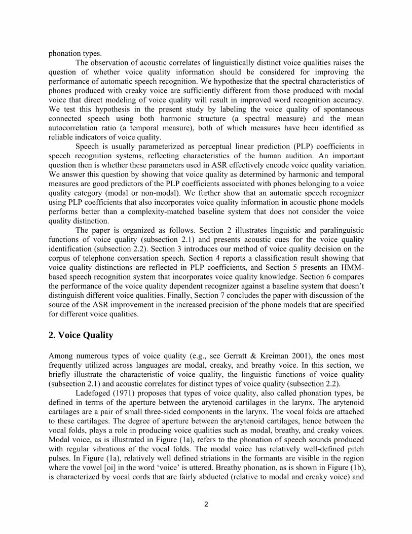
Ladefoged (1971) proposes that types of voice quality, also called phonation types, be defined in terms of the aperture between the arytenoid cartilages in the larynx. The arytenoid cartilages are a pair of small three-sided components in the larynx. The vocal folds are attached to these cartilages. The degree of aperture between the arytenoid cartilages, hence between the vocal folds, plays a role in producing voice qualities such as modal, breathy, and creaky voices. Modal voice, as is illustrated in Figure (1a), refers to the phonation of speech sounds produced with regular vibrations of the vocal folds. The modal voice has relatively well-defined pitch pulses. In Figure (1a), relatively well defined striations in the formants are visible in the region where the vowel [oi] in the word ‘voice’ is uttered. Breathy phonation, as is shown in Figure (1b), is characterized by vocal cords that are fairly abducted (relative to modal and creaky voice) and

3

have little longitudinal tension. The abduction and lowered tension allow turbulent airflow through the glottis. In Figure (1b), turbulent noise is present across the frequency range. Creaky phonation, as in Figure (1c), is typically associated with vocal folds that are tightly adducted but open enough along a portion of their length to allow for voicing. Due to the tight adduction, the creaky voice typically reveals slow and irregular vocal pulses in the spectrogram, as in Figure (1c), where the vocal pulses are farther apart from each other compared to those of modal and breathy voices in Figures (1a-b).

(a)

(b)

(c)

Figure 1: Spectrograms of the same word “voice” that are produced different phonations. From top to bottom, the word “voice” is produced with (a) modal voice, (b) breathy voice, and (c) creaky voice, respectively. (The sound files used for the spectrograms are taken from http://www.ims.uni-stuttgart.de/phonetik/EGG/.)

2.1. Functions of voice quality

4

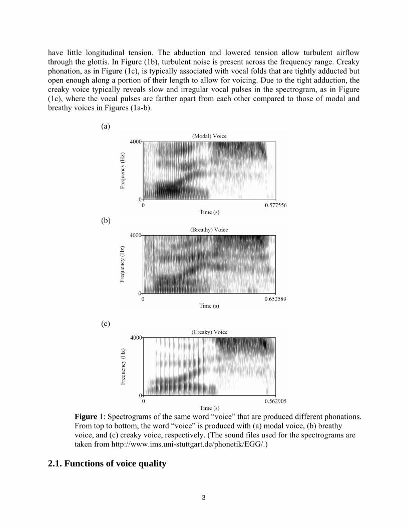
Voice quality distinctions are used in some languages to encode lexical contrast, and/or there may be allophonic variation in voice quality for some sounds. Voice quality also functions to signal the speaker’s emotional or attitudinal status, and to index socio-linguistic or extra-linguistic features. The function of voice quality varies depending on the language. The use of voice quality to encode lexical contrasts is fairly common in Southeast Asian, South African and Native American Languages. For example, the presence or absence of creakiness on the vowel a in “ϕα⇔” signals a difference in meaning in Jalapa Mazatec such that “ϕα0⇔” produced with creakiness means “he carries” whereas “ϕα⇔” produced without creakiness means “tree” (Ladefoged & Maddieson 1997; Gordon & Ladefoged 2001). Gujarati speakers need breathy voice or murmured voice to distinguish the word /βα−ρ/ produced with murmured voice “outside” from the word /bar/ “twelve” (Fischer-Jørgensen, 1967; Bickley, 1982; Gordon & Ladefoged 2001)1. Voice quality is also commonly used to encode allophonic variation in certain contexts. Thus, many languages use non-modal phonation of creaky or breathy voice as variants of modal voice in certain contexts. For example, voiceless stop /t/ in American English is often realized as glottal stop [?]. The spectrogram in Figure 2 illustrates that the final /t/ in the word “cat” is produced with glottal stop [?], with anticipatory non-modal phonation on the preceding vowel.

Figure 2: An allophonic realization of the voiceless stop /t/ as a glottal stop [?] (Figure taken from Epstein 2002)

A particular voice quality is often associated with specific tones in tonal languages.

Huffman (1987) observes that one of the seven tones in Hmong (a Sino-Tibetan language) is more likely to occur with a breathy voice quality. Jianfen & Maddieson (1989) describe that the yang tone in the Wu dialect of Chinese differs from the yin tone in that the yang tone is associated with the breathy voice.

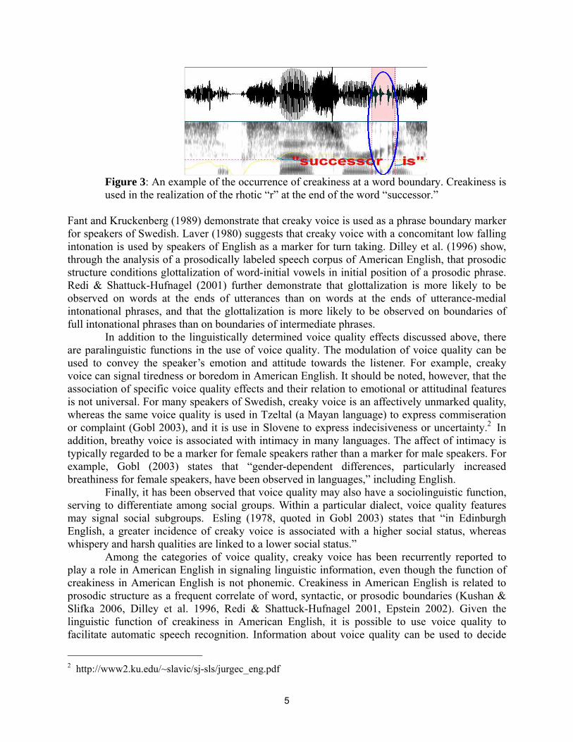
Voice quality can function as a marker for prosodic juncture. For example, creaky voice can be used to mark syllable, word, phrase, and utterance boundaries. Kushan & Slifka (2006) repot that 5% of their 1331 hand-labeled irregular phonation tokens in a subset of the TIMIT database occur at syllable boundaries, and 78% of the tokens at word boundaries. For example, creakiness is observed at the end of a word in Figure 3.

1 For a list of languages with different types of phonation contrasts, see Gordon & Ladefoged (2001).

5

Figure 3: An example of the occurrence of creakiness at a word boundary. Creakiness is used in the realization of the rhotic “r” at the end of the word “successor.”

Fant and Kruckenberg (1989) demonstrate that creaky voice is used as a phrase boundary marker for speakers of Swedish. Laver (1980) suggests that creaky voice with a concomitant low falling intonation is used by speakers of English as a marker for turn taking. Dilley et al. (1996) show, through the analysis of a prosodically labeled speech corpus of American English, that prosodic structure conditions glottalization of word-initial vowels in initial position of a prosodic phrase. Redi & Shattuck-Hufnagel (2001) further demonstrate that glottalization is more likely to be observed on words at the ends of utterances than on words at the ends of utterance-medial intonational phrases, and that the glottalization is more likely to be observed on boundaries of full intonational phrases than on boundaries of intermediate phrases.

In addition to the linguistically determined voice quality effects discussed above, there are paralinguistic functions in the use of voice quality. The modulation of voice quality can be used to convey the speaker’s emotion and attitude towards the listener. For example, creaky voice can signal tiredness or boredom in American English. It should be noted, however, that the association of specific voice quality effects and their relation to emotional or attitudinal features is not universal. For many speakers of Swedish, creaky voice is an affectively unmarked quality, whereas the same voice quality is used in Tzeltal (a Mayan language) to express commiseration or complaint (Gobl 2003), and it is use in Slovene to express indecisiveness or uncertainty.2 In addition, breathy voice is associated with intimacy in many languages. The affect of intimacy is typically regarded to be a marker for female speakers rather than a marker for male speakers. For example, Gobl (2003) states that “gender-dependent differences, particularly increased breathiness for female speakers, have been observed in languages,” including English.

Finally, it has been observed that voice quality may also have a sociolinguistic function, serving to differentiate among social groups. Within a particular dialect, voice quality features may signal social subgroups. Esling (1978, quoted in Gobl 2003) states that “in Edinburgh English, a greater incidence of creaky voice is associated with a higher social status, whereas whispery and harsh qualities are linked to a lower social status.”

Among the categories of voice quality, creaky voice has been recurrently reported to play a role in American English in signaling linguistic information, even though the function of creakiness in American English is not phonemic. Creakiness in American English is related to prosodic structure as a frequent correlate of word, syntactic, or prosodic boundaries (Kushan & Slifka 2006, Dilley et al. 1996, Redi & Shattuck-Hufnagel 2001, Epstein 2002). Given the linguistic function of creakiness in American English, it is possible to use voice quality to facilitate automatic speech recognition. Information about voice quality can be used to decide

2 http://www2.ku.edu/~slavic/sj-sls/jurgec_eng.pdf

6

between candidate analyses of an utterance by favoring analyses in which the syntactic and higher-level structures are consistent with the observed voice quality of a target word. In this way, voice quality constitutes a new channel of information to guide phrase-level analysis. An even more basic benefit of voice quality information is also possible: Voice quality effects condition substantial variation in the acoustic realization of a word or phone. Modeling that variation offers the possibility of improved accuracy in word or phone recognition. The next section details a method for reliably detecting creaky voice quality based on acoustic cues, independent of higher-level linguistic context, for the purpose of modeling creaky voice for speech recognition. 2.1. Acoustic correlates of voice quality Acoustic studies of voice quality effects have focused on analysis of F0 or intensity as acoustic correlates of voice quality (Gordon & Ladefoged 2001 and Gobl 2003). For example, segments with both breathy and creaky voices have been shown to have reduced intensity characteristics, and in languages such as Chong (Thongkum 1987) and Hupa (Gordon 1996), it is observed that phones produced with creakiness display a reduction in intensity relative to that of phones produced with modal phonation. However, intensity and F0 measures are not always reliable as cues to voice quality. For instance, intensity measurement is subject to many external factors such as the location of the microphone and background noise, and internal factors such as the speaker’s loudness level. Regarding F0, although slow and irregular vibration of the vocal folds often result in low F0 for creaky voice phones, F0 is not always a reliable indicator of voice quality. Studies of English have failed to show a strong correlation between any glottal parameters and F0 (Epstein, 2002).

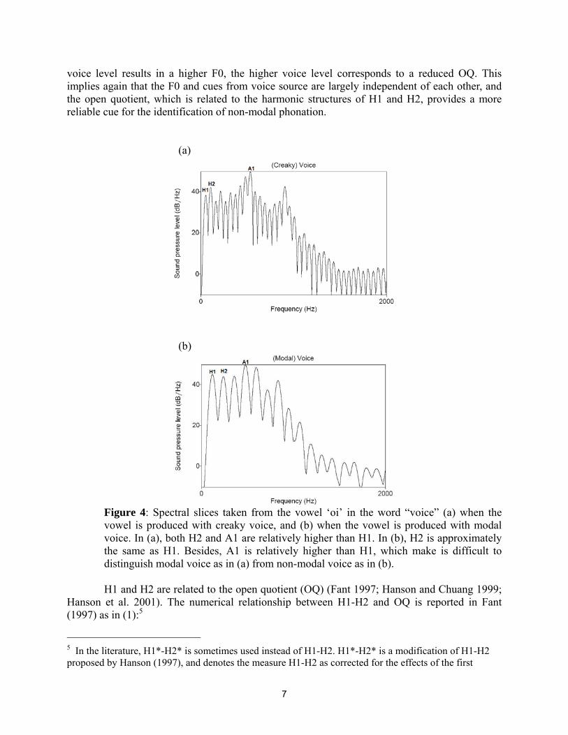
Information obtained from spectral structure is potentially more reliable than F0 or intensity for the purpose of voice quality identification. Ní Chasaide and Gobl (1997) characterize creaky phonation as having slow and irregular glottal pulses in addition to low F0. Specifically, they state that significant spectral cues to creaky phonation are i) A1 (i.e., amplitude of the strongest harmonic of the first formant) much higher than H1 (i.e., amplitude of the first harmonic)3, and ii) H2 (i.e., amplitude of the second harmonic) higher than H1.4 (See Figure 4 for an illustration.) Fisher-Jørgensen (1967) conducted a discrimination experiment between modal vowels and breathy vowels with Gujarati listeners using naturally produced Gujarati stimuli. The listeners were able to distinguish breathy vowels from modal ones in cases where the amplitude of the first harmonic dominates the spectral envelope. She observed that other cues such as f0 and duration had little importance in the task. Pierrehumbert (1989) investigated the interaction of prosodic events such as pitch accent and voice source variables. In general, the glottal pulse for high toned pitch accents has a greater open quotient than for low toned pitch accents. The open quotient (OQ) is defined as the ratio of the time in which the vocal folds are open to the total length of the glottal cycle. But it is also occasionally observed that while higher 3 The relative contribution of A1 in characterizing creaky voice is related to the increased bandwidth of the first formant. Hanson et al. (2001) states that “if the first-formant bandwidth (B1) increases, the amplitude A1 of the first-formant peak in the spectrum is expected to decrease. Therefore, the relative amplitude of the first harmonic and the first-formant peak (H1-A1, in dB) is selected as an indicator of B1.” Thus, the relative difference between H1-A1 is relevant to the discrimination between creaky voice and modal voice. 4 Some researchers use H1 and H2 to refer to individual harmonics, not to the amplitude of those harmonics. In this paper, H1 and H2 refer to the amplitude of the first and second harmonic, respectively.

7

voice level results in a higher F0, the higher voice level corresponds to a reduced OQ. This implies again that the F0 and cues from voice source are largely independent of each other, and the open quotient, which is related to the harmonic structures of H1 and H2, provides a more reliable cue for the identification of non-modal phonation. (a)

(b)

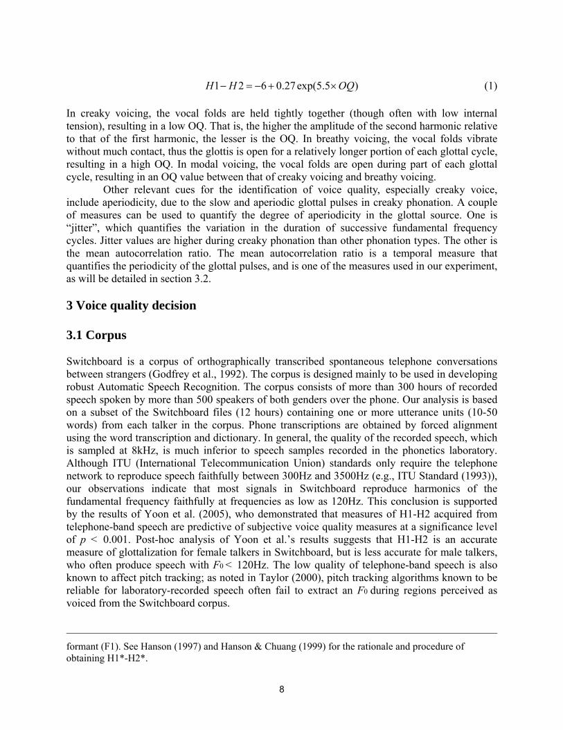
Figure 4: Spectral slices taken from the vowel ‘oi’ in the word “voice” (a) when the vowel is produced with creaky voice, and (b) when the vowel is produced with modal voice. In (a), both H2 and A1 are relatively higher than H1. In (b), H2 is approximately the same as H1. Besides, A1 is relatively higher than H1, which make is difficult to distinguish modal voice as in (a) from non-modal voice as in (b).

H1 and H2 are related to the open quotient (OQ) (Fant 1997; Hanson and Chuang 1999;

Hanson et al. 2001). The numerical relationship between H1-H2 and OQ is reported in Fant (1997) as in (1):5

5 In the literature, H1*-H2* is sometimes used instead of H1-H2. H1*-H2* is a modification of H1-H2 proposed by Hanson (1997), and denotes the measure H1-H2 as corrected for the effects of the first

8

1 2 6 0.27exp(5.5 )H H OQ− = − + × (1) In creaky voicing, the vocal folds are held tightly together (though often with low internal tension), resulting in a low OQ. That is, the higher the amplitude of the second harmonic relative to that of the first harmonic, the lesser is the OQ. In breathy voicing, the vocal folds vibrate without much contact, thus the glottis is open for a relatively longer portion of each glottal cycle, resulting in a high OQ. In modal voicing, the vocal folds are open during part of each glottal cycle, resulting in an OQ value between that of creaky voicing and breathy voicing.

Other relevant cues for the identification of voice quality, especially creaky voice, include aperiodicity, due to the slow and aperiodic glottal pulses in creaky phonation. A couple of measures can be used to quantify the degree of aperiodicity in the glottal source. One is “jitter”, which quantifies the variation in the duration of successive fundamental frequency cycles. Jitter values are higher during creaky phonation than other phonation types. The other is the mean autocorrelation ratio. The mean autocorrelation ratio is a temporal measure that quantifies the periodicity of the glottal pulses, and is one of the measures used in our experiment, as will be detailed in section 3.2. 3 Voice quality decision 3.1 Corpus Switchboard is a corpus of orthographically transcribed spontaneous telephone conversations between strangers (Godfrey et al., 1992). The corpus is designed mainly to be used in developing robust Automatic Speech Recognition. The corpus consists of more than 300 hours of recorded speech spoken by more than 500 speakers of both genders over the phone. Our analysis is based on a subset of the Switchboard files (12 hours) containing one or more utterance units (10-50 words) from each talker in the corpus. Phone transcriptions are obtained by forced alignment using the word transcription and dictionary. In general, the quality of the recorded speech, which is sampled at 8kHz, is much inferior to speech samples recorded in the phonetics laboratory. Although ITU (International Telecommunication Union) standards only require the telephone network to reproduce speech faithfully between 300Hz and 3500Hz (e.g., ITU Standard (1993)), our observations indicate that most signals in Switchboard reproduce harmonics of the fundamental frequency faithfully at frequencies as low as 120Hz. This conclusion is supported by the results of Yoon et al. (2005), who demonstrated that measures of H1-H2 acquired from telephone-band speech are predictive of subjective voice quality measures at a significance level of p < 0.001. Post-hoc analysis of Yoon et al.’s results suggests that H1-H2 is an accurate measure of glottalization for female talkers in Switchboard, but is less accurate for male talkers, who often produce speech with F0 < 120Hz. The low quality of telephone-band speech is also known to affect pitch tracking; as noted in Taylor (2000), pitch tracking algorithms known to be reliable for laboratory-recorded speech often fail to extract an F0 during regions perceived as voiced from the Switchboard corpus. formant (F1). See Hanson (1997) and Hanson & Chuang (1999) for the rationale and procedure of obtaining H1*-H2*.

9

3.2 Feature extraction and voice quality decision As mentioned above, the Switchboard corpus has the drawback that the recordings are band-limited signals. The voice quality of creakiness is correlated with low F0, which hinders accurate extraction of harmonic structure if the F0 falls below 120Hz. This is because harmonics are any whole-number multiple of F0. To enable a voice quality decision for signals with F0 below 120Hz, we use a combination of two measures: H1-H2 (a spectral measure, occasionally corrupted by the telephone channel) and mean autocorrelation ratio (a temporal measure, relatively uncorrupted by the telephone channel) in the decision algorithm for voice quality.

We use Praat (Boersma & Weenink 2005) to extract the spectral and temporal features that serve as cues to voice quality. First, intensity normalization is applied to each wave file. Following intensity normalization, inverse LPC filtering (Markel, 1972) is applied to remove effects of the vocal tract on source spectrum and waveform.

From the intensity-normalized, inverse-filtered signal, minimum F0, mean F0, and maximum F0 are derived over each file. These three values are used to set ceiling and floor thresholds for short-term autocorrelation F0 extraction, and to set a window that is dynamically sized to contain at least four glottal pulses. F0 and mean autocorrelation ratio are calculated on the intensity-normalized, inverse-filtered signal, using the autocorrelation method developed by Boersma (1993). The unbiased autocorrelation function rx(τ) of a speech signal x(t) over a window w(t) is defined as in (2):

( ) ( )

( )( ) ( )x

x t x t dtr

w t w t dt

ττ

τ

+≈

+∫∫

(2)

where τ is a time lag. The mean autocorrelation ratio is obtained by the following formula (3):

( )max(0)

xx

x

rrrτ

τ= (3)

where the angle brackets indicate averaging over all windowed segments, which are extracted at a timestep of 10ms. The range of the mean autocorrelation ratio is from 0 to 1, where 1 indicates a perfect match, and 0 indicates no match of the windowed signal and any shifted version. Harmonic structure is determined through spectral analysis using FFT and long term average spectrum (LTAS) analyses applied to the intensity-normalized, inverse filtered signal.

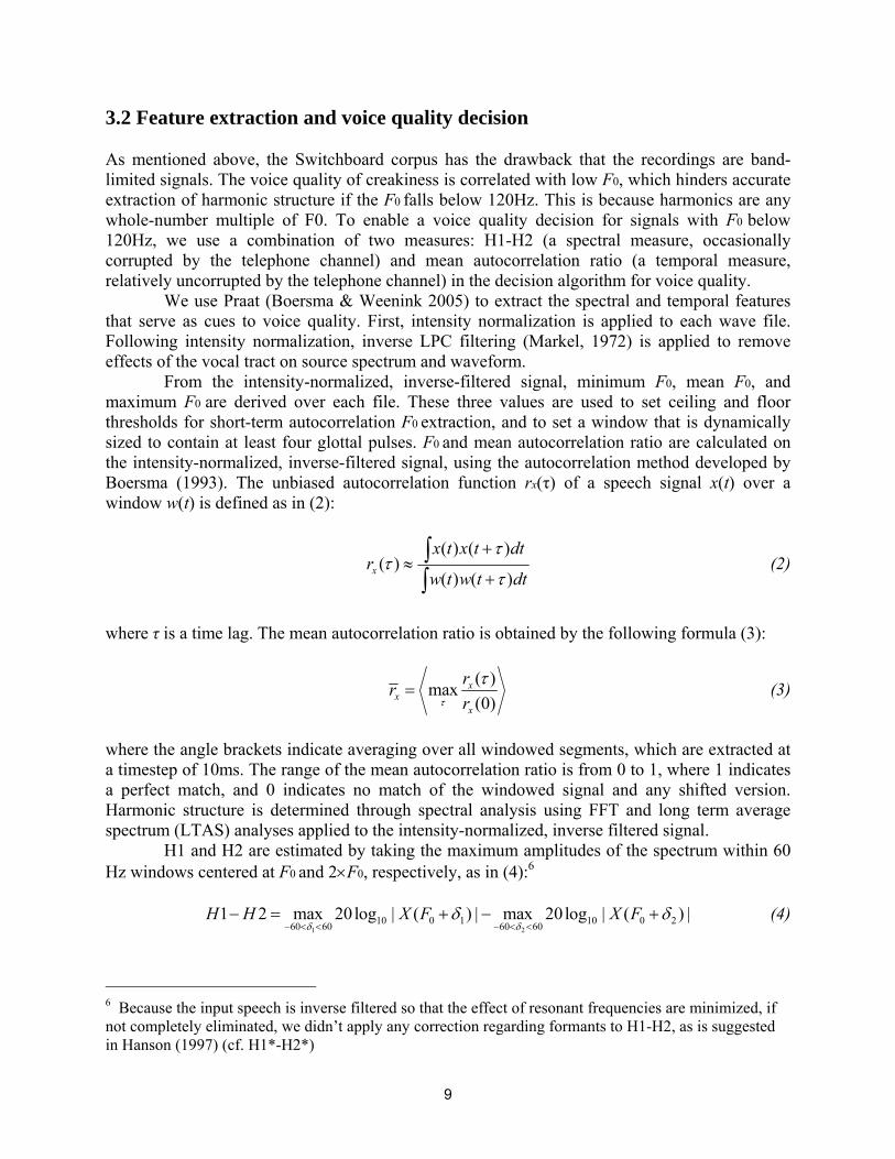
H1 and H2 are estimated by taking the maximum amplitudes of the spectrum within 60 Hz windows centered at F0 and 2×F0, respectively, as in (4):6

1 210 0 1 10 0 260 60 60 60

1 2 max 20log | ( ) | max 20log | ( ) |H H X F X Fδ δ

δ δ− < < − < <

− = + − + (4)

6 Because the input speech is inverse filtered so that the effect of resonant frequencies are minimized, if not completely eliminated, we didn’t apply any correction regarding formants to H1-H2, as is suggested in Hanson (1997) (cf. H1*-H2*)

10

where X(f) is the FFT spectrum at frequency f.

Yoon et al. (2005) previously used spectral features including H1-H2 to classify subjective voice quality with 75% accuracy. Subjective voice quality labels used in that experiment are not available for the research reported in this paper. In the current work, interactively-determined thresholds are used to divide the two-dimensional feature space [rx; H1-H2] into a set of voice-quality-related objective categories, as follows.

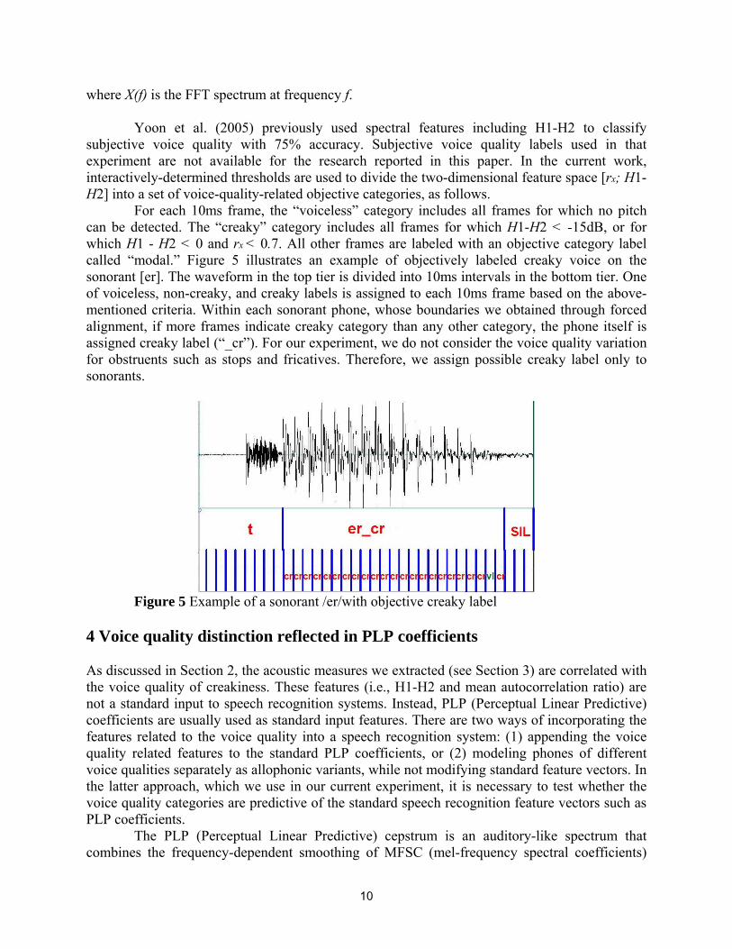
For each 10ms frame, the “voiceless” category includes all frames for which no pitch can be detected. The “creaky” category includes all frames for which H1-H2 < -15dB, or for which H1 - H2 < 0 and rx < 0.7. All other frames are labeled with an objective category label called “modal.” Figure 5 illustrates an example of objectively labeled creaky voice on the sonorant [er]. The waveform in the top tier is divided into 10ms intervals in the bottom tier. One of voiceless, non-creaky, and creaky labels is assigned to each 10ms frame based on the above-mentioned criteria. Within each sonorant phone, whose boundaries we obtained through forced alignment, if more frames indicate creaky category than any other category, the phone itself is assigned creaky label (“_cr”). For our experiment, we do not consider the voice quality variation for obstruents such as stops and fricatives. Therefore, we assign possible creaky label only to sonorants.

Figure 5 Example of a sonorant /er/with objective creaky label

4 Voice quality distinction reflected in PLP coefficients As discussed in Section 2, the acoustic measures we extracted (see Section 3) are correlated with the voice quality of creakiness. These features (i.e., H1-H2 and mean autocorrelation ratio) are not a standard input to speech recognition systems. Instead, PLP (Perceptual Linear Predictive) coefficients are usually used as standard input features. There are two ways of incorporating the features related to the voice quality into a speech recognition system: (1) appending the voice quality related features to the standard PLP coefficients, or (2) modeling phones of different voice qualities separately as allophonic variants, while not modifying standard feature vectors. In the latter approach, which we use in our current experiment, it is necessary to test whether the voice quality categories are predictive of the standard speech recognition feature vectors such as PLP coefficients.

The PLP (Perceptual Linear Predictive) cepstrum is an auditory-like spectrum that combines the frequency-dependent smoothing of MFSC (mel-frequency spectral coefficients)

11

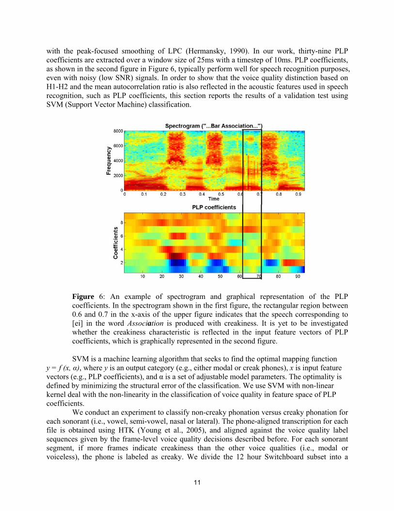
with the peak-focused smoothing of LPC (Hermansky, 1990). In our work, thirty-nine PLP coefficients are extracted over a window size of 25ms with a timestep of 10ms. PLP coefficients, as shown in the second figure in Figure 6, typically perform well for speech recognition purposes, even with noisy (low SNR) signals. In order to show that the voice quality distinction based on H1-H2 and the mean autocorrelation ratio is also reflected in the acoustic features used in speech recognition, such as PLP coefficients, this section reports the results of a validation test using SVM (Support Vector Machine) classification.

Figure 6: An example of spectrogram and graphical representation of the PLP coefficients. In the spectrogram shown in the first figure, the rectangular region between 0.6 and 0.7 in the x-axis of the upper figure indicates that the speech corresponding to [ei] in the word Association is produced with creakiness. It is yet to be investigated whether the creakiness characteristic is reflected in the input feature vectors of PLP coefficients, which is graphically represented in the second figure.

SVM is a machine learning algorithm that seeks to find the optimal mapping function

y = f (x, α), where y is an output category (e.g., either modal or creak phones), x is input feature vectors (e.g., PLP coefficients), and α is a set of adjustable model parameters. The optimality is defined by minimizing the structural error of the classification. We use SVM with non-linear kernel deal with the non-linearity in the classification of voice quality in feature space of PLP coefficients.

We conduct an experiment to classify non-creaky phonation versus creaky phonation for each sonorant (i.e., vowel, semi-vowel, nasal or lateral). The phone-aligned transcription for each file is obtained using HTK (Young et al., 2005), and aligned against the voice quality label sequences given by the frame-level voice quality decisions described before. For each sonorant segment, if more frames indicate creakiness than the other voice qualities (i.e., modal or voiceless), the phone is labeled as creaky. We divide the 12 hour Switchboard subset into a

12

training candidate pool (90%) and a testing candidate pool (10%). Then for each sonorant phone from the training candidate pool, we extract a subset of the non-creaky tokens that is equal in size to the creaky tokens for the same phone, based on the creakiness label resulting from the decision scheme. These non-creaky and creaky tokens compose the training data for each sonorant. The testing data for each sonorant are similarly generated from the testing candidate pool, which also have equal numbers of creaky and non-creaky tokens and no overlap with the training data. We use the SVM toolkit LibSVM (Chang and Lin, 2004), which implements a statistical learning technique for pattern classification, to perform supervised training of binary classifiers of creaky versus non-creaky phones for each sonorant, and tested the classification over the testing data, for each sonorant separately.

The classification accuracies obtained from the testing data for each sonorant are reported in Table 1. Our purpose here is to verify whether there are acoustic differences in the PLP coefficients that reflect the voice quality distinction we identify using the knowledge-based method described in the previous section. We do not attempt to optimize the SVM classification of creaky versus non-creaky phones in this experiment. Therefore, the default parameter setting of the radial basis function (RBF) in LibSVM is used without modification.

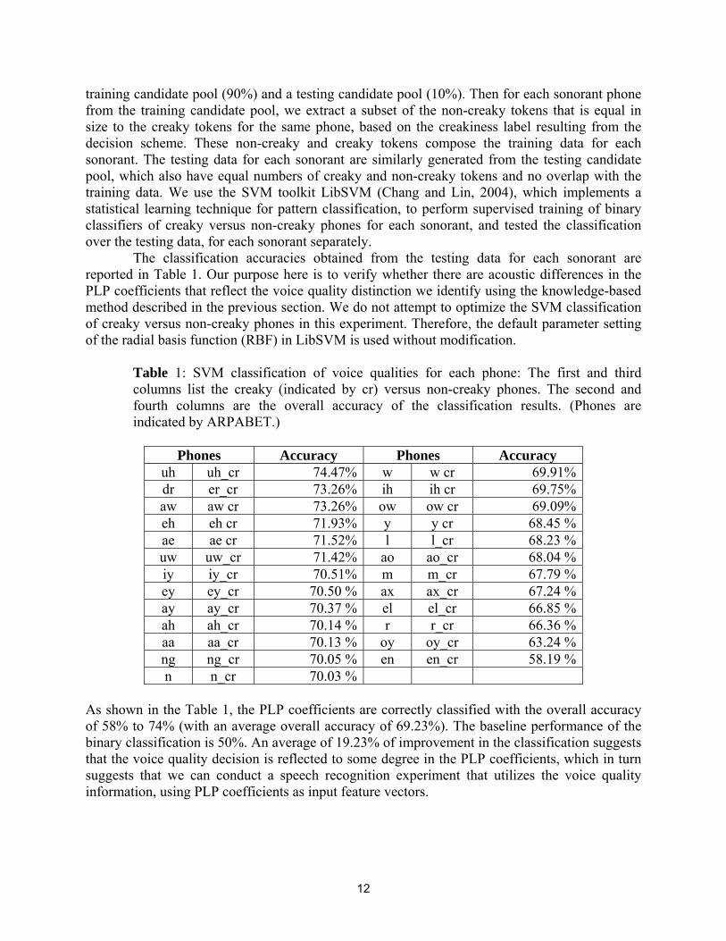
Table 1: SVM classification of voice qualities for each phone: The first and third columns list the creaky (indicated by cr) versus non-creaky phones. The second and fourth columns are the overall accuracy of the classification results. (Phones are indicated by ARPABET.)

Phones Accuracy Phones Accuracy

uh uh_cr 74.47% w w cr 69.91% dr er_cr 73.26% ih ih cr 69.75% aw aw cr 73.26% ow ow cr 69.09% eh eh cr 71.93% y y cr 68.45 % ae ae cr 71.52% l l_cr 68.23 % uw uw_cr 71.42% ao ao_cr 68.04 % iy iy_cr 70.51% m m_cr 67.79 % ey ey_cr 70.50 % ax ax_cr 67.24 % ay ay_cr 70.37 % el el_cr 66.85 % ah ah_cr 70.14 % r r_cr 66.36 % aa aa_cr 70.13 % oy oy_cr 63.24 % ng ng_cr 70.05 % en en_cr 58.19 % n n_cr 70.03 %

As shown in the Table 1, the PLP coefficients are correctly classified with the overall accuracy of 58% to 74% (with an average overall accuracy of 69.23%). The baseline performance of the binary classification is 50%. An average of 19.23% of improvement in the classification suggests that the voice quality decision is reflected to some degree in the PLP coefficients, which in turn suggests that we can conduct a speech recognition experiment that utilizes the voice quality information, using PLP coefficients as input feature vectors.

13

5 Voice quality dependent speech recognition The goal of a speech recognition system is to find the word sequence that maximizes the posterior probability of the word sequence 1 2( , , , ),Mw w w=W L given the observations

1 2( , , , )To o o=O L : ˆ arg max ( | )W p=

WW O (5)

Using Bayes rule and the fact that ( )p O is not affected by W ,

( | ) ( )ˆ arg max( )

arg max ( | ) ( )

p pWp

p p

=

=W

W

O W WO

O W W (6)

Sub-word units 1 2( , , , ),Lq q q=Q L such as phones, are usually essential to large vocabulary speech recognition, therefore we can rewrite formula (7) as:

ˆ arg max ( | ) ( )

arg max[max ( | ) ( | ) ( )]Q

W p p

p p p

=

≈W

W

O W W

O Q Q W W (7)

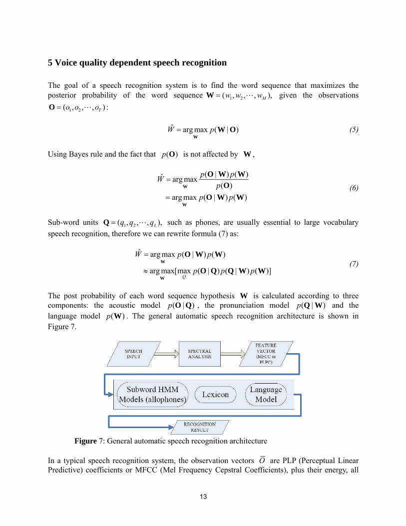
The post probability of each word sequence hypothesis W is calculated according to three components: the acoustic model ( | )p O Q , the pronunciation model ( | )p Q W and the language model ( )p W . The general automatic speech recognition architecture is shown in Figure 7.

Figure 7: General automatic speech recognition architecture

In a typical speech recognition system, the observation vectors O are PLP (Perceptual Linear Predictive) coefficients or MFCC (Mel Frequency Cepstral Coefficients), plus their energy, all

14

computed over a window size of 25ms at a time step of 10ms, and their first order and second order regression coefficients, referred to as delta and delta-delta coefficients.

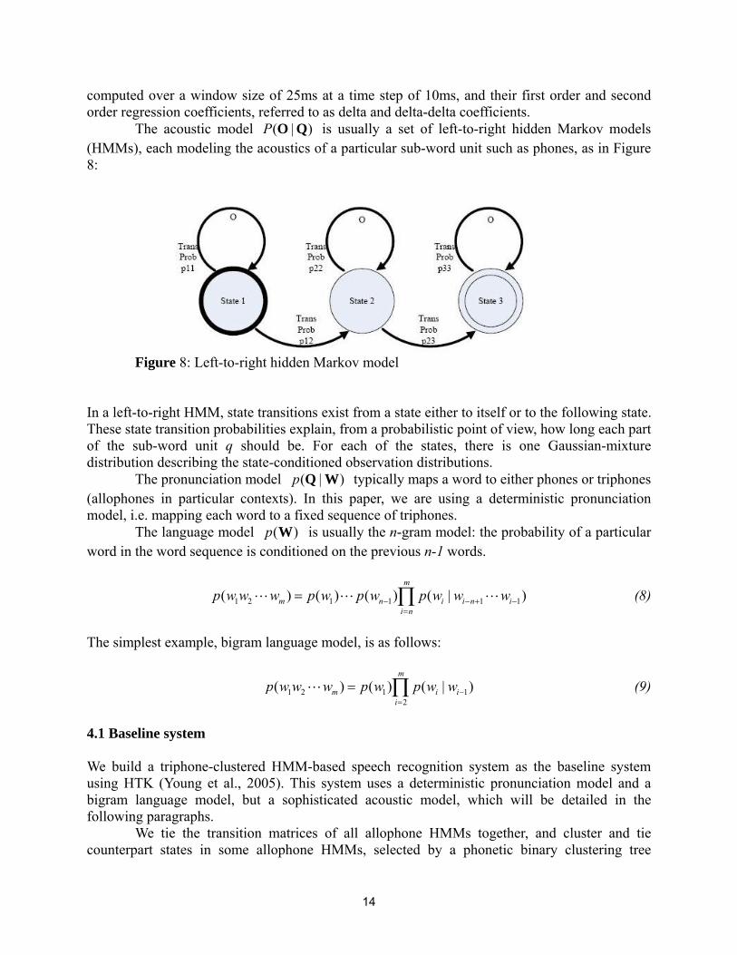
The acoustic model ( | )P O Q is usually a set of left-to-right hidden Markov models (HMMs), each modeling the acoustics of a particular sub-word unit such as phones, as in Figure 8:

Figure 8: Left-to-right hidden Markov model

In a left-to-right HMM, state transitions exist from a state either to itself or to the following state. These state transition probabilities explain, from a probabilistic point of view, how long each part of the sub-word unit q should be. For each of the states, there is one Gaussian-mixture distribution describing the state-conditioned observation distributions.

The pronunciation model ( | )p Q W typically maps a word to either phones or triphones (allophones in particular contexts). In this paper, we are using a deterministic pronunciation model, i.e. mapping each word to a fixed sequence of triphones. The language model ( )p W is usually the n-gram model: the probability of a particular word in the word sequence is conditioned on the previous n-1 words.

1 2 1 1 1 1( ) ( ) ( ) ( | )m

m n i i n ii n

p w w w p w p w p w w w− − + −=

= ∏L L L (8)

The simplest example, bigram language model, is as follows:

1 2 1 12

( ) ( ) ( | )m

m i ii

p w w w p w p w w −=

= ∏L (9)

4.1 Baseline system We build a triphone-clustered HMM-based speech recognition system as the baseline system using HTK (Young et al., 2005). This system uses a deterministic pronunciation model and a bigram language model, but a sophisticated acoustic model, which will be detailed in the following paragraphs.

We tie the transition matrices of all allophone HMMs together, and cluster and tie counterpart states in some allophone HMMs, selected by a phonetic binary clustering tree

15

(Figure 9).

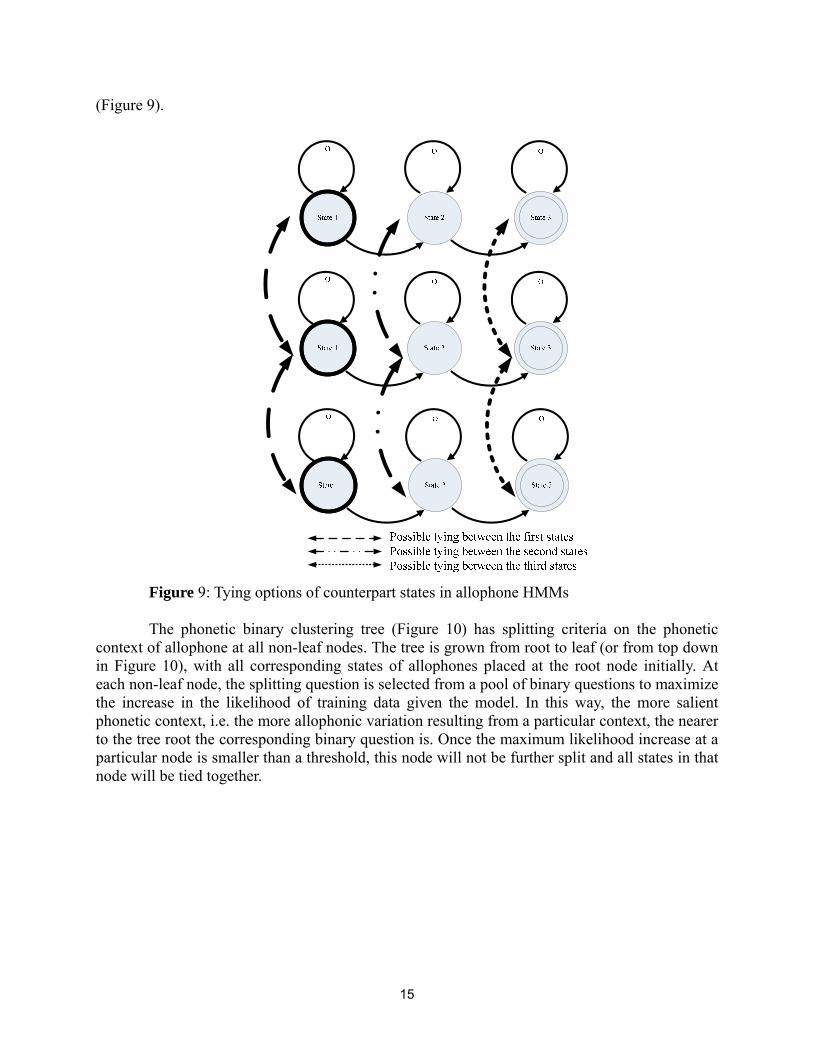
Figure 9: Tying options of counterpart states in allophone HMMs

The phonetic binary clustering tree (Figure 10) has splitting criteria on the phonetic

context of allophone at all non-leaf nodes. The tree is grown from root to leaf (or from top down in Figure 10), with all corresponding states of allophones placed at the root node initially. At each non-leaf node, the splitting question is selected from a pool of binary questions to maximize the increase in the likelihood of training data given the model. In this way, the more salient phonetic context, i.e. the more allophonic variation resulting from a particular context, the nearer to the tree root the corresponding binary question is. Once the maximum likelihood increase at a particular node is smaller than a threshold, this node will not be further split and all states in that node will be tied together.

16

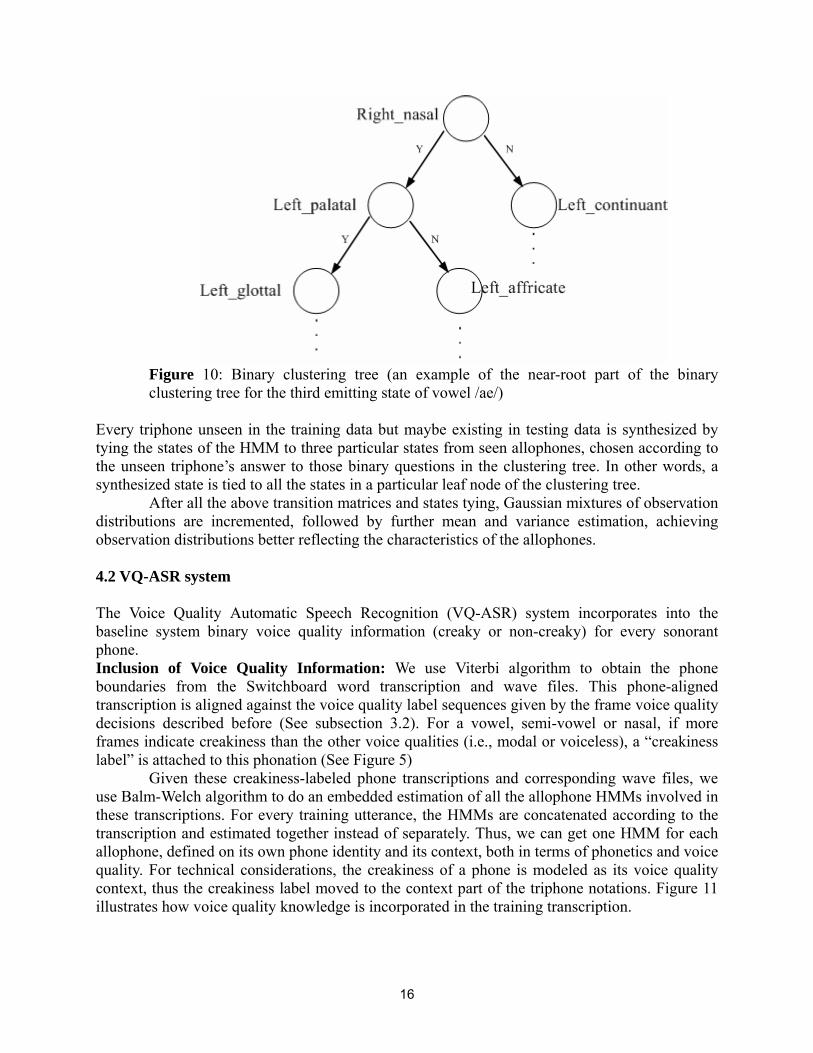
Figure 10: Binary clustering tree (an example of the near-root part of the binary clustering tree for the third emitting state of vowel /ae/)

Every triphone unseen in the training data but maybe existing in testing data is synthesized by tying the states of the HMM to three particular states from seen allophones, chosen according to the unseen triphone’s answer to those binary questions in the clustering tree. In other words, a synthesized state is tied to all the states in a particular leaf node of the clustering tree. After all the above transition matrices and states tying, Gaussian mixtures of observation distributions are incremented, followed by further mean and variance estimation, achieving observation distributions better reflecting the characteristics of the allophones. 4.2 VQ-ASR system The Voice Quality Automatic Speech Recognition (VQ-ASR) system incorporates into the baseline system binary voice quality information (creaky or non-creaky) for every sonorant phone. Inclusion of Voice Quality Information: We use Viterbi algorithm to obtain the phone boundaries from the Switchboard word transcription and wave files. This phone-aligned transcription is aligned against the voice quality label sequences given by the frame voice quality decisions described before (See subsection 3.2). For a vowel, semi-vowel or nasal, if more frames indicate creakiness than the other voice qualities (i.e., modal or voiceless), a “creakiness label” is attached to this phonation (See Figure 5)

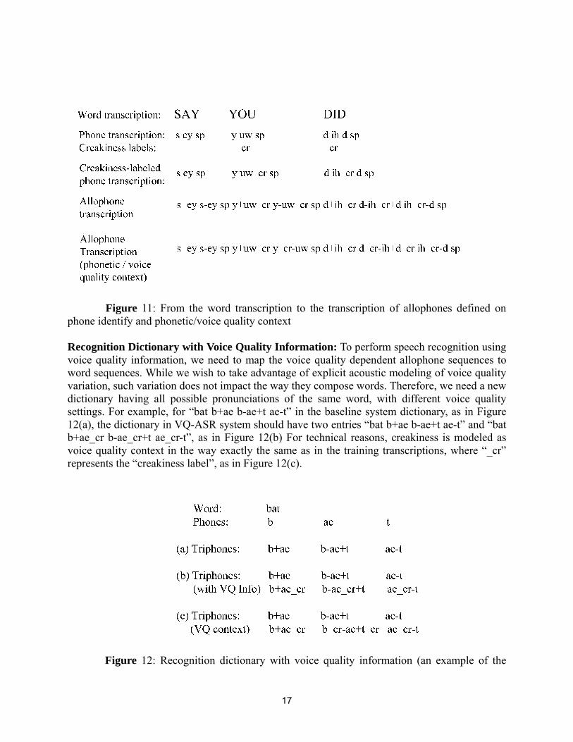
Given these creakiness-labeled phone transcriptions and corresponding wave files, we use Balm-Welch algorithm to do an embedded estimation of all the allophone HMMs involved in these transcriptions. For every training utterance, the HMMs are concatenated according to the transcription and estimated together instead of separately. Thus, we can get one HMM for each allophone, defined on its own phone identity and its context, both in terms of phonetics and voice quality. For technical considerations, the creakiness of a phone is modeled as its voice quality context, thus the creakiness label moved to the context part of the triphone notations. Figure 11 illustrates how voice quality knowledge is incorporated in the training transcription.

17

Figure 11: From the word transcription to the transcription of allophones defined on phone identify and phonetic/voice quality context Recognition Dictionary with Voice Quality Information: To perform speech recognition using voice quality information, we need to map the voice quality dependent allophone sequences to word sequences. While we wish to take advantage of explicit acoustic modeling of voice quality variation, such variation does not impact the way they compose words. Therefore, we need a new dictionary having all possible pronunciations of the same word, with different voice quality settings. For example, for “bat b+ae b-ae+t ae-t” in the baseline system dictionary, as in Figure 12(a), the dictionary in VQ-ASR system should have two entries “bat b+ae b-ae+t ae-t” and “bat b+ae_cr b-ae_cr+t ae_cr-t”, as in Figure 12(b) For technical reasons, creakiness is modeled as voice quality context in the way exactly the same as in the training transcriptions, where “_cr” represents the “creakiness label”, as in Figure 12(c).

Figure 12: Recognition dictionary with voice quality information (an example of the

18

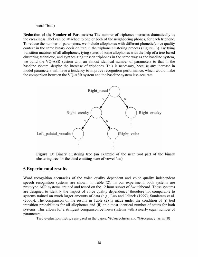
word “bat”) Reduction of the Number of Parameters: The number of triphones increases dramatically as the creakiness label can be attached to one or both of the neighboring phones, for each triphone. To reduce the number of parameters, we include allophones with different phonetic/voice quality context in the same binary decision tree in the triphone clustering process (Figure 13). By tying transition matrices of all allophones, tying states of some allophones with the help of a tree-based clustering technique, and synthesizing unseen triphones in the same way as the baseline system, we build the VQ-ASR system with an almost identical number of parameters to that in the baseline system, despite the increase of triphones. This is necessary, because any increase in model parameters will have a tendency to improve recognition performance, which would make the comparison between the VQ-ASR system and the baseline system less accurate.

Figure 13: Binary clustering tree (an example of the near root part of the binary clustering tree for the third emitting state of vowel /ae/)

6 Experimental results Word recognition accuracies of the voice quality dependent and voice quality independent speech recognition systems are shown in Table (2). In our experiment, both systems are prototype ASR systems, trained and tested on the 12 hour subset of Switchboard. These systems are designed to identify the impact of voice quality dependency, therefore not comparable to systems trained on much larger amounts of data (e.g., Luo and Jelinek (1999); Sundaram et al. (2000)). The comparison of the results in Table (2) is made under the condition of (i) tied transition probabilities for all allophones and (ii) an almost identical number of states for both systems. This allows for a stringent comparison between systems with a nearly equal number of parameters. Two evaluation metrics are used in the paper: %Correctness and %Accuracy, as in (8)

19

- -%Correctness= 100

- - -%Accuracy= 100

N D SN

N D S IN

×

× (10)

where N is the number of tokens (i.e. words) in the reference transcriptions that are usually reserved as a test dataset for the evaluation purpose, D, the number of deletion errors, S, the number of substitution errors, and I, the number of insertion errors. The %Correctness penalizes deletion errors and substitution errors deviating from reference transcriptions, and the %Accuracy further penalizes insertion errors in addition to the deletion and substitution errors. Word error rate (WER), another widely used evaluation metric, can be obtained with 100-%Accuracy.

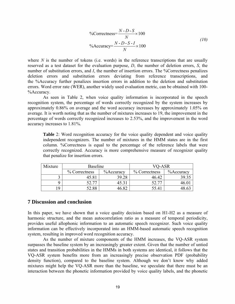
As seen in Table 2, when voice quality information is incorporated in the speech recognition system, the percentage of words correctly recognized by the system increases by approximately 0.86% on average and the word accuracy increases by approximately 1.05% on average. It is worth noting that as the number of mixtures increases to 19, the improvement in the percentage of words correctly recognized increases to 2.53%, and the improvement in the word accuracy increases to 1.81%.

Table 2: Word recognition accuracy for the voice quality dependent and voice quality independent recognizers. The number of mixtures in the HMM states are in the first column. %Correctness is equal to the percentage of the reference labels that were correctly recognized. Accuracy is more comprehensive measure of recognizer quality that penalize for insertion errors.

Baseline VQ-ASR Mixture % Correctness %Accuracy % Correctness %Accuracy

3 45.81 39.28 46.42 39.359 52.77 45.31 52.77 46.01

19 52.88 46.82 55.41 48.63 7 Discussion and conclusion In this paper, we have shown that a voice quality decision based on H1-H2 as a measure of harmonic structure, and the mean autocorrelation ratio as a measure of temporal periodicity, provides useful allophonic information to an automatic speech recognizer. Such voice quality information can be effectively incorporated into an HMM-based automatic speech recognition system, resulting in improved word recognition accuracy. As the number of mixture components of the HMM increases, the VQ-ASR system surpasses the baseline system by an increasingly greater extent. Given that the number of untied states and transition probabilities in the HMMs in both systems are identical, it follows that the VQ-ASR system benefits more from an increasingly precise observation PDF (probability density function), compared to the baseline system. Although we don’t know why added mixtures might help the VQ-ASR more than the baseline, we speculate that there must be an interaction between the phonetic information provided by voice quality labels, and the phonetic

20

information provided by triphone context. Perhaps the acoustic region represented by each VQ-ASR allophone is fully mapped out by a precise observation PDF to an extent not possible with standard triphones. Similar word recognition accuracy improvements have been shown for allophone models dependent on prosodic context (Borys, 2003). Glottalization has been shown to be correlated with prosodic context (e.g., Redi and Shattuck-Hufnagel (2001)), thus there is reason to believe that an ASR trained to be sensitive to both glottalization and prosodic context may have super-additive word recognition accuracy improvements. Acknowledgment This work is supported by NSF (IIS-0414117). Statements in this paper reflect the opinions and conclusions of the authors, and are not necessarily endorsed by the NSF. References BICKLEY, C. 1982. Acoustic analysis and perception of breathy vowels. Speech Communication

Group Working Papers, Research Laboratory of Electronics, MIT, 73-93. BOERSMA, P. 1993. Accurate short-term analysis of the fundamental frequency and the

harmonics-to-noise ratio of a sampling sound. In: Proceedings of the Institute of Phonetic Sciences. No. 17. University of Amsterdam.

BOERSMA, P., WEENINK, D. 2005. Praat: doing phonetics by computer (Version 4.3.19). [computer program], http://www.praat.org.

BORYS, S. 2003. The importance of prosodic factors in phoneme modeling with applications to speech recognition. In: HLT/NAACL student session. Edmonton.

CHANG, C.-C., LIN, C.-J. 2004. Libsvm: a library for support vector machine. System documentation, <http://www.csie.ntu.edu.tw/ ˜cjlin/libsvm>.

DILLEY, L., SHATTUCK-HUFNAGEL, S., OSTENDORF, M. 1996. Glottalization of word-initial vowels as a function of prosodic structure. Journal of Phonetics 24, 423–444.

EPSTEIN, M. A. 2002. Voice Quality and Prosody in English. Ph.D. dissertation, UCLA, California, LA.

FANT, G. 1960. Acoustic Theory of speech production. The Hague: Mouton FANT, G. 1999. The voice source in connected speech. Speech Communication 22, 125-139. FANT, G., KRUCKENBERG, A. 1989. Preliminaries to the study of Swedish prose reading and

reading style. STL-QPSR 2, 1-83, Speech, Music and Hearing, Royal Institute of Technology, Stockholm,

FISCHER-JØRGENSEN, E. 1967. Phonetic analysis of breathy (murmured) vowels. Indian Linguistics 28, 71-139.

GERRATT, B., KREIMAN, J. 2001. Towards a taxonomy of nonmodal phonation. Journal of Phonetics 29, 365–381.

GOBL, C. 2003. The Voice Source in Speech Communication: Production and Perception Experiments Involving Inverse Filtering and Synthesis. Ph.D. dissertation. Department of Speech, Music and Hearing. KTH, Stockholm, Sweden.

GODFREY, J., HOLLIMAN, E., MCDANIEL, J. 1992. Telephone speech corpus for research and development. In: Proceedings of ICASSP. San Francisco, CA.

GORDON, M. 1996. The phonetic structures of Hupa, UCLA Working Papers in Phonetics 93,

21

164-187. GORDON, M., LADEFOGED, P. 2001. Phonation types: a cross-linguistic overview. Journal of

Phonetics 29, 383–406. HANSON, H. 1997. Glottal characteristics of female speakers: acoustic correlates. Journal of the

Acoustical Society of America 101, 466-481. HANSON, H., CHUANG, E. 1999. Glottal characteristics of male speakers: Acoustic correlates and

comparison with female data. Journal of the Acoustical Society of America 106, 1697–1714.

HANSON, H., STEVENS, K.N., KUO, J., CHEN, M., & SLIFKA, J. 2001. Towards models of phonation. Journal of Phonetics 29, 451-480.

HERMANSKY, H. 1990. Perceptual linear predictive (plp) analysis of speech. Journal of the Acoustical Society of America 87 (4), 1738–1752.

HUFFMAN, M.K. 1987. Measures of phonation type in Hmong. Journal of the Acoustical Society of America 81, 495-504.

INTERNATIONAL TELECOMMUNICATION UNION (ITU) STANDARD G.711, 1993. Pulse code modulation (pcm) of voice frequencies.

JIANFEN, C., MADDIESON, I. 1989. An exploration of phonation types in Wu dialects of Chinese. UCLA Working Papers in Phonetics 72, 139-160.

KUSHAN, S., SLIFKA, J. 2006. Is irregular phonation a reliable cue towards the segmentation of continuous speech in American English? In: ICSA International Conference on Speech Prosody. Dresden, Germany.

LAVER, J. 1980. The Phonetic Description of Voice Quality. Cambridge, Cambridge University Press.

LUO, X., JELINEK, F. 1999. Probabilistic classification of hmm states for large vocabulary continuous speech recognition. In: IEEE International Conference on Acoustics, Speech, and Signal Processing. pp. 353–356.

MADDIESON, I., HESS, S. 1987. The effects of f0 of the linguistic use of phonation type. UCLA Working Papers in Phonetics 67, 112–118.

MARKEL, J. D. 1972. The sift algorithm for fundamental frequency estimation. IEEE Transactions on Audio and Electroacoustics 20 (5), 367–377.

NÍ CHASAIDE, A., GOBL, C. 1997. Voice source variation. In: Hardcastle,W., Laver, J. (Eds.), The Handbook of Phonetic Sciences. Blackwell Publishers, Oxford, pp. 1–11.

PIERREHUMBERT, J. 1989. A preliminary study of the consequences of intonation for the voice source. STL-QPSR, Speech, Music and Hearing, Royal Institute of Technology, Stockholm 4, 23-36.

REDI, L., SHATTUCK-HUFNAGEL, S. 2001. Variation in the rate of glottalization in normal speakers. Journal of Phonetics 29, 407–427.

SUNDARAM, R., GANAPATHIRAJU, A., HAMAKER, J., PICONE, J. 2000. ISIP 2000 conversational speech evaluation system. In: NIST Evaluation of Conversational Speech Recognition over the Telephone.

SWERT, M.; VELDHUIS, R. 2001. The effect of speech melody on voice quality. Speech Communication 33, 297-303.

TAYLOR, P. 2000. Analysis and synthesis of intonation using the tilt model. Journal of the Acoustical Society of America 107 (3), 1697–1714.

THONGKUM, T.L. 1987. Another look at the register distinction in Mon. UCLA Working Papers in Phonetics 67, 132-165.

22

YOON, T.-J., COLE, J., HASEGAWA-JOHNSON, M., SHIH, C. 2005. Acoustic correlates of nonmodal phonation in telephone speech. Journal of the Acoustical Society of America 117 (4), 2621.

YOUNG, S., EVERMANN, G., GALES, M., HAIN, T., KERSHAW, D., MOORE, G., ODELL, J., OLLASON, D., POVEY, D., VALTCHEV, V., WOODLAND, P. 2005. The HTK Book (version 3.3). Technical Report, Cambridge University Engineering Department, Cambridge, UK.

Tae-Jin Yoon Department of Linguistics, 4080 FLB University of Illinois at Urbana-Champaign 707 S. Mathews Ave. Urbana, IL 61801 U.S.A. tyoon@uiuc.edu Xiaodan Zhuang Department of Electrical and Computer Engineering University of Illinois at Urbana-Champaign 405 N. Mathews Ave. Urbana, IL 61801 U.S.A. xzhuang2@uiuc.edu Jennifer Cole Department of Linguistics, 4080 FLB University of Illinois at Urbana-Champaign 707 S. Mathews Ave. Urbana, IL 61801 U.S.A. jscole@uiuc.edu Mark Hasegawa-Johnson Department of Electrical and Computer Engineering University of Illinois at Urbana-Champaign 405 N. Mathews Ave. Urbana, IL 61801 U.S.A. jhasegaw@uiuc.edu