voice recognition system based on intra-modal fusion and
TRANSCRIPT
University of South FloridaScholar Commons
Graduate Theses and Dissertations Graduate School
2007
Voice recognition system based on intra-modalfusion and accent classificationSrikanth MangayyagariUniversity of South Florida
Follow this and additional works at: http://scholarcommons.usf.edu/etd
Part of the American Studies Commons
This Thesis is brought to you for free and open access by the Graduate School at Scholar Commons. It has been accepted for inclusion in GraduateTheses and Dissertations by an authorized administrator of Scholar Commons. For more information, please contact [email protected].
Scholar Commons CitationMangayyagari, Srikanth, "Voice recognition system based on intra-modal fusion and accent classification" (2007). Graduate Theses andDissertations.http://scholarcommons.usf.edu/etd/2274
brought to you by COREView metadata, citation and similar papers at core.ac.uk
provided by Scholar Commons | University of South Florida Research
Voice Recognition System Based on Intra-Modal Fusion and Accent Classification
by
Srikanth Mangayyagari
A thesis submitted in partial fulfillment of the requirements for the degree of
Master of Science in Electrical Engineering Department of Electrical Engineering
College of Engineering University of South Florida
Major Professor: Ravi Sankar, Ph.D. Sanjukta Bhanja, Ph.D.
Nagarajan Ranganathan, Ph.D.
Date of Approval: November 1, 2007
Keywords: Speaker Recognition, Accent Modeling, Speech Processing, Hidden Markov Model, Gaussian Mixture Model
© Copyright 2007, Srikanth Mangayyagari

DEDICATION
Dedicated to my parents who sacrificed their today for our better tomorrow.

ACKNOWLEDGMENTS
I would like to gratefully acknowledge the guidance and support of my thesis
advisor, Dr. Ravi Sankar, whose insightful comments and explanations have taught me a
great deal about speech and research in general. I am also grateful to Dr. Nagarajan
Ranganathan and Dr. Sanjukta Bhanja for serving on my committee. I would also like to
thank iCONS group members, especially Tanmoy Islam, for their valuable comments on
this work. I am indebted to USF biometric group and Speech Accent Archive (SAA) online
database group for providing the speech datasets for evaluation purposes. Finally, I would
like to thank my mother Nagamani, for her encouragement, support, and love.

i
TABLE OF CONTENTS
LIST OF TABLES …………………………………………………………………......... iv LIST OF FIGURES ……………………………………………………………………….v ABSTRACT …………………………………………………………………………….viii CHAPTER 1 INTRODUCTION ………………………………………………………...1 1.1 Background …………………………………………………………………..1
1.2 The Problem …………………………………………………………………. 5 1.3 Motivation ………………………………………………………………….... 8
1.4 Thesis Goals and Outline …………………………………………………..... 9
CHAPTER 2 HYBRID FUSION SPEAKER RECOGNITION SYSTEM …………… 12
2.1 Overview of Past Research ……………………………………………........ 12 2.2 Hybrid Fusion Speaker Recognition Model ………………………….......... 15 2.3 Speech Processing ......................................................................................... 16
2.3.1 Speech Signal Characteristics and Pre-Processing……………… 16
2.3.2 Feature Extraction ......................................................................... 22
2.4 Speaker models .............................................................................................. 26
2.4.1 Arithmetic Harmonic Sphericity (AHS) ....................................... 26 2.4.2 Hidden Markov Model (HMM) .................................................... 28
2.5 Hybrid Fusion ................................................................................................ 30
2.5.1 Score Normalization ..................................................................... 30

ii
2.5.2 Hybrid Fusion Technique ............................................................. 30
CHAPTER 3 ACCENT CLASSIFICATION SYSTEM .................................................33
3.1 Accent Background ....................................................................................... 33 3.2 Review of Past Research on Accent Classification ....................................... 34 3.3 Accent Classification Model ......................................................................... 38
3.4 Accent Features ............................................................................................. 39
3.5 Accent Classifier Formulation ....................................................................... 40
3.5.1 Gaussian Mixture Model (GMM) ................................................. 41 3.5.2 Continuous Hidden Markov Model (CHMM) .............................. 42
3.5.3 GMM and CHMM Fusion ............................................................ 44
CHAPTER 4 HYBRID FUSION – ACCENT SYSTEM ............................................... 46
4.1 Score Modifier Algorithm ............................................................................. 47 4.2 Effects of Accent Incorporation .................................................................... 49
CHAPTER 5 EXPERIMENTAL RESULTS .................................................................. 56
5.1 Datasets ..........................................................................................................56 5.2 Hybrid Fusion Performance ...........................................................................58
5.3 Accent Classification Performance ................................................................65
5.4 Hybrid Fusion - Accent Performance ............................................................ 67
CHAPTER 6 CONCLUSIONS AND FUTURE WORK ............................................... 72
6.1 Conclusions ....................................................................................................72 6.2 Recommendations for Future Research .........................................................74
REFERENCES ..................................................................................................................76

iii
APPENDICES .................................................................................................................. 80 Appendix A: YOHO, USF, AND SAA DATASETS………………………….......... 81 Appendix B: WORLD’S MAJOR LANGUAGES ...……………………………….. 83

iv
LIST OF TABLES Table 1 YOHO Dataset .......................................................................................... 81 Table 2 USF Dataset .............................................................................................. 81 Table 3 SAA (subset) Dataset ............................................................................... 82

v
LIST OF FIGURES Figure 1. Speaker Identification System .................................................................... 2 Figure 2. Speaker Verification System .......................................................................3 Figure 3. Current Speaker Recognition Performance over Various Datasets [3] ...... 6 Figure 4. Current Speaker Recognition Performance Reported by UK BWG [5] ..... 7 Figure 5. Flow Chart for Hybrid Fusion - Accent (HFA) Method ........................... 11 Figure 6. Flow Chart for Hybrid Fusion (HF) System ............................................. 16 Figure 7. Time Domain Representation of Speech Signal “Six” ..............................17 Figure 8. Framing of Speech Signal “Six” ............................................................... 18 Figure 9. Windowing of Speech Signal “Six” .......................................................... 19 Figure 10. Frequency Domain Representation - FFT of Speech Signal “Six” ...........21 Figure 11. Block Diagram for Computing Cepstrum ................................................. 22 Figure 12. Cepstrum Plots .......................................................................................... 23
Figure 13. Frequency Mapping Between Hertz and Mels ..........................................24
Figure 14. Mel-Spaced Filters .................................................................................... 25
Figure 15. Computation of MFCC ............................................................................. 25
Figure 16. Score Distributions ....................................................................................32 Figure 17. Block Diagram of Accent Classification (AC) System ............................ 39
Figure 18. Mel Filter Bank ......................................................................................... 40
Figure 19. Accent Filter Bank .................................................................................... 41

vi
Figure 20. Flow Chart for Hybrid Fusion – Accent (HFA) System ........................... 46
Figure 21. The Score Modifier (SM) Algorithm ........................................................ 48
Figure 22(a). Effect of Score Modifier – HF Score Histogram (Good Recognition Case) .......................................................................... 49 Figure 22(b). Effect of Score Modifier – HF Scores (Good Recognition Case) ............ 50
Figure 23(a). Effect of Score Modifier – HFA Score Histogram (Good Recognition Case) ..........................................................................................................51
Figure 23(b). Effect of Score Modifier – HFA Scores (Good Recognition Case) ..........51
Figure 24(a). Effect of Score Modifier – HF Score Histogram (Poor Recognition Case) ........................................................................... 51 Figure 24(b). Effect of Score Modifier – HF Scores (Poor Recognition Case) .............. 52
Figure 25(a). Effect of Score Modifier – HFA Score Histogram (Poor Recognition Case) ..........................................................................................................53
Figure 25(b). Effect of Score Modifier – HFA Scores (Poor Recognition Case) ........... 53 Figure 26(a). Effect of Score Modifier – HF Score Histogram (Poor Accent
Classification Case) .................................................................................. 54 Figure 26(b). Effect of Score Modifier – HF Scores
(Poor Accent Classification Case) ............................................................ 54 Figure 27(a). Effect of Score Modifier – HFA Score Histogram (Poor Accent
Classification Case) .................................................................................. 55 Figure 27(b). Effect of Score Modifier – HFA Scores (Poor Accent
Classification Case) .................................................................................. 55 Figure 28(a). ROC Comparisons of AHS, HMM, and HF systems for YOHO Dataset 59 Figure 28(b). ROC Comparisons of AHS, HMM, and HF Systems for USF Dataset .... 60 Figure 28(c). ROC Comparisons of AHS, HMM, and HF Systems for SAA Dataset ... 61 Figure 29. Comparison of AHS, HMM, and HF Recognition Rate at Various False
Acceptance Rates for YOHO Dataset ....................................................... 62

vii
Figure 30. Comparison of AHS, HMM, and HF Recognition Rate at Various False Acceptance Rates for USF Dataset ........................................................... 63
Figure 31. Comparison of AHS, HMM, and HF Recognition Rate at Various False
Acceptance Rates for SAA Dataset ...........................................................64 Figure 32. Accent Classification Rate Using Different Weight Factors for SAA and USF Datasets ...................................................................................... 66 Figure 33(a). ROC Comparisons for HF and HFA Methods Evaluated on SAA ........... 67 Figure 33(b). ROC Comparisons for HF and HFA Methods Evaluated on
USF Dataset ...............................................................................................69 Figure 34. Comparison of HFA and HF Recognition Rate at Various False
Acceptance Rates for SAA Dataset .......................................................... 70 Figure 35. Comparison of HFA and HF Recognition Rate at Various False
Acceptance Rates for USF Dataset ........................................................... 71 Figure 36 World’s Major Languages [30] ................................................................. 83

viii
VOICE RECOGNITION SYSTEM BASED ON INTRA-MODAL FUSION AND ACCENT CLASSIFICATION
Srikanth Mangayyagari
ABSTRACT
Speaker or voice recognition is the task of automatically recognizing people from their
speech signals. This technique makes it possible to use uttered speech to verify the speaker’s
identity and control access to secured services. Surveillance, counter-terrorism and homeland
security department can collect voice data from telephone conversation without having to
access to any other biometric dataset. In this type of scenario it would be beneficial if the
confidence level of authentication is high. Other applicable areas include online transactions,
database access services, information services, security control for confidential information
areas, and remote access to computers.
Speaker recognition systems, even though they have been around for four decades,
have not been widely considered as standalone systems for biometric security because of
their unacceptably low performance, i.e., high false acceptance and true rejection. This thesis
focuses on the enhancement of speaker recognition through a combination of intra-modal
fusion and accent modeling. Initial enhancement of speaker recognition was achieved
through intra-modal hybrid fusion (HF) of likelihood scores generated by Arithmetic
Harmonic Sphericity (AHS) and Hidden Markov Model (HMM) techniques. Due to the

ix
Contrastive nature of AHS and HMM, we have observed a significant performance
improvement of 22% , 6% and 23% true acceptance rate (TAR) at 5% false acceptance rate
(FAR), when this fusion technique was evaluated on three different datasets – YOHO, USF
multi-modal biometric and Speech Accent Archive (SAA), respectively. Performance
enhancement has been achieved on both the datasets; however performance on YOHO was
comparatively higher than that on USF dataset, owing to the fact that USF dataset is a noisy
outdoor dataset whereas YOHO is an indoor dataset.
In order to further increase the speaker recognition rate at lower FARs, we combined
accent information from an accent classification (AC) system with our earlier HF system.
Also, in homeland security applications, speaker accent will play a critical role in the
evaluation of biometric systems since users will be international in nature. So incorporating
accent information into the speaker recognition/verification system is a key component that
our study focused on. The proposed system achieved further performance improvements of
17% and 15% TAR at an FAR of 3% when evaluated on SAA and USF multi-modal
biometric datasets. The accent incorporation method and the hybrid fusion techniques
discussed in this work can also be applied to any other speaker recognition systems.

1
CHAPTER 1
INTRODUCTION
1.1 Background A number of major developments in several fields have occurred recently: the digital
computer, improvements in data-storage technology and software to code computer
programs, advanced sensor technology, and the derivation of a mathematical control theory.
All these developments have contributed to advancement of technology. But along with
advancement of technologies, security threats have increased in various realms such as
information, airport, home, international, and national securities. As of July 4th 2007, the
threat level from international terrorism is severe [1]. According to MSNBC, identity thefts
cost banks $1 billion per year and FBI estimates 500,000 victims in the year 2003 [2].
Identity theft is considered one of the country's fastest growing white-collar crimes. One
recent survey reported that there have been more than 28 million new identity theft victims
since 2003, but experts say many incidents go undetected or unreported. Due to the increased
level of security threats and fraudulent transactions, the need for reliable user authentication
has increased and hence biometric security systems have emerged. Biometrics, described as
the science of recognizing an individual based on his or her physical or behavioral traits, is
beginning to gain acceptance as a legitimate method for determining an individual’s identity.

2
Different biometrics that can be used are fingerprints, voice, iris scan, face, retinal scan,
DNA, handwriting typing patterns, gait, color of hair, skin, height, and weight of a person.
This research work focuses on voice biometrics or speaker recognition technology.
Speaker or voice recognition is the task of automatically recognizing people from
their speech signals. This technique makes it possible to use uttered speech to verify the
speaker’s identity and control access to secure services, i.e., online transactions, database
access services, information services, security control for confidential information areas,
remote access to computers, etc.
Figure 1. Speaker Identification System
A typical speaker recognition system is made up of two components: feature
extraction and classification. Speaker recognition (SR) can be divided into speaker
identification and speaker verification. Speaker identification system determines who
amongst a closed set of known speakers is providing the given utterance as depicted by the
Feature Extraction
Speaker 1 Model
Speaker N Model
Speaker 2 Model DecisionM
AX

3
block diagram in Figure 1. Speaker specific features are extracted from the speech data, and
compared with speaker models created from voice templates previously enrolled. The model
with which the features match the most is selected as the legitimate speaker. In most cases,
the model generates a likelihood score and the model that generates the maximum likelihood
score is selected.
Figure 2. Speaker Verification System
On the other hand, speaker verification system as depicted by the block diagram in
Figure 2, accepts or rejects the identity claim of a speaker. Features are extracted from
speech data and compared with the legitimate speaker model as well as an imposter speaker
model, which are created from previously enrolled data. The likelihood score generated from
the speaker model is subtracted from the imposter model. If the resultant score is greater than
a threshold value, then the speaker is accepted as a legitimate speaker. In either case, it is
expected that the persons using these systems are already enrolled. Besides these systems
Feature Extraction
Speaker Model
Imposter Model
Decision Σ
+
-
4
can be text-dependent or text-independent. Text-dependent system uses a fixed phrase for
training and testing a speaker. On the contrary, text-independent system does not use a fixed
phrase for training and testing purposes. In addition to security, speaker recognition has
various applications and is rapidly increasing. Some of the areas where speaker recognition
can be applied are [3]:
1) Access Control:
Secure physical locations as well as confidential computer databases can be accessed
through one’s voice. Access can also be given to private and restricted websites.
2) Online Transactions:
In addition to a pass phrase to access bank information or to purchase an item over the
phone, one’s speech signal can be used as an extra layer of security.
3) Law Enforcement:
Speaker recognition systems can be used to provide additional information for forensic
analysis. Inmate roll-call monitoring can be done automatically at prison.
4) Speech Data Management:
Voicemail services, audio mining applications, and annotation of recorded or live meetings
can use speaker recognition to label speakers automatically.
5) Multimedia and Personalization:
Soundtracks and music can be automatically labeled with singer and track information.
Websites and computers can be customized according to the person using the service.

5
1.2 The Problem
Even though speaker recognition systems have been researched over several decades and
have numerous applications, they still cannot match the performance of a human recognition
system [4] as well as not reliable enough to be considered as a standalone security system.
Although speaker verification is being used in many commercial applications, speaker
identification cannot be applied effectively for the same purpose. The performance of
speaker recognition systems degrade especially under different operating conditions. Speaker
recognition system performance is measured using various metrics such as recognition or
acceptance rate and rejection rate. Recognition rate deals with the number of genuine
speakers correctly identified, whereas rejection rate corresponds to the number of imposters
(people falsifying genuine identities) being rejected. Along with these performance metrics
there are some performance measures and trade-offs one needs to consider while designing
speaker recognition systems. Some of the performance measures generally used in the
evaluation of these systems include: false acceptance rate (FAR) - the rate at which an
imposter is accepted as a legitimate speaker, true acceptance rate (TAR) - the rate at which a
legitimate speaker is accepted, and false rejection rate (FRR) - the rate at which a legitimate
speaker is rejected (FRR=1-TAR).
There is a trade-off between FARs and TARs, as well as between FARs and FRRs.
Intuitively, as the false acceptance rate is increased, more speakers are accepted, and hence
true acceptance rate rises as well. But the chances of an imposter accessing the restricted
services also increase; hence a good speaker recognition system needs to deliver

6
performance even when the FAR threshold is lowered. The main problem in speaker
recognition is, poor TARs at lower FARs, as well as high FRRs.
The performance of a speaker recognition system [3] for three different datasets is
shown in Figure 3. Here, error (%) which is equivalent to FRR (%) has been used to measure
performance. The TIMIT dataset consists of clean speech from 630 speakers. As the dataset
is clean we can see that the error is almost zero, even though the number of people is
increased from 10 to 600. For NTIMIT, speech was acquired through telephone channels and
the performance degraded drastically as the speaker size was increased. At about 400
speakers we can see that the error is 35%, which means a recognition rate of 65%. We can
see the similar trend for SWBI dataset, where speech was also acquired through telephone
Figure 3. Current Speaker Recognition Performance over Various Datasets [3]
channel. However, the performance for SWBI is not as low as TIMIT, which indicates that
various other factors other than the type of acquisition influence the recognition rate. It

7
depends on the recording quality (environmental noise due to recording conditions and noise
introduced by the speakers such as lip smacks) and the channel quality. Hence it is hard to
generalize the performance of an SR system on a single dataset. From Figure 3, we can see
that the recognition rate degrades as the channel noise increases and also when the number of
speakers increases. Another evaluation of current voice recognition systems (Figure 4)
conducted by the UK BWG (Biometric Working Group) shows that about 95% recognition
can be achieved at an FAR of 1% [5]. The dataset consisted of about 200 speakers and voice
was recorded in a quiet office room environment.
Figure 4. Current Speaker Recognition Performance Reported by UK BWG [5]
On the whole, we can see that speaker recognition performance in a real world noisy
scenario cannot provide a high level of confidence. Speaker recognition systems can be
Performance of Voice Recognition
0
5
10
15
20 25
30
35
40
45
0.00 0.0 0.1 1 10 False Acceptance
Fals
e R
ejec
tion
Rat
e

8
considered reliable for both defense and commercial purposes, only if a promising
recognition rate is delivered at low FARs for realistic datasets.
1.3 Motivation
In this thesis, an effort has been made to deal with the problem, i.e. to achieve high TAR at
lower FARs even in realistic noisy conditions, by enhancing recognition performance with
the help of intra-modal fusion and accent modeling. The motivation behind the thesis can be
explained by answering the three questions: why enhance speaker recognition, why intra-
modal fusion and why combine accent information? In case of speaker recognition, obtaining
a person’s voice is non-invasive when compared to other biometrics, for example capture of
iris information. With very little additional hardware it is relatively easier to acquire this
biometric data. Recognition can be achieved even from long distance via telephones. In
addition surveillance, counter-terrorism and homeland security department can collect voice
data from telephone conversation without having to access to any other biometric dataset. In
this type of scenario it would be beneficial if the confidence level of authentication is high.
Previous research works in biometrics have shown recognition performance
improvements by fusing scores from multiple modalities such as face, voice, and fingerprint
[6], [7], [8]. However multi-modal systems have some limitations, i.e., cost of
implementation, availability of dataset, etc. On the other hand, by fusing two algorithms for
the same modality (intra-modal fusion), it has been observed in [8], that performance can be
similar to inter-modal systems when realistic noisy datasets are used. Intra-modal fusion
reduces complexity and cost of implementation when compared to various other biometrics,

9
such as fingerprint, face, iris, etc. Various additional hardware and data is required for
acquiring different biometrics of the same person.
Finally, speech is the most developed form of communication between humans.
Humans rely on several other types of information embedded within a speech signal, other
than voice alone. One of the higher levels of information that humans use is accent. Also,
incorporation of accent information provides us with a narrower search tool for the
legitimate speaker in huge datasets. In an international dataset, we can search within a pool
of dataset, where speakers belong to the same accent group as the legitimate speaker.
Homeland security, banks, and many other realistic entities, deal with users who are
international in nature. Hence incorporation of accent is a key for our speaker recognition
model.
1.4 Thesis Goals and Outline
The main goal in this thesis is to enhance speaker recognition system performance at lower
FARs with the help of an accent classification system, even when evaluated on a realistic
noisy dataset. The following are the secondary goals of this thesis:
1) Study the effect of intra-modal fusion of Arithmetic Harmonic Sphericity (AHS)
and Hidden Markov Model (HMM) speaker recognition systems.
2) Formulate a text-independent accent classification system.
3) Investigate accent incorporation into the fused speaker recognition system.
4) Evaluation of the combined speaker recognition system on a noisy dataset.
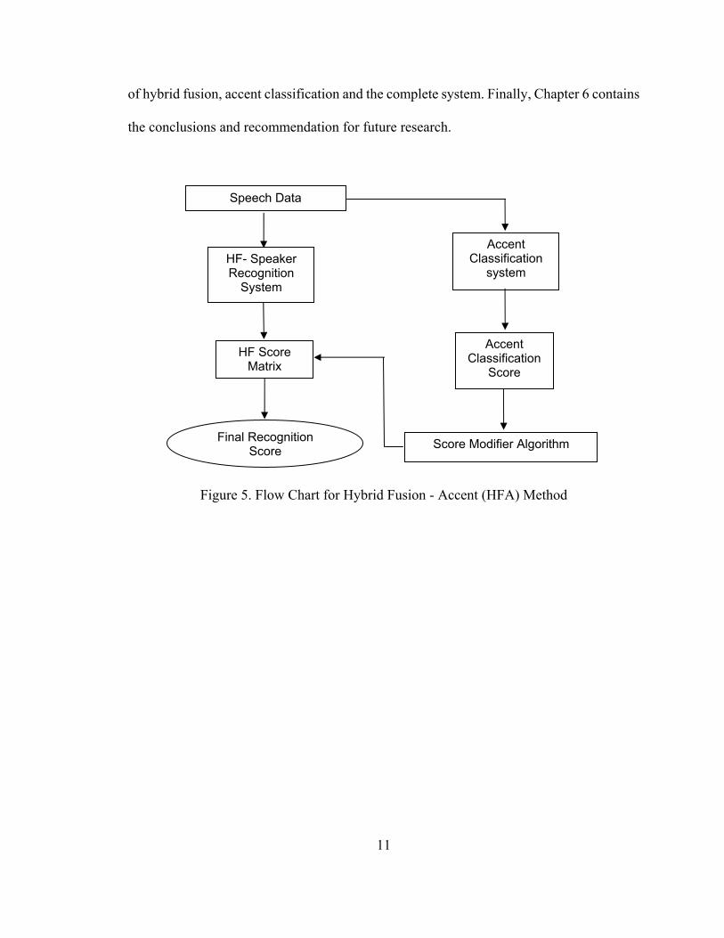
Figure 5 shows the flow chart of our proposed hybrid fusion – accent (HFA) method. We
have used the classification score from our accent classification system to modify the

10
recognition score obtained from our Hybrid Fusion (HF) speaker recognition system. Thus
the final enhanced recognition score is achieved. Our system consists of three parts – HF
system, AC system and the score modifier (SM) algorithm. The HF speaker recognition
system [9] is made up of score-level fusion of AHS [10] and HMM [11] models, which takes
enrolled and test speech data as inputs and generates a score as an output, which is a matrix
when a number of test speech inputs are provided. The accent classification system is made
up of a fusion of Gaussian mixture model (GMM) [12], and continuous hidden Markov
model (CHMM) [13], as well as a reference accent database. It accepts enrolled and test
speech inputs and generates an accent score and an accent class as the outputs for each test
data. The SM algorithm, a critical part of the proposed system, makes mathematical
modifications to the resultant HF score matrix controlled by the outputs of the accent
classification system. The final enhanced recognition scores are generated after the
modifications are made to the HF scores by the score modifier. Feature extraction is an
internal block within both the HF system as well as the accent classification (AC) system.
Each building block of the HFA system is studied in detail in the next sections.
The rest of the thesis is organized as follows. In the next sections each segment of the
HFA system is described thoroughly in the next chapters. The hybrid fusion speaker
recognition is explained in Chapter 2, which consists of background information of speech,
feature extraction, speaker model creation and the fusion technique used to fuse the speaker
recognition models. In Chapter 3, the accent classification system is described, along with
past research work in accent classification, accent feature, and the formulation of accent
classifier. In Chapter 4, the combination of speaker and accent models is investigated and its
effects are studied. Chapter 5 describes the datasets and shows the results and performances
11
of hybrid fusion, accent classification and the complete system. Finally, Chapter 6 contains
the conclusions and recommendation for future research.
Figure 5. Flow Chart for Hybrid Fusion - Accent (HFA) Method
HF- Speaker Recognition
System
HF Score Matrix
Final Recognition Score
Speech Data
Accent Classification
system
Accent Classification
Score
Score Modifier Algorithm

12
CHAPTER 2
HYBRID FUSION SPEAKER RECOGNITION SYSTEM
2.1 Overview of Past Research
Pruzansky at Bell labs in 1960 was one of the first ones to research on speaker recognition,
where he used filter banks and correlated two digital spectrograms for a similarity measure
[14]. P. D. Bricker and his colleagues experimented on text-independent speaker recognition
using averaged auto-correlation [15]. B. S. Atal studied the use of time domain methods for
text-dependent speaker recognition [16]. Texas Instruments came up with the first fully
automatic speaker verification system in the 1970’s. J. M. Naik and his colleagues
researched the usage of HMM techniques instead of template matching for text-dependent
speaker recognition [17]. In [18], text-independent speaker identification was studied based
on a segmental approach and mel-frequency cepstral coefficients were used as features. Final
decision and outlier rejection were based on a confidence measure. T. Matsui and S. Furui
investigated vector quantization (VQ) and HMM techniques to make speaker recognition
more robust [19]. Use of Gaussian mixture models (GMM) for text-independent speaker
recognition was successfully investigated by D. A. Reynolds and R. Rose [12]. Recent
research has focused on adding higher level information to speaker recognition systems to
increase the confidence level and to make them more robust. G. R. Doddington used
ideolectic features of speech such as word unigrams and bigrams to characterize a certain

13
speaker [20]. Evaluation was performed on the NIST extended data task which consisted of
telephone quality, long duration speech conversation from 400 speakers. An FRR of 40%
was observed at an FAR of 1%. In 2003, A. G. Adami used temporal trajectories of
fundamental frequencies and short term energies to segment and label speech which were
then used to model a speaker with the help of an N-gram model [21]. The same NIST
extended dataset was used and similar performance as in [20] was observed. In 2003, D. A.
Reynolds and his colleagues used high level information such as pronunciation models,
prosodic dynamics, pitch and duration features, phone streams and conversational
interactions, which were fused and modeled using an MLP to fuse N-grams, HMMs, and
GMMs [22]. The same NIST dataset was used for evaluation and a 98% TAR was observed
at 0.2% FAR. Also in 2006, a multi-lingual NIST dataset consisting of 310 speakers was
used for cross lingual speaker identification. Several speaker features derived from short
time acoustics, pitch, duration, prosodic behavior, phoneme and phone usage were modeled
using GMMs, SVMs, and N-grams [23]. The several modeling systems used in this work,
were fused using a multi layer perceptron (MLP). A recognition rate of 60% at an FAR of
0.2% has been reported. In [24], mel-frequency cepstral coefficients (MFCC) were modeled
using phonetically structured GMMs and speaker adaptive modeling. This method was
evaluated on YOHO consisting of clean speech from 138 speakers and Mercury dataset
consisting of telephone quality speech from 38 speakers. An error rate of 0.25% on YOHO
and 18.3% on Mercury were observed. In [25], MFCCs and their first order derivatives were
used as features and an MLP fusion of GMM-UBM system and speaker adaptive automatic
speech recognition (ASR) system were used to model these features. When evaluated on the

14
Mercury and Orion datasets consisting of 44 speakers in total, an FRR of 7.3% has been
reported. In [26], a 35 speaker NTT dataset was used for evaluating a fusion of a GMM
system and a syllable based HMM adapted by MAP system. MFCCs were used as features
and 99% speaker identification has been reported. In [27], SRI prosody database and NIST
2001 extended data task were used for evaluation. Though this paper was not explicitly
considering accent classification, it used a smoothed fundamental frequency contour (f0) at
different time scales as the features, which were then converted to wavelets by wavelet
analysis. The output distribution was then compacted and used to train a bigram for universal
background models (UBM) using a first order Markov chain. The log likelihood scores of
the different time scales were then fused to obtain the final score. The results indicate an 8%
equal error rate (where FAR is equal to FRR) for two utterance test segments and it degrades
to 18% when 20 test utterance segments were used. NIST 2001 extended data task
consisting of 482 speakers was used for evaluation. In [28], exclusive accent classification
was not performed, but formant frequencies were used for speaker recognition. Formant
trajectories and gender were used as features and a feed forward neural network was used for
classification. An average misclassification rate of 6.6% was observed for the six speakers
extracted from the TIMIT database.
In this thesis, we focused on an intra-modal speaker recognition system, to achieve
similar performance enhancement observed in [6], [7]. However, we used two
complementary voice recognition systems and fused their scores to have a better performing
system. Similar approach has been adopted in [24], [25] and [26], where scores from two
recognition systems were fused, one of the recognition algorithms was a variant of Gaussian

15
Mixture Model (GMM) [24] and the other being a speaker adapted HMM [26]. But, there are
a number of factors that differentiate this work from those described in [24], [25] and [26]:
Database size, data collection method, and the location of the data collected (indoor and
outdoor dataset). In [25] and [26], a small dataset, population of 44 and 35 respectively, was
used. We, on the other hand, conducted our experiment on two comparatively larger indoor
and outdoor datasets.
There has been a great deal of research towards improving speaker recognition rate
by adding supra-segmental, higher level information and some accent related features like
pronunciation models and prosodic information [21], [22], [27], [28]. But the effect of
incorporating the outcome of an accent modeling/classifying system into a speaker
recognition system has not been studied so far. Even though performance of the systems
reported in [21] and [22] was good, the algorithms were complex due to the utilization of
several classifiers with various levels of information fusion. But the system developed in this
thesis has relatively simpler algorithms compared to these higher level information fusion
systems.
2.2 Hybrid Fusion Speaker Recognition Model
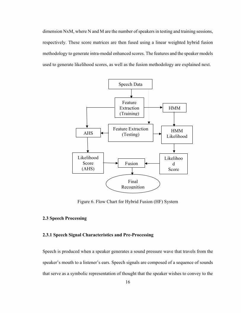
Figure 6 shows the flow chart of our proposed Hybrid Fusion (HF) method. We used same
person’s voice data from each dataset to extract features. Arithmetic Harmonic Sphericity
(AHS) is used to generate a similarity score between the enrolled feature and the test feature.
A Hidden Markov Model (HMM) is created from enrolled features and an HMM likelihood
score is generated for each test feature. The AHS and HMM likelihood score matrices are of
16
dimension NxM, where N and M are the number of speakers in testing and training sessions,
respectively. These score matrices are then fused using a linear weighted hybrid fusion
methodology to generate intra-modal enhanced scores. The features and the speaker models
used to generate likelihood scores, as well as the fusion methodology are explained next.
Figure 6. Flow Chart for Hybrid Fusion (HF) System
2.3 Speech Processing 2.3.1 Speech Signal Characteristics and Pre-Processing Speech is produced when a speaker generates a sound pressure wave that travels from the
speaker’s mouth to a listener’s ears. Speech signals are composed of a sequence of sounds
that serve as a symbolic representation of thought that the speaker wishes to convey to the
Feature Extraction(Training)
AHS
HMM
Feature Extraction(Testing)
HMM Likelihood
Likelihood
Score
Likelihood Score (AHS)
Fusion
Final Recognition
Speech Data

17
listener. The arrangement of these sounds is governed by a set of rules defined by the
language [29].
A speech signal must be sampled in order to make this data available to a digital
system as natural speech is analog in nature. Speech sounds can be classified into voiced,
unvoiced, mixed, and silence segments as shown in Figure 7, which is a plot of the sampled
speech signal “six”. Voiced sounds have higher energy levels and are periodic in nature
whereas unvoiced sounds are lower energy sounds and are generally non-periodic in nature.
Mixed sounds have both the features, but are mostly dominated by voiced sounds.
0 1000 2000 3000 4000 5000 6000 7000-1500
-1000
-500
0
500
1000
1500
2000
Samples
Am
plitu
de
Speech Signal "Six"
Figure 7. Time Domain Representation of Speech Signal “Six”
In order to distinguish speech of one speaker from the speech of another, we must use
features of the speech signal which characterize a particular speaker. In all speaker
Unvoiced
Voiced
Silence

18
recognition systems, several pre-processing steps are required before feature extraction and
classification. They are: pre-emphasis, framing, and windowing.
1) Pre-emphasis and Framing Pre-emphasis is the process of amplifying the high frequency, low energy unvoiced speech
signals. This process is usually performed using a simple first order high pass filter before
framing. As speech is a time-varying signal, it has to be divided into frames that possess
similar acoustic properties over short periods of time before features can be extracted.
Typically, a frame is 20-30 ms long where the speech signal can be assumed to be stationary.
One frame extracted from the speech data “six” is shown in Figure 8. It can be noted that the
signal is periodic in nature, because the extracted frame consists of voiced sound /i/.
0 50 100 150 200 250 300-1000
-500
0
500
1000
1500
Samples
Am
plitu
de
Frame Showing samples of /i/ from "Six"
Figure 8. Framing of Speech Signal “Six”

19
2) Windowing
The data truncation due to framing is equivalent to multiplying the input speech data with a
rectangular window function w(n) given by
1, n=0,1,.....N-1.( )
0, n otherwise.w n
⎧= ⎨⎩
(1)
Windowing leads to spectral spreading or smearing (due to increased main lobe width) and
spectral leakage (due to increased side lobe height) of the signal in the frequency domain. To
reduce spectral leakage, a smooth function such as Hamming window given by Equation (2)
is applied to each frame, at the expense of slight increase in spectral spreading (trade-off).
0.54 0.46 cos(2 n/N-1), n=0,1,.....N-1.( )
0, n otherwise.w n
π−⎧= ⎨⎩
(2)
0 50 100 150 200 250 3000
0.5
1Hamming Window
Samples
Am
plitu
de
0 50 100 150 200 250 300-1000
0
1000
2000Hamming Windowed Speech Signal "Six"
Am
plitu
de
Samples
Figure 9. Windowing of Speech Signal “Six”

20
As seen in the Figure 9, the middle portion of the signal is preserved whereas the beginning
and the end samples are attenuated as a result of using a Hamming window. In order to
have signal continuity and prevent data loss at the edges of the frames, the frames are
overlapped before further processing.
3) Fast Fourier Transform Fast Fourier Transform (FFT) is a name collectively given to several classes of fast
algorithms for computing the Discrete Fourier Transform (DFT). DFT provides a mapping
between the sequence, say x (n), n=0, 1, 2………, N-1 and a discrete set of frequency
domain samples, given by
1(2 / )
0( ) , k=0,1,.....N-1.
( )0, k otherwise.
Nj N kn
nx n e
X kπ
−−
=
⎧⎪= ⎨⎪⎩
∑ (3)
The inverse DFT (IDFT) is given by
1(2 / )
0
1 ( ) , n=0,1,.....N-1.( )
0, n otherwise.
Nj N kn
nX k e
x n Nπ
−
=
⎧⎪= ⎨⎪⎩
∑ (4)
Where, the IDFT is used map the frequency domain samples back to time domain samples.
The DFT is always is periodic in nature, where k varies from 1 to N, where N is the size of
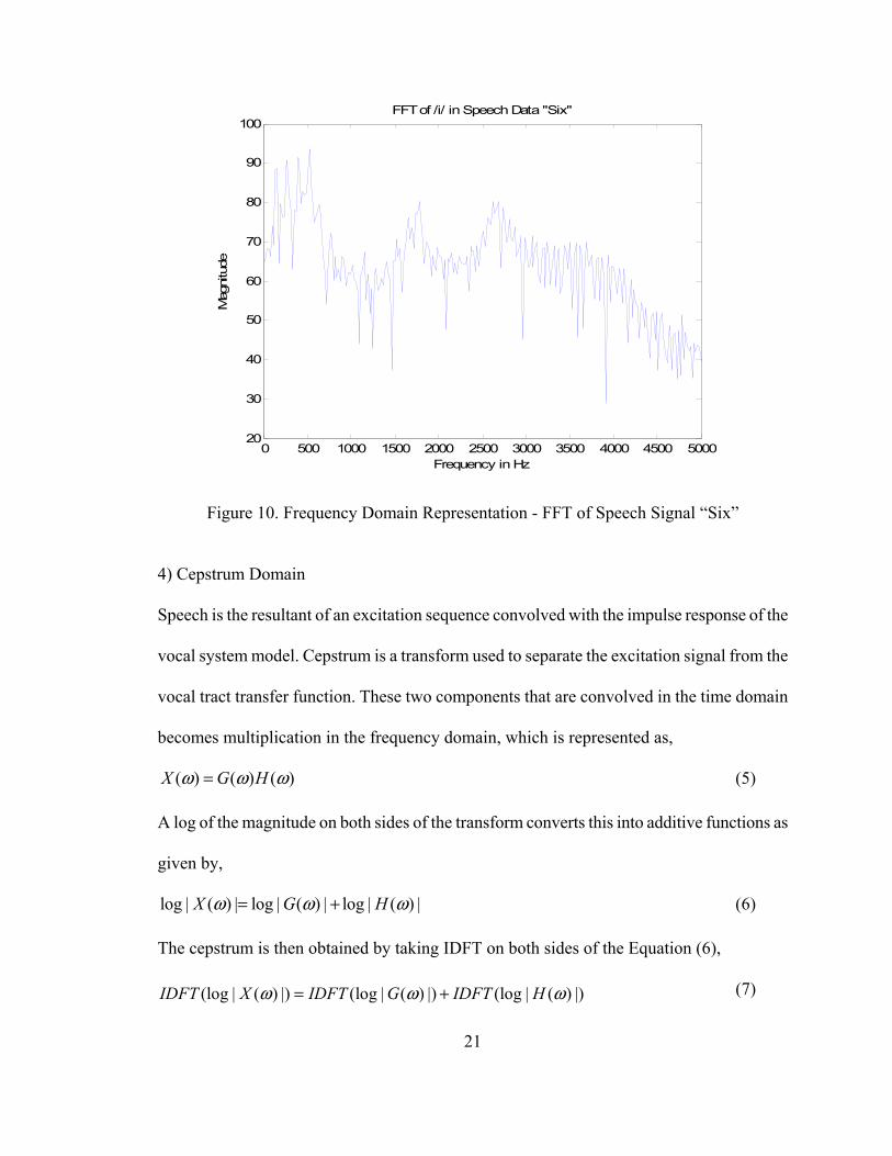
the DFT. The Figure 10 shows a 512-Point FFT for the speech data “six”.
21
0 500 1000 1500 2000 2500 3000 3500 4000 4500 500020
30
40
50
60
70
80
90
100
Frequency in Hz
Mag
nitu
de
FFT of /i/ in Speech Data "Six"
Figure 10. Frequency Domain Representation - FFT of Speech Signal “Six”
4) Cepstrum Domain
Speech is the resultant of an excitation sequence convolved with the impulse response of the
vocal system model. Cepstrum is a transform used to separate the excitation signal from the
vocal tract transfer function. These two components that are convolved in the time domain
becomes multiplication in the frequency domain, which is represented as,
( ) ( ) ( )X G Hω ω ω= (5)
A log of the magnitude on both sides of the transform converts this into additive functions as
given by,
log | ( ) | log | ( ) | log | ( ) |X G Hω ω ω= + (6)
The cepstrum is then obtained by taking IDFT on both sides of the Equation (6),
(7) (log | ( ) |) (log | ( ) |) (log | ( ) |)IDFT X IDFT G IDFT Hω ω ω= +

22
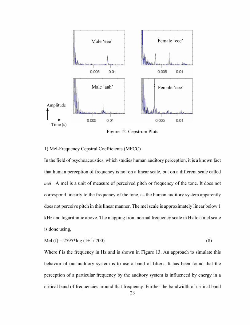
This process is better understood with the help of a block diagram (Figure 11). A lifter is
used to separate the high quefrency (Excitation) from the low quefrency (Transfer Function).
Figure 12 consists of the cepstral representations of sounds ‘eee’ and ‘aah’ uttered by male
and female speakers. We can see in the plot that the female speakers have higher peaks than
the male speakers, which is due to higher pitch of female speakers. The initial 5 ms consists
of the transfer function and the later part is the excitation.
Figure 11. Block Diagram for Computing Cepstrum
2.3.2 Feature Extraction Many speaker recognition systems use time domain features such as correlation, energy, and
zero crossings, frequency domain features such as formants and FFTs, as well as other
parametric features such as linear prediction coefficients (LPC) and cepstral coefficients.
Speech Signal Window
DFT
Abs |.|
Log
IDFT
Liftering
Excitation (High
Quefrency)
Transfer Function (Low Quefrency)
23
Figure 12. Cepstrum Plots
1) Mel-Frequency Cepstral Coefficients (MFCC) In the field of psychoacoustics, which studies human auditory perception, it is a known fact
that human perception of frequency is not on a linear scale, but on a different scale called
mel. A mel is a unit of measure of perceived pitch or frequency of the tone. It does not
correspond linearly to the frequency of the tone, as the human auditory system apparently
does not perceive pitch in this linear manner. The mel scale is approximately linear below 1
kHz and logarithmic above. The mapping from normal frequency scale in Hz to a mel scale
is done using,
Mel (f) = 2595*log (1+f / 700) (8)
Where f is the frequency in Hz and is shown in Figure 13. An approach to simulate this
behavior of our auditory system is to use a band of filters. It has been found that the
perception of a particular frequency by the auditory system is influenced by energy in a
critical band of frequencies around that frequency. Further the bandwidth of critical band
Male ‘eee’
Male ‘aah’
Female ‘eee’
Female ‘eee’
Amplitude
Time (s)

24
varies with frequency, beginning at about 100 Hz for frequencies below 1 kHz and then
increasing logarithmically above 1 kHz.
Figure 13. Frequency Mapping Between Hertz and Mels
A pictorial representation of the critical band of filters is shown in Figure 14. The
filter function depends on three parameters, the lower frequency fl, the central frequency fc
and the higher frequency fh. On a mel scale, the distances fc-fl and fh- fc are the same for each
filter and are equal to the distance between the fc’s of successive filters. The filter function
is:
( ) 0 and l hH f for f f f f= ≤ ≥ (9)
( ) ( ) /( ) l c l l cH f f f f f for f f f= − − ≤ ≤ (10)

25
( ) ( ) /( ) h h c c hH f f f f f for f f f= − − ≤ ≤ (11)
Figure 14. Mel-Spaced Filters
Figure 15. Computation of MFCC
As shown in Figure 15, the speech data is first extracted into 20-30 ms frames, next a
window is applied to each frame of data, and then it is mapped to the frequency domain
using FFT. Then the critical bands of filters are applied and are mel-frequency warped. In
order to convert the mel-frequency warped data to the cepstrum domain, we apply discrete
cosine transform since the MFCCs are real numbers. The MFCCs are given by,
1
1(log )cos , n=1,2,...,k2
k
n kk
c s n kkπ
=
⎡ ⎤⎛ ⎞= −⎜ ⎟⎢ ⎥⎝ ⎠⎣ ⎦∑ (12)
Speech Data
Frame Blocking
Window
FFT
Mel frequency Mapping
Discrete Cosine
TransformMel
Cepstrum
Mel Frequency Cepstral
Coefficients

26
Where cn are the MFCCs and sk is the mel power spectrum coefficients. Typically Cn values
are taken from 1 to 20, i.e. about 20 MFCCs for satisfactory results.
2.4 Speaker Models
The models Arithmetic Harmonic Sphericity (AHS) and Hidden Markov Model (HMM)
were used to model the MFCC features.
2.4.1 Arithmetic Harmonic Sphericity (AHS)
According to Gaussian Speaker Modeling [10], a speaker X’s speech characterized with a
feature vector sequence, xt can be modeled by its mean vector x and covariance matrix
X i.e.
1 1
1 1 and ( ).( )M M T
t t tt t
x x X x x x xM M= =
∑ ∑= = − − (13)
Where, M is the length of the vector sequence tx .
Similarly a speaker Y’s speech can be modeled by,
1 1
1 1 and ( ).( )N N T
t t tt t
y y Y y y y yN N= =
∑ ∑= = − − (14)
Where, N is the length of the vector sequence ty , y the mean vector and Y , the covariance
matrix.
Also, vectors x and y have a dimension of p , whereas the matrices X and Y are
p p× dimensional. We also express iλ as the eigen values of the matrixτ , where1 i p< < , i.e.,
Det[τ - λ I]=0 (15)

27
Where Det is the determinant, I is the Identity matrix and 1/ 2 1/ 2X YXτ − −= , where X and Y are
the covariance matrices.
Matrix τ can be written as,
1τ −= ΘΔΘ (16)
Where Θ , is the p p× diagonal matrix of eigen values and Δ is the matrix of eigen vectors.
Mean functions of these eigen values are given by,
Arithmetic mean: 1,1
1( ......, )p
p ii
ap
λ λ λ=∑= (17)
Geometric mean: ( )1/
1,1
( ......, )pp
p ii
g λ λ λ=∏= (18)
Harmonic mean: 1
1,1
1 1( ......, )p
pi i
hp
λ λλ
−
=∑
⎛ ⎞= ⎜ ⎟⎝ ⎠
(19)
These means can also be calculated directly using the covariance matrices, because of the
trace and determinant properties of matrices, which states that trace(XY)=trace(YX),
Det(XY)=Det(X).Det(Y), we have
11,
1 1 1( ......, ) ( ) ( ) ( )pa tr tr tr YXp p p
λ λ τ −= Δ = = (20)
( ) ( )1/
1/ 1/1,
( )( ......, ) ( ) ( )( )
pp p
pDet Yg Det DetDet X
λ λ τ ⎛ ⎞= Δ = = ⎜ ⎟
⎝ ⎠ (21)
1, 1 1 1( ......, )( ) ( ) ( )pp p ph
tr tr tr XYλ λ
τ− − −= = =Δ
(22)
The Arithmetic Harmonic Sphericity measure is a likelihood measure for verifying the
proportionality of covariance matrix Y to a given covariance matrix X , given by

28
/ 2 / 2
1/ 2 1/ 2
1/ 2 1/ 2
( ) ( )( | )
( ) ( )
N N
Det X YX DetS Y X p ptr X YX tr
τ
τ
− −
− −
⎡ ⎤ ⎡ ⎤⎢ ⎥ ⎢ ⎥
= =⎢ ⎥ ⎢ ⎥⎢ ⎥ ⎢ ⎥⎢ ⎥ ⎢ ⎥⎣ ⎦ ⎣ ⎦
(23)
By denoting, XS as the average likelihood function for the sphericity test, we have
1 log ( | )XS S Y XN
= (24)
and by defining,
1 ( )(X,Y) log
( )
trp
ptr
τμ
τ
⎡ ⎤⎢ ⎥
= ⎢ ⎥⎢ ⎥⎢ ⎥⎣ ⎦
(25)
1/ 2 1/ 2
1/ 2 1/ 2
1 ( )(X,Y) log
( )
tr X YXp
ptr Y XY
μ
− −
− −
⎡ ⎤⎢ ⎥
= ⎢ ⎥⎢ ⎥⎢ ⎥⎣ ⎦
(26)
1/ 2 1/ 2 1/ 2 1/ 2
2
( )* ( )(X,Y) log tr X YX tr Y XYp
μ− − − −⎡ ⎤
= ⎢ ⎥⎣ ⎦
(27)
1 1(X,Y) log[ ( )* ( )] 2 log[ ]tr X Y tr Y X pμ − −= − (28)
Where, (X,Y)μ is the log ratio of arithmetic and harmonic means of the eigen values of the
covariance matrices X andY . (X,Y)μ is the AHS similarity or distance measure which
indicates the resemblance between the enrolled and test features.
2.4.2 Hidden Markov Model (HMM) HMM has been widely used for modeling speech recognition systems and it can also be
extended for speaker recognition systems. Let an observation sequence be O= (o1 o…. oT)

29
and its HMM model be λ= (A, B, π). Where A denotes state transition probability, B denotes
output probability density functions, and π is the initial state probabilities. We can iteratively
optimize the model parameters λ, so that it best describes the given observation O. Thus the
likelihood (Expectation), P(O|λ) is maximized. This can be achieved using Baum-Welch
method, also known as Expectation Maximization (EM) algorithm [11].
To re-estimate HMM parameters, ( , )t i jξ is defined as the probability of being in state i at
time t, and state j at time t+1, given the model and the observation sequence,
1( , | , )( , )( | )
t tt
P q i q j Oi jP O
λξλ
+= == (29)
Using above formula, we can re-estimate HMM parameter
λ = (A, B, π) by
1( )j iπ γ= (30)
1 1
1 1 ( , ) / ( )T T
t tij t ta i j iξ γ− −
∑ ∑= =
= (31)
. .1 1
( ) ( ) ( )/s t o vt k
T Tt tj t t
b k j jγ γ=
∑ ∑= =
= (32)
Where1
( ) ( , )N
t tji i jγ ξ∑
== .
Thus we can iteratively find optimal HMM parameter λ [8]. This procedure is also viewed as
training since using optimal HMM parameter model we can later compare a testing set of
data or observation O by calculating the likelihood P(O|λ).
Thus AHS and HMM likelihood scores are generated, but in order to fuse these
scores we need to bring both scores to the same level, hence we need to normalize them.

30
2.5 Hybrid Fusion
2.5.1 Score Normalization
The score matrices generated by AHS and HMM are denoted as ijAHSS and ij
HMMS ;
1 i m≤ ≤ and1 j n≤ ≤ , respectively, where m is the number of speakers used in training session
and n is the number of speakers in testing session. These scores are in different scales and
have to be normalized, before they can be fused together, so that both the scores are
relatively in the same scale. We have used Min-Max normalization, therefore scores of AHS
and HMM are scaled between zero and one.
These normalized scores can be represented as follows,
min( )
max( ) min( )
ijS SS
S S
−=
− (33)
Where S is the normalized scores obtained from AHS or HMM. Though these scores are
between zero and one, their distributions are not similar. A deeper insight into the
distributions shows that AHS has wider distribution range when compared to HMM, which
has a narrower distribution.
2.5.2 Hybrid Fusion Technique
Figures 16(a) and 16(c) show the genuine score distribution of the AHS and HMM, while
Figures 16(b) and 16(d) show the imposter distribution of AHS and HMM algorithm,
respectively. It can be seen that distributions among AHS and HMM are clearly different.
The imposter and genuine distribution of AHS is well spread out, but the imposter
distribution has a Gaussian like shape. On the other hand, the distributions of HMM, are

31
closely bound. In a good recognition system, the genuine distribution is closely bound and
stands separated from that of the imposter which is spread out and similar to a Gaussian in
shape.
Thus in order to obtain the best score from both these methods; we have to use the
complementary nature of the algorithms. We used a linear weighted fusion method derived
as follows,
(( ) )opt HMM AHS AHSS S S Sω= − × + (34)
In order to find the weight, we used an enhanced weighting method. The weightω , is
calculated using the mean of the scores,
AHS
AHS HMM
MM M
ω =+
(35)
Here, HMMM , AHSM are the means of normalized scores from AHS and HMM, given as,
1 1
11 1 1
m n ij
j i
i mM S
j nm n= =∑ ∑
≤ ≤⎡ ⎤= ⎢ ⎥ ≤ ≤⎣ ⎦ (36)
Thus the features (MFCCs) are extracted, and these features are modeled using HMM and
AHS systems. The scores from these two models are fused to produce the final output score
of the HF speaker recognition system.

32
(a) (b)
(c) (d)
Figure 16. Score Distributions. (a) & (c) Genuine Distribution Generated Using AHS and
HMM, Respectively. (b) & (d) Imposter Distribution Generated Using AHS and HMM,
Respectively.
33
CHAPTER 3
ACCENT CLASSIFICATION SYSTEM
Before we proceed towards the accent features and modeling algorithms used in the
proposed AC system, a brief background and a research review on accent classification is
presented in this chapter.
3.1 Accent Background
Foreign accent has been defined in [30] as the pattern of pronunciation features which
characterize an individual’s speech as belonging to a particular group. The term accent has
been described in [31] as, “The cumulative auditory effect of those features of pronunciation
which identify where a person is from regionally and socially.” In [32], accent is described
as the negative (or rather colorful) influence of the first language (L1) of a speaker to a
second language, while dialects of a given language are differences in speaking style of that
language (which all belong to L1) because of geographical and ethnic differences.
There are several factors affecting the level of accent, some of the important ones
are as follows:
1) Age at which speaker learns the second language.
2) Nationality of speaker’s language instructor.

34
3) Grammatical and phonological differences between the primary and
secondary languages.
4) Amount of interaction the speaker has with native language speakers.
Some of the applications of accent information are
1) Accent knowledge can be used for selection of alternative pronunciations or
provide information for biasing a language model for speech recognition.
2) Accent can be useful in profiling speakers for call routing in a call center.
3) Document retrieval systems.
4) Speaker recognition systems.
3.2 Review of Past Research on Accent Classification
There has been considerable amount research of research conducted on the problem of
accent modeling and classification. The following is a brief review on some of the papers
published in the area of accent modeling and classification.
In [30], analysis of voice onset time, pitch slope, formant structure, average word
duration, energy and cepstral coefficients was conducted. Continuous Gaussian Mixture
HMMs were used to classify accents, using accent sensitive cepstral coefficients (ASCC),
energy and their delta features. The frequencies in the range of 1500-2500 Hz were shown to
be the most important for accent classification. A 93% classification rate was observed,
using isolated words, with about 7-8 words for training. The Duke University dataset was
used for evaluations. This dataset consists of neutral American English, German, Spanish,
Chinese, Turkish, French, Italian, Hindi, Rumanian, Japanese, Persian and Greek accents.
The application was towards speech recognition and an error rate decrease of 67.3%, 73.3%,

35
and 72.3% from the original was observed for Chinese, Turkish, and German accents,
respectively. In [33], fundamental frequency, energy in rms value, first (F1), second (F2),
third formant frequencies (F3), and their bandwidths B1, B2 and B3 respectively were
selected as accent features. The result shows the features in order of importance to accent
classification to be: dd(E), d(E), E, d(F3), dd(F3), F3, B3, d(FO), FO, dd(FO), where E is
energy, d() are the first derivatives and dd() are the second derivatives. 3-state HMMs with
single Gaussian densities were used for classification. A classification error rate of 14.52%
was observed. Finally, they show an average 13.5% error rate reduction in speech
recognition for 4 speakers by using accent adapted pronunciation dictionary. The TIMIT and
HKTIMIT corpuses were used as the database for evaluation. This paper was focused on
Canto-English where their Cantonese is peppered with English words and their English has a
particular local Cantonese accent. In [32] three different databases were used for evaluation:
CU-Accent corpus – AE: American English, and accents of AE (CH: Chinese, IN: Indian,
TU: Turkish), IviE Corpus: British Isles for dialects. CU-Accent Read – AE (CH: Chinese,
IN: Indian, TU: Turkish) with same text as IviE corpus. A pitch and formant contour analysis
is done for 3 different accent groups – AE, IN and CH (taken from CU-Accent Corpus) with
5 isolated words – ‘catch’, ‘pump’, ‘target’, ‘communication’, and ‘look’, uttered by 4
speakers from each accent group. Two phone based models were considered – MP-STM and
PC-STM.
The MFCCs were used as features to train and test STMs for each phoneme in case of
MP-STM and phone class in case of PC-STM. Results show that better classification rate for
MP-STM than PC-STM and also dialect classification was better than accent classification.

36
The application was towards a spoken document retrieval system. In [34], LPC Delta
cepstral features were used as features which were modeled by using 6 Gaussian mixture
CHMMs. The classification procedure, employed gender classification followed by accent
classification. A 65.48% accent identification rate was observed. The database used for
evaluation was developed in the scope of the SUNSTAR European project. It consists of
Danish, British, Spanish, Portuguese, and Italian accents. In [35], a mandarin based speech
corpus with 4 different accents was used as the native accent. A parallel gender and accent
GMM was used to model, with 39 dimensional features of which 12 are MFCCs and 1 is
energy along with their first and second derivatives as features, using 4 test utterances and 32
component GMM. Accent identification error rates of 11.7% and 15.5% were achieved for
female and male speakers, respectively. In [36], 13 MFCCs were used as features, with a
hierarchical classification technique. The database was first classified according to gender,
and 64-GMM was used for accent classification. They have used TI digits as the database
and results show an average 7.1% error rate reduction relatively when compared to direct
accent classification. The application was towards developing an IVR system using
VoiceXML. In [37], speech corpus consisting of speakers from 24 different countries was
used. The corpus focuses on French isolated words and expressions. Though this was not an
application towards accent classification, this paper showed that addition of phonological
rules and adaptation of target vowel phonemes to native language vowel phonemes helps
speech recognition rates. Also adaptation with respect to the most frequently used phonemes
in the native languages resulted in an error rate reduction from 8.88% to 7.5% for foreign
languages. An HMM was used to model the MFCCs of the data. In [38], the CU-Accent

37
corpus, consisting of American English, Mandarin, Thai, and Turkish was used. 12 MFCCs
along with energy were used as features and Stochastic Trajectory Model (STM) was used
for classification. This classification employs speech recognition in front end, and was used
to locate and extract phoneme boundaries. Results show that STM has classification rate of
41.93% when compared to CHMM and GMM which has 41.35% and 40.12% respectively.
Also the paper lists the top five phonemes which could be used for accent classification.
In [39], 10 native and 12 non-native speakers were used as a dataset. Demographic
data including speaker’s age, percentage of time in a day when English used as
communication and the number of years English was spoken were used as features, along
with speech features: average pitch frequency and averaged first three formant frequencies.
Even in this paper F2 and F3 distributions of native and non-native groups show high
dissimilarity. Three neural network classification techniques namely competitive learning,
counter propagation, and back propagation were compared. Back propagation gave a
detection rate of 100% for training data and 90.9% for testing data. In [40], American and
Indian accents have been extracted from the speech accent archive (SAA) dataset. Second
and third formants were used as features and modeled with a GMM. The authors have
manually identified accent markers and have extracted formants for specific sounds such as
/r/, /l/ and /a/. They have achieved about 85% accent classification rate.
In [35], [38], [39], the accent classification system was not applied to a speech
recognition system even though it was the intended application. All the above accent
classification systems were based on the assumption that the input text or phone sequence is
known, but in our scenario where accent recognition needs to be applied to text-independent

38
speaker recognition, a text-independent accent classification should be employed. In [38],
text-independent accent classification effort has been made by using speech recognizer as
front end followed by stochastic trajectory models (STM). However, this will increase the
system complexity as well as introduce additional errors in the accent classification system
due to accent variations. Our text-independent accent classification system comprises of a
fusion of classification scores from continuous Gaussian hidden Markov models (CHMM)
and Gaussian mixture models (GMM). Similar work has been done in the area of speaker
recognition in [26], where scores from two recognition systems were fused and one of the
recognition algorithm was a Gaussian mixture model (GMM) and the other being a speaker
adapted HMM instead of a CHMM.
3.3 Accent Classification Model
The AC model is as shown in Figure 17. Any unknown accent is classified by extracting the
accent features from the sampled speech data and measuring the likelihood of the feature
belonging to a particular known accent model. Any dataset where speech was manually
labeled according to accents can be used as the reference accent database.
In this work, we have used a fusion of mel-frequency cepstral coefficients (MFCC),
accent-sensitive cepstral coefficients (ASCC), delta ASCCs, energy, delta energy, and delta-
delta energy. Once these accent features have been extracted from the reference accent
database (SAA dataset), two accent models are created with the help of GMM and CHMM.
Any unknown speech is processed and accent features are extracted, then the log likelihood
of those features against the different accent models are computed. The accent model with

39
the highest likelihood score is selected as the final accent. In order to boost the classification
rate the GMM and CHMM accent scores were fused. Due to the compensational effect [26]
of the GMM and CHMM we have seen improvement in the performance.
Figure 17. Block Diagram of Accent Classification (AC) System
3.4 Accent Features
Researchers have used various accent features such as pitch, energy, intonation, MFCCs,
formants, formant trajectories, etc., and some have fused several features to increase
accuracy as well. In this paper, we have used a fusion of mel-frequency cepstral coefficients
(MFCC), accent-sensitive cepstral coefficients (ASCC), delta ASCCs, energy, delta energy,
and delta-delta energy. MFCCs place critical bands which are linear up to 1000 Hz (Figure
Extract Accent
Features
Score
Unknown Speech
(Training)
Unknown Speech
(Testing)
Extract Accent
Features
Speech Data
(Training)
Extract Accent Features
Reference Accent Model 1 (English)
Speech Data
(Training)
Extract Accent Features
Reference Accent Model N (Russian)
Accent Database
Gaussian Mixture Model
(GMM)
Continuous Gaussian
HMM (CHMM)
Gaussian Mixture Model
(GMM)
Continuous Gaussian
HMM (CHMM)
Classification

40
18) and logarithmic for the rest. Hence it allows more selection filters on the lower 1000 Hz,
whereas ASCCs [30] concentrate more on the second and third formants. i.e., around 2000
to 3000 Hz (Figure 19) which are more important features for detecting accent. Hence a
combination of both MFCCs and ASCCs has been used in this work which provided an
increase in the accent classification performance when compared to ASCCs alone. Thus after
these features are extracted, they are modeled using GMM and CHMM.
Figure 18. Mel Filter Bank
3.5 Accent Classifier Formulation
Gaussian mixture model (GMM) and continuous hidden Markov model (CHMM) have been
fused to achieve enhanced classification performance. GMM is explained next, followed by
CHMM.

41
Figure 19. Accent Filter Bank
3.5.1 Gaussian Mixture Model (GMM)
A Gaussian mixture density is a weighted sum of M component densities which is given
by, ( | ) ( )1
Mp x p b xi ii
λ ∑==
r r (37)
Where xr is a D-dimensional vector, ( )b xir , i = 1,…,M, are the component densities and pi
are the mixture weights. Each component density is given by,
1/ 2 1/ 2
1 1( ) exp ( ) ( )(2 ) | | 2
Ti i i iD
i
b x x xμ μπ
−⎧ ⎫= − − ∑ −⎨ ⎬∑ ⎩ ⎭r r r r r (38)
with mean vector modeling iμr and covariance matrix i∑ . These parameters are represented
by,
{ }, , i = 1,...,Mi i ip μλ = ∑r (39)
These parameters are estimated iteratively using the Expectation-Maximization (EM)
algorithm. The EM algorithm estimates a new model λ from an initial model λ , so that the

42
likelihood of the new model increases. On each re-estimation, the following formulae are
used,
1
1 ( | , )T
i tt
p p i xT
λ=∑= r (40)
1
1
( | , )
( | , )
T
t tt
i T
tt
p i x x
p i x
λμ
λ=
=
∑
∑=
r r
r (41)
2
2 21
1
( | , )
( | , )
T
t tt
i iT
tt
p i x x
p i xμ
λσ
λ=
=
∑
∑= − r
r r
r (42)
where 2iσ , iμ , and ip are the updated covariance, mean and mixture weights. The a posteriori
probability for class i is given by,
1
( )( | , )( )
i i tt M
k k tk
p b xp i xp b x
λ
=∑
=r
rr (43)
For accent identification, each accent in a group of S accents, where S={1,2,….S}, is
modeled by GMMs 1 2, ,...., Sλ λ λ . The final decision is made by computing the a posteriori
probability for each test sequence (feature) against the GMM models of all accents, and
selecting the accent which has the maximum probability or likelihood.
3.5.2 Continuous Hidden Markov Model (CHMM)
To model accent features, continuous HMM models have been used instead of discrete ones,
as in case of CHMMs, each state is modeled as a mixture of Gaussians thereby increasing
precision and decreasing degradation. The Equations (29), (30), (31) in Section 2.4.2, used
for computing the initial and state transitional probabilities in case of HMM, apply here as

43
well. But to use a continuous observation density the probability density function (Gaussian
in our case) should be formulated as follows,
1( , , ), 1( ) M
jk jk jkk
c o U j Njb o η μ∑=
< <= (44)
Where c jk is the mixture coefficient for the kth mixture in the state j and η is a Gaussian with
mean vector jkμ and covariance matrixU jk .
The parameter B is re-estimated, by re-estimating the mixture coefficients as follows,
1 1 1 ( , ) / ( , )jk
T T Mt tt t k
c j k j kγ γ∑ ∑ ∑= = =
= (45)
t1 1.o ( , ) / ( , )jk
T Tt tt t
j k j kμ γ γ∑ ∑= =
= (46)
Tt jk t jk1 1
.(o - )(o - ) ( , ) / ( , )jkT T
t tt tU j k j kμ μγ γ∑ ∑
= == (47)
Where ( , )t j kγ is given by,
1 1
( , , )( ) ( )( , )( ) ( ) ( , , )
jk jk jkt tt N M
t t jm jm jmj m
c o Uj jj kj j c o U
η μα βγα β η μ∑ ∑
= =
⎡ ⎤ ⎡ ⎤⎢ ⎥ ⎢ ⎥= ⎢ ⎥ ⎢ ⎥⎢ ⎥ ⎢ ⎥⎣ ⎦⎣ ⎦
(48)
Where ( ), ( )t tj jα β are the forward and backward variables of HMM, respectively. Thus we
can iteratively find optimal HMM parameter λ [8]. This procedure is also viewed as training
since using optimal HMM parameter model we can later compare a testing set of data or
observation O.

44
3.5.3 GMM and CHMM Fusion In order to enhance the classification rate, the compensational effect of GMM and CHMM
has been taken into account [26]. The likelihood scores generated from GMM and CHMM
have been fused. A fused model benefits from both the advantages of GMM as well as
CHMM. In a nutshell, the following are some of the advantages of GMM and HMM, which
combine when they are fused.
1) GMM
1) Better recognition even in degraded conditions [12].
2) Good performance even with short utterances.
3) Captures underlying sounds of a voice, but does not restrict like HMM.
4) Mostly used for text-independent data.
5) Fast training and less complex.
2) HMM
1) Models temporal variation.
2) Good performance in degraded conditions [19].
3) Good in modeling phoneme variation within words.
4) Continuous HMM: models each state as a mixture of Gaussians thereby
increasing precision and decreasing degradation.
The following is the fusion formula which has been used to benefit from the properties of
both GMM and CHMM,
( (1 ))CHMM GMMCombAS AS ASβ β= × × −+ (49)
45
Where CHMMAS is the accent score of the speech data from CHMM, GMMAS is the accent score
from GMM, CombAS is the accent score of the combination and β is the tunable weight factor.
Thus after assigning a score for each speaker against various accent models, the
model which delivers the highest score is decided as the accent class for that particular
speaker.

46
CHAPTER 4
HYBRID FUSION – ACCENT SYSTEM
Until now we have gone through the HF-speaker recognition system as well as the accent
classification system. The feature extraction and modeling for both the systems were
detailed. The HFA system (Figure 20) is a combination of these two systems; the speaker
recognition system and the accent classification system. These systems have been combined
using a score modifying algorithm.
Figure 20. Flow Chart for Hybrid Fusion – Accent (HFA) System
HF- Speaker Recognition
System
HF Score Matrix
Final Recognition Score
Speech Data
Accent Classification
system
Accent Classification
Score
Score Modifier Algorithm

47
4.1 Score Modifier Algorithm
The main motivation of this research is to improve speaker recognition performance with the
help of accent information. After the HF score matrix is obtained from the HF speaker
recognition system, the accent score and the accent class outcomes from the accent
classification system are applied. This application ensures modification of the HF score
matrix so that it improves the existing performance of the HF based speaker recognition
system. The pseudo-code of the score modifier (SM) algorithm is as shown in Figure 21.
The matrix SP (row, column) represents HF score (enrolled versus test speakers). The
variables, accent class and AScore are the class label and accent score assigned by the AC
system. The main logic in this algorithm is to modify the HF scores, which do not belong to
the same accent class as the target test speaker. The modification should be such that the
actual speaker’s score is separated from the rest of the scores. As the AC rate increases, the
speaker recognition rate should increase and not change when it decreases. The HF scores
are changed by subtracting or adding the variable ‘M’ in the algorithm, which is equivalent
to the accent score multiplied by a tunable factor, coefficient of accent modifier (CAM),
depending on whether the scores are closely bound towards the minimum score or not. The
distance threshold variable maxvar is used to specify the range of search for closely bound
scores around the minimum score.
HF speaker recognition performance itself plays a significant role because an
incorrect accent classification paired with incorrect speaker recognition would cause a
degradation of the overall HFA system performance. So, the factor M is multiplied by the
variance of the scores of the test speaker versus all the enrolled speakers. Larger variances

48
Set maxvar to maximum of variance of SP (row, column) Where SP = HF Score matrix
row 1:n
column 1:n
FOR each column
Set k to accent class (column)
FOR each row
IF minimum of SP (row, column)-SP (row, column) < maxvar
Store row of SP in ro
END IF
END FOR
FOR each row where accent class (row) != k
IF row belongs to ro
SP (row column)=SP (row, column)-M*Variance of SP (row, column)
ELSE
SP (row, column)=SP (row, column)+M*Variance of SP (row, column)
//Where M=AScore(column)*CAM
//Where CAM is found empirically
END IF
END FOR
END FOR
Figure 21. The Score Modifier (SM) Algorithm

49
indicate large spread of HF scores (good speaker recognition) and vice versa. Hence the SM
increases or decreases based on the accent score and the variance of the HF score. The SM
algorithm can be applied to any speaker recognition system with some adjustments to
distance threshold variable maxvar and CAM.
4.2 Effects of Accent Incorporation
The score modifier algorithm bonds the accent classification system and the speaker
recognition system, and the entire integrated system is called the hybrid fusion – accent
system. This section illustrates the effect of incorporating accent into speaker recognition
system through the score modifier. Scores and histograms of the USF biometric dataset
(described in Section 5.1) have been used to illustrate the effect. Three specific cases have
been used for the illustrations, which are explained below.
Figure 22(a). Effect of Score Modifier – HF Score Histogram (Good Recognition Case)
1) Case 1: Good Speaker Recognition
This case deals with a scenario when a speaker is recognized correctly, i.e. the score of the
legitimate speaker is the minimum and clearly separated from the rest of the scores. The raw

50
scores and the histograms of HF and HFA are shown in Figures 22(b) & 23(b) and Figures
22(a) & 23(a), respectively. In Figure 22(b), the legitimate speaker is marked by the arrow,
where X indicates the speaker number and Y indicates the speaker’s score. In Figure 22(a),
the legitimate speaker’s bin has been indicated by the ‘Bin-sp’ marker (arrow) in the
histogram, and the neighboring imposter bin is indicated by ‘Bin1’. The same annotations for
legitimate and imposter scores and histograms have been used in the rest of the illustrations.
The gap between the bins ‘Bin-sp’ and ‘Bin1’, which is 0.01649, relates to the performance
of the system. Greater the gap, better is the performance. For the HFA histograms in Figure
23(a), we can see that the gap difference between the bins ‘Bin-sp’ and ‘Bin1’ has increased
to 0.01914. Since the legitimate speaker’s accent has been classified correctly, the score
modifier changed the imposter scores which belonged to accents other than that of the true
speaker, thereby increasing the performance.
Figure 22(b). Effect of Score Modifier – HF Scores (Good Recognition Case)

51
Figure 23(a). Effect of Score Modifier – HFA Score Histogram (Good Recognition Case)
Figure 23(b). Effect of Score Modifier – HFA Scores (Good Recognition Case)
Figure 24(a). Effect of Score Modifier – HF Score Histogram (Poor Recognition Case)
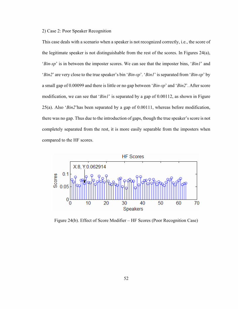
52
2) Case 2: Poor Speaker Recognition
This case deals with a scenario when a speaker is not recognized correctly, i.e., the score of
the legitimate speaker is not distinguishable from the rest of the scores. In Figures 24(a),
‘Bin-sp’ is in between the imposter scores. We can see that the imposter bins, ‘Bin1’ and
‘Bin2’ are very close to the true speaker’s bin ‘Bin-sp’. ‘Bin1’ is separated from ‘Bin-sp’ by
a small gap of 0.00099 and there is little or no gap between ‘Bin-sp’ and ‘Bin2’. After score
modification, we can see that ‘Bin1’ is separated by a gap of 0.00112, as shown in Figure
25(a). Also ‘Bin2’has been separated by a gap of 0.00111, whereas before modification,
there was no gap. Thus due to the introduction of gaps, though the true speaker’s score is not
completely separated from the rest, it is more easily separable from the imposters when
compared to the HF scores.
Figure 24(b). Effect of Score Modifier – HF Scores (Poor Recognition Case)

53
Figure 25(a). Effect of Score Modifier – HFA Score Histogram (Poor Recognition Case)
Figure 25(b). Effect of Score Modifier – HFA Scores (Poor Recognition Case)
3) Case 3: Poor Accent Classification
This case deals with a scenario where a speaker was recognized correctly, but the true
speaker’s accent was not identified correctly. In Figure 26(a), ‘Bin-sp’ is clearly separated
from the imposter bins. We can see that the imposter bin ‘Bin2’ is separated from ‘Bin-sp’ by
a gap of 0.00319. After score modification, we can see that the score of the true speaker has
been modified from 0.028761 to -0.056982, as shown in Figure 27(a). This indicates an
accent classification error because the score modifier modifies any score which does not
belong to the trained accent as that of the true speaker. Because of this subtraction, even

54
when there is an error in accent classification, the speaker’s score that was truly recognized
is further improved but not degraded. Degradation might occur only with a completely
inseparable true speaker score and an error in accent classification.
Figure 26(a). Effect of Score Modifier – HF Score Histogram (Poor Accent Classification Case)
Figure 26(b). Effect of Score Modifier – HF Scores (Poor Accent Classification Case)

55
Figure 27(a). Effect of Score Modifier – HFA Score Histogram (Poor Accent Classification Case)
.
Figure 27(b). Effect of Score Modifier – HFA Scores (Poor Accent Classification Case)

56
CHAPTER 5
EXPERIMENTAL RESULTS
The HF system, accent classification system and the HFA system have been evaluated on
various datasets; the results of these experiments are provided in this Chapter. The HF
speaker recognition system has been evaluated on YOHO [41] and the USF multi-modal
biometric dataset [8]. For evaluating accent incorporation, i.e. accent classification system
and HFA system, SAA system and the USF multi-modal biometric dataset were used. The
YOHO dataset was not used for evaluating accent incorporation, as the dataset comprised of
only North American accents.
5.1 Datasets
1) YOHO Dataset
YOHO dataset, which can be obtained from Linguistic Data Consortium (LDC), was created
in a low noise office environment and has a population of 138 persons (106 males and 32
females). Data structure contains two different types of data-training and testing. Each
speaker reads a portion of a six digit combination lock phrases. There are 4 enrollment
sessions of 24 utterances. For verification, there are 10 verification session with 4 utterances.

57
Speaker’s voice was recorded using a telephone handset (Shure XTH-383). Data sampling
rate is 8000 Hz. Data set was collected over a three month period [11]. YOHO dataset was
designed to ascertain system accuracy up to 0.1% false rejection and 0.01% false acceptance
rate with 75% confidence.
2) USF Multi-Modal Biometric Dataset
A multi-modal biometric dataset was collected at USF over a time period of nine months. In
this dataset 78 persons provided three sessions of indoor and outdoor data for face, voice and
fingerprint. As we have used only the voice dataset in this work, we will describe only that
portion of the dataset. Each person’s voice samples were acquired using Sennheiser E850
microphone in collecting both indoor and outdoor datasets. There are three sets of phrases in
the voice dataset: Fixed:-one fixed sentence was uttered by every person; Semi-fixed:-
sentence was varied by a small amount for each speaker, i.e., date and time of recording;
Random:-completely random utterance. Each person uttered three types of phrases and each
phrase was repeated three times, for both indoor and outdoor locations. This gives 9 voice
samples for indoor and outdoor per person per session. Sampling rate was 11,025 Hz. There
are three different sessions of data available in this dataset. Not all volunteers showed up for
all the sessions. Therefore, we used two sessions of data, with population of 65 people. We
used indoor data as training and outdoor data for testing.
3) SAA Dataset
The SAA dataset [42], is an online speech database, available to people who wish to
compare and analyze different accents of the English language. The archive provides a large
set of speech samples from a variety of language backgrounds. All data has been sampled at

58
22,050 Hz. All the speakers read the following paragraph. “Please call Stella. Ask her to
bring these things with her from the store: Six spoons of fresh snow peas, five thick slabs of
blue cheese, and maybe a snack for her brother Bob. We also need a small plastic snake and
a big toy frog for the kids. She can scoop these things into three red bags, and we will go
meet her Wednesday at the train station.”
For our purpose, we have selected six accents in order to classify the speakers which
are Arabic, American, Indian, Chinese, Russian, and Spanish. Though all subjects were
recorded in a quiet room environment, the pool used for this purpose had background noise
in some cases and an echo in some other cases. In order to test the SAA dataset itself, the
phrase “Please call Stella” was used for training the accent model and “Six spoons of fresh
snow peas” was used for testing purposes. 10 speakers per accent were used to train each
accent model. For testing the USF dataset, these training models were used as a reference
accent database. The performance results of the systems are shown next, starting with hybrid
fusion system performance.
5.2 Hybrid Fusion Performance
A frame size of 256 samples per window was used for YOHO and USF datasets. A
Hamming window was applied and the FFT size used was 256 points. From each speech
signal, 13 MFCCs (mel- frequency cepstral coefficients) for both datasets was extracted at
every 256 samples of window (approximately 32 ms for YOHO and 25 ms for USF dataset)
with overlap of 128 samples (approximately 16 ms for YOHO and 10 ms for USF dataset).
Each HMM was represented using 30 hidden states with 200 iterations for each enrolled or

59
training speech data sample. Once HMM models were created as described in Section 2.4.2,
they were compared with the testing data to find the likelihood score. AHS distance measure
(score matrix) from training and testing speech data was found as described in Section 2.4.1.
Figure 28(a). ROC Comparisons of AHS, HMM, and HF systems for YOHO Dataset
These scores were normalized using Min-Max normalization technique as described
in Section 2.5.1 so that the scores are between [0, 1]. Lower score represents closer
likelihood between training and testing subjects. The fusion method described in Section
2.5.2 was used to determine the mean of AHS and HMM distributions MHMM and MAHS,
respectively. Once the enhanced weightω was found algorithmically using Equation (34),
we fuse both the score metrics to obtain an enhanced score metric.

60
Figure 28(b). ROC Comparisons of AHS, HMM, and HF Systems for USF Dataset
In order to represent the score matrices, the Receiver Operating Characteristic (ROC)
curve, which is a plot of the False Acceptance Rate (FAR) versus the True Acceptance Rate
(TAR) of the system, was used. Figures 28(a), (b) and (c), show the ROC curve for each of
the recognition methods, i.e., AHS, HMM and HF conducted on YOHO, USF, and SAA
datasets, respectively. It can be seen that on all the datasets our HF method shows an
improvement. However, the improvement was better for fusion on YOHO and SAA dataset
(Figures 28(a), 28(c)) compared to USF dataset (Figure 28(b)).

61
Figure 28(c). ROC Comparisons of AHS, HMM, and HF Systems for SAA Dataset
For better appreciation of the performance gains from hybrid fusion method, Figures 28(a),
(b) and (c) are expressed in a bar graph in Figures 29, 30 and 31, respectively. It can be seen
that the proposed HF method works better when the dataset (YOHO) was noise free. For
YOHO dataset, the TAR performances were 84% and 62% at 5% FAR for HF and AHS
methods, respectively. A 22% performance increase, when compared to AHS, which
performed better than HMM at 5% FAR (55% TAR). Therefore it would be prudent to
compare the performance gain with the better performing algorithm. The HMM method was
not speaker adapted, thus the accuracy is lower than HMM in conjunction with maximum a
posteriori probability (MAP) algorithm’s performance [26]. YOHO dataset can provide

62
enough training samples for MAP algorithm to be effective, however USF dataset does not
have enough training samples (per session) to create speaker adaptation.
Enhanced Recognition at various FARs (YOHO)
0
10
20
30
40
50
60
70
80
90
3 5False Acceptance Rate (%)
True
Acc
epta
nce
Rat
e(%
)
AHS
HMM
HF
Figure 29. Comparison of AHS, HMM, and HF Recognition Rate at Various False
Acceptance Rates for YOHO Dataset
For USF outdoor dataset, the TAR performances were 71% and 65% at 5% FAR for HF and
AHS/HMM methods, respectively. A 6% increase in performance at 5% FAR. For this noisy
dataset, performance increase was not as drastic as the cleaner YOHO dataset. From Figures
29, it can be seen that HF method shows about 22% increase in YOHO dataset at 3% FAR.
However from Figure 30, it can be seen that HF method does not show such improvement
when used with USF dataset. TARs were 63% and 59% at 3% FAR for HF and HMM (4%
performance gain for HF over HMM). For SAA dataset (Figure 31), the TAR performances
were 71% and 50% at 3% FAR for HF and HMM, respectively (21% performance gain). But

63
at 5%, a TAR of 74% and 65% for HF and HMM systems can be observed, resulting in a 9%
performance increase.
Enhanced Recognition at Various FARs (USF data)
0
10
20
30
40
50
60
70
80
3 5False Acceptance Rate (%)
True
Acc
epta
nce
Rat
e (%
))
AHS
HMM
HF
Figure 30. Comparison of AHS, HMM, and HF Recognition Rate at Various False
Acceptance Rates for USF Dataset
It is always difficult for any recognition system to perform well when an outdoor
dataset is used. USF location being in a large metropolitan city of Tampa combined with a
typical busy campus environment resulted in our outdoor speech dataset to be noisy and
unpredictable. This explains the lower performance for both AHS and HMM systems when
compared to noise free YOHO dataset and the SAA dataset. Thus after fusion, we do not see
much performance gain (6% at 5% FAR and 4% at 3% FAR).

64
Enhanced Recognition at Various FARs (SAA data)
0
10
20
30
40
50
60
70
80
3 5False Acceptance Rate (%)
True
Acc
epta
nce
Rat
e (%
))
AHS
HMM
HF
Figure 31. Comparison of AHS, HMM, and HF Recognition Rate at Various False
Acceptance Rates for SAA Dataset
We could not compare our results, with FAR less than 2 to 3% for the USF dataset
reliably, because the population size was only 65. In other words one erroneous result could
swing the performance, by ±1.5%. For the same reason, having a smaller number of speakers
in a dataset, with a performance increase (1% or less), as reported in [26], would not be
statistically viable.
From Figures 29-31, we can see that AHS and HMM show similar performance
varying around 50-65% for all the datasets at 3 to 5% FAR. Yet we see HF method resulted
in enhanced performances. In our case HF assigns a larger weight to HMM and a relatively
much smaller weight to AHS. Even though AHS and HMM are analogous in performance,
mean enhanced weight method makes HF outperform individual algorithm’s TAR. The

65
reason behind the success of such weight assignment is the utilization of the means of the
score distribution, rather than the score distribution itself.
5.3 Accent Classification Performance
The sampling rate of SAA and USF dataset being different, we used fixed window period of
25.6 ms with 50% overlap for both datasets. A Hamming window was applied and the FFT
size used was 256 points. We extracted 13 MFCCs, 13 ASCCs, 13 delta ASCCs, delta-delta
Energy, delta Energy and Energy from each speech signal as described in Section 3.4 from
both datasets.
For each enrolled or training SAA speech data sample we used 6 hidden states and 8
Gaussians each with a diagonal covariance and 100 iterations to represent a CHMM as
explained in Section 3.5.2. GMMs were created using 7 components with diagonal
covariances as explained in Section 3.5.1. The SAA testing data was modeled using 6 states
and 15 Gaussians for CHMM and 15 components for GMM. On the other hand the USF
dataset was modeled by using 6 states and 18 Gaussians for CHMM and 16-component
GMM. Once CHMMs and GMMs were created they were fused according to Equation (49).
Then, the accent scores and accent classes for each enrolled and test speakers are stored.
After which the SM algorithm of Section 4.1 is used to enhance the HF score matrix. In the
case of testing the SAA dataset, the enrolled speakers were already labeled; hence the accent
classification system was applied only to the test speakers. In case of USF dataset, both the
enrolled and test speakers were classified using the accent classification system with the
SAA dataset as a reference.

66
The weight factor β in Equation (52) was used to tune the fusion of CHMM and
GMM accent scores. As Figure 32 shows, best results were obtained for β = 0.95, 0.75 for
SAA and USF datasets respectively. The graph indicates that as the weight factor is changed
from 0 to 1, i.e., GMM alone is used when β is 0, whereas CHMM is used when it is 1.
There was an improvement of 7% for SAA and 5% for USF datasets, due to fusion of GMM
and CHMM, instead of using GMM alone. Hence the final accent classification rate is 90%
and 57% for SAA and USF datasets, respectively.
Figure 32. Accent Classification Rate Using Different Weight Factors for SAA and USF
Datasets

67
5.4 Hybrid Fusion - Accent Performance
It can be seen from Figures 33(a) and 33(b) that for both datasets our HF method shows an
improvement. However, the improvement was better for fusion on SAA dataset (Figure
33(a)) compared to USF dataset (Figure 33(b)), because of high accent classification rate.
Intuitively, accent classification rate in SAA should be better because the reference accent
models were created from the same SAA dataset. These final results were obtained by
selecting a CAM value of 30 and 52 for USF and SAA datasets respectively. Also, the accent
classification rate of SAA was 1.6 times greater than that of USF dataset, interestingly the
same rule applies for the CAM variable as well.
Figure 33(a). ROC Comparisons for HF and HFA Methods Evaluated on SAA

68
For better appreciation of the performance gains from Hybrid Fusion – Accent (HFA)
method, Figures 33(a) and (b) are expressed in a bar graph in Figures 34 and 35,
respectively. For SAA dataset, the TAR performances were 88% and 71% at 3% FAR for
HFA and HF methods, respectively, i.e., a 17% performance gain for HFA method over HF
method.
For USF outdoor dataset, the TAR performances were 78% and 63% at 3% FAR for
HFA and HF methods, respectively. A 15% increase in performance has been achieved for
HFA method compared to HF method. From Figures 34 and 35, it can be seen that HFA
method shows about 20% increase in SAA dataset at 5% FAR. Also, it can be seen that HFA
method shows significant improvement when used with the noisy outdoor USF dataset. At
5% FAR, a 13% performance increase was observed for HFA method compared to HF
method. We can see from Figure 33(b), that at very high FARs, HFA method does not
perform better than HF method. When speaker recognition performs poorly, a higher score is
assigned to the true speaker, due to which the true speaker’s score lies within the false
speaker cluster. But when SM algorithm is applied to the HF-score matrix, it modifies the
imposter scores making those false scores come closer towards the true speaker’s score,
thereby decreasing the TAR at higher FARs. Since FARs as high as 10% are never useful in
evaluating a real world speaker recognition system, this specific issue is not a concern.
It is always difficult for any recognition system to perform well when an outdoor
dataset like USF dataset is used. But, incorporation of accent modeling brought a significant
performance gain at low FARs. A speaker recognition system cannot be considered as a
better performing system, even though it performs well at high FARs. A good system is

69
always expected to deliver performance at low FARs. We can see from Figures 34 and 35
that by adding accent information using SM algorithm, significant enhancement has been
achieved at low FARs. The accent incorporation method can be applied to any general
speaker recognition system with some adjustments to the weight factor β in the accent
classification system, distance threshold variable maxvar and CAM in the SM algorithm.
Figure 33(b). ROC Comparisons for HF and HFA Methods Evaluated on USF Dataset
Typically in any well performing speaker recognition system, the true speaker’s score would
be separated from most of the imposter scores, but still poorly separated from some of them.
Incorporation of accent modeling through the SM algorithm would especially achieve
significant performance gains in such scenarios. The SM algorithm increases the distance

70
between the true speaker and the some of the closely lying false speakers as well as the
distant imposters, resulting in two separate clusters where one cluster represents imposters
and the other cluster representing the rest, while the true speaker score stands separate from
either of them.
Enhanced Recognition at Various FARs (SAA)
0102030405060708090
100
3 5False Acceptance Rate (%)
True
Acc
epta
nce
Rat
e (%
)
HF HFA
Figure 34. Comparison of HFA and HF Recognition Rate at Various False Acceptance
Rates for SAA Dataset
On the whole, by implementing the HFA system, for SAA dataset, at 3% FAR, a
total recognition rate enhancement of 45% had been obtained through HFA. For USF
outdoor dataset, at 3% FAR, a 19% increase through HFA has been achieved.

71
Enhanced Recognition at various FARs (USF)
0
10
20
30
40
50
60
70
80
90
3 5False Acceptance Rate (%)
True
Acc
epta
nce
Rat
e (%
)
HF HFA
Figure 35. Comparison of HFA and HF Recognition Rate at Various False Acceptance
Rates for USF Dataset

72
CHAPTER 6
CONCLUSIONS AND FUTURE WORK
6.1 Conclusions
A good biometric system needs to deliver a high performance at low FARs. By using a text-
independent accent classification system with our HF system and a score modifier algorithm,
a significant enhancement has been achieved at low FARs. In this thesis, speaker recognition
using Arithmetic Harmonic Sphericity (AHS) and Hidden Markov Model (HMM) has been
studied. Mel-frequency cepstral coefficients (MFCC) have been used as speaker features. A
linear weighted fusion method (hybrid fusion), has been implemented effectively such that
the contrastive nature of AHS and HMM is used to benefit the speaker recognition
performance.
For the first time a text-independent accent classification (AC) system has been
developed without the usage of an automatic speech recognizer. MFCCs, accent sensitive
cepstral coefficients (ASCCs) and energy have been used as accent features. MFCCs
emphasize the first formant frequency, whereas ASCCs emphasize second and third
formants. By combining MFCCs and ASCCs along with energy increases accent
classification rate. Gaussian mixture model (GMM) and continuous hidden Markov model
(CHMM) have been used to model these features. Continuous HMM was used instead of
discrete HMM, as each state in CHMM is modeled as a mixture of Gaussians thereby
73
increasing precision and decreasing degradation. As GMM and CHMM were fused to benefit
from the advantages of both the modeling algorithms, an increase in accent classification
performance was observed. Then, the HF-speaker recognition system was combined with
accent classification system to enhance the true acceptance rate (TAR) at lower false
acceptance rates (FAR). The AC system produces accent class information and the accent
score assigned to each speaker. A score modifier algorithm was introduced, to incorporate
the outputs of the AC system into the HF-speaker recognition system. The score modifier
enhances the speaker recognition, even for low accent classification rates, as it modifies the
HF-speaker recognition score as a factor of the confidence measure of the accent score and
the HF score. But SM algorithm might fail, when a very poor speaker system is paired with a
poor accent classification system. Although there have been previous efforts in using accent
to improve speaker recognition, utilizing an accent classification system to enhance a
speaker recognition has not been reported so far.
The HF system was evaluated on the YOHO clean speech dataset and the realistic
outdoor USF dataset. But the enhancement achieved with HF for the USF dataset was not
sufficient, due to which an accent incorporation method was developed to achieve substantial
performance levels at lower FARs. The final accent incorporated HF model called the hybrid
fusion - accent (HFA) system was evaluated on SAA dataset and USF dataset. Significant
improvement was observed by using the HFA system. For SAA dataset, at 3% FAR, a total
recognition rate enhancement of 45% had been obtained through HFA. For USF outdoor
dataset, at 3% FAR, a 19% increase through HFA has been achieved. Finally, accent
incorporation and hybrid fusion technique can be applied to any general speaker recognition

74
system with some adjustments to the weight factor in the accent classification system,
distance threshold variable maxvar and CAM in the SM algorithm. Even though
performance gains has been achieved at lower FARs using the HFA system, further
improvements are necessary before the proposed speaker recognition system can be
considered as a stand alone security system.
6.2 Recommendations for Future Research
The HFA system still needs to be tuned for different datasets, i.e. the weight factor in the
accent classification system and the distance threshold variable maxvar, CAM in the score
modifier algorithm. Complete automation of the accent classification system and the score
modifier, would be useful, so that no tuning needs to be done for different datasets. Higher
level features other than mel-frequency cepstral coefficients (MFCC), accent-sensitive
cepstral coefficients (ASCC), delta ASCCs, energy, delta energy and delta delta energy
needs to be integrated into the system, so that an accent classification rate can be improved,
which would enhance the HFA system performance inturn. The HFA system needs to be
evaluated on a variety of larger datasets, so that more inferences can be drawn from the
results and enhancements to the HFA can be made. Also different fusion techniques at the
modeling level such as SVM versus GMM, HMM versus SVM needs to be studied, and
evaluated on a variety of datasets to better understand the effect of different fusions, so that a
common frame work can be formulated to find the optimal fusion. Finally, as we know from
the results that accent incorporation enhances speaker recognition, studies have to be
conducted on several other factors such as gender classification systems.

75
The process of identifying human through speech is a complex one and our own
human recognition system is an excellent instrument to understand this process. The human
recognition system extracts several other features from a single speech signal, due to which it
achieves high accuracy. The goal of a speech researcher should be to identify such missing
pieces of information, in a hope to match the human recognition system some day.

76
REFERENCES
[1] “Homeland Security Advisory System,” [online] Available:
http://www.dhs.gov/xinfoshare/programs/Copy_of_press_release_0046.shtm. [2] “Msnbc,” [online] Available: http://www.msnbc.msn.com/id/3078480/. [3] D. A. Reynolds, “Automatic Speaker Recognition: Current Approaches and
Future Trends,” Speaker Verification: From Research to Reality, 2001. [4] S. Furui, “Fifty Years of Progress in Speech and Speaker Recognition,” Journal
of Acoustical Society of America, vol. 116, no. 4, pp. 2497-2498, May 2004. [5] T. Mansfield, G. Kelly, D. Chandler, and J. Kane, “Biometric Product Testing
Final Report,” CESG/BWG Biometric Test Programme, no. 1, March 2001. [6] J. Kittler, M. Hatef, R. P. Duin, and J. G. Matas, “On Combining Classifiers,”
IEEE Trans. Pattern Analysis and Machine Intelligence, vol. 20, no. 3, pp. 226-239, March 1998.
[7] A. K. Jain, K. Nandakumar, and A. Ross, “Score Normalization in Multimodal
Biometric Systems,” Pattern Recognition, vol. 38, pp. 2270-2258, December 2005.
[8] H. Vajaria, T. Islam, P. Mohanty, S. Sarkar, R. Sankar, and R. Kasturi,
“Evaluation and Analysis of a Face and Voice Outdoor Multi-Biometric System,” Pattern Recognition Letters, vol. 28, no. 12, pp. 1572-1580, September 2007.
[9] T. Islam, S. Mangayyagari, and R. Sankar, “Enhanced Speaker Recognition
Based on Score-Level Fusion of Ahs and Hmm,” IEEE Proc. SoutheastCon, pp. 14-19, 2007.
[10] F. Bimbot and L. Mathan, “Text-Free Speaker Recognition Using an Arithmetic-
Harmonic Sphericity Measure,” Third European Conference on Speech Communication and Technology, 1993.
[11] L. E. Baum and T. Petrie, “Statistical Inference for Probabilistic Functions of
Finite State Markov Chains,” The Annals of Mathematical Statistics, vol. 37, no. 6, pp. 1554-1563, 1966.

77
[12] D. A. Reynolds and R. C. Rose, “Robust Text-Independent Speaker Identification Using Gaussian Mixture Speaker Models,” IEEE Trans. Speech and Audio Proc., vol. 3, no. 1, pp. 72-83, January 1995.
[13] B. H. Juang, S. E. Levinson, and M. M. Sondhi, “Maximum Likelihood
Estimation for Multivariate Mixture Observations of Markov Chains,” IEEE Trans. Inform. Theory, vol. 32, no. 2, pp. 307-309, March 1986.
[14] S. Pruzansky, “Pattern-Matching Procedure for Automatic Talker Recognition,”
Journal of Acoustical Society of America, vol. 35, pp. 354-358, 1963. [15] P. D. Bricker, R. Gnanadesikan, M. V. Mathews, S. Pruzansky, P. A. Tukey, K.
W. Wachter, and J. L. Warner, “Statistical Techniques for Talker Identification,” Journal of Acoustical Society of America, vol. 50, pp. 1427-1454, 1971.
[16] B. S. Atal, “Text-Independent Speaker Recognition,” Journal of Acoustical
Society of America, vol. 52, 1972. [17] J. M. Naik, L. P. Netsch, and G. R. Doddington, “Speaker Verification over Long
Distance Telephone Lines,” Proc. ICASSP, pp. 524-527, 1989. [18] H. Gish and M. Schmidt, “Text-Independent Speaker Identification,” IEEE Signal
Processing Magazine, vol. 11, no. 4, pp. 18-32, 1994. [19] T. Matsui and S. Furui, “Comparison of Text-Independent Speaker Recognition
Methods Using VQ-Distortion and Discrete/Continuous HMM's,” IEEE Trans. Speech and Audio Proc., vol. 2, no. 3, pp. 456-459, 1994.
[20] G. Doddington, “Speaker Recognition Based on Idiolectal Differences between
Speakers,” Proc. Eurospeech, vol. 4, pp. 2521-2524, 2001. [21] A. G. Adami and H. Hermansky, “Segmentation of Speech for Speaker and
Language Recognition,” Proc. Eurospeech, pp. 841-844, 2003. [22] D. A. Reynolds, W. Andrews, J. Campbell, J. Navratil, B. Peskin, A. Adami, Q.
Jin, D. Klusacek, J. Abramson, and R. Mihaescu, “The Supersid Project: Exploiting High-Level Information for High-Accuracy Speaker Recognition,” Proc. ICASSP, vol. 4, pp. 784-787, 2003.
[23] D. A. Reynolds, W. Campbell, T. T. Gleason, C. Quillen, D. Sturim, P. Torres-
Carrasquillo, and A. Adami, “The 2004 MIT Lincoln Laboratory Speaker Recognition System,” Proc. ICASSP, vol. 1, 2005.
[24] A. Park and T. J. Hazen, “ASR Dependent Techniques for Speaker
Identification,” Proc. of ICSLP, pp. 2521-2524, 2002.

78
[25] T. J. Hazen, D. A. Jones, A. Park, L. C. Kukolich, and D. A. Reynolds, “Integration of Speaker Recognition into Conversational Spoken Dialogue Systems,” Proc. Eurospeech, pp. 1961-1964, 2003.
[26] S. Nakagawa, W. Zhang, and M. Takahashi, “Text-Independent Speaker
Recognition by Combining Speaker-Specific GMM with Speaker Adapted Syllable-Based HMM,” Proc. ICASSP. vol. 1, 2004.
[27] F. Farahani, P. G. Georgiou, and S. S. Narayanan, “Speaker Identification Using
Supra-Segmental Pitch Pattern Dynamics,” Proc. ICASSP, vol. 1, 2004. [28] M. M. Tanabian, P. Tierney, and B. Z. Azami, “Automatic Speaker Recognition
with Formant Trajectory Tracking Using Cart and Neural Networks,” Canadian Conference on Electrical and Computer Engineering, pp. 1225-1228, 2005.
[29] J. R. Deller, J. H. L. Hansen, and J. G. Proakis, Discrete – Time Processing of
Speech Signals, NJ: IEEE Press, 2000. [30] L. M. Arslan, “Foreign Accent Classification in American English,” Ph. D.
Dissertation, NC: Duke University, 1996. [31] D. Crystal, A Dictionary of Linguistics and Phonetics, MA: Blackwell Publishing,
2003. [32] S. Gray and J. H. L. Hansen, “An Integrated Approach to the Detection and
Classification of Accents/Dialects for a Spoken Document Retrieval System,” IEEE Workshop on Automatic Speech Recognition and Understanding, pp. 72-77, 2005.
[33] L. W. Kat and P. Fung, “Fast Accent Identification and Accented Speech
Recognition,” Proc. ICASSP, vol. 1, 1999. [34] C. Teixeira, I. Trancoso, A. Serralheiro, and L. Inesc, “Accent Identification,”
Proc. of ICSLP, vol. 3, 1996. [35] T. Chen, C. Huang, E. Chang, and J. Wang, “Automatic Accent Identification
Using Gaussian Mixture Models,” IEEE Workshop on Automatic Speech Recognition and Understanding, pp. 343-346, 2001.
[36] X. Lin and S. Simske, “Phoneme-Less Hierarchical Accent Classification,”
Asilomar Conference on Signals, Systems and Computers, vol. 2, 2004. [37] K. Bartkova and D. Jouvet, “Using Multilingual Units for Improved Modeling of
Pronunciation Variants,” Proc. ICASSP, vol. 5, pp. 1037-1040, 2006.

79
[38] P. Angkititrakul and J. H. L. Hansen, “Advances in Phone-Based Modeling for Automatic Accent Classification,” IEEE Trans. Audio, Speech and Language Processing, vol. 14, no. 2, pp. 634-646, 2006.
[39] M. V. Chan, X. Feng, J. A. Heinen, and R. J. Niederjohn, “Classification of
Speech Accents with Neural Networks,” IEEE World Congress on Computational Intelligence, vol. 7, pp.4483-4486, July 1994.
[40] S. Deshpande, S. Chikkerur, and V. Govindaraju, “Accent Classification in
Speech,” Fourth IEEE Workshop on Automatic Identification and Advanced Technologies, pp. 139-143, 2005.
[41] J. P. Campbell Jr., “Testing with the Yoho Cd-Rom Voice Verification Corpus,”
Proc. ICASSP, vol. 1, 1995. [42] Speech Accent Archive, George Mason University, [online] Available:
http://accent.gmu.edu.

80
APPENDICES

81
Appendix A: YOHO, USF, AND SAA DATASETS
TABLE 1. YOHO Dataset
Sampling Frequency 8 KHz
# of speakers 138 (106 M/32 F)
# of sessions/speaker 4 enrollments, 10 verifications
Intersession Interval Days-Month (3 days)
Type of speech Prompted digit phrases
Microphones Fixed, high quality, in handset
channels 3.8 KHz/clean
Acoustic Environment Office
Evaluation Procedure Yes [11]
Language American English
TABLE 2. USF Dataset
Sampling Frequency 11.025 kHz
# of speakers 78
# of sessions/speaker /utterance/Location 3 sessions
Period of time 9 months
Type of speech Fixed , Semi-Fixed and Random Phrases
Microphone Sennheiser E850
Acoustic Environment Indoor Office and Outdoor Campus
Language English

82
Appendix A: (Continued)
TABLE 3. SAA (subset) Dataset
Sampling Frequency 22.050 kHz
# of speakers 60
# of accents 6
accents Arabic, American, Indian, Chinese, Russian and Spanish
Type of speech Paragraph split into two phrases
Microphone Sony ECM-MS907
Acoustic Environment Indoor Office (but has non stationary noise)
Language English

83
Appendix B: WORLD’S MAJOR LANGUAGES
Figure 36. World’s Major Languages [30]