vol implied
TRANSCRIPT

Do Implied Volatilities Predict Stock Returns?
Manuel Ammann, Michael Verhofen and Stephan Suss∗
University of St. Gallen
Abstract
Using a complete sample of US equity options, we find a positive,
highly significant relation between stock returns and lagged implied
volatilities. The results are robust after controlling for a number of
factors such as firm size, market value, analyst recommendations and
different levels of implied volatility. Lagged historical volatility is - in
contrast to the corresponding implied volatility - not relevant for stock
returns. We find considerable time variation in the relation between
lagged implied volatility and stock returns.
Keywords: Implied Volatility, Expected Returns
JEL classification: G10
∗Manuel Ammann ([email protected]) is professor of finance at the University
of St. Gallen, Switzerland (Rosenbergstrasse 52, CH-9000 St. Gallen, Phone: +41 71 224
7000), Michael Verhofen ([email protected]) is portfolio manager at Allianz Global
Investors (Mainzer Landstrasse 11-13, D-60329 Frankfurt, Phone: +49 69 263 14394)
and lecturer in finance at the University of St. Gallen, Switzerland, and Stephan Suss
([email protected]) is research assistant at the University of St. Gallen, Switzerland
(Rosenbergstrasse 52, CH-9000 St. Gallen, Phone: +41 71 224 7000). We thank Sebastien
Betermier, Peter Feldhutter, Thomas Gilbert, Sara Holland, Peter Tind Larsen, Miguel
Palacios, Hari Phatak, David Skovmand and Ryan Stever for helpful comments.

1 Introduction
The option market reveals important information about investors’ expecta-
tions of the underlying’s return distribution. While considerable research
has examined the informational content of index options, little is known
about individual equity options. Using a complete sample of US equity op-
tions, we analyze the relation between implied volatility and future realized
returns.
In the last three decades, several articles have documented a small degree
of predictability in stock returns based on prior information, specifically at
long horizons. In the long run, dividend yields on an aggregate stock port-
folios predict returns with some success, as shown by Campbell & Shiller
(1988), Fama & French (1988, 1989), as well as Goyal & Welch (2003). Ad-
ditional variables found to have predictive power include the short-term in-
terest rate (Fama & Schwert (1977)), spreads between long- and short-term
interest rates (Campbell (1987)), stock market volatility (French, Schwert
& Stambaugh (1987)), book-to-market ratios (Kothari & Shanken (1997),
Pontiff & Schall (1998)), dividend-payout and price-earnings ratios (Lam-
ont (1998)), as well as measures related to analysts’ forecasts (Lee, Myers &
Swaminathan (1999)). Baker & Wurgler (2000) detect a negative relation-
ship between IPO activity and future excess returns. Lettau & Ludvigson
(2001) find evidence for predictability using a consumption wealth ratio.
Recently, the relation between historical volatility and stock returns has
been addressed by a number of authors (e.g., Goyal & Santa-Clara (2003),
Bali, Cakici, Yan & Zhang (2005), and Ang, Hodrick, Xing & Zhang (2006)).
Goyal & Santa-Clara (2003) analyze the predictability of stock market re-
turns with several risk measures. They find a significant positive relation
between the cross-sectional average stock variance and the return on the
market, whereas the variance of the market has no forecasting power for
the market return. However, Bali et al. (2005) disagree with these findings.
2

They argue that the results are primarily driven by small stocks traded
on the NASDAQ, and are therefore partially due to a liquidity premium.
Moreover, the results do not hold for an extended sample period. Ang et al.
(2006) examine the pricing of aggregate volatility risk in the cross-section
of stock returns. They find that stocks with high idiosyncratic volatility in
the Fama and French three-factor model have very low average returns.
Option-implied volatility is different from most of the variables used for
predicting stock returns in at least two respects. First, it is a real forward-
looking variable measuring market participants’ expectations. Second, it is
a traded price and therefore less likely to be affected by biases.
To our best knowledge, no study exists that systematically analyzes the
informational content of implied volatility in the cross-section. Existing
studies have only focussed on index option data or a very small sample of
single equity options. This study contributes to the existing literature by
investigating the relation between implied volatility and stock returns on a
very large data basis.
To analyze the relation between implied volatility and stock returns, we ap-
ply a predictive regression approach in univariate and multivariate settings.
Our results are based on the OptionMetrics database, which contains a sur-
vivial bias-free, complete data set of implied volatilities for the US stock
market. To control for a number of factors and to investigate the stability
of the findings, we merge our sample with the CRSP, Compustat, and IBES
FirstCall data. Model misspecification is addressed by using different regres-
sion settings. We address parameter uncertainty by a bootstrapping and an
additional rolling-windows approach.
We find a highly significant, positive relation between returns and lagged
implied volatilities. This dependence is stronger for firms with small market
capitalizations and is independent of different valuation levels, measured by
the book-to-market ratio. Our findings are persistent after controlling for
3

market risk (using the CAPM) and the exposure to the risk factors in the
Carhart four-factor model. The informational content of first-order diffe-
rences of implied volatility seems to be limited. With respect to analyst re-
commendations, we find weaker relations between returns and lagged implied
volatilities for companies with higher analyst coverages. The findings seem
to be stable for different times to maturity of implied volatility. Historical
volatilities do not seem to have the same informational content as implied
volatilities. We find considerable time variation in the relation between
lagged implied volatility and stock returns. The out-of-sample predictive
power is weak compared to the iid model.
The paper is organized as follows: Section 2 outlines our research design,
as well as the applied data set. Section 3 presents the empirical results.
Section 4 concludes.
2 Research Design
2.1 Data
To obtain the data set for our empirical analysis, we merge five different
databases. From OptionMetrics, we retrieve option price data and historical
volatilities. Equity return data are obtained from the CRSP database. The
book values and market capitalization figures are from Compustat. Analyst
forecasts are collected from IBES. The respective risk premia are from the
Fama and French database. Data are merged by the respective CUSIP
as identifier. Our sample with monthly frequency covers the period from
January 1996 to December 2005.
The OptionMetrics database is described in detail in Optionmetrics (2005).
Our study is based on implied volatility for standardized call options with a
maturity of 91 calendar days and a strike price equal to the forward price.
They are computed as outlined in Optionmetrics (2005). In addittion to
4
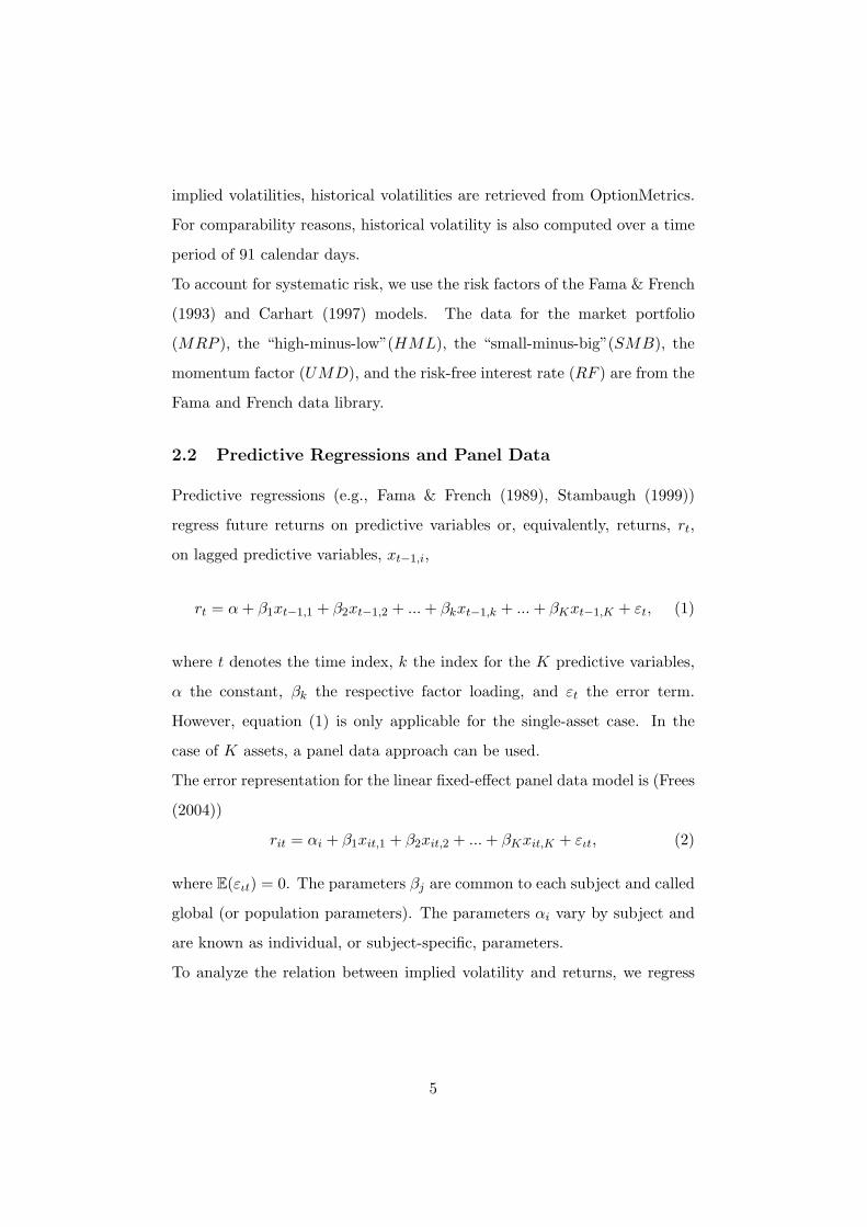
implied volatilities, historical volatilities are retrieved from OptionMetrics.
For comparability reasons, historical volatility is also computed over a time
period of 91 calendar days.
To account for systematic risk, we use the risk factors of the Fama & French
(1993) and Carhart (1997) models. The data for the market portfolio
(MRP ), the “high-minus-low”(HML), the “small-minus-big”(SMB), the
momentum factor (UMD), and the risk-free interest rate (RF ) are from the
Fama and French data library.
2.2 Predictive Regressions and Panel Data
Predictive regressions (e.g., Fama & French (1989), Stambaugh (1999))
regress future returns on predictive variables or, equivalently, returns, rt,
on lagged predictive variables, xt−1,i,
rt = α + β1xt−1,1 + β2xt−1,2 + ... + βkxt−1,k + ... + βKxt−1,K + εt, (1)
where t denotes the time index, k the index for the K predictive variables,
α the constant, βk the respective factor loading, and εt the error term.
However, equation (1) is only applicable for the single-asset case. In the
case of K assets, a panel data approach can be used.
The error representation for the linear fixed-effect panel data model is (Frees
(2004))
rit = αi + β1xit,1 + β2xit,2 + ... + βKxit,K + ειt, (2)
where E(ειt) = 0. The parameters βj are common to each subject and called
global (or population parameters). The parameters αi vary by subject and
are known as individual, or subject-specific, parameters.
To analyze the relation between implied volatility and returns, we regress
5

returns on lagged implied volatilities, V,
rit = αi + β1Vit−1,1 + ειt . (3)
The estimated factor loading β1 therefore summarizes the full sample rela-
tion between implied volatility and future stock returns.
2.3 Excess Returns
Besides raw returns, we use the CAPM and the Carhart (1997) four-factor
model to account for systematic risk effects. To estimate the exposure to-
wards the Fama & French (1993) risk factors and the Carhart (1997) mo-
mentum factor, we run the following regression for each asset i to control
for market, size, value, and momentum risk
rit − rft = αi,FF + βi,MRP ·MRPt + βi,HML ·HMLt +
βi,SMB · SMBt + βi,UMD · UMDt + εit (4)
and the following regression to control for market risk
rit − rft = αi,CAPM + βi,MRP ·MRPt + εit . (5)
2.4 Robustness
To analyze the robustness of our findings, we perform a number of different
analyses. First, we run the respective regressions for various subsamples.
Second, we use a rolling-window approach to account for time-varying factor
loadings. Third, we implement a bootstrapping approach to investigate
possible problem with the estimated used. Finally, we analyze the out-of-
sample performance.
To analyze the out-of-sample validity of the models we regress the realiza-
tions of each return rit on the corresponding time-t−1 return forecast rit−1,
6

i.e.,
rit = α + β · rit,t−1 + ειt. (6)
Under accurate forecasts, we expect α = 0 and β = 1.
3 Empirical Results
3.1 Regressions of Returns on Lagged Implied Volatility
Table 1 shows the basic results of this paper. In the first column, we show
the estimated factor loadings from a regression of returns on lagged implied
volatility. An estimated factor loading of 2.021 indicates that a 1% higher
implied volatility leads, on average, to a return increase of 2.021% in the
subsequent month. This finding is highly significant with a t-value of 9.457.
The goodness-of-fit of this model, measured by R2, is 0.8%.
The second column illustrates the estimated factor loading from a simple iid
model. Under the assumption of no predictability in returns, the best fore-
cast is a constant. The root-mean-squared-error (RMSE) of the iid model
is 16.8408. This value is only marginally higher than the RMSE value of
16.8379 for the model with implied volatility. Since these two values are
very similar, the findings suggest that the degree of predictability is low
even though the estimated factor loadings are highly significant.
To test for nonlinearity, we include the squared implied volatility in the
regression equation. The results in the third column show that the esti-
mated coefficient is insignificant with a value of 0.076. This suggests the
appropriateness of the linear model.
To account for time-varying means and dispersion of implied volatility, we
compute standardized z-scores. The regression of returns on standardized,
lagged implied volatility validates previous findings. With an estimated
coefficient of 0.939, we find a highly significant, positive relation between
implied volatility and future returns with a factor loading of 0.032.
7

To account for time-varying means and dispersion in stocks returns, we
also compute standardized z-scores for every month for the return data. A
regression of standardized returns on standardized, lagged implied volatility
reveals, as before, a positive and significant relation between risk and return.
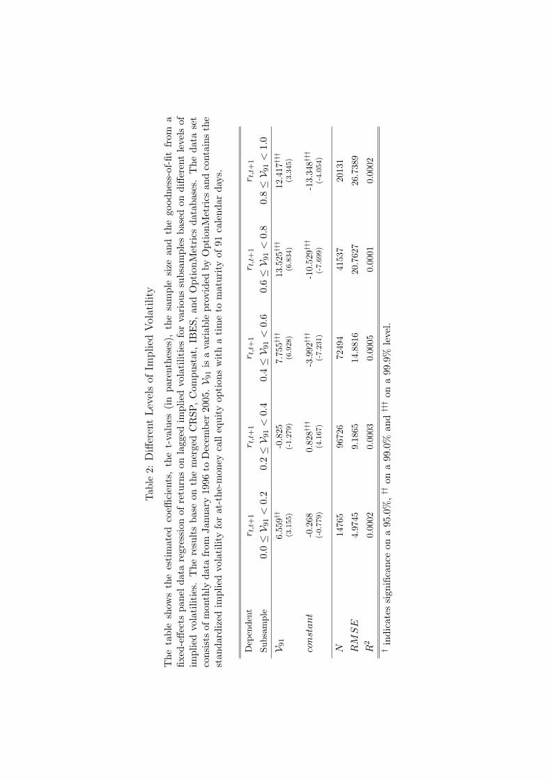
To analyze the robustness of these findings, we perform a number of different
analyses. First, we investigate whether the relation between returns and
lagged implied volatility is also valid for different levels of implied volatility.
For example, stocks with high implied volatility might behave differently
than stocks with comparably lower implied volatility.
Table 2 shows the estimated factor loadings for different subsamples. We re-
estimate the forecasting model for stocks with an implied volatility between
0% and 20% (subsample 1), 20% and 40% (subsample 2), 40% and 60%
(subsample 3), 60% to 80% (subsample 4), and 80% to 100% (subsample 5).
We find a positive, highly significant relation between returns and lagged
implied volatilities for subsamples 1, 3, 4, and 5. The estimated factor
loadings are of comparable magnitude for subsamples 1 and 3 (6.559 and
7.755) and for subsamples 4 and 5 (13.525 and 12.417). However, the findings
for subsample 2 are different. The estimated factor loading with a value of
-0.825 is slightly negative, but insigniicant.
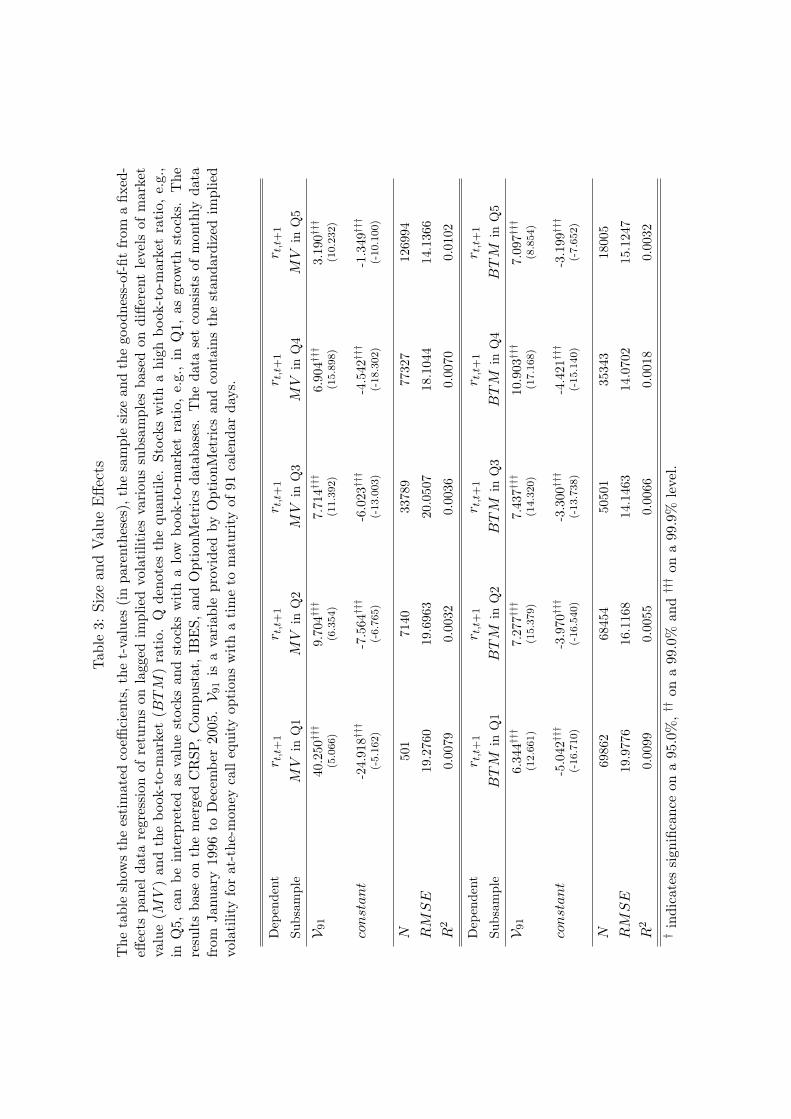
3.2 Size and Value Effects
Table 3 outlines the estimated factor loadings for separate regressions for
different quintiles of market capitalizations and book-to-market ratios.
With respect to market capitalization, we find that the strength of the re-
lation between anticipated risk and the subsequent return decreases with
higher market values. For stocks with the highest market capitalization
(Q5), we estimate a factor loading of 3.190 while the factor loading for small
stocks, e.g., in quantile 2 (Q2), is 9.704. All findings are highly significant.
The factor loading for growth stocks (Q1) is, with a value of 6.344, very
8

similar to the corresponding factor loading of value stocks (Q5), which has
a value of 7.097.
3.3 Excess Returns
Table 4 shows the results of the regression of excess returns on lagged implied
volatilities for the full sample and for various subsamples. In the upper part
of the table, excess returns have been computed against the CAPM model
and in the lower part against the Carhart four-factor model. Subsamples
are formed on different levels of implied volatility.
The estimated factor loadings are positive and highly significant for all sam-
ples. While the factor loading of implied volatility is 2.021 for raw re-
turns (see Table 1), it is higher when controlling for systematic risk fac-
tors. Against the CAPM, the coefficient is 7.772 for the full sample, against
the Carhart four-factor model, the corresponding coefficient has a value of
6.408. Both factor loadings are highly significant. We conclude that implied
volatility carries some information beyond that implied by the CAPM and
the Carhart four-factor model.
For subsamples formed on different levels of implied volatility, we find that,
in general, factor loadings increase with higher levels of implied volatility.
The subsample regressions validate the findings for the full sample.
3.4 First-Order Differences
Table 5 illustrates the estimated factor loadings of a regression of returns on
lagged, first-order differences of implied volatility. The first column shows
the results for the full sample, the remaining columns the respective results
of the regressions for various subsamples formed on the magnitude of first-
order differences of implied volatility.
With a value of 2.648 for the full sample, we find a highly significant, positive
relation between the returns and the lagged change in implied volatility.
9

Therefore, an investor can expect a higher monthly return for a stock if
implied volatility has increased in the previous month.
For subsamples formed on different directions and magnitudes of the change
in implied volatility, the results differ. First, we find hardly any significance
between the change in implied volatility and future returns. Second, the
estimated factor loadings differ substantially for different subsamples.
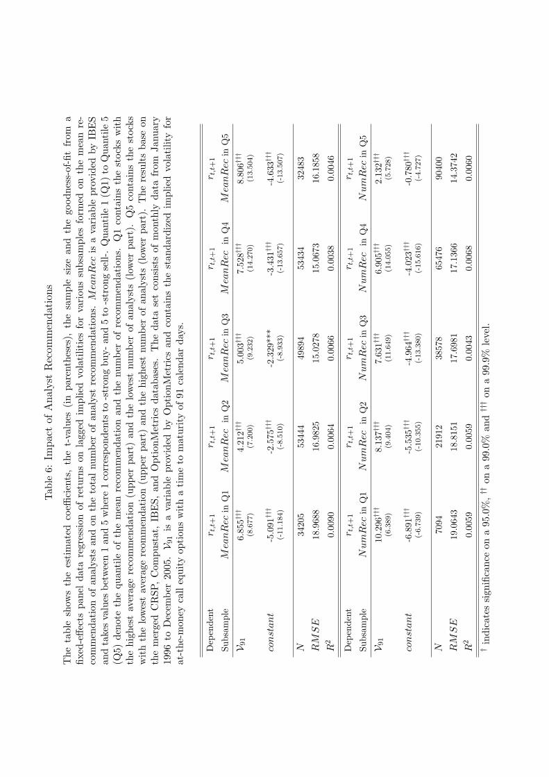
3.5 Analyst Forecasts
Table 6 shows the estimated factor loadings for subsamples formed on the
mean analyst recommendation. Quantile 1 contains the most favorable re-
commendations, Quantile 5 the least favorable recommendations. The ge-
neral observation, i.e., the positive relation between returns and lagged im-
plied volatility, holds for all subsamples based on different levels of analyst
recommendations. The findings are highly significant in all cases. The mag-
nitude of the relation between implied volatility and returns differs slightly
for different levels of analyst recommendations. For stocks with very positive
(Q1) or very negative recommendations (Q5), the estimated factor loadings
of 6.855 and 8.866, respectively, are higher than for stocks with an average
recommendation (Q3) where the value is 5.003.
Table 6 also shows the estimated regression coefficients for subsamples formed
on the number of analysts covering a specific stock. For all subsamples, the
relation between returns and lagged implied volatility is positive on a high
significance level. However, we find a monotonic decreasing relation be-
tween the estimated coefficients and the number of recommendations. The
higher the number of analysts following a particular stock, the lower the
informational content of implied volatility.
10

3.6 Implied Volatility vs. Historical Volatility
In Table 7, we outline the results of various regressions of returns on different
lagged variables. We analyze the dependence between returns and implied,
as well as historical volatilities with time horizons of 30, 60 and 91 days.
We find a very clear pattern. For all three different maturities of implied
volatilities, the estimated coefficients are highly significant and, with values
between 1.734 and 2.021, very similar. In contrast, we do not find a similar
pattern for historical volatility. The estimated coefficients are significant at
a 0.2% level for a time horizon of 30 days, and on a 5% level for a time
horizon of 91 days, but not for a time horizon of 60 days.
3.7 Univariate Regressions
Table 1 shows the histogram for the univariate regression of returns on
lagged implied volatility. The results should be interpreted carefully. Due
to the small sample size (monthly data for a maximum of 9 years), not
all coefficients are significant. Two main findings can be seen in Figure 2.
First, there is considerable cross-sectional dispersion in the factor loadings.
Second, the relation between implied volatility and return is, on average,
positive.
3.8 Parameter Uncertainty and Bootstrapping
Table 8 illustrates the estimated factor loadings of separate regressions for
each full year in the sample period, i.e. from 1996 to 2005. The estimated
factor loading of lagged implied volatility on return varies between 7.333
in 2003 and 33.482 in 2001. Therefore, there is always a positive, highly
significant relation between perceived risk and the subsequent return.
The goodness-of-fit varies substantially over time. In 2000 and 2001, the
model can explain more than 2% of total variance (2.20% and 2.33%). In
other years, e.g. 1996, 1999, and 2005, the R2 was very low, taking values
11

between 0.21% and 0.28%.
Figure 2 shows the estimated factor loading for a rolling window of 60 months
(5 years). Roughly speaking, the graph indicates an increase in the factor
loading from 4 to 11 from 2000 until 2002. In 2003, the factor loading
dropped to 3 and fluctuated between 2 and 6 until the end of the sample
period. Therefore, we find considerable time variation in the magnitude of
the relation between implied volatility and return. However, the estimated
factor loading is positive at any point in time.
Figure 3 shows the histogram of bootstrapped factor loadings for the full
sample regression and Figure 4 the associated t-values. As shown in Table 1,
the full-sample estimated coefficient is 2.021. Its corresponding t-value is
9.457. Both figures indicate that the findings are not spurious.
3.9 Out-of-Sample Performance
Table 9 gives the results from a predictive regression for the fixed effects
panel data model and the iid model. The parameters for both models are
estimated over a rolling horizon of 60 months. Based on the estimated
parameters, a return is predicted for the next month. The realized returns
are regressed on their corresponding predictions.
If forecasts are perfect, we expect a constant of 0 and slope coefficients of 1.
However, the empirical findings are quite different. For the one factor model
with implied volatility as predictive variable, the estimated constant is -1.169
and the slope coefficient has a value of -0.262. For a naive, iid model, the
estimated constant is also -1.169 and the slope coefficient is -0.293.
In its last row, Table 9 shows that the RMSE of the one-factor model is,
with a value of 17.373, higher than for the iid model with a value of 16.080.
12

4 Conclusion
To analyze the relation between implied volatility and stocks returns, we use
a predictive-regression approach in an univariate and multivariate setting.
We use the OptionMetrics database, which contains a survivial bias-free,
complete database for implied volatilities for the US stock market. A merge
of the database with CRSP, Compustat, and IBES FirstCall data allows
to control for a number of factors and to investigate the stability of the
findings. Model misspecification is evaluated by using different regression
settings. Parameter uncertainty is addressed by a bootstrapping approach
and a rolling windows approach. Furthermore, we consider the out-of-sample
validity.
As our main finding, we observe a highly significant, positive relation be-
tween returns and lagged implied volatilities. This relation is weaker for
larger market capitalizations and independent of different valuation levels
(using the book-to-market ratio). These findings are persistent after control-
ling for market risk (using the CAPM) and the risk factors of the Carhart
four-factor model. The informational content of first-order differences of
implied volatilities seems to be limited. With respect to analyst recom-
mendations, we find weaker relations between returns and lagged implied
volatilities for companies with high analyst coverages. A comparison of im-
plied volatilities for different time horizons shows that the patterns seem to
be stable for different time to maturities. Historical volatilities do not carry
the same informational content as implied volatilities. We find considerable
time variation in the relation between lagged implied volatility and stock
returns. The out-of-sample predictive power is weak compared to the iid
model.
13

References
Ang, A., Hodrick, R. J., Xing, Y. & Zhang, X. (2006), ‘The cross-section of
volatility and expected returns’, The Journal of Finance 61, 259.
Baker, M. & Wurgler, J. (2000), ‘The equity share in new issues and aggre-
gate stock returns’, Journal of Finance 55, 2219–2257.
Bali, T. G., Cakici, N., Yan, X. & Zhang, Z. (2005), ‘Does idiosyncratic risk
really matter?’, Journal of Finance 60, 905–929.
Campbell, J. (1987), ‘Stock returns and the term structure’, Journal of
Financial Economics 18, 373–399.
Campbell, J. & Shiller, R. (1988), ‘The dividend-price ratio and expectations
of future dividends and discount factors’, Review of Financial Studies
1, 195–227.
Carhart, M. (1997), ‘On persistence in mutual fund performance’, Journal
of Finance 52, 57–82.
Fama, E. & French, K. (1989), ‘Business conditions and expected returns
on stocks and bonds’, Journal of Financial Economics 19, 3–29.
Fama, E. & French, K. (1993), ‘Common risk factors in the returns on stocks
and bonds’, Journal of Financial Economics 33, 3–57.
Fama, E. & Schwert, G. (1977), ‘Asset returns and inflation’, Journal of
Financial Economics 5, 115–146.
Frees, E. W. (2004), Longitudinal and Panel Data, Cambridge University
Press, Cambridge.
French, K., Schwert, G. & Stambaugh, R. (1987), ‘Expected stock returns
and volatility’, Journal of Financial Economics 19, 293–305.
14

Goyal, A. & Santa-Clara, P. (2003), ‘Idiosyncratic risk matters!’, Journal of
Finance 58, 975–1007.
Goyal, A. & Welch, I. (2003), ‘Predicting the equity premium with dividend
ratios’, Management Science 49, 639–654.
Kothari, S. & Shanken, J. (1997), ‘Book-to-market, dividend yield, and
expected market returns: A time series analysis’, Journal of Financial
Economics 44, 169–203.
Lamont, O. (1998), ‘Earnings and expected returns’, Journal of Finance
53, 1563–1587.
Lee, C., Myers, J. & Swaminathan, B. (1999), ‘What is the intrinsic value
of the Dow’, Journal of Finance 54, 1639–1742.
Lettau, M. & Ludvigson, S. (2001), ‘Consumption, aggregate wealth, and
expected stock returns’, Journal of Finance 56, 815–849.
Optionmetrics (2005), ‘Ivy DB: File and data reference manual, version 2.5’.
Pontiff, J. & Schall, L. (1998), ‘Book-to-market as a predictor of market
returns’, Journal of Financial Economics 49, 141–160.
Stambaugh, R. (1999), ‘Predictive regressions’, Journal of Financial Eco-
nomics 54, 315–421.
15

Tab
le1:
Reg
ress
ions
ofR
eturn
son
Lag
ged
Implied
Vol
atility
Thi
sta
ble
illus
trat
esth
ees
tim
ated
coeffi
cien
ts,t-
valu
es(i
npa
rent
hese
s),sa
mpl
esi
zes,
root
-mea
n-sq
uare
d-er
rors
,as
wel
las
the
resp
ecti
veR
2fo
rfix
ed-e
ffect
spa
neld
ata
regr
essi
onof
retu
rns
onla
gged
impl
ied
vola
tilit
ies
for
the
full
sam
ple.
To
test
for
non-
linea
riti
es,w
eus
est
anda
rdiz
edan
dsq
uare
dim
plie
dvo
lati
litie
san
dre
turn
s.z(.
)de
note
sa
stan
dard
ized
vari
able
wit
hze
rom
ean
and
unit
vari
ance
.T
here
sult
sar
eba
sed
onth
em
erge
dC
RSP
,C
ompu
stat
,IB
ES,
and
Opt
ionM
etri
csda
taba
ses
wit
hm
onth
lyda
tafr
omJa
nuar
y19
96to
Dec
embe
r20
05.V 9
1is
ava
riab
lepr
ovid
edby
Opt
ionM
etri
csan
dco
ntai
nsth
est
anda
rdiz
edim
plie
dvo
lati
lity
for
at-t
he-m
oney
call
equi
tyop
tion
sw
ith
ati
me
tom
atur
ity
of91
cale
ndar
days
.
Dep
ende
ntr t
,t+
1r t
,t+
1r t
,t+
1r t
,t+
1z(r
t,t+
1)
Subs
ampl
eFu
llFu
llFu
llFu
llFu
ll
V 91
2.02
1†††
1.90
2†††
(9.4
57)
(3.9
53)
(V91)2
0.07
6(0
.277)
z(V
91)
0.93
9†††
0.03
2†††
(14.9
55)
(9.6
73)
(z(V
91))
2
const
ant
-1.4
74†††
-0.4
63†††
-1.4
38†††
-0.4
65†††
-0.0
00(-
13.1
70)
(-13.9
70)
(-8.4
66)
(-14.0
38)
(-0.0
04)
N25
8281
2582
8125
8281
2582
8125
8281
RM
SE
16.8
379
16.8
408
16.8
379
16.8
334
0.87
56
R2
0.00
800.
0000
0.00
800.
0055
0.00
61†
indi
cate
ssi
gnifi
canc
eon
a95
.0%
,††
ona
99.0
%an
d†††
ona
99.9
%le
vel.
Tab
le2:
Diff
eren
tLev
els
ofIm
plied
Vol
atility
The
tabl
esh
ows
the
esti
mat
edco
effici
ents
,th
et-
valu
es(i
npa
rent
hese
s),
the
sam
ple
size
and
the
good
ness
-of-fit
from
afix
ed-e
ffect
spa
nelda
tare
gres
sion
ofre
turn
son
lagg
edim
plie
dvo
lati
litie
sfo
rva
riou
ssu
bsam
ples
base
don
diffe
rent
leve
lsof
impl
ied
vola
tilit
ies.
The
resu
lts
base
onth
em
erge
dC
RSP
,C
ompu
stat
,IB
ES,
and
Opt
ionM
etri
csda
taba
ses.
The
data
set
cons
ists
ofm
onth
lyda
tafr
omJa
nuar
y19
96to
Dec
embe
r20
05.V 9
1is
ava
riab
lepr
ovid
edby
Opt
ionM
etri
csan
dco
ntai
nsth
est
anda
rdiz
edim
plie
dvo
lati
lity
for
at-t
he-m
oney
call
equi
tyop
tion
sw
ith
ati
me
tom
atur
ity
of91
cale
ndar
days
.
Dep
ende
ntr t
,t+
1r t
,t+
1r t
,t+
1r t
,t+
1r t
,t+
1
Subs
ampl
e0.
0≤V 9
1<
0.2
0.2≤V 9
1<
0.4
0.4≤V 9
1<
0.6
0.6≤V 9
1<
0.8
0.8≤V 9
1<
1.0
V 91
6.55
9††
-0.8
257.
755†††
13.5
25†††
12.4
17†††
(3.1
55)
(-1.2
79)
(6.9
28)
(6.8
34)
(3.3
45)
const
ant
-0.2
680.
828†††
-3.9
92†††
-10.
529†††
-13.
348†††
(-0.7
79)
(4.1
67)
(-7.2
31)
(-7.6
99)
(-4.0
54)
N14
765
9672
672
494
4153
720
131
RM
SE
4.97
459.
1865
14.8
816
20.7
627
26.7
389
R2
0.00
020.
0003
0.00
050.
0001
0.00
02†
indi
cate
ssi
gnifi
canc
eon
a95
.0%
,††
ona
99.0
%an
d†††
ona
99.9
%le
vel.
Tab
le3:
Siz
ean
dV
alue
Effec
ts
The
tabl
esh
ows
the
esti
mat
edco
effici
ents
,the
t-va
lues
(in
pare
nthe
ses)
,the
sam
ple
size
and
the
good
ness
-of-fit
from
afix
ed-
effec
tspa
nelda
tare
gres
sion
ofre
turn
son
lagg
edim
plie
dvo
lati
litie
sva
riou
ssu
bsam
ples
base
don
diffe
rent
leve
lsof
mar
ket
valu
e(M
V)
and
the
book
-to-
mar
ket
(BT
M)
rati
o.Q
deno
tes
the
quan
tile
.St
ocks
wit
ha
high
book
-to-
mar
ket
rati
o,e.
g.,
inQ
5,ca
nbe
inte
rpre
ted
asva
lue
stoc
ksan
dst
ocks
wit
ha
low
book
-to-
mar
ket
rati
o,e.
g.,
inQ
1,as
grow
thst
ocks
.T
here
sult
sba
seon
the
mer
ged
CR
SP,C
ompu
stat
,IB
ES,
and
Opt
ionM
etri
csda
taba
ses.
The
data
set
cons
ists
ofm
onth
lyda
tafr
omJa
nuar
y19
96to
Dec
embe
r20
05.V 9
1is
ava
riab
lepr
ovid
edby
Opt
ionM
etri
csan
dco
ntai
nsth
est
anda
rdiz
edim
plie
dvo
lati
lity
for
at-t
he-m
oney
call
equi
tyop
tion
sw
ith
ati
me
tom
atur
ity
of91
cale
ndar
days
.
Dep
ende
ntr t
,t+
1r t
,t+
1r t
,t+
1r t
,t+
1r t
,t+
1
Subs
ampl
eM
Vin
Q1
MV
inQ
2M
Vin
Q3
MV
inQ
4M
Vin
Q5
V 91
40.2
50†††
9.70
4†††
7.71
4†††
6.90
4†††
3.19
0†††
(5.0
66)
(6.3
54)
(11.3
92)
(15.8
98)
(10.2
32)
const
ant
-24.
918†††
-7.5
64†††
-6.0
23†††
-4.5
42†††
-1.3
49†††
(-5.1
62)
(-6.7
65)
(-13.0
03)
(-18.3
02)
(-10.1
00)
N50
171
4033
789
7732
712
6994
RM
SE
19.2
760
19.6
963
20.0
507
18.1
044
14.1
366
R2
0.00
790.
0032
0.00
360.
0070
0.01
02
Dep
ende
ntr t
,t+
1r t
,t+
1r t
,t+
1r t
,t+
1r t
,t+
1
Subs
ampl
eB
TM
inQ
1B
TM
inQ
2B
TM
inQ
3B
TM
inQ
4B
TM
inQ
5
V 91
6.34
4†††
7.27
7†††
7.43
7†††
10.9
03†††
7.09
7†††
(12.6
61)
(15.3
79)
(14.3
20)
(17.1
68)
(8.8
54)
const
ant
-5.0
42†††
-3.9
70†††
-3.3
00†††
-4.4
21†††
-3.1
99†††
(-16.7
10)
(-16.5
40)
(-13.7
38)
(-15.1
40)
(-7.6
52)
N69
862
6845
450
501
3534
318
005
RM
SE
19.9
776
16.1
168
14.1
463
14.0
702
15.1
247
R2
0.00
990.
0055
0.00
660.
0018
0.00
32†
indi
cate
ssi
gnifi
canc
eon
a95
.0%
,††
ona
99.0
%an
d†††
ona
99.9
%le
vel.

Tab
le4:
Exce
ssR
eturn
s
The
tabl
esh
ows
the
esti
mat
edco
effici
ents
,th
et-
valu
es(i
npa
rent
hese
s),
the
sam
ple
size
and
the
good
ness
-of-fit
from
afix
ed-e
ffect
spa
nelda
tare
gres
sion
ofex
cess
retu
rns
onla
gged
impl
ied
vola
tilit
ies
for
the
full
sam
ple
and
vari
ous
subs
ampl
es.
Exc
ess
retu
rns
have
been
com
pute
dus
ing
univ
aria
teO
LS
regr
essi
onw
ith
aC
AP
Mm
odel
and
wit
ha
Car
hart
four
-fac
tor
mod
el.
The
data
for
the
risk
prem
iaar
efr
omFa
ma
and
Fren
ch.
The
resu
lts
base
onth
em
erge
dC
RSP
,C
ompu
stat
,IB
ES,
and
Opt
ionM
etri
csda
taba
ses.
The
data
set
cons
ists
ofm
onth
lyda
tafr
omJa
nuar
y19
96to
Dec
embe
r20
05.V 9
1is
ava
riab
lepr
ovid
edby
Opt
ionM
etri
csan
dco
ntai
nsth
est
anda
rdiz
edim
plie
dvo
lati
lity
for
at-t
he-m
oney
call
equi
tyop
tion
sw
ith
ati
me
tom
atur
ity
of91
cale
ndar
days
.
Dep
ende
ntr(C
AP
M)
t,t+
1r(C
AP
M)
t,t+
1r(C
AP
M)
t,t+
1r(C
AP
M)
t,t+
1r(C
AP
M)
t,t+
1r(C
AP
M)
t,t+
1
Subs
ampl
eFu
ll0.
0≤V 9
1<
0.2
0.2≤V 9
1<
0.4
0.4≤V 9
1<
0.6
0.6≤V 9
1<
0.8
0.8≤V 9
1<
1.0
V 91
7.77
2†††
5.18
1††
2.00
2†††
8.59
3†††
15.6
45†††
16.5
48†††
(40.8
71)
(2.6
79)
(3.4
57)
(8.5
74)
(8.8
93)
(4.9
24)
const
ant
-3.4
95†††
-0.3
00-0
.150
-4.0
65†††
-10.
656†††
-13.
753†††
(-35.0
97)
(-0.9
40)
(-0.8
38)
(-8.2
24)
(-8.7
65)
(-4.6
13)
N25
8281
1476
596
726
7249
441
537
2013
1
RM
SE
14.9
835
4.62
728.
2457
13.3
243
18.4
576
24.2
098
R2
0.00
010.
0000
0.00
010.
0002
0.00
010.
0001
Dep
ende
ntr(C
arhart)
t,t+
1r(C
arhart)
t,t+
1r(C
arhart)
t,t+
1r(C
arhart)
t,t+
1r(C
arhart)
t,t+
1r(C
arhart)
t,t+
1
Subs
ampl
eFu
ll0.
0≤V 9
1<
0.2
0.2≤V 9
1<
0.4
0.4≤V 9
1<
0.6
0.6≤V 9
1<
0.8
0.8≤V 9
1<
1.0
V 91
6.40
8†††
6.94
2†††
4.45
3†††
6.96
1†††
11.7
58†††
13.6
81†††
(36.2
65)
(3.6
49)
(8.0
70)
(7.3
24)
(7.1
12)
(4.4
27)
const
ant
-2.6
92†††
-1.0
61†††
-1.1
01†††
-3.0
60†††
-7.4
74†††
-10.
588†††
(-29.0
94)
(-3.3
74)
(-6.4
74)
(-6.5
28)
(-6.5
41)
(-3.8
62)
N25
8192
1474
496
691
7247
041
530
2012
9
RM
SE
13.9
217
4.55
077.
8582
12.6
348
17.3
460
22.2
638
R2
0.00
100.
0004
0.00
010.
0000
0.00
010.
0002
†in
dica
tes
sign
ifica
nce
ona
95.0
%,††
ona
99.0
%an
d†††
ona
99.9
%le
vel.

Tab
le5:
Fir
st-O
rder
Diff
eren
ces
ofIm
plied
Vol
atilit
ies
The
tabl
esh
ows
the
esti
mat
edco
effici
ents
,the
t-va
lues
(in
pare
nthe
sis)
,the
sam
ple
size
and
the
good
ness
-of-fit
from
afix
ed-
effec
tspa
nelda
tare
gres
sion
ofre
turn
son
lagg
ed,fir
st-o
rder
diffe
renc
eof
impl
ied
vola
tilit
ies
for
the
full
sam
ple
and
vari
ous
subs
ampl
esba
sed
onth
em
agni
tude
ofth
ech
ange
inim
plie
dvo
lati
litie
s.T
here
sult
sba
seon
the
mer
ged
CR
SP,C
ompu
stat
,IB
ES,
and
Opt
ionM
etri
csda
taba
ses.
The
data
set
cons
ists
ofm
onth
lyda
tafr
omJa
nuar
y19
96to
Dec
embe
r20
05.V 9
1is
ava
riab
lepr
ovid
edby
Opt
ionM
etri
csan
dco
ntai
nsth
est
anda
rdiz
edim
plie
dvo
lati
lity
for
at-t
he-m
oney
call
equi
tyop
tion
sw
ith
ati
me
tom
atur
ity
of91
cale
ndar
days
.
Dep
ende
ntr t
,t+
1r t
,t+
1r t
,t+
1r t
,t+
1r t
,t+
1
Subs
ampl
eFu
ll∆V 9
1<
=−0
.100
∆V 9
1<
=−0
.050
∆V 9
1<
=−0
.025
∆V 9
1<
=0.
000
∆V 9
1>−0
.100
∆V 9
1>−0
.050
∆V 9
1>−0
.025
∆V 9
12.
648†††
3.52
4†-3
.055
-15.
528
1.19
9(7
.744)
(2.4
15)
(-0.3
73)
(-1.2
51)
(0.1
49)
const
ant
-0.4
51†††
-1.8
62†††
-1.0
45-1
.017†
0.09
2(-
13.4
98)
(-5.8
02)
(-1.7
82)
(-2.2
35)
(0.8
54)
N25
1964
1730
526
692
3189
957
099
RM
SE
16.7
753
22.4
897
16.9
880
14.5
683
12.9
712
R2
0.00
000.
0011
0.00
010.
0000
0.00
01
Dep
ende
ntr t
,t+
1r t
,t+
1r t
,t+
1r t
,t+
1
Subs
ampl
e∆V 9
1<
=0.
025
∆V 9
1<
=0.
050
∆V 9
1<
=0.
0100
∆V 9
1>
0.10
0∆V 9
1>
0.00
0∆V 9
1>
0.02
5∆V 9
1>
0.05
0
∆V 9
1-7
.085
6.32
4-0
.333
0.05
4(-
0.8
17)
(0.4
23)
(-0.0
33)
(0.0
35)
const
ant
0.16
5-0
.352
-0.4
37-1
.554†††
(1.4
39)
(-0.6
44)
(-0.6
00)
(-4.2
39)
N51
496
2627
822
546
1864
9
RM
SE
13.2
949
15.6
549
19.2
214
26.7
819
R2
0.00
010.
0000
0.00
030.
0013
†in
dica
tes
sign
ifica
nce
ona
95.0
%,††
ona
99.0
%an
d†††
ona
99.9
%le
vel.
Tab
le6:
Impac
tof
Anal
yst
Rec
omm
endat
ions
The
tabl
esh
ows
the
esti
mat
edco
effici
ents
,th
et-
valu
es(i
npa
rent
hese
s),
the
sam
ple
size
and
the
good
ness
-of-fit
from
afix
ed-e
ffect
spa
nel
data
regr
essi
onof
retu
rns
onla
gged
impl
ied
vola
tilit
ies
for
vari
ous
subs
ampl
esfo
rmed
onth
em
ean
re-
com
men
dati
onof
anal
ysts
and
onth
eto
talnu
mbe
rof
anal
yst
reco
mm
enda
tion
s.M
eanR
ecis
ava
riab
lepr
ovid
edby
IBE
San
dta
kes
valu
esbe
twee
n1
and
5w
here
1co
rres
pond
ents
to-s
tron
gbu
y-an
d5
to-s
tron
gse
ll-.
Qua
ntile
1(Q
1)to
Qua
ntile
5(Q
5)de
note
the
quan
tile
ofth
em
ean
reco
mm
enda
tion
and
the
num
ber
ofre
com
men
dati
ons.
Q1
cont
ains
the
stoc
ksw
ith
the
high
est
aver
age
reco
mm
enda
tion
(upp
erpa
rt)
and
the
low
est
num
ber
ofan
alys
ts(l
ower
part
).Q
5co
ntai
nsth
est
ocks
wit
hth
elo
wes
tav
erag
ere
omm
enda
tion
(upp
erpa
rt)
and
the
high
est
num
ber
ofan
alys
ts(l
ower
part
).T
here
sult
sba
seon
the
mer
ged
CR
SP,
Com
pust
at,
IBE
S,an
dO
ptio
nMet
rics
data
base
s.T
heda
tase
tco
nsis
tsof
mon
thly
data
from
Janu
ary
1996
toD
ecem
ber
2005
.V 9
1is
ava
riab
lepr
ovid
edby
Opt
ionM
etri
csan
dco
ntai
nsth
est
anda
rdiz
edim
plie
dvo
lati
lity
for
at-t
he-m
oney
call
equi
tyop
tion
sw
ith
ati
me
tom
atur
ity
of91
cale
ndar
days
.
Dep
ende
ntr t
,t+
1r t
,t+
1r t
,t+
1r t
,t+
1r t
,t+
1
Subs
ampl
eM
eanR
ecin
Q1
Mea
nR
ecin
Q2
Mea
nR
ecin
Q3
Mea
nR
ecin
Q4
Mea
nR
ecin
Q5
V 91
6.85
5†††
4.21
2†††
5.00
3†††
7.52
8†††
8.80
6†††
(8.6
77)
(7.2
00)
(9.2
32)
(14.2
70)
(13.5
04)
const
ant
-5.0
91†††
-2.5
75†††
-2.3
29**
*-3
.431†††
-4.6
33†††
(-11.1
84)
(-8.5
10)
(-8.9
33)
(-13.6
57)
(-13.5
07)
N34
205
5344
449
894
5343
432
483
RM
SE
18.9
688
16.9
825
15.0
278
15.0
673
16.1
858
R2
0.00
900.
0064
0.00
660.
0038
0.00
46
Dep
ende
ntr t
,t+
1r t
,t+
1r t
,t+
1r t
,t+
1r t
,t+
1
Subs
ampl
eN
um
Rec
inQ
1N
um
Rec
inQ
2N
um
Rec
inQ
3N
um
Rec
inQ
4N
um
Rec
inQ
5
V 91
10.2
96†††
8.13
7†††
7.63
1†††
6.90
5†††
2.13
2†††
(6.3
89)
(9.4
04)
(11.6
49)
(14.0
55)
(5.7
28)
const
ant
-6.8
91†††
-5.5
35†††
-4.9
64†††
-4.0
23†††
-0.7
80†††
(-6.7
39)
(-10.3
55)
(-13.3
80)
(-15.6
16)
(-4.7
27)
N70
9421
912
3857
865
476
9040
0
RM
SE
19.0
643
18.8
151
17.6
981
17.1
366
14.3
742
R2
0.00
590.
0059
0.00
430.
0068
0.00
60†
indi
cate
ssi
gnifi
canc
eon
a95
.0%
,††
ona
99.0
%an
d†††
ona
99.9
%le
vel.
Tab
le7:
Implied
Vol
atilit
ies
vs.
His
tori
calV
olat
ilit
ies
The
tabl
esh
ows
the
esti
mat
edco
effici
ents
,the
t-va
lues
(in
pare
nthe
ses)
,the
sam
ple
size
and
the
good
ness
-of-fit
from
afix
ed-
effec
tspa
nelda
tare
gres
sion
ofre
turn
son
lagg
edim
plie
dvo
lati
litie
san
dla
gged
hist
oric
alvo
lati
litie
sw
ith
mat
urit
ies
of30
,60
and
91ca
lend
arda
ys.
The
regr
essi
ons
indi
cate
aro
bust
,hi
ghly
sign
ifica
ntre
lati
onbe
twee
nre
turn
san
dla
gged
impl
ied
vola
tilit
es,
but
not
betw
een
retu
rns
and
lagg
edhi
stor
ical
vola
tilit
ies.
The
resu
lts
base
onth
em
erge
dC
RSP
,C
ompu
stat
,IB
ES,
and
Opt
ionM
etri
csda
taba
ses.
The
data
set
cons
ists
ofm
onth
lyda
tafr
omJa
nuar
y19
96to
Dec
embe
r20
05.V 3
0,
V 60,V
91
are
vari
able
spr
ovid
edby
Opt
ionM
etri
csan
dco
ntai
nth
est
anda
rdiz
edim
plie
dvo
lati
lity
for
at-t
he-m
oney
call
equi
tyop
tion
sw
ith
ati
me
tom
atur
ity
of30
,60
or91
cale
ndar
days
,re
spec
tive
ly.V(h
ist)
30
,V(h
ist)
60
,V(h
ist)
91
are
hist
oric
alvo
lati
litie
spr
ovid
edby
Opt
ionM
etri
cs.
Dep
ende
ntr t
,t+
1r t
,t+
1r t
,t+
1r t
,t+
1r t
,t+
1r t
,t+
1
Subs
ampl
eFu
llFu
llFu
llFu
llFu
llFu
ll
V 30
1.90
2†††
(9.9
00)
V 60
1.73
4†††
(8.6
22)
V 91
2.02
1†††
(9.4
57)
V(his
t)30
0.50
6†††
(4.0
81)
V(his
t)60
0.26
3(1
.867)
V(his
t)91
0.33
7†(2
.213)
const
ant
-1.4
28†††
-1.3
42†††
-1.4
74†††
-0.7
73†††
-0.6
83†††
-0.7
57†††
(-13.7
82)
(-12.4
74)
(-13.1
70)
(-10.9
17)
(-8.5
30)
(-8.7
45)
N26
1810
2597
3925
8281
2684
0626
4870
2628
13
RM
SE
16.8
218
16.8
402
16.8
379
17.5
222
17.5
830
17.6
062
R2
0.00
750.
0080
0.00
800.
0062
0.00
780.
0085
†in
dica
tes
sign
ifica
nce
ona
95.0
%,††
ona
99.0
%an
d†††
ona
99.9
%le
vel.

Tab
le8:
Tim
eV
aryin
gFac
tor
Loa
din
gs
The
tabl
esh
ows
the
esti
mat
edco
effici
ents
,th
et-
valu
es(i
npa
rent
hese
s),
the
sam
ple
size
and
the
good
ness
-of-fit
from
afix
ed-e
ffect
spa
nelda
tare
gres
sion
ofre
turn
son
lagg
edim
plie
dvo
lati
litie
sfo
rth
efu
llsa
mpl
ean
dva
riou
ssu
bsam
ples
.T
here
sult
sba
seon
the
mer
ged
CR
SPan
dO
ptio
nMet
rics
data
base
s.T
heda
tase
tco
nsis
tsof
mon
thly
data
from
Janu
ary
1996
toA
pril
2006
.V 9
1is
ava
riab
lepr
ovid
edby
Opt
ionM
etri
csan
dco
ntai
nsth
est
anda
rdiz
edim
plie
dvo
lati
lity
for
at-t
he-m
oney
call
equi
tyop
tion
sw
ith
ati
me
tom
atur
ity
of91
cale
ndar
days
.
Dep
ende
ntr t
,t+
1r t
,t+
1r t
,t+
1r t
,t+
1r t
,t+
1
Subs
ampl
eY
ear
1996
Yea
r19
97Y
ear
1998
Yea
r19
99Y
ear
2000
V 91
12.2
09†††
15.4
13†††
30.2
18†††
15.7
85†††
21.5
46†††
(12.2
39)
(14.8
39)
(36.5
33)
(15.6
12)
(18.2
71)
const
ant
-4.4
88†††
-6.5
49†††
-16.
175†††
-8.6
31†††
-17.
676†††
(-10.3
00)
(-13.8
03)
(-37.0
98)
(-14.6
55)
(-20.8
35)
N20
965
2538
528
761
2913
125
988
RM
SE
12.8
450
13.8
774
17.9
397
17.0
623
24.6
935
R2
0.00
230.
0088
0.00
370.
0021
0.02
20
Dep
ende
ntr t
,t+
1r t
,t+
1r t
,t+
1r t
,t+
1r t
,t+
1
Subs
ampl
eY
ear
2001
Yea
r20
02Y
ear
2003
Yea
r20
04Y
ear
2005
V 91
33.4
82†††
29.6
04†††
7.33
3†††
21.5
93†††
9.83
1†††
(26.9
58)
(30.7
40)
(7.3
64)
(17.4
85)
(10.7
16)
const
ant
-23.
513†††
-19.
731†††
0.35
8-8
.305†††
-2.9
19†††
(-30.3
98)
(-37.3
76)
(0.8
28)
(-17.3
62)
(-8.8
09)
N24
910
2542
924
322
2665
326
737
RM
SE
20.6
631
17.7
816
11.9
665
11.2
352
10.7
640
R2
0.02
330.
0094
0.00
520.
0146
0.00
28†
indi
cate
ssi
gnifi
canc
eon
a95
.0%
,††
ona
99.0
%an
d†††
ona
99.9
%le
vel.

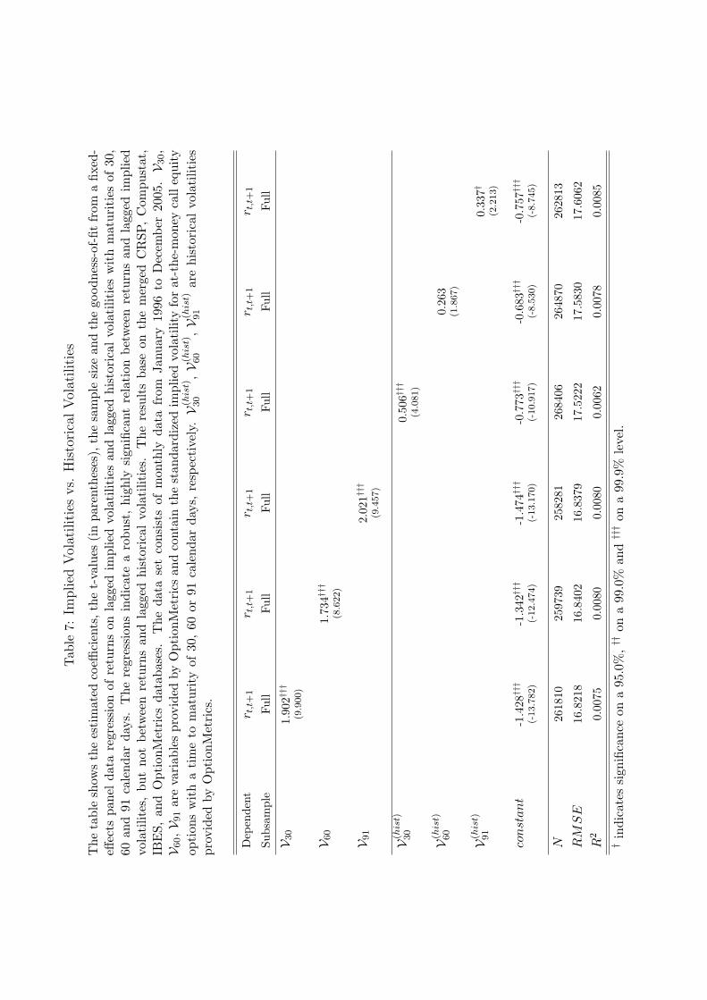
Table 9: Out-of-Sample Performance
The Table shows the the estimated coefficients of a regression of realizedreturns on forecasted returns for a linear, fixed effects model with impliedvolatility as a predictive variable and for the iid model. The out-of-sampleforecast bases on a rolling window with a size of 60 months. RMSE providesthe root-mean-squared-error of the prediction error.
Dependent rt,t+1 rt,t+1
rt,t+1 -0.262†††(-36.048)
riid,t,t+1 -0.293†††(-18.788)
constant -1.169††† -1.169†††(-24.983) (-21.416)
N 126857 126857
RMSE 17.375 16.080
R2 0.0101 0.0028† indicates significance on a 95.0%, †† on a 99.0% and ††† on a 99.9% level.
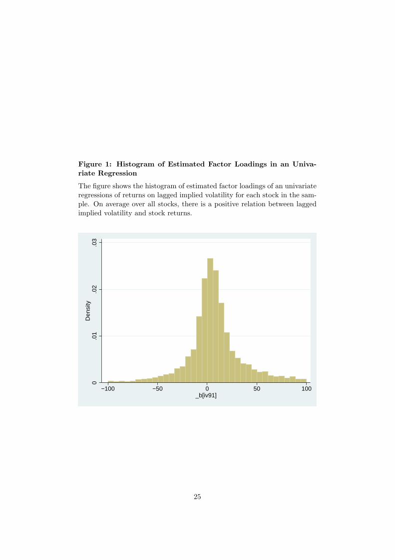
Figure 1: Histogram of Estimated Factor Loadings in an Univa-riate Regression
The figure shows the histogram of estimated factor loadings of an univariateregressions of returns on lagged implied volatility for each stock in the sam-ple. On average over all stocks, there is a positive relation between laggedimplied volatility and stock returns.
0.0
1.0
2.0
3D
ensi
ty
−100 −50 0 50 100_b[iv91]
25
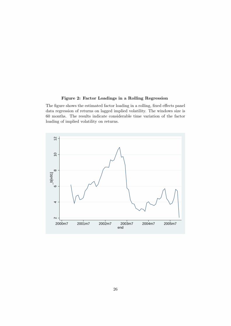
Figure 2: Factor Loadings in a Rolling Regression
The figure shows the estimated factor loading in a rolling, fixed effects paneldata regression of returns on lagged implied volatility. The windows size is60 months. The results indicate considerable time variation of the factorloading of implied volatility on returns.
24
68
1012
_b[iv
91]
2000m7 2001m7 2002m7 2003m7 2004m7 2005m7end
26
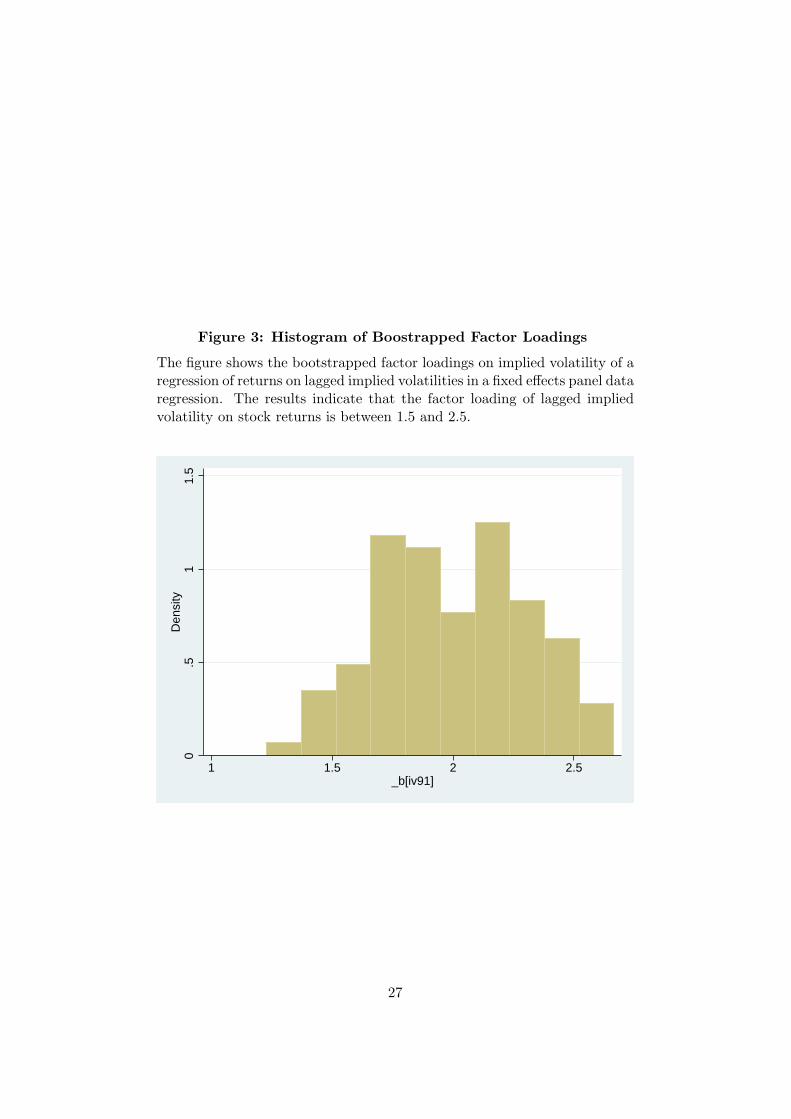
Figure 3: Histogram of Boostrapped Factor Loadings
The figure shows the bootstrapped factor loadings on implied volatility of aregression of returns on lagged implied volatilities in a fixed effects panel dataregression. The results indicate that the factor loading of lagged impliedvolatility on stock returns is between 1.5 and 2.5.
0.5
11.
5D
ensi
ty
1 1.5 2 2.5_b[iv91]
27
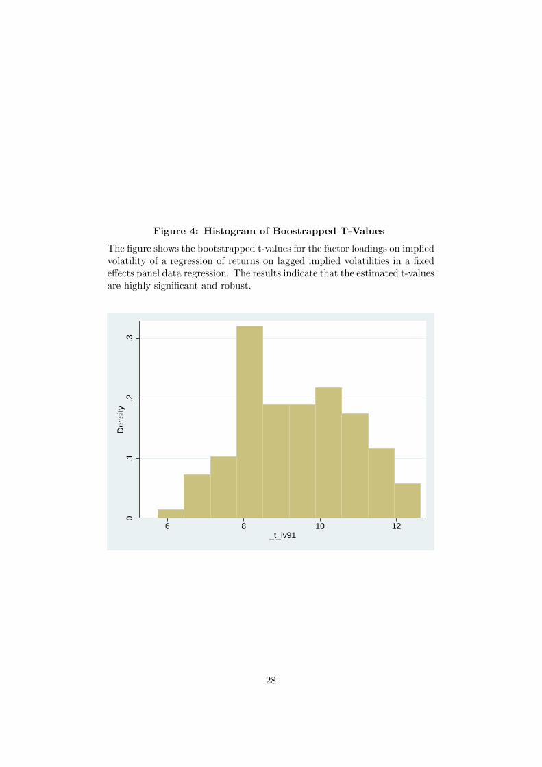
Figure 4: Histogram of Boostrapped T-Values
The figure shows the bootstrapped t-values for the factor loadings on impliedvolatility of a regression of returns on lagged implied volatilities in a fixedeffects panel data regression. The results indicate that the estimated t-valuesare highly significant and robust.
0.1
.2.3
Den
sity
6 8 10 12_t_iv91
28