Volatility as an Asset Class: Holding VIX in a Portfolio

Jared DeLisle

Department of Finance, Insurance, and Real Estate

Washington State University

James S. Doran

Gene Taylor/Bank of America Professor of Finance

Department of Finance

Florida State University

Kevin Krieger

Department of Finance

Tulsa University

March 3, 2010

Keywords: VIX index, S&P 500 Index, Portfolio Returns

JEL Codes: G11, G12

Acknowledgements: The authors acknowledge the helpful comments and suggestions of George Aragon,

Gurdip Bakshi, Michael Brennan, Jim Carson, Don Chance, Martijn Cremers, Sanjiv Das, Dave Humphrey,

Ehud Ronn, Keith Vorkink, David Weinbaum, Xiaoyan Zhang, and participants at the Florida State

University seminar.

Communications Author: James S. Doran Address: Department of Finance

College of Business Florida State University Tallahassee, FL. 32306

Tel.: (850) 644-7868 (Office) FAX: (850) 644-4225 (Office) E-mail: jsdoran@cob.fsu.edu

Abstract

The ability to hedge market downturns without sacrificing upside returns has long been sought by all investors. We consider alternative methods of hedging the S&P 500 with assets that mimic the VIX index in hopes of taking advantage of the asymmetric relationship between volatility and returns. We first demonstrate that if the VIX was investable, and using the fact that volatility mean-reverts, can results in significantly improved portfolio performance over the buy-and-hold index portfolio. However, using VIX futures in a similar fashion does not provide the same results. As such, we deconstruct the VIX Index to find the relevant S&P 500 options that drive the VIX movements. In doing so, we then form a synthetic VIX portfolio using the S&P 500 options and capture returns similar to the VIX index. Our synthetic portfolio is highly liquid and investable, and when combined with a long position in the S&P 500, generates significantly higher returns with lower risk than the buy-and-hold S&P 500 index portfolio.

1

Introduction

Extreme stock market downturns are the most disconcerting periods for investors

since they are risk averse, wish to limit volatility, and seek to avoid negatively skewed

payoffs (Kumar (2009)). Millions of passive investors absorbed massive losses during the

recent stock market retreat which reduced equity indices over 50% from October, 2007 to

March, 2009. The anxiety of such movements even provoked many investors to sell large

portions of equity, mutual fund, and exchange-traded fund (ETF) holdings, thus

guaranteeing large losses.1 The ability to more effectively hedge equity investments with

holdings that would reduce portfolio downside risk over time could combat a considerable

amount of investor unease.

We find that, due to the asymmetric and negative relation between VIX and S&P 500

returns, the VIX index provides a particularly effective hedge against market declines

without proportionally penalizing performance when there are market gains. However,

investors cannot directly invest in the VIX index, and only have exposure to VIX via the

futures and options markets. Our results show that VIX futures are a poor hedging

instrument, while VIX call options provide a good hedge with the added feature of

capturing the positive skewness of the VIX index. We also demonstrate that a new portfolio

strategy involving highly liquid S&P 500 call and put options can be constructed to mimic

the VIX index and thus hedge market losses.

While a number of assets exist with returns that are, on average, negatively

correlated with equities, these instruments may not provide the desired hedge against

market downturns since the return correlations become positive in times of distress. For

1 Mary Pilon, “Many Bought Shares High, Sold Low”, Wall Street Journal, May 18th 2009.

2

example, during the market collapse in 2008, the value of both equities and commodities

fell, though traditionally, commodities are negative beta assets.2 Bond holdings also

declined in value during the 2008 crash, as the need for commercial borrowing declined.

Commercial and residential real estate values dropped greatly, in part due to excessive

leverage, despite the fact that real estate is considered a counter-cyclical investment. Even

many hedge funds, designed to cushion losses in equity markets, saw reversals over the

2007-2009 period. Szado (2009) documents the increased correlation of asset returns over

the crisis period above the levels seen in the 2004-2006 period, implying that as the need

for diversification grew, the ability of many assets to hedge equity holdings shrank at the

most inopportune time. This is why we examine the important question of the ability of the

VIX index to hedge downturns in the equity markets. Holding volatility as an asset class

may make traditional negative or counter-cyclical investments moot for hedging purposes.

Since the introduction of VIX, it has widely been regarded as the economy’s

indicator of risk of the equities market. As noted by Whaley (1993, 2000), the VIX index is

considered “the investors’ fear gauge index.” An important byproduct of introducing VIX

was the newfound opportunity for investors to trade in futures, introduced in March 2004,

and options, introduced in February 2006, thus allowing investors to enter into contracts

and generate payoffs specifically related to volatility. While it is possible to invest in equity

options and futures on the S&P 500 and construct a payoff that would be related to the

volatility of the index, a more direct investment in VIX might require less management of

the position and should provide no tracking error.

2 Numerous commodity indices also retreated by more than 50% of value during the equity market decline of 2007-2009 as inflation ground to a standstill and consumption of raw materials slowed.

3

With more widespread access to market information, VIX has gained increased

exposure in recent years, particularly as it rose to rare levels during the 2008 market

decline. In the wake of increased attention, Whaley (2009) sought to clarify the meaning of

VIX and discuss its characteristics. Whaley (2009) emphasizes that, like the S&P 500 index,

the VIX index is not directly investable. However, while it is quite simple to replicate the

payoff of the S&P 500 by holding the 500 underlying stocks in the appropriate proportions

(or more simply, via investment in low-cost ETFs), it is difficult or impossible to replicate

VIX by holding the underlying S&P 500 options. This is in part because VIX is constructed

using the first two monthly expiration call and put out-of-the money options, with weights

that are squared. Additionally, these weights change daily. Thus, even if a portfolio were

able to hold the correct proportions on a given day, which would require a significant

investment in many option contracts, the next day the proportions would change, and the

rebalancing costs would be prohibitive. As such, the VIX index, viewed as an asset, has been

practically untradeable.

With the availability of futures and options on VIX, it is possible to invest in

volatility, or at least take a position on its future direction. However, it is unclear whether

using the futures or options provides a payoff similar to that of the index, or provides the

hedge against increases in volatilities that investor’s most likely desire. As Szado (2009)

notes, exposure to VIX calls and puts, as well as VIX futures, does not directly mimic

holdings in the spot levels of VIX given that the mean-reverting nature of derivative

instruments are priced into their values.

Because volatility mean-reverts, investing in the VIX index when it is low would

provide protection against volatility increases. Dennis, Mayhew and Stivers (2006) and

4

DeLisle, Doran and Peterson (2010) document the asymmetric relationship between VIX

and the S&P 500 and specifically show that VIX increases and S&P 500 declines are more

strongly correlated than VIX decreases and S&P 500 increases. Whaley (2009) documents

the mean-reverting nature of VIX and also describes its asymmetric nature such that VIX

will rise more (less) dramatically during a stock market decline (rally). Furthermore,

Simon (2003) notes the tendency of traders to overvalue (undervalue) the equity market

when volatility levels are unusually low (high). Consistent with Daigler and Rossi (2006), it

would appear that investing in VIX when it is low not only provides a hedge against

declines in the S&P 500, but will not proportionally penalize investors when the S&P 500

increases.

A number of authors have thus considered the possibility of hedging portfolios with

VIX-mimicking assets. Dash and Moran (2005) initially considered the ability of newly

formed VIX-based products to lower portfolio risk. Emerging possibilities then developed

for such a strategy, including the use of VIX futures, VIX options and VIX-based ETFs.

Brenner, Ou and Zhang (2006) introduce an option on a straddle designed to hedge

volatility risk. This instrument is sensitive to volatility innovations and thus useful as a

hedge. Windcliff, Forsyth and Vetzal (2006) consider the variations in the contract designs

of volatility derivatives and discuss the difficulties of hedging the returns with such

instruments, particularly given delta and delta-gamma hedging techniques. Black (2006)

and Moran and Dash (2007) find that adding VIX futures to a passive portfolio can

significantly reduce portfolio volatility. VIX’s quick movements during risky markets also

improve the skewness and kurtosis of the overall portfolios. Briere, Burgues and Signora

(2010) advocate a sliding approach when hedging in which more (fewer) VIX futures

5

contracts are held when VIX levels are notably lower (higher) due to the mean-reverting

nature of the index.

An important remaining question is the cost-effectiveness of using VIX as a hedging

strategy. If VIX were tradable, we hypothesize that investing in the S&P 500 and VIX, when

VIX is relatively low, would provide investors with a portfolio that will increase in value

when the S&P 500 increases and will be somewhat protected when the S&P 500 falls. Thus,

we wish to explore the profitability of VIX-hedged portfolios to assess the implications of

holding the VIX index alongside the S&P 500. In part, this should reveal whether investing

in the VIX provides an effective hedge to long-equity positions, either through lower costs

or superior returns, than alternative hedges, such as purchasing index puts.

We then explore the benefits of investing in VIX futures and study whether the

futures contracts mimic the payoff to the VIX index. Since these are volatility products that

are tradable, if the payoffs do not replicate the underlying index, it may imply that a

tradable asset on volatility does not provide investors with appropriate protection. Our

results show that this is the case for VIX futures. Next, we examine the benefit of using VIX

call options for portfolio insurance, relative to S&P 500 put options, to assess whether the

payoffs to VIX options provide similar downside protection. We find that VIX options

provide a reasonable hedge, as well as capture the positive skewness of VIX. However, VIX

options are thinly traded in comparison to S&P 500 options, and may present an illiquidity

problem. Finally, we construct a low-cost portfolio that attempts to capture the increases

in VIX by exploring which S&P 500 options drive the changes in VIX. We demonstrate that,

by deconstructing VIX into the individual option components, it is possible to form a

portfolio of liquid S&P 500 options that captures the payoff to the VIX index which eludes

6

the future and option contracts on VIX. This synthetic VIX position improves the hedging

prospects of otherwise passive, long-equity investors.

The rest of the article is as follows: Section I presents the data and its sources,

Section II presents the analyses of the performance of VIX as a hedge against market

declines, Section III investigates which parts of VIX make it a favorable hedge and evaluates

a low-cost portfolio constructed to mimic VIX returns, Section IV concludes the paper.

I. Data

The data for comparison of VIX-based hedging strategies is assembled from

numerous sources. The actual daily VIX levels, utilized for construction of the theoretically

ideal strategy are taken from the CBOE’s historical website.3 The methodology for VIX

construction was amended in September, 2003, though retroactive calculation allows for

collection of data beginning in 1990. Historical S&P 500 returns are taken from CRSP in

order to calculate the returns of positions that theoretically hedge S&P 500 holdings with

the raw VIX level. To adopt actual S&P 500 holdings, we gather price data for the SPY ETF,

which mimics the performance of the S&P 500, also from CRSP.

Futures positions are used as one method for creating a VIX-hedged portfolio. VIX futures

began trading on the CBOE futures exchange in March of 2004. We collect the daily prices

of VIX and S&P 500 futures contracts from the Wall Street Journal archives, beginning with

the arrival of VIX futures.

A second method for assembling a tradable VIX-hedged portfolio is based on the use

of VIX options. These options began trading on the CBOE in February of 2006, and we

3 http://www.cboe.com/micro/VIX/historical.aspx

7

subsequently collect their daily prices from Optionmetrics in order to track the

performance of long-S&P 500 portfolios which are hedged with VIX options.

Additionally, we collect daily data for the S&P 500 index options, SPX, beginning

with the initialization of Optionmetrics in 1996. SPX calls and puts are used to create our

synthetic VIX position, whose returns are tracked through time. While we focus on the

hedging ability that VIX futures and options as well as our synthetic position provide for

holdings of the ETF SPY, we alternatively consider the hedging abilities of S&P 500 put

positions.

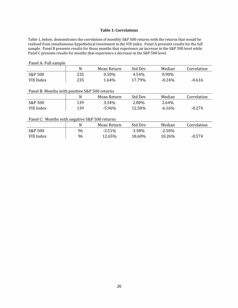
Table 1 presents the summary statistics for S&P 500 and VIX returns. Panel A

shows that S&P 500 returns over the entire sample period average 50 basis points per

month, while VIX returns average 164 basis points per month. However, the standard

deviation of the VIX monthly returns is 17.79%, which is so volatile that the average VIX

returns are statistically indistinguishable from zero. The correlation between S&P 500 and

VIX returns is -0.616, demonstrating a strong negative relation. Panel B limits the sample

to months in which S&P 500 returns are positive. Limiting the sample in this manner

yields average S&P 500 and VIX returns of 3.34 and -5.96 percent per month, respectively.

The correlation between S&P 500 and VIX returns during these months is -0.274. Panel C

shows that the average S&P 500 and VIX returns are -3.51 and 12.65 percent per month,

respectively, when the sample is limited to months where S&P 500 returns are negative.

The return correlation for these months is -0.574. When separating the returns into up and

down periods, mean returns for both the S&P 500 and VIX are significantly different from

zero, highlighting the importance of looking at different market conditions. More

interestingly, the absolute value of the mean S&P 500 returns is similar for up and down

8

market conditions, while the positive mean VIX returns are twice as large during periods of

negative S&P 500 movement as the negative mean VIX returns in periods of positive S&P

500 returns. This result highlights the asymmetric relation between S&P 500 returns and

VIX returns and may be indicative of the potential for using volatility as a hedging

instrument against S&P 500 losses.

II. Effectiveness of VIX as a Hedge Against Market Losses

A. VIX Index as a Hedge

We next examine whether forming portfolios using the VIX index can result in

higher or less volatile returns than passive investing in the S&P 500. While it is not possible

to buy the VIX index, we nonetheless wish to examine whether theoretical holdings in VIX

benefit investors by capturing both the asymmetric relationship between VIX and the S&P

500 and the mean reversion in volatility. We initially examine investing equally in the S&P

500 and the VIX index, and then, given the mean-reversion properties of VIX, we consider

investing in the VIX index only when its level is below certain thresholds. In doing so, the

intent is to capture periods when VIX increases while only investing in the S&P 500 fully

when VIX is falling. The results from the portfolio analyses, based on buying various

combinations of the S&P 500 and VIX indices, are shown in Table 2.

A portfolio made up of strictly the VIX index, shown in Panel A, has a monthly mean return

over the entire sample that is not significantly different from zero, but has statistically

significant CAPM and Carhart (1997) 4-factor model (henceforth just “4-factor”) monthly

alphas of 2.15 and 2.29 percent, respectively. The estimated market betas in the CAPM and

4-factor models are both -2.13 and are highly significant, which is consistent with the

9

negative relationship between the VIX index and the S&P 500. In months with positive S&P

500 returns, the alphas are negative and highly significant while the CAPM market beta and

4-factor market beta are statistically insignificant. Thus, there appears to be only a weak

relation between VIX and market returns when S&P 500 returns are positive. When S&P

500 returns are negative, however, the relationship between VIX returns and the S&P 500

is statistically significant with a CAPM market beta of -1.70 and a 4-factor market beta of -

1.60. If the VIX index could be bought, this asymmetric relationship would imply that the

VIX index can hedge decreases in the S&P 500 without penalizing the portfolio when the

S&P 500 increases. However, even though the relationship is insignificant, the 4-factor

alpha accompanying an S&P 500 increase is -5.07%, and thus it may be desirable to avoid

VIX holdings when the S&P 500 is increasing.

The pertinent question, of course, is when to invest in VIX and when to concentrate

holdings in the S&P 500. While it is practically impossible to forecast when the market is

going up or down, forecasting VIX movements may be easier due to the historically mean-

reverting nature of volatility. Ahoniemi (2008) demonstrates that an ARIMA (1,1,1) model

significantly predicts the directional changes of VIX, thus indicating the mean-reverting

tendency of the index. The historical mean for the VIX index is 22%, which corresponds to

the historical average of volatility for market returns of 19.8%. The VIX index’s mean-

reverting property will tend to move the index back towards the mean when it deviates

greatly from that mean, while the S&P 500 will typically respond in the opposite direction.

Therefore, a naïve strategy of buying the VIX index when it sinks below a certain level may

hedge against future decreases in the S&P 500. To investigate the benefits of investing in

VIX, we consider multiple upper bounds of VIX for such naïve portfolio construction.

10

Panel B of Table 2 presents the performance of portfolios consisting of 50% in the S&P 500

and 50% in the VIX index when VIX is below an indicated level and entirely in the S&P 500

otherwise. The portfolio is rebalanced at the end of each month. A Naïve 20 strategy sets

the maximum VIX-buying level at 20, meaning the portfolio buys VIX if the end-of-the-

month VIX is below 20 and will sell any VIX holdings and place all funds into the S&P 500 if

VIX rises above 20. The mean return for this portfolio is statistically significant, earning

1.54% per month while the CAPM (4-factor) alpha is 1.00% (1.25%). The portfolio’s

market beta for the CAPM (4-factor) case is now a positive 0.48 (0.41), up from the -2.13

reported in panel A and highlighting the effect of VIX on portfolio returns by capturing

positive returns in VIX when the S&P 500 falls. Thus, the Naïve 20 portfolio is positively

related to market returns, but the systematic risk of the portfolio is half that of the market

portfolio and the portfolio returns outperform market returns, even when size, book-to-

market equity ratio, and momentum are accounted for by the 4-factor model.

The allowable VIX-buying level is increased to 25 in the Naïve 25 strategy. The

performance of this portfolio is similar to that of the Naïve 20 portfolio. The main

difference between the two portfolios is that the Naïve 25 portfolio has a market beta that

is not statistically different from zero, indicating that the portfolio has no exposure to

systematic risk. As the VIX-buying level is increased from 25, the portfolios mean returns

and alphas remain similar. However, as the threshold level increases, the market beta of

the portfolio becomes more negative and increasingly significant. For example, the CAPM

market beta for the Naïve 30 portfolio is a statistically significant -0.23 and decreases to -

0.43 for the Naïve 40 portfolio. Increasing the threshold level increases the negative

exposure to systematic risk by holding the VIX index in the portfolio more often.

11

Figure 1 displays the market values of the S&P 500 portfolio and the portfolios

based on the Naïve 20 and Naïve 40 strategies. Each portfolio starts with $100,000 at the

beginning of the year in 1990. Although all naïve portfolios outperform the S&P 500

portfolio, which has a final portfolio value of $0.18 million, and demonstrate the hedging

ability of the VIX index, the buy-and-hold returns of the strategies differ dramatically. The

Naïve 20 portfolio has an ending market value of $2.12 million, while the Naïve 40 portfolio

has an ending value of $0.92 million. Thus, while the mean returns and alphas appear

similar, the buy-and-hold (BHR) returns tell a very different story. Table 3 shows the BHRs

for each portfolio and the corresponding risk.

B. VIX Futures as a Hedge

The portfolios examined above rely on the ability to buy and sell the VIX index

which, currently, is not a possibility. However, since April 2004, it has been possible for a

portfolio to buy or sell cash-settled VIX futures. Since entering into VIX futures may be a

close substitute to theoretical investment in the VIX index, we wish to investigate whether

investing in the VIX futures actually replicates the payoff of the index. Panel A of Table 4

shows the mean returns and alphas from a portfolio that invests in one-month VIX futures

contracts, entering into new contracts when the prior month contracts expire.

A portfolio that invests in VIX futures, starting with the availability of futures data in

April 2004, through the end of August 2009, returns a statistically insignificant -3.12% a

month. By comparison, the monthly return of the VIX index over the same period was 1.8%

12

per month. When separated into periods of positive and negative S&P 500 returns,4 the

returns to VIX futures contracts are more negative when the S&P 500 is increasing, while

the opposite is true of the VIX index itself.5 The difference between mean returns of the VIX

futures and the index were -4.73% when S&P 500 futures fell and -6.84% when S&P 500

futures rose. Thus, the holders of futures contracts overpaid relative to the index

regardless of the direction of the S&P 500 futures returns. This contrast between the VIX

futures and the index suggests the futures contracts did not offer the same downside

protection investors would expect given the asymmetric relationship between volatility

and returns.

Panel B of Table 4 demonstrates the poor performance of the naïve strategies using

futures contracts on the S&P 500 and VIX indices.6 The mean returns and alphas of all the

portfolios are negative and statistically significant for the Naïve 20 and Naïve 25 futures

portfolios. Figure 2 displays the market value of the Naïve 20 and Naïve 40 futures

portfolios over time, along with a portfolio in S&P 500 futures, and demonstrates the poor

performance of incorporating VIX futures in a portfolio. By comparison, over the same

holding period, the Naïve 20 portfolio using the actual VIX index would have doubled in

value. The poor performance of the futures may be due to their term structure where

sellers of the futures incorporate a premium for the upside risk in the index futures, since

on average, VIX futures have an upward sloping term-structure.

4 In order to match the term structure of the VIX index futures, the portfolio should contain S&P 500 index futures of similar maturity rather than the S&P 500 index itself. 5 For the same periods, when the S&P 500 was falling (rising), the VIX index increased (decreased) on average by 17.0% ( -8.2%). 6 Results are similar using the S&P 500 index returns.

13

C. VIX Options as a Hedge

Since VIX calls became available to trade in March 2006, we compare the hedging

ability of these options to using S&P 500 puts to hedge downside risk exposure to market

movements. Specifically, we are interested in two aspects of VIX calls as an alternative type

of portfolio insurance; first, the cost of the insurance, and second, the options’ ability to

capture the asymmetric relation between volatility and returns.

The construction of the hedged portfolio assumes a long position in the S&P 500

index by purchasing shares of the index-tracking ETF, SPY. The portfolio holds the initial

position, or shares in the SPY, constant throughout the evaluation period. In order to hedge

this position, the portfolio simultaneously purchases the requisite number of near-term,

ATM, S&P 500 puts or VIX-Index calls, and holds the contracts to expiration. On the

following Monday, the portfolio then enters into new near-term contracts, hedging the

same number of underlying shares. This keeps the hedge position identical each period as

only the cost of the hedge, which is a function of market volatility, and the payoff to the

options, will vary. This allows us to keep track of the cost, payoff, and effectiveness of each

strategy by observing the change in portfolio value. The hedge portfolio will alternatively

utilize 5% OTM contracts for both S&P 500 puts and VIX-Index calls to account for

potential moneyness effects.

Since we wish to compare the cost and performance of the two hedging strategies,

we assume the same dollar value of options is purchased each month for both S&P 500 puts

and VIX Index calls. As a result, many more VIX options may be purchased. For example, if

the S&P 500 index level was 1067, and the portfolio held 100 shares in the index, we could

buy one put with a strike price of 1065 for $30. If the VIX index was at 25, the alterative

14

portfolio could buy 10 calls at a price of $3 each.7 Each position would cost $3000. If the

index fell to 1000, the put would result in a payoff of $6500 minus the original $3000 cost.

The payoff to the VIX calls would be equivalent to the S&P 500 put if the index increased to

31.5. Ultimately, we are interested in discovering how the VIX index tends to react in these

situations, and whether it is a more or less effective hedge when the S&P 500 is falling.

Alternatively, the portfolio could hold fewer VIX-call options, though it is easier to assess

the performance of the hedge by allowing only the payoffs from the options to deviate.

Figure 3 demonstrates the performance of the VIX-call and S&P 500-put hedge

strategies from March 2006 through October 2009. From the beginning of the evaluation

period through the summer of 2008, there are instances when the payoff to one strategy

may be slightly higher than the other, but the value of the portfolios remain similar. This is

unsurprising given the high negative correlation between the VIX index and the S&P 500. It

is also not surprising that the hedge portfolios underperform while the S&P 500 was

generally growing steadily since the cost of portfolio insurance is expensive (Bates (2000)).

However, starting in September 2008, when the markets began falling and volatility rose to

historic levels, the payoff of the VIX-call strategy drastically outperforms the S&P-put

hedge. While this is partly the result of holding more call options, it is mainly due to the

ability of VIX calls to capture the positive skewness in volatility that the S&P 500 puts

cannot capture. The fall in the S&P 500 from July through November 2008 was over 36%,

but the corresponding increase in the VIX index was 300%. This resulted in an increase in

value of about 50% in the portfolio that used VIX calls as a hedge, while the portfolio that

used S&P 500 puts still declined 20%. This suggests that to hedge significant market

7 Actual prices on 2/11/2010

15

declines, calls on volatility are better instruments to use than puts on the S&P 500 index

because positive skewness in volatility is unbounded.

Hedging simple, passive positions like long-S&P 500 with VIX calls, rather than S&P

500 puts, appears to be an attractive alternative even though both options are expensive. It

is the ability of VIX calls to capture positive skewness that suggests they are a superior

alternative. What remains unclear is whether the difference in the payoffs in the two

hedging strategies is due to underpricing of VIX calls or overpricing of S&P 500 puts. There

is recent evidence that suggests negative skewness is priced in equity returns (Boyer,

Mitton and Vorkink (2009)) and index option prices (Doran and Krieger (2010)). Our

portfolio result suggests that the options on volatility have not incorporated corresponding

positive skewness or the increase in skewness in VIX relative to the decrease in skewness

in the index. As such, it appears that VIX calls are cheap only because of the differences in

underlying return distributions of volatility and equity instruments, not necessarily

because they are mispriced.

III. Replicating the VIX index

A. Decomposing VIX

While numerous studies have analyzed the impact of the VIX Index, or changes in

VIX, on the returns of equity portfolios, few have considered what drives the actual changes

in VIX itself. Whaley (2009) examined the effect of changes in the S&P 500 index on VIX

changes and found an asymmetric response to those changes. This is not surprising and

consistent with the results of DeLisle, Doran and Peterson (2010). However, to this point,

there has been no examination based on the actual options that cause VIX to change. Since

16

the VIX Index is constructed using only near-term and 2nd near-term month closest to ATM

and all out-of-the money puts and calls on the S&P 500, it is worth testing which options

drive the movement of VIX. Since there is an asymmetric response between changes in the

S&P 500 and VIX, it is highly likely that puts versus calls, ATM versus OTM, or near-term

versus 2nd near-term monthly expiration discrepancies are responsible for the changes.

Before deriving an empirical specification to test the relationship between S&P 500

options and VIX changes, we briefly summarize the methodology used to calculate the VIX

Index. The specification for VIX is given by:8

��� � �� ∑ ��

���� ���� � �

� ����� � 1��

� (1)

��� � 100�� ���� !"#$"%�"#$"#&

' ( ���� !"%�$"#&"#$"#&

') "%*+"%� (2)

where � is the strike price of options that are currently closest to ATM or OTM, ∆� is the

difference in strike prices, ���is the midpoint price of the option at strike �, �is the

expiration of the near-term option, �is the expiration of the 2nd near-term option, N is the

minutes to expiration and - represents the ATM forward price of the index. Using all

options available that are closest to ATM and OTM, equation (1) constructs a ��� for both

the near-term and 2nd near-term options, while equation (2) weights the ��� to create a 30-

day measure of implied volatility.

While both equations are straightforward to calculate and recreate the current level

of VIX, the non-linear nature makes replicating the payoff to the VIX index difficult to

8 A white paper available from CBOE at http://www.cboe.com/micro/vix/vixwhite.pdf shows the construction of the VIX index.

17

accomplish. The weight on each option is a function of a root-weighted time variable, which

changes daily, making rebalancing costs prohibitive while creating indivisible option units.

However, it is possible to unwind the formula into smaller components, allowing for a test

of the effect of each option, or the changes in the prices and moneyness of each option, on

the changes in VIX.

Taking the natural log of equation (2) removes the nonlinear term such that

equation (2) become linear, and allows for a simple regression to assess the impact of the

individual options on the change in VIX. Since we are interested in changes, testing the

difference between ln����1� � ln ����1$��, is equivalent to testing ln 2 345634567&8, or the

percentage change in VIX each day. The key explanatory variables to include are whether

the option was a call or a put, the time to expiration of the option, the price change, the

strike price or moneyness change, and an interaction term between these variables. It is

necessary to incorporate an interaction term, since the first term in equation (1) is

multiplicative in these variables.

We run the following specifications, controlling for time variation,

ln 2 345634567&8 � 91 ( Δ;<,>,?,@+ Δ�A<,>,?,@ ( BC<,>,?,@ ( �<,>,?,@

(Δ;<,>,?,@ D EB1 ( Δ�A<,>,?,@ D EB1 ( F1 (3)

ln 2 345634567&8 � 91 ( Δ;<,>,?,@+ Δ�A<,>,?,@ ( BC<,>,?,@ ( �<,>,?,@ ( F1 (4)

Where Δ;<,>,τ,@is the change in price of G(call/put) option with a strike of � and maturity H

at time t. Δ�A represents the change is moneyness of the option, where put moneyness is

equal to S/K and call moneyeness is equal to K/S. Thus, more positive changes bring both

definitions of moneyness closer to ATM. BC is the time to maturity of the option, and � is

18

the interaction of all three variables. EB is a dummy variable equal to one if the option is a

call and zero if the option is a put. Equation (3) interacts the dummy variables with change

in price and moneyness variables to capture differences between call and put options.

Equation (4) examines the effect of price and moneyness changes of calls and puts

separately on VIX changes. Each specification clusters on the date to avoid overstating the

t-stats. The results are shown in Table 5.

We conduct seven estimations with the first three using equation (3) and the final

four using equation (4). The first utilizes the full sample while the second (third) considers

the positive (negative) VIX changes only. The fourth and fifth estimations use only puts and

segment the sample based on whether VIX is above and below the historical mean of 22.

The last two estimations use only calls, again segmenting the sample based on VIX levels

above and below 22.

The results of the first estimation reveal that increases in price are positively related

to VIX changes. Specifically, if the option becomes one dollar more expensive, then VIX will

increase by 0.25% on average. However, if the option is a call, for each dollar increase the

change in VIX is only 0.11% as the coefficient of the call dummy is -0.14. This suggests a

greater impact from put price changes than call price changes. Options that are closer to

ATM have a greater effect on VIX values, as a 0.01 increase in moneyness results in an

increase of 3.32% in VIX. Again, this is only for puts, because as call options approach ATM

status, the effect on VIX is a fall of -4.01%. This is consistent with negative correlation

between VIX and the S&P 500 since puts (calls) become more expensive as the S&P 500

falls (increases). There is no significant relationship with the expiration of the option,

19

although the negative coefficient on DM is consistent with a negative option theta. The

interaction term is positive, as expected, but the effect on the change in VIX is small.9

The results of the second and third estimation are similar in direction for all the

coefficients, but the interpretation of the coefficients reveals interesting results. The

coefficient on Δ; is 0.141 larger and statistically different than the Δ; coefficient when VIX

is increasing versus decreasing, suggesting an asymmetric response to put price changes

on VIX changes. Also the discrepancy between put and call price changes on VIX changes is

larger when VIX is increasing. When VIX decreases, Δ; D EB is insignificant, again

highlighting the importance of put price changes for VIX increases, which are highly

negatively correlated with negative S&P returns. The results of the final four estimations

further emphasize these findings. Put price changes have a greater effect on VIX changes at

all levels of VIX, relative to calls, but the effect is especially strong for VIX levels less than

the mean.

These results suggest that ATM put options are most responsible for driving

changes in VIX, and this appears particularly true when VIX is below its historical mean.

Given these findings, and because we are interested in investing in a portfolio that has

returns corresponding to the VIX index, in order to hedge against downturns in the market,

holding a portfolio that is long in ATM S&P 500 puts appears to be a natural fit. However, it

has been well documented that puts are expensive.10 Thus, it is necessary to not only go

long puts, but sell either OTM puts or corresponding calls to offset the cost. Given the

9 A one dollar change times a 0.01 change in moneyness for a one-month option, multiplied by the 48.47 coefficient on I, results in a 0.02% change in VIX. 10 For example, Jackwerth (2000), Aït-Sahalia, Wang and Yared (2001), Coval and Shumway (2001), Bakshi and Kapadia (2003), Bondarenko (2003), Bollen and Whaley (2004), and Liu, Pan and Wang (2005) generally find that the historical costs of puts, particularly OTM and ATM puts, are too expensive to be justified.

20

results in Table 5, we opt to form a zero-cost portfolio that will buy ATM puts and OTM

calls and sell OTM puts and ATM calls, where the ratio of calls to puts will be determined by

the level of VIX and the coefficients on the price.

Since one of the hurdles in replicating VIX is the difficulty in daily rebalancing costs

of the options, our replicating portfolio will enter into the zero-cost investment at the

beginning of the month, using both the near-term and 2nd near-term options only. The

investment in the options will only occur if the level of the VIX index is below 35 since our

earlier results have shown the negative correlation and asymmetric response between the

VIX index and the S&P 500. The portfolio will hold the equivalent number of options

corresponding to 100 shares in the index, while accounting for the margin required by

selling options. As such, less total investment can be made in the S&P 500 since cash needs

to be set aside to maintain the margin account. In addition, there may be instances when

additional cash is needed to cover potential margin calls. Should this occur, shares from the

underlying will be sold to make up cash shortfalls.

B. Performance of VIX Replication

Figure 4 shows the return to a portfolio that initially invests $100,000 in either the

S&P 500 or the S&P 500 and the synthetic VIX portfolio, starting January 1996 and ending

October 2009. The return to the portfolio that incorporates the replicating VIX strategy

outperforms the buy-and-hold S&P 500 portfolio significantly. The annualized return to

hedged portfolio is 12.4% with an annual volatility is 18.6%. The return is 6.5% higher

than the S&P 500 buy-and-hold portfolio with almost identical risk. The alpha from a

market model regression is 6.9% and is highly significant, but becomes insignificant if VIX

21

is included in the specification. This suggests that our replicating portfolio does a good job

of capturing the hedging benefits of holding the VIX index.

Using different levels of VIX as the threshold level has a minimal effect on the overall return

to the replicating portfolio unless the threshold level of VIX is above 45 or below 20. If a

threshold level of 20 is used, then the hedge does not cover large declines in the S&P 500.

When an investment is made with VIX above 45, the return to the hedge portfolio is

negligible because these periods tend to be uncorrelated to the increases in the S&P 500.

There is a specific downside to the synthetic VIX portfolio approach. It cannot

capture the positive skewness in the VIX index. Hedging skewness in VIX, which

corresponds to large increases in the index or sharp declines in the S&P 500, is very costly

and thus not worth implementing. For example, from September through November of

2008, when the S&P 500 fell over 400 points and VIX increased from a level of 20 to the

high 80’s, the replicating strategy would have lost significantly because the OTM puts

would have paid off significantly more than the ATM options. This also would have

occurred in March and September/October of 2001 and July 2002, when VIX spiked and the

S&P fell sharply. In total, the hedge portfolio would lose 7 out of 168 months in our sample;

however, while the frequency is rare, the losses would have been large.

Such risks, if hedged, would cost more than the total gains, and are risks we feel are

acceptable. Since the replicating portfolio captures the asymmetric relationship between

volatility and returns, it captures most of the downside risk investors wish to hedge. The

fact that the portfolio does not capture the skewness is unfortunate, but is a risk that as of

now appears unavoidable. A potential alternative to hedging skewness is reverting to VIX

calls. Figure 3 highlights the ability of the VIX calls to hedge the market decline in late 2008

22

as a result of the positive skewness in the VIX index. Thus a portfolio that combined our

replicating strategy with some VIX calls may be the ideal hedging combination.

IV. Conclusion

Our results indicate the effectiveness and importance of holding volatility as an

asset class in avoiding market shortfalls by hedging downside risk. Since the current

asymmetric relationship between the VIX index and the S&P 500 generates the strongest

correlations when the market is falling, holding the VIX long is a natural candidate for

hedging market risk while still providing upside return potential. Our results show that if

VIX were investable, a portfolio comprised of VIX and the S&P 500 would provide returns

and risk that far outpace the traditional buy-and-hold portfolio.

Of course, those initial results are hypothetical, and moreso, un-replicable via VIX

futures or options because they do not capture the same properties that characterize the

index, particularly, mean reversion. The portfolio of holding VIX futures in combination

with either the S&P 500 or futures on the S&P 500 significantly underperforms. This result

is disappointing since VIX futures do not offer the payoff to volatility that investors would

expect. It is not clear if this is due to low liquidity or mispricing of futures contracts, since it

is not possible to arbitrage mispricing by holding the underlying.

By dissecting the VIX into the individual options that are responsible for the index

change, we demonstrate that S&P 500 puts closest to ATM are most responsible for the VIX

movements, especially when volatility increases. With this understanding, we are able to

form a portfolio which holds the S&P 500 option contracts that best capture increases in

VIX while selling other contracts to form a zero-cost investment portfolio. Our synthetic

23

VIX portfolio is quite liquid, unlike VIX calls to date, and performs extremely well, capturing

the increases in VIX without proportionally penalizing the portfolio when the market

increases. While this portfolio does require the use of margin, it neutralizes the downside

market risk investors wish to remove while allowing for the upside gain. The aspect it

cannot capture is positive skewness in volatility. However, through holding VIX calls, we

demonstrate new hedges for traditional passive long strategies which are a much more

effective (or cost-effective) portfolio insurance than buying S&P 500 puts.

24

References

Ahoniemi, Katja, 2008, Modeling and forecasting the vix index, Working paper.

Aït-Sahalia, Yacine, Yubo Wang, and Francis Yared, 2001, Do option markets correctly price the

probabilities of movement of the underlying asset?, Journal of Econometrics 102, 67-110.

Bakshi, Gurdip, and Nikunj Kapadia, 2003, Delta-hedged gains and the negative market volatility risk

premium, Review of Financial Studies 16, 527-566.

Bates, David S., 2000, Post-'87 crash fears in the s&p 500 futures option market, Journal of Econometrics

94, 181-238.

Black, Keith, 2006, Improving hedge fund risk exposures by hedging equity market volatility, or how the

vix ate my kurtosis, Journal of Trading Spring, 6-15.

Bollen, Nicolas P. B., and Robert E. Whaley, 2004, Does net buying pressure affect the shape of implied

volatility functions?, The Journal of Finance 59, 711-753.

Bondarenko, Oleg, 2003, Why are put options so expensive, Working paper.

Boyer, Brian, Todd Mitton, and Keith Vorkink, 2009, Expected idiosyncratic skewness, Review of

Financial Studies 23, 169-202.

Brenner, Menachem, Ernest Y. Ou, and Jin E. Zhang, 2006, Hedging volatility risk, Journal of Banking &

Finance 30, 811-821.

Briere, Marie, Alexandre Burgues, and Ombretta Signora, 2010, Volatility exposure for strategic asset

allocation, Journal of Portfolio Management forthcoming.

Carhart, Mark M., 1997, On persistence in mutual fund performance, The Journal of Finance 52, 57-82.

Coval, Joshua D., and Tyler Shumway, 2001, Expected option returns, The Journal of Finance 56, 983-1009.

Daigler, R.T., and L. Rossi, 2006, A portfolio of stocks and volatility, Journal of Investing Summer, 99-106.

Dash, Srikant, and Matthew T. Moran, 2005, Vix as a companion for hedge fund portfolios, Journal of

Alternative Investments Winter, 75-80.

DeLisle, R. Jared, James S. Doran, and David R. Peterson, 2010, Asymmetric pricing of implied

systematic volatility in the cross section of expected returns, Journal of Futures Markets forthcoming.

Dennis, Patrick, Stewart Mayhew, and Chris Stivers, 2006, Stock returns, implied volatility innovations, and the asymmetric volatility phenomenon, Journal of Financial and Quantitative Analysis 41,

381-406.

Doran, James S., and Kevin Krieger, 2010, Implications for asset returns in the implied volatility skew,

Financial Analysts Journal 66, 65-76.

25

Fama, Eugene F., and Kenneth R. French, 1993, Common risk factors in the returns on stocks and bonds,

Journal of Financial Economics 33, 3-56.

Jackwerth, JC, 2000, Recovering risk aversion from option prices and realized returns, Review of

Financial Studies 13, 433-451.

Kumar, Alok, 2009, Who gambles in the stock market?, The Journal of Finance 64, 1889-1933.

Liu, Jun, Jun Pan, and Tan Wang, 2005, An equilibrium model of rare-event premia and its implication for option smirks, Review of Financial Studies 18, 131-164.

Moran, Matthew T., and Srikant Dash, 2007, Vix futures and options, pricing and using volatility products to manage downside risk and improve efficiency in equity portfolios, Journal of Trading

2, 96-105.

Simon, David, 2003, The nasdaq volatility index during and after the bubble, Journal of Derivatives 11, 9-24.

Szado, Edward, 2009, Vix futures and options: A case study of portfolio diversification during the 2008 financial crisis, Journal of Alternative Investments 12, 66-85.

Whaley, Robert, 1993, Derivatives on market volatility: Hedging tools long overdue, Journal of

Derivatives 1, 71-84.

Whaley, Robert, 2000, The investor fear gauge, Journal of Portfolio Management 26, 12-17.

Whaley, Robert, 2009, Understanding the vix, Journal of Portfolio Management 3, 98-105.

Windcliff, H., P. A. Forsyth, and K. R. Vetzal, 2006, Pricing methods and hedging strategies for volatility derivatives, Journal of Banking & Finance 30, 409-431.

26

Table 1: Correlations

Table 1, below, demonstrates the correlation of monthly S&P 500 returns with the returns that would be realized from simultaneous hypothetical investment in the VIX index. Panel A presents results for the full sample. Panel B presents results for those months that experience an increase in the S&P 500 level while Panel C presents results for months that experience a decrease in the S&P 500 level.

Panel A: Full sample

N Mean Return Std Dev Median Correlation

S&P 500 235 0.50% 4.54% 0.90% VIX Index 235 1.64% 17.79% -0.24% -0.616

Panel B: Months with positive S&P 500 returns

N Mean Return Std Dev Median Correlation

S&P 500 139 3.34% 2.80% 2.64% VIX Index 139 -5.96% 12.50% -6.16% -0.274

Panel C: Months with negative S&P 500 returns

N Mean Return Std Dev Median Correlation

S&P 500 96 -3.51% 3.38% -2.50% VIX Index 96 12.65% 18.60% 10.26% -0.574

27

Table 2: VIX Index Portfolio Returns

Table 2, below, provides return and abnormal return measures for hypothetical holdings of the VIX index. Panel A gives monthly results for the VIX index when all observation months are included, and then, separately, for months when positive (negative) S&P 500 returns are realized. Panel B gives monthly results for the naïve strategies which invest equally in the hypothetical VIX and the S&P 500 when VIX levels are below the numerical level presented and entirely in the S&P 500 otherwise. Mean monthly returns are presented, as are the CAPM alpha and beta which result from the regression of monthly portfolio returns on the value-weighted monthly market return, and the Carhart (1997) 4-factor alpha and market beta which result from the regression of monthly returns on the three Fama and French (1993) factors (MKT, SMB, and HML) and Carhart’s (1997) momentum factor (UMD), which are obtained from Ken French’s website. Test statistics are given in parentheses. *, ** and *** denote statistical significance at the 10%, 5% and 1% levels, respectively.

Panel A: VIX index portfolio results Mean CAPM MKT

Beta CAPM Alpha

4-Factor MKT Beta

4-Factor Alpha

Full sample 1.64 -2.13*** 2.15** -2.13*** 2.29**

(1.41) (-9.65) (2.28) (-8.55) (2.25)

Months S&P 500 returns>0 -5.96*** -0.77* -3.95** -0.36 -5.07***

(-5.63) (-1.82) (-2.36) (-0.75) (-2.83)

Months S&P 500 returns<0 12.65*** -1.70*** 6.44** -1.60*** 7.78***

(6.66) (-3.64) (2.67) (-3.13) (3.09)

Panel B: Portfolio Strategy Mean CAPM MKT

Beta CAPM Alpha

4-Factor MKT Beta

4-Factor Alpha

Naïve 20 1.54*** 0.48*** 1.00** 0.41*** 1.25***

(3.39) (5.00) (2.31) (3.80) (2.82)

Naïve 25 1.57*** 0.04 1.21** -0.40 1.44***

(3.13) (0.37) (2.38) (-0.29) (2.81)

Naïve 30 1.46 -0.23** 1.22** -0.23* 1.35**

(2.85) (-1.97) (2.38) (-1.77) (2.58)

Naïve 35 1.13 -0.31** 0.92* -0.28** 0.96*

(2.18) (-2.72) (1.79) (2.20) (1.82)

Naïve 40 1.29 -0.43*** 1.13** -0.44*** 1.25**

(2.51) (-3.85) (2.24) (-3.53) (2.43)

28

Table 3: VIX Index Buy and Hold Returns

Table 3, below, gives the overall and monthly mean returns for investment strategies which include holdings in either the S&P 500, the hypothetical VIX asset, or both in the naïve strategy cases. The naïve strategies invest equally in the hypothetical VIX and the S&P 500 when VIX levels are below the numerical level presented and entirely in the S&P 500 otherwise.

Overall BHR (%)

Mean Monthly BHR (%)

Std Dev of Monthly BHR(%)

S&P 500 178.75 0.44 4.69

VIX 48.26 0.17 18.56

Naïve 20 2022.19 1.31 7.02

Naïve 25 1933.85 1.29 7.74

Naïve 30 1428.65 1.17 7.91

Naïve 35 595.96 0.83 8.00

Naïve 40 922.84 0.99 7.89

29

Table 4: VIX Futures Portfolio Returns

Table 4, below, provides monthly return and abnormal return measures for holdings of VIX futures. Panel A gives monthly results for VIX futures when all observation months are included, and then, separately, for months when positive (negative) S&P 500 returns are realized. Panel B gives monthly results for the naïve strategies which invest equally in VIX futures and the S&P 500 when VIX levels are below the numerical level presented and entirely in the S&P 500 otherwise. Mean monthly returns are presented, as are the CAPM alpha and beta which result from the regression of monthly portfolio returns on the value-weighted monthly market return, and the Carhart (1997) 4-factor alpha and market beta which result from the regression of monthly returns on the three Fama and French (1993) factors (MKT, SMB, and HML) and Carhart’s (1997) momentum factor (UMD), which are all obtained from Ken French’s website. The mean return from the VIX index portfolio over the same time period are also presented in Panel A for comparison purposes. Test statistics are given in parentheses. *, ** and *** denote statistical significance at the 10%, 5% and 1% levels, respectively.

Panel A: VIX Futures portfolio results VIX Futures

Mean Return VIX Index

Mean Return CAPM MKT

Beta CAPM Alpha

4-Factor MKT Beta

4-Factor Alpha

Full sample -3.12 2.83 -3.80*** -3.65** -4.21*** -3.80**

(N=59) (-0.95) (0.94) (-11.08) (-1.97) (-10.19) (-2.12)

Months S&P 500 Futures returns>0 -14.07*** -7.23*** -0.96* -11.53*** -1.13 -10.83***

(N=34) (-8.44) (-3.14) (-1.70) (-5.01) (-1.33) (-3.77)

Months S&P 500 Futures returns<0 11.78* 16.51*** -5.05*** -9.43** -5.30*** -10.29**

(N=25) (1.87) (3.09) (-8.92) (-2.45) (-7.61) (-2.69)

Panel B: Portfolio strategy results VIX Futures

Mean Return CAPM MKT

Beta CAPM Alpha

4-Factor MKT Beta

4-Factor Alpha

Naïve Futures 20 -2.30** 0.40** -2.51*** 0.29 -2.44***

(-2.72) (2.64) (-3.12) (1.58) (-3.14)

Naïve Futures 25 -1.97** 0.06 -2.20** -0.17 -2.21**

(-2.18) (0.36) (-2.42) (-0.79) (-2.46)

Naïve Futures 30 -1.02 -1.08*** -1.31 -1.57*** -1.42

(-0.79) (-5.30) (-1.22) (-7.19) (-1.53)

Naïve Futures 35 -1.27 -1.09*** -1.56 -1.60*** -1.67*

(-0.98) (-5.33) (-1.45) (-7.37) (-1.81)

Naïve Futures 40 -1.57 -1.17*** -1.87* -1.59*** -2.02**

(-1.22) (-5.98) (-1.81) (-7.29) (-2.18)

30

Table 5: VIX Factor Regression

Table 5, below, shows the results from the following regressions:

ln 2 345634567&

8 � 91 ( Δ;<,>,?,@+ Δ�A<,>,?,@ ( BC<,>,?,@ ( �<,>,?,@ ( Δ;<,>,?,@ D EB1 ( Δ�A<,>,?,@ D EB1 ( F1 and

ln 2 345634567&

8 � 91 ( Δ;<,>,?,@+ Δ�A<,>,?,@ ( BC<,>,?,@ ( �<,>,?,@ ( F1

Where Δ;<,>,τ,@is the change in price of G(call/put) option with a strike of � and maturity H at time t.

Δ�A represents the change is moneyness of the option, where put moneyness is equal to S/K and call moneyeness is equal to K/S. Thus, more positive changes bring both definitions of moneyness closer to ATM. BC is the time to maturity of the option, and � is the interaction of all three variables. EB is a dummy variable equal to one if the option is a call and zero if the option is a put. The first regression interacts the dummy variables with change in price and moneyness variables to capture differences between call and put options. The second regression examines the effect of price and moneyness changes of calls and puts separately on VIX changes. Each specification clusters the standard errors by date to avoid overstating the t-statistics. Test statistics are given in parentheses. *, ** and *** denote statistical significance at the 10%, 5% and 1% levels, respectively.

∆VIX ∆VIX >0 ∆VIX <0

Puts Only VIX>22

∆VIX

Puts Only VIX<22

∆VIX

Calls Only VIX>22

∆VIX

Calls Only VIX<22

∆VIX

ΔP 0.248 0.339 0.198 0.203 0.818 0.112 0.346

(7.36)** (4.91)** (7.98)** (6.67)** (9.18)** (3.81)** (4.70)**

ΔKS 331.813 210.608 172.541 301.053 448.465 -364.368 -636.329

(32.68)** (13.11)** (16.07)** (27.59)** (21.61)** (33.74)** (21.62)**

DM -1.031 -1.292 0.55 -0.922 -4.73 -0.197 -3.983

(1.35) (1.25) (0.76) (0.91) (3.12)** (0.17) (2.62)**

ΔP*CD -0.14 -0.262 -0.043

(3.88)** (2.80)** (1.06)

ΔKS*CD -732.004 -510.739 -407.071

(38.11)** (17.27)** (19.58)**

I 48.473 15.45 19.685 38.079 456.779 44.168 413.826

(4.76)** -0.69 (4.80)** (4.61)** (4.42)** (2.64)** (3.38)**

Constant 0.26 2.958 -2.622 0.427 0.533 0.306 0.381

(2.85)** (24.20)** (31.39)** (3.63)** (3.94)** (2.33)* (2.37)*

OBS 33681 15813 17718 9437 8177 9358 6682

R-squared 0.57 0.39 0.35 0.61 0.55 0.65 0.57

31

Figure 1: VIX Index Portfolio Returns

Figure 1, below, tracks the performance of investment strategies incorporate the holding of the hypothetical VIX asset. Naïve 20 (40) holds hedging positions in the hypothetical VIX asset when a calendar month begins with a VIX level less than 20 (40) and holds only the S&P 500 otherwise. Hedging consists of utilizing half of available funds to go long in the hypothetical VIX asset. Buy-and-hold positions with monthly formation are tracked beginning with the availability of historical VIX data.

$0

$500,000

$1,000,000

$1,500,000

$2,000,000

$2,500,000

$3,000,000

S&P_Port Naïve_20 Naïve_40

32

Figure 2: VIX Futures Portfolio Returns

Figure 2, below, demonstrates the returns to an investment strategy which commences investment in S&P 500 futures in March of 2004 when VIX futures were introduced. An approach which invests in S&P 500 futures and reinvests after each futures contracts’ expiration is shown. Additionally, a Naïve 20 (40) strategy is considered which invests half of the available funds in VIX futures when the VIX level is below 20 (40) at the previous futures expiration date.

$0

$20,000

$40,000

$60,000

$80,000

$100,000

$120,000

$140,000

$160,000

S&P 500 Futures Futures_20 Futures_40

33

Figure 3: Hedging Using VIX Calls

Figure 3, below, demonstrates the returns to an investment strategy which commences investment in the S&P 500-tracking ETF, SPY beginning in May of 2006 with the introduction of VIX options data. Approaches which invest in SPY at the beginning of the study period and concurrently invest in options to form delta-neutral portfolios are analyzed. The use of VIX calls and, S&P 500 puts as hedging instruments are alternatively considered.

$0

$20,000

$40,000

$60,000

$80,000

$100,000

$120,000

$140,000

$160,000

$180,000

Ma

r-0

6

Ma

y-0

6

Jul-

06

Sep

-06

No

v-0

6

Jan

-07

Ma

r-0

7

Ma

y-0

7

Jul-

07

Sep

-07

No

v-0

7

Jan

-08

Ma

r-0

8

Ma

y-0

8

Jul-

08

Sep

-08

No

v-0

8

Jan

-09

Ma

r-0

9

Ma

y-0

9

Jul-

09

Sep

-09

Call VIX Hedge Put S&P 500 Hedge SPY Value

34

Figure 4: Synthetic VIX Portfolio Returns

Figure 4, below, tracks the value of portfolios that consist of the S&P 500, holdings in the hypothetical VIX asset, and the S&P 500 hedged with holdings of the synthetic VIX-replicating strategy at a Naïve 35, respectively. The VIX-replicating strategy is comprised of positions in S&P 500 index options. After the expiration of one group of index options used to construct the synthetic VIX position, the VIX level is evaluated and if the level is below 35 then the hedge synthetic VIX-replicating strategy is employed. Analysis of portfolio performance begins January 1996 and ends October 2009.

0

10

20

30

40

50

60

70

$0

$100,000

$200,000

$300,000

$400,000

$500,000

$600,000

01/96 01/97 01/98 01/99 01/00 01/01 01/02 01/03 01/04 01/05 01/06 01/07 01/08 01/09

S&P 500 S&P 500 and VIX Replicating Strategy VIX