volatility, expiration day effect and pricing efficiency...

Jurnal Pengurusan 21(2002) 19-55

Volatility, Expiration Day Effect and PricingEfficiency: Evidence From the Kuala Lumpur

Composite Index Futures

Fauzias Mat NorTea Lee Choo

ABSTRACT

A study was conducted on issues related to the introduction and trading ofKuala Lumpur Composite Index futures contract in Malaysia. Issues relatedto volatility, expiration day effect and pricing efficiency were examined. Thetest (using Levene test) indicated that a decrease in volatility was observedafter the futures trading. Most stocks show a significant decrease in volatilityin the post-futures period than their non-KLCI components. These notedchanges were not uniform and were dependent upon individual stocks andindustry sectors. It might be due to the existence of futures market which ledto a stability effect by increasing information flow and market liquidity, aswell as by reducing market risk by providing hedging opportunities. It isconcluded that futures volatility is significantly higher, especially wherethere are big price movements of the underlying assets. No evidence of anyexpiration day effect was found. The test of mispricing shows frequentunderpricing than overpricing. If transaction costs is included, it shows verylittle mispricing.

ABSTRAK

Satu kajian telah dilakukan ke atas isu yang berkait dengan pengenalan danurusniaga niagaan ke depan indeks komposit Kuala Lumpur di Malaysia.Kajian ini melibatkan isu kemeruapan, kesan hari perlupusan dan kecekapanharga. Ujian (dengan menggunakan ujian Levene) menunjukkan terdapatperbezaan dalam kemeruapan selepas permulaan urusniaga pasaran niagaanke depan. Kebanyakan saham komponen indeks komposit menunjukkanpenurunan yang besar dalam kemeruapan selepas wujudnya pasaran niagaanke depan berbanding dengan saham-saham lain. Perubahan ini tidaklahseragam tetapi bergantung kepada saham individu dan sektor industrinya.Ini berkemungkinan akibat daripada kewujudan pasaran niagaan ke depanyang memberi kestabilan harga dengan cara meningkatkan aliran maklumatdan kecairan pasaran, di samping mengurangan risiko pasaran denganmewujudkan peluang lindungan nilai. Kajian ini juga membawa kesimpulanbahawa kemeruapan pasaran niagaan ke depan adalah nyata lebih tinggi

20 Jurnal Pengurusan 21

apabila berlaku pergerakan harga yang besar pada aset asas. Kajian jugamendapati tiada kesan hari perlupusan. Ujian kecekapan harga menunjukkanterkurang harga lebih kerap berbanding dengan terlebih harga. Jika kosurusniaga dimasuk kira, terlebih dan terkurangnya harga adalah kecil.

INTRODUCTION

Several studies have examined the impact of futures trading on the underlyingassets and many of them provide conflicting arguments for that effect. Thetransaction costs in futures market are in fact lower than those in the spotmarket. Futures market also allows arbitraging and hedging opportunitiesand it might attract additional traders to the market. Therefore, conventionalwisdom suggests, futures trading should bring more traders to the spotmarket and make it more liquid and less volatile. However, some literatureview that futures market brings in uninformed speculators, who then tradein the spot market as well as futures market to increase volatility (Edward1988).

In the early 1980s, almost the entire volume of futures trading transactedwas concentrated in the United States. However, by the mid 1980s, thesituation was vastly different, with a host of new exchanges operatingthroughout Europe, South America and the Asia Pacific region. Todayfutures is a global industry with more than 60 exchanges operating world-wide.

Derivative securities in general and index futures and options in particularhave been blamed for stock market crash of October, 1987 and the minicrash of 1989, and some recent highly publicized financial disasters havecreated the impression that derivatives threaten the stability of the internationalfinancial system. The huge losses of Procter and Gamble, Orange CountyMetallgesellschaft and the Barings have created a great deal of controversy.Consequently, tighter regulation and supervision are heard with higherfrequency. On the other hand, as reported in “Starting Out in FuturesTrading” by Randall, Fortenbery and Hector (1997), they have identifiedfour social benefits of futures trading. These include:1. competitive price discovery,2. hedging (or management) of industry price risks,3. facilitation of financing, and4. more efficient resource allocation.

In today’s business environment, Malaysia faces the challenge of keepingup with greater economic and financial interdependence among nations.Exposure from economic globalization creates a greater need for Malaysiato have risk management tools to cope with the increasing volatility offinancial assets and investment instruments. This need, combined withMalaysia’s ambition to promote itself as a regional financial center in the

Volatility, Expiration Day Effect and Pricing Efficiency 21

Asia Pacific region has led to the development of the Kuala Lumpur Optionsand Financial Futures Exchange “KLOFFE” in the early 1990s. The legalframework was completed in 1993 to bring into existence a well regulated,financially sound and credible derivatives industry.

15th December 1995, the birth of KLOFFE heralded a significant eventin the development of the nation’s capital market with the launch ofKLOFFE’s KLCI futures contract. With its introduction, Malaysia became thethird Asian economy after Hong Kong and Japan to offer domestic equityderivatives products.

As in the case of major stock index futures contracts in the U.S., suchas the S&P 500 contract traded on the Chicago Mercantile Exchange, thesettlement prices of the Malaysian contracts are determined 15 minutes afterthe close of trading in the underlying stocks. KLOFFE is a fully electronicexchange which operates an integrated trading and clearing. Its fullyautomated system will ensure transparency and fairness in that all traderswill have access to the same information set. It will also help minimizemanual efforts which in turn reduces cost in the long run.

The objective of this study is to measure and analyze the several issuesrelated to the introduction and trading of KLCI futures. The issues being (i)issues related to volatility of the futures and underlying (ii) expiration dayeffect of the underlying (iii) pricing efficiency of the futures. This paper alsoanalysed a number of minor issues that may be related to the above mainresearch questions.

In Malaysia, there are very few studies which have explicitly studiedany aspects of the KLCI futures market (see Ibrahim, Othman and Bacha(1999). In contrast, there have been various studies on developed countries’futures market. Therefore, as also cited by Ibrahim, Othman and Bacha(1999), besides the need to understand these issues for future policy making,it will be interesting to examine the impact of index futures introduction ina market at a lower stage of development, with incomplete markets and noshort selling. In fact this study extends the study by Ibrahim, Othman andBacha (1999) which covered the period until December 1997.

The complexity of risk and returns in financial market has increaseddramatically with the advent of global markets and the pace of financialinnovation. Therefore, volatility in financial markets has become an importantresearch topic. Besides, the public perception of increases in risk in thefinancial markets and derivatives securities in particular provides substantialmotivation for research in these markets.

REVIEW OF LITERATURE

This section provides an overview of existing literature relevant to theresearch questions mentioned in the previous section.


IMPACT OF FUTURES INTRODUCTION ON UNDERLYINGSTOCK MARKET VOLATILITY

Stock market volatility refers to the variability of stock prices. An increasein stock market volatility brings an increased chance of large stock pricechanges of either sign. For supporters of market efficiency, volatility reflectsthe incorporation of new information. However, those with less confidencein market efficiency view volatility as a measure of speculative excess in themarket as reported by Cutler et al. (1989).

The impact of index futures introduction on underlying stock marketvolatility is well researched and documented; especially in the case of US,UK, Japan and Hong Kong. There is little agreement as to the effect offutures contracts have on the underlying market. In the most recent of suchstudies, Pericli and Koutman (1997) examine S&P 500’s returns over theperiod of 1953 to September 1994. They find no incremental effect onunderlying market volatility as a result of the introduction of index futuresnor options. This confirmed the findings of Santori (1987) who used dailyand weekly returns for S&P 500 over a 10 years period. In addition, Millerand Galloway (1997), examined the Mid Cap 400 index for evidence ofvolatility change following the introduction of futures contract on the index.The authors found no evidence of any increased volatility, if any, and theirresults point to a possible reduction in underlying volatility.

Earlier study on other US indices by Edwards (1988a, 1988b) usingdaily and intraday data for the period 1973-1987 for both the S&P 500 andthe Value line composite Index (VLCI). He found no evidence linking futurestrading to an increase in underlying stock market volatility. Similarly, Choiand Subramaniam (1994) found no significant changes in the intradayvolatility in the underlying stock markets around the introduction of theMMI futures.

Lee and Ohk (1992) studied the daily returns data for two years beforeand after the introduction of futures in Australia, Hong Kong, Japan, UK andUS. They found that volatility increases significantly with the exception ofthe Australian and Hong Kong stock markets. This implied a decrease involatility in Hong Kong and no change in volatility in Australia. However,volatility on US and UK were mixed. They also found evidence of increasedvolatility in Japan’s Nikkei-225 Index for the two years following futuresintroduction on SIMEX. This confirmed the results of Freris (1990) andHogson and Nicholls (1991).

RELATIVE VOLATILITY

The linkages and interactions of stock market returns and future marketreturns have been an area of major interest to researchers since the inceptionof future contracts in 1982. Koutmas and Tucker (1996) examine thevolatility for a 10 years period from 1984 to 1993. They found futures


volatility to be higher by using Augmented Dickey-Fuller test and the Engle-Granger statistics. Daily volatility in both markets is highly persistent andpredictable on the basis of past innovations and the correlation is remarkablystable. A similar finding made by Chu and Bubnys (1990), who examinedthe relative volatility using the natural logarithm of daily closing prices forthe S&P 500 and the NYSE for the six years period from 1982 to 1988, foundfutures volatility to be higher.

Yadav and Pope (1990) also examined the volatility using the naturallogarithm of both interday and intraday prices to compare FTSE 100 indexand futures volatility. They found futures volatility to be higher. Additionally,a similar findings was made by Yau et. al. (1990) for its futures contractsand the Hong Kong’s Hang Seng index.

Interesting results are found on studies of the Japanese index and itsfutures contract. Brenner et. al. (1990) examined daily closing prices of theNikkei futures contract traded on SIMEX and Osaka and compared it to theTOPIX index of the Tokyo Stock Exchange. They found lower futuresvolatility (0.492% and 0.497% respectively compared to 0.548% for theunderlying index).

Bacha and Villa (1993) used the same volatility measures as Yadav andPope (1990) to test the volatility of the Nikkei Futures traded on SIMEX,Osaka and the CME with the Nikkei Stock Index. They found no differenceof volatility of the underlying Nikkei Stock Index from the SIMEX, butmarginally higher than the futures traded in Osaka. The argument made bythe authors is due to tighter regulatory framework on the OSE relative toSIMEX. Similar findings also found by Choudry (1997), who studied shortrun relative volatility on the Hang Seng, the Australian All Ordinaries andthe Nikkei. With the exception of Nikkei, the other future contracts werefound to be more volatile than the underlying markets.

FUTURES EXPIRATION DAY EFFECT

The logic assumes that futures prices become less volatile as expiration isapproached. However, Samuelson (1965) theorizes that futures becomemore volatile as expiration is reached. Edwards (1988) did find that volatilityof stock returns was higher, on average, for futures expiration days than fornon-expiration days from 1983 to 1986, particularly in the last hour oftrading. The results are supported by Hancock (1991) who finds an expirationday effect for the S&P 500.

Similarly, Stoll and Whaley (1987) have studied the volatility whichinclude the triple witching days and find that the S&P 500 index volatilityincreases on expiration days especially during the last hour of trading.Furthermore, prices tend to fall at the end of the day and to reverse at theopening of trading on the next day. They draw a comparison with blocktrades, where volume and volatility are temporary high and followed by


small price reversals. They argued that the effects of expiration are smalland confined to brief periods of time, and reflect the costs of providingliquidity to futures traders.

In addition, Karakullukcu (1992) finds no expiration day effect on theFTSE 100. He argues that this could be due to the FTSE futures contracts’settlement prices are calculated based on mid morning rather than closingprices. Similar results are obtained by Bacha and Villa (1993), for the Nikkeistock and futures contracts. However, they argue that these could be due tothe staggered expiration dates and the use of different final settlement prices.

Therefore, it can be concluded that the evidence of an expiration dayeffect on the underlying stock market volatility is mixed.

EVIDENCE ON MISPRICING

Mispricing represents price deviates from its fair value adjusted for netcarrying costs. However, the existence of index arbitrage should keep thesedeviations to a minimum. In contrast, this sorts of risk free opportunities dofrequently exist for short period of time. Arbitrageurs’ trade quickly correctthe mispricing though. Their actions ensure that cash and futures pricesremain highly correlated and converge towards contract expiry. Studies onindex futures traded in the US by Bhatt and Cakici (1990), Morse (1988),Billingsley and Change (1988) find deviations from fair-values that weresignificantly large, that transaction cost alone would not be sufficient toexplain the deviations.

Figlewski (1984) notes in the first year of trading stock index futuresprices were persistently too low. He concludes that underpricing were “atransitory phenomenon caused by unfamiliarity with the new markets andinstitutional inertia in developing systems to take advantage of theopportunities presented”. In other words;a. Investors were unfamiliar with the marking to market of stock index

futures contract.b. Investors were uncertain about legal aspects and accounting procedures

from futures trading.c. Investors were unsure about how these contracts should be theoretically

priced.d. The pricing improved as markets matured.

Interestingly, foreign stock index futures prices exhibited similar mispricingin earlier years. Studies on S&P 500 that included transaction cost, such asthose by Kipnis and Tsang (1984) and Arditti et al. (1986) found considerablemispricing. Though both over and mispricing were evident, there appearedto be a greater tendency for underpricing. The underpricing was particularlyin evidence in the initial period of contract. Though the inclusion oftransaction costs creates no arbitrage bound resulting in less net mispricing,


Klemkosky and Lee (1991) who also include indirect costs such as markingto market and futures taxes found mispricing in about 5% of the time.

Brenner, Subrahmanyam and Uno (1989) find that Japanese stock indexfutures sold at a discount during the first two years. The size of mispricingdeclined over time. In the study, they find that approximately 42% of theobservations are found in excess of the estimated transaction costs. Theauthors argue that the mispricing is due to the regulatory relaxation. Thisconfirmed the earlier results of Kipnis and Tsang (1984) and Arditti et al.(1986). Furthermore, Bacha and Villa (1993) replicate the Brenner et. al.(1989) study over a longer period to include the Nikkei futures traded inOSAKA and SIMEX. By dividing their study into three sub-periods, they findmispricing in the first period, little mispricing in the second period and nearconsistent overpricing in sub-period three. The authors argued that thismispricing changes had to do with regulatory change in Japan.

Yadav and Pope (1990) find that before Great Britain deregulated itsfinancial markets in 1986, the FTSE-100 trading on the London InternationalFinancial Futures Exchange (LIFFE) was usually too low relative to itstheoretical price, mispricing, however, reduces as the contract approachesmaturity.

DATA AND METHODOLOGY

DATA DESCRIPTION

Daily price data of the Kuala Lumpur Stock Exchange Composite Index(KLSE CI) for the 7 years period from July 1993 to June 1999 is used. Theseare daily high, low, open and close prices. The information is obtained fromHA Options & Financial Futures Sdn. Bhd., a trading member of KLOFFE.Similarly, daily stock prices from 15 December 1994 to 14 December 1996are also collected from the above mentioned trading member of KLOFFE.This section of study excludes the data in 1997 due to the unstable marketconditions especially during the second quarter of 1997. Daily high, low,open and close prices for KLCI futures spot month contract from the first dayof trading, 15 December 1995 to 30 June 1999 is used. Fifteen minutes high,low, open and close price, volume and number of ticks for KLCI futuresspot month contract are also gathered. The data sets are also obtained fromthe same source. The dividend yield for the three and the half year periodare obtained from various issues of Investors Digest. Three month KLIBORrates are obtained from the Bank Negara database accessible via the internet.Beta and market capitalization is taken from Corporate Handbook: Malaysia(1996). The beta is collected from 28th September 1994 to 28th September1996 (average for 104 weeks). The market capitalization of each stock ismeasured on the 28th September 1996.


METHODOLOGY

i) Measure of Volatility

Volatility on Underlying. Several measures of volatility were estimated andcompared to determine the sensitivity of the conclusions to the measure ofvolatility used. This study employed three measures of volatility, which areas follows:

a) Close to Close methodThe logarithmic return of daily closing prices is

In(Ct / C

t-1)

where Ct = closing price on day t.

The standard deviation of this return is used as the measure of intradayvolatility. Standard deviation is useful because it summarizes the probabilityof seeing extreme values of return. When standard deviation is large, thechance of a large positive and negative return is large.

b) High Low MethodThe natural logarithm of the day’s highest and lowest prices is

In (Ht / L

t)

The mean and the standard deviation of the return series is the two keyvariables used to test the changes in volatility.

Parkinson’s Estimator (1980) showed that under certain restrictive assump-tions, it is more efficient than the traditional close-to-close variance. Thedifficulty of estimating true volatility occurs because of the lack of continuousprice observations; the closing price is only one observation each day. Inaddition, Beckers (1983), empirically compared the two estimates and foundthat, in general, Parkinson’s estimator contained new information and was amore accurate estimator of true volatility.

To assess the impact of futures introduction on underlying marketvolatility, cash market daily volatility for both before and after the inductionon 15 December 1995 are computed and tested to see if there is astatistically significant change in volatility. In addition to the entire period,this study examines a ± 15 days, 30 days, 60 days, 1.5 years, 2.5 years and3.5 years window surrounding KLCI futures introduction.

c) KLSE CI and Non KLSE CI Group ComparisonIn addition to the above two methods, this research also use the cross-sectional sample which includes a set of KLSE CI firms and a matchedcontrol set to examine whether there will be a difference in volatility beforeand after the futures trading.


Many factors may cause the change in volatility of stock price besidethe introduction of futures trading. Among others are beta, price level, firmsize and trade frequency (Harris, 1989). Therefore, this research involves acareful selection of the non-KLSE CI firm sample as it serve as a control forthe variation by making two stock sample as comparable as possible.

The beta is computed by using the formula, b = log (return of stock/return of KLSE CI). Other relevant parameter such as market activity andcompany’s business activities are also considered to improve the accuracy inselection of a matching stock. The matching list of component stocks inKLSE CI with their corresponding stocks in Non-KLSE CI can be requestedfrom the authors. It is impossible to have two perfectly matched firms thatwill suit to all the above mentioned criterias due to a limitation of availablelisted firms in KLSE Main Board. Although two firms are categorized undera same sector, their nature of business might not be the same because theyare engaging in different kinds of business. Furthermore, many firms areholding companies, which have diverse interest and their actual core businesscannot be easily determined. According to Kok (1992), the new businessactivities are also not clearly defined within the board classifications adoptedby the KLSE. Therefore, for convenient matching, priority will be based onthe same industry and similar firm beta. New listed firms are excluded fromthe matching list because those stocks will not be able to provide sufficientrange of data for the testing period of pre and post futures trading. Thisfurther reduced the available stocks for matching purposes. In addition,those firms with some period of stable price might not be representative ofthe price volatility behavior of the stocks in the Non-KLSE CI and mightgive an error to the study.

From Table 1, the average firm beta and standard deviation for KLSE CIand Non-KLSE CI samples are 1.0798 (0.3910) and 1.1095 (0.4163)respectively. From this table, the beta for the two samples set are almostsimilar, therefore, this study assumes that they have similar sensitivity to anychanges in the market.

TABLE 1. Descriptive Statistics of Tested Samples

Sample Firm Beta (β) Market Capitalization(RM’million)

Mean σ Mean σ

100 stocks from 1.0798 0.3910 3524.8 6373.3the components ofKLSE CI

100 stocks of 1.1095 0.4163 1083.7 1070.8Non-componentof KLSE CI


The variances of daily stock returns serve as a barometer for volatility.Therefore, a comparison of variance is made by SPSS Program software. Ithas been known for some time that F test is quite sensitive to the data’sdeparture from normality, therefore, it is quite satisfactory to test thenormality of a sample (Levene 1960). When the underlying distribution arenon-normal, F test can have an actual size several times larger than theirlevel of significance (Brown & Forsythe, 1974). Early researches hasconfirmed that unconditional distributions of security price changes areleptokurtic, skewed and volatility clustered (Taufiq 1996). Here, Levene testwill be used to test the assumption in analysis of variance (ANOVA) that thesample variances are equal. The null hypothesis (Ho) states that there is nodifference in the variance in pre-futures period (σ2

pre) and post-futures period

(σ2post

). Therefore,

Ho: σ2 pre

= σ2 post

Relative Volatility Between Futures Market and Underlying StockInter-market volatility comparison is determined by comparing the volatilitymeasures on a contemporaneous basis. This study employed two measures,which are Bacha and Villa (1993) and Parkinson Extreme Value Estimator(1980). If the variance of the KLCI Futures and KLSE CI is the same, wecan conclude that the volatility between two markets is equal. In addition,F ratio (parametric) is used to test the statistical significance.

iii) Futures Expiration Day Effect

To test the existence of expiration day effect, this study employed Feinsteinand Goetzmann’s (1988) non parametric median test. By using this test,firstly, all the non-expiration days are determined. There are 830 non-expiration days in the period of study from December 1995 to June 1999.Secondly, the 1st quartile, median and 3rd quartile ranges of stock volatilityare determined by the use of the two volatility measures mentioned above.Here, half of the non-expiration days should fall inside and half should falloutside the inter-quartile range. In order to see whether expiration daysdeviate from this pattern, cumulative binomial distribution is used to test theprobability that expiration days volatility are different from that non-expiration days. A low probability indicates that expiration days arestatistically different from non-expiration days, and thus is a significantevent. However, a high probability shows that the different between the twois not significant.


iv) Evidence On Futures Mispricing

A stock index futures contract can be priced by using the “replicationprinciple”. According to this, the “fair” price is related to the price of aportfolio that replicates its futures payoffs.

Mispricing

In measuring the deviation of actual price from “fair” price, i.e. the extentof mispricing on the KLCI futures, mispricing is computed. The mispricingcan be expressed as a percentage deviation, given by:

Mt = ( FA

t – F

t ) / F

t(1)

Where Mt is the mispricing, express as the difference between the actual

futures price, FAt, and the fair futures price, F

t, as a percentage of the fair

price.

Standard Cost of Carry ModelTwo sets of mispricing analysis is carried out in this model; that is with andwithout transaction cost. In the absence of transaction cost, the fair price iscomputed using this model on an annualized basis.

Ft = S

t * (1 + r – d) t,T (2)

Where St

= price of the stock index on day t,r = 3 month annualized KLIBOR rate on day td = annualized dividend yieldt,T = time remaining to maturity (T – t / 365)

In order to take transaction cost into account, let C+ be the cost of a cash andcarry strategy and C- as cost of a reverse cash and carry. We estimate ahigher cost for a reverse cash and carry transaction and so add an additional0.10% to C+ to arrive at C-

. The details of transaction costs estimation is as

follows:

TABLE 2. Transaction Cost Estimation

KLSE KLCI FUTURES

Commission 0.6% 0.06%Bid/ask 0.4% 0.05%Tax Nil Nil

Total 1.0% 0.11%

Source: HA Options and Financial Futures Sdn. Bhd.


These transaction costs imply that it is profitable to execute a buy spot-sell futures transaction only if the actual futures price exceeds the fair valuegiven in equation ( 2 ) by more than the percentage C

t+. And only if the

futures price is below the spot price by more than the percentage Ct- buying

futures-sell spot arbitrage become viable. Transaction costs create a bandwith an upper bound of F

t+ and a lower bound of F

t- with no arbitrage

opportunities as follows:

Ft+ = S

t (1 + C+)(1 + r – d)t,T (3)

Ft- = S

t (1 - C-)(1 + r – d)t,T

Using these bounds, mispricing inclusive of transaction cost, Mt is as

follows, if

Ft Ft+ M t = Ft − Ft

+

Ft+

Ft− F1 Ft

+ Mt = 0

Ft Ft− Mt =

Ft − Ft−

Ft−

RESULTS AND ANALYSIS

This section provides the results and analysis of the research questions.

i) Impact of Futures Introduction on Underlying Market

a) Close to Close and High Low methodTo assess the impact of futures contract introduction on underlying assets,this study examines the volatility of the underlying stock market before andafter the start of future trading.

Table 3 shows the alternative measures of volatility estimate for individualsub-period for daily data from 15 June, 1992 to 15 June, 1999. This tableextends the analysis by looking at the 15 days, 30 days, 60 days, 1.5 years,2.5 years and 3.5 years pre and post futures trading. It reports the intradayhighs and lows as well as close-to-close daily prices. Three conclusionsemerge from this table:1. both the volatility measures for post introduction show marginally

higher volatility except for the window of 1.5 years, where Bacha andVilla (1993) measures experienced a significant decreased in volatilityof 0.88%.


2. both the 30 and 60 days of pre and post futures introduction showrelatively lower volatility; and

3. both the 2.5 years to 3.5 years window periods have significantly highervolatility post introduction.

TABLE 3. Volatility Before and After Futures Tradings: Stock Index(July 1992 To June 1999)

Line Close to High LowClose Method Method

Pre-Futures Date SD (%) Mean SD (%)

1 15 days 24/11/95 to 14/12/95 0.99 0.0113 0.602 30 days 3/11/95 to 14/12/95 1.06 0.0119 0.573 60 days 21/9/95 to 14/12/95 1.03 0.0111 0.534 1.5 years 1/6/94 to 14/12/95 1.18 0.0099 0.455 2.5 years 14/6/93 to 14/12/95 1.44 0.0136 0.996 3.5 years 15/6/92 to 14/12/95 2.14 0.0120 0.92

Post-Futures

7 15 days 16/12/95 to 9/1/96 1.20 0.0120 0.708 30 days 16/12/95 to 30/1/96 1.21 0.0129 0.789 60 days 16/12/95 to 20/3/96 1.15 0.0120 0.7110 1.5 years 16/12/95 to 17/6/97 0.88 0.0100 0.6011 2.5 years 16/12/95 to 15/6/98 2.08 0.0181 1.6512 3.5 years 16/12/95 to 15/6/99 2.54 0.0219 2.16

The results are obvious from Figure 1 and 2. Figure 1 plots the standarddeviation of volatility measure In(C

t/C

t-1) for several window periods before

and after KLOFFE’s opening. It shows that standard deviation decreasemarginally from 2.14% (15 June 1992) to 1.15% (20 March 1996). Byextending the window period to 17 June 1997, standard deviation dropsignificantly to 0.88%. This may be due to the commencement of currencycrisis. Again, it increase to 2.54% in 15 June 1999 as the capital controlmeasures took place in September 1998.

It is obvious that this statistical procedure is quite crude in that it doesnot account for factors that might influence daily price volatility. It isdoubtful that the rise in stock volatility is due to anything associated withthe futures trading. Therefore, it seems that the more reliable results arebased on window periods 15 days, 30 days and 60 days. As a result, one canconcludes that KLOFFE’s opening had no meaningful impact on stockmarket volatility.

Figure 2 plots the standard deviation of volatility measure In(Ht/L

t) for

the same window period as Figure 1. Again, it shows no increase involatility.


FIGURE 1. KLSE Volatility In (Ct/C

t-1), Pre and Post Futures Trading

FIGURE 2. KLSE Volatility In (Ht/L

t), Pre and Post Futures Trading

Overall, the introduction of stock futures trading in KLOFFE had nomeasurable effect on the stock price volatility. This is consistent with themost recent research done by Pericli and Koutman (1997), which examinedS&P 500 returns over period of 1953 to September 1994.

b) KLSE CI And Non KLSE CI Group Comparison

Volatility of Pre and Post Futures Period For All Tested StocksIn this section, we will examine the volatility of every component stock inboth the KLSE CI (subject sample) and non KLSE CI (control sample) for the


pre and the post-futures period. A comparison of volatility in pre and post-futures period for all component stock in KLSE CI with their matching stocksof non-KLSE CI is made.

From the above, we then make a comparison regarding to the magnitudeof changes in volatility for those stocks by computing the percentagechanges in variance (PCV

i) before and after the futures trading.

The mean percentage change in variance (MPCVj) for every sector and

the group sample is as stipulated in Table 4.

TABLE 4. Mean Percentage Change In Variance For All Stocks(Pre15/12/94 to 14/12/95 and Post 15/12/95 to 14/12/96)

Sector No. of stocks MPCVj

MPCVj

KLSE CI Non KLSE CI

Consumer product 14 0.396 0.242Construction 7 -0.270 0.119Hotel 2 1.807 0.415Finance 14 -0.289 3.011Industrial product 23 -0.213 0.136Trading services 18 -0.066 0.135Property 15 -0.252 -0.147Mining 2 -0.314 1.051Plantation 5 -0.224 1.498Group 100 -0.084 0.718

From the above table, we can notice that majority of the KLSE CI sampleshow a decrease in volatility after the KLOFFE’s opening (i.e. Construction,Finance, Industrial product, Mining, Plantation, Property and Trading andServices) except two sectors (i.e. Consumer product and Hotel). However,this result is not shown in the non KLSE CI sample. In the non KLSE CIgroup, only Property sector reports a decrease in volatility whereas othersshow an increase in volatility. The reasons for the increase in volatility afterthe futures trading for the two sectors in the subject group may be asfollows:

i. Nestle (M) Berhad, one of the stock in Consumer Product sector, has700% increase in volatility in the post-futures period;

ii. The Hotel sector consists of only two stocks and both of them have ap-value of significance more than 0.10, which indicates that the differencein volatility before and after the futures trading is not significant.

As a whole, the subject group reports a decrease in volatility by 8.4% andthe control group however shows a increase in volatility by 71.8% after the


KLOFFE’s opening. Therefore, the actual decrease in volatility for thesubject group due to the futures trading is the difference between thevolatility of the subject and the control group is 80.2%.

Volatility of Pre and Post Futures Period

To test whether the changes in volatility of pre and post-futures period issignificant or not, this study use Levene test.

TABLE 5. Mean Percentage Change In Variance For All Significant stocks(Pre 15/12/94 to 14/12/95 and Post 15/12/95 to 14/12/96)

Sector Significant α = 0.05 Significant α = 0.10

No. Subject Control No. Subject Controlstocks stocks

Consumer product 7 0.837 0.561 8 0.698 0.415Construction 3 -0.567 0.076 3 -0.567 0.076Finance 8 -0.486 0.190 8 -0.486 0.190Industrial product 12 -0.426 0.239 13 -0.369 0.188Trading services 6 -0.275 -0.280 6 -0.275 -0.280Property 9 -0.354 -0.092 11 -0.338 -0.136Mining 1 -0.313 1.057 1 -0.313 1.057Plantation 2 -0.540 1.300 2 -0.540 1.300Group 48 -0.231 0.202 52 -0.222 0.153

Table 5 shows the mean percentage change in variance (PCV) for all thesignificant stocks by sector in KLSE CI sample and compared to theircorresponding matched stocks. Hotel industry is excluded from the abovetable due to the difference in variance is not significant.

In subject sample,

seven sectors show a decrease in volatility and one sector shows an increasein volatility at both a = 0.05 and 0.10. However, only two sectors in controlgroup show a decrease in volatility whereas the rest shows an increase involatility after the futures trading.

Alternatively, if the Consumer product sector is disregarded due to anexceptional stock, which is abnormally volatile, we could notice that all thesectors in subject group show a decrease in volatility after the KLSE CIFutures trading at both a = 0.05 and 0.10. Moreover, majority of the sectorsin non KLSE CI sample report an increase in volatility.

Overall, after the KLOFFE’s opening, at a = 0.05, the significant stocksin the subject group have a decrease in volatility of 23.10% compared to thematched control group of an increase of 20.20%. On the other hand, if at a= 0.10, the sample subject group has a decrease in volatility of 22.20%compared to its control group which has an increase of 15.30%. The amountof decrease in volatility for KLSE CI sample is slightly less at a = 0.10compared to at a = 0.05.


Volatility of Pre and Post Futures Period For The KLSE Composite Index

Table 6 shows the pre and post futures trading volatility for KLSE CI andnon-KLSE CI.

TABLE 6. PCVi of KLSE CI and Non-KLSE CI

Index KLSE CI Non-KLSE CI

σ2pre

0.000137 0.000172σ2

post0.000066 0.000142

PCVI

-0.520710 -0.174815

From the above table, we notice that KLSE CI has σ2pre

= 0.000137 andσ2

post = 0.000066, which shows a decrease of 52.10% in volatility after the

introduction of futures trading. However, its corresponding matched indexhas σ2

pre = 0.000172 and σ2

post = 0.000142, which shows a decrease in

volatility of 17.50% after the futures introduction.Here, assuming other things being equal, the magnitude of decrease in

volatility due to futures trading for the components of KLSE CI is larger thanits corresponding matched stocks. This might be due to KLSE CI is theunderlying asset of KLSE CI Futures and therefore, the trading of indexfutures gives a direct impact on its underlying index and its components.

Volatility of 1st Post-Futures and 2nd Post-Futures Period

Immediately after the KLOFFE’s opening, the trading volume and frequencymight be low, therefore, the effect of futures trading on its underlying stocksmight not be obvious. This is to say that the volatility of the pre and post-futures trading may not show much difference. Therefore, a comparison of1st post-futures period (within six months immediately after the introductionof KLSE CI Futures) and the 2nd post-futures period (after six months fromthe introduction of KLSE CI Futures) is made.

Number of Stocks That Decrease In Volatility

Table 7 shows the number of stocks that decrease in volatility at a = 0.05for the 1st post-futures period and the 2nd post-futures period for all thecomponent stocks in the KLSE CI. The results show that 24 and 53 stockssignificantly decrease in volatility in the 1st and 2nd post-futures periodrespectively as compared to the pre-futures period. In other words, thenumber of stocks which shows a decrease in volatility is double after the sixmonths period of the KLOFFE’s opening. This might be due to the inactivetrading in the futures market immediately after the futures trading. The


investors are not familiar with the new futures market. On the other hand,after sometimes, when the investors gain more information and moreconfidence in the futures market, they participate more. Thus leads to morestocks fall in volatility in 2nd post-futures period.

Magnitude of Decrease In Volatility

From Table 8, the results show that there are seven sectors indicate adecrease in volatility and only two sectors show an increase in volatility inthe 1st post-futures period. However, in the 2nd post-futures period, there are

TABLE 7. Number of Stocks Significantly Decrease In Volatility at α = 0.05

Sector No. of stocks Decrease In Volatility at a = 0.05

1st post-futures period 2nd post-futures period

Consumer product 4 6Construction 3 3Hotel 0 2Finance 7 7Industrial product 3 12Trading services 3 6Property 4 13Mining 0 1Plantation 0 3

Total 24 53

TABLE 8. Mean Percentage Change In Variance In SubjectSample By Sectors

Sector No. of Stocks 1st Post-futures 2nd Post-futuresPeriod Period

Consumer product 14 -0.124 0.861Construction 7 -0.157 -0.389Hotel 2 4.199 -0.329Finance 14 -0.188 -0.334Industrial product 23 -0.075 -0.342Trading services 18 0.269 -0.267Property 15 -0.028 -0.509Mining 2 -0.067 -0.512Plantation 5 -0.118 -0.368

Group 100 0.045 -0.200


eight sectors show a decrease in volatility and only one sector shows anincrease in volatility. If we look at the result as a whole, it shows a 4.50%increase in volatility in the 1st post-futures period compared to a 20.0%decrease in volatility in the 2nd post-futures period. Therefore, this indicatethat futures trading tend to decrease the volatility of its underlying stocks inthe later period compared to the period immediately after the KLOFFE’sopening.

Discussion of The Research Results

The result of this study shows that there is a significant decrease in volatilityof the KLSE CI underlying stocks compared to their corresponding matchedstocks after the futures trading. All others being equal, the decline involatility might be due to the KLOFFE’s opening, which both increase theinformation available to traders and enhances the information flow. Spotmarket speculators with access to information reflected in futures prices willtake an action in the futures market when they expect the movement of thefutures prices. Therefore, the futures trading reduce its underlying spot pricefluctuation.

Furthermore, trading in the futures market reduced the cost of transaction.The relative low cost of transaction in the futures market makes it worthwhilefor more traders to trade and communicate information. Arbitrage in stockindex futures also involves minimal storage cost condition where speculatorscould easily bear price risks and act on information transmitted through spotprice. This enhances the stabilizing effect on the stock index spot market(Lam 1988). Therefore, there is a reduction of the volatility of the index’sunderlying stocks after the futures trading.

Investor who has a portfolio of stocks can hedge market risk by sellingKLSE CI Futures contract. If the market falls, the investors will suffer a lossbecause the value of his portfolio will also fall. However, the KLSE CIFutures will fall as well, which allows the investor to make profit from thefalling futures prices to offset the loss on his portfolio. Similarly, when themarket rises, the losses on the futures contract at least can be partly offsetby the profits on the original stock portfolio. Thus, by selling KLSE CIFutures, investors can reduce the volatility of their portfolios caused bymarket-wide events.

If the investor holds a stock portfolio, which consists of KLSE CIunderlying stocks, the hedging process will be more effective. This isbecause the fluctuation of KLSE CI futures prices is closely correlated withits underlying stocks. Therefore, the risk of a portfolio of KLSE CI underlyingstocks is certainly less compared to a portfolio of Non-KLSE CI underlyingstocks if both are hedged with KLSE CI futures. Consequently, the volatilityof the portfolio of KLSE CI underlying stocks will be far lower compared tothe portfolio of Non-KLSE CI underlying stocks. This may be one of the


reasons why KLSE CI underlying stocks show a large decrease in volatilitycompared to their corresponding matched stocks after the futures trading.

ii) Relative Volatility Between Futures And Stock Markets

Table 9 and 10 show the price volatility comparison between futures andstocks under different measurement.

a) Close to Close Method ((Bacha and Villa (1993))

Table 9 reports the volatility by month based on daily close-to-closevolatility measure. Each contract expires at the end of the month. The tablealso tells us that futures volatility is higher for 33 out of the 43 monthsperiod, but only 5 is significant. Futures volatility is lower for 10 contractmonths only, and none of which is significant.

Figure 3 plots the standard deviation of monthly returns to the KLSE CIand the futures contract from 1995 to 1999. Daily returns are used tocalculate the standard deviation for each month. There are 12 points per yearin the plot.

Figure 3 shows that the level of stock volatility has not increased duringthe period of the study, but it highlights the dramatic increase in volatilityin September, 1997 to February, 1998 and also September, 1998. It alsoshows that the standard deviation of futures returns is usually higher thanthat of stock returns, most noticeably in September 1998. There are twoconcerns in interpretating this result. One is that “noise traders” are more

FIGURE 3. Volatility for KLSE and KLOFFE, In(Ct/L

t-1)


TABLE 9. Daily Price Volatility for KLCI Futures and KLSE CI

KLCI Futures KLSE CIIn(Ct/Ct-1) Observation No. SD (%) SD (%)

1 Dec-95 10 0.95 0.92 2 Jan-96 23 1.21 1.29 3 Feb-96 15 0.77 0.81 4 Mac-96 21 1.44 1.26 5 Apr-96 21 0.91 0.72 6 May-96 20 0.39 0.6 7 Jun-96 20 0.49 0.53 8 Jul-96 22 0.87 0.83 9 Aug-96 22 0.79 0.6810 Sep-96 21 0.63 0.611 Oct-96 23 0.55 0.4912 Nov-96 20 0.73* 0.3913 Dec-96 21 1.08 0.9514 Jan-97 22 0.57 0.6615 Feb-97 16 0.59 0.6116 Mac-97 21 0.48 0.6417 Apr-97 21 1.36 1.4718 May-97 19 1.53* 1.1519 Jun-97 21 1.17 0.8220 Jul-97 22 1.33 1.121 Aug-97 21 3.1 2.1422 Sep-97 21 4.94 3.8323 Oct-97 22 3.28 2.3324 Nov-97 20 4.89 4.2125 Dec-97 22 4.29 4.1626 Jan-98 17 4.85 3.9727 Feb-98 19 5.37* 5.3528 Mac-98 22 2.39 1.5729 Apr-98 20 2.12 1.4930 May-98 19 3.09 2.2431 Jun-98 22 3.05 2.3232 Jul-98 22 3.03 2.4233 Aug-98 20 4.1 3.5634 Sep-98 21 13.08* 9.735 Oct-98 21 2.11 2.1536 Nov-98 21 2.32 1.7337 Dec-98 22 1.88 1.4738 Jan-99 16 1.4 1.739 Feb-99 17 3.4 2.440 Mac-99 22 1.87* 1.1741 Apr-99 22 2.74 1.7842 May-99 21 2.98 2.0243 Jun-99 22 1.71 1.27

Total Period 873 3.18 2.34

*indicates KLOFFE is significantly more volatile than KLCI at KLSE at 5% level, using F-test


TABLE 10. Daily Price Volatility for KLCI Futures and KLSE CI

KLCI Futures KLSE CIIN(Ht/Lt) Observation No. Mean Mean

1 Dec-95 10 0.0083 0.01 2 Jan-96 23 0.0117 0.014 3 Feb-96 15 0.0092 0.009 4 Mac-96 21 0.0127 0.0122 5 Apr-96 21 0.0084 0.0081 6 May-96 20 0.0072 0.0087 7 Jun-96 20 0.0055 0.0065 8 Jul-96 22 0.0086 0.0093 9 Aug-96 22 0.0088 0.007210 Sep-96 21 0.0094 0.006411 Oct-96 23 0.0065 0.006812 Nov-96 20 0.0071 0.006813 Dec-96 21 0.0115 0.010814 Jan-97 22 0.0075 0.009215 Feb-97 16 0.0081 0.0116 Mac-97 21 0.0069 0.009617 Apr-97 21 0.0191 0.020418 May-97 19 0.02 0.015919 Jun-97 21 0.0178 0.012220 Jul-97 22 0.0184 0.01521 Aug-97 21 0.0401 0.029122 Sep-97 21 0.0522 0.040123 Oct-97 22 0.0363 0.024224 Nov-97 20 0.0563 0.043325 Dec-97 22 0.0582 0.042226 Jan-98 17 0.0593 0.044327 Feb-98 19 0.0535 0.040128 Mac-98 22 0.0272 0.018329 Apr-98 20 0.0283* 0.021330 May-98 19 0.0389 0.026131 Jun-98 22 0.0381 0.027832 Jul-98 22 0.0401 0.029133 Aug-98 20 0.0551 0.044834 Sep-98 21 0.1377* 0.082235 Oct-98 21 0.0283 0.023836 Nov-98 21 0.0322 0.02637 Dec-98 22 0.0235 0.029638 Jan-99 16 0.0190* 0.018939 Feb-99 17 0.0366 0.027640 Mac-99 22 0.0267 0.020141 Apr-99 22 0.0355 0.026142 May-99 21 0.0321 0.027543 Jun-99 22 0.0219 0.0174

Total Period 873 0.0279 0.0218

*indicates KLOFFE is significantly more volatile than KLCI at KLSE at 5% level, using F-test


FIGURE 4. Daily Mispricing at KLCI Futures (With Transaction Cost)

active in the futures market, so temporary price swings are exaggerated (theterm “noise traders” refers to people who do not have correct informationabout value of securities they trade) as reported by Black (1986). Thealternative is that futures contract prices react more quickly to new informationbecause the contract have lower transaction costs and they price the bundleof underlying stock simultaneously. Amihud and Mendelson (1989) concludethat both these explanations contribute to the higher volatility of futuresreturns.

b) High Low Method (Parkinson Extreme Value Estimator (1980))

Table 10 and Figure 4 report the same day volatility measure as Table 9 andFigure 3 but using the In(H

t/L

t) measure. By using this measure, future

volatility is higher for 32 out of 43 contract periods. This exhibit similarresults as the first measure. However, only 3 is significant. Futures volatilityis lower for 11 contracts only and none of which is significantly lower. Theplot in Figure 4 shows similar pattern as Figure 3.

Overall, futures volatility is significantly higher by both measures. Theplots show higher levels of volatility following the currency crisis period.The conclusions are the same for both measures of volatility. Finally, theevidence indicates that futures returns are more volatile than stock indexreturns when there are big price movements. The result is consistent withearlier studies in other countries.



Table 11 shows the KLOFFE expiration day volatility on cash market usingIn(Ct/Ct-1) and In(Ht/Lt). Each contract expires at the end of the month.In(C

t/C

t-1) reports standard deviation of interday measure while In(H

t/H

t-1)

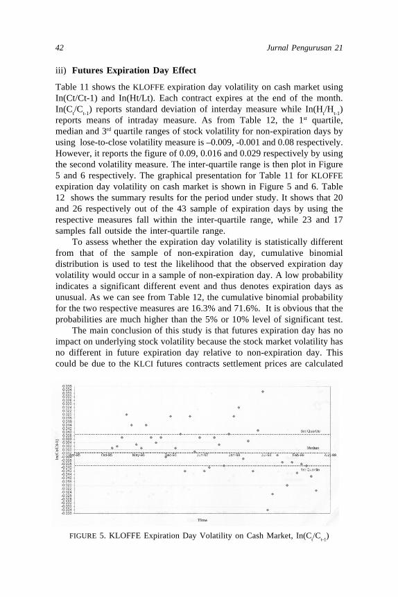
reports means of intraday measure. As from Table 12, the 1st quartile,median and 3rd quartile ranges of stock volatility for non-expiration days byusing lose-to-close volatility measure is –0.009, -0.001 and 0.08 respectively.However, it reports the figure of 0.09, 0.016 and 0.029 respectively by usingthe second volatility measure. The inter-quartile range is then plot in Figure5 and 6 respectively. The graphical presentation for Table 11 for KLOFFEexpiration day volatility on cash market is shown in Figure 5 and 6. Table12 shows the summary results for the period under study. It shows that 20and 26 respectively out of the 43 sample of expiration days by using therespective measures fall within the inter-quartile range, while 23 and 17samples fall outside the inter-quartile range.

To assess whether the expiration day volatility is statistically differentfrom that of the sample of non-expiration day, cumulative binomialdistribution is used to test the likelihood that the observed expiration dayvolatility would occur in a sample of non-expiration day. A low probabilityindicates a significant different event and thus denotes expiration days asunusual. As we can see from Table 12, the cumulative binomial probabilityfor the two respective measures are 16.3% and 71.6%. It is obvious that theprobabilities are much higher than the 5% or 10% level of significant test.

The main conclusion of this study is that futures expiration day has noimpact on underlying stock volatility because the stock market volatility hasno different in future expiration day relative to non-expiration day. Thiscould be due to the KLCI futures contracts settlement prices are calculated

FIGURE 5. KLOFFE Expiration Day Volatility on Cash Market, In(Ct/C

t-1)


TABLE 11. KLCI Futures Expiration Day Volatility on Cash Market

Contract Month In(Ct/Ct-1) In(Ht/Lt)

1 Dec-95 0.001 0.006 2 Jan-96 0.002 0.011 3 Feb-96 0.007 0.007 4 Mar-96 0.02 0.007 5 Apr-96 0.014 0.014 6 May-96 0.003 0.007 7 Jun-96 0.001 0.011 8 Jul-96 0.014 0.015 9 Aug-96 0.007 0.01210 Sep-96 0.004 0.00511 Oct-96 0.007 0.00612 Nov-96 -0.004 0.0113 Dec-96 0.019 0.01914 Jan-97 0.001 0.00715 Feb-97 0.009 0.00916 Mac-97 -0.012 0.01917 Apr-97 0.019 0.01918 May-97 -0.001 0.00919 Jun-97 0.007 0.00820 Jul-97 -0.012 0.01521 Aug-97 -0.01 0.04422 Sep-97 0.007 0.01723 Oct-97 0.003 0.03224 Nov-97 -0.009 0.05125 Dec-97 0.009 0.02626 Jan-98 0.019 0.01927 Feb-98 0.024 0.01728 Mac-98 -0.005 0.01229 Apr-98 0.005 0.01430 May-98 -0.012 0.02231 Jun-98 0.011 0.02132 Jul-98 0.033 0.03333 Aug-98 -0.034 0.02434 Sep-98 -0.025 0.0235 Oct-98 -0.003 0.00936 Nov-98 -0.007 0.0337 Dec-98 -0.02 0.0538 Jan-99 -0.007 0.01939 Feb-99 -0.013 0.01640 Mac-99 0.008 0.02541 Apr-99 0.009 0.01542 May-99 -0.015 0.01543 Jun-99 -0.023 0.026


TABLE 12. Summary Results of Expiration Day Effect

In(Ct/Ct-1) In(Ht/Lt)

Interquartile Range1st Quartile -0.009 0.009Median -0.001 0.0163rd Quartile 0.008 0.029

Expiration daysInside IQR 20 26Outside IQR 23 17

43 43

Non Expiration days 830 830Total 873 873

Probability 16.3% 71.6%

FIGURE 6. KLOFFE Expiration Day Volatility on Cash Market, In(Ht/L

t)

based on the average value of the stock index for the last half hour of thetrading, that is from 4.45pm to 5.15pm. This determination of settlementprice is quite different from the Nikkei or FTSE 100. Lastly, the resultreported is consistent with the studies conducted in other countries such asby Stoll and Whaley (1987), Karakullukcu (1992), and Bacha and Villa(1993).


(iv) Futures Mispricing

a) Without Transaction Cost

Table 13 shows the summary results of average daily mispricing for eachcontract month for the period under study with no transaction cost. The tablealso reports overall mispricing, being the average of under and overpricing.It also shows that 25 of the 43 contracts studied had mean underpricing ofwhich 16 were significant. On the other hand, only 17 contracts had meanoverpricing and 9 were significant. The standard deviation of mispricingshows a steady increase over the later contracts. The mispricing is graphedand presented in Figure 7.

From the above observation, three conclusions can be drawn. First,there appears to be much more frequent underpricing than overpricing forthe period before crisis. Second, the percentage and magnitude of underpricingis larger. Overpricing appears to be of a lower magnitude. Third, thereappears to be stretches of very little or no overpricing (i.e. March toSeptember 1996). The result also shows mispricing is larger in the laterperiod of the study. This contradict with the findings of Brenner et al. (1989)and Bacha and Fremault (1993) which shows reduced mispricing over time.If one ignored the currency crisis starting from July 1997, there is clearly nodeclining trend in mispricing over the one and the half year period beforecrisis. Table 14 shows the breakdown of mean underpricing and overpricingwith the number of days on which underpricing and overpricing. The earlierobservation of higher frequency of underpricing before currency crisis isexplained and summarised in Table 15.

FIGURE 7. Daily Mispricing at KLCI Futures (Without Transaction Cost)


TABLE 13. Daily Mispricing Summary Statistics

Contract Observation No. Mean (%) Significant SD (%)

1 Dec-95 10 0.11 0.26 2 Jan-96 23 0.09 0.34 3 Feb-96 15 0.53 * 0.52 4 Mac-96 21 -0.08 0.29 5 Apr-96 21 -0.39 * 0.3 6 May-96 20 -0.3 * 0.42 7 Jun-96 20 -0.73 * 0.37 8 Jul-96 22 -0.5 * 0.33 9 Aug-96 22 -0.92 * 0.5310 Sep-96 21 -0.43 * 0.5611 Oct-96 23 0.11 0.3212 Nov-96 20 0.22 * 0.3913 Dec-96 21 -0.07 0.514 Jan-97 22 -0.21 0.715 Feb-97 16 0.19 0.5516 Mar-97 21 -0.31 0.7217 Apr-97 21 -0.99 * 1.5718 May-97 19 -0.56 2.5419 Jun-97 21 -0.67 1.5120 Jul-97 22 -1.44 * 2.1521 Aug-97 21 -3.51 * 4.3222 Sep-97 21 -3.08 * 6.6723 Oct-97 22 -2.74 * 5.224 Nov-97 20 -3.54 * 5.0725 Dec-97 22 0.32 6.9226 Jan-98 17 1.68 9.727 Feb-98 19 -0.25 4.2728 Mar-98 22 -0.97 3.4829 Apr-98 20 -4.45 * 2.6530 May-98 19 -3.85 * 4.331 Jun-98 22 -1.3 4.5132 Jul-98 22 -2.07 * 3.7133 Aug-98 20 -3.56 * 5.8334 Sep-98 21 6.53 17.5635 Oct-98 21 3.95 * 4.1736 Nov-98 21 4.17 * 2.8637 Dec-98 22 3.23 * 1.8938 Jan-99 16 2.67 * 3.6339 Feb-99 17 -0.3 3.9440 Mar-99 22 0.54 3.5941 Apr-99 22 4.62 * 2.8742 May-99 21 1.57 * 2.1943 Jun-99 22 1.53 * 1.21

*indicates that mispricing is significantly different from 0 using t-test at 10% level


TABLE 14. Daily Mispricing Without Transaction Cost

Underpricing (Mt<0) Overpricing (Mt>0)Contract Observation No. days Mean (%) No.days Mean (%)

No.

Dec-95 10 5 -0.1 * 5 0.33 *Jan-96 23 8 -0.27 * 15 0.25 *Feb-96 15 3 -0.13 12 0.77 *Mar-96 21 15 -0.25 * 6 0.28 *Apr-96 21 19 -0.4 * 2 0.07May-96 20 14 -0.53 * 6 0.21 *Jun-96 20 19 -0.77 * 1 0.3 *Jul-96 22 20 -0.55 * 2 0.08 *Aug-96 22 21 -0.96 * 1 0.04Sep-96 21 15 -0.69 * 6 0.21 *Oct-96 23 9 -0.22 * 14 0.33 *Nov-96 20 5 -0.17 * 15 0.35 *Dec-96 21 12 -0.39 * 9 0.36 *Jan-97 22 15 -0.63 * 7 0.58 *Feb-97 16 6 -0.36 * 10 0.52 *Mac-97 21 14 -0.7 * 7 0.48 *Apr-97 21 15 -1.86 * 6 1.2 *May-97 19 10 -2.57 * 9 1.45 *Jun-97 21 16 -1.26 * 5 1.21 *Jul-97 22 16 -2.49 * 6 1.35 *Aug-97 21 17 -4.99 * 4 2.81 *Sep-97 21 14 -6.73 * 7 4.21 *Oct-97 22 16 -4.1 * 6 4.22 *Nov-97 20 15 -5.76 * 5 3.12 *Dec-97 22 10 -5.86 * 12 5.48 *Jan-98 17 9 -5.48 * 8 9.74 *Feb-98 19 11 -3.02 * 8 3.56 *Mac-98 22 13 -2.97 * 9 1.93 *Apr-98 20 19 -4.69 * 1 0.19May-98 19 16 -5.22 * 3 3.47Jun-98 22 15 -3.71 * 7 3.85 *Jul-98 22 16 -3.91 * 6 2.83 *Aug-98 20 16 -6.05 * 4 6.39 *Sep-98 21 7 -4.38 * 14 11.99 *Oct-98 21 6 -1.32 * 15 6.06 *Nov-98 21 2 -0.39 * 19 4.66 *Dec-98 22 1 -0.5 * 21 3.41 *Jan-99 16 4 -1.54 * 12 4.42 *Feb-99 17 9 -3.33 * 8 2.72 *Mar-99 22 13 -1.56 * 9 3.57 *Apr-99 22 1 -0.77 * 21 4.88 *May-99 21 5 -1.04 * 16 2.44 *Jun-99 22 1 -0.54 * 21 1.63 *

873 493 380

*indicates mispricing is significant at 10% level.


We can see obviously that 64% (256 out of 400 days) of the observedmispricing was negative. This is in contrast to the early research by Yau etal. (1990) on S&P 500 futures contract whose prices were constantly at apremium. The average size of the negative mispricing, -0.86% of the spotindex is greater than that of the positive mispricing, 0.56%. Similarly thestandard deviation of the negative mispricing is higher than that of thepositive (0.94% versus 0.60%). Extreme overpricing did happen, though notfrequently. It is observed that most of the positive mispricing are clusteredaround five months: January and February 1996, October and November1996, and February 1997.

b) With Transaction Costs

Table 16 shows the mean over and underpricing with transaction costs withthe number of days of overpricing and underpricing as defined by M

t. The

mean is calculated for the days on which underpricing and overpricing waslarge enough to violate the transaction cost upper and lower bounds. Figure

TABLE 15. Futures Mispricing from 15/12/95 to 31/7/97

Underpricing Overpricing

Overall mean -0.86 0.56Overall standard deviation 0.94 0.60Observation no. (400) 256 144

FIGURE 8. Daily Mispricing at KLCI Futures (With Transaction Cost)


10231521212020222221232021221621211921222121222022171922201922222021212122161722222122873

0000001073000102139713171314151086717141115166300367020246

0.000.000.000.000.000.00-0.020.00-0.25-0.180.000.000.00-0.050.00-0.44-0.82-2.02-1.16-1.68-3.84-6.03-3.88-4.62-4.71-4.99-3.90-3.73-3.77-4.42-3.69-3.00-4.91-3.90-0.670.000.00-1.05-3.07-1.230.00-0.870.00

*

******************

*

*

Dec 95Jan-96Feb-96Mar-96Apr-96May-96Jun-96Jul-96Aug-96Sep-96Oct-96Nov-96Dec-96Jan-97Feb-97Mar-97Apr-97May-97Jun-97Jul-97Aug-97Sep-97Oct-97Nov-97Dec-97Jan-98Feb-98Mar-98Apr-98May-98Jun-98Jul-98Aug-98Sep-98Oct-98Nov-98Dec-98Jan-99Feb-99Mar-99Apr-99May-99Jun-99

TABLE 16. Daily Mispricing With Transaction Cost

Contract Observation Underpricing (Mt<0) Overpricing (M

t>0)

No. No. days Mean(%) No. days Mean(%)

0020000000000000353246541067603554111518211056201212210

indicates mispricing is significant at 10% level

*

*

***

**

**********

0.000.000.180.000.000.000.000.000.000.000.000.000.000.000.000.000.601.120.591.002.303.644.302.055.2111.512.881.650.002.343.342.265.2313.844.913.742.284.092.924.053.941.781.32


8 shows the graph of daily mispricing with transaction of KLCI Futures. Oneobvious observation is that positive mispricing have disappeared up toMarch 1997 except for one contract month of February 1996. This is dueto the fact that before the transaction costs, the magnitude of positivemispricing was not large. The average size of the positive mispricing isabout 0.44% of the spot index. With a transaction costs of 1.11%, all of thepositive mispricing were considered within bounds up to March 1997 (i.e.the futures contract were priced fairly according to the cost of carry model).However, 246 cases of negative mispricing remained after the transactioncosts. In addition, majority of the mispricing for April 1997 to September1998 contracts still experienced negative mispricing even after the transactioncosts. However, September 1998 to June 1999 contracts was overvaluedmost of the time.

CONCLUSIONS AND RECOMMENDATIONS

In this section, summary, concluding remarks, limitation of the research,implications and suggestions for additional research are discussed.

i) Impact of Futures Trading On Its Underlying Stocks

The main conclusion of this study is that the introduction of financial futurestrading has not destabilized cash markets. Both the day to day and intra-dayprice volatility of the stock and futures markets over the seven year periodfrom 1992 to 1999 were examined. No evidence was found which linksfuture trading to an increase in general market volatility. If anything, the oneand the half years period following the futures introduction had lowered thevolatility. However, this may be due to the currency crisis.

In this study, we also provide an empirical investigation of the volatilityof 100 component stocks in KLSE CI and non KLSE CI before and after theKLSE CI futures introduction and we find evidence of decrease in volatility.Seven industry sectors in KLSE CI have declined in volatility (8.40%)whereas its corresponding matched group shows an increase of 71.80% inthe post compared to the pre-futures period. At the significant level of a =0.05 and 0.10, the decrease in volatility of KLSE CI group are 23.10% and22.20% respectively compared to its corresponding matched group, whichshows an increase by 20.20% and 15.30% respectively.

Fifty-three stocks have decreased in volatility in the 2nd post-futuresperiod compared to only 24 stocks in the 1st post-futures period. In the 1st

post-futures period, KLSE CI sample shows slight increase in volatility, butin the 2nd post-futures period, it shows a decrease of 20%. This might be dueto relatively more active trading in the futures market sometimes after fromthe introduction date. An increase in involvement of market participants


tends to stabilize the underlying spot market and subsequently reduces thevolatility.

KLSE CI Futures trading might decrease its underlying stock pricevolatility by three reasons. It increases information flow, increases marketliquidity and provides hedging opportunities. The existence of futurestrading in a market should increase the speed with which information isdisseminated, the area over which it is disseminated and the degree ofsaturation within the area. It should tend to equalize the flows of informationto current and potential futures and cash market participants. Therefore, thedecrease in volatility of KLSE CI underlying stocks could be due to theimprovement in the information flows fostered by the KLSE CI Futurestrading.

In this study, we are dealing with the stock price volatility where thefluctuations of the stock prices might be due to both internal (firm-specificcharacteristics) and external factors (economic, technological, political andlegal), which are not predictable, therefore, this study might involve variouspractical difficulties that cannot be completely resolved. To isolate theunrequired volatility, this study has constructed a sample of matching stocksas group and chose a short test period to minimize the time variation ofstock price. The matching of the stocks might not be perfect due to the smallnumber of stocks available for matching.

The volatility of financial markets has become increasingly importantfor market participants, regulators and academicians. Innovations in thefinancial products offered to the market have increased the complexity of thefinancial environment. Some of these recent innovations such as financialderivative securities have received considerable media attention. Marketparticipants are keen to know whether this kind of innovations will have anyimpact to the markets especially for their underlying stocks to enable themto make an economic profit in this complex market.

From this study, it shows that the trading in futures market willeventually reduce the volatility of its underlying stocks. An increase in awell-informed speculative trading may decrease the volatility and increaseliquidity because informed traders provide liquidity in such events (Harris,1989).

The results are important for the regulators and markets, especially theKLSE and KLOFFE, because the evidence is inconsistent with the publicperception that derivatives increase risk. At the same time, these results areimportant to the academicians who seek to understand more on howderivative securities may be related to financial risk. Besides, the researchresults provide a general reference for those market participants who wouldbenefit from understanding the relationship of price volatility behaviorbetween the futures trading and its underlying stocks. This is particularlyimportant for those investors and speculators who are continuously seeking


for better ways of estimating the volatility of underlying stocks. Forportfolio managers, they might be able to perform better planning andimplementation of their investment decision and better selection of investmentportfolio with the guideline of this research.

To further test the hypothesis developed in this research, more studiesneed to be conducted on a wider range of periods and with different modelsuch as GARCH. Looking at a trading range alone is insufficient because ittakes no account of price fluctuations between the high and the low, whilevariance around a long run mean could be misleading when prices containa trend. GARCH models are appropriate to be of used since they are capableof capturing the three most empirical features observed in stock return data:leptokurtosis, skewness and volatility clustering (Taufiq 1996).

ii) Relative Volatility Between Futures And Stock Markets

Inter-market comparison shows futures market volatility is higher. Theconclusions are the same when volatility is measured by both method. Theresult is consistent with earlier studies in other countries.

The interpretation for the higher futures volatility are (i) “noise traders”are more active in the futures market, so temporary price swings areexaggerated by Black (1986). (ii) The future contract prices react morequickly to new information because the contract has lower transaction costsand (iii) they price the bundle of underlying stock simultaneously. Amihudand Mendelson (1989) conclude that both these explanations contribute tothe higher volatility of futures returns.


The test shows no evidence of increase stock market volatility on futuresexpiration days. This could be due to the KLCI futures contracts settlementprices are calculated based on the average value of the stock index for thelast half hour of the trading, that is from 4.45pm to 5.15pm. This isconsistent with studied conducted by Bacha and Villa (1993), Stoll andWhaley (1987) and Karakullukcu (1992).

The size of the futures market is estimated to be 25% of the stockmarket Ringgit volume. The relative size is still small and not significant.So, the no evidence of an expiration day effect should not be surprisinggiven the perspective of size.

iv) Futures Mispricing

The test of the mispricing shows frequent mispricing. There appears to bemuch more underpricing (64%) than overpricing before the start of financialcrisis. This is in contrast to the early research by Yau et.al (1990) on


S&P500 futures contract whose prices were constantly at a premium.Furthermore, overpricing appears to be of a lower magnitude. There appearsto be stretches of very little or no overpricing (i.e. March to September1996). The result also shows mispricing is larger in the later period of thestudy. This contradict with the findings by Brenner et al. (1989) and Bachaand Fremault (1993) which show reduced mispricing over time. If oneignored the currency crisis starting from July 1997, there clearly is nodeclining trend in mispricing over the one and the half year period beforecrisis. If transaction cost is taken into accounts, the result exhibit lessmispricing.

While transaction costs would affect arbitrageable opportunities on bothover and underpricing. We believe that this has partly to do with theregulatory framework. In essence, the regulation is biased against ReverseCash and Carry arbitrage. In Malaysia, short selling is prohibited. When acontract is underpriced, the index arbitrage strategy would be to long futuresand short the underlying stocks, but the regulatory framework is against this.However, when futures are overpriced, there is no regulations preventingwhosoever to go short futures and long stocks. We believe the short sellingregulation is the major reason for the underpricing.

REFERENCES

Abhay, H.A. 1998. Linear and nonlinear Granger causality: Evidence from the UKStock Index Futures Markets. The Journal of Future Markets 18(5): 519-540.

Amihud, Y. & Mendelson, H. 1989. Index and index future returns. Journal ofAccounting, Auditing and Finance.

Arditti, F.D., Ayaydin, S., Muttu, R.K. & Rigsbee, S. 1986. A Passive FuturesStrategy That Outperforms Active Management. Financial Analyst Journal 42:63-67.

Bacha, O. & Villa, F. 1993. Multi-market trading and price-volume relationship: Thecase of the Nikkei stock index futures markets. The Journal of InternationalFinancial Markets, Institutions and Money 6(1).

Billingsley, R.S. & Chance, D.M. 1988. Options market efficiency and the boxspread strategy. The Financial Review 20 (4): 287-301.

Bhatt, S. & Cakici, N. 1990. Premiums on the stock index futures: Some evidence.The Journal of Futures Markets 10 : 367-375.

Brenner, M., Subrahmanyam, M.G. & Uno, J. 1989. The behavior of prices in theNikkei spot and futures market. Journal of Financial Economics 46 (2): 363-383.

Brenner, M., Subrahmanyam, M.G. & Uno, J. 1990. Arbitrage opportunities in theJapanese stock and futures markets. Financial Analysts Journal 46: 14-24.

Black, F. 1976. The pricing of commodity contracts. Journal of Financial Economics3: 167-179.

Black, F. 1986. Noise. Journal of Finance 41: 529-544.Chan, K., Chan, K.C. & Karolyi, G.A. 1991. Intraday volatility in the stock index

and stock index futures markets. Review of Financial Studies 4: 657-684.


Choi, H. & Subrahmanyam, A. 1994. Using intraday data to test for effects of indexfutures on the underlying stock market. Journal of Futures Markets 14 (3):293-322.

Choudhry, T. 1996. Stock market volatility and the crash of 1987: Evidence from sixEmerging Markets. Journal Of International Money and Finance 15 (6): 969-981.

Cutter, D.M., Poterba, J.M. & Summers, L.H. 1989. What moves stock prices?Journal of Portfolio Management 15: 4-12.

Edwards, F.R. 1988a. Does futures trading increase stock market volatility? FinancialAnalysts Journal 44: 63-69.

Edwards, F.R. 1988b. Futures Trading and cash market volatility: stock index andinterest rate futures. Journal of Futures Markets 8(4): 421-439.

Fauzias, Mat Nor & Liew Ah Heng. 1996. Examining the relationship betweenKLCI futures prices and its futures spot index: A preliminary study. A paperpresented at Seminar Kebangsaan Perdagangan dan Alam Sekitar, UniversitiKebansaan Malaysia. 14-15 Mei, 1996.

Figlewski, S. 1984. Explaining the early discounts on the stock index futures: Thecase for disequilibrium. Financial Analyst Journal 40: 43-47.

Freris, A.F. 1990. The Effects of the introduction of stock index futures on stockprices: The experience of Hong Kong 1984-1987. Pacific Basin CapitalResearch: 409-416.

Hancock, G.D. 1991. Future options expirations and volatility in the stock indexfuture market. Journal of Future Markets 11 (3): 319-330.

Harris, L. 1989. S&P 500 cash stock price volatilities. Journal of Finance 44: 1155-1175.

Hodgson, A. & Nicholls, D. 1991. The impact of index futures market on Australiashare market volatility. Journal of Business Finance and Accounting 18: 267-280.

Ibrahim, A.J, Othman, K and Bacha, O.I. 1999. (Title) Capital Market Review (7)1& 2: 1-46.

Investor’s Digest. December 1995 to June 1999.KLOFFE website. www.kloffe.com.my/oview.htm.Karakullukcu, M. 1992. Index Futures: Expiration day effects in the UK and

prospects in Turkey, Mimoe, London School of Economics: 36Klemkosky, R.C. & Lee, J. H. 1991. The intraday ex-post and ex-ante profitability

of index arbitrage. The Journal of Futures Markets 11: 291-311.Kok, K. L. 1992. Construction on stock index futures. 26th and 27th February 1992,

Subang Jaya, Holiday Villa, Kuala Lumpur: University Of Malaya.Koutmas, G. & Tucker, M. 1996. Temporal relationship and dynamic interactions

between spot and futures stock markets. Journal of Futures Markets 16: 55-69.Kipnis, G.M. & Tsang, S. 1984. Arbitrage in stock index futures. In …… eds. F.J.

Fabozzi & G.M. Kipnis, 124-141. ………..Dow-Jones Irwin.Kyle, A.S. 1985. Continuous auctions and insider trading. Econometrica 53: 1315-

1335.Lee, S.B. & Ohk, K.Y. 1992. Stock index futures listing structural change in time

varying volatility. Journal of Futures Markets 12: 493-509.Miller, M.H. 1990. International competitiveness of US futures exchanges. Journal

of Financial Services Research 4: 387-408.


Miller, M.H. 1995. Financial innovations and market volatility. Cambridge: BlackwellPublishers.

Miller, M.J. & Galloway T.M. 1997. Index futures trading and stock return volatility:evidence from the introduction of Midcap 400 index futures. The FinancialReview 32: 845-866.

Parkinson, M. 1980. The extreme value method for estimating the variance of thereturn. Journal of Business 53: 61-65.

Pericli, A. & Koutmas, G. 1997. Index futures and options market volatility. Journalof Futures markets 17 (8): 957-974.

Powers, M. J. 1970. Does futures trading reduce price fluctuations in the cashmarkets. American Economic Review 60: 460-464.

Powers, M. J. 1993. Starting out in futures trading. Chicago, IL: Probus PublishingCo.

Randall, T., Fortenbery & Hector, O.Z. 1997. An evaluation of price linkagesbetween futures and cash markets for cheddar cheese. Journal of FuturesMarkets 17 (3): 279-301.

Samuelson, P. 1965. Proof that properly anticipated prices fluctuate randomly.Industrial Management Review 6: 41-49.

Santoni, G.J. 1987. Has program trading made Stock prices more volatile? Reviewof Federal Reserve Bank of St. Louis: 18-29.

Sato, M. 1991. Impact of the futures market on the stock market. Pacific BasinCapital Markets Research.

Schwert, G. W.1990. Stock market volatility. Financial Analysts Journal 46: 23-345.Simon & Schuster. 1998. SPSS 8.0 for Windows Brief Guide. USA: Prentice Hall.Stoll, H.R. & Whaley, R.E. 1987. Program trading and expiration day effects.

Financial Analysts Journal. March/April 1987.Stoll, H.R. & Whaley, R.E. 1990. The Dynamics of stock index and stock index

futures returns. Journal of Financial and Quantitative Analysis 4: 441-468Stoll, H.R. & Whaley, R.E. 1991. Expiration day effects: What has changed?

Financial Analysts Journal 47: 58-72.Stuart, A. & Ord, J.K. 1987. Kendall’s advanced theory of statistics (5th ed.).

London: Griffen Books.Subrahmanyam, A. 1991. Risk aversion, market liquidity and price efficiency.

Review of Financial Studies 4: 417-441.Tan, T.H. 1996. Corporate Handbook: Malaysia. Singapore Thomson Information

(S.E. Asia): xii-xxxi.Tay. 1991. Firm size and January effects in the KLSE. Malaysian Management

Review 26 (2): 24-34.Yau, J., Schneeweis, T. & Yung, K. 1990. The behaviour of stock index futures in

Hong Kong: before and after the crash. Pacific Basin Capital Markets Research:357-377.

Yadav, P.K. & Pope, P.F. 1990. Stock index futures arbitrage: International evidence.Journal of Futures Markets 10 (6): 573-603.

Department of FinanceFaculty of Business ManagementUniversiti Kebangsaan Malaysia43600 UKM, Bangi, Selangor D.EMalaysia.

volatility, expiration day effect and pricing efficiency...

Documents