volatility-price relationships in power exchanges
TRANSCRIPT


Volatility-price relationships in power exchanges:
A demand-supply analysis∗
Sandro Sapio†
April 1, 2008
Abstract
The evidence of volatility-price dependence observed in previous works (Karakatsaniand Bunn 2004; Bottazzi, Sapio and Secchi 2005; Simonsen 2005) suggests that thereis more to volatility than simply spikes. Volatility is found to be positively correlatedwith the lagged price level in settings where market power is likely to be particularlystrong (UK on-peak sessions, the CalPX). Negative correlation is instead observed inmarkets considered to be fairly competitive, such as the NordPool. Prompted by theseobservations, this paper aims to understand whether volatility-price patterns can bemapped into different degrees of market competition, as the evidence seems to suggest.
Price fluctuations are modelled as the outcome of dynamics in both sides of the market- demand and supply, which in turn respond to shocks to the underlying preferenceand technology fundamentals. Negative volatility-price dependence arises if the marketdynamics is accounted for by common shocks which affect valuations uniformly. Positivedependence is related to the impact of asymmetric shocks. The paper shows that undercertain conditions, these volatility-price patterns can be used to identify the exercise ofmarket power. Identification is however ruled out if all shocks affect valuations uniformly.
JEL Classifications: C16, D4, L94.Keywords: Electricity, Market, Volatility, Supply Curve, Demand Curve, Funda-
mentals, Shocks.
1 Introduction
Among the goals of the power industry restructuring, attaining a high degree of efficiency isviewed as a primary one. Widespread demand for lower energy prices urged regulators tointroduce market-based trading in key segments of the industry, such as electricity production(Joskow 1996, Newbery 2002). Whether markets have been successful in yielding lower powerprices is still a debated issue. Much better established is the evidence that liberalized powerexchanges can be extremely volatile. Simonsen (2005) reports a 16% value for the annualizedvolatility of NordPool daily returns - a value much higher than for other energy markets,such as coal, natural gas, and petroleum (Schwartz and Smith 2000). Sharp and short-livedspikes are commonly observed in market sessions characterized by a very tight balance between
∗Preliminary draft: please, do not quote without permission.†Department of Economic Studies, University of Naples Parthenope, and LEM, Sant’Anna School of Ad-
vanced Studies, Pisa. E-mail: [email protected]
1

demand and the available generating capacity. Besides, power exchange volatility has beenshown to possess a rich temporal structure, which has been analyzed through reduced-formmodels, such as GARCH, regime-switching, and jump-diffusion models (see Weron 2007 fora survey). Further statistical studies have shed light on patterns of correlation between thelagged electricity price level and measures of volatility. Karakatsani and Bunn (2004) fitted apower law on the relationship between the lagged price level and the residual volatility of theprice model, and observed various patterns across hours in the UK market. Bottazzi, Sapioand Secchi (2005) and Simonsen (2005) observed negative correlation for the NordPool market;Sapio (2005, 2008) and Bottazzi and Sapio (2008) described positive correlation betweenvolatility and the price level in the APX and CalPX, as well as regime breaks in NordPooland Powernext. These patterns seem to be somewhat related to different degrees of marketcompetition. Positive correlation in the UK is observed on-peak, when the demand-capacityratio is very high, and in a market, such as the CalPX, which is widely recognized as probablythe most striking example of how market power can lead to the collapse of a trade institution(Joskow 2001, Wolak 2003). Negative correlation is instead found in the NordPool, whichheavy reliance on hydropower suggests it may be fairly competitive. If such association findsa theoretical foundation, the volatility-price patterns can be seen as “footprints” left by powerproducers who exercise market power.
Analyzing the mechanisms which give rise to volatility-price patterns is appealing for thisreason, but not only. Making sense of volatility patterns can improve our understanding ofpossible trade-offs between two key goals of energy policy: ensuring low and stable prices. Suchknowledge can be precious to discipline policy-making, by clarifying the menu of the attainablepolicy results. Moreover, accurate modelling of the time structure of volatility enables moreprecise market forecasts (Weron 2006). As such, it can foster the design of efficient tools forrisk management, a key step on the way to the long-term achievement of liquid and robustpower exchanges (Powell 1993).
The paper seeks to explain the emergence of volatility-price patterns in power exchanges,and to understand whether volatility patterns can be mapped into different degrees of compe-tition, and hence used to identify anti-competitive behaviors.. The analysis is carried out bymeans of a structural approach, based on direct modelling of the demand and supply curves.The basic insight behind this approach is that price fluctuations are due to dynamics in bothsides of the market - demand and supply. These are in turn responsive to changes in technol-ogy and preference fundamentals, such as the demand responsiveness to price signals and thestructure of production costs.
Among the advantages of using a structural approach, it allows to map the evidence intospecific features of the market curves. The properties of demand and supply curves conveyrelevant information as to the degree of market competition and transparency. For instance, alow value of the price-elasticity of demand is a source of market power. Further, if the supplycurve lies above the marginal cost curve and is steeper, this is due to market power abuse bymulti-plant power generating companies (Ausubel and Cramton 1996). In addition to this, andimportantly, the design of any policy measure to mitigate volatility needs to outline batteriesof incentives which directly touch on consumption habits and investment plans. Knowledgeof the main sources of volatility is critical, in that the required policy actions may differdramatically whether volatility is due to demand or supply factors.
Results from this paper reveal that negative volatility-price dependence takes place ifthe bulk of market dynamics is due to uniform shocks, i.e. common shocks whose impacton valuations is uniform across agents. The reason is that, if all valuations on either sideof the market change by the same amount, the shock weighs proportionally more on low
2
valuations, which are the marginal ones when the price is low. Positive price dependence isa sign that asymmetric shocks are the main volatility drivers. These shocks typically affectthe degree of heterogeneity among commodity valuations. Under certain conditions, theirimpact is amplified by the price level. As the main implications for competition policy, theidentification of market power by means of volatility-price patterns requires the occurrence ofasymmetric shocks. Indeed, if all shocks affect valuations uniformly, volatility patterns do notvary across market regimes. Since markets with only uniform shocks are hard to imagine, theassociation between volatility-price patterns and competition suggested by the evidence mighthave some foundation.
This paper fills a gap in the existing theoretical literature on the volatility of power ex-changes. Some previous works place a similar emphasis on the role of market structure in ex-plaining volatility. Mount (2000) posits a perfectly inelastic demand and a constant-elasticitysupply function. As shown, the market-clearing price is more volatile, the lower the supplyelasticity. However, agents behaviors are not explicitly modelled. While the analysis in thepresent paper eschews modelling behaviors too, it is general enough as to include several op-timizing models as special cases. Mount (1998) proposes a Cournot model with displacedquadratic cost functions, and demonstrates that volatility is higher in an oligopolistic settingthan under perfect competition, in that market power makes the supply curve more inelas-tic. Yet, no account is given for the volatility-price patterns observed more recently. Barlow(2002) and De Sanctis and Mari (2007) assume a stochastically varying demand function, andaim to account for the emergences of spikes. Kanamura’s (2007) paper on the natural gasmarket is another valuable attempt within the structural approach, but its goal is to explainthe evidence of inverse leverage effects.
The paper is structured as follows. Section 2 reviews the main facts on the volatility ofpower exchanges, with a major focus on volatility-price patterns. Section 3 describes therole of fundamentals in driving market dynamics, and offers some definitions and taxonomies.Section 4 breaks down volatility into components associated to single fundamental drivers,gives a flavour of the possible patterns, and illustrates some examples. In Section 5, the linkagebetween price dependence patterns and the properties of market curves is investigated, whileSection 6 proposes some market power implications. Discussion and conclusions are in Section7.
2 Evidence on the volatility of power exchanges
The volatility of electricity markets is commonly associated with the existence of significantrigidities on both the demand and the supply sides of the market (cf. Alvarado and Rajaraman2000, Stoft 2006). First, there exists wide evidence of short-run demand inelasticity: Considine(1999), Halseth (1999) and Earle (2000) report estimated values between 0.05 and 0.5. Thisis partly related to electricity being a necessary consumption good and production input inseveral economic activities, and partly to the fact that the short-run dynamics of the retailprice is not affected by wholesale price movements, due to lack of metering. Second, powersupply is subjected to capacity constraints, ramp rates, fixed and quasi-fixed costs. Thesetechnical constraints require a certain amount of base-load power to be supplied inelastically.1
The analysis of volatility in power exchanges has benefited from up-to-date statistical andeconometric techniques (Bunn 2004). A very common approach in the relevant literature deals
1In their study on the Spanish market Omel, Guerci et al. (2005) have documented that a fraction of powersuppliers (passive sellers) offer their capacity at a zero ask price.
3

with various versions of the GARCH model, which entails the estimation of autoregressiveand moving average components of the conditional volatility of electricity prices. A cursoryreview of research in this field includes Bellini (2002), Worthington et al. (2002), Knitteland Roberts (2005), Cavallo, Sapio and Termini (2005), and Guerci et al. (2006). Theseworks, among the many, shed light on a few interesting empirical properties of power exchangevolatility, such as the existence of clustering patterns, persistence, mean-reversion, and theso-called inverse leverage effect - i.e. stochastic innovations have an asymmetric impact on thevolatility level, with positive shocks causing larger increases in volatility (Knittel and Roberts2005; Hadsell, Marathe and Shawky 2004). Some refinements of the existing econometrictechniques have been called upon in order to cope with the observed discontinuities in thetemporal behavior of electricity prices. The jump-diffusion process (Merton 1976) has receivedwidespread applications in studies on the power market: see the papers by Johnson and Barz(1999), Escribano et al. (2002), Villaplana (2004) and Knittel and Roberts (2005). As analternative way to capture the sudden shifts observed in electricity prices, the regime-switchingmodel (Hamilton 1989) posits the existence of multiple price regimes and aims to estimate theassociated switching probabilities. The jump-diffusion and the regime-switching approacheshave been merged in the works by Ethier and Mount (1998), Huisman and Mahieu (2003),Weron, Bierbrauer and Trueck (2004), Geman and Roncoroni (2006), and De Sanctis and Mari(2007), whose estimates reveal the dual nature of volatility - large probability to persist inany given state, along with extremely sizeable jumps due to transitions between states.
While these works provide satisfactory accounts of the time behavior of the volatility level,there are good reasons to expect that volatility is not homogeneous across price levels. Asan interesting clue to this, spikes are more likely when the load and prices are high (Mount2000). Closer to a demand-supply focus, demand is more elastic when prices soar: energyusers are induced to adopt energy saving habits, or to arbitrage between market segments,e.g. by rebalancing their portfolios. Hence, demand responsiveness may not be uniform.Sources of supply rigidity seem to apply differentially across price levels, too. At times ofhigh load, incentives exist for suppliers to withhold capacity in order to exploit the emergingprofit opportunities, making the supply responsiveness greater when price is high (see Harveyand Hogan 2001). Alternatively, power suppliers may choose to over-produce as a way tocause network congestion and therefore higher prices. Also, fixed and quasi-fixed costs havea stronger impact on average costs when the quantity traded is small, and so are prices. Itis however worth recalling circumstances in which the supply elasticity may actually displayan inverse relation with the price. First, in most power markets the supply stack has arapidly increasing slope, which implies a convex supply curve, as commonly observed. Second,a supplier with market power may be completely indifferent about having marginal unitsdispatched, as there is no penalty to the supplier of setting offers for marginal units at very highlevels (Ausubel and Cramton 1996; Mount, Ning and Oh 2000). This may give rise to a convexsupply function too. Finally, in systems based on a large share of hydropower production, wetwinters may cause the filling fraction of water reservoirs to reach maxima during the followingsummer and fall. In order to prevent the reservoirs from flooding, hydroelectric plants areready to produce at whatever low prices the market may determine (Simonsen 2005).
An empirical approach which seems better suited to understanding the varying impact ofrigidities on volatility was adopted by Karakatsani and Bunn (2004), Bottazzi, Sapio and Sec-chi (2005), and Simonsen (2005), who studied the relationship between measures of volatilityand the lagged price level. The former dealt with the UK power market. The latter twopapers, focused on the NordPool market, have been subsequently extended by Sapio (2005),Sapio (2008), and Bottazzi and Sapio (2008) to other markets, such as the CalPX, the Dutch
4

APX, and the French Powernext.Karakatsani and Bunn (2004) estimated a price model via GLS, including some of the
main fundamental variables of the electricity market as regressors, i.e. the demand leveland curvature, and the demand-capacity margin. The volatility of the model residuals ǫ wasmodelled as a power law of the lagged price level:
√
V [ǫt] = χpρt−1 (1)
Estimates of the power exponent for peak hours were positive, whereas estimation on off-peak hours yielded negative values. These patterns, as the authors suggested, could be dueto the fact that producers employ different bidding strategies and use different degrees of“arbitrariness” in their behaviors under different relative scarcity.
Simonsen (2005) computed daily logarithmic returns of NordPool wholesale day-aheadprices, sorted them in ascending price order, and after smoothing them through a medianfilter, fitted a stretched exponential plus a constant:
√
V [∆ log pt] = k0 + ek1pk2
t−1 (2)
where k0, k1 and k2 are costant parameters, V [.] the variance operator, and ∆ the firstdifference operator. The resulting estimates showed a negative price level dependence ofvolatility for the lowest prices, and a much milder dependence for higher prices. Interestingly,the gap between volatilities corresponding to the lowest and the highest price levels amountsto about an order of magnitude.
Bottazzi, Sapio and Secchi (2005), Sapio (2005), Sapio (2008) and Bottazzi and Sapio(2008) modelled the standard deviation of returns as a power function of the lagged pricelevel, after removing time dependencies from returns. Taking natural logarithms, this reads
√
V [∆ log pt] = χpρt−1 (3)
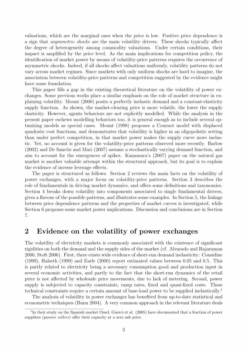
where χ and ρ are constant coefficients, ∆ log pt is a sequence of normalized log-returns.The parameter ρ tunes the type of volatility-price pattern. Estimation of the power lawscaling model is performed using a binning procedure.2 Results allow to detect two kindsof volatility-price dependence patterns: (i) monotonically decreasing, with a break beyond aprice threshold (NordPool, Powernext), (ii) monotonically increasing (CalPX, APX). Fig. 1depicts examples of the patterns observed.
These patterns seem to be associated to different degrees of market competition. Positivecorrelation is observed in cases when the market is likely to have been strongly affected bymarket power abuse (on-peak sessions in the UK; the CalPX). Negative correlation is insteadfound in the NordPool, which could be considered fairly competitive thanks to its high share ofhydropower, which makes it harder for producers to implement capacity withholding strategies.The research question thus arises as to whether increasing voaltility patterns can be univocallyassociated to imperfect competition, and decreasing patterns to perfect (or nearly perfect)markets.
2For any given time series, data were grouped into equipopulate bins. Next, sample standard deviations oflog-returns in each bin were computed, and the logarithm of the sample standard deviations was regressed ona constant and on the logarithm of the median price level within the corresponding bins.
5

3 Fundamentals, valuations, and shocks
A common way of assessing market performance - vis-a-vis social welfare - is by comparingthe quoted price to the underlying market fundamentals. This lies at the heart of e.g. themarket efficiency hypothesis in the analysis of financial markets: the price is (informationally)efficient if it includes all information regarding the economic value of the issuer company (seeLeroy 1989 for a survey). In commodity markets, the definition of fundamentals may change,depending on the physical characteristics of the commodity. Restructuring the power industryhas often been welcomed as a move towards greater transparency, which is but a way to shapethe wide-spread claim that market trading will drive prices down to the cost-based value ofelectrical power. The reference fundamental here is productive efficiency, and in a transparentmarket the level and variability of power prices closely track the underlying dynamics of inputprices. However, demand factors have a relevant role to play: power markets are structurallyconstrained to clear at all times, as storage is not economically viable. Hence, fluctuations indemand are not smoothed out.
A wider notion of fundamentals of an electricity market is thus the set of variables whichdefine the structure of the consumption and production decision problems, resulting in themarket curves. Fundamentals refer to both sides of the market, and accordingly can becategorized in demand fundamentals and supply fundamentals. Demand fundamentals have todo with consumer choice rooted in preferences and bounded by budget and time constraints.Supply fundamentals are instead linked to the technological parameters behind the productionchoices. Fundamentals are ultimately tied to the valuations of the commodity by users andproducers. As a simple way to visualize fundamentals, one can see them as the parameters ofdemand and supply curves. The location of market curves is indeed affected by the averagevalue of electricity to producers (marginal costs) and consumers (reservation prices). Slopestake up the heterogeneity of valuations across agents. For instance, steep supply stacks denotea wide source diversification among plants.
While the dynamics of a transparent power exchange tracks the evolution of fuel costs, moregenerally electricity prices reflect the fluctuations in both demand and supply fundamentaldrivers. Shocks to agent valuations modify the shape of the market curves, and the powerprice changes to ensure market clearing. The volatility of fundamental drivers is transmittedto power prices, more or less intensely depending on how sensitive is price to fundamentals.Relatedly, it will prove useful to operate a distinction between shocks to fundamentals. Someshocks affect energy valuations uniformly across sellers and purchasers. These types of commonshocks can be termed uniform shocks. Other shocks, asymmetric shocks, only hit individualsor groups of agents, thereby modifying the degree of heterogeneity among valuations; or theyare common shocks yielding heterogeneous individual impacts.
Uniform and asymmetric shocks may lead to different volatility outcomes. Shocks thataffect valuations uniformly have the same impact on demand and/or supply, regardless of theprice level. For example, suppose temperature increases, leading to greater use of air condi-tioning. If all energy users adjust their electricity consumption levels in the same extent, thedemand curve shifts, with no impact on its slope. Shocks that engender asymmetric responseamong companies or among users will instead change the curve slopes. Think of a positiveshock to the marginal cost of a rather inefficient plant: all other cost levels being unaffected,the slope of the supply curve increases. It is worth stressing that in such a case, shocksare amplified by the price level. This insight may be extremely relevant in understandingvolatility-price dependence patterns.
In line with the above, let us provide some definitions. A demand fundamental δ is a
6

non-price argument of the demand function D. A supply fundamental σ is a non-price argu-ment of the supply function S. Demand and supply functions are assumed continuous anddifferentiable.3 Formally, demand equals
D = D(p, δ, σ) (4)
with the standard assumption ∂D/∂p ≤ 0, while supply reads
S = S(p, δ, σ) (5)
with ∂S/∂p ≥ 0 as usual. Derivatives with respect to δ and σ are left unrestricted.Whenever a common shock affects agents uniformly, its impact on either supply or demand
is price-invariant:
∂2D
∂δ∂p=
∂2D
∂p∂δ= 0
∂2S
∂σ∂p=
∂2S
∂p∂σ= 0
An asymmetric shock response yields a price-dependent change in demand or supply:
∂2D
∂δ∂p=
∂2D
∂p∂δ6= 0
∂2S
∂σ∂p=
∂2S
∂p∂σ6= 0
Unlike in the standard analysis of market curves, demand and supply fundamentals aretreated as arguments of the demand and supply functions. More specifically, they are assumedto be random variables, driven by geometric random walks:
δ = δgδ δ = δgδ
where gδ ≈ iid(0, vδ), gσ ≈ iid(0, vσ), with gδ and gσ mutually independent.4 This assump-tion is useful for the sake of simplicity, as well as for its empirical relevance concerning thedynamics of fuel prices (see Serletis and Herbert 1999, Schwartz and Smith 2000, Asche et al.2003, Postali and Picchetti 2006).
4 Volatility break-down
It is tempting to try and reduce the volatility of power markets to a function of the volatilitiesof fuel prices, and furtherly try and disentangle the respective contributions. Yet, electricityprices vary over time in response to changes in other fundamentals too, e.g. demand partic-ipation, the level of water reservoirs, and so forth. Thus, more generally one would like tobreak down the volatility of power markets into individual components, imputable to each oneof the most relevant power fundamentals. Benini et al. (2002) have noted how volatility isdue to uncertainty in fundamental drivers. A simple framework for doing so is the following.
3The author is aware that results obtained using continuous market curves are generally not achievable bytaking the continuous limit of discrete curves. Von der Fehr and Harbord (1993) were among the first to showthis, using an auction-theoretic approach better suited to deal with the discrete curves observed in reality.However, continuous models, such as the Supply Function Equilibrium model, have offered rather accuratepredictions of electricity market outcomes (Baldick, Grant and Kahn 2004). Hence the choice of a continuousapproach - besides its analytical convenience.
4Time subscripts have been omitted for the sake of notational parsimony. Assuming zero means does notaffect the results on volatility.
7

Consider the demand and supply functions introduced in the previous section (Eq. 4 andEq. 5 respectively). Because power is not economically storable, supply and demand needto perfectly match at all times. Given a uniform price auction format, the market-clearingcondition is that the price p∗ ensures D(p∗, δ, σ) = S(p∗, δ, σ). As an outcome, the market-clearing price is a function of all fundamentals:
p∗ = p∗(δ, σ) (6)
Demand and supply evaluated at equilibrium read:
D∗ = D∗(δ, σ) (7)
and
S∗ = S∗(δ, σ) (8)
Having obtained a formulation for the market-clearing price, its rate of change can now becomputed, by taking the time derivative p∗ and dividing it by p∗.5 Because p∗ is a function offundamentals, the price rate of change is a weighted sum of the rates of change in fundamentals:
p∗
p∗= ǫpδgδ + ǫpσgσ (9)
The weight ǫpx ≡ ∂p∂x
xp
is the elasticity of the market-clearing price with respect to thegeneric fundamental x. Now, the variance of the price rate of change can be computed:
V
[
p
p
]
= ǫ2pδvδ + ǫ2
pσvσ (10)
where V [.] is the conditional variance operator. This is a weighted sum of fundamentalvariances, with weights equal to the squared ǫpx or, as we shall call them from now on, thevariance contribution of x.6
How much a fundamental contributes to the overall variance depends on (i) the varianceof the rate of change of that fundamental, and (ii) how sensitive the price is to fluctuations inthat fundamental. The proposed volatility break-down sheds light on a distinction betweenvolatility sources (fluctuations in fuel prices, water reservoirs, demand participation and soon) and volatility transmission (tuned by the price reactiveness to various fundamentals).The former are most likely exogenous with respect to the power price, and as such, unlikelyto be affected by the values of power prices in previous market sessions. For instance, it is notvery likely that the volatility of the world-wide brent market be influenced by the outcomes of alocal power exchange. Having posited random walk dynamics in fundamentals, the variances offluctuations in fundamentals are constant, and volatility-price patterns emerge only if variancecontributions depend on the price level. Intuitively, one can expect the overall pattern tobehave approximately like the variance contribution of the most volatile fundamental. If allfundamentals behave in the same way - all increasing or all decreasing with price - this willlikely be mirrored in the variance of p/p. If instead different variance contributions follow
5The reader may feel that a discrete-time formulation would be better suited to the periodic nature ofpower auctions. While we take this criticism, working in continuous time simplifies the analysis.
6Notice that the above formulation does not include any covariance term: this holds because of orthogonalitybetween the gδ and gσ sequences, as assumed in Section 3.
8

different patterns, then either one of the patterns prevails, or one could observe some non-monotonic price dependence. All of this is summarized in
Proposition 1.
(i) If variance contributions are all decreasing (increasing) with price, then the price growthvariance is decreasing (increasing) with price.
(ii) Let ∂ǫ2pδ/∂p < 0 and ∂ǫ2
pσ/∂p > 0. The price growth variance is decreasing with priceif and only if
∂ǫ2pδ
∂p< −
vσ
vδ
∂ǫ2pσ
∂p< 0 (11)
Proof. See Appendix.
The above framework can readily be generalized to allow for multiple fundamentals on boththe demand and the supply sides. Accordingly, fundamentals would be denoted by vectorsδ and σ, whose components are assumed to be random variables driven by random walkswith mutually orthogonal innovations. Demand and supply are then multivariate functions ofprice and the respective fundamental vectors. Under such additional assumptions, the resultssummarized above hold qualitatively.
Let us now illustrate the proposed volatility breakdown with some examples.
4.1 A stochastic demand-supply model
Mount’s (2000) analysis sought to understand how uncertainty about the electricity load isamplified by the structure of offers to sell power. To this aim, he posited a perfectly inelasticdemand function
D = a (12)
and the following supply function
S = c + ph (13)
where h > 1 makes it convex. In terms of the taxonomy outlined in Section 3, shocks tothe a and c variables are uniform, whereas shocks to h are asymmetric. The market-clearingprice reads
p = (a − c)1/h (14)
In Mount’s original model, fluctuations in the market-clearing price were obtained byassuming stochastic dynamics in demand, given the supply parameter. Hereby this model isslightly generalized by allowing for (mutually orthogonal) random walk fluctuations in supplyparameters, too. According to Eq. 10, the variance of price rates of change reads
V
[
p
p
]
=
(
a
hph
)2
V
[
a
a
]
+
(
c
hph
)2
V
[
c
c
]
+ (log p)2V
[
h
h
]
(15)
i.e. it amounts to a weighted sum of fundamental volatilities. The existence of volatilitypatterns can be detected, as it will be analyzed later, by studying the relationship betweenvolatility contributions and the price level p.
9

Whether and how volatility contributions are related to price, it is quite immediate inthis case. Volatility contributions from parameters a and c are decreasing in p, whereas thecontribution of h is increasing in p whenever p > 1.
4.2 Symmetric Affine SFE
In the Supply Function Equilibrium (SFE) model, introduced by Klemperer and Meyer (1989),suppliers maximize profits, given the market-wide demand function, by choosing their indi-vidual supply curves - i.e. a continuum of price-output pairs. Green and Newbery (1992) andGreen (1996) pioneered the use of the SFE model in the analysis of electricity markets.7
It its simplest rendition, the SFE model depicts n symmetric oligopolists, who face anaffine demand function
D = a − bp (16)
and produce their output under a quadratic cost function technology, i.e. c(S) = cS +0.5hS2. Marginal costs are thus affine functions of output. If we assume a and b fluctuaterandomly, shocks to a have to be seen as uniform shocks, as they do not affect the slope ofdemand. Movements in b are instead due to asymmetric shocks.
Solving the associated profit maximization problem, it follows that individual supply func-tions are themselves affine, and the aggregate supply reads8
S = nβ(p − α) (17)
where the supply parameters, α and β, are the solutions to the mentioned profit maxi-mization problem, whose optimum values are α = c
β =n − 2 +
√
(n − 2)2 + 4bh(n − 1)
2h(n − 1)(18)
As the impact of n and b is tuned by p, movements in these parameters can be seen asasymmetric shocks. The market clearing price reads
p∗ =a + nαβ
b + nβ(19)
According to Eq. 10, the variance of price returns reads
V
[
p
p
]
=
(
a
(b + nβ)p
)2
V
[
a
a
]
+ ǫ2pbV
[
b
b
]
+
(
nβc
(b + nβ)p
)2
V
[
c
c
]
+ ǫ2phV
[
h
h
]
(20)
with
ǫ2pb =
b
(b + nβ)p
[(
1 +n
z
)
p −nc
z
]2
7See also Baldick, Grant and Kahn (2004) and references therein.8A crucial assumption here is that, in each period, producers solve the maximization problem after having
observed the actual realizations of the stochastic processes driving fundamentals.
10

ǫ2ph =
nh
b + nβ
∂β
∂h
(
1 −c
p
)
and
z ≡√
(n − 2)2 + 4bh(n − 1)
These rather cumbersome expressions for the variance contributions all depend on p: con-sistent with Proposition 2, the price-dependence patterns can be negative (a and c) as well aspositive (b and h).
5 Volatility contributions and the reactiveness of de-
mand and supply
In this section, the width of price fluctuations is traced back to movements in market curves.This is done by studying the relationship between variance contributions and the price level,as shaped by the properties of demand and supply. The two following preliminary results,proved in the Appendix, will be useful.
Lemma 1. The slope of the price function with respect to the generic fundamental x canbe expressed in terms of the supply and demand slopes, as follows9
∂p∗
∂x=
∂D∂x
− ∂S∂x
∂S∂p
− ∂D∂p
(21)
As this Lemma clarifies, the market-clearing price is more sensitive to (i.e. reflects more) agiven fundamental if (i) market curves have very different reactions to fluctuations in the funda-mental under focus, and (ii) market curves have very similar values of their price-elasticities.10
While the latter effect is in line with the extant literature, the intuition behind the effectassociated with the numerator of Eq. 21 deserves more description. If demand and supplyrespond in opposite ways to a given random shock - say, demand plummets as supply soars orvice versa - then equilibrium-preserving price adjustments need to be distributed on a ratherwide support. Conversely, when demand and supply move in the same direction, any demandmovement is compensated by - or compensates - a change in supply. As a result, the price ismore likely stable.
Lemma 2. The variance contribution of the generic fundamental x depends on price p asfollows:
9Or, equivalently,
∂p∗
∂x=
∂S∂x
− ∂D∂x
∂D∂p
− ∂S∂p
10Note that, assuming demand is downward-sloping and supply is upward-sloping, the difference ∂S∂p
− ∂D∂p
is always positive, and is null only when both demand and supply are perfectly inelastic.
11

∂ǫ2px
∂p
p
ǫ2px
= −2
(
1 −x
ǫpx
Γx
)
(22)
where
Γx =( ∂2D
∂x∂p− ∂2S
∂x∂p)(∂S
∂p− ∂D
∂p) − (∂D
∂x− ∂S
∂x)(∂2D
∂p2 − ∂2S∂p2 )
(∂S∂p
− ∂D∂p
)2(23)
The above Lemma indicates that price-dependence patterns in variance contributions arerelated to
• the response of demand and supply to price signals;
• the response of demand and supply to fundamentals, for a given price level;
• non-linearities in demand and supply functions;
• the uniform or asymmetric nature of shocks.
The Γx term subsumes all of these effects in a single key indicator. The magnitude andsign of Γx are crucial to assess the kind of volatility-price pattern at work. Whether and howvariance contributions depend on p is related to whether market curves are linear or not, andeven more importantly, to the “type” of shocks.
The following price-independence condition is obtained by setting Eq. 22 equal to zero,and shows how the above mentioned properties of demand and supply have to combine forvariance contributions to be unrelated to the price level:
Φx ≡
∂2D∂x∂p
− ∂2S∂x∂p
∂D∂x
− ∂S∂x
−1
p−
∂2S∂p2 − ∂2D
∂p2
∂S∂p
− ∂D∂p
= 0 (24)
If the left-hand side is greater, the ensuing price-dependence is positive; it is negativeotherwise. Given these intermediate steps, one can now study the conditions behind pricedependence in volatility contributions. Analyzing the above price-independence conditionleads to the following
Proposition 2. Let ∂2S∂p2 − ∂2D
∂p2 < −1p
(
∂S∂p
− ∂D∂p
)
.
(i) If shocks are uniform, then variance contributions are decreasing in price.(ii) Let ∂2D
∂x∂p∂D∂x
> 0, ∂2S∂x∂p
∂S∂x
> 0, and ∂D∂x
∂S∂x
< 0. If the variance contribution of a funda-mental is increasing in price, then its fluctuations are due to asymmetric shocks.
Proof. See Appendix.
This proposition states that a sufficient condition for a negative price dependence patternis that x is hit by uniform shocks only. The reason is that, if all valuations by agents on eitherside of the market change by the same amount, the underlying shock has a proportionallygreater impact on low valuations, which are the marginal ones when prices are low. Moreover,Proposition 2 establishes a necessary condition for positive price dependence: whenever anincreasing volatility-price pattern is observed, then we know that asymmetric shocks are at
12

work, but the asymmetric nature of a shock per se does not allow predictions on the emergingvariance pattern.
A direct consequence of Proposition 2 is the upcoming
Corollary 1. If demand and supply functions are linear or affine, the variance contributionof a fundamental hit by a uniform shock goes like the inverse of p2.
Proof. See Appendix.
This result follows from two key premises. First, uniform shocks have a greater proportionalimpact on low valuations. Second, the price-elasticity of affine demand and supply curve isnot costant: affine market curves are very inelastic when p ≈ 0, and very elastic when p >> 0.Hence the market is very unstable when price is low, as predicted by the corollary.
6 Volatility and market power
Given the proposed understanding of volatility-price dependence, hereby some implications formarket power analysis are drawn. The seeming association between volatility-price patterns inmarkets and sessions which might be characterized by strong market power raises the questionof whether volatility-price patterns can be mapped into different degrees of competition. Theconjecture inspired by the existing evidence is that a competitive market will yield a negativevolatility-price dependence, whereas market power will imply a positive correlation. Thisconjecture is true if one can rule out the remaining cases (i.e. market power associated witha decreasing pattern; competition associated with an increasing pattern). In a sense, thisoutlines an identification problem.
The unprecedented levels of volatility, witnessed by liberalized electricity markets, havefrequently been interpreted as a negative side effect of market power exploitation by powersuppliers. Electricity pools are particularly prone to this, due to low demand responsivenessto price signals, as well as by the large minimum efficient scale of power plants (see Wolak andPatrick 1997, Wolfram 1999, Borenstein et al. 2002, Green 2004, Stoft 2006). The occurrenceof sharp and short-lived spikes in power exchanges is perhaps the most striking consequenceof anti-competitive behaviors. More subtle, yet empirically relevant, are the volatility-pricepatterns which may convey useful information on market power, too.
An early insight on the determimants of volatility was provided by von der Fehr andHarbord (1993), who shed light on how the market can oscillate between low-demand and high-demand equilibria. Whenever the load-capacity ratio is expected to grow beyond a certainthreshold, generating companies respond by playing the high-demand equilibrium, and thehighest admissible price results. Otherwise, price offers are kept close to marginal costs.Transitions between equilibria give rise to price variance. On these grounds, Barlow (2002)and De Sanctis and Mari (2007) have made sense of how suppliers can induce price jumps.As suggested by these works, the exercise of market power is associated with a demand-supply interdependency. This is because in order to fully reap the benefits of a dominantposition, price-making suppliers have to take duly account of the properties of demand. Otheroligopolistic models embody a demand-supply interdependency. In the Cournot model, theLerner index is inversely related to the price-elasticity of demand. In the affine SFE, thesupply slopes chosen by generating companies increase with the demand slope parameter, assuppliers are better off restricting their output when demand is less responsive to price.
13

Based on these insights, a first way to formalize market power is by letting supply beresponsive to demand fundamentals δ,
∂Sic
∂δ6= 0 (25)
where the subscript ic denotes variables in an imperfectly competitive market.11 Further tolinking the anti-competitive conduct and volatility in electricity pools, oligopolistic behaviorcan imply an inelastic supply, which exacerbates volatility. Coupled with the typically lowresponsiveness of electricity demand, this makes the market particularly noisy. The intuitionis that a multi-plant supplier may be completely indifferent about having marginal unitsdispatched, as there is no penalty to the supplier of setting offers for marginal units at veryhigh levels (Ausubel and Cramton 1996, Mount, Ning and Oh 2000). Incentives for this tohappen are however weaker when demand is relatively low, as multi-plant generators are mostlikely to obtain sales from only few plants, and thus enjoy less leeway. The supply curve underimperfect competition is therefore expected to lay below the perfectly competitive one, andthe gap between the two is supposed to increase with the price level. Formally,
Sic(p) < Sc(p)∂2Sic
∂p2< 0
∂2Sic
∂p2<
∂2Sc
∂p2
These market power conditions are useful for a thorough assessment of the link betweenmarket power and volatility.
In assessing the volatility implications of market power, the distinction between uniformand asymmetric shocks proves extremely valuable. Even more so if one wishes to use volatility-price patterns as a mean to identify instances of anti-competitive behaviors. The main questionhere is whether - and to what extent - given patterns can be univocally associated with marketpower.
Identification is possible only to the extent that volatility-price patterns can be mappedinto market regimes: e.g. if perfect competition is associated with a decreasing volatility-price pattern, and market power with an increasing pattern. As it has been shown, undercertain conditions different types of shocks map into different volatility patterns: Proposition 2suggests that uniform shocks are responsible for negative volatility-price dependence, whereaspositive dependence hints at the influence of asymmetric shocks. More precisely, uniformshocks alone can never give rise to increasing patterns, and can only imply decreasing ones.12
Therefore, in a hypothetical market with only uniform shocks, volatility-price patterns wouldnot allow to identify market power. Identification requires that at least part of the overallmarket variance be accounted for by asymmetric shocks. Identification is ruled out if all shocksaffect valuations uniformly, because the resulting volatility-price pattern would be decreasingunder any market regime. This leads to the following
Proposition 3. Identification of market power exercise by means of volatility-price pat-terns is not possible if all shocks are uniform.
Proof. See Appendix.
11Conversely, if all producers are price-takers, they do not use demand information to make their choices,and therefore
∂Sc
∂δ= 0
12At least at the conditions outlined in Proposition 2.
14

The above proposition illustrates only a necessary condition, in that asymmetric shocksmay as well give rise to downward-sloping volatility-price relationships (see Proposition 2).Yet, it is worth looking more closely into the necessary and sufficient conditions for identifi-cation.
Toward this aim, note that market power can yield impacts on both the level and com-position of volatility. Thanks to market power, electricity producers manage to sell at higherprice than under perfect competition. But by Proposition 2, the higher prices play downthe variance contribution due to uniform shocks, and scale up the influence of asymmetricshocks. Market power modifies the structure of volatility, making the market more vulnerableto movements involving e.g. the price-elasticity of demand or the supply stack profile.
Further effects are at work. As indicated by market power conditions, the strategies ofmulti-plant generators - who can at times ask extremely large prices on their latest units -reduce the elasticity of supply vis-a-vis the competitive regime, more so when price is high.This makes it more likely for anti-competitive practices to map into an increasing volatility-price pattern: at low price levels, different market regimes would perform the same, but athigher levels, the strategies of suppliers endowed with market power would imply very inelasticsupply curves, which jointly with inelastic demand would enhance volatility. Finally, imperfectcompetition involves some interdependency between market curves. Here, the guess is thatpositive volatility-price dependence is the case if, at high prices, producer choice is moresensitive to demand shocks. All of these considerations lead to
Proposition 4. Volatility-price patterns allow to identify market power if, for all demandfundamentals,
Φδ,cΦδ,ic < 0 (26)
and for all supply fundamentals,
Φσ,cΦσ,ic < 0 (27)
where
Φδ,c =
∂2Dc
∂δ∂p
∂Dc
∂δ
−1
pc
−
∂2Sc
∂p2 − ∂2Dc
∂p2
∂Sc
∂p− ∂Dc
∂p
Φδ,ic =
∂2Dic
∂δ∂p− ∂2Sic
∂δ∂p
∂Dic
∂δ− ∂Sic
∂δ
−1
pic
−
∂2Sic
∂p2 − ∂2Dic
∂p2
∂Sic
∂p− ∂Dic
∂p
Φσ,c =
∂2Sc
∂σ∂p
∂Sc
∂σ
−1
pc
−
∂2Sc
∂p2 − ∂2Dc
∂p2
∂Sc
∂p− ∂Dc
∂p
Φσ,ic =
∂2Sic
∂σ∂p
∂Sic
∂σ
−1
pic
−
∂2Sic
∂p2 − ∂2Dic
∂p2
∂Sic
∂p− ∂Dic
∂p
Proof. See Appendix.
The conjecture inspired by the empirical evidence is true if, along with the conditionsestablished by Proposition 4, we have Φσ,c < 0, Φδ,c < 0, as well as Φσ,ic > 0, Φδ,ic > 0. If so,one can conclude that NordPool, Powernext and the UK market (off-peak) have been fairlycompetitive, whereas the outcomes of the CalPX, APX and UK market (on-peak) have beenaffected by anti-competitive behaviors.
15

7 Concluding remarks
This paper has dealt with the determinants and the market power content of volatility-price de-pendence patterns in power exchanges, as detected by a number of empirical papers (Karakat-sani and Bunn 2004, Bottazzi, Sapio and Secchi 2005, Simonsen 2005). A structural approachhas been followed, based on direct modelling of demand and supply curves. The shape andlocation of market curves change in response to random shocks to individual valuations ofthe electricity commodity. The price fluctuates in such a way as to preserve market clearing,giving rise to volatility.
Common shocks affecting valuations uniformly determine shifts in demand and/or supply,which magnitudes are independent of the lagged price level. Because their proportional impacton low valuations is higher, volatility is negatively associated with price. Conversely, asym-metric shocks modify the slope of the market curves - thus, under certain conditions, theirimpact can as well be magnified by high prices, and generate positive correlation betweenvolatility and the price level.
The observed volatility-price patterns can be used to identify market power under certainconditions. Volatility patterns are useful to detect anti-competitive behaviors to the extentthat one can univocally map them into market regimes - e.g. increasing patterns with marketpower, decreasing patterns under perfect competition. Because uniform shocks imply neg-ative volatility-price correlation regardless of the market regime, a necessary condition foridentification is that at least some shocks hit valuations asymmetrically. If this has been thecase, one can conclude that NordPool, Powernext and the UK market (off-peak) have beenfairly competitive, whereas the CalPX, APX and UK market (on-peak) have been affected byanti-competitive behaviors. Further work needs to be done in order to validate these claimsempirically.
The analysis performed in this paper suggests two main avenues for future research. First,the results on the relevance of asymmetric shocks can provide a novel viewpoint on the issueof fuel diversification. The advantages of energy source diversification as a mean to mitigatevolatility and increase the security of supply has been discussed at length in Stirling (1994),Costello (2005), Li (2005), Roques et al. (2006), and Hanser and Graves (2007) among others.Bunn and Oliveira (2007) have analyzed the emergence of diversification and specializationpatterns within an agent-based platform. In the proposed framework, diversification can beunderstood if one considers the prices of different fuels as supply fundamentals. Let us setaside the benefits associated to negative correlation between fuel price innovations, which areruled out by the orthogonality assumptions of this paper. If multiple fundamentals representdifferent fuel prices, asymmetric shocks can be seen as shocks affecting only one or some of thefuels. If the fuel mix is diversified enough, then most of the shocks hitting supply fundamentalsare likely to be asymmetric. But as from Proposition 3, asymmetric shocks provide a necessarycondition for identification of market power. Hence, diversification enables detection of anti-competitive behaviors. Less diversified markets are less likely to be hit by asymmetric shocks.Markets relying on, say, just one power source, are very prone to the impact of commonuniform shocks. The NordPool is an example of this, as it relies on hydropower for mostof the time. All hydropower plants are going to be affected by shocks to water resourcesin approximately the same fashion. The bulk of volatility is attributable to uniform shockswhich, by Proposition 2, give rise to decreasing volatility-price patterns, regardless of themarket regime. The NordPool market might as well be very inefficient, yet volatility-pricepatterns would not allow detection of this.
A second remark, related to the issue of fuel price volatility, hints at a potentially fruitful
16

area of research. The value of the fuel price volatility is sensitive to the balance between (i)the width of the time window used to compute the power price volatility, (ii) the type of fuelcontracts included in the generating companies portfolios. With a significant share of long-term fixed rate contracts, the volatility of fuel prices may be very low, unless the time windowis wide enough, as to allow changes in the fuel portfolios composition. This issue resembles theproblem of macroeconomic price rigidity, as represented by staggering models (see Blanchardand Fischer 1989). Understanding how fuel portfolios are updated over time is another keystep towards a thorough assessment of volatility in power exchanges.
8 Appendix
Proof of Proposition 1.
The statement in (i) is immediate. The necessary and sufficient condition in (ii) is provedby taking the derivative of V [p/p] - defined in Eq. 10 - with respect to p:
∂V [p/p]
∂p=
∂ǫ2pδ
∂pvδ +
∂ǫ2pσ
∂pvσ (28)
Suppose we want to check V [p/p] < 0. All we need is to use the above equality and performa few simple algebraic steps to isolate ∂ǫ2
pσ/∂p. Eq. 11 results.
Proof of Lemma 1.
Given the equilibrium demand and supply of power, D∗ = D∗(δ, σ) and S∗ = S∗(δ, σ),consider their partial derivatives with respect to e.g. the supply fundamental σ. By the chainrule, these read
∂S∗(δ, σ)
∂σ=
∂S(p, σ)
∂p
∂p∗(δ, σ)
∂σ+
∂S(p, σ)
∂σ(29)
∂D∗(δ, σ)
∂σ=
∂D(p, δ)
∂p
∂p∗(δ, σ)
∂σ+
∂D(p, δ)
∂σ(30)
Market-clearing requires D∗ = S∗. Hence, demand and supply at equilibrium must havethe same derivative with respect to σ: ∂S∗(δ,σ)
∂σ= ∂D∗(δ,σ)
∂σ. Imposing this equality in the above
system implies:
∂S
∂p
∂p∗
∂σ+
∂S
∂σ=
∂D
∂p
∂p∗
∂σ+
∂D
∂σ(31)
This can be solved for ∂p∗/∂σ, yielding Eq. 21.
Proof of Lemma 2.
By definition, ǫpx ≡ ∂p∗
∂xxp. Up to a constant x, the relationship between ǫpx and the price
level can be understood by studying the sign of the derivative of ∂p∗/∂xp
with respect to p. In
doing so, it is useful to take account of Eq. 21, which states how ∂p∗/∂x varies with demandand supply slopes. Algebra shows that
∂ǫ2px
∂p= 2ǫpx
x
p2
[
∂2p∗
∂x∂pp∗ −
∂p∗
∂x
]
(32)
Using the definition of ǫpx we get
17

∂ǫ2px
∂p= −2
ǫ2px
p+ 2ǫpx
x
p
∂2p∗
∂x∂p(33)
The latter cross derivative can be computed by using Eq. 21. The result is the expressionin Eq. 23, which we call Γx. Finally, divide both sides of Eq. 34 by ǫ2
px/p to obtain Eq. 22.
Proof of Proposition 2.
Note first that, by setting ∂2S∂p2 −
∂2D∂p2 < −1
p
(
∂S∂p
− ∂D∂p
)
, the last two addenda of Phix give a
negative sum. Part (i) of the Proposition then holds because cross-derivatives ∂2D/∂x∂p and∂2S/∂x∂p are both zero for uniform fundamentals; hence, Φx < 0. An an implication, pricedependence can only be negative.
Let us now deal with part (ii). Because of the premise, the condition for a positive pricedependence holds to the extent that the last two addenda of Φx are not too large. If ∂2D
∂x∂p∂D∂x
>
0, ∂2S∂x∂p
∂S∂x
> 0, and ∂D∂x
∂S∂x
< 0, then the left-hand side of Φx is always positive. Holding thedenominator fixed, the value at the left-hand side is greater, the larger are the cross-derivativesin absolute value. But cross-derivatives are not null only for asymmetric shocks.
Proof of Corollary 1.
Whenever market curves are linear or affine in price, second derivatives with respect to pare null, i.e. ∂2D
∂p2 = ∂2S∂p2 = 0. Plugging the definitions of uniform and relative fundamentals in
Eq. 23, it is easy to see that Γx = 0. As a result,
∂ǫ2px
∂p
p
ǫ2px
= −2
Therefore, ǫ2px ∼ 1/p2. This holds for both demand and supply fundamentals.
Proof of Proposition 3. Suppose that δ and σ are hit by uniform shocks. By Proposition2, a decreasing pattern of volatility results. This holds whether market power conditions holdor not. Hence, if all shocks are uniform, volatility-price patterns are qualitatively invariantacross market regimes, and cannot be used to identify market power.
Proof of Proposition 4. Eq. 26 holds if Γδ,c and Γδ,ic have different signs, and similarlyfor Eq. 27. But by Eq. 24, this implies that perfect and imperfect competition yield differentvolatility-price patterns. Hence, identification is possible. The expressions for Γδ,c, Γδ,ic, Γσ,c
and Γσ,ic are obtained through substitution of market power conditions and the condition infootnote 11 into Eq. 24. In doing so, consider that, if ∂S/∂δ = 0, then ∂2S/∂δ∂p = 0 too.
References
[1] F.L. Alvarado, R. Rajaraman (2000). Understanding Price Volatility in Electricity Mar-kets. Proceedings of the 33rd Hawaii International Conference on System Sciences.
[2] F. Asche, O. Gjoelberg, T. Volker (2003). Price relationships in the petroleum market:an analysis of crude oil and refined product prices. Energy Economics 25(3): 289-301.
18

[3] L.M. Ausubel, P. Cramton (1996). Demand Reduction and Inefficiency in Multi-UnitAuctions. Working Paper No. 96-07, Department of Economics, University of Maryland.
[4] R. Baldick, R. Grant, E. Kahn (2004). Theory and Application of Linear Supply FunctionEquilibrium in Electricity Markets. Journal of Regulatory Economics 25(2): 143-167.
[5] M.T. Barlow (2002). A Diffusion Model for Electricity Prices. Mathematical Finance
12(4): 287-298.
[6] F. Bellini (2002). Empirical Analysis of Electricity Spot Prices in European DeregulatedMarkets. Quaderni Ref. 7/2002.
[7] M. Benini, M. Marracci, P. Pelacchi, A. Venturini (2002). Day-ahead market price volatil-ity analysis in deregulated electricity markets. IEEE.
[8] O. Blanchard, S. Fischer (1989). Lectures in Macroeconomics. MIT Press.
[9] S. Borenstein, J. Bushnell, F. Wolak (2002). Measuring Market Inefficiencies in CaliforniasRestructured Wholesale Electricity Market. American Economic Review 92: 1376-140.
[10] G. Bottazzi, S. Sapio, A. Secchi (2005). Some Statistical Investigations on the Natureand Dynamics of Electricity Prices. Physica A 355(1): 54-61.
[11] G. Bottazzi, S. Sapio (2008). Power Exponential Price Returns in Day-ahead Power Ex-changes. Forthcoming in Econophysics and Sociophysics of Markets and Networks, editedby A. Chatterjee and B.K. Chakrabarti. New Economic Windows, Springer-Verlag.
[12] D. Bunn (2004) (ed.). Modelling prices in competitive electricity markets. The WileyFinance Series.
[13] D. Bunn, F. Oliveira (2007). Agent-based analysis of technological diversification andspecialization in electricity markets. European Journal of Operational Research 181(3):1265-1278.
[14] L. Cavallo, S. Sapio, V. Termini (2005). Market Design and Electricity Spot Prices:Empirical Evidence from NordPool and California Price Crises. Mimeo.
[15] T.J. Considine (1999). Economies of Scale and Asset Values in Power Production. Elec-
tricity Journal, December: 37-42
[16] K. Costello (2005). A Perspective on Fuel Diversity. The Electricity Journal 18(4).
[17] A. De Sanctis, C. Mari (2007). Modelling spikes in electricity markets using excitabledynamics. Physica A 384(2): 457-467.
[18] R.L. Earle (2000). Demand Elasticity in the California Power Exchange Day-Ahead Mar-ket. Electricity Journal, October: 59-65.
[19] A. Escribano, J.I. Pena, P. Villaplana (2002). Modelling Electricity Prices: InternationalEvidence. Universidad Carlos III de Madrid, working paper.
[20] R. Ethier, T. Mount (1998). Estimating the Volatility of Spot Prices in RestructuredElectricity Markets and the Implications for Option Values. Cahiers du PSERC.
19

[21] H. Geman, A. Roncoroni (2006). Understanding the Fine Structure of Electricity Prices.Journal of Business 79(3): 1225.
[22] R. Green (2002). Market Power Mitigation in the UK Power Market. Paper prepared forthe conference Towards a European Market for Electricity, organized by the SSPA, ItalianAdvanced School of Public Administration, Rome, June 24-5, 2002.
[23] R. Green (2004). Did English Generators Play Cournot? Capacity Withholding in theElectricity Pool. Working Paper, MIT.
[24] R. Green, D. Newbery (1996). Competition in the British Electricity Spot Market. Journal
of Political Economy 100(5): 929-953.
[25] E. Guerci, S. Ivaldi, S. Pastore, S. Cincotti (2005). Modeling and Implementation of anArtificial Electricity Market Using Agent-Based Technology. Physica A 355: 69-76.
[26] E. Guerci, S. Ivaldi, P. Magioncalda, M. Raberto, S. Cincotti (2006). Modeling and Fore-casting of Electricity Prices Using an ARMA-GARCH Approach. Forthcoming, Quanti-
tative Finance.
[27] L. Hadsell, A. Marathe, H. Shawky (2004). Estimating the Volatility of Wholesale Elec-tricity Spot Prices in the US. Energy Journal 25 (4):23
[28] A. Halseth (1999). Market Power in the Nordic Electricity Market. Utilities Policy 7:259-268.
[29] J.D. Hamilton (1989). A New Approach to the Economic Analysis of Nonstationary TimeSeries and the Business Cycle. Econometrica 57(2): 357-384.
[30] P. Hanser, F. Graves (2007). Utility Supply Portfolio Diversity Requirements. The Elec-
tricity Journal 20(5): 22-32.
[31] S. Harvey, W. Hogan (2001). Market Power and Withholding. Mimeo.
[32] R. Huisman, R. Mahieu (2003). Regime Jumps in Electricity Prices. Energy Economics
25: 425-434.
[33] B. Johnson, J. Barz (1999). Selecting Stochastic Processes For Modelling ElectricityPrices. In Energy Modelling and the Management of Uncertainty, Risk Publications.
[34] P.L. Joskow (1996). Introducing Competition into Regulated Network Industries: fromHierarchies to Markets in Electricity. Industrial and Corporate Change 5: 341–382.
[35] P.L. Joskow (2001). California’s Electricity Crisis. Oxford Review of Economic Policy
17(3): 365-388.
[36] T. Kanamura (2007). A Supply and Demand Based Volatility Model for Energy Prices- The Relationship between Supply Curve Shape and Volatility. Social Science ResearchNetwork.
[37] N.V. Karakatsani, D. Bunn (2004). Modelling Stochastic Volatility in High-frequencySpot Electricity Prices. Department of Decision Sciences, London Business School.
20

[38] P. Klemperer, M. Meyer (1989). Supply Function Equilibria in Oligopoly Under Uncer-tainty. Econometrica 57(6): 1243-1277.
[39] C.R. Knittel, M. Roberts (2005). An Empirical Examination of Deregulated ElectricityPrices. Energy Economics 27(5): 791-817.
[40] S.F. LeRoy (1989). Efficient Capital Markets and Martingales. Journal of Economic Lit-
erature 27: 1583-1621.
[41] X. Li (2005). Diversification and localization of energy systems for sustainable develop-ment and energy security. Energy Policy 33: 2237-2243.
[42] R. Merton (1976). Option Pricing When Underlying Stock Returns are Discontinuous.Journal of Financial Economics 3: 125-144.
[43] T. Mount (2000). Strategic Behavior in Spot Markets for Electricity when Load is Stochas-tic Proceedings of the 33rd International Hawaii Conference on System Sciences.
[44] T. Mount, Y. Ning, H. Oh (2000). An Analysis of Price Volatility in Different Spot Mar-kets for Electricity in the USA. Presented at 19th Annual Conference on the CompetitiveChallenge in Network Industries for the Advanced Workshop in Regulation and Compe-tition, Center for Research in Regulated Industries, Rutgers University, Bolton Landing,NY.
[45] D. Newbery (2002). Issues and Options for Restructuring Electricity Supply Industries.Cambridge Working Papers in Economics 0210, Department of Applied Economics, Uni-versity of Cambridge.
[46] F. Postali, P. Picchetti (2006). Geometric Brownian Motion and structural breaks in oilprices: A quantitative analysis. Energy Economics 28(4): 506-522.
[47] A. Powell (1993). Trading Forward in an Imperfect Market: the Case of Electricity inBritain. The Economic Journal 103: 444-453.
[48] F. Roques, W. Nuttall, D. Newbery, R. de Neufville, S. Connors (2006). Nuclear Power:A Hedge Against Uncertain Gas and Carbon Prices? The Energy Journal 27(4): 1-23.
[49] S. Sapio (2005). The Nature and Dynamics of Electricity Markets. Doctoral dissertation,Sant’Anna School of Advanced Studies, Pisa.
[50] S. Sapio (2008), The Two Faces of Electricity Auctions. A joint analysis of price andvolume growth distributions in day-ahead power exchanges. Forthcoming in Economic
Complexity, edited by C.Deissenberg and G.Iori. ISETE Monograph Series, Elsevier Sci-ence.
[51] E.S. Schwartz, J.E. Smith (2000). Short-Term Variations and Long-Term Dynamics inCommodity Prices. Management Science 46(7): 893-911.
[52] A. Serletis, J. Herbert (1999). The Message in North American Energy Prices. Energy
Economics 21: 471-483.
[53] I. Simonsen (2005). Volatility of Power Markets. Physica A 355: 10-20.
21

[54] A. Stirling (1994). Diversity and Ignorance in Electricity Supply Investment. Energy Pol-
icy, March.
[55] S. Stoft (2006). Power System Economics. Designing Markets for Electricity. Wiley-IEEEPress.
[56] P. Villaplana (2004). Pricing Power Derivatives: A Two-Factor Jump-Diffusion Approach.Mimeo.
[57] N. von der Fehr, D. Harbord (1993). Spot Market Competition in the UK ElectricityIndustry. Economic Journal 103: 531–546.
[58] R. Weron, M. Bierbrauer, S. Trueck (2004). Modeling Electricity Prices: Jump Diffusionand Regime Switching. Physica A 336: 39–48.
[59] R. Weron (2006). Modeling and Forecasting Electricity Loads and Prices: A StatisticalApproach. Wiley, Chichester.
[60] R. Weron (2007). Market Price of Risk Implied by Asian-style Electricity Options andFutures. Energy Economics.
[61] F.A. Wolak (2003). Diagnosing the California Electricity Crisis. Electricity Journal 16(7):11-37.
[62] F.A. Wolak, R.H. Patrick (1997). The Impact of Market Rules and Market Structure onthe Price Determination Process in the England and Wales Electricity Market. WorkingPaper PWP-047, University of California Energy Institute.
[63] C. Wolfram (1999). Measuring Duopoly Power in the British Electricity Spot Market.American Economic Review 89: 805-826.
[64] A. Worthington, A. Kay-Spradley, H. Higgs (2002). Transmission of Prices and PriceVolatility in Australian Electricity Spot Markets: a Multivariate GARCH Analysis.Queensland University of Technology, School of Economics and Finance Discussion PaperNo. 114.
22

102
100
Day−ahead electricity price (NordPool)
Sta
ndar
d de
viat
ion
of d
aily
pric
e gr
owth
rat
e
observedpower law fit
101
100
Day−ahead electricity price (Powernext)
Sta
ndar
d de
viat
ion
of d
aily
pric
e gr
owth
rat
e
observedpower law fit
Figure 1: Linear fit of the relationship between log of the conditional standard deviation ofnormalized log-returns, log σt−1(rt), and lagged log-price level log(Pt−1). Clockwise: NordPool(3 p.m.), Powernext (10 a.m.), APX (8 p.m.). Similar patterns are observed for other hourswithin each market. Source: Sapio (2008).
102
100
Day−ahead electricity price (APX)
Sta
ndar
d de
viat
ion
of d
aily
pric
e gr
owth
rat
e
observedpower law fit
23