volrv_db
DESCRIPTION
Relative value volTRANSCRIPT

Practical Relative-Value Volatility Trading
Stephen Blyth,
Managing Director, Head of European Arbitrage Trading
21 January 2005
2
Volatility modelling
� Construct a consistent framework to identify and extract value from interest-rate options markets
� Use this framework to inform decisions concerning inception and management of proprietary options trading positions

3
Modelling paradigm
� Insist on consistent pricing and hedging framework: only one US dollar (or euro) libor yield curve, therefore only one process –random or otherwise – driving this curve
� Avoid pragmatic use of simplest model per product – can result in inconsistent dynamics
� Make sensible choices about objective features to incorporate into modelling formulation: e.g. multifactor, skew dynamics
� Require advanced analytics to develop tractable pricing and riskmanagement tools – often an obstacle to successful implementation
4
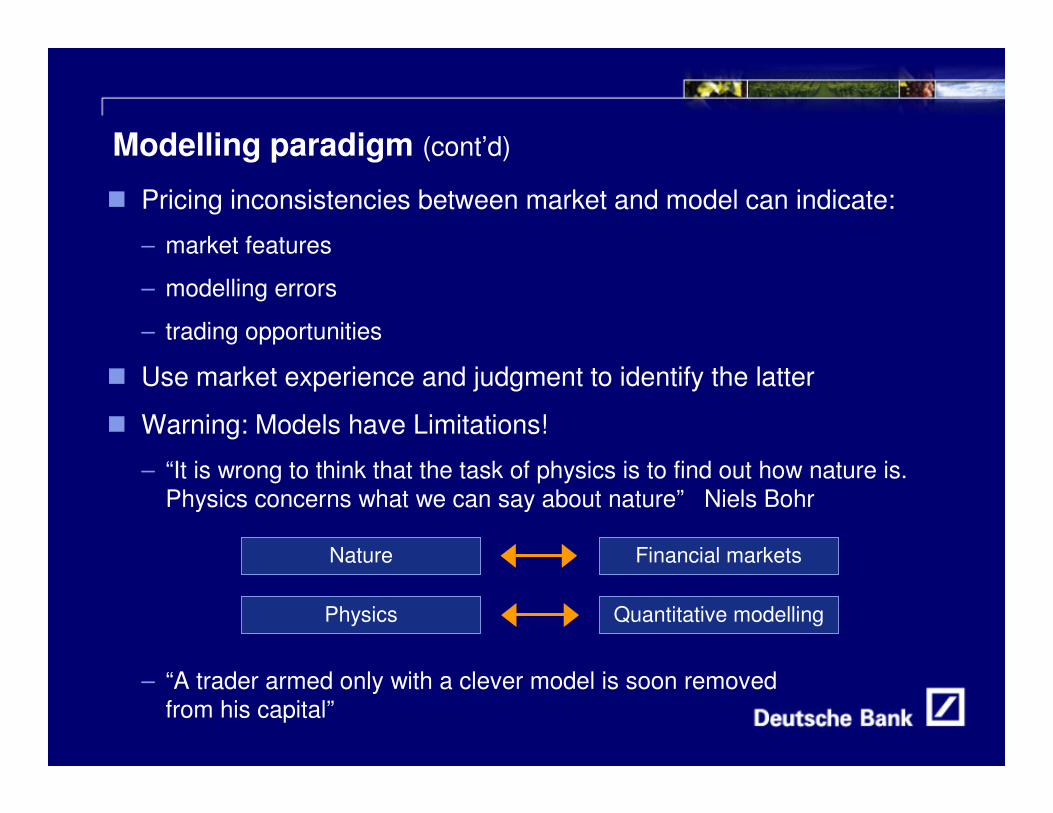
Modelling paradigm (cont’d)
� Pricing inconsistencies between market and model can indicate:
– market features
– modelling errors
– trading opportunities
� Use market experience and judgment to identify the latter
� Warning: Models have Limitations!
– “It is wrong to think that the task of physics is to find out how nature is. Physics concerns what we can say about nature” Niels Bohr
– “A trader armed only with a clever model is soon removed from his capital”
Nature Financial markets
Physics Quantitative modelling
5
Modelling paradigm (cont’d)
� Significant advances in quantitative financial modelling over past ten years. Need judgment to harness these advances
� Tukey: judgment based on
– mathematical knowledge of the particular techniques
– experience of the particular field of subject matter
– experience of how these techniques have worked out in practice
6
Forward volatility surfaces
� Translate universe of option prices into how each point on yieldcurve (e.g. each Euribor future) oscillates over time
� More precisely: strip swaptions, caps and other option products into a forward volatility surface, σ (t,T)
� For fixed T, σ (t,T) represents the volatility of a particular Eurodollar (or Euribor) contract over its life. These “forward volatilities” are observable quantities about which can make subjective judgments

7
Forward volatility surfaces (cont’d)
� Framework adopts multifactor BGM Model
df(t, T) = a(t,T) dt + σσσσ(t, T) ΣΣΣΣ ρρρρi (t, T) dWi (t)
– f (t , T) 3m-forward rate from T at time t
– Drift a(t, T) determined from volatility σ(t, T)
n
i = 1
8
Forward volatility surfaces (cont’d)
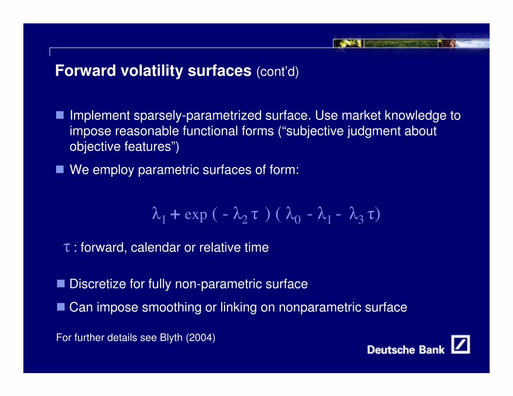
� Implement sparsely-parametrized surface. Use market knowledge to impose reasonable functional forms (“subjective judgment about objective features”)
� We employ parametric surfaces of form:
� Discretize for fully non-parametric surface
� Can impose smoothing or linking on nonparametric surface
For further details see Blyth (2004)
�1 + exp ( - �2 � ) ( �0 - �1 - �3 �)
� : forward, calendar or relative time
9
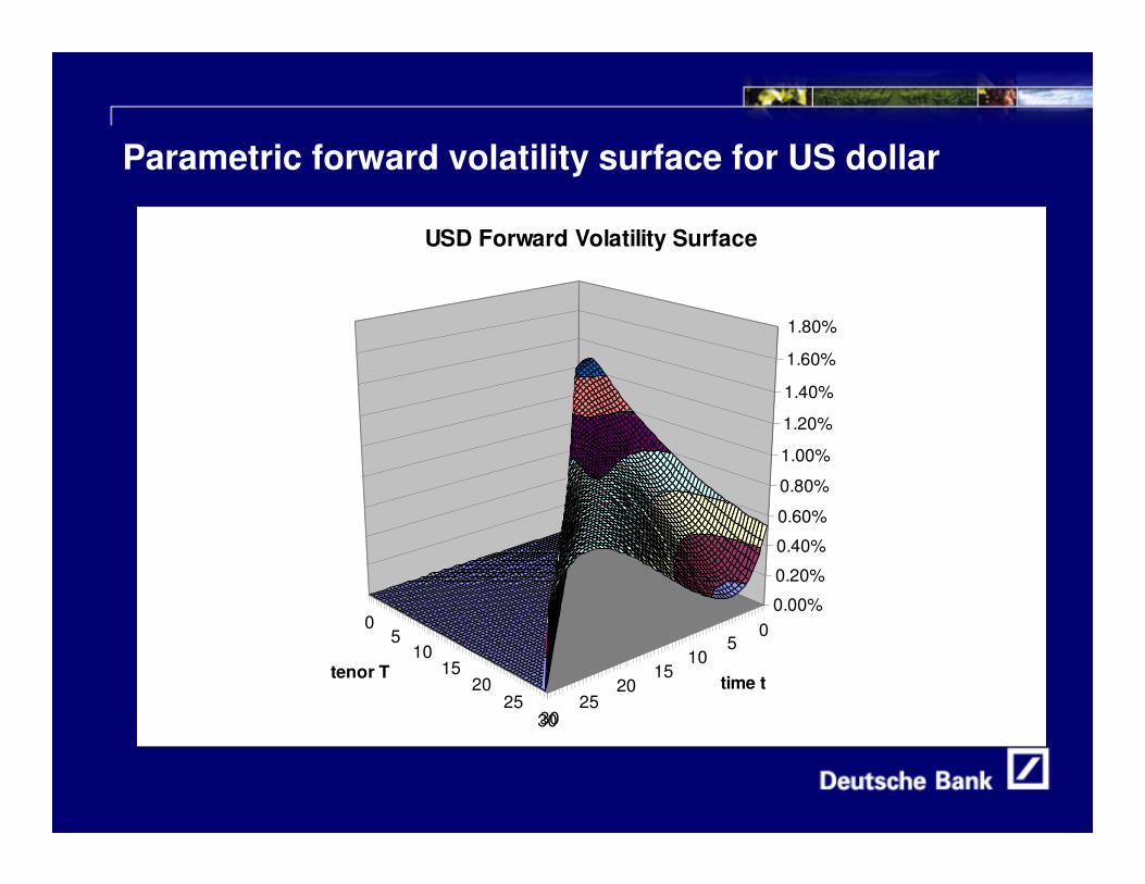
Parametric forward volatility surface for US dollar
05
1015
2025
30
05
1015
2025
30
0.00%
0.20%
0.40%
0.60%
0.80%
1.00%
1.20%
1.40%
1.60%
1.80%
time ttenor T
USD Forward Volatility Surface
10
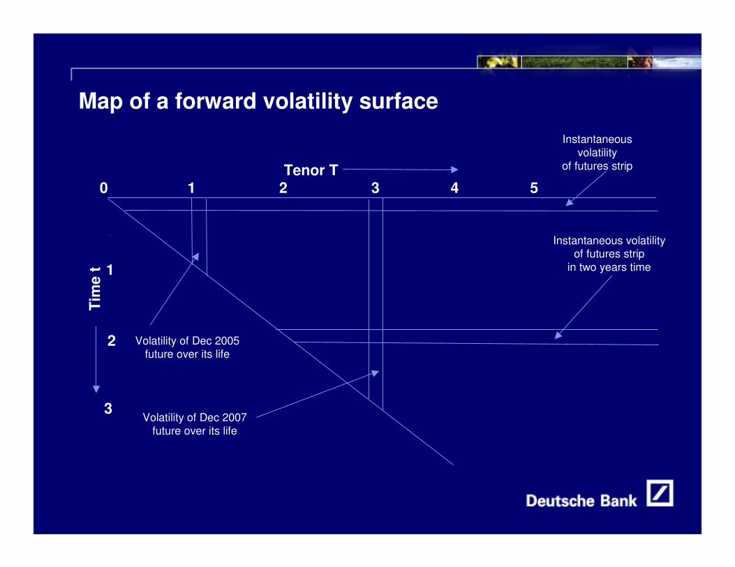
Map of a forward volatility surface
0 1 2 3 4 5Tenor T
1
2
3
Instantaneous volatility
of futures strip
Instantaneous volatilityof futures strip
in two years time
Volatility of Dec 2005future over its life
Volatility of Dec 2007 future over its life
Tim
e t
11
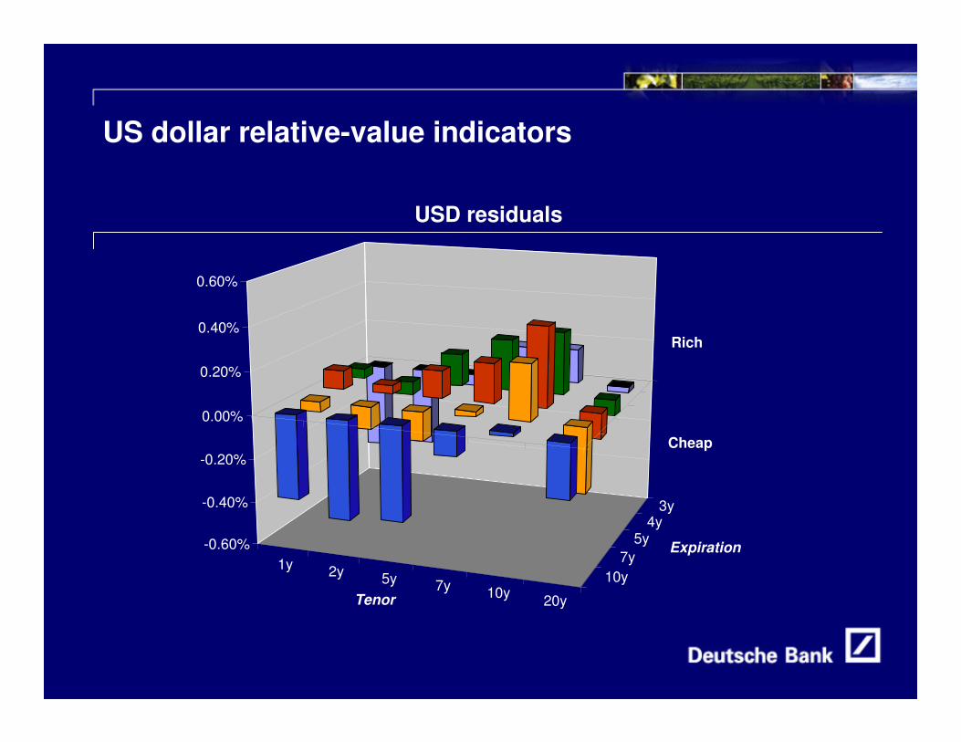
US dollar relative-value indicators
1y 2y 5y 7y 10y 20y
3y4y
5y7y
10y
-0.60%
-0.40%
-0.20%
0.00%
0.20%
0.40%
0.60%
Tenor
Expiration
Rich
Cheap
USD residuals
12
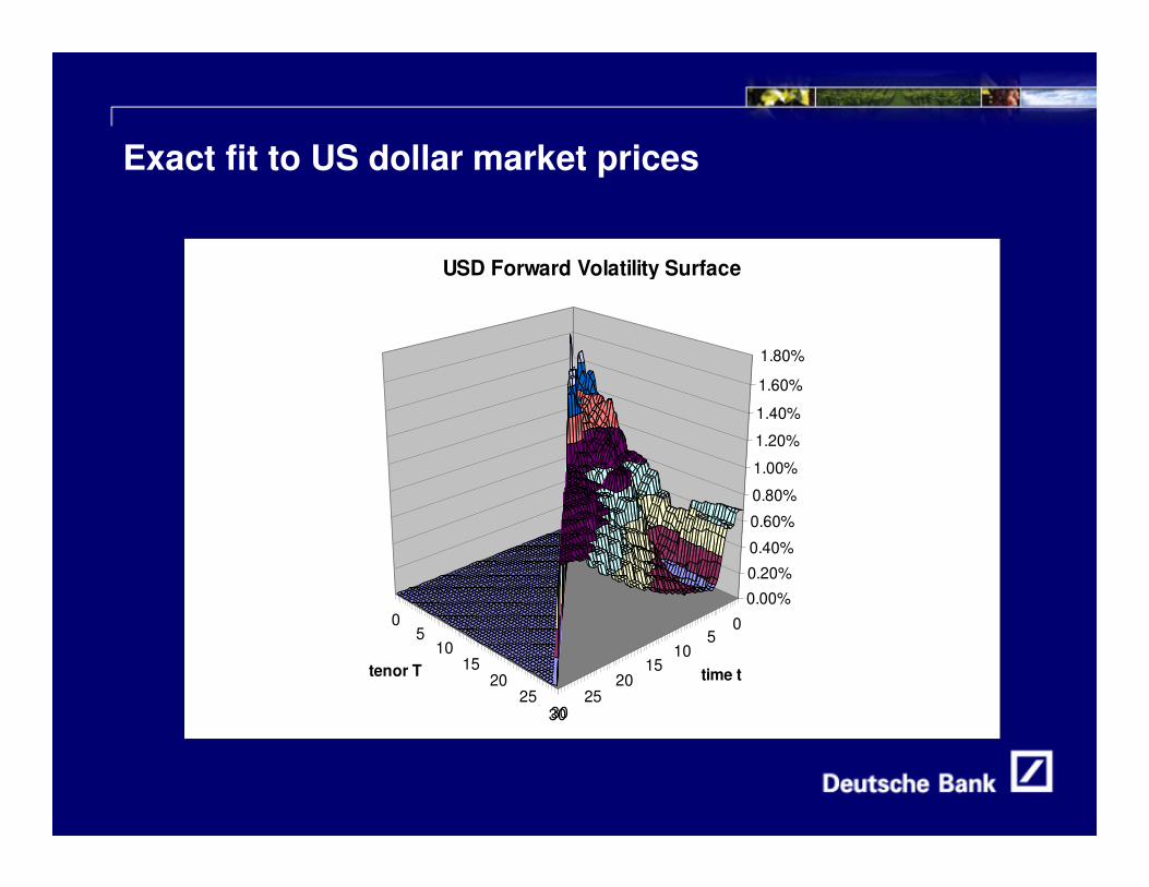
Exact fit to US dollar market prices
05
1015
2025
30
05
1015
2025
30
0.00%
0.20%
0.40%
0.60%
0.80%
1.00%
1.20%
1.40%
1.60%
1.80%
time ttenor T
USD Forward Volatility Surface
13
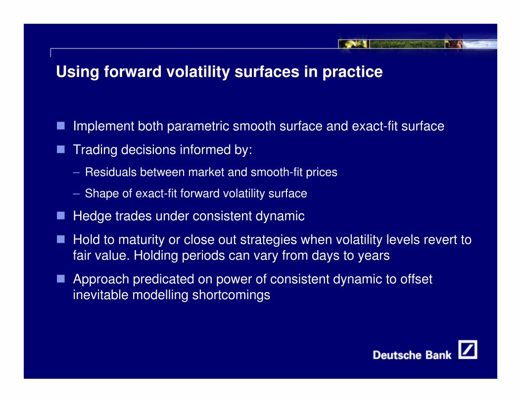
Using forward volatility surfaces in practice
� Implement both parametric smooth surface and exact-fit surface
� Trading decisions informed by:
– Residuals between market and smooth-fit prices
– Shape of exact-fit forward volatility surface
� Hedge trades under consistent dynamic
� Hold to maturity or close out strategies when volatility levels revert to fair value. Holding periods can vary from days to years
� Approach predicated on power of consistent dynamic to offset inevitable modelling shortcomings
14
Further examples 1. Hedge 10yr CMS liabilities with 5yr-tailed swaptions
� 10yr-tailed swaptions are rich due to hedging of 10yr CMS product
� Portfolio of 5yr-tail options with spectrum of expirations captures similar volatility, but at cheaper levels
– 10yr-5yr and 15yr-5yr payers are better value than 10yr-10yr payer
15
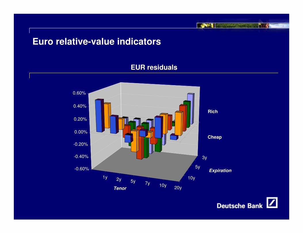
Euro relative-value indicators
EUR residuals
-0.60%
-0.40%
-0.20%
0.00%
0.20%
0.40%
0.60%
1y 2y 5y 7y 10y 20yTenor
3y
5y
10y
Expiration
Cheap
Rich

16
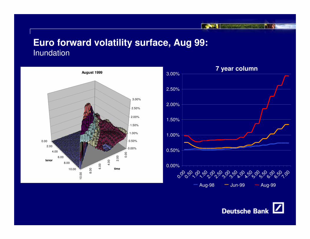
2. Caps versus swaptions, 1998-9
� Unwind of proprietary desks’ short positions in caps versus longpositions in swaptions widened volatility spread between products
� In forward volatility space, this resulted in large spikes in forward volatility of the front contracts
� Volatility dynamic implied by these prices absurd

17
Euro forward volatility surface, Aug 98-June 99:The approach of the storm
0.00
2.00
4.00
6.00
8.00
10.0
0
0.00
2.00
4.00
6.00
8.00
10.00
0.00%
0.50%
1.00%
1.50%
2.00%
2.50%
3.00%
time
tenor
June 1999
0.00
2.00
4.00
6.00
8.00
10.0
0
0.00
2.00
4.00
6.00
8.00
10.00
0.00%
0.50%
1.00%
1.50%
2.00%
2.50%
3.00%
time
tenor
August 1998
18
Euro forward volatility surface, Aug 99:Inundation
0.00
2.00
4.00
6.00
8.00
10.0
0
0.00
2.00
4.00
6.00
8.00
10.00
0.00%
0.50%
1.00%
1.50%
2.00%
2.50%
3.00%
time
tenor
August 1999
0.00%
0.50%
1.00%
1.50%
2.00%
2.50%
3.00%
0.00
0.50
1.00
1.50
2.00
2.50
3.00
3.50
4.00
4.50
5.00
5.50
6.00
6.50
7.00
Aug-98 Jun-99 Aug-99
7 year column
19
3. Euro swaption relative value: comparing indicators
� Consistent modelling framework can identify better trading strategies to simpler historical implied analysis - although often indicators concur.
� Consider performance of relative-value trades in euro swaption market.

20
Euro swaption relative value (cont’d)
Relative Value Indicators
-4%
-2%
0%
2%
4%
6%
8%
10%
12%
Jan-02 Jul-02 Jan-03 Jul-03 Jan-04 Jul-04
Perc
enta
ge R
ich/
Che
ap
Buy 2y5ySell 2y20y
Buy 1y5ySell 1y20y

21
Euro swaption relative value (cont’d)
Ratio of Implied Normalised Volatilities
1.05
1.10
1.15
1.20
1.25
1.30
1.35
1.40
Jan-02 Jul-02 Jan-03 Jul-03 Jan-04 Jul-04
2y-5y/2y-20y
1y-5y/1y-10y
22
Additional dimensions
� Skew Modelling: demand consistency between pricing of skew and
dynamics of implied volatility under market movements
� Term Structure of Skew: skew structure for short-term rates coupled
with specified dynamics may not be consistent with certain skew
structure for longer-dated rates
� Stochastic Volatility: demand consistency between stochastic
volatility overlays used to price option smile and prices of compound
options
Practical Relative-Value Volatility Trading
Stephen Blyth,
Managing Director, Head of European Arbitrage Trading
21 January 2005