voltage stability analysis of the nigerian power …

* Corresponding author, tel: +234 803 667 5952

VOLTAGE STABILITY ANALYSIS OF THE NIGERIAN POWER SYSTEM

USING ANNEALING OPTIMIZATION TECHNIQUE

M. J. Mbunwe 1,* and A. O. Ekwue2 1, DEPARTMENT OF ELECTRICAL ENGINEERING, UNIVERSITY OF NIGERIA, NSUKKA, ENUGU STATE, NIGERIA

2, JACOBS ENGINEERING INC/ BRUNEL UNIVERSITY LONDON, UNITED KINGDOM

E-mail addresses: 1 [email protected], 2 [email protected]

ABSTRACT

The paper addresses the means of overcoming the challenge posed by voltage collapse to the

stability of the Nigerian electric power system. The technique applied is based on time identification

algorithm elaborating, at a given grid bus, the local phasor measurements at fast sampling rate.

Elements such as adjustable shunt compensation devices, generator reactive generation,

transformer tap settings are optimally adjusted at each operating point to reach the objective of

minimizing the voltage stability index at each individual bus as well as minimizing the global

voltage stability indicator. The control elements setting were optimized and the maximum possible

MVA voltage stable loading has been achieved and a best voltage profile was obtained. Results of

tests conducted on a 6-bus IEEE system and a typical 28-bus Nigerian power distribution network

are presented and discussed.

Keywords: Special protection systems, voltage stability analysis, voltage stability limit, voltage collapse

mechanism, system security

1. INTRODUCTION

As regards the record available from the recent

deregulation of the generation and distribution

segment of many electric power systems in the

world including Nigeria’s, it has become evidently

necessary to investigate the best operating

conditions under which the transmission system is

expected to perform with respect to the high level of

transactions expected to always take place.

Moreover, it is quite devastating that voltage

collapse has remained one of the unresolved riddles

that are currently plaguing the power system

operation and performance under the recent

electricity regime leading to blackout or abnormally

low voltages in a significant part of the power

system. Special protection Schemes (SPS) have

been widely used to increase the transfer capability

of the network by assisting system operators in

administering fast corrective actions. The cause of

this instability can be categorized into technical and

non-technical. The technical causes may be due to

tripping of lines on account of faulty equipment or

increase in load than the available supply [1].

The power system ability to maintain constantly

acceptable bus voltage at each node under normal

operating conditions, after load increase, following

system configuration changes or when the system is

being subjected to a disturbance is a very important

characteristic of the system. The non-optimized

control of VAR resources may lead to progressive

and uncontrollable drop in voltage resulting in an

eventual wide spread voltage collapse.

The phenomenon of voltage instability is attributed

to the power system operation at its maximum

transmissible power limit, shortage of reactive power

resources and inadequacy of reactive power

compensation tools. A non-optimized setting of the

level or control of the reactive resources plays an

effective role to expedite the voltage instability and

to speed up reaching the maximum loading limit.

The main factors contributing to the voltage collapse

are the generators reactive power limit, load

characteristics, voltage control limits, reactive

Nigerian Journal of Technology (NIJOTECH)

Vol. 39, No. 2, April 2020, pp. 562- 571

Copyright© Faculty of Engineering, University of Nigeria, Nsukka, Print ISSN: 0331-8443, Electronic ISSN: 2467-8821

www.nijotech.com

http://dx.doi.org/10.4314/njt.v39i2.27

http://www.nijotech.com/

http://dx.doi.org/10.4314/njt.v39i2.27

VOLTAGE STABILITY ANALYSIS OF THE NIGERIAN POWER SYSTEM USING ANNEALING OPTIMIZATION TECHNIQUE, M. J. Mbunwe & A. O. Ekwue

Nigerian Journal of Technology, Vol. 39, No. 2, April 2020 563

compensation devices characteristics and their

reactions.

Voltage stability estimation techniques based on

load flow Jacobian analysis such as, singular value

decomposition, eigen value calculations, sensitivity

factories, and modal analysis are time consuming for

a large power system [2- 6]. Several indices based

methods such as Voltage Instability Proximity Index

(VIPI) and Voltage Collapse Proximity Indicator

(VCPI) are used to evaluate voltage instability.

These are based on multiple load flow solutions and

give only global picture [7, 8]. The transmission

proximity index that specifies the weakest

transmission part of the system based on voltage

phasor approach necessitate the scanning of the

whole power system structure for several times

which is the time consuming approach [9].

The strong tie of the voltage stability problem with

the reactive power resources and flow in the system

raise the interest in optimizing the rescheduling of

the VAR control tools [10]. An optimum VAR picture

would maintain a good voltage profile and extend

the maximum loading capability of the power

network [11]. Many researchers reported on several

approaches for optimal reactive power, dc-based

techniques and features of accurate voltage-based

contingency selection algorithm [12], in literature.

Methods such as linear programming and nonlinear

programming algorithms were applied. They are

complex, time consuming and require considerable

amount of memory [13 -19].

The non-incremental quadratic programming model

used for optimal reactive power control, though the

technique is relatively accurate and shows a

satisfactory convergence characteristic but as the

system gets bigger the number of variables to be

evaluated would rise sharply [20].

This paper proposes an optimized fast voltage

stability indicator dedicated for evaluation and

monitoring. The optimized index gives information

covering the whole power system and evaluated at

each individual bus, this is calculated at every

operating point. The used indicator is simple to

derive and fast to calculate. In order to enhance the

voltage stability profile throughout the whole power

network, simulated annealing (SA) optimization

technique [21, 22] is applied to control the power

elements of major influence on the voltage stability

profile. Elements such as generator reactive

generation, adjustable shunt compensation devices,

transformer tap settings are optimally adjusted at

each operating point to reach the objective of

increasing the distance from an unstable system

state and therefore to increase the maximum

possible system safe loading. The objective is

achieved through minimizing the L-index values at

every bus of the system and consequently the global

power system L-index.

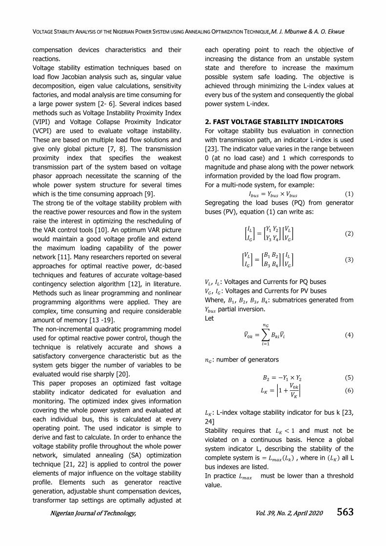
2. FAST VOLTAGE STABILITY INDICATORS

For voltage stability bus evaluation in connection

with transmission path, an indicator L-index is used

[23]. The indicator value varies in the range between

0 (at no load case) and 1 which corresponds to

magnitude and phase along with the power network

information provided by the load flow program.

For a multi-node system, for example:

𝐼𝑏𝑢𝑠 = 𝑌𝑏𝑢𝑠 × 𝑉𝑏𝑢𝑠 (1)

Segregating the load buses (PQ) from generator

buses (PV), equation (1) can write as:

[𝐼𝐿

𝐼𝐺

] = [𝑌1

𝑌3

𝑌2

𝑌4

] [𝑉𝐿

𝑉𝐺

] (2)

[𝑉𝐿

𝐼𝐺

] = [𝐵1

𝐵3

𝐵2

𝐵4

] [𝐼𝐿

𝑉𝐺

] (3)

𝑉𝐿, 𝐼𝐿: Voltages and Currents for PQ buses

𝑉𝐺, 𝐼𝐺: Voltages and Currents for PV buses

Where, 𝐵1, 𝐵2, 𝐵3, 𝐵4: submatrices generated from

𝑌𝑏𝑢𝑠 partial inversion.

Let

�̅�0𝑘 = ∑ 𝐵𝑘𝑖�̅�𝑖

𝑛𝐺

𝑖=1

(4)

𝑛𝐺: number of generators

𝐵2 = −𝑌1 × 𝑌2 (5)

𝐿𝐾 = |1 +𝑉0𝑘

𝑉𝐾

| (6)

𝐿𝐾: L-index voltage stability indicator for bus k [23,

24]

Stability requires that 𝐿𝐾 < 1 and must not be

violated on a continuous basis. Hence a global

system indicator L, describing the stability of the

complete system is = 𝐿𝑚𝑎𝑥(𝐿𝑘) , where in (𝐿𝐾) all L

bus indexes are listed.

In practice 𝐿𝑚𝑎𝑥 must be lower than a threshold

value.



The predetermined threshold value is specified at

the planning stage depending on the system

configuration and on the utility policy regarding the

quality of service and the level of system decided

allowable margin. In practice, the calculation of the

complex vector kV0 never uses the inversion of 1Y.

[−𝑌1]𝑉0𝑘 = [𝑌2]𝑉𝐺 (7)

Sparse factorization vector methods have been used

to solve the linear system in equation (7) and make

from L-index a potential candidate for real-time

performance [23, 24]

3. SIMULATED TECHNIQUES

3.1 Brief Introduction

Simulated annealing (SA) is an optimization

technique that simulates the physical annealing

process in the field that combine optimization.

Annealing is the physical process of heating up a

solid until it melts, followed by slow cooling it down

by decreasing the temperature of the environment

in steps. At each step, the temperature is maintained

constant for a period of time sufficient for the solid

to reach thermal equilibrium.

The research work [22] proposed a Monte Carlo

method to simulate the process of reaching thermal

equilibrium at a fixed value of the temperature T. In

this method, a randomly generated perturbation of

the current configuration of the solid is applied so

that a trial configuration is obtained. This trial

configuration is accepted and becomes the current

configuration if it satisfies an acceptance criterion.

The process continues until the thermal equilibrium

is achieved after a large number of perturbations. By

gradually decreasing the temperature T and

repeating [2, 22] simulation, new lower energy

levels become achievable. As T approaches zero

least energy configurations will have a positive

probability of occurring.

3.2 Simulated Annealing Algorithm

At first, the analogy between a physical annealing

process and a combinatorial optimization problem is

based on the following [21]:

solutions in an optimization problem are

equivalent to configurations of a physical

system.

the cost of a solution is equivalent to the

energy of a configuration.

In addition, a control parameter pC is introduced to

play the role of the temperature T.

The basic elements of SA are defined as follows:-

Current, trial, and best solutions:

𝑥𝑐𝑢𝑟𝑟𝑒𝑛𝑡 , 𝑥𝑡𝑟𝑖𝑎𝑙 , and 𝑥𝑏𝑒𝑠𝑡: these solutions are

sets of the optimized parameter values at

any iteration.

Acceptance criterion: at any iteration, the

trial solution can be accepted as the current

solution if it meets one of the following

criteria:

(a) 𝑱(𝒙𝒕𝒓𝒊𝒂𝒍) < 𝑱(𝒙𝒄𝒖𝒓𝒓𝒆𝒏𝒕); (b) 𝑱(𝒙𝒕𝒓𝒊𝒂𝒍) > 𝑱(𝒙𝒄𝒖𝒓𝒓𝒆𝒏𝒕) and

𝑒𝑥𝑝(− (𝐽(𝑥𝑡𝑟𝑖𝑎𝑙) − 𝐽(𝑥𝑐𝑢𝑟𝑟𝑒𝑛𝑡)) 𝐶𝑝⁄ ) ≥ 𝑟𝑎𝑛𝑑(0, 1).

Where, 𝑟𝑎𝑛𝑑(0, 1) is a random number with

domain (0, 1) and 𝐽(𝑥𝑡𝑟𝑖𝑎𝑙) and 𝐽(𝑥𝑐𝑢𝑟𝑟𝑒𝑛𝑡) are the

objective function values associated with 𝑥𝑡𝑟𝑖𝑎𝑙 and

𝑥𝑐𝑢𝑟𝑟𝑒𝑛𝑡 respectively. Criterion (b) indicates that the

trial solution is not necessarily rejected if its

objective function is not as good as that of the

current solution with hoping that a much better

solution becomes reachable.

Acceptance ratio: at a given value of 𝐶𝑝,

an 𝑛1 trial solution can be randomly

generated. Based on the acceptance

criterion, an 𝑛2 of these solutions can be

accepted. The acceptance ratio is defined

as𝑛2

𝑛1⁄ .

Cooling schedule: it specifies a set of

parameters that governs the convergence of

the algorithm. This set includes an initial

value of control parameter 𝐶0𝑝, a decrement

function for decreasing the value of 𝐶𝑝, and

a finite number of iterations or transitions at

each value of 𝐶𝑝, that is, the length of each

homogeneous Markov chain. The initial

value of 𝐶𝑝 should be large enough to allow

virtually all transitions to be accepted.

However, this can be achieved by starting off at a

small value of 𝐶0𝑝 and multiplying it with a constant

larger than 1, that is 𝐶0𝑝 = 𝛼𝐶0𝑝. This process

continues until the acceptance ratio is close to 1.

This is equivalent to heating up process in physical

systems.

The decrement function for decreasing the value of

𝐶𝑝 is given by 𝐶𝑝 = 𝜇𝐶𝑝

Where, 𝜇 is a constant smaller than but close to 1.

Typical values lie between 0.8 and 0.99 [21].



Equilibrium condition: it occurs when the

current solution does not change for a

certain number of iterations at a given value

of 𝐶𝑝. It can be achieved by generating

many transitions at that value of 𝐶𝑝.

Stopping Criteria: these are the

conditions under which the search process

will terminate.

In this study, the search will terminate if one of the

following criteria is satisfied:

(a) the number of Markov chains since the last

change of the best solution is greater than a

prespecified number; or,

(b) the number of Markov chains reaches the

maximum allowable number.

The SA algorithm can be described in steps as

follows:

Step 1: Set the initial value of 𝐶0𝑝 and randomly

generate an initial solution 𝑥𝑖𝑛𝑖𝑡𝑖𝑎𝑙 and calculate its

objective function. Set this solution as the current

solution as well as the best solution, i.e. 𝑥𝑖𝑛𝑖𝑡𝑖𝑎𝑙 =

𝑥𝑐𝑢𝑟𝑟𝑒𝑛𝑡 = 𝑥𝑏𝑒𝑠𝑡.

Step 2: Randomly generate an 1n of trial solutions

about the current solution.

Step 3: Check the acceptance criterion of these trial

solutions and calculate the acceptance ratio. If

acceptance ratio is close to 1 go to step 4; else set

𝐶0𝑝 = 𝛼𝐶0𝑝, 𝛼 > 1, and go back to step 2.

Step 4: Set the chain counter 𝐾𝑐ℎ = 0.

Step 5: Generate a trial solution trialx. If 𝑥𝑡𝑟𝑖𝑎𝑙

satisfies the acceptance criterion set

𝑥𝑐𝑢𝑟𝑟𝑒𝑛𝑡 = 𝑥𝑡𝑟𝑖𝑎𝑙, 𝐽(𝑥𝑐𝑢𝑟𝑟𝑒𝑛𝑡) = 𝐽(𝑥𝑡𝑟𝑖𝑎𝑙), and go to step

6; else go to step 6.

Step 6: Check the equilibrium condition. If it is

satisfied go to step 7; else go to step 5.

Step 7: Check the stopping criteria. If one of them

is satisfied then stop; else set 𝐾𝑐ℎ = 𝐾𝑐ℎ + 1 and

𝐶𝑝 = 𝜇𝐶𝑝, 𝜇 < 1, and go back to Step 5.

4. TEST RESULTS AND DISCUSSION

The demonstrated is applied on IEEE 6-bus test

system [25] which has two voltage sources and four

load buses. Bus-1 is the swing bus, bus 2 is PV bus

and buses 3-6 are PQ load buses. It is also tested on

a typical practical Nigerian 28-bus Network (Nsukka

11kV Campus Feeder Network).

4.1 Case 1: 6 Bus Network

The single –line diagram of the 6-bus IEEE network

is shown in Figure 1 with line data and bus data are

given in Tables 1 and 2 respectively.

The voltage stability index is evaluated at every

operating point and for every bus in the system

along the system overall index 𝐿𝑚𝑎𝑥. The simulated

annealing optimization is activated of every

operating in order to adjust the available VAR control

tools for the objective of minimizing the value of L-

index at every bus in the system and consequently

the system overall voltage stability indicator 𝐿𝑚𝑎𝑥.

Hence, the optimization problem can be written as

𝑀𝑖𝑛𝑖𝑚𝑖𝑧𝑒 (𝑚𝑎𝑥(𝐿𝑘; 𝑘 = 1, 2, … , 𝑛)) (8)

𝑛: number of buses

The problem constraints are the control variable

bounds as given in Table 3.

The optimal values of control variables are given in

Table 3 which also shows the load flow solution with

the initial settings and the proposed optimal settings

of the control variables. It is clear that the voltage

profile is greatly improved and the real power loss is

reduced by 11.32%.

Table 4 shows a comparative list of results using

both voltage stability evaluation of L-index with and

without optimization.

It can be seen that the values of L-index at load

buses are reduced; therefore, the voltage stability of

the system is enhanced and improved.

The test was carried out for a different load level

starting from 40% of the base load with a step

increase of all loads in the system till voltage

collapse.

The voltages of load buses versus load factor

without and with optimization are as shown in Figure

3.

In addition, L-index values at load buses versus load

factor are as shown in Figure 4.

It is clear that the application of the SA algorithm

has significantly reduced the values of L-index all

over the system. Consequently, the voltage stability

distance from collapse has increased. The gain in

power system MVA loading was found to be 23%.

The above positive results demonstrate the potential

of the proposed approach to improve and enhance

the system voltage stability.



4.2 Case 2: Typical 28 Bus Nigerian Networks

The line diagram of a typical 28-bus Nigerian

network (Nsukka 11kV Campus Feeder) [26] is as

shown in Figure 5 with network bus details and line

indications presented in Table 5 and 6 respectively.

The objective function convergence rate is shown in

Figure 2 and this shows the fast convergence of the

proposed technique.

Fig. 1: Line Diagram of IEEE 6-Bus System

Table 1: Line Data on 100 MVA base

Line number From To R (pu) X (pu)

1 1 6 0.1230 0.518

2 1 4 0.0800 0.370

3 2 3 0.0723 1.050

4 2 5 0.2820 0.064

5 3 4 0.0000 0.133

6 4 6 0.0970 0.407

7 6 5 0.0000 0.300

Fig. 2: Objective function convergence

Table 2: IEEE 6-Bus Data on 100 MVA base

Bus number Voltage (pu)

Pg (pu) Qg (pu) PL (pu) QL (pu) V Q

1 1.0500 0.0000 0.9662 0.3792 0.0000 0.0000

2 1.1000 -06.1494 0.5000 0.3499 0.0000 0.0000 3 0.8563 -13.8236 ---- ---- 0.5500 0.1300

4 0.9528 -09.9245 ---- ---- 0.0000 0.0000 5 0.8992 -13.4205 ---- ---- 0.3000 0.1800

6 0.9338 -12.6485 ---- ---- 0.5000 0.0500

Table 3: Load flow results without and with optimization

Variable Limits

Without Optimization With Optimization Low High

Control Variables Transformer Taps T4;

T6

0.90

0.90

1.10

1.10

1.025

1.100

0.958

0.984 Generator voltage (pu) V1;

V2

1.00

1.10

1.10

1.15

1.050

1.100

1.092

1.150

Dependent Variables Generator MVAR Qg1;

Qg2

-20.0

-20.0

100.0

100.0

38.11

34.80

35.82

19.35

Voltages at load Buses (pu) V3; V4;

V5; V6

0.90

0.90 0.90

0.90

1.00

1.00 1.00

1.00

0.855

0.953 0.901

0.933

1.001

1.001 1.000

0.984 System Losses (MW) ---- ---- 11.61 8.880



Table 4: Behavior of L-index with and without optimization

Bus number L-index without

optimization

L-index with

optimization

3 0.288 0.234 4 0.211 0.178

5 0.278 0.234 6 0.258 0.218

(a) Without optimization

(b) With Optimization

Fig. 3: Load buses voltages

Without optimization With optimization

Fig. 4: Load buses Lindex values (a) Without

optimization (b) With optimization

The optimal values of control variables are given in

Table 3 as well as Table 7, which also shows the load

flow solution with the initial settings and the

proposed optimal settings of the control variables. It

is clear that the voltage profile is greatly improved

and the real power loss is reduced by 11.32% also.

Table 4 as well as Table 8 also shows a comparative

list of results using both voltage stability evaluation

of L-index with and without optimization from the

existing and the proposed.

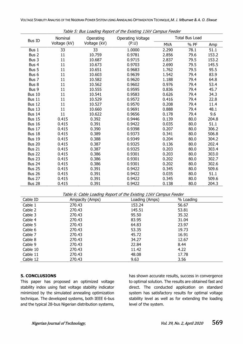
The Table 5 shows the bus loading report of the

existing 11kV Campus Feeder.

The Table 6 shows the Cable Loading Report of the

Existing 11kV Campus Feeder.

Similarly, the voltage stability index was also

evaluated at every operating point and for every bus

in the system along the system overall index 𝐿𝑚𝑎𝑥.

The simulated annealing optimization was activated

of every operating in order to adjust the available

VAR control tools for the objective of minimizing the

value of L-index at every bus in the system and

consequently the system overall voltage stability

indicator 𝐿𝑚𝑎𝑥.



Fig. 5: Nsukka 11kV Campus Network System



Table 5: Bus Loading Report of the Existing 11kV Campus Feeder

Bus ID Nominal

Voltage (kV)

Operating

Voltage (kV)

Operating Voltage

(P.U)

Total Bus Load

MVA % PF Amp

Bus 1 33 33 1.0000 2.290 78.1 51.1

Bus 2 11 10.759 0.9781 2.856 79.6 153.2

Bus 3 11 10.687 0.9715 2.837 79.5 153.2 Bus 4 11 10.673 0.9703 2.690 79.5 145.5

Bus 5 11 10.651 0.9683 1.762 79.5 95.5 Bus 6 11 10.603 0.9639 1.542 79.4 83.9

Bus 7 11 10.582 0.9620 1.188 79.4 64.8

Bus 8 11 10.562 0.9602 0.976 79.4 53.4 Bus 9 11 10.555 0.9595 0.836 79.4 45.7

Bus 10 11 10.541 0.9583 0.626 79.4 34.3 Bus 11 11 10.529 0.9572 0.416 79.4 22.8

Bus 12 11 10.527 0.9570 0.208 79.4 11.4

Bus 13 11 10.660 0.9691 0.888 79.4 48.1 Bus 14 11 10.622 0.9656 0.178 79.4 9.6

Bus 15 0.415 0.392 0.9446 0.139 80.0 204.8 Bus 16 0.415 0.391 0.9422 0.035 80.0 51.1

Bus 17 0.415 0.390 0.9398 0.207 80.0 306.2 Bus 18 0.415 0.389 0.9373 0.341 80.0 506.8

Bus 19 0.415 0.388 0.9349 0.204 80.0 304.2

Bus 20 0.415 0.387 0.9325 0.136 80.0 202.4

Bus 21 0.415 0.387 0.9325 0.203 80.0 303.4

Bus 22 0.415 0.386 0.9301 0.203 80.0 303.0 Bus 23 0.415 0.386 0.9301 0.202 80.0 302.7

Bus 24 0.415 0.386 0.9301 0.202 80.0 302.6 Bus 25 0.415 0.391 0.9422 0.345 80.0 509.6

Bus 26 0.415 0.391 0.9422 0.035 80.0 51.1 Bus 27 0.415 0.391 0.9422 0.345 80.0 509.6

Bus 28 0.415 0.391 0.9422 0.138 80.0 204.3

Table 6: Cable Loading Report of the Existing 11kV Campus Feeder Cable ID Ampacity (Amps) Loading (Amps) % Loading

Cable 1 270.43 153.24 56.67 Cable 2 270.43 145.51 53.81

Cable 3 270.43 95.50 35.32 Cable 4 270.43 83.95 31.04

Cable 5 270.43 64.83 23.97

Cable 6 270.43 53.35 19.73 Cable 7 270.43 45.72 16.91

Cable 8 270.43 34.27 12.67 Cable 9 270.43 22.84 8.44

Cable 10 270.43 11.42 4.22

Cable 11 270.43 48.08 17.78 Cable 12 270.43 9.63 3.56

5. CONCLUSIONS

This paper has proposed an optimized voltage

stability index using fast voltage stability indicator

minimized by the simulated annealing optimization

technique. The developed systems, both IEEE 6-bus

and the typical 28-bus Nigerian distribution systems,

has shown accurate results, success in convergence

to optimal solution. The results are obtained fast and

direct. The conducted application on standard

system has satisfactory results for optimal voltage

stability level as well as for extending the loading

level of the system.



Table 7: Bus Loading Report of the Proposed 11kV Campus Feeder Bus ID Nominal

Voltage (kV) Operating Voltage (kV)

Operating Voltage (P.U)

Total Bus Load

MVA % PF Amp

Bus 1 33 33 1.000 2.422 99.5 42.4

Bus 2 11 10.952 0.9956 2.411 99.7 127.1 Bus 3 11 10.895 0.9905 2.399 99.8 127.1

Bus 4 11 10.884 0.9894 2.276 99.7 120.7 Bus 5 11 10.866 0.9878 1.492 99.7 79.3

Bus 6 11 10.828 0.9844 1.308 99.7 69.7

Bus 7 11 10.811 0.9828 1.008 99.7 53.9 Bus 8 11 10.795 0.9814 0.829 99.7 44.3

Bus 9 11 10.790 0.9809 0.710 99.7 38.0 Bus 10 11 10.779 0.9799 0.532 99.7 28.5

Bus 11 11 10.769 0.9790 0.354 99.7 19.0

Bus 12 11 10.768 0.9789 0.177 99.7 9.5 Bus 13 11 10.875 0.9886 0.750 99.8 39.8

Bus 14 11 10.874 0.9885 0.151 99.9 8.0 Bus 15 0.415 0.405 0.9759 0.149 80.0 211.9

Bus 16 0.415 0.406 0.9783 0.041 73.2 58.0

Bus 17 0.415 0.404 0.9734 0.222 80.0 316.8 Bus 18 0.415 0.402 0.9687 0.366 80.0 524.7

Bus 19 0.415 0.402 0.9687 0.219 80.0 315.2 Bus 20 0.415 0.401 0.9663 0.146 80.0 209.9

Bus 21 0.415 0.401 0.9663 0.218 80.0 314.6 Bus 22 0.415 0.401 0.9663 0.218 80.0 314.2

Bus 23 0.415 0.400 0.9639 0.218 80.0 313.9

Bus 24 0.415 0.400 0.9639 0.218 80.0 313.9 Bus 25 0.415 0.404 0.9734 0.369 80.0 527.0

Bus 26 0.415 0.406 0.9783 0.041 73.2 58.0 Bus 27 0.415 0.404 0.9734 0.369 80.0 527.0

Bus 28 0.415 0.404 0.9734 0.148 80.0 211.4

Table 8: Cable Loading Report of the Proposed 11kV Campus Feeder

Cable ID Ampacity (Amps)

Loading (Amps)

% Loading

Cable 1 270.43 127.11 47.00

Cable 2 270.43 120.72 44.64 Cable 3 270.43 79.29 29.32

Cable 4 270.43 69.72 25.78 Cable 5 270.43 53.85 19.91

Cable 6 270.43 44.33 16.39

Cable 7 270.43 37.99 14.05 Cable 8 270.43 28.48 10.53

Cable 9 270.43 18.98 7.02 Cable 10 270.43 9.49 3.51

Cable 11 270.43 39.84 14.73

Cable 12 270.43 7.99 2.95

6. DISCLAIMER

The views expressed in this paper are those of the

authors and do not represent those of Jacobs

Engineering Inc. London.

7. REFERENCES

[1] Ekwue, A. O., Wan, H. B., Cheng, D. T. Y. and

Song, Y. H., “Singular value decomposition method for voltage stability analysis on the

National Grid system (NGC)”. Electrical Power and Energy Systems Journal Vol. 21, 1999, pp

425–432.

[2] Belhadj, C. A. and Abido, M. A., “An Optimized

Fast Voltage Stability Indicator”, paper BPT99-

363-12 accepted for presentation at the IEEE Power Tech'99 Conference, Budapest,

Hungary, Aug 29 - Sep 2, 1999.

[3] Lof, P. A., Andersson, G. and Hill, D. J., “Voltage

Stability Indices for Stressed Power Systems”,

IEEE Transactions on Power Systems, Vol. 8, no. 1, Feb 1993, pp. 326-335.

[4] Gao, B., Morison, G. K. and Kundur, P., “Voltage Stability Evaluation Using Modal Analysis”, IEEE Transactions on Power Systems, Vol. 7, no. 4,

Nov 1992, pp. 1529-1542.

[5] Flatabo, N., Ognedal, R. and Carlsen, T.,

“Voltage Stability Condition in a Power



Transmission System Calculated by Sensitivity

Methods”, IEEE Transactions on Power Systems, Vol. 5, no. 4, Nov. 1990, pp. 1286-

1293.

[6] Begovic, M. M. and Phadke, A. G., “Control of

Voltage Stability using Sensitivity Analysis”, IEEE Transactions on Power Apparatus and Systems, Vol. 7, no. 1, Feb 1992, pp. 114-123.

[7] Yuan-Lin Chen, Chi-Wei Chang and Chun-Chang Liu, “Efficient Methods For Identifying Weak

Nodes In Electrical Power Network”, IEE Proceedings on Generation Transmission

Distribution, Vol 142, Issue 3 , May 1995, pp.

317 – 322.

[8] Sakameto, K. and Tamura, Y., “Voltage

Instability Proximity Index (VIPI) Based On Multiple Load Flow Solutions In Ill-conditioned

Power Systems”, Proceedings of the 27th Conference on Decision and Control, Austin,

Texas, December 1988.

[9] Gutina, F. and Strmcnik, B., “Voltage Collapse Proximity Index Determination Using Voltage

Phasors Approach”, 94SM 510-8 PWRS, 1994.

https://digital-library.theiet.org/search?value1=&option1=all&value2=+Yuan-Lin+Chen&option2=author

https://digital-library.theiet.org/search?value1=&option1=all&value2=+Chi-Wei+Chang&option2=author

https://digital-library.theiet.org/search?value1=&option1=all&value2=+Chun-Chang+Liu&option2=author

https://digital-library.theiet.org/search?value1=&option1=all&value2=+Chun-Chang+Liu&option2=author

voltage stability analysis of the nigerian power …

Documents