volume calculation through using digital elevation models ... · in surfer, three methods are used...

Volume Calculation Through Using Digital Elevation Models Created By

Different Interpolation Methods

Nazan YILMAZ, Turkey

Keywords: Digital elevation model; Interpolation methods; Volume calculation; Surfer

Software

SUMMARY

The digital elevation model is a model which defines the surface of land three-

dimensional and has been created through the elevation data of the land. The digital elevation

model has been widely used in the fields of application such as, preparation of road projects,

excavation-filling-related volume calculations, land arrangement studies, etc. The volume

calculations which is the subject of this study and have been used in a variety of engineering

services, have often been used in the reserve determination of mine sites, in the determination

of splitting and filling soil removal works of the sites such as, road, airport, tunnels etc. Since

the amount of the calculated volume burdened financially great expenses to employer, the

calculations must be made in a precise manner. The aim of this study is to make and compare

the volume calculations with different grid ranges and different interpolation methods. In this

study, grid ranges were selected as 50 m, 100 m, 150 m and 200 m. The interpolation methods

used are Inverse Distance to a Power (k=1 and k=2), Point Kriging, Minimum Curvature,

Modified Shepard's Method, Natural Neighbor, Nearest Neighbor, Polynomial Regression

(simple planar surface), Multiquadratic Radial Basis Function, Triangulation with Linear

Interpolation. The volume calculation methods used are Trapezoidal rule, Simpson's rule,

Simpson's 3/8 rule. The digital elevation models were prepared in the "Surfer 8" program. The

surface modelling of the land is made through the chosen different interpolation methods and

the grid extended files of these resulting surfaces were created. Afterwards, the volumes of

these surfaces with reference to the selected reference surface, Z = 0, were determined with

different methods and were compared.

ÖZET

Sayısal yükseklik modeli, bir arazi yüzeyini üç boyutlu olarak tanımlayan ve araziye ait

yükseklik verilerinden elde edilmiş bir modeldir. Sayısal yükseklik modeli, yol projelerinin

hazırlanmasında, kazı-dolgu ile ilgili hacim hesaplarında, arazi düzenleme çalışmalarında vb.

uygulama alanlarında yaygın olarak kullanılmaktadır. Bu çalışmaya konu olan ve çeşitli

mühendislik hizmetlerinde kullanılan hacim hesaplamaları maden sahalarının rezerv

tespitinde, yol, havaaalanı, tünel vb. sahaların yarma ve dolgu toprak hafriyatlarının

belirlenmesinde sıkça kullanılmaktadır. Uygulamalarda hesaplanan hacim miktarının işverene

maddi bir külfet yüklediği için, hesaplamaların hassas bir şekilde yapılması gerekmektedir.

Bu çalışmanın amacı farklı grid aralıkları ve farklı enterpolasyon yöntemleri ile hacim

hesaplarının yapılması ve karşılaştırılmasıdır. Bunun için; grid aralığı, 50 m, 100 m, 150 m ve

200 m olarak seçilmiştir. Enterpolasyon yöntemleri olarak, Inverse Distance to a Power (k=1

Volume Calculation Through Using Digital Elevation Models Created by Different Interpolation Methods (9335)

Nazan Yilmaz (Turkey)

FIG Congress 2018

Embracing our smart world where the continents connect: enhancing the geospatial maturity of societies

Istanbul, Turkey, May 6–11, 2018

ve k=2), Point Kriging, Minimum Curvature, Modified Shepard's Method, Natural Neighbor,

Nearest Neighbor, Polynomial Regression (simple planar surface), Multiquadratic Radyal

Basic Function, Triangulation with Linear Interpolation kullanılmıştır. Hacim hesaplama

yöntemleri olarak Trapez kuralı, Simpson Kuralı, Simpson 3/8 kuralı uygulanmıştır. Sayısal

yükseklik modelleri “Surfer 8” programında hazırlanmıştır. Secilen farklı enterpolasyon

yöntemleriyle arazinin yüzey modellemesi yapılmış, elde edilen bu yüzeylerin .grd uzantılı

dosyaları oluşturulmuştur. Ardından bu yüzeylerin seçilen Z=0 referans yüzeyine göre

hacimleri farklı yöntemlerle belirlenmiş ve karşılaştırılmıştır.



FIG Congress 2018



Volume Calculation Through Using Digital Elevation Models Created By

Different Interpolation Methods

Nazan YILMAZ, Turkey

INTRODUCTION

The volume calculations are important requirement of the construction and mining industry.

The accurate volume estimation is important in many applications, for example road project,

mining enterprise, geological works and building applications. The traditional methods such

as the trapezoidal method (rectangular or triangular prisms), traditional cross sectioning

(trapezoidal, Simpson, and average formula), and improved methods (Simpson-based, cubic

spline, and cubic Hermite formula) have been used in volume computing. The main elements

of these methods are to collect the points that appropriate distribution and density. These

methods needs more mathematical processes and take more time. The difficulties have been

overcome by developments in computer technologies. The corrections of volume is direct

proportional with the presentations of land surface in a best representation of land surface in

best form is depend on the number of certain X,Y,Z coordinate points. The total station

instrument has been used to determine the certain coordinate for land surface [1].

A digital elevation model (DEM) is a numerical representation of topography, usually made

up of equal-sized grid cells, each with a value of elevation. Its simple data structure and

widespread availability have made it a popular tool for land characterization. Because

topography is a key parameter controlling the function of natural ecosystems, DEMs are

highly useful to deal with ever-increasing environmental issues [2].

An elevation model can be represented as regular or irregular point clouds formed into a

mathematical model. In order to represent the continuous Earth surface these point clouds

should form into the shape of the surface. There are various methods for doing this and

Triangulated Irregular Network (TIN) is one of the most popular models [3].

DEM quality is a function of (i) the quality of the individual data points within the surface,

(ii) the density of data points used to represent the surface, and (iii) the distribution of data

points within the surface. Both (ii) and (iii) are related to the field sampling strategy and to the

hardware used to collect the data [4].

Surveys to collect data used to create DEMs can be airborne (e.g. photogrammetry, laser

scanning and remote sensing, in particular space borne radar interferometry) or ground based

(total station, global positioning system, including, most recently, terrestrial laser scanning)

depending on the size of the reach and available technology [5, 6].

2. TRIANGULAR IRREGULAR NETWORK (TIN)

Triangular irregular network (TIN) and regular grid DEM are two commonly used terrain

models. TIN can dynamically adjust storage terrain data according to terrain fluctuation and

address the terrain characteristic curve appropriately to reproduce the actual terrain. The

topological relation of GRID terrain data is simple and easy to store. However, data

redundancy occurs because of the fixed and single topological relation of terrain data [7].



FIG Congress 2018



The irregularly spaced points of the TIN model can provide a more faithful representation of

the terrain surface with more points in rugged terrain areas and fewer points in relatively flat

areas. The TIN model suits visualization purposes because of the continuous nature that the

triangular facets of the model add to the digital representation. Furthermore, not much

information can be derived from TIN models because unlike the case for DEM's, a

comprehensive analysis framework for triangulated models does not yet exist. In a TIN

model, the sample points are simply connected by lines to form triangles, which are

represented by planes, which give a continuous representation of the terrain surface. Creating

a TIN, despite its simplicity, requires decisions about how to pick the sample points from the

original data set, and further how to triangulate them. When it comes to triangulating the

sample points, a few triangulation methods are available for producing a TIN. Among the

existing triangulation methods that are in use, the Delaunay Triangulation (DT) is very

common and popular for its rigorous structure although it produces triangles that are not

hierarchical [8].

3. DELAUNAY TRIANGULATION

Delaunay triangulation, a triangular mesh that connects a set of points in a plane, was

proposed by Boris Delaunay in 1934. Delaunay triangulation maximizes the minimum angle

of the triangles in the triangular mesh; therefore, the skinny triangles can be avoided to

produce a better visual effect. Delaunay triangulation has many applications such as 3D object

modeling and scatter interpolation.

Fig. 1. Circumcircle property of Delaunay triangulation. (a) A Delaunay triangulation. (b) Not

a Delaunay triangulation because a circumcircle contains more than three points [9].

Voronoi Diagram is a set of discrete points partitioning the plane into a set of polygon such

that all points are nearest to any one site. Voronoi diagram is constructed by the lines of

perpendicular bisectors which connect two neighbors. This diagram is approximate

representation of nodes in the form of state in near distance or time.

Delaunay Triangulation is used to obtain the two nearest neighboring sites by taking shortest

edge in triangulation. It is formed by partitioning a given site into triangles such that

circumcircle of sites does not contain each other. Also, Delaunay Triangulation can be

constructed by joining the nodes which share a common edge in the Voronoi diagram.



FIG Congress 2018



Fig. 2. Voronoi diagram [10].

4. INTERPOLATION METHODS

Data were analysed, interpolated and visualized with Surfer 8.00 [11]. Interpolation methods

are briefly described in [12, 2, 13, 14, 15, 16].

5. VOLUME CALCULATIONS

In surfer, three methods are used to determine volumes: Trapezoidal Rule, Simpson’s Rule,

and Simpson’s 3/8 Rule. Mathematically, the volume under a function f (x, y) is defined by a

double integral

max max

min min

( , )

X Y

X Y

V f x y dxdy (1)

In Surfer, this is computed by first integrating over X (the columns) to get the areas under the

individual rows, and then integrating over Y (the rows) to get the final volume.

Surfer approximates the necessary one-dimensional integrals using three classical numerical

integration algorithms: extended trapezoidal rule, extended Simpson’s rule, and extended

Simpson’s 3/8 rule. In the following formula, Δx represents the grid column spacing, Δy

represents the grid row spacing and Hij represents the grid node value in row i and column j.

Extended Trapezoidal Rule;

,1 ,2 ,3 , 1 ,2 2 ... 22

i i i i i ncol i ncol

xA H H H H H

(2)

1 2 3 12 2 ... 22

ncol ncol

yV A A A A A

(3)

The pattern of the coefficients is {1,2,2,2,...,2,2,1}.



FIG Congress 2018



Extended Simpson's Rule;

,1 ,2 ,3 ,4 , 1 ,4 2 4 ... 2

3i i i i i i ncol i ncol

xA H H H H H H

(4)

1 2 3 3 14 2 4 ... 23

ncol ncol

yV A A A A A A

(5)

The pattern of the coefficients is {1,4,2,4,2,4,2,...,4,2,1}.

Extended Simpson's 3/8 Rule;

,1 ,2 ,3 ,4 , 1 ,

33 3 2 ... 2

8i i i i i i ncol i ncol

xA H H H H H H

(6)

1 2 3 3 1

33 3 2 ... 2

8ncol ncol

yV A A A A A A

(7)

The pattern of the coefficients is {1,3,3,2,3,3,2,...,3,3,2,1} [11, 17, 1].

6. MATERIALS AND METHODS

6.1. Study area

In practice, geodetic network with 1175 points, which was established in Konya, was used.

x,y coordinates of these points were measured by GSP and the orthometric heights of which,

were measured by levelling method. Minimum and maximum orthometric heights of these

reference points were 1034.541 m and 1671.294 m, moreover, the topographical structure of

the land was indicated in the form of three dimensional surfaces in Figure 3 and in the form of

wireframe in Figure 4. The range in x and y directions of Gauss-Krüger projection system

coordinates of these reference points were determined as Δx= 486.562 m and Δy=487.116

m.



FIG Congress 2018



1050

1100

1150

1200

1250

1300

1350

1400

1450

1500

1550

1600

Fig. 3. Three-dimensional surface view of the study area

Fig. 4. Three-dimensional view of the study area by the wireframe method

6.2. Volume Calculations

The real volume of the land was calculated through NETCAD5.0 software package program

[18]. Following the triangulation process covering the land had been performed through AP



FIG Congress 2018



program, regarding the volume calculation made by using Delaunay triangles, since the

volume was calculated directly by using the coordinates of the reference points without

applying interpolation, the result was accepted as the value of the actual volume. Real

volume was determined as 1436639831721.4 m3.

Then, without making any change in the standard settings of the Surfer program;

• The grid ranges were selected as 50 m, 100 m, 150 m and 200 m.

• Interpolation methods: The surface modeling was carried out within the limits we

specified using the interpolation methods including Inverse Distance to a Power (k=1

and k=2), Point Kriging, Minimum Curvature, Modified Shepard's Method, Natural

Neighbor, Nearest Neighbor, Polynomial Regression (simple planar surface),

Multiquadratic Radial Basis Function, Triangulation with Linear Interpolation

and *.grid extended files of these resulting surfaces were created. The volume values of

these surfaces, which were resulted by making surface modeling, with respect to specific

reference surface, Z=0, were calculated according to the rules given below :

Trapeze (Terminal areas method) Rule, Simpson's Rule, Simpson's 3/8 Rule

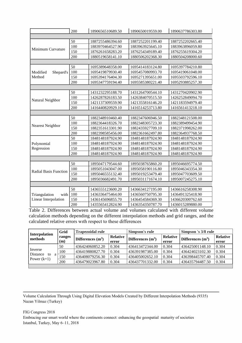
The results of the volumes calculated with different volume calculation methods depending

on the different interpolation methods and grid ranges applied are given in Table 1, and the

differences of these results from the actual volume and the calculated relative errors wıth

respect to these differences are given in Table 2.

Relative Error is given by (8)

estimated actualrelative

actual

V VE

V

(8)

where Erelative is relative error; Vestimated is estimated volume; Vactual is actual volume.

Table 1. The results of the volumes calculated with different volume calculation methods

depending on the different interpolation methods and grid ranges

Interpolation

methods

Grid

ranges

(m)

Volume calculation methods

Trapezoidal rule (m3)

Simpson's rule (m3)

Simpson 's 3/8 rule (m3)

Inverse Distance to a

Power (k=1)

50 1873063892573.60 1873053304065.40 1873064832869.50

100 1873059712549.10 1873031819106.40 1873063854823.70

150 1873047910977.70 1873044834373.50 1873038277428.80

200 1873118855689.20 1873077533053.40 1873075626208.90

Inverse Distance to a

Power (k=2)

50 1874988732022.50 1874983517357.80 1874989438476.00

100 1874983336793.00 1874968392886.10 1874983630882.30

150 1874979095000.20 1874975664864.80 1874975645025.50

200 1875021088515.50 1875008182482.70 1875012230840.70

Kriging

50 1890669126848.40 1890664648539.00 1890669499593.70

100 1890660938849.80 1890665785794.20 1890658667976.40

150 1890663981903.90 1890651355131.90 1890660994133.80



FIG Congress 2018



200 1890656510689.50 1890650019559.00 1890637786303.80

Minimum Curvature

50 1887255486394.60 1887252201199.40 1887252202665.40

100 1883970464527.90 1883963925645.10 1883963896059.80

150 1876261658283.20 1876254349189.40 1876255619304.20

200 1880519658141.10 1880506202368.30 1880504208000.60

Modified Shepard's

Method

50 1695389648358.00 1695414183124.80 1695397784210.80

100 1695419879930.40 1695457080993.70 1695419061048.00

150 1695394176404.30 1695271395651.00 1695503792596.10

200 1695347759194.40 1695585380221.40 1695293885257.30

Natural Neighbor

50 1431232295188.70 1431264700544.10 1431270420902.90

100 1426287826183.50 1426384070515.50 1426252849094.70

150 1421137309559.90 1421355816146.20 1421183594979.40

200 1416440820929.10 1416514253713.80 1416561413218.10

Nearest Neighbor

50 1882348910460.40 1882347606946.50 1882348121508.00

100 1882364418326.70 1882348305723.30 1882389499454.90

150 1882351613301.90 1882435927709.10 1882371998262.00

200 1882398585456.00 1882361662497.80 1882364937768.50

Polynomial

Regression

50 1848148187924.90 1848148187924.90 1848148187924.90

100 1848148187924.90 1848148187924.90 1848148187924.90

150 1848148187924.90 1848148187924.90 1848148187924.90

200 1848148187924.90 1848148187924.90 1848148187924.90

Radial Basis Function

50 1895047179544.60 1895038765860.20 1895046695774.50

100 1895051043047.00 1895058190116.80 1895046343354.30

150 1895046555132.40 1895019253479.40 1895047703609.50

200 1895036682491.70 1895031171674.10 1895007245275.10

Triangulation with

Linear Interpolation

50 1436555123600.20 1436634127195.00 1436616258308.90

100 1436336475464.00 1436560750795.30 1436491325418.90

150 1436145696855.70 1436454584369.30 1436620300762.60

200 1435565412824.90 1436354350787.70 1436015289880.00

Table 2. Differences between actual volume and volumes calculated with different volume

calculation methods depending on the different interpolation methods and grid ranges, and the

calculated relative errors wıth respect to these differences

Interpolation

methods

Grid

ranges

(m)

Trapezoidal rule Simpson's rule Simpson 's 3/8 rule

Differences (m3) Relative

error Differences (m3)

Relative

error Differences (m3)

Relative

error

Inverse

Distance to a

Power (k=1)

50 436424060852.20 0.304 436413472344.00 0.304 436425001148.10 0.304

100 436419880827.70 0.304 436391987385.00 0.304 436424023102.30 0.304

150 436408079256.30 0.304 436405002652.10 0.304 436398445707.40 0.304

200 436479023967.80 0.304 436437701332.00 0.304 436435794487.50 0.304



FIG Congress 2018



Inverse

Distance to a

Power (k=2)

50 438348900301.10 0.305 438343685636.40 0.305 438349606754.60 0.305

100 438343505071.60 0.305 438328561164.70 0.305 438343799160.90 0.305

150 438339263278.80 0.305 438335833143.40 0.305 438335813304.10 0.305

200 438381256794.10 0.305 438368350761.30 0.305 438372399119.30 0.305

Kriging

50 454029295127.00 0.316 454024816817.60 0.316 454029667872.30 0.316

100 454021107128.40 0.316 454025954072.80 0.316 454018836255.00 0.316

150 454024150182.50 0.316 454011523410.50 0.316 454021162412.40 0.316

200 454016678968.10 0.316 454010187837.60 0.316 453997954582.40 0.316

Minimum

Curvature

50 450615654673.20 0.314 450612369478.00 0.314 450612370944.00 0.314

100 447330632806.50 0.311 447324093923.70 0.311 447324064338.40 0.311

150 439621826561.80 0.306 439614517468.00 0.306 439615787582.80 0.306

200 443879826419.70 0.309 443866370646.90 0.309 443864376279.20 0.309

Modified

Shepard's

Method

50 258749816636.60 0.180 258774351403.40 0.180 258757952489.40 0.180

100 258780048209.00 0.180 258817249272.30 0.180 258779229326.60 0.180

150 258754344682.90 0.180 258631563929.60 0.180 258863960874.70 0.180

200 258707927473.00 0.180 258945548500.00 0.180 258654053535.90 0.180

Natural

Neighbor

50 -5407536532.70 -0.004 -5375131177.30 -0.004 -5369410818.50 -0.004

100 -10352005537.90 -0.007 -10255761205.90 -0.007 -10386982626.70 -0.007

150 -15502522161.50 -0.011 -15284015575.20 -0.011 -15456236742.00 -0.011

200 -20199010792.30 -0.014 -20125578007.60 -0.014 -20078418503.30 -0.014

Nearest

Neighbor

50 445709078739.00 0.310 445707775225.10 0.310 445708289786.60 0.310

100 445724586605.30 0.310 445708474001.90 0.310 445749667733.50 0.310

150 445711781580.50 0.310 445796095987.70 0.310 445732166540.60 0.310

200 445758753734.60 0.310 445721830776.40 0.310 445725106047.10 0.310

Polynomial

Regression

50 411508356203.50 0.286 411508356203.50 0.286 411508356203.50 0.286

100 411508356203.50 0.286 411508356203.50 0.286 411508356203.50 0.286

150 411508356203.50 0.286 411508356203.50 0.286 411508356203.50 0.286

200 411508356203.50 0.286 411508356203.50 0.286 411508356203.50 0.286

Radial Basis

Function

50 458407347823.20 0.319 458398934138.80 0.319 458406864053.10 0.319

100 458411211325.60 0.319 458418358395.40 0.319 458406511632.90 0.319

150 458406723411.00 0.319 458379421758.00 0.319 458407871888.10 0.319

200 458396850770.30 0.319 458391339952.70 0.319 458367413553.70 0.319

Triangulation

with Linear

Interpolation

50 -84708121.20 0.000 -5704526.40 0.000 -23573412.50 0.000

100 -303356257.40 0.000 -79080926.10 0.000 -148506302.50 0.000

150 -494134865.70 0.000 -185247352.10 0.000 -19530958.80 0.000

200 -1074418896.50 -0.001 -285480933.70 0.000 -624541841.40 0.000

Relative errors regarding the differences between actual volume value and volume values

obtained with different volume calculation methods according to the different interpolation

methods and grid spacing are shown in Fig. 5, Fig. 6, Fig. 7 and Fig. 8 with bar graphs.



FIG Congress 2018



Fig. 5. Variation of relative errors according to 50 m grid range




FIG Congress 2018



Fig.7. Variation of relative errors according to 150 m grid range




FIG Congress 2018



7. CONCLUSIONS

The volume calculations were made through Surfer8 program. The effects of the parameters

such as, grid range, interpolation methods, volume calculation methods on the volume

calculation was investigated in the study. Moreover, the discussions made taking into account

the amount of relative errors are as follows:

• When the relative errors examined (see Table 2, Figure 5-6-7-8), it was seen that the

most appropriate interpolation model was triangulation with linear. When the relative

errors calculated with other interpolation methods examined, it was seen that the

most appropriate interpolation models were respectively, from smaller to larger,

Natural Neighbor, Modified Shepard's Method, Polynomial Regression, Inverse

Distance to a Power (k=1), Inverse Distance to a Power (k=2), Nearest Neighbor,

Kriging, Radial Basis Function.

• It was seen in the interpolation methods used including minimum curvature, natural

neighbor that the relative errors changed depending on the different grid ranges. In

other methods, the change in grid ranges didn’t affect the relative error.

• Changing the volume calculation methods didn’t affect the relative error. The amount

of relative error wasn’t changed with changing the method of volume calculation.

REFERENCES

[1] Fawzy, H.E. (2015) The Accuracy of Determining the Volumes Using Close Range

Photogrammetry. IOSR Journal of Mechanical and Civil Engineering 2015; 12, Issue 2

Ver. VII, PP 10-15, DOI: 10.9790/1684-12271015.

[2] Chaplot, V., Darboux, F., Bourennane, H., Leguédois, S., Silvera, N. and Phachomphon,

K. (2006) Accuracy of Interpolation Techniques for the Derivation of Digital Elevation

Models in Relation to Landform Types and Data Density. Geomorphology, 77, 126–141,

DOI:10.1016/j.geomorph.2005.12.010.

[3] Bandara, K.R.M.U., Samarakoon, L., Shrestha, R.P. and Kamiya, Y. (2011) Automated

Generation of Digital Terrain Model Using Point Clouds of Digital Surface Model in

Forest Area. Remote Sensing, 3, 845-858, DOI:10.3390/rs3050845.

[4] Heritage, G.L., Milan, D.J., Large, A.R.G. and Fuller, I.C. (2009) Influence of Survey

Strategy and Interpolation Model on DEM Quality. Geomorphology, 112, 334–344,

DOI:10.1016/j.geomorph.2009.06.024.

[5] El-Ashmawy, K.L.A. (2015) A Comparison between Analytical Aerial Photogrammetry,

Laser Scanning, Total Station and Global Positioning System Surveys for Generation of

Digital Terrain Model. Geocarto International, 30, No. 2, 154–162,

http://dx.doi.org/10.1080/10106049.2014.883438.

[6] Schwendel, A.C., Fuller, I.C. and Death, R.G. (2012) Assessing Dem Interpolation

Methods For Effective Representation of Upland Stream Morphology for Rapid

Appraisal of Bed Stability. River Research And Applications, 28, 567–584, DOI:

10.1002/rra.1475.

[7] Zhang, T., Xu, X. and Xu, S. (2015) Method of Establishing an Underwater Digital

Elevation Terrain Based on Kriging Interpolation. Measurement, 63, 287–298,

http://dx.doi.org/10.1016/j.measurement.2014.12.0250263-2241.

[8] Ali, T. and Mehrabian, A. (2009) A Novel Computational Paradigm for Creating a

Triangular Irregular Network (TIN) from LiDAR Data. Nonlinear Analysis, 71, 624-629,

DOI:10.1016/j.na.2008.11.081.



FIG Congress 2018



[9] Hong, W., Chen, T.S. and Chen, J. (2015) Reversible Data Hiding Using Delaunay

Triangulation and Selective Embedment. Information Sciences, 308, 140–154,

http://dx.doi.org/10.1016/j.ins.2014.03.030.

[10] Sangwan, A. and Singh, R.P. (2015) Survey on Coverage Problems in Wireless Sensor

Networks. Wireless Pers Commun, 80, 1475–1500, DOI 10.1007/s11277-014-2094-3.

[11] Surfer 8 software handbook, (2006).

[12] Yanalak, M. (2003) Effect of Gridding Method on Digital Terrain Model Profile Data

Based on Scattered Data. Journal of Computing in Civil Engineering, 17, No. 1, DOI:

10.1061/(ASCE)0887-3801(2003)17:1(58).

[13] Bogusz, J., Kłos, A., Grzempowski, P. and Kontny, B. (2014) Modelling the Velocity

Field in a Regular Grid in the Area of Poland on the Basis of the Velocities of European

Permanent Stations. Pure and Appied Geophysics, 171, 809–833, DOI 10.1007/s00024-

013-0645-2.

[14] Yilmaz, H.M. (2007) The Effect of Interpolation Methods in Surface Definition: An

Experimental Study. Earth Surface Processes and Landforms, 32, 1346–1361, DOI:

10.1002/esp.1473.

[15]Yang, C.S., Kao, S.P., Lee, F.B. and Hung, P.S. (2004) Twelve Different Interpolation

Methods: A Case Study of Surfer 8.0. International Society for Photogrammetry and

Remote Sensing (ISPRS), Volume XXXV, Part B2, Pages 778-785, Istanbul.

[16] Vohat, P., Gupta, V., Bordoloi, T.K., Naswa, H., Singh, G. and Singh, M. (2013)

Analysis of Different Interpolation Methods for Uphole Data Using Surfer Software. 10th

Biennial International Conference & Exposition, Society of Petroleum Geophysicists,

India.

[17] Yakar, M. and Yilmaz, H.M. (2008) Using in Volume Computing of Digital Close Range

Photogrammetry. The International Archives of the Photogrammetry, Remote Sensing

and Spatial Information Sciences, Vol. XXXVII. Part B3b. Beijing 2008.

[18] NETCAD5.0 Software, (1989) NETCAD YAZILIM A.Ş.: NETCAD 5.0 GIS for

WINDOWS, http://www.netcad.com.

BIOGRAPHICAL NOTES

Nazan YILMAZ is a Asist. Prof. Dr. in the Departments of Geomatics Engineering at the

Karadeniz Technical University. She works Geodesy field, expecially physical geodesy, in

this department. She studied about Turkish geoid models in doctorate thesis. She is from

Trabzon of Turkey.

CONTACTS

Title Given name and family name: Asist. Prof. Dr. Nazan YILMAZ

Institution: Karadeniz Technical University

Address: Faculty of Engineering, Department of Geomatics

City: Trabzon

COUNTRY: Turkey

Tel. +90 462 377 37 68

Fax + 90 462 328 09 18

Email: [email protected]

Web site: http://aves.ktu.edu.tr/n_berber/



FIG Congress 2018



volume calculation through using digital elevation models ... · in surfer, three methods are used...

Documents