volume iii – guidelines for microsimulation modeling software
TRANSCRIPT
Volume III – Guidelines for Applying Traffic Microsimulation Modeling Software
finalreport
prepared for
Federal Highway Administration
prepared by
Dowling Associates, Inc.
in association with
Cambridge Systematics, Inc.
August 2003
final report
Volume III – Guidelines for Applying Traffic Microsimulation Modeling Software
prepared for
Federal Highway Administration
prepared by
Dowling Associates, Inc. 180 Grand Avenue, Suite 250 Oakland, California 94612
in association with
Cambridge Systematics, Inc. 555 12th Street, Suite 1600 Oakland, California 94607
August 2003

Volume III – Guidelines for Applying Traffic Microsimulation Modeling Software
Dowling Associates, Inc. & Cambridge Systematics, Inc. i
Quality Assurance Statement
The Federal Highway Administration (FHWA) provides high-quality information to serve Government, industry, and the public in a manner that promotes public understanding. Standards and policies are used to ensure and maximize the quality, objectivity, utility, and integrity of its information. The FHWA periodically reviews quality issues and adjusts its programs and processes to ensure continuous quality improvement.
Volume III – Guidelines for Applying Traffic Microsimulation Modeling Software
Dowling Associates, Inc. & Cambridge Systematics, Inc. iii
Acknowledgements
This material is based upon work supported by the FHWA under contract number DTFH61-01-C-00181.
The California Department of Transportation (Caltrans) Microsimulation Applications Guidelines provided the starting point and initial testing for some of the materials con-tained in this guide. The authors would like to thank Ms. Mary Rose Repine, Mr. Steven Hague, and Mr. Leo Gallagher, all of Caltrans, for their support, comments, and assistance.
Dr. Adolf D. May, of the University of California, Berkeley provided an extensive review of the first draft of this guide.
The Minnesota Department of Transportation’s Advanced CORSIM Training Manual, by Short, Elliott, Hendrickson, Inc., was also a major source of material for this guide.
The microsimulation example problem is based in part on a sample problem used by Mr. Loren Bloomberg, Mr. Mike Swenson, and Mr. Bruce Haldors to compare various simulation models and the Highway Capacity Manual, and draws upon the network coding developed by Mr. Peter Holm. These gentlemen and members of the TRB Committee on Highway Capacity and Quality of Service participated in the development of the original sample problem.
Finally, we would like to acknowledge the extensive contributions to this guide made by the FHWA Traffic Analysis Tools Team: Dr. John Halkias, Dr. Gene McHale, Dr. Henry Lieu, Mr. Grant Zammit, Mr. James McCarthy, Mr. James Colyar, Mr. Michael Schauer, Mr. Chung Tran, Dr. John Tolle, Mr. Edward Fok, Mr. Greg Novak, Mr. James Brachtel, and Ms. Meenakshy Vasudevan.
Richard Dowling Alexander Skabardonis
Dowling Associates, Inc. Oakland, CA
August 25, 2003

Volume III – Guidelines for Applying Traffic Microsimulation Modeling Software
Dowling Associates, Inc. & Cambridge Systematics, Inc. v
Table of Contents
0.0 Introduction .................................................................................................................... 0-1
1.0 Microsimulation Study Organization/Scope............................................................ 1-1 1.1 Study Objectives..................................................................................................... 1-1 1.2 Study Breadth ......................................................................................................... 1-2 1.3 Analytical Approach Selection............................................................................. 1-4 1.4 Analytical Tool Selection (Software) ................................................................... 1-5 1.5 Resource Requirements......................................................................................... 1-6 1.6 Management of a Microsimulation Study .......................................................... 1-8 1.7 Example Problem – Study Scope and Purpose .................................................. 1-9
2.0 Data Collection/Preparation ........................................................................................ 2-1 2.1 Required Data......................................................................................................... 2-2
2.1.1 Geometric Data............................................................................................ 2-2 2.1.2 Control Data ................................................................................................ 2-3 2.1.3 Demand Data............................................................................................... 2-3
2.2 Calibration Data ..................................................................................................... 2-5 2.2.1 Field Inspection ........................................................................................... 2-6 2.2.2 Travel Time Data......................................................................................... 2-6 2.2.3 Point Speed Data......................................................................................... 2-7 2.2.4 Capacity and Saturation Flow Data ......................................................... 2-8 2.2.5 Delay and Queue Data ............................................................................... 2-8
2.3 Data Preparation/Quality Assurance ................................................................. 2-9 2.4 Reconciliation of Traffic Counts........................................................................... 2-10 2.5 Example Problem – Data Collection and Preparation ...................................... 2-10
3.0 Base Model Development ............................................................................................ 3-1 3.1 The Link-Node Diagram – The Model Blueprint .............................................. 3-1 3.2 Link Geometry Data .............................................................................................. 3-4 3.3 Traffic Control Data at Intersections and Junctions .......................................... 3-5 3.4 Traffic Operations and Management Data on Links......................................... 3-5 3.5 Traffic Demand Data ............................................................................................. 3-5 3.6 Driver Behavior Data............................................................................................. 3-6 3.7 Events/Scenarios Data .......................................................................................... 3-6 3.8 Simulation Run Control Data ............................................................................... 3-7 3.9 Coding Techniques for Complex Situations....................................................... 3-7 3.10 Quality Assurance/Control Plan......................................................................... 3-8 3.11 Example Problem – Base Model Development.................................................. 3-8

Volume III – Guidelines for Applying Traffic Microsimulation Modeling Software
vi Cambridge Systematics, Inc.
Table of Contents (continued)
4.0 Error Checking ............................................................................................................... 4-1 4.1 Review Software Errors......................................................................................... 4-1 4.2 Review Inputs......................................................................................................... 4-1 4.3 Review Animation ................................................................................................. 4-2 4.4 Residual Errors ....................................................................................................... 4-4 4.5 Key Decision Point ................................................................................................. 4-5 4.6 Example Problem – Error Checking .................................................................... 4-5
5.0 Calibration of Microsimulation Models ................................................................... 5-1 5.1 Objectives of Calibration....................................................................................... 5-1 5.2 Calibration Approach ............................................................................................ 5-2 5.3 Step One: Calibration for Capacity.................................................................... 5-3
5.3.1 Collect Field Measurements of Capacity ................................................. 5-4 5.3.2 Obtain Model Estimates of Capacity........................................................ 5-5 5.3.3 Select Calibration Parameter(s)................................................................. 5-6 5.3.4 Set Calibration Objective Function........................................................... 5-7 5.3.5 Perform Search for Optimal Parameter Value ........................................ 5-9 5.3.6 Fine-Tune the Calibration.......................................................................... 5-9
5.4 Step 2: Route Choice Calibration ........................................................................ 5-10 5.5.1 Global Calibration....................................................................................... 5-10 5.5.2 Fine-Tuning.................................................................................................. 5-11
5.5 Step 3: System Performance Calibration............................................................ 5-11 5.6 Calibration Targets................................................................................................. 5-11 5.7 Example Problem – Model Calibration............................................................... 5-13
6.0 Alternatives Analysis.................................................................................................... 6-1 6.1 Baseline Demand Forecast .................................................................................... 6-1
6.1.1 Demand Forecasting................................................................................... 6-2 6.1.2 Constraining Demand to Capacity........................................................... 6-2 6.1.3 Allowance for Uncertainty in Demand Forecasts .................................. 6-2
6.2 Generation of Alternatives.................................................................................... 6-2 6.3 Selection of MOEs .................................................................................................. 6-3
6.3.1 Candidate MOEs for Overall System Performance ............................... 6-4 6.3.2 Candidate MOEs for Localized Problems ............................................... 6-4 6.3.3 Choice of Average or Worst Case MOEs................................................. 6-5
6.4 Model Application ................................................................................................. 6-6 6.4.1 Requirement for Multiple Repetitions ..................................................... 6-6 6.4.2 Exclusion of Initialization Period ............................................................. 6-6 6.4.3 Avoiding Bias in the Results ..................................................................... 6-6 6.4.4 Impacts of Alternatives on Demand ........................................................ 6-7 6.4.5 Signal/Meter Control Optimization ........................................................ 6-7

Volume III – Guidelines for Applying Traffic Microsimulation Modeling Software
Dowling Associates, Inc. & Cambridge Systematics, Inc. vii
Table of Contents (continued)
6.5 Tabulation of Results ............................................................................................. 6-7 6.5.1 Reviewing Animation Output .................................................................. 6-8 6.5.2 Numerical Output....................................................................................... 6-9 6.5.3 Correcting Biases in the Results................................................................ 6-9
6.6 Evaluation of Alternatives .................................................................................... 6-12 6.6.1 Interpretation of System Performance Results ....................................... 6-12 6.6.2 Hypothesis Testing ..................................................................................... 6-14 6.6.3 Confidence Intervals and Sensitivity Analysis ....................................... 6-14 6.6.4 Comparison of Results to HCM................................................................ 6-15
6.7 Example Problem – Alternatives Analysis ......................................................... 6-17
7.0 Final Report .................................................................................................................... 7-1 7.1 The Final Report ..................................................................................................... 7-1 7.2 Technical Appendix ............................................................................................... 7-2
Appendix A Traffic Microsimulation Fundamentals
Appendix B Confidence Intervals
Appendix C Estimation of the Simulation Initialization Period
Appendix D Simple Search Algorithms for Calibration
Appendix E Hypothesis Testing of Alternatives
Appendix F Demand Constraints
Appendix G References
Volume III – Guidelines for Applying Traffic Microsimulation Modeling Software
Dowling Associates, Inc. & Cambridge Systematics, Inc. ix
List of Tables
1.1 Milestones and Deliverables for a Microsimulation Study....................................... 1-8
2.1 Vehicle Characteristics Defaults That Can Be Used in Absence of Better Data..... 2-5
3.1 Example Node Numbering Convention...................................................................... 3-4
5.1 Wisconsin DOT Freeway Model Calibration Criteria ............................................... 5-12
5.2 Impact of Queue Discharge Headway on Predicted Saturation Flow .................... 5-14
5.3 System Performance Results for Example Problem................................................... 5-18
6.1 Summary of Analysis Results ....................................................................................... 6-19

Volume III – Guidelines for Applying Traffic Microsimulation Modeling Software
Dowling Associates, Inc. & Cambridge Systematics, Inc. xi
List of Figures
0.1 Microsimulation Model Development and Application Process............................. 0-5
1.1 Prototypical Microsimulation Analysis Task Sequence ............................................ 1-7
1.2 Example Problem Study Network................................................................................ 1-12
3.1 Link-Node Diagram Example....................................................................................... 3-2
3.2 Link-Node Diagram for Example Problem................................................................. 3-9
4.1 Checking Intersection Geometry, Phasing, and Detectors ....................................... 4-7
5.1 Minimization of the Mean Square Error...................................................................... 5-8
5.2 Impact of Mean Queue Discharge Headway on MSE of Modeled Saturation Flow............................................................................................................... 5-14
5.3 Average Speed by Minute of Simulation (Three Links) – Before Calibration........ 5-15
5.4 Average Speed by Minute (Three Links) – After Calibration................................... 5-16
6.1 Computation of Uncaptured Residual Delay at End of Simulation Period ........... 6-11
6.2 Ramp Meter Geometry................................................................................................... 6-18

Volume III – Guidelines for Applying Traffic Microsimulation Modeling Software
Dowling Associates, Inc. & Cambridge Systematics, Inc. 0-1
0.0 Introduction
Microsimulation is the modeling of individual vehicle movements on a second or sub-second basis for the purpose of assessing the traffic performance of highway and street systems, transit, and pedestrians. The last few years have seen a rapid evolution in the sophistica-tion of microsimulation models, and a major expansion of their use in transportation engineering and planning practice. This guidebook provides practitioners with guidance on the appropriate application of microsimulation models to traffic analysis problems, with an overarching focus on an existing and future alternatives analysis.
The use of this guidance will aid in the consistent and reproducible application of microsimulation models, and will further support the credibility of today and tomorrow’s tools. As a result, practitioners and decision-makers will be equipped to make informed decisions that account for the current and evolving technology. Depending on the project-specific purpose, need, and scope, elements of the process described in this guidance may be enhanced or adapted to support the analyst and project team. It is strongly recom-mended that the respective stakeholders and partners consult prior to and throughout the application of any microsimulation model. This further supports the credibility of the results, recommendations, and conclusions, and minimizes the potential for unnecessary or unanticipated tasks.
Organization of Guidebook
This guidebook is organized into the following chapters and appendices:
• Introduction (this chapter) highlights the key guiding principles of microsimulation and provides an overview of the guidebook.
• Chapter 1 addresses the management, scope, and organization of microsimulation analyses.
• Chapter 2 discusses the steps necessary to collect and prepare input data for use in microsimulation models.
• Chapter 3 discusses the coding of input data into the microsimulation models.
• Chapter 4 presents error-checking methods.
• Chapter 5 provides guidance on the calibration of microsimulation models to local traffic conditions.
• Chapter 6 explains how to use microsimulation models for alternatives analysis.

Volume III – Guidelines for Applying Traffic Microsimulation Modeling Software
0-2 Dowling Associates, Inc. & Cambridge Systematics, Inc.
• Chapter 7 provides guidance on the documentation of microsimulation model analysis.
• Appendix A provides an introduction to the fundamentals of microsimulation model theory.
• Appendix B provides guidance on the estimation of the minimum number of microsimulation model run repetitions to achieve a target confidence level and confi-dence interval.
• Appendix C provides guidance on the estimation of the duration of the initialization (“warm-up”) period, after which the simulation has stabilized and it is then appropri-ate to begin gathering performance statistics.
• Appendix D provides examples of some simple manual search algorithms for optimizing parameters during calibration.
• Appendix E summarizes the standard statistical tests that can be used to determine if two alternatives result in significantly different performance. The purpose of these tests is to demonstrate that the improved performance in a particular alternative is not due to random variation in the simulation model results.
• Appendix F describes a manual method for constraining external demands to avail-able capacity. This method is useful for adapting travel demand model forecasts for use in microsimulation models.
• Appendix G provides useful references on microsimulation.
Guiding Principles of Microsimulation
Microsimulation can provide the analyst with a wealth of valuable information on the per-formance of the existing transportation system and potential improvements to it. How-ever, microsimulation can also be a time consuming and resource intensive activity. The key to obtaining a cost-effective microsimulation analysis is to observe certain guiding principles for this type of analysis.
• Use of the appropriate tool is essential. Do not use microsimulation analysis when it is not appropriate. Understand the limitations of the tool and assure yourself that it accurately represents the traffic operations theory. Confirm that it can be applied to support your purpose, needs, scope of work, and can address the question you are asking.
• The Decision Support Methodology for Selecting Traffic Analysis Tools (FHWA, Cambridge Systematics, Inc., August 2003) presents a methodology for selecting the appropriate type of traffic analysis tool for the task at hand.
• Do not use microsimulation if sufficient time and resources are not available. Misap-plication can degrade credibility and be a focus of controversy or disagreement.

Volume III – Guidelines for Applying Traffic Microsimulation Modeling Software
Dowling Associates, Inc. & Cambridge Systematics, Inc. 0-3
• Good data is a “must” for good microsimulation model results.
• It is critical that the analyst calibrate any microsimulation model to local conditions.
• The outputs of a microsimulation model are different than those of the Highway Capacity Manual (HCM). The definitions of key terms, such as delay and queues, are different at the microscopic level of microsimulation models than at the macroscopic level typical of the HCM.
• Prior to embarking on the development of a microsimulation model, establish its scope among partners, reflecting expectations, tasks, and an understanding of how the tool will support the engineering decision. Identify known limitations.
• To minimize disagreements between partners, embed interim periodic reviews at pru-dent milestones in the model development and calibration process.
Additional information on Traffic Microsimulation Fundamentals is provided in Appendix A.
Terminology Used in This Guidebook
• Microsimulation. Microsimulation is the modeling of individual vehicle movements on a second or sub-second basis for the purpose of assessing the traffic performance of highway and street systems.
• Software. Software is a set of computer instructions for assisting the analyst in the development and application of a specific microsimulation model. Several models can be developed using a single software package. These models will share the same basic computational algorithms embedded in the software, but will employ different inputs and parameter values.
• Model. A model is the specific combination of modeling software and the analyst developed inputs/parameters for a specific application. A single model may be applied to the same study area for several time periods and several existing and future improvement alternatives.
• Verification. Verification is the process where the software developer and other researchers check the accuracy of the software implementation of traffic operation the-ory. This guide provides no information on software verification procedures.
• Calibration. Calibration is the process where the analyst selects the model parameters that cause the model to best reproduce field measured local traffic operation conditions.
• Validation. Validation is the process where the analyst checks the overall model pre-dicted traffic performance for a street/road system against field measurements of traf-fic performance, such as traffic volumes, travel times, average speeds, and average delays. Model validation is performed based on field data not used in the calibration process. This guide presumes that the software developer has already completed this

Volume III – Guidelines for Applying Traffic Microsimulation Modeling Software
0-4 Dowling Associates, Inc. & Cambridge Systematics, Inc.
validation of the software and its underlying algorithms in a number of research and practical applications.
• Project. To reduce the chance of confusing the analysis of a project with the project itself, this guide limits its usage of the term “project” to the physical road improve-ment being studied. The evaluation of the impacts of a project will be called an “analysis.”
The Microsimulation Model Development and Application Process
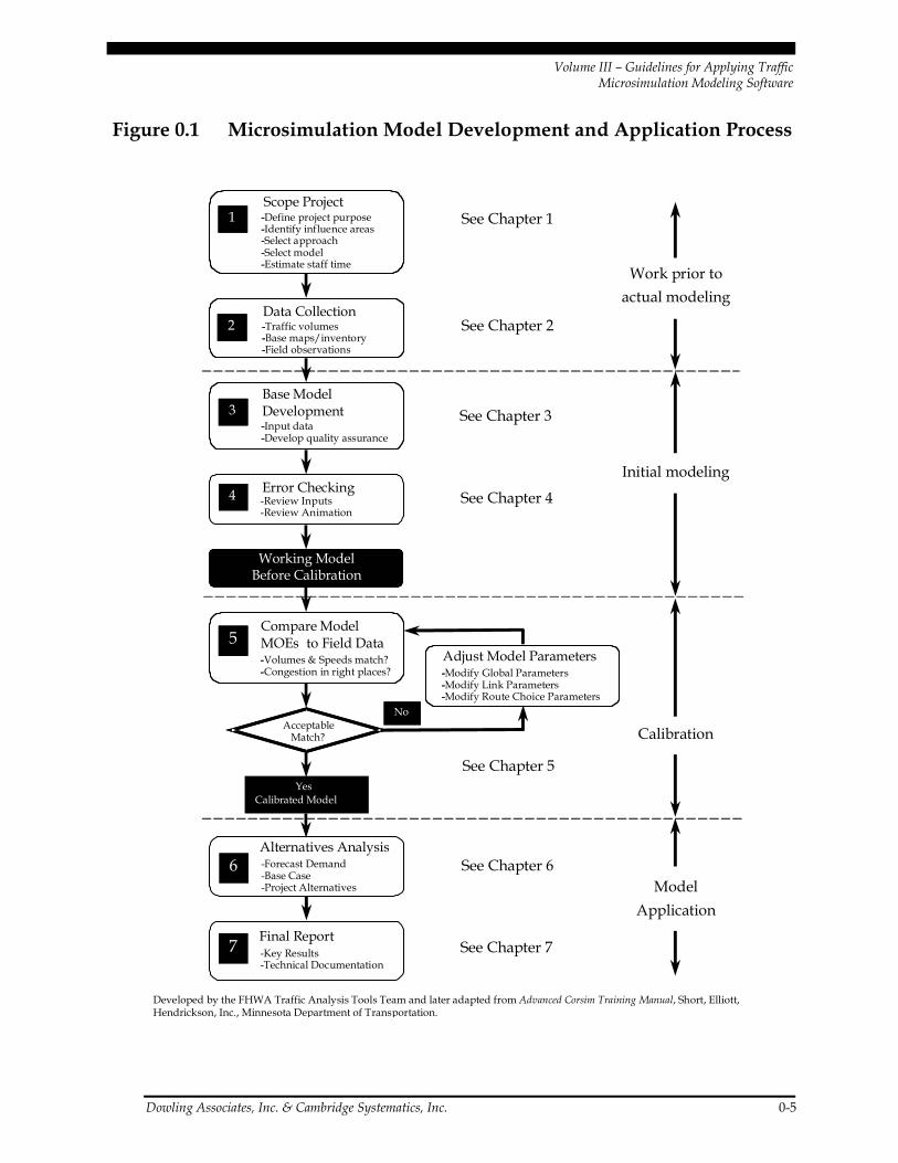
The overall process for developing and applying a microsimulation model to a specific traffic analysis problem consists of seven major tasks:
1. Identification of Study Purpose, Scope, and Approach;
2. Data Collection and Preparation;
3. Base Model Development;
4. Error Checking;
5. Calibration;
6. Alternatives Analysis; and
7. Final Report and Technical Documentation.
Each task is summarized below and described in more detail in subsequent chapters. A flow chart, complementing the overall process, is presented in Figure 0.1. It is intended to be a quick reference that will be traceable throughout the document. This report’s chap-ters correspond to the numbering scheme in Figure 0.1.
To demonstrate the process, an example problem is also provided. The example problem involves the analysis of a corridor consisting of a freeway section and a parallel arterial. For simplicity, this example assumes a proactive traffic management strategy that includes ramp metering. Realizing that each project is unique, the analyst and project manager may realize a need to revisit previous tasks in the process to fully address the issues that arise.
Volume III – Guidelines for Applying Traffic Microsimulation Modeling Software
Dowling Associates, Inc. & Cambridge Systematics, Inc. 0-5
Figure 0.1 Microsimulation Model Development and Application Process
Working ModelBefore Calibration
Working ModelBefore Calibration
4
7
Error Checking
1Scope Project-Define project purpose-Identify influence areas-Select approach-Select model-Estimate staff time
1 -----
2Data Collection-Traffic volumes-Base maps/inventory-Field observations
2 ---
3Base Model Development-Input data-Develop quality assurance
3--
-Review Inputs-Review Animation
See Chapter 1
See Chapter 2
See Chapter 3
See Chapter 4
Work prior toactual modeling
Initial modeling
YesCalibrated Model
5-Volumes & Speeds match?-Congestion in right places?
Compare ModelMOEs to Field Data5--
See Chapter 5
Calibration
-Key Results-Technical Documentation
6 -Forecast Demand-Base Case-Project Alternatives
Alternatives Analysis
-Modify Global Parameters-Modify Link Parameters-Modify Route Choice Parameters
Adjust Model Parameters---
Final Report
AcceptableMatch?
No
See Chapter 6
Developed by the FHWA Traffic Analysis Tools Team and later adapted from Advanced Corsim Training Manual, Short, Elliott, Hendrickson, Inc., Minnesota Department of Transportation.
See Chapter 7
ModelApplication

Volume III – Guidelines for Applying Traffic Microsimulation Modeling Software
0-6 Dowling Associates, Inc. & Cambridge Systematics, Inc.
Task 1. Microsimulation Analysis Organization/Scope
The organization and management of a microsimulation analysis requires the develop-ment of a “scope” for the analysis. This scope includes identification of project objectives, available resources, assessment of verified and available tools, quality assurance plan, and identification of the appropriate tasks to complete the analysis.
The key issues for the management of a microsimulation study are:
• Securing sufficient expertise to develop and/or evaluate the model,
• Providing sufficient time and resources to develop and calibrate the microsimulation model, and
• Developing adequate documentation on the model development process and calibra-tion results.
Task 2 – Data Collection and Preparation
This task involves the collection and preparation of all of the data necessary for the microsimulation analysis. Microsimulation models require extensive input data, including:
• Geometry (lengths, lanes, curvature);
• Controls (signal timing, signs);
• Existing demands (turn volumes, O-D table);
• Calibration data (capacities, travel times, queues); and
• Transit, bicycle, and pedestrian data.
In support of Tasks 4 and 5, current and accurate data required for error checking and calibration should also be collected. While capacities can be measured at anytime, it is crucial that the other calibration data (travel times, delays, and queues) be gathered simultaneously with the traffic counts.
Task 3 – Base Model Development
The goal of base model development is a model that is verifiable, reproducible, and accu-rate. It is a complex and time-consuming task with steps that are specific to the software used to perform the microsimulation analysis. The details of model development are best covered in software specific users’ guides, and, for this reason, the development process may vary. This guide provides a general outline of the model development task.
The method for developing a microsimulation model can be best thought of as the building up of several “layers” of the model until the model is completed. The first layer, the link/node diagram, sets the foundation for the model. Additional data on traffic controls and link operations are then added on top of this foundation. Travel demand and traveler

Volume III – Guidelines for Applying Traffic Microsimulation Modeling Software
Dowling Associates, Inc. & Cambridge Systematics, Inc. 0-7
behavior data are then added to the basic network. Finally, the simulation run control data are input to complete the model development task. The model development process does not have to follow this order exactly, but each of these layers is required in some form in any simulation model. The model development task should also include the development and implementation of a quality assurance/control (QA/QC) plan to reduce the introduction of input coding errors into the model.
Task 4 – Error Checking
The error-checking task is necessary to identify and correct model coding errors, so that they do not interfere with the model calibration task. Coding errors can distort the model calibration process and cause the analyst to adopt incorrect values for the calibration parameters. Error checking involves various tests of the coded network and the demand data to identify input coding errors.
Task 5 – Microsimulation Model Calibration
Each microsimulation software package has a set of user-adjustable parameters that enable the practitioner to calibrate the software to better match specific local conditions. These parameter adjustments are necessary because no microsimulation model can include all of the possible factors (both on-street and off-street) that might affect capacity and traffic operations. The calibration process accounts for the impacts of these “un-modeled” site-specific factors through the adjustment of calibration parameters included in the soft-ware for this specific purpose.
Model calibration, therefore, involves the selection of a few parameters for calibration and the repeated operation of the model to identify the best values for those parameters. This can be a time-consuming process. It should be well documented, so that later reviewers of the model can understand the rationale for the various parameter changes made during calibration. For example, the car-following sensitivity factor for a specific freeway seg-ment (link 20-21) has been modified to the value of 95 to match the observed average speed in this freeway segment.
The key issues in calibration are:
• Identification of necessary model calibration targets;
• Allocation of sufficient time and resources to achieve calibration targets;
• Selection of the appropriate calibration parameter values to best match locally meas-ured street, highway, freeway, and intersection capacities;
• Selection of calibration parameter values that best reproduce current route choice pat-terns; and
• Calibration of the overall model against overall system performance measures, such as travel time, delay, and queues.

Volume III – Guidelines for Applying Traffic Microsimulation Modeling Software
0-8 Dowling Associates, Inc. & Cambridge Systematics, Inc.
Task 6 – Alternatives Analysis with Microsimulation Models
This is the first model application task. The calibrated microsimulation model is run sev-eral times to test various project alternatives. The first step in this task is to develop a baseline demand scenario. Then the various improvement alternatives are coded into the simulation model. The analyst then determines which performance statistics will be gath-ered and runs the model for each alternative to generate the necessary output. If the ana-lyst wishes to produce HCM level of service (LOS) results, then sufficient time should be allowed for post-processing the model outputs to convert microsimulation results into HCM-compatible LOS results.
The key issues in an alternatives analysis are:
• Forecasting realistic future demands,
• Selection of the appropriate performance measures for evaluation of the alternatives,
• Accurate accounting of the full congestion reduction benefits of each alternative, and
• Proper conversion of microsimulation results to HCM LOS (reporting LOS is optional).
Task 7 – Final Report/Technical Documentation
This task involves summarization of the analytical results in a final report and documen-tation of the analytical approach in a technical document. This task may also include presentation of study results to technical supervisors, elected officials, and the general public.
The final report presents the analytical results in a form readily understandable to the decision-makers for the project. The effort involved in summarization of the results for the final report should not be under-estimated, since microsimulation models produce a wealth of numerical output that must be tabulated and summarized.
Technical documentation is important for ensuring that the decision-makers understand the assumptions behind the results, and for enabling other analysts to reproduce the results. The documentation should be sufficient, so that given the same input files, another analyst can understand the calibration process and repeat the alternatives analysis.

Volume III – Guidelines for Applying Traffic Microsimulation Modeling Software
Dowling Associates, Inc. &Cambridge Systematics, Inc. 1-1
1.0 Microsimulation Study Organization/Scope
Microsimulation can provide a wealth of information, but it can also be a very time-consuming and resource intensive effort. It is critical that the manager effectively manage the microsimulation effort to ensure a cost-effective outcome to the study. The primary component of an effective management plan is the study scope, which defines the objec-tives, breadth, approach, tools, resources, and time schedule for the study. This chapter presents the key components of an overall management plan for achieving a cost-effective microsimulation analysis.
1.1 Study Objectives
Before embarking on any major analytical effort, it is wise to assess exactly what it is the analyst, manager, and decision-makers hope to accomplish. One should identify the study objectives, the breadth of the study, and the appropriate tools and analytical approach to accomplish those objectives.
Study objectives should answer the following questions:
• Why is the analysis needed?
• What questions should the analysis answer? (What alternatives will be analyzed?)
• Who are the intended recipients/decision-makers for the results?
Try to avoid broad, all encompassing study objectives. They are difficult to achieve with the limited resources normally available, and they do not help focus the analysis on the top priority needs of the analysis. It can save a great deal of study resources if the man-ager and analyst can identify up front what the analysis will NOT achieve. The objectives for the analysis should be realistic, recognizing the resources and time that may be avail-able for their achievement.
Precise study objectives will ensure a cost-effective analysis.
It can be just as useful to identify what will NOT be analyzed, as it is to identify what WILL be analyzed.

Volume III – Guidelines for Applying Traffic Microsimulation Modeling Software
1-2 Dowling Associates, Inc. & Cambridge Systematics, Inc.
1.2 Study Breadth
Once the study objectives have been identified, the next step is to identify the scope or breadth of the analysis, the geographic and temporal bounds of the analysis. Several questions related to the required breadth of the analysis should be answered at this time.
• What are the characteristics of the project being analyzed? How large and complex is it?
• What are the alternatives to be analyzed? How many, how large, and how complex are they?
• What measures of effectiveness (MOEs) will be required to evaluate the alternatives, and how can they be measured in the field?
• What resources are available to the analyst?
• What are the likely geographic and temporal scopes of the impacts of the project and its alter-natives (now and in the future)? How far and for how many hours does the congestion extend? The geographic and temporal bounda-ries selected for the analysis should encompass all of the expected congestion, so as to provide a valid basis for comparing alternatives.1
• What degree of precision do the decision-makers require? Is 10 percent error toler-able? Are hourly averages satisfactory? Are the impacts of the alternatives likely to be very similar or very different from those of the proposed project? How disaggregate of an analysis is required? Is the analysis likely to produce a set of alternatives where the decision-makers must choose between varying levels of congestion – as opposed to the situation where one or more alternatives eliminate congestion, while others do not?
Developing a logical terminus of an improvement project versus a model has been debated since the early days of microsimulation; in the end, it boils down to balancing
1 The analyst should try to design the model to geographically and temporally encompass all
significant congestion to ensure that the model is evaluating demands rather than capacity; however, the extent of congestion in many urban areas and resource limitations may preclude 100 percent achievement of this goal. If this goal cannot be 100 percent achieved, then the analyst should attempt to encompass as much of the congestion as is feasible within the resource constraints and be prepared to post-process the model’s results to compensate for the portion of congestion not included in the model.
The geographic and temporal scope of a microsimulation model should be sufficient to completely encompass all of the traffic congestion present in the primary influence area of the project during the target analysis period.

Volume III – Guidelines for Applying Traffic Microsimulation Modeling Software
Dowling Associates, Inc. &Cambridge Systematics, Inc. 1-3
study objectives and study resources. Therefore, the modeler needs to understand the operation of the improvement project in order to develop logical termini.
The study termini will be dependent on the “zone of influence,” and the project manager will likely make that determination in consultation with the project stakeholders. Once that is completed, then the modeler needs to take off from there and look at the operation of that proposed facility. When determining the “zone of influence,” the modeler needs to understand operational characteristics of the facility of the proposed project. This could be one intersection beyond the project terminus at one end of the project or a major gen-erator two miles away from the other end of the project. Therefore, there is no geographi-cal guidance that can be given. However, some general “rules of thumb” are summarized as follows:
• Interstate projects. The model network should extend 1.5 miles from both termini of the improvement being evaluated and one mile on either side of the interstate route.
• Arterial projects. The model network should extend two intersections beyond those within the bound of the improvement, and consider potential impacts to arterial coor-dination as warranted.
The model study area should include areas that might be impacted by the proposed improvement strategies. For example, if an analysis is to be conducted of incident man-agement strategies, the model study area should include the area impacted by the diverted traffic. All potential problem areas should be included in the model network. For example, if queues are identified in the network boundary areas, the analyst might need to extend the network further upstream.
A study scope that has a tight geographic focus, lit-tle tolerance for errors, and little difference in the performance of the alternatives will tend to point to microsimulation as the most cost-effective approach2. A scope with a moderately greater geo-graphic focus and with a 20 years in the future timeframe will tend to require a blended travel demand model and microsimulation approach. A scope that covers large geographic areas and long timeframes in the future will tend to rule out microsimulation and require instead a combination of travel demand models and HCM analysis techniques.
2 Continuing improvements in data collection, computer technology, and software will eventually
enable microsimulation models to be applied to larger problems.
Microsimulation is like a microscope. It is a very effective tool when you have it pointed at the correct subject. Tightly focused scopes of work ensure cost-effective microsimulation analyses.

Volume III – Guidelines for Applying Traffic Microsimulation Modeling Software
1-4 Dowling Associates, Inc. & Cambridge Systematics, Inc.
1.3 Analytical Approach Selection
The Decision Support Methodology for Selecting Analysis Tools3 (a separate document) pro-vides detailed guidance on the selection of an appropriate analytical approach. This sec-tion provides a brief summary of the key points.
Microsimulation takes more effort than macroscopic simulation, and macroscopic simulation takes more effort than HCM-type analyses. The analyst should employ only the level of effort required by the problem being studied.
The following are several situations where microsimulation is the best technical approach for performing a traffic analysis:
• Conditions that violate the basic assumptions of other available analytical tools,
• Conditions not covered by other available analytical tools, and
• Testing of vehicle performance, guidance, and driver behavior modification options.
For example, most of the HCM procedures assume that the operation of one intersection or road segment is not adversely affected by conditions on the adjacent roadway.4 Long queues from one location interfering with another location would violate this assumption. Microsimulation would be the superior analytical tool for this situation.
Microsimulation models, because they are sensitive to different vehicle performance char-acteristics and differing driver behavior characteristics, are useful for testing Intelligent Transportation Systems (ITS) strategies designed to modify these characteristics. Traveler information systems, automated vehicle guidance, triple or quadruple trailer options, new weight limits, new propulsion technologies, etc. are all excellent candidates for testing with microsimulation models. The HCM procedures, for example, are not designed to be sensitive to new technology options, while microsimulation allows one to predict what the effect of new technology might be on capacity before the new technology is actually in place.
3 Cambridge Systematics, Inc. and Dowling Associates, Decision Support Methodology for Selecting
Analysis Tools, FHWA, Washington, D.C., 2003, available on the web at http://ops.fhwa.dot.gov/Travel/Traffic_Analysis_Tools/traffic_analysis_tools.htm.
4 The one exception to this statement is the recently developed Freeway Systems analysis methodology presented in the Year 2000 HCM, which does explicitly treat oversaturated flow situations.
Microsimulation models are data intensive. They should be used only when sufficient resources can be made available and less data-intensive approaches cannot yield satisfactory results.

Volume III – Guidelines for Applying Traffic Microsimulation Modeling Software
Dowling Associates, Inc. &Cambridge Systematics, Inc. 1-5
Software selection is like picking out a suit of clothes. There is no single suit that fits all people and all uses. You must know what your software needs are and the capabilities and training of the people that you expect to use the software. Then you can select the software that best meets your needs and best fits the capabilities of the people that will use it.
1.4 Analytical Tool Selection (Software)
The selection of the appropriate analytical tool is a key part of the study scope and tied into the selec-tion of the analytical approach. The key criteria for software selection are technical capabilities, input/output/interfaces, user training/support, and ongoing software enhancements5.
Generally, it is a good idea to decouple the selection of the appropriate analysis tool from the actual implementation of the tool. This can be accomplished by identifying a separate task in the Scope of Work for selecting the appropriate analysis tool based on a set of criteria. The FHWA’s Decision Support Methodology for Selecting Traffic Analysis Tools document identifies several criteria that should be considered in the selection of an appropriate traffic analysis tool and helps identify the circumstances when a particular type of tool should be used. A methodology also is presented to guide the users in the selection of the appropriate tool category. This document includes worksheets that transportation professionals can utilize to select the appropriate tool category, and assistance to identify the most appropriate tool within the selected category. An automated tool that implements this methodology can be found at the FHWA Traffic Analysis Tools web site at:
http://ops.fhwa.dot.gov/Travel/Traffic_Analysis_Tools/traffic_analysis_tools.htm
Technical Capabilities
The technical capabilities of the software relate to its ability to accurately forecast the traf-fic performance of the alternatives being considered in the analysis. The manager must decide if the software is capable of handling the size of problems being evaluated in the study. Are the technical analysis procedures incorporated in the software sensitive to the variables of concern in the study? The following is a general list of technical capabilities to be considered in software selection:
• Maximum problem size (the software may be limited by the maximum number of sig-nals that can be in a single network, or the maximum number of vehicles that may be present on the network at any one time);
5 A more complete discussion of software selection criteria can be found in J. W. Shaw and
D. H. Nam, Microsimulation, Freeway System Operational Assessment, and Project Selection in Southeastern Wisconsin: Expanding the Vision, paper presented at Transportation Research Board (TRB) Annual Meeting, Washington, D.C., 2002.

Volume III – Guidelines for Applying Traffic Microsimulation Modeling Software
1-6 Dowling Associates, Inc. & Cambridge Systematics, Inc.
• Vehicle movement logic (lane changing, car following, etc.) that reflects the state-of-the-art;
• Sensitivity to specific features of the alternatives being analyzed (such as trucks on grades, effects of horizontal curvature on speeds, or advanced traffic management techniques);
• Model parameters available for model calibration; and
• The manager should consider the variety and extent of prior successful applications of the software package.
Input/Output/Interfaces
Input, output, and the ability of the software to interface with other software that will be used in the study (such as traffic forecasting models) are other key considerations. The manager should review the ability of the software to produce reports on the MOEs needed for the study. The ability to customize output reports can also be very useful to the analyst.
It is essential that the manager or analyst understand the definitions of the MOEs, as defined by the software. This is because a given MOE may be calculated or defined dif-ferently by the software, as compared to how it is defined or calculated by the HCM.
User Training/Support
User support and training requirements are another key consideration. What kind of training and support is available? Are their other users in the area that can provide informal advice?
Ongoing Software Enhancements
Finally, the commitment of the software developer to ongoing enhancements ensures that the agency’s investment in staff training and model development in a particular software tool will continue to pay off over the long term. Unsupported software can become unus-able as operating systems and hardware advance.
1.5 Resource Requirements
The resource requirements for the development, calibration, and application of microsimulation models will vary according to the complexity of the project, its geo-

Volume III – Guidelines for Applying Traffic Microsimulation Modeling Software
Dowling Associates, Inc. &Cambridge Systematics, Inc. 1-7
graphic scope, its temporal scope, the number of alternatives, and the availability and quality of data6.
In terms of training, the person responsible for the initial round of coding can be a begin-ner or intermediate level in terms of knowledge of the software. They should have supervision from an individual with more experience with the software. Error checking and calibration are best done by a person with advanced knowledge of the microsimula-tion software and underlying algorithms. Model documentation and public presentations can be done by a person with intermediate level of knowledge of microsimulation software.
A prototype time schedule for the various model development, calibration, and applica-tion tasks is presented in Figure 1.1, which shows the sequential nature of the task and their relative durations. Data collection, coding, error checking, and calibration are the critical path tasks to completing a calibrated model. The alternatives analysis cannot be started until the calibrated model has been reviewed and accepted.
Figure 1.1 Prototypical Microsimulation Analysis Task Sequence
Task
1. Project Scope
2. Data Collection
3. Develop Base Model
4. Error Checking
5. Calibration
6. Alternatives Analysis
7. Final
Project Schedule
6 Some managers might devote about 50 percent of the budget to the tasks that lead up to and
include coding of the simulation model, including data collection. Another 25 percent of the budget might go to calibration. The remaining 25 percent might then go to alternatives analysis and documentation. Others might divide the resources into one-third for data collection and model coding, one-third for calibration, and one-third for alternatives analysis and documentation.

Volume III – Guidelines for Applying Traffic Microsimulation Modeling Software
1-8 Dowling Associates, Inc. & Cambridge Systematics, Inc.
1.6 Management of a Microsimulation Study
Much of the management of a microsimulation study is the same as managing any other highway design project: establish clear objectives, define a solid scope of work and schedule, monitor milestones, and review deliverables. The key milestones and deliver-ables for a microsimulation study are shown in Table 1.1.
Table 1.1 Milestones and Deliverables for a Microsimulation Study
Milestone Deliverable Contents 1. Study scope 1. Study scope and schedule
2. Proposed data collection plan 3. Proposed calibration plan 4. Coding quality assurance plan
Identifies study objectives, geographic and temporal scope, alternatives, data collection plan, coding error-checking procedures, calibration plan and targets
2. Data collection 5. Data collection results report Data collection procedures, quality assurance, summary of results
3. Model development
6. 50% coded model Software input files
4. Error checking 7. 100% coded model Software input files
5. Calibration 8. Calibration test results report Calibration procedures, adjusted parameters and rationale, achievement of calibration targets
6. Alternatives analysis
9. Alternatives analysis report Description of alternatives, analysis procedures, results
7. Final report 10. Final Report Summary tables and graphics highlighting key results
11. Technical Documentation Compilation of prior reports documenting model development and calibration, software input files
Two problems are often encountered when managing microsimulation models developed by others, including:
1. Insufficient managerial expertise to verify the technical application of the model; and
2. Insufficient data/documentation to calibrate the model.

Volume III – Guidelines for Applying Traffic Microsimulation Modeling Software
Dowling Associates, Inc. &Cambridge Systematics, Inc. 1-9
The study manager may choose to bring more expertise to the review of the model by forming a technical advisory panel. Furthermore, utilization of a panel may support a project of regional importance and detail, or address stakeholder interest regarding the acceptance of new technology. The panel may be drawn from experts at other public agencies, consultants, or a nearby university. The experts should have had prior experi-ence developing simulation models with the specific software being used for the particu-lar model.
The manager (and the technical advisory panel) must have access to the input files and the software for the microsimulation model. There are several hundred parameters involved in the development and calibration of a simulation model. Consequently, it is impossible to assess the technical validity of a model based solely upon its printed output and visual animation of the results. The manager must have access to the model input files, so that he or she can assess the veracity of the model by reviewing the parameter values that go into the model, as well as looking at its output.
Finally, good documentation of the model calibration process and rationale for parameter adjustments is required so that the technical validity of the calibrated model can be assessed. A standardized format for the calibration report can expedite the review process.
1.7 Example Problem – Study Scope and Purpose
The example problem is a study of the impacts of freeway ramp metering on freeway and surface street operations. The ramp metering will be operational during the afternoon peak period on the eastbound on-ramps at two interchanges7.
Study objectives. To quantify the traffic operation benefits and impacts of the proposed p.m. peak period ramp metering project on both the freeway and nearby surface streets. The information will be provided to technical people at both the State Department of Transportation (DOT) and City Public Works Department.
Study breadth (geographic). The ramp meter project is expected to impact freeway and surface street operations several miles upstream and downstream of the two metered on-ramps. However, the most significant impacts are expected in the immediate vicinity of the meters (the two interchanges, the closest parallel arterial streets, and the cross-connector streets between the interchanges and the parallel arterial). If the negative
7 This example problem is part of a larger project involving metering of several miles of freeway.
The study area in the example problem was selected to illustrate the concepts and procedures in the microsimulation guide.
Volume III – Guidelines for Applying Traffic Microsimulation Modeling Software
1-10 Dowling Associates, Inc. & Cambridge Systematics, Inc.
impacts of the ramp meters are acceptable in the immediate vicinity of the project, then they should be of a lower magnitude and, therefore, also acceptable farther away8.
There is no parallel arterial street north of the freeway, so only the parallel arterial on the south side needs to be studied. Figure 1.2 illustrates the selected study area. There are six signalized intersections along the study section of Green Bay Avenue parallel arterial. The signals are operating on a common 90-second cycle length. The signals at the ramp junc-tions on Wisconsin and Milwaukee also operate on a 90-second cycle length.
The freeway and adjacent arterial are currently uncongested during the p.m. peak period and, consequently, the study area need only be enlarged to encompass projected future congestion. The freeway and arterial are modeled one mile east and west of the two inter-changes to include possible future congestion under the “no-meter” and “meter” alternatives.
Study breadth (temporal). Since there is no existing congestion on the freeway and sur-face streets, and the ramp metering will occur only in the p.m. peak hour, the p.m. peak hour is selected as the temporal bounds for the analysis9.
Analytical approach. There are concerns that 1) freeway traffic may be diverted to city streets causing unacceptable congestion, and 2) traffic at metered on-ramps may back up and adversely impact surface street operations. A regional travel demand model would probably not be adequate to estimate traffic diversion due to a regional ramp metering system, because it could not model site- and time-specific traffic queues accurately and would not be able to predict the impacts of the meters on surface street operations. HCM methods could estimate the capacity impacts of ramp metering, but, because these meth-ods are not well adapted to estimating the impacts of downstream congestion on upstream traffic operations, they are not sufficient by themselves for the analysis of the impacts of ramp meters on surface street operations. Microsimulation would likely assist the analyst at predicting traffic diversions between the freeway and surface streets and would be the appropriate analytical tool for this problem.
Analytical tool. The analyst selects a microsimulation tool that either incorporates a pro-cedure for rerouting of freeway traffic in response to ramp metering, or the analyst sup-plements the microsimulation tool with a separate travel demand model analysis to predict rerouting of traffic10.
8 Of course, if the analyst does not believe this to be true, then the study area should be expanded
accordingly. 9 If existing or future congestion on either the freeway or arterial were expected to last more than
one hour, then the analysis period would be extended to encompass all of the existing and future congestion in the study area.
10 For this example problem, a microsimulation tool without rerouting capabilities was selected. It was supplemented with estimates of traffic diversions from a regional travel demand model.

Volume III – Guidelines for Applying Traffic Microsimulation Modeling Software
Dowling Associates, Inc. &Cambridge Systematics, Inc. 1-11
Resource requirements and schedule. The resource requirements and schedule are esti-mated at this time to ensure that the project can be completed with the selected approach to the satisfaction of the decision-makers. Details of resources and schedule are not dis-cussed here because they are specific to the resources available to the analyst and the timeline available for completion.

Volume III – Guidelines for Applying Traffic Microsimulation Modeling Software
1-12 Dowling Associates, Inc. & Cambridge Systematics, Inc.
Figure 1.2 Example Problem Study Network
Green Bay
Mainline USA
Wis
cons
in
Milw
auke
e
1stSt
reet
3rd
Stre
et
4th
Stre
et
6th
Stre
et

Volume III – Guidelines for Applying Traffic Microsimulation Modeling Software
Dowling Associates, Inc. &Cambridge Systematics, Inc. 2-1
2.0 Data Collection/Preparation
This chapter provides guidance on the identification, collection, and preparation of the data sets needed to develop a microsimulation model for a specific project analysis, and the data needed to evaluate the calibration and fidelity of the model to ‘real-world’ conditions pre-sent in the project analysis study area. There are agency-specific techniques and guidance documents that focus on data collection, which should be utilized to support project-specific needs.
A selection of general guides on the collection of traffic data includes:
• Introduction to Traffic Engineering: A Manual for Data Collection and Analysis, T. R. Currin, Brooks/Cole, 2001, 140 pp., ISBN No: 0-534378-67-6;
• Manual of Traffic Engineering Studies, P. C. Box, J. C. Oppenlander, Institute of Transportation Engineers, Washington, D.C., 1983; and
• Highway Capacity Manual 2000, TRB, 2000, 1200 pp., ISBN No.: 0-309067-46-4.
These sources should be consulted regarding appropriate data collection methods, and are not all-inclusive on the subject of data collection. The discussion in this chapter focuses on data requirements, potential data sources, and the proper preparation of data for use in microsimulation analysis.
If the amount of available data does not adequately support the project objectives and scope identified in Task 1, then the project team should return to Task 1 and re-define the objectives and scope so that they will be sufficiently supported by the available data.
Working ModelBefore Calibration
4
7
Error Checking
1 Scope Project
2 Data Collection
3 Base Model Development
Work prior toactual modeling
Initial modeling
YesCalibrated Model
5Compare ModelMOE’s to FieldData
Calibration
6 Alternatives Analysis
Adjust Model Parameters
Final Report
AcceptableMatch?
No
ModelApplication

Volume III – Guidelines for Applying Traffic Microsimulation Modeling Software
2-2 Dowling Associates, Inc. & Cambridge Systematics, Inc.
2.1 Required Data
The precise input data required by a microsimulation model will vary by software and the specific modeling application as defined by the study objectives and scope. Most microsimulation analysis studies will require the following types of input data11:
1. Road geometry (lengths, lanes, curvature);
2. Traffic controls (signal timing, signs);
3. Demands (entry volumes, turn volumes, O-D table); and
4. Calibration data (traffic counts and performance data such as speed, queues).
In addition to the above basic input data, microsimulation models also require data on vehicle and driver characteristics (vehicle length, maximum acceleration rate, driver aggressiveness, etc.). Because these data can be difficult to measure in the field, it is often supplied with the software in the form of various default values.
Each microsimulation model will also require various control parameters that specify how the model conducts the simulation. The user’s guide for the specific simulation software should be consulted for a complete list of input requirements. The discussion below describes only the most basic data requirements shared by the majority of microsimula-tion model software.
2.1.1 Geometric Data
The basic geometric data required by most models consists of the number of lanes, length, and free-flow speed12. For intersections, the necessary geometric data may also include the designated turn lanes and their vehicle storage lengths. This data can usually be obtained from construction drawings, field surveys, geographical information systems (GIS) files, or aerial photos.
11 The forecasting of future demands (turn volumes, OD table) is discussed later under the
Alternatives Analysis task. 12 Some microsimulation models may allow (or require) the analyst to input additional geometric
data related to the grades, horizontal curvature, load limits, height limits, shoulders, on-street parking, pavement condition, etc.

Volume III – Guidelines for Applying Traffic Microsimulation Modeling Software
Dowling Associates, Inc. &Cambridge Systematics, Inc. 2-3
2.1.2 Control Data
Control data consist of the locations of traffic control devices and signal timing settings13. This data can best be obtained from the files of the agencies operating the traffic controls, or from field inspection.
2.1.3 Demand Data
The basic travel demand data required for most models consist of entry volumes (traffic entering the study area) and turn movements at intersections within the study area. Some models require one or more vehicular O-D tables, which enable the modeling of route diversions. Procedures exist in many demand modeling software and some microsimula-tion software for estimating O-D tables from traffic counts.
Count Locations and Duration
Traffic counts should be conducted at key locations within the microsimulation model study area for the duration of the proposed simulation analysis period. The counts should ideally be aggregated to no longer than 15-minute time periods, but alternative aggrega-tions can be used if dictated by circumstances14.
If congestion is present at a count location (or upstream of it), care should be taken to ensure that the count measures “demand” and not capacity. The count period should ide-ally start before the onset of congestion and end after the dissipation of all congestion to ensure that all queued demand is eventually included in the count.
The counts should be conducted simultaneously if resources permit so that all count information is consistent with a single simulation period. Often, resources do not permit this for the larger simulation areas, so the analyst must establish one or more control sta-tions where a continuous count is maintained over the length of the data collection period. The analyst then uses the control station counts to adjust the counts collected over several days into a single, consistent set of counts representative of a single “typical” day within the study area.
13 Some models may allow the inclusion of advanced traffic control features. Some models require
the equivalent fixed time inputs for traffic-actuated signals. Others can work with both fixed time and actuated controller settings.
14 Project constraints, traffic counter limitations, or other considerations (such as a long simulation period) may require that counts be aggregated to longer or shorter periods.

Volume III – Guidelines for Applying Traffic Microsimulation Modeling Software
2-4 Dowling Associates, Inc. & Cambridge Systematics, Inc.
Estimating Origin-Destination Trip Tables
For some simulation software, the counts must be converted into an estimate of existing O-D trip patterns. Other software can work with either turn movement counts or an O-D table. An O-D table is required if it is desired to model route choice shifts within the microsimulation model.
Local metropolitan planning organization (MPO) travel demand models can provide O-D data, but these data sets are generally limited to the nearest decennial Census year and the zone system is usually too macroscopic for microsimulation. The analyst must usually estimate the existing O-D table from the MPO O-D data in combination with other data sources, such as traffic counts. This process will likely require a consideration of O-D pattern changes due to time of day; especially for simulations that cover an extended period of time throughout the day.
A license plate matching survey is the most accurate method for measuring existing O-D data. The analyst establishes checkpoints within and on the periphery of the study area and notes the license plate numbers of all vehicles passing by each checkpoint. A matching program then is used to determine how many vehicles traveled between each pair of checkpoints. License plate surveys, however, can be quite expensive. For this reason, the estimation of the O-D table from traffic counts is often selected15.
Vehicle Characteristics
The vehicle characteristics typically include vehicle mix, vehicle dimensions, and vehicle performance characteristics (maximum acceleration, etc.).16
Vehicle mix. The vehicle mix is defined by the analyst, often in terms of the percentage of total vehicles generated in the O-D process. Typical vehicle types in the vehicle mix might be passenger cars, single-unit trucks, semi-trailer truck, and bus.
Default percentages are usually included in most software packages, but the vehicle mix is something that is highly localized, and national default values will rarely be valid for spe-cific locations. For example, the percentage of trucks in the vehicle mix can vary from a low of two percent on urban streets during rush hour to a high of 40 percent of daily weekday traffic on an intercity interstate freeway.
15 There are many references in the literature on the estimation of O-D from traffic counts.
Appendix A, Chapter 29, of the HCM (Year 2000 edition) provides a couple of simple O-D estimation algorithms. Most travel demand software and some microsimulation software have O-D estimation modules available.
16 The software-supplied default vehicle mix, dimensions, and performance characteristics should be reviewed to ensure that they are representative of local vehicle fleet data, especially for simulation software developed outside the United States.

Volume III – Guidelines for Applying Traffic Microsimulation Modeling Software
Dowling Associates, Inc. &Cambridge Systematics, Inc. 2-5
It is recommended that the analyst obtain one or more vehicle classification studies for the study area for the time period being analyzed. Vehicle classification studies can often be obtained from nearby truck weigh station locations.
Vehicle dimensions and performance. The analyst should attempt to obtain the vehicle fleet data (vehicle mix, dimensions, and performance) from the local state DOT or air quality management agency. National data can be obtained from Motor and Equipment Manufacturers Association, various car manufacturers, the FHWA, and the Environmental Protection Agency (EPA). In the absence of data from these sources, the analyst may use the defaults shown in Table 2.1.
Table 2.1 Vehicle Characteristics Defaults That Can Be Used in Absence of Better Data
Vehicle Type Length (ft) Max. Speed
(mph) Max. Accel.
(ft/ sec2) Max. Dec. (ft/sec2)
Jerk (ft/sec3)
Passenger cars 14 75 10 15 7
Single-unit truck 35 75 5 15 7
Semi-trailer truck 53 67 3 15 7
Double-bottom trailer truck
64 61 2 15 7
Bus 40 65 5 15 7
Sources: CORSIM and SimTraffic™ technical documentation. Notes: Max. Speed = Maximum sustained speed on level grade in miles per hour; Max. Accel. = Maximum acceleration rate in feet per second squared when starting from zero speed; Max. Dec. = Maximum braking rate in feet per second squared (vehicles can actually stop faster than this, but this is a mean comfort based maximum); and Jerk = Maximum rate of change in acceleration rates in feet per second cubed.
2.2 Calibration Data
Calibration data consist of measures of capacity, traffic counts, and measures of system performance such as travel times, speeds, delays and queues. Capacities can be gathered independently of the traffic counts (except during adverse weather or lighting conditions), but travel times, speeds, delays, and queue lengths must be gathered simultaneously with the traffic counts to be
System performance data (travel times, delays, queues, speeds) must be gathered simultaneously with the traffic counts.
Volume III – Guidelines for Applying Traffic Microsimulation Modeling Software
2-6 Dowling Associates, Inc. & Cambridge Systematics, Inc.
useful in calibrating the model17. If there are one or more continuous count stations in the study area, it may be possible to adjust the count data to match conditions present when the calibration data was collected, but this introduces the potential for additional error into the calibration data and weakens the strength of the conclusions that can be drawn from the model calibration task.
Finally, the analyst should verify that the documented signal timing plans coincide with those operating in the field. This will confirm any modifications resulting from a signal re-timing program.
2.2.1 Field Inspection
It is extremely valuable to observe existing operations in the field during the time period to be simulated. Simple visual inspection can identify behavior not apparent in counts and floating car runs. Video images may be useful, but may not focus on the upstream conditions causing the observed behavior, which is why a field visit during peak condi-tions is always important. A field inspection is also valuable for aiding the modeler in identifying potential errors in the data collection.
2.2.2 Travel Time Data
The best source of point-to-point travel time data is “floating car runs.” In this method, one or more vehicles are driven the length of the facility several times during the analysis period and the mean travel time is computed. The number of vehicle runs required to establish a mean travel time within a 95 percent confidence level range depends on the variability of the travel times measured in the field. Free-flow conditions may require as few as three runs to establish a reliable mean travel time. Congested conditions may require 10 or more runs.
The minimum number of floating car runs needed to determine the mean travel time within a desired 95 percent confidence interval depends upon the width of interval that is acceptable to the analyst. If the analyst wishes to calibrate the model to a very tight toler-ance, then a very small interval will be desired and a large number of floating car runs will be required. The analyst might aim for a confidence interval on the order of plus or minus 10 percent of the mean travel time. Thus, if the mean travel time were 10 minutes, the target 95 percent confidence interval would be two minutes. The number of required floating car runs is defined in the following equation:
17 It is not reasonable to expect the simulation model to reproduce observed speeds, delays, and
queues if the model is using traffic counts of demand for a different day or time period than when the validation data was gathered.

Volume III – Guidelines for Applying Traffic Microsimulation Modeling Software
Dowling Associates, Inc. &Cambridge Systematics, Inc. 2-7
2
1,025.02
∗= − R
stN N
Where:
R = The 95 percent confidence interval for the true mean.
t0.025,N-1 = The Student’s “t” statistic for two-sided error of 2.5 percent (sums to five percent) with N-1 degrees of freedom (for four runs, t = 3.2; for six runs, t = 2.6; for 10 runs, t = 2.3). (Note: There is one less degree of freedom than car runs when looking up the appropriate value of “t” in the statistical tables.)
s = The standard deviation of the floating car runs.
N = The number of required floating car runs.
For example, if the floating car runs showed a standard deviation of 1.0 minute, a mini-mum of seven floating car runs would be required to achieve a target 95 percent confi-dence interval of 2.0 minutes (plus or minus 1.0 minute) for the mean travel time.
The analyst is advised that the standard deviation is unknown prior to runs being con-ducted. In addition, the standard deviation is typically higher with more congested conditions.
2.2.3 Point Speed Data
Traffic Management Centers (TMCs) are a good source of simultaneous speed and flow data for urban freeways. Loop detectors, though, may be subject to failures so the data must be reviewed carefully to avoid extraneous data points. Loop detectors are typically spaced one-third to one-half-mile apart and their detection range is limited to a dozen feet. Under congested conditions, much can happen between detectors, so the mean speeds produced by the loop detectors cannot be relied upon to give system travel times under congested conditions.
The loop-measured free-flow speeds may be reliable for computing facility travel times under uncongested conditions, but care should be taken when using these data. Many locations have only single loop detectors in each lane, so the free-flow speed must be estimated from an assumed mean vehicle length. The assumed mean vehicle length may be automatically calibrated by the TMC, but this calibration requires some method of identifying which data points represent free-flow speed, which data points do not, and which ones are aberrations. The decision process involves some uncertainty. In addition, the mix of trucks and cars in the traffic stream varies by time of day, thus the same mean vehicle length cannot be used throughout the day. Overall, loop estimated/measured free-flow speeds should be treated with a certain amount of caution. They are precise enough for identifying the on-set of congestion, but may not be reliable to the nearest one mile per hour.
Volume III – Guidelines for Applying Traffic Microsimulation Modeling Software
2-8 Dowling Associates, Inc. & Cambridge Systematics, Inc.
2.2.4 Capacity and Saturation Flow Data
Capacity and saturation flow data are particularly valuable calibration data since they determine when the system goes from uncongested to congested conditions.
• Capacity can be measured in the field on any street segment immediately downstream of a queue of vehicles. The queue should ideally last for one full hour, but reasonable estimates of capacity can be obtained if the queue lasts only one-half hour. The analyst would simply count the vehicles passing a point on the downstream segment for one hour (or lesser time period if the queue does not persist for a full hour) to obtain the segment capacity.
• Saturation flow rate is defined as: “The equivalent hourly rate at which previously queued vehicles can traverse an intersection approach under prevailing conditions, assuming that the green signal is available at all times and no lost times are experi-enced, in vehicles per hour or vehicles per hour per lane”18. The saturation flow rate should be measured (using procedures specified in the HCM) at all signalized inter-sections, which are operating at or over 90 percent of their existing capacity. At these locations the estimate of saturation flow, and therefore, capacity will critically affect the predicted operation of the signal. Thus, it is cost-effective to accurately measure the saturation flow and, therefore, capacity at these intersections.
2.2.5 Delay and Queue Data
Delay can be computed from floating car runs or from delay studies at individual inter-sections. Floating car runs can provide satisfactory estimates of delay along the freeway mainline, but are usually too expensive to make all of the necessary additional runs to measure all of the ramp delays. Floating cars are somewhat biased estimators of intersec-tion delay on surface streets since they reflect only those vehicles traveling a particular path through the network. For an arterial street with coordinated signal timing, the floating cars running the length of the arterial will measure delay only for the through movement with favorable progression. Other vehicles on the arterial will experience much greater delays. This problem can be overcome by running the floating cars on dif-ferent paths, but the cost may be prohibitive.
Comprehensive measures of intersection delay can be obtained from surveys of stopped delay on the approaches to an intersection (see HCM for the procedure). The number of stopped cars on an approach is counted at regular intervals, such as every 30 seconds. The number of stopped cars multiplied by the counting interval (30 seconds) gives the total stopped delay. Dividing the total stopped delay by the total number of vehicles that crossed the stop-line (a separate count) during the survey period gives the mean stopped
18 Source: Year 2000 HCM.

Volume III – Guidelines for Applying Traffic Microsimulation Modeling Software
Dowling Associates, Inc. &Cambridge Systematics, Inc. 2-9
delay per vehicle. The stopped delay can be converted to control delay using the proce-dure in Appendix A of Chapter 16 in the HCM.
2.3 Data Preparation/Quality Assurance
Data preparation consists of review, error checking, and reduction of the data collected in the field. Data reduction is already well covered in other manuals on data collection. This section consequently focuses on the review and error checking of the data. The following checks should be made of the data during the data preparation step:
• Geometric and control data should be reviewed for apparent violations of design stan-dards and/or traffic engineering practice. Sudden breaks in geometric continuity (such as a short block of two-lane street sandwiched in between long stretches of four-lane street) may also be worth checking with people knowledgeable of local condi-tions. Breaks in continuity and violations of design standards may be indications of data collection errors.
• The internal consistency of counts should be reviewed. Upstream counts should be compared to downstream counts. Unexplained large jumps or drops in the counts should be reconciled19.
• The floating car run results should be reviewed for realistic segment speeds.
• Counts of capacity and saturation flow should be compared to HCM estimates for these values. Large differences between field measurements and the HCM warrant double-checking the field measurements and the HCM computations20.
19 There is no guidance on precisely what constitutes a “large” difference in counts. The analyst
might consider investigating any differences of greater than 10 percent between upstream and downstream counts for locations where no known traffic sources or sinks (such as driveways) exist between the count locations. Larger differences are acceptable where driveways and parking lots could potentially explain the count differences.
20 There is no guidance on precisely how large differences can be between the HCM and field measurements before the field measurements may be suspect. The analyst might consider 25 percent differences to be within the normal range of accuracy of the HCM and take a second look at the calculations and field measurements if the differences are greater than that.

Volume III – Guidelines for Applying Traffic Microsimulation Modeling Software
2-10 Dowling Associates, Inc. & Cambridge Systematics, Inc.
2.4 Reconciliation of Traffic Counts
Inevitably there will be traffic counts at two or more nearby adjacent locations that do not match. This may be due to counting errors, counting on different days (counts typically vary by 10 percent on a daily basis), major traffic sources (or sinks) between the two loca-tions, or queuing between the two locations. In the case of a freeway, a discrepancy between the total traffic entering the freeway and the total exiting it may be due to storage or discharge of some of the vehicles in growing or shrinking queues on the freeway.
The analyst must review the counts and determine (based on local knowledge and field observations) the likely causes of the discrepancies. Counting errors and counts made on different days are treated differently than count differences due to midblock sources/ sinks or midblock queuing.
Discrepancies in the counts due to counting error or counts made on different days must be reconciled before proceeding to the model development task. Inconsistent counts make error checking and model calibration much more difficult.
Differences in counts due to midblock sources (such as a parking lot) need not be recon-ciled, but they must be dealt with by coding midblock sources and sinks in the simulation model during the model development task.
Differences in entering and exiting counts that are due to queuing in between the two count locations suggest that the analyst should extend the count period to ensure that all demand is included in both counts.
2.5 Example Problem – Data Collection and Preparation
The same ramp metering example problem discussed under Chapter 1 is continued here. Now the task is to identify, gather, and prepare the data for the study area and p.m. peak-hour analysis period.
Road geometry. Aerial photos, construction drawings, and field inspections are used to obtain the lengths and number of lanes for each section of the freeway, ramps, and surface streets. Turn lanes and pocket lengths are determined for each intersection. Transition lengths for lane drops and adds are determined. Lane widths are measured if they are not standard widths. Horizontal curvature and curb return radii are determined if the selected software tool is sensitive to these features of the road and freeway design. Free-flow speeds are estimated based on the posted speed limits for the freeway and the sur-face streets.
Traffic controls. Existing signal settings were obtained from the agencies’ records and verified in the field. The controllers at the interchange ramp terminals are all fixed-time with a cycle length of 90 seconds. The signals along Green Bay Avenue are traffic actuated.

Volume III – Guidelines for Applying Traffic Microsimulation Modeling Software
Dowling Associates, Inc. &Cambridge Systematics, Inc. 2-11
Demands. Field measurements of traffic volumes on the freeway mainline, ramps, and turning movement counts at each intersection were conducted for a two-hour period during the p.m. peak period (4:00 to 6:00 p.m.). The peak hour was determined to be between 5:00 and 6:00 p.m., and the highest 15-minute volumes occurred between 5:30 and 5:45 p.m.
Vehicle characteristics. The default vehicle mix and characteristics provided with the microsimulation software were used in this analysis21.
Calibration data. The model will be calibrated against estimates of capacity and traffic counts, and the system performance will be assessed against travel time data.
Saturation flows for protected movements at traffic signals were estimated using the HCM 2000 methodology and verified through field observations at a few approaches with long queues 22.
Capacity values for basic freeway segments were estimated using the HCM 2000 procedures23.
The traffic count data has already been discussed.
The system performance calibration data were obtained at the same time as the traffic counts, which consisted of travel times obtained from floating car runs, delays at traffic signals, and speeds on the freeway.
Data preparation. The input data was reviewed by the analyst for consistency and accu-racy prior to data entry. The turning counts, ramp counts, and freeway mainline counts were reconciled by the analyst to produce a set of consistent counts for the entire study area. After completion of the reconciliation, all volumes discharged from upstream loca-tions are equal to the volumes arriving at the downstream location. Based on local knowl-edge of the area, the analyst determined that midblock sources were not required for the surface streets in the study area.
21 The selected software had been developed with defaults appropriate to the United States, and this
was considered to be sufficiently accurate for this planning study of ramp metering. 22 The HCM was used to estimate surface street saturation flow rates, because none of the
intersections are currently operating nor expected to operate within 90 percent of their capacity. Thus, an estimate is sufficiently accurate. Field measurements were not required.
23 The HCM was used to estimate freeway capacity, because there is no freeway congestion under existing conditions that would enable field measurement of capacities.

Volume III – Guidelines for Applying Traffic Microsimulation Modeling Software
Dowling Associates, Inc. &Cambridge Systematics, Inc. 3-1
3.0 Base Model Development
This chapter provides general guidance on the proce-dures for developing a microsimulation model. There are many software packages to perform this task and each has its own unique coding methodology. The guidance provided here is intended to give general advice on model development; however, the analyst should consult the specific microsimulation software documentation for information on available data input tools and techniques.
Building a model is analogous to building a house. You begin with a blueprint, and then you build each element in sequence; the foundation, the framing, the roof, the utilities and drywall, and finally the interior details. The development of a successful simulation model is similar in that you must begin with a blueprint (the link-node diagram), and then you proceed to build the model in sequence: coding links and nodes, filling in the link geometries, adding traffic control data at appropriate nodes, coding travel demand data, adding traveler behavior data, and finally selecting the model run control parameters.
3.1 The Link-Node Diagram – The Model Blueprint
The link-node diagram is the blueprint for constructing the microsimulation model. The diagram identifies which streets and highways will be included in the model and how they will be represented. An example link-node diagram is shown in Figure 3.1. This step is critical and the modeler should always prepare a link-node diagram for a project with major complexity.
The link-node diagram can be created directly in the microsimulation software, or “off-line,” using various types of Computer Aided Design (CAD) software. If the diagram is created in the microsimulation software, then it helps to import into the software a map or aerial photo over which the link-node diagram can be overlaid. If the diagram is created “off-line” in CAD software then it helps to import a map or photo into the CAD software.
Working ModelBefore Calibration
4
7
Error Checking
1 Scope Project
2 Data Collection
3 Base Model Development
Work prior toactual modeling
Initial modeling
YesCalibrated Model
5Compare ModelMOE’s to FieldData
Calibration
6 Alternatives Analysis
Adjust Model Parameters
Final Report
AcceptableMatch?
No
ModelApplication
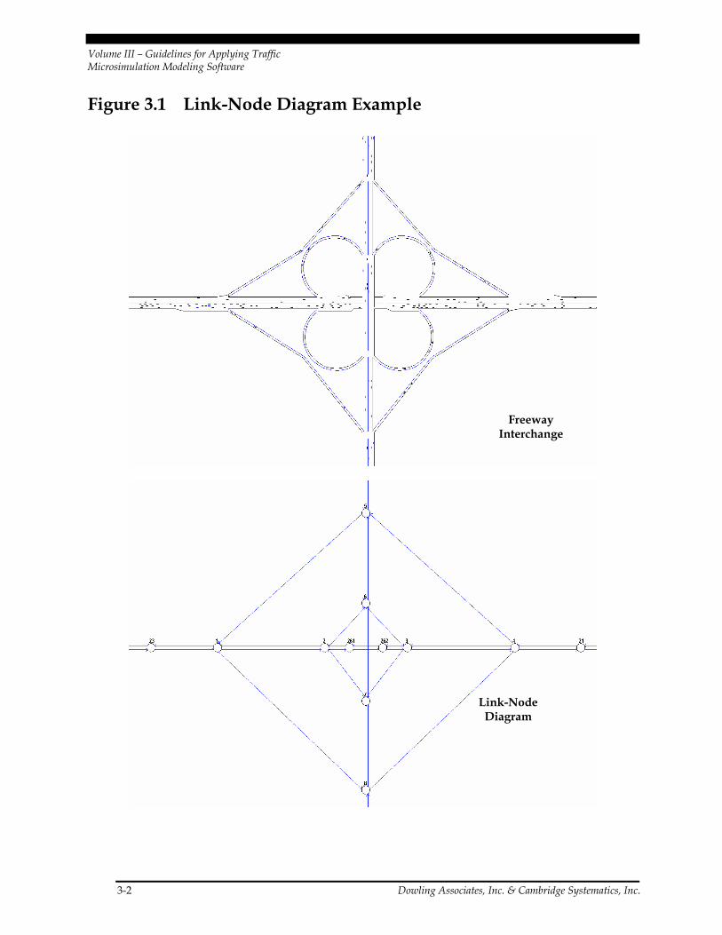
Volume III – Guidelines for Applying Traffic Microsimulation Modeling Software
3-2 Dowling Associates, Inc. & Cambridge Systematics, Inc.
Figure 3.1 Link-Node Diagram Example
Freeway Interchange
Link-Node Diagram

Volume III – Guidelines for Applying Traffic Microsimulation Modeling Software
Dowling Associates, Inc. &Cambridge Systematics, Inc. 3-3
Nodes are the intersection of two or more links. Nodes are usually placed in the model using X-Y coordinates and they can be at a place that represents an intersection or a loca-tion where there is a change in the link geometry. Some simulation software may also warrant the consideration of the Z coordinate. The nodes locations can be obtained from aerial photographs, maps, or physical measurements.
Links are one-directional segments of surface streets or freeways24. Links represent the length of the segment, and usually contain data on the geometric characteristics of the road or highway between nodes. Ideally, a link represents a roadway segment with uni-form geometry and traffic operations conditions25.
The analyst should consider establishing a node-numbering scheme to facilitate error checking and the aggregation of performance statistics for groups of links related to a spe-cific facility or facility type (see Table 3.1 for an example of a node numbering scheme designed to enable the rapid determination of the facility type in text output). Much of the output produced by microsimulation software is text, with results identified by the node numbers at the beginning and end points of each link. A node-numbering conven-tion can greatly facilitate the search for results in the massive text files commonly pro-duced by simulation software.26
If the link-node diagram was created off-line (using some other software beside the microsimulation software), then the information in the diagram needs to be entered (or imported) into the microsimulation software. The X-Y coordinates and identification numbers of the nodes (plus any feature points needed to represent link curvature) are entered. The nodes are then connected together to develop the link-node framework for the model.
24 Some software do not always use a link-node scheme, while other allows the analyst to code both
directions of travel with a single link. The two-way links coded by the user are then represented internally (inside the software) as two one-way links.
25 The analyst may find it desirable to split links for performance reporting purposes. For example, it may be desirable to report density separately for the 1,500-foot influence area on the freeway near a ramp merge or diverge. The analyst though should be cautious about the potential impact of split links on the capability of the software to accurately simulate vehicle behavior.
26 Some software provide analysis modules that assist the analyst in displaying and aggregating the results for specific groups of links. This feature reduces the strict necessity of adopting a node numbering convention, but a numbering convention can still result in significant labor savings when reviewing text output or importing text results into other software for analysis purposes.
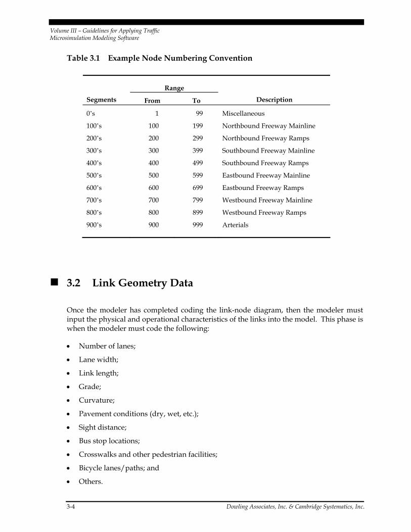
Volume III – Guidelines for Applying Traffic Microsimulation Modeling Software
3-4 Dowling Associates, Inc. & Cambridge Systematics, Inc.
Table 3.1 Example Node Numbering Convention
Range
Segments From To Description
0’s 1 99 Miscellaneous
100’s 100 199 Northbound Freeway Mainline
200’s 200 299 Northbound Freeway Ramps
300’s 300 399 Southbound Freeway Mainline
400’s 400 499 Southbound Freeway Ramps
500’s 500 599 Eastbound Freeway Mainline
600’s 600 699 Eastbound Freeway Ramps
700’s 700 799 Westbound Freeway Mainline
800’s 800 899 Westbound Freeway Ramps
900’s 900 999 Arterials
3.2 Link Geometry Data
Once the modeler has completed coding the link-node diagram, then the modeler must input the physical and operational characteristics of the links into the model. This phase is when the modeler must code the following:
• Number of lanes;
• Lane width;
• Link length;
• Grade;
• Curvature;
• Pavement conditions (dry, wet, etc.);
• Sight distance;
• Bus stop locations;
• Crosswalks and other pedestrian facilities;
• Bicycle lanes/paths; and
• Others.

Volume III – Guidelines for Applying Traffic Microsimulation Modeling Software
Dowling Associates, Inc. &Cambridge Systematics, Inc. 3-5
The specific data to be coded for the links will vary by the microsimulation software.
3.3 Traffic Control Data at Intersections and Junctions
Most microsimulation uses a time step simulation to describe traffic operations (which is usually one second or less). Vehicles are moved according to car-following logic, in response to traffic control devices and in response to other demands. Traffic control devices for microsimulation models will vary. Listed below are some examples:
• No control;
• Yield signs;
• Stop signs;
• Signals (pretimed, actuated, real-time traffic adaptive); and
• Ramp metering.
3.4 Traffic Operations and Management Data on Links
Traffic operations and management data for links consist of the following:
• Warning data (signs of incidents, lane drop, exit, etc.);
• Regulatory data (speed limit, variable speed limit, high-occupancy vehicle (HOV), HOT, detours, lane channelizations, lane use, etc.);
• Information (guidance) data (dynamic message signs and roadside beacons); and
• Surveillance detectors, type and location.
3.5 Traffic Demand Data
Traffic demands are defined as the number of vehicles and the percentage of vehicles of each type desiring to traverse the study area during the simulation time period. Further-more, it may be necessary to reflect the variation in demand throughout the simulation time period. In most software, the traffic entering into the network is usually defined by some parameter, and traffic leaving the network is usually computed based on parameters internal to the network such as turning movements and so on. The modeler must code the traffic volume by first starting from the external nodes (this is where the traffic is put into

Volume III – Guidelines for Applying Traffic Microsimulation Modeling Software
3-6 Dowling Associates, Inc. & Cambridge Systematics, Inc.
the model). Once all the entering traffic volumes at the external nodes are coded, the modeler will then go into the model and define the turning movements and any other parameter related to route choice. The key traffic demand data are:
• Entry volumes by vehicle type and turning fractions at all intersections or junctions (random walk simulators),
• O-D/path-specific and vehicle data (path-specific simulators),
• Bus operations (routes and headways/schedules), and
• Bicycle and pedestrian demand data.
3.6 Driver Behavior Data
Default values for driver behavior data are usually provided with the microsimulation software. Users may override the default values of any driver behavior parameters if valid observed data is available (e.g., desired free-flow speed, discharge headway, start-lost time at intersections, etc.). Driver behavior data includes:
• Driver’s aggressiveness (for minimum headway in car-following, gap acceptance for lane changing, response to yellow interval);
• Driver’s availability of (real-time) information; and
• Driver’s response to information (for pre-trip planning and or en-route switching).
3.7 Events/Scenarios Data
Events data includes:
• Blockages and incidents,
• Work zones, and
• Parking activities in curb lane.
This data is optional and will vary according to the specific application being developed by the analyst.

Volume III – Guidelines for Applying Traffic Microsimulation Modeling Software
Dowling Associates, Inc. &Cambridge Systematics, Inc. 3-7
3.8 Simulation Run Control Data
All simulation software contain run control parameters to enable the modeler to custom-ize the software operation for their specific modeling needs. These parameters will vary from software to software. They generally include:
• Length of simulation time;
• Selected MOEs or outputs (e.g., reports, animation files, or both);
• Resolution of simulation results (e.g., temporal and special resolution); and
• Other system parameters to run the model.
3.9 Coding Techniques for Complex Situations
Microsimulation software allows the modeler to develop a model to represent the “real-world” situation. However, not all possible real-world situations were necessarily con-templated when the software was originally written. This is when the modeler, with a good understanding of the operation of the software, can “extend” the software to simu-late conditions not originally incorporated in the microsimulation software. This should only be attempted, however, after a full appreciation of the tools, resources, and skills available. This is because new tools continue to become available which account for select “real-world” situations.
Provided below are some examples of how a basic microsimulation software can be extended to less standard situations, noting that calibration (discussed in Chapter 5) must also consider the situation:
1. A curb lane is heavily used for parking, loading, and unloading activities. As a result, this lane may be blocked “virtually” all the time. If the simulation software cannot correctly replicate the real situation, the modeler may consider removing this lane from the link.
2. There is a drawbridge in the real-world network but the software does not have an explicit “drawbridge,” model capability. If the boat traffic is very heavy and equiva-lent to “vehicular traffic”, the modeler may consider coding the drawbridge as an intersection with fixed-time signal control. If the boat traffic is irregular, the analyst might consider coding the drawbridge as a semi-actuated traffic signal controlled intersection. If boat traffic is rare then the drawbridge might be coded as a link with events that result in 100 percent capacity loss with a certain probability of occurrence during the analysis period.
3. Traffic regularly backs up on a freeway off-ramp, backing up onto the freeway. How-ever, instead of stopping on the freeway and blocking a lane, the queue forms on the

Volume III – Guidelines for Applying Traffic Microsimulation Modeling Software
3-8 Dowling Associates, Inc. & Cambridge Systematics, Inc.
shoulder of the freeway keeping the right-hand lane open. If this is the case in the study area, the modeler may artificially extend the off-ramp length to realistically model the traffic in the field.
3.10 Quality Assurance/Control Plan
Once the modeler is satisfied that the model is coded, then the modeler must vet the model for completeness. This could be a QA/QC process. Many of the models inputs are developed in a format that can be exported to a spreadsheet format. Therefore, the mod-eler can use this type of tool to aid in vetting the model for completeness and accuracy. The next chapter on error checking describes quality control tests in more detail.
3.11 Example Problem – Base Model Development
Continuing with the same example problem from the previous chapters, the task now is to code the base model.
The first step is to code the link-node diagram. How this is best done can be determined from the software user’s guide. Figure 3.2 shows the link-node diagram for the example problem.
The next steps are to input:
1. The link geometry data,
2. The intersection traffic control data,
3. The traffic operations and management data,
4. The traffic count data, and
5. The run control parameters.27
27 The software provided default values for driver behavior (aggressiveness, awareness, etc.) were
used in this example problem. They were considered to be sufficiently accurate for this analysis.

Volume III – Guidelines for Applying Traffic Microsimulation Modeling Software
Dowling Associates, Inc. &Cambridge Systematics, Inc. 3-9
Figure 3.2 Link-Node Diagram for Example Problem
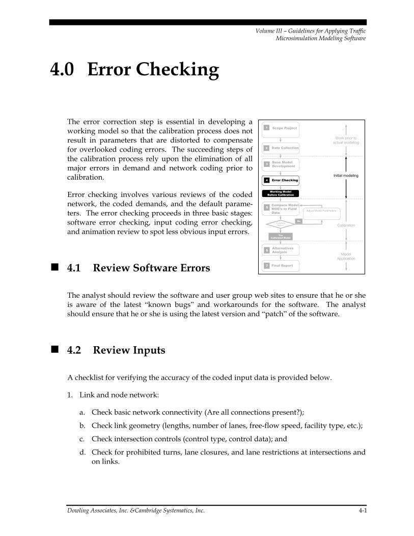
Volume III – Guidelines for Applying Traffic Microsimulation Modeling Software
Dowling Associates, Inc. &Cambridge Systematics, Inc. 4-1
4.0 Error Checking
The error correction step is essential in developing a working model so that the calibration process does not result in parameters that are distorted to compensate for overlooked coding errors. The succeeding steps of the calibration process rely upon the elimination of all major errors in demand and network coding prior to calibration.
Error checking involves various reviews of the coded network, the coded demands, and the default parame-ters. The error checking proceeds in three basic stages: software error checking, input coding error checking, and animation review to spot less obvious input errors.
4.1 Review Software Errors
The analyst should review the software and user group web sites to ensure that he or she is aware of the latest “known bugs” and workarounds for the software. The analyst should ensure that he or she is using the latest version and “patch” of the software.
4.2 Review Inputs
A checklist for verifying the accuracy of the coded input data is provided below.
1. Link and node network:
a. Check basic network connectivity (Are all connections present?);
b. Check link geometry (lengths, number of lanes, free-flow speed, facility type, etc.);
c. Check intersection controls (control type, control data); and
d. Check for prohibited turns, lane closures, and lane restrictions at intersections and on links.
Working ModelBefore Calibration
4
7
Error Checking
1 Scope Project
2 Data Collection
3 Base Model Development
Work prior toactual modeling
Initial modeling
YesCalibrated Model
5Compare ModelMOE’s to FieldData
Calibration
6 Alternatives Analysis
Adjust Model Parameters
Final Report
AcceptableMatch?
No
ModelApplication
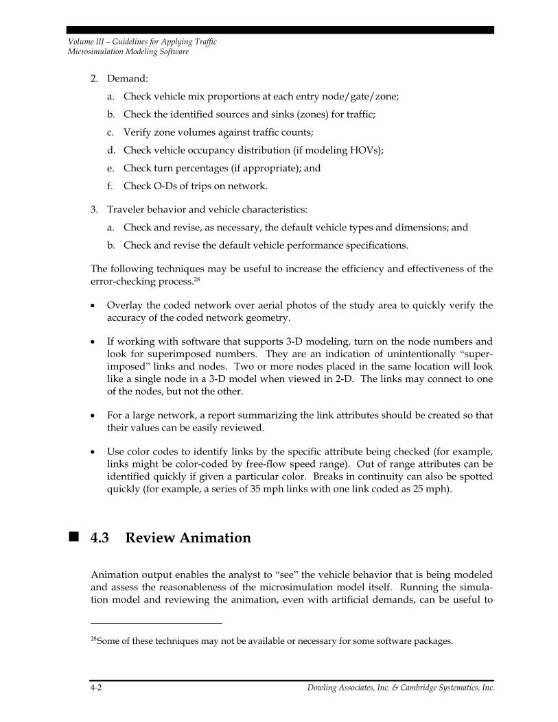
Volume III – Guidelines for Applying Traffic Microsimulation Modeling Software
4-2 Dowling Associates, Inc. & Cambridge Systematics, Inc.
2. Demand:
a. Check vehicle mix proportions at each entry node/gate/zone;
b. Check the identified sources and sinks (zones) for traffic;
c. Verify zone volumes against traffic counts;
d. Check vehicle occupancy distribution (if modeling HOVs);
e. Check turn percentages (if appropriate); and
f. Check O-Ds of trips on network.
3. Traveler behavior and vehicle characteristics:
a. Check and revise, as necessary, the default vehicle types and dimensions; and
b. Check and revise the default vehicle performance specifications.
The following techniques may be useful to increase the efficiency and effectiveness of the error-checking process.28
• Overlay the coded network over aerial photos of the study area to quickly verify the accuracy of the coded network geometry.
• If working with software that supports 3-D modeling, turn on the node numbers and look for superimposed numbers. They are an indication of unintentionally “super-imposed” links and nodes. Two or more nodes placed in the same location will look like a single node in a 3-D model when viewed in 2-D. The links may connect to one of the nodes, but not the other.
• For a large network, a report summarizing the link attributes should be created so that their values can be easily reviewed.
• Use color codes to identify links by the specific attribute being checked (for example, links might be color-coded by free-flow speed range). Out of range attributes can be identified quickly if given a particular color. Breaks in continuity can also be spotted quickly (for example, a series of 35 mph links with one link coded as 25 mph).
4.3 Review Animation
Animation output enables the analyst to “see” the vehicle behavior that is being modeled and assess the reasonableness of the microsimulation model itself. Running the simula-tion model and reviewing the animation, even with artificial demands, can be useful to
28 Some of these techniques may not be available or necessary for some software packages.
Volume III – Guidelines for Applying Traffic Microsimulation Modeling Software
Dowling Associates, Inc. &Cambridge Systematics, Inc. 4-3
identify input coding errors. The analyst inputs a very low level of demand and then fol-lows individual vehicles through the network. Aberrant vehicle behavior (such as unex-pected braking, or stops) is a quick indicator of possible coding errors.
A two-stage process can be followed in reviewing the animation output.
1. Run the animation at an extremely low demand level, so low that there is no conges-tion. The analyst should then trace single vehicles through the network and see where they unexpectedly slow down. These will usually be locations of minor network coding errors that disturb the movement of vehicles over the link or through the node. This test should be repeated for several different O-D zone pairs.
2. Once the extremely low demand level tests are completed, then run the simulation at 50 percent of existing demand level. At this level, demand is usually not yet high enough to cause congestion. If congestion appears, it may be the result of some more subtle coding errors that affect the distribution of vehicles across lanes or their head-ways. Check entry and exit link flows to verify that all demand is being correctly loaded and moved through the network.
The animation should be observed in close detail at key congestion points to determine if the animated vehicle behavior is realistic. If the observed vehicle behavior appears unre-alistic, the analyst should search through the following potential causes of the unrealistic animation in the order shown below:
1. Error in analyst expectations. The analyst should first verify in the field the correct vehicle behavior for the location and time period being simulated before deciding that the animation is showing unrealistic vehicle behavior. Many times, analyst expecta-tions of realistic vehicle behavior are not matched by actual behavior in the field.29 Field inspection may also reveal causes of vehicle behavior not apparent when coding the network from plans and aerial photos. These causes need to be coded into the model if the model is expected to produce realistic behavior.30
2. Analyst data coding errors. The analyst should next check for data coding errors that may be causing the simulation model to represent travel behavior incorrectly. Subtle data coding errors are the most frequent cause of unrealistic vehicle behavior in com-mercial microsimulation models that have already been subjected to extensive validation.
29 Analysts should not expect classic macroscopic traffic flow concepts to apply at the microscopic,
individual vehicle level. Macroscopic flow concepts, such as no variance in mean speed at low flow rates, do not apply to the behavior of an individual vehicle over the length of highway. An individual vehicle’s speed may vary over the length of the highway, and between vehicles, even at low flow rates. Macroscopic flow theory speaks of the average speed of all vehicles being relatively constant at low flow rates, not individuals.
30 A Traffic Management Center (TMC) with high density camera spacing will be very helpful in reviewing the working model. Many TMCs are now providing workstations for traffic analysis/ simulation staff.

Volume III – Guidelines for Applying Traffic Microsimulation Modeling Software
4-4 Dowling Associates, Inc. & Cambridge Systematics, Inc.
Subtle coding errors include apparently correctly coded inputs that are incorrect because of how they are used in the model to determine vehicle behavior.31
Comparing the model animation to the field design and operations cannot be overempha-sized. Some of the things to look for include:
• Overlooked data values needing refinement;
• Aberrant vehicle operations such as drivers using shoulders as a turning or travel lane, etc.;
• Previously unidentified points of major ingress or egress (these might be modeled as an intersecting street);
• Operations that the model cannot explicitly replicate (certain operations in certain tools/models), such as a two-way center turn lane (this might be modeled as an alter-nating short turn-bay);
• Unusual parking configurations such as median parking (this might be modeled operationally by reducing the free-flow speed to account for this “friction”);
• Average travel speeds may exceed posted or legal speeds (use the observed average speed in the calibration process);
• Turn-bays that cannot be fully utilized due to being blocked by through traffic; and
• In general, localized problems that can result in system-wide impacts.
4.4 Residual Errors
If the analyst has field verified his or her expectations of traffic performance and has exhausted all possible input errors, and the simulation still does not perform to the ana-lyst’s satisfaction, there are still a few possibilities. The desired performance may be beyond the capabilities of the software, or there may be a software error.
Software limitations can be identified through careful review of the software documenta-tion. If software limitations are a problem, then the analyst will have to “work around”
31 For example, it could be that the warning sign for an upcoming off-ramp is posted in the real-
world one-quarter mile before the off-ramp, but because the model uses warning signs to identify where people start positioning themselves for the exit ramps, the analyst may have to code the warning sign at a different location, the location where field observations indicate where the majority of drivers start positioning themselves for the off-ramp.

Volume III – Guidelines for Applying Traffic Microsimulation Modeling Software
Dowling Associates, Inc. &Cambridge Systematics, Inc. 4-5
the limitations by “tricking” or “forcing” the model to produce the desired performance32. If the limits are too great, the analyst might seek an alternate software package without the limitations. Advanced analysts can also write their own software interface with the microsimulation software (called application program interface (API)) to overcome the limitations and produce the desired performance.
Software errors can be tested by coding simple test problems (such as a single link or intersection) where the result (such as capacity or mean speed) can be computed manually and compared to the model. Software errors can only be resolved by working with the software developer.
4.5 Key Decision Point
The completion of error checking is a key decision point. The next task, model calibration, can be very time consuming. Before embarking upon this next task, the analyst should confirm that error checking is complete, specifically:
1. All input data are correct;
2. Values of all initial parameters and default parameters are reasonable; and
3. Animated results look fine based on “judgment” or “field inspection.”
Once the error checking is complete, the analyst has a working model (though it is still uncalibrated).
4.6 Example Problem – Error Checking
We continue with the same example problem from the previous chapters. The task now is to error check the coded base model.
Software. The latest version of the software was used. Review of the model documenta-tion and other material in the software and user groups’ web sites indicated that that there were no known problems or bugs related to the network under study and the scenarios to be simulated.
Review of input data and parameters. The coded input data were verified using the input files, the input data portion of the output files, static displays, and animation.
32 For example, a drawbridge that opens regularly might be coded as a traffic signal.
Volume III – Guidelines for Applying Traffic Microsimulation Modeling Software
4-6 Dowling Associates, Inc. & Cambridge Systematics, Inc.
First, the basic network connectivity was checked and its consistency with coded geome-try and turning restrictions. All identified errors found were corrected. For example, one link with exclusive left- and right-turn lanes (no through traffic) was coded as feeding a downstream through link.
Static network displays were used extensively to verify number of lanes, lane utilization, lane alignment (i.e., lane number that feeds the downstream through link), and location of lane drops. At this step, the consistency of link attributes was checked. For example, is the free-flow speed of 55 mph coded for all freeway links?
Next, the traffic demand data were checked. Input volumes at the network entrances were specified in four time slices. The input values were checked against the collected data.
Special attention was given to the traffic patterns at the interchange ramp terminals to avoid unrealistic movements. The software provisions (and options) were exercised to force the model not to assign movements to infeasible travel paths33.
The vehicle characteristics and performance data were reviewed.
The model displays and animation were used to verify the input data and operation of the traffic signals coded at each intersection. For fixed-time signals, the phasing and signal settings were checked (see Figure 4.1). For actuated signals, initial simulation were per-formed with reduced but balanced volumes to ensure that all phases are activated by the traffic demand. This was done because often inappropriate settings of phase flags cause signals “to malfunction” within the simulation and produce unreasonable results. This step also involves checking the detectors location and association with signal phases.
Review animation. Following the checking of the input data, the model was run using very low demand volumes to verify that the all vehicles travel the network without slow downs. This step uncovered minor errors to the links alignments that needed to be adjusted.
Next, the traffic demands were specified to about 50 percent of the actual volumes and the simulation model was rerun. Animation was used to verify that all demands are properly loaded in the network links and the traffic signals are properly operating. The link and system performance measures (travel time, delay) were also checked for reasonabless (i.e., they should reflect free-flow conditions.)
33 An example of this would be the limitation or coding to address freeway drivers who do or do
not make U-turn at an interchange (i.e., get off and then back on the freeway in the opposite direction).

Volume III – Guidelines for Applying Traffic Microsimulation Modeling Software
Dowling Associates, Inc. &Cambridge Systematics, Inc. 4-7
Figure 4.1 Checking Intersection Geometry, Phasing, and Detectors
Careful checking of the animation revealed subtle coding problems. For example, the coded distance of a warning sign (for exiting vehicles) or the distance from the start of the link to the lane drop point affects the proper simulation of driver behavior. These prob-lems were corrected.
Key decision point. The model, as revised throughout the error-checking process, was run with all the input data (actual demands) and the default model parameters. The out-put and animation were reviewed and discussed also with other agency staff that were familiar with the study area. The conclusion is that the model is working properly.

Volume III – Guidelines for Applying Traffic Microsimulation Modeling Software
Dowling Associates, Inc. &Cambridge Systematics, Inc. 5-1
5.0 Calibration of Microsimulation Models
Upon completion of the error-checking task, the analyst has a working model. But without calibration, the analyst has no assurance that the model will correctly predict traffic performance for the project.
Calibration is the adjustment of model parameters to improve the model’s ability to reproduce local driver behavior and traffic performance characteristics. Cali-bration is performed on various components of the overall model.
The importance of calibration cannot be over empha-sized. Recent tests of six different software packages found that calibration differences of 13 percent in the predicted freeway speeds for existing conditions increased to differences of 69 percent in the forecasted freeway speeds for future conditions34.
5.1 Objectives of Calibration
Calibration is necessary because no single model can be expected to be equally accurate for all possi-ble traffic conditions. Even the most detailed microsimulation model still contains only a portion of all of the variables that affect real-world traffic conditions. Since no single model can include the whole universe of variables, every model must be adapted to local conditions.
Every microsimulation software package comes complete with a set of user adjustable parameters for the purpose of calibrating the model to local conditions. The objective of
34 Bloomberg, L., M. Swenson, B. Haldors, Comparison of Simulation Models and the Highway Capacity
Manual, Preprint, Annual Meeting Transportation Research Board, Washington, D.C., 2003.
Working ModelBefore Calibration
4
7
Error Checking
1 Scope Project
2 Data Collection
3 Base Model Development
Work prior toactual modeling
Initial modeling
YesCalibrated Model
5Compare ModelMOE’s to FieldData
Calibration
6 Alternatives Analysis
Adjust Model Parameters
Final Report
AcceptableMatch?
No
ModelApplication
The objective of calibration is to improve the ability of the model to accurately reproduce local traffic conditions.

Volume III – Guidelines for Applying Traffic Microsimulation Modeling Software
5-2 Dowling Associates, Inc. & Cambridge Systematics, Inc.
calibration, therefore, is to find the set of parameter values for the model that best repro-duce local traffic conditions.
The software developers provide suggested default values for the model parameters for the convenience of the analyst. However, only under very rare circumstances will the model be able to produce accurate results for a specific area using only default parameter values. The analyst should always perform some calibration tests to ensure that the coded model accurately reproduces local traffic conditions and behavior.
The fundamental assumption of calibration is that the travel behavior models in the simulation model are essentially sound.35 There is no need to verify that they produce the correct delay, travel time, and density, when they are given the correct input parameters for a link. The only remaining task for the analyst is, therefore, to adjust the parameters so that the models correctly predict local traffic conditions.
5.2 Calibration Approach
Calibration involves the review and adjustment of potentially hundreds of model parameters, each of which impacts the simulation results in a manner that is often highly correlated with that of the others. The analyst can easily get trapped in a never-ending circular process fixing one problem only to find a new one pops up somewhere else. Therefore, it is essential to break the calibration process into a series of logical, sequential steps, a “strategy” for calibration.
In order to make calibration practical, the parameters must be divided into categories and each category dealt with separately. The “available” calibration parameters should be divided by the analyst into the following two basic categories:
1. Parameters that the analyst is certain about and does not wish to adjust, and
2. Parameters that the analyst is less certain about and willing to adjust.
The analyst should attempt to keep the set of adjustable parameters to as small a set as possible in order to minimize the effort required to calibrate them. However, the tradeoff is that more parameters allow the analyst more degrees of freedom to better fit the cali-brated model to the specific location.
The set of “adjustable” parameters is then further subdivided into those that directly impact capacity (such as mean headway) and those that directly impact route choice. The capacity adjustment parameters are calibrated first, the route choice adjustment parame-ters are then calibrated second. 35 The analyst determines the soundness of the simulation software when selecting it for use in the
study.

Volume III – Guidelines for Applying Traffic Microsimulation Modeling Software
Dowling Associates, Inc. &Cambridge Systematics, Inc. 5-3
Calibration strategy:
1. Calibrate capacity parameters,
2. Calibrate route choice parameters, and
3. Calibrate overall model performance.
Each set of adjustable parameters can be further subdivided into those that affect the simulation on a global basis and those that affect the simulation on a more localized basis. The global parameters are calibrated first. The “local” link-specific parameters are used after the global calibration to fine-tune the results.
The following three-step strategy is recommended for calibration:
1. Capacity calibration. An initial calibration is performed to identify the values for the capacity adjustment parameters that cause the model to best reproduce observed traffic capacities in the field. A global calibration is first performed, followed up by link-specific fine-tuning. The HCM can be used as an alternative source of capacity target values, if field measurements are infeasible.
2. Route choice calibration. If the microsimulation model includes parallel streets, then route choice will be important. In this case, a second calibration process is performed, but this time with the route choice parameters. A global calibration is first performed, followed by link-specific fine-tuning.
3. System performance calibration. Finally, the overall model estimates of system per-formance (travel times and queues) are compared to field measurements of travel times and queues. Fine-tuning adjustments are made to enable the model to better match the field measurements.
5.3 Step One: Calibration for Capacity
The capacity calibration step adjusts the global and link-specific “capacity-related” parameters in the simulation model to best replicate local field measurements of capacity. This is an important step because capacity has a significant effect on predicted system per-formance (delay and queues).36 The objective of this calibration step is to find a set of model parameters that cause the model to come as close as possible to matching field measurements of traffic capacity.
36 Historically, it has been the practice to calibrate microsimulation models to all the traffic counts in
the field. The majority of these counts will be at non-critical locations. The recommended strategy is to focus (at this point of the calibration process) only on the critical counts at the bottlenecks and get the model to reproduce these counts correctly. Once this is done, the rest of the counts are used later to check the route choice aspects of the model. All of this pre-supposes that the demands have been entered correctly and already have been checked against counts at the entry gates as part of the first step, error checking.

Volume III – Guidelines for Applying Traffic Microsimulation Modeling Software
5-4 Dowling Associates, Inc. & Cambridge Systematics, Inc.
Capacity calibration has two phases:
1. Global calibration, and
2. Link fine-tuning.
The capacity calibration step consists of two phases: 1) a global calibration phase, and 2) a fine-tuning phase. Global calibration is first performed to iden-tify the appropriate network-wide value of the capacity parameter(s) that best reproduces conditions in the field. Link-specific capacity parameters are then adjusted to fine tune the model so that it more precisely matches the field measured capacities at each and every bottleneck.37
The capacity calibration procedure is as follows:
1. Collect field measurements of capacity,
2. Obtain model estimates of capacity,
3. Select parameters to be calibrated,
4. Set calibration objective function,
5. Perform search for optimal parameter value, and
6. Fine-tune the calibration.
The following subsections explain this procedure in more detail.
5.3.1 Collect Field Measurements of Capacity
The identification of locations for field measurements of capacity will depend upon the existing traffic conditions within the study area.
For unsignalized facilities (freeways, rural highways, and rural roads), the analyst should identify locations where queues persist for at least 15 minutes and measure the flow rate at the point where the queue discharges. This observed flow rate is measured only while an upstream queue is present. It is summed across all lanes and converted to an equiva-lent hourly flow rate. This is the field-measured capacity of the facility at this point.
For signalized intersections, the analyst should identify the approach legs that frequently have queues of at least 10 vehicles per lane and measure the saturation flow rate per hour per lane using the procedures outlined in the appendix to the signalized intersection chapter of HCM. The capacity of the signalized intersection approach is then the satura-tion flow multiplied by the portion of green time in the signal cycle:
37 It is certainly possible to use link-specific parameters exclusively during the capacity calibration
step, but this eliminates the benefits of the global parameter adjustment. The global adjustment ensures the accuracy of the model-predicted capacities on all links (even those not currently congested). Adjustment of link-specific parameters ensures the model accuracy only for the specific link.

Volume III – Guidelines for Applying Traffic Microsimulation Modeling Software
Dowling Associates, Inc. &Cambridge Systematics, Inc. 5-5
If the model initially shows no congestion at the bottlenecks, the demand must be temporarily increased before calibration can proceed.
All “false” bottlenecks in the model must be cleared before calibration can proceed.
Cgsc =
Where:
c = capacity (veh/hr),
s = saturation flow (veh/hr/green),
g = effective green time, and
C = cycle length.
Higher saturation flows and lower start-up lost times result in higher capacities.
Several measurements of maximum flow rates should be made in the field and averaged. Procedures are provided in the appendix for estimating how many measurements are required to estimate capacity within a desired confidence interval (see Appendix B – Confidence Intervals). If capacity cannot be measured in the field, then the methods of the HCM can be used to estimate capacity. The HCM methods should not be considered a default technique, since the estimates are not as accurate as direct field measurements.
5.3.2 Obtain Model Estimates of Capacity
Microsimulation models do not output a number called “capacity.” Instead, they output the number of vehicles that pass a given point. So the analyst must manipulate the input demand as necessary to create a queue upstream of the target section to be calibrated so that the model will report the maximum possible flow rate through the bottleneck.
If the model does not initially show congestion at the same bottleneck locations as exist in the field, then the demands coded in the model are tempo-rarily increased to force the creation of congestion at those bottlenecks. These temporary increases must be removed later after the capacity calibration is complete, but before the route choice calibration step.
If the model initially shows congested bottlenecks at locations that do NOT exist in the field, it will be necessary to temporarily increase the capacity at those false bottlenecks (using temporary link-specific headway adjustments). These temporary adjustments are then removed during the fine-tuning phase.
For unsignalized facilities (freeways, rural highways, and rural roads), the simulated queue should persist for at least 15 minutes of simulated time, across all lanes and links feeding the target section. The simulated capacity is then the mean flow rate at the target section (measured at a detector placed in the target section and summed across all lanes)

Volume III – Guidelines for Applying Traffic Microsimulation Modeling Software
5-6 Dowling Associates, Inc. & Cambridge Systematics, Inc.
averaged over the 15-minute or longer period that the queue is present. The result is then divided by the number of lanes and converted to an hourly flow rate.
For signalized intersections, the coded demand should be increased as necessary to ensure the necessary queues of at least 10 vehicles at the start of green. A detector is placed in the model at the stopline to measure the discharge headways (on a per lane basis) of the first 10 vehicles crossing the detector in each lane38. The per-lane headways are averaged for each lane and then averaged across lanes. The result is then converted to an hourly flow rate per lane.
Just as the field measurements of capacity were repeated several times and the results averaged, the model runs should be repeated several times and the maximum flow rate at each location averaged across the runs. The minimum required number of runs to obtain a value of capacity within a desired confidence interval can be calculated using the proce-dures provided in Appendix B (Confidence Intervals).
5.3.3 Select Calibration Parameter(s)
Only the model parameters that directly affect capacity are calibrated at this time. Each microsimulation software package has its own set of parameters that affect capacity, depending upon the specific car-following and lane-changing logic implemented in the software. The analyst must review the software documentation and select one or two of these parameters for calibration.
The chapter does not intend to describe all the parameters for all the simulation models that are available. An illustrative list of capacity related parameters for freeways and sig-nalized arterials is given below:
Freeway facilities:
• Mean following headway,
• Driver reaction time,
• Critical gap for lane changing, and
• Minimum separation in stop and go conditions.
Signalized intersections:
• Start-up lost time,
• Queue discharge headway, and
• Gap acceptance for unprotected left turns.
38 The headways for the first three vehicles are discarded.

Volume III – Guidelines for Applying Traffic Microsimulation Modeling Software
Dowling Associates, Inc. &Cambridge Systematics, Inc. 5-7
Mean Headway is a good global parameter for calibrating capacity. It may have different names in different software.
For example, in CORSIM, the two parameters that most globally affect capacity are “headway factor by vehicle type” (Record Type 58) and “car following sensitivity factor” (Record Type 68). There are numerous other parameters in CORSIM that affect capacity, but they mostly apply only to specific conditions (for example, “acceptable gap in near-side cross traffic for vehicles at a stop sign” – Record Type 142).
For the fine-tuning phase in CORSIM, the link-specific capacity calibration parameter is “mean queue discharge headway,” which can be found on Record Type 11 for city streets, and on Record Type 20 for freeways (“link-specific car-following sensitivity multiplier”).
5.3.4 Set Calibration Objective Function
It is recommended that the analyst seek to minimize the mean square error (MSE) between the model estimates of maximum achievable flow rates and the field measure-ments of capacity. The MSE is the sum of the squared errors averaged over several model run repetitions. Each set of repetitions has a single set of model parameter values (p) with different random number seeds39 for each repetition within the set.40
Select a set of model parameters “p” so as to minimize:
∑ −=r
lltpr FMR
MSE 2)(1
Subject to:
maxminmmm ppp ≤≤ for all user-adjustable model parameters “pm”
39 Microsimulation models assign driver–vehicle characteristics from statistical distributions using
random numbers. The sequence of random numbers generated depends on the initial value of the random number (random number seed). Changing the random number seed produces a different sequence of random numbers, which, in turn, produces different values of driver-vehicle characteristics.
40 Some researchers have calibrated models using the percent mean square error in order to avoid the unintended weighting effect when combining different measures of performance (such as volumes and travel time) into one measure of error. The percent MSE divides each square error by the field-measured value. The effect of using percent MSE is to place greater weight on large percentage errors rather than on large numerical errors. The simple MSE is recommended for calibration, because it is most sensitive to large volume errors.
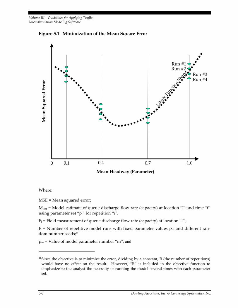
Volume III – Guidelines for Applying Traffic Microsimulation Modeling Software
5-8 Dowling Associates, Inc. & Cambridge Systematics, Inc.
Figure 5.1 Minimization of the Mean Square Error
0 0.4 0.7
Mea
n Sq
uare
d Er
ror
Mean Headway (Parameter)
0.1 1.0
Run #1Run #2
Run #3Run #4
Likely
Func
tion S
hape
Where:
MSE = Mean squared error;
Mltpr = Model estimate of queue discharge flow rate (capacity) at location “l” and time “t” using parameter set “p”, for repetition “r”;
Fl = Field measurement of queue discharge flow rate (capacity) at location “l”;
R = Number of repetitive model runs with fixed parameter values pm and different ran-dom number seeds;41
pm = Value of model parameter number “m”; and
41 Since the objective is to minimize the error, dividing by a constant, R (the number of repetitions)
would have no effect on the result. However, “R” is included in the objective function to emphasize to the analyst the necessity of running the model several times with each parameter set.
Volume III – Guidelines for Applying Traffic Microsimulation Modeling Software
Dowling Associates, Inc. &Cambridge Systematics, Inc. 5-9
Link-specific adjustment factors are often still necessary after global calibration, but they should be used sparingly.
pminm, pmaxm = User specified limits to the allowable range of parameter values (pm). Limits are necessary to avoid solutions that violate laws of physics, vehicle performance limits, and driver behavior extremes.
5.3.5 Perform Search for Optimal Parameter Value
The analyst must now find the capacity adjustment factor(s), “p”, that minimizes the MSE between the model and the field measurements of capacity. The calibration problem is a “non-linear”, “least-squares” optimization problem.
Since simulation models are complex models, it is not usually possible to formulate the models as a closed form equation for which traditional calculus techniques can be applied to find a minimum value solution. It is necessary to use some sort of search algorithm that relies upon multiple operations of the simulation model, plotting of the output results as points, and searching between these points for the optimal solution. Search algorithms are required to find the optimal solution to the calibration problem.
There are many software packages available for identifying the optimal combination of calibration parameters for minimizing the squared error between the field observations and the simulation model. The Optimization Technology Center Web Site of the Argonne National Laboratory and Northwestern University lists several software packages for “non-linear least squares” parameter estimation. See the following:
http://www-fp.mcs.anl.gov/otc/Guide/SoftwareGuide/Categories/nonlinleastsq.html
Appendix D describes a few simple search algorithms that can be applied manually or with the aid of spreadsheets. The exhibit below illustrates how a single parameter search (m = 1) might look using one of these simple search algorithms for the number of model runs (R) set to 4.
5.3.6 Fine-Tune the Calibration
Once the optimal global capacity calibration parameter values have been identified, there will still be some locations where model performance deviates a great deal from field con-ditions. The next phase is, therefore, to fine-tune the predicted capacity to match the location-specific measurements of capacity as closely as possible.
Link-specific capacity adjustments account for the roadside factors that affect capacity but are not typically coded in the microsimulation network input data set (such as presence of on-street parking, numerous driveways, or narrow shoulders). Most simulation software packages have link-specific capacity (or headway) adjustment factors that apply only to the subject link. These capacity adjustment factors are used to fine-tune the model calibration. Link-specific adjustment factors should be used sparingly since

Volume III – Guidelines for Applying Traffic Microsimulation Modeling Software
5-10 Dowling Associates, Inc. & Cambridge Systematics, Inc.
they are not behavior based. They are fixed adjustments that will be carried through all future runs of the simulation model.
5.4 Step 2: Route Choice Calibration
Once the analyst is satisfied that the model reproduces as closely as possible field meas-ured capacities, the next step is then to calibrate the route choice parameters in the model to better match observed flows. The temporary demand adjustments used in the previous capacity calibration step are reversed. The model predicted volumes are then compared to field counts and the analyst adjusts the route choice algorithm parameters until the best volume fit is achieved.42
If the model network consists of only a single facility, then no route choice calibration is possible or needed. This step is skipped.43 This step is also skipped for microsimulation software that does not have route choice capabilities.
Route choice calibration proceeds in two phases: 1) global calibration and 2) link-specific fine-tuning.
5.5.1 Global Calibration
Global calibration of route choice consists of the application of a route choice algorithm and associated parameters44. The specific parameters vary by algorithm and software package, but usually involve weights placed on the actual cost and travel time of each route. Additional parameters may relate to the familiarity of the driver with each route and the amount of error in the driver’s perception of the cost and time for each route. The analyst must review the software documentation and select one or two of these parame-ters for calibration. Global calibration then proceeds through the same process as was used to calibrate capacity. The MSE between the field counts and the model volume esti-mates is minimized using one of the available non-linear optimization techniques.
42 The specific route-choice algorithm parameters will vary by software package. They generally
relate to the driver’s awareness of, perception and sensitivity to travel time, delay, and cost of alternate routes.
43 For a single facility network, if there are still some remaining volume errors after the capacity calibration step, then the input demands should be error checked.
44 Some software packages allow to select the algorithm and its associated parameters.
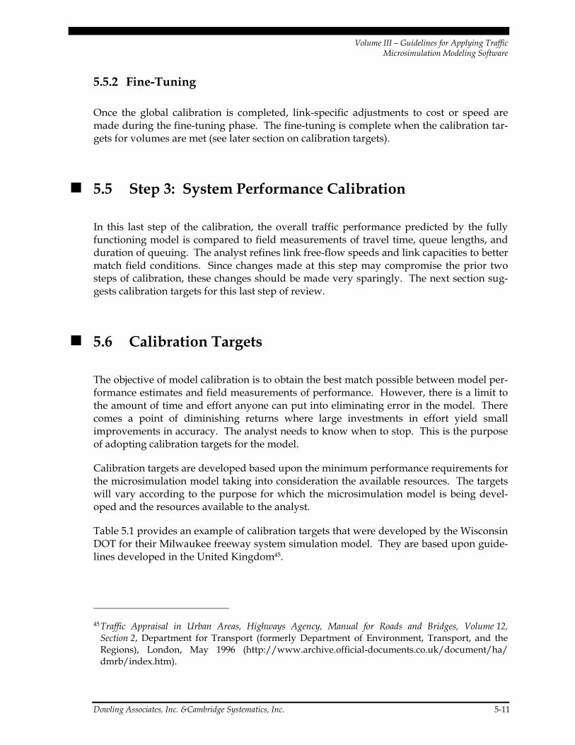
Volume III – Guidelines for Applying Traffic Microsimulation Modeling Software
Dowling Associates, Inc. &Cambridge Systematics, Inc. 5-11
5.5.2 Fine-Tuning
Once the global calibration is completed, link-specific adjustments to cost or speed are made during the fine-tuning phase. The fine-tuning is complete when the calibration tar-gets for volumes are met (see later section on calibration targets).
5.5 Step 3: System Performance Calibration
In this last step of the calibration, the overall traffic performance predicted by the fully functioning model is compared to field measurements of travel time, queue lengths, and duration of queuing. The analyst refines link free-flow speeds and link capacities to better match field conditions. Since changes made at this step may compromise the prior two steps of calibration, these changes should be made very sparingly. The next section sug-gests calibration targets for this last step of review.
5.6 Calibration Targets
The objective of model calibration is to obtain the best match possible between model per-formance estimates and field measurements of performance. However, there is a limit to the amount of time and effort anyone can put into eliminating error in the model. There comes a point of diminishing returns where large investments in effort yield small improvements in accuracy. The analyst needs to know when to stop. This is the purpose of adopting calibration targets for the model.
Calibration targets are developed based upon the minimum performance requirements for the microsimulation model taking into consideration the available resources. The targets will vary according to the purpose for which the microsimulation model is being devel-oped and the resources available to the analyst.
Table 5.1 provides an example of calibration targets that were developed by the Wisconsin DOT for their Milwaukee freeway system simulation model. They are based upon guide-lines developed in the United Kingdom45.
45 Traffic Appraisal in Urban Areas, Highways Agency, Manual for Roads and Bridges, Volume 12,
Section 2, Department for Transport (formerly Department of Environment, Transport, and the Regions), London, May 1996 (http://www.archive.official-documents.co.uk/document/ha/ dmrb/index.htm).

Volume III – Guidelines for Applying Traffic Microsimulation Modeling Software
5-12 Dowling Associates, Inc. & Cambridge Systematics, Inc.
Table 5.1 Wisconsin DOT Freeway Model Calibration Criteria
Criteria and Measures Calibration Acceptance Targets
Hourly Flows, Model Versus Observed
Individual Link Flows Within 15%, for 700 vph < Flow < 2,700 vph >85% of cases Within 100 vph, for Flow < 700 vph >85% of cases Within 400 vph, for Flow > 2,700 vph >85% of cases
Sum of all Link Flows Within 5% of sum of all link counts
GEH Statistic < 5 for Individual Link Flows* >85% of cases
GEH statistic for Sum of all Link Flows GEH < 4 for sum of all link counts
Travel Times, Model Versus Observed
Journey times network Within 15% (or one minute, if higher) >85% of cases
Visual Audits
Individual link speeds Visually acceptable speed-flow relationship To analyst’s satisfaction
Bottlenecks Visually acceptable queuing To analyst’s satisfaction
*The GEH statistic is computed as follows:
( )2/)(
2
VEVEGEH
+−
=
Where: E = model estimated volume and V = field count. Source: Freeway System Operational Assessment, Technical Report I-33, Paramics Calibration and
Validation Guidelines, Draft, Wisconsin DOT, District 2, June 2002.
Another example of suggested calibration targets is included in MnDOT’s Advanced CORSIM Training Manual.46
46 Minnesota DOT, Advanced CORSIM Training Manual, prepared by Short, Elliott, Hendrickson,
Inc., 2002.

Volume III – Guidelines for Applying Traffic Microsimulation Modeling Software
Dowling Associates, Inc. &Cambridge Systematics, Inc. 5-13
5.7 Example Problem – Model Calibration The same example problem from the previous chapters is continued. The task now is to calibrate the model.
A review of the results produced by the working model at the end of the model develop-ment task indicates that there are discrepancies between the observed and simulated traf-fic performance. The purpose of the calibration process is to adjust the model parameters to better match field conditions.
Calibration for Capacity – Step 1: Global Calibration
Field data on capacity. The network under study is not congested. Therefore, field meas-urements of the capacity values on the freeway links and saturation flows at the traffic signals on the arterials cannot be obtained.
Two potential future bottleneck locations were selected on the study area network. The capacities for these potential bottleneck locations were estimated using the HCM 2000 procedures. The estimated value for the saturation flow for protected movements at sig-nalized intersections was 1,800 vehicles per hour of green per lane (vphgpl), and the capacity of freeway links was found to be 2,100 vphgpl.
Model estimates of capacity. The model estimates of capacity can be obtained from detector measurements or from the throughput values reported at the end of the simula-tion run. However, it is necessary to have upstream queues in order for the throughput values to represent capacity.
Due to the lack of existing congestion, the existing volumes on the network links had to be artificially increased to trigger congestion upstream of the bottleneck locations (the model throughput volumes at these bottleneck locations would then be the model estimated capacities).
Select calibration parameters. The global parameter calibration was performed using the following parameters:
• Mean queue discharge headway at traffic signals. The default value for this parameter in the model is 1.8 sec/veh (which is equivalent to a saturation flow of 2,000 vphgpl under ideal conditions). The queue discharge headway per vehicle type is randomly assigned by the model depending on the driver’s aggressiveness factor.
• Mean headway (or car-following sensitivity factor) for the freeway links. This repre-sents the minimum distance that a driver is willing to follow vehicles. The values of the headway (or sensitivity factors) depend again on the driver aggressiveness. Lower values would cause higher throughput.
Set calibration objective function. The criterion chosen to determine the optimal parameter value was the minimization of the MSE between the model estimates of satura-tion flow/capacity and the “field” estimates.
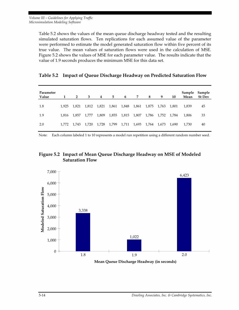
Volume III – Guidelines for Applying Traffic Microsimulation Modeling Software
5-14 Dowling Associates, Inc. & Cambridge Systematics, Inc.
Table 5.2 shows the values of the mean queue discharge headway tested and the resulting simulated saturation flows. Ten replications for each assumed value of the parameter were performed to estimate the model generated saturation flow within five percent of its true value. The mean values of saturation flows were used in the calculation of MSE. Figure 5.2 shows the values of MSE for each parameter value. The results indicate that the value of 1.9 seconds produces the minimum MSE for this data set.
Table 5.2 Impact of Queue Discharge Headway on Predicted Saturation Flow
Parameter Value 1 2 3 4 5 6 7 8 9 10
Sample Mean
Sample St Dev
1.8 1,925 1,821 1,812 1,821 1,861 1,848 1,861 1,875 1,763 1,801 1,839 45
1.9 1,816 1,857 1,777 1,809 1,855 1,815 1,807 1,786 1,752 1,784 1,806 33
2.0 1,772 1,743 1,720 1,728 1,799 1,711 1,693 1,764 1,673 1,690 1,730 40
Note: Each column labeled 1 to 10 represents a model run repetition using a different random number seed.
Figure 5.2 Impact of Mean Queue Discharge Headway on MSE of Modeled Saturation Flow
3,338
1,022
6,423
2.01.91.80
1,000
2,000
3,000
4,000
5,000
6,000
7,000
Mean Queue Discharge Headway (in seconds)
Mod
eled
Sat
urat
ion
Flow
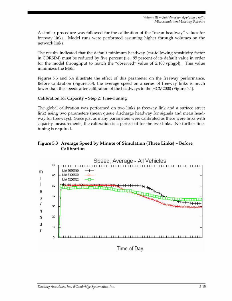
Volume III – Guidelines for Applying Traffic Microsimulation Modeling Software
Dowling Associates, Inc. &Cambridge Systematics, Inc. 5-15
A similar procedure was followed for the calibration of the “mean headway” values for freeway links. Model runs were performed assuming higher through volumes on the network links.
The results indicated that the default minimum headway (car-following sensitivity factor in CORSIM) must be reduced by five percent (i.e., 95 percent of its default value in order for the model throughput to match the “observed” value of 2,100 vphgpl). This value minimizes the MSE.
Figures 5.3 and 5.4 illustrate the effect of this parameter on the freeway performance. Before calibration (Figure 5.3), the average speed on a series of freeway links is much lower than the speeds after calibration of the headways to the HCM2000 (Figure 5.4).
Calibration for Capacity – Step 2: Fine-Tuning
The global calibration was performed on two links (a freeway link and a surface street link) using two parameters (mean queue discharge headway for signals and mean head-way for freeways). Since just as many parameters were calibrated as there were links with capacity measurements, the calibration is a perfect fit for the two links. No further fine-tuning is required.
Figure 5.3 Average Speed by Minute of Simulation (Three Links) – Before Calibration
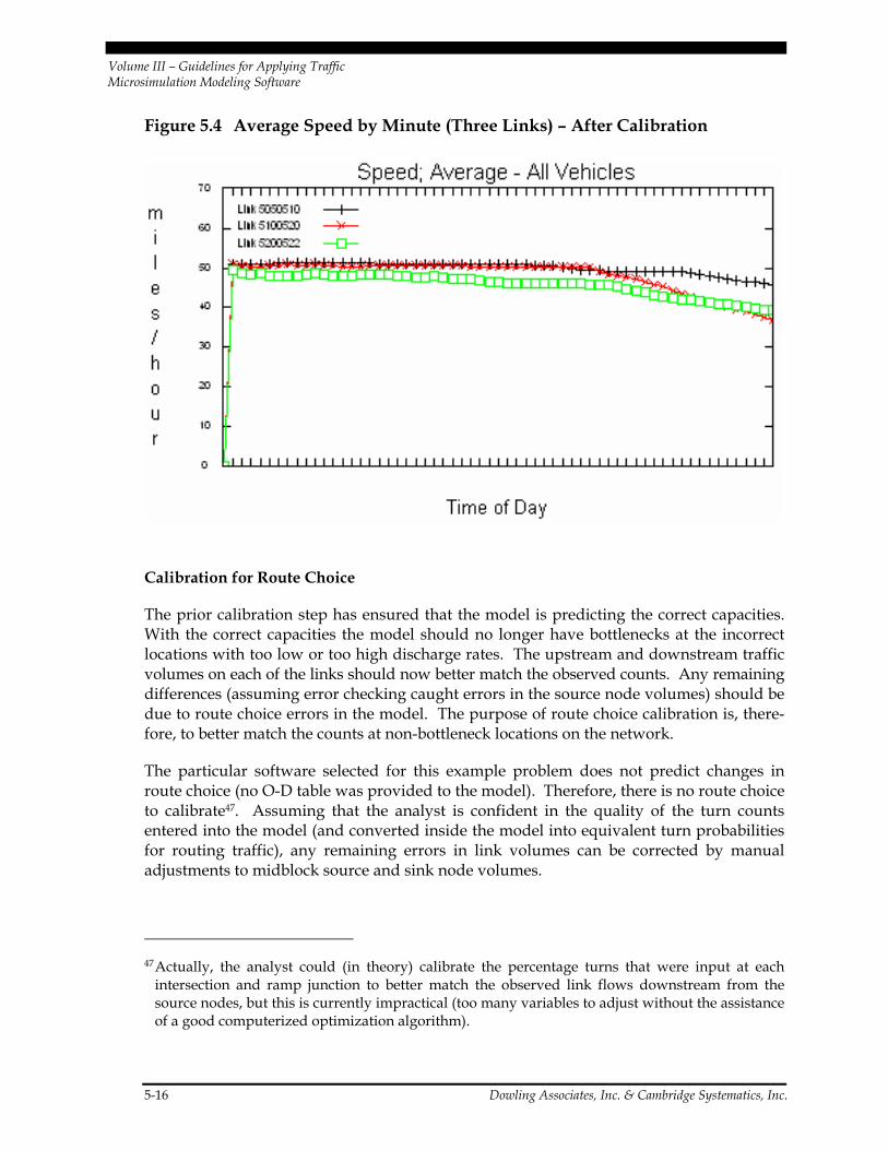
Volume III – Guidelines for Applying Traffic Microsimulation Modeling Software
5-16 Dowling Associates, Inc. & Cambridge Systematics, Inc.
Figure 5.4 Average Speed by Minute (Three Links) – After Calibration
Calibration for Route Choice
The prior calibration step has ensured that the model is predicting the correct capacities. With the correct capacities the model should no longer have bottlenecks at the incorrect locations with too low or too high discharge rates. The upstream and downstream traffic volumes on each of the links should now better match the observed counts. Any remaining differences (assuming error checking caught errors in the source node volumes) should be due to route choice errors in the model. The purpose of route choice calibration is, there-fore, to better match the counts at non-bottleneck locations on the network.
The particular software selected for this example problem does not predict changes in route choice (no O-D table was provided to the model). Therefore, there is no route choice to calibrate47. Assuming that the analyst is confident in the quality of the turn counts entered into the model (and converted inside the model into equivalent turn probabilities for routing traffic), any remaining errors in link volumes can be corrected by manual adjustments to midblock source and sink node volumes.
47 Actually, the analyst could (in theory) calibrate the percentage turns that were input at each
intersection and ramp junction to better match the observed link flows downstream from the source nodes, but this is currently impractical (too many variables to adjust without the assistance of a good computerized optimization algorithm).
Volume III – Guidelines for Applying Traffic Microsimulation Modeling Software
Dowling Associates, Inc. &Cambridge Systematics, Inc. 5-17
In this example problem, the freeway counts, ramp counts, and intersection counts were all adjusted at the data preparation stage to produce an internally consistent set of vol-umes for every link and node. There are no unaccounted for increases or decreases in volumes between nodes. Thus, no midblock source/sink nodes were required. The model predicted link volumes based on the source node volumes and the intersection turn percentages are consistent with the link counts (within the range of variation expected due to the random components of the simulation model).
System Performance Calibration
Once calibration is completed to the analyst’s satisfaction, the next step is to calibrate the overall performance of the model.
We compared the model predictions with the field data on speeds, travel times, and delays on the freeways and arterials.
Based on this comparison the free-flow speed distribution for the freeway was adjusted, so the model generated free-flow speeds are within a more narrow range than the default distribution. This reflects commute traffic behavior.
No other adjustments were made to the model parameters.
Ten repetitions of the calibrated data set were performed and the link outputs were proc-essed to produce performance measures to be compared with the field data.
The comparison is shown in Table 5.3. The simulated values represent the mean value of the MOEs based on the 10 model runs for the third time slice of the simulated peak hour.
Not shown here are comparisons with field measurement of delay, because it was unclear how the field data on delay were collected. In general, users must be cautious when they compare field versus simulated delays, because the delay is typically defined differently in most software packages than the approaches commonly used for field measurements.
The results indicate that the model satisfies the criteria for calibration (shown in Table 5.1).

Volume III – Guidelines for Applying Traffic Microsimulation Modeling Software
5-18 Dowling Associates, Inc. & Cambridge Systematics, Inc.
Table 5.3 System Performance Results for Example Problem
Travel Time (minutes) Speed (mph) Density (vehicle/mile/lane)
Freeway Segment Field Sim. Diff. Abs. %
Diff Field Sim. Diff. Abs. %
Diff Field Sim. Diff. Abs. %
Diff EB west of Wisconsin off 1.44 1.47 0.03 2.3% 53.5 52.42 -1.04 1.95% 38.1 36.4 -1.64 4.3% EB Wisconsin off to on 0.22 0.22 -0.01 2.4% 53.4 51.84 -1.56 2.93% 38.9 33.0 -5.94 15.3% EB Wisconsin onto Milwaukee off
1.00 0.95 -0.05 5.0% 48.1 51.29 3.18 6.61% 38.6 34.4 -4.23 11.0%
EB Milwaukee off to on 0.22 0.22 0.00 0.1% 55.0 52.24 -2.76 5.01% 30.3 31.4 1.13 3.7% EB east of Milwaukee on 1.12 1.15 0.04 3.4% 53.8 51.96 -1.83 3.40% 34.0 33.9 -0.14 0.4% WB east of Milwaukee off 1.11 1.13 0.02 2.1% 54.3 53.44 -0.85 1.57% 29.1 28.8 -0.25 0.9% WB Milwaukee off to on 0.22 0.22 0.00 1.0% 55.0 52.65 -2.35 4.26% 26.5 27.1 0.59 2.2% WB Milwaukee on to Wisconsin off
0.96 0.94 -0.02 2.4% 50.1 51.94 1.87 3.73% 30.4 31.0 0.61 2.0%
WB Wisconsin off to on 0.22 0.22 0.00 0.8% 55.0 52.46 -2.54 4.61% 28.5 29.6 1.09 3.8% WB west of Wisconsin on 1.42 1.48 0.06 4.0% 54.2 52.10 -2.09 3.85% 32.1 32.9 0.78 2.4% Average 2.4% 3.79% 4.6%
Travel Time (minutes)
Arterial Segment Field Sim. Diff. Abs. %
Diff SB Milwaukee between ramps
0.44 0.43 -0.01 3.0%
NB Milwaukee between ramps
0.47 0.48 0.01 3.1%
SB Wisconsin between ramps 0.57 0.58 0.01 2.4% NB Wisconsin between ramps
0.74 0.66 -0.08 11.0%
Average 4.9%
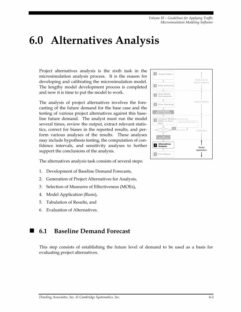
Volume III – Guidelines for Applying Traffic Microsimulation Modeling Software
Dowling Associates, Inc. & Cambridge Systematics, Inc. 6-1
6.0 Alternatives Analysis
Project alternatives analysis is the sixth task in the microsimulation analysis process. It is the reason for developing and calibrating the microsimulation model. The lengthy model development process is completed and now it is time to put the model to work.
The analysis of project alternatives involves the fore-casting of the future demand for the base case and the testing of various project alternatives against this base-line future demand. The analyst must run the model several times, review the output, extract relevant statis-tics, correct for biases in the reported results, and per-form various analyses of the results. These analyses may include hypothesis testing, the computation of con-fidence intervals, and sensitivity analyses to further support the conclusions of the analysis.
The alternatives analysis task consists of several steps:
1. Development of Baseline Demand Forecasts,
2. Generation of Project Alternatives for Analysis,
3. Selection of Measures of Effectiveness (MOEs),
4. Model Application (Runs),
5. Tabulation of Results, and
6. Evaluation of Alternatives.
6.1 Baseline Demand Forecast
This step consists of establishing the future level of demand to be used as a basis for evaluating project alternatives.
Working ModelBefore Calibration
4
7
Error Checking
1 Scope Project
2 Data Collection
3 Base Model Development
Work prior toactual modeling
Initial modeling
YesCalibrated Model
5Compare ModelMOE’s to FieldData
Calibration
6 Alternatives Analysis
Adjust Model Parameters
Final Report
AcceptableMatch?
No
ModelApplication

Volume III – Guidelines for Applying Traffic Microsimulation Modeling Software
6-2 Dowling Associates, Inc. & Cambridge Systematics, Inc.
6.1.1 Demand Forecasting
Forecasts of future travel demand are best obtained from a travel demand model. These models require a great deal of effort and time to develop and calibrate. If one does not already exist, then the analyst may seek to develop demand forecasts based on historic growth rates. A “trend-line” forecast might be made assuming that the recent percentage growth rate of traffic will continue in the future. These trend-line forecasts though are most reliable for relatively short periods (five years or less). They do not take into account the potential of future capacity constraints to restrict the growth of future demand. Addi-tional information and background regarding the development of traffic data for use in highway planning and design may be found in NCHRP Report 255, Highway Traffic Data for Urbanized Area Project Planning and Design.
6.1.2 Constraining Demand to Capacity
Regardless of which method is used to estimate future demand (regional model or trend line), care must be taken to ensure that the forecasts are a reasonable estimate of the actual amount of traffic that can arrive within the analysis period at the study area. Regional model forecasts are usually not well constrained to the system capacity, and trend-line forecasts are totally unconstrained. Appendix F provides a method for constraining future demands to the physical ability of the transportation system to deliver the traffic to the microsimulation model study area.
6.1.3 Allowance for Uncertainty in Demand Forecasts
All forecasts are subject to uncertainty. It is risky to design a road facility to a precise future condition, given the uncertainties in the forecasts. There are uncertainties in both the likely growth in demand and the available capacity that might be present in the future. Slight changes in the timing or design of planned or proposed capacity improvements outside of the study area can significantly change the amount of traffic delivered to the study area during the analysis period. Changes in future vehicle mix and peaking can easily affect capacity by 10 percent. Similarly, changes in economic development and public agency approvals of new development can significantly change the amount of future demand. Thus, it is good practice to explicitly plan for a certain amount of uncer-tainty in the analysis. This level of uncertainty is the purpose of sensitivity testing (explained in a separate section below).
6.2 Generation of Alternatives
In this step, the analyst generates improvement alternatives based upon direction from decision-makers and through project meetings. They will likely reflect operational strategies

Volume III – Guidelines for Applying Traffic Microsimulation Modeling Software
Dowling Associates, Inc. & Cambridge Systematics, Inc. 6-3
When reviewing model output, the analyst should look at a few key systemwide performance measures plus “hot spots” (indicators of localized breakdowns in the system).
and/or geometric improvements to address the problems identified based on the baseline demand forecasts. The specifics of alternatives generation are beyond the scope of this guide. Briefly, they consist of:
1. Performing a microsimulation analysis48 of the baseline demand forecast in order to identify the deficiencies,49 and
2. Identifying alternative improvements that solve one or more of the identified problems.50
6.3 Selection of MOEs
Measures of effectiveness are the system perform-ance statistics that best characterize the degree to which a particular alternative meets the project objectives (which were determined in the Project Scope Task). Thus, the appropriate MOEs are determined by the project objectives and agency performance standards, rather than what is produced by the model. This section, how-ever, discusses what outputs are typically produced by microsimulation software so that the analyst can appreciate what outputs might be available for constructing the desired MOEs.
Microsimulation, by its very nature, can bury the analyst in detailed, microscopic output. The key is to focus on a few key indicators of system performance and localized break-downs in the system (locations where queues are interfering with system operation).
48 A sketch-planning analysis using HCM techniques can be performed, if it is desired to identify
conceptual project alternatives prior to the development of a calibrated simulation model. The calibrated simulation model can then be used to refine the conceptual plans.
49 Deficiencies are identified by comparing the measured performance against the project objectives and agency performance standards identified in Task 1, Project Scope.
50 In support of the purpose and scope of the project, this identification of alternatives must take into consideration the range of demand conditions, weather conditions, incidents, and operational management strategies. Additional information and background may be found in the following documents: 1. Bunch, J., Hatcher, S., Larkin, J., Nelson, G., Proper, A., Roberts, D., Shah, V., and Wunderlich,
K., Incorporating ITS into Corridor Planning: Seattle Case Study, August 1999, EDL#11303. 2. Wunderlich, K. , Incorporating ITS into Planning Analyses: Summary of Key Findings from a
Seattle 2020 Case Study, FHWA-OP-02-031, May 2002, EDL#13605.

Volume III – Guidelines for Applying Traffic Microsimulation Modeling Software
6-4 Dowling Associates, Inc. & Cambridge Systematics, Inc.
6.3.1 Candidate MOEs for Overall System Performance
As explained above, the selection of MOEs should be driven by the project objectives and the agency performance standards; however, many MOEs of overall system performance can be computed directly or indirectly from the following three basic system performance measures:
1. Vehicle-miles traveled (VMT) or vehicle-kilometers traveled,
2. Vehicle-hours traveled (VHT), and
3. Mean system speed.
These three basic performance measures can also be supplemented with other model out-puts depending upon the objectives of the analysis. For example, total system delay is a useful overall system performance measure, when comparing the congestion relieving effectiveness of various alternatives. The number of stops is a useful indicator for signal coordination studies.
6.3.2 Candidate MOEs for Localized Problems
In addition to evaluating overall system performance, the analyst should also be evaluating if and where there are localized system breakdowns (hot spots). A hot spot may be indi-cated by a persistent short queue that lasts too long, a signal phase failure (green time fails to clear all waiting vehicles), or a blocked link (a queue that backs up into an upstream intersection).
A blocked link is the most significant indicator of localized breakdowns. A queue of vehi-cles that fills a link and blocks an upstream intersection can have significant performance impacts for the system. A link queue overflow report can be developed to identify the links and times during the simulation period when the computed queue of vehicles equaled (and, therefore, probably actually exceeded) the storage capacity of the link51.
Signal phase failures, where the provided green time is insufficient to clear the queue, indicate potential operations problems if the queues continue to build over several cycles. The analyst should develop a signal phase failure report to indicate when and where sig-nal green times are not sufficient to clear out all of the waiting queues of vehicles each cycle.
At the finest level of detail, the analyst may wish to develop a report of the presence of persistent queues of a minimum length. This hot spot report would identify persistent queues on a lane-by-lane basis of a minimum number of vehicles that persists for a minimum
51 This report will be less useful if the analyst has split long sections of roadway into arbitrary short
links for other reporting purposes. The result may be many “false alarms” of “blocked links” that do not actually obstruct an upstream intersection.
Volume III – Guidelines for Applying Traffic Microsimulation Modeling Software
Dowling Associates, Inc. & Cambridge Systematics, Inc. 6-5
time. This report points the analyst to locations of persistent long queues (even those that do not overflow beyond the end of a link) during the simulation period.
6.3.3 Choice of Average or Worst Case MOEs
Microsimulation models employ random numbers to represent the uncertainty in driver behavior in any given population of drivers. They will produce slightly different results each time they are run with a different random number seed giving a different mix of driver behaviors. The analyst needs to determine if the alternatives should be evaluated based on their average predicted performance or their worst case predicted performance.
The average or mean performance is easy to compute and interpret statistically. The ana-lyst runs the model several times for a given alternative, using different random number seeds each time. The results of each run are summed and averaged. The standard devia-tion of the results can be computed and used to determine the confidence interval for the results.
The worst-case result for each alternative is slightly more difficult to compute. It might be tempting to select the worst-case result from the simulation model runs but the difficulty comes in that the analyst has no assurance that if they were to run the model a few more times, the model might not get an even worse result. Thus, the analyst never knows if he or she has obtained truly the worst-case result.
The solution is to compute the 95th percent probable worst outcome based upon the mean outcome and an assumed normal distribution for the results 52,53. The equation below can be used to make this estimate:
s64.1msultReWorst%95 •+=
Where:
m = The mean observed result in the model runs, and
s = The standard deviation of the result in the model runs.
52 Many statistical phenomena approximate a Normal distribution at large sample sizes. Even
though most analysts in microsimulation usually work with relatively few model repetitions, the Normal distribution assumption is usually good enough for most analyses.
53 Note that, when computing the 95-percentile queue at the macroscopic level, it is typical to assume that the arrivals of vehicles are Poisson distributed. Microsimulation models predict the arrival patterns of vehicles, so the Poisson distribution assumption is not necessary when estimating 95-percentile queues using microsimulation data.
Volume III – Guidelines for Applying Traffic Microsimulation Modeling Software
6-6 Dowling Associates, Inc. & Cambridge Systematics, Inc.
6.4 Model Application
The calibrated microsimulation model is applied in this step to compute the MOEs for each alternative. Although model operation is adequately described in the software users guide, there are a few key considerations to take into account when using a microsimula-tion model for the analysis of alternatives.
6.4.1 Requirement for Multiple Repetitions
Microsimulation models rely upon random numbers to generate vehicles, select their des-tination, select their route, and to determine their behavior as they move through the net-work. No single simulation run can be expected to reflect any specific field condition. The results from individual runs can vary by 25 percent and higher standard deviations may be expected for facilities operating at or near capacity.54 It is necessary to run the model several times with different random number seeds55 in order to get the necessary output to determine mean, minimum, and maximum values. The analyst must then post-process the runs to obtain the necessary output statistics (see Appendix B for guidance on the computation of confidence intervals and the determination of minimum number of repetitions of model runs).
6.4.2 Exclusion of Initialization Period
The initialization (“warm-up”) period before the system reaches equilibrium for the simulation period should be excluded from the tabulated statistics (see Appendix C for guidance on identifying the initialization period.)
6.4.3 Avoiding Bias in the Results
The simulation geographic and temporal limits should be sufficient to include all conges-tion related to the base case and all of the alternatives. Otherwise, the model will not measure all of the congestion associated with an alternative, thus causing the analyst to under report the benefits of an alternative. See the later subsection of this chapter on the methods for correcting congestion bias in the results.
54 See example in Appendix B. 55 Those with more sophisticated statistical aptitude may elect to use “variance reduction
techniques” employing a single, common random number seed to reduce the number of required repetitions. These techniques are described in a report, Statistical Analysis and Validation of Multi-population Traffic Simulation Experiments, Joshi, S. S. and Ajay K. Rathi, Transportation Research Record 1510, Transportation Research Board, Washington, D.C., 1995.

Volume III – Guidelines for Applying Traffic Microsimulation Modeling Software
Dowling Associates, Inc. & Cambridge Systematics, Inc. 6-7
6.4.4 Impacts of Alternatives on Demand
The analyst should consider the potential impacts of alternative improvements on the base case forecast demand. This should take into consideration the effects of a geometric alter-native, an operational strategy, and combinations of both. The analyst should then make reasonable efforts to attempt to incorporate any significant demand effects within the microsimulation analysis.56
6.4.5 Signal/Meter Control Optimization
Most simulation models do not currently optimize signal timing or ramp meter controls. Thus, if the analyst is testing various demand patterns or alternatives that significantly change the traffic flows on specific signalized streets or metered ramps, the analyst may need to include a signal and meter control optimization substep within the analysis of each alternative. This optimization might be performed off-line using a macroscopic sig-nal timing or ramp metering optimization model. Or, the analyst may run the simulation model multiple times with different signal settings and manually seek the signal settings that give the best performance.
6.5 Tabulation of Results
Microsimulation models typically produce two types of output: 1) animation displays, and 2) numerical output in text files.57 The animation display shows the movement of individual vehicles through the network over the simulation period. Text files report accumulated statistics on the performance of the network. It is crucial that the analyst review both numerical and animation outputs, and not just one or the other, in order to gain a complete picture of the results.58 This information can then be formatted for inclu-sion in the final report.
56 The analyst might consult NCHRP 25-21 Final Report, Predicting Short-Term and Long-Term Air
Quality Effects of Traffic-Flow Improvement Projects, Transportation Research Board, Washington, D.C., 2003.
57 Some software packages also produce static graphs that can be very useful for gaining insights into the inputs or the results.
58 Animation output shows the results from just one run of the simulation model. Drawing conclusions about traffic system performance from reviewing just the one animation result is like trying to decide, if the dice are fair from just one roll. One needs to roll the dice several times, tabulate the results, and compute the mean and standard deviation of the results in order to have the information needed to determine if the dice are fair.

Volume III – Guidelines for Applying Traffic Microsimulation Modeling Software
6-8 Dowling Associates, Inc. & Cambridge Systematics, Inc.
6.5.1 Reviewing Animation Output
Animation output is powerful in that it enables the analyst to quickly see and qualitatively assess the overall performance of the alternative. However, the assessment can only be qualitative. In addition, reviewing animation results can be time consuming and tedious for numerous model repetitions, large networks, and long simulation periods. The analyst should select one or more model run repetitions to review and then focus his or her review on the key aspects of each animation result.
Selection of Representative Repetition
The analyst has to decide if he or she will review the “typical” case output, or the worst-case output, or both. The “typical” case might give an indication of “average” conditions for the simulation period. The “worst case” is useful for determining if the transportation system will experience a failure and for viewing the consequences of that.
The next question that the analyst must decide is then how to identify which model repe-tition represents “typical” conditions and which repetition reflects “worst case” conditions. The total VHT may be a useful indicator of typical and worst case conditions. The analyst might also select other measures, such as number of occurrences of blocked links (links with queue overflows) or delay.
If VHT is selected as the measure and the analyst wishes to review the “typical” case, then the analyst would pick the model run repetition that had the total VHT that came closest to falling in the median of the repetitions (50 percent of the repetitions had VHT less than that, and 50 percent has more VHT). If the analyst wished to review the worst case, then he or she would select the repetition that had the highest VHT.
The pitfall of using a global summary statistic (like VHT) to select a model run repetition for review is that while the system may be performing on average, this does not mean that each link and intersection in the system is experiencing average conditions. The median VHT repetition may actually have the worst performance for a specific link. If the analyst is focused on a specific link or intersection, then the analyst should select some statistic related to vehicle performance on that specific link or intersection for selecting the model run repetition for review.
Review of Key Events in Animation
The key events to look for in reviewing animation are the formation of persistent queues. Cyclical queues at signals that clear each cycle are not usually as critical, unless they block some other traffic movement. The analyst should not confuse the secondary impacts of queues (one queue blocking upstream movements and creating a secondary queue) with the root cause of the queuing problem. Eliminating the cause of the first or primary queue may eliminate all secondary queuing. Thus, the analyst should focus on the few minutes just prior to formation of a persistent queue to identify the causes of the queuing.

Volume III – Guidelines for Applying Traffic Microsimulation Modeling Software
Dowling Associates, Inc. & Cambridge Systematics, Inc. 6-9
It is good practice to cross check outputs to make sure the analyst understands how they are computed by the software.
6.5.2 Numerical Output
Microsimulation software reports the numerical results of the model run in text output files called reports. Unless the analyst is reviewing actual vehi-cle trajectory outputs, the output reports are almost always a summary of the vehicle activity simulated by the model. The results may be summarized over time and/or space. It is critical that the analyst understand how the software has accumulated and summarized the results to avoid pitfalls in interpreting the numerical output.
Microsimulation software may report instantaneous rates (such as speed) observed at spe-cific instances of time, or may accumulate the data over a longer time interval and either report the sum, the maximum, or the average. Depending on the software package, vehi-cle activity that occurs between time steps (such as passing over a detector) may not be tallied, accumulated, or reported.
Microsimulation software may report results for specific points of a link in the network or aggre-gated for the entire link. The point-specific output is similar to what would be reported by detectors in the field. Link-specific values of road performance are accumulated over the length of the link and, therefore, will vary from point data.
The key to correctly interpreting the numerical output of a microsimulation model is to understand how the data were accumulated by the model and summarized in the report. The report headings may give the analyst a clue as to the method of accumulation used, but these short headings cannot usually be relied upon. The method of data accumulation and averaging can be determined through a detailed review of the model documentation on the reports it produces, and, if the documentation is lacking, querying the software developers themselves.
An initial healthy skepticism is valuable when reviewing reports until the analyst has built up experience with the software. It helps to cross check outputs to see if the analyst understands correctly how the data is accumulated and reported by the software.
6.5.3 Correcting Biases in the Results
In order to make a reliable comparison of the alternatives, it is important that the vehicle congestion under each alternative be accurately tabulated by the model. This means that congestion (vehicle queues) should not extend physically or temporally beyond the geo-graphic or temporal bounds of the simulation model. Congestion that overflows the time or geographic limits of the model will not normally be reported by the model, which can bias the comparison of alternatives.
To avoid pitfalls, it is critical that the analyst understand how the results have been accumulated by the software.
Volume III – Guidelines for Applying Traffic Microsimulation Modeling Software
6-10 Dowling Associates, Inc. & Cambridge Systematics, Inc.
The tabulated results should also exclude the initial and unrealistic initialization period when vehicles are first loaded on the network.
Ideally, the simulation results for each alternative would have the following characteristics:
1. All of the congestion begins and ends within the simulation study area,
2. No congestion begins or ends outside of the simulation period, and
3. No vehicles are unable to enter the network from any zone (source node) during any time step of the simulation.
It may not always be feasible to achieve all three of these conditions, so it may be neces-sary to adjust for congestion missing from the model tabulations of the results.
Correction of Output for Blocked Vehicles
If simulation alternatives are severely congested then the simulation may be unable to load vehicles onto the network. Some may be blocked from entering the network on the periphery. Some may be blocked from being generated on internal links. These blocked vehicles will not typically be included in the travel time (VHT) or delay statistics for the model run.59 The best solution is to extend the network back to include the maximum back of the queue. If this is not feasible, then the analyst should correct the reported VHT to account for the unreported delay to blocked vehicles.
Microsimulation software will usually tally the excess queue that backs up outside the network as “blocked” vehicles (vehicles unable to enter the network) for each time step. The analyst sums up the number of software reported blocked vehicles for each time step of the simulation and multiplies by the length of each time step (in units of hours) to obtain the vehicle-hours of delay. The delay due to blocked vehicles is added to the model reported VHT for each model run.
Correction of Output for Congestion Extending Beyond End of Simulation Period
Vehicles queues that are present at the end of the simulation period may affect the accu-mulation of total delay and distort the comparison of alternatives (cyclical queues at sig-nals can be neglected). The “build project” alternative may not look significantly better than the “no-build” option if the simulation period is not long enough to capture all of the benefits. The best solution is to extend the simulation period until all of the congestion that built up over the simulation period is served. If this is not feasible, the analyst can make a rough estimate of the uncaptured “residual” delay by computing how many vehi-cle hours it would take to clear the queue using the equation given below.
59 The analyst should verify with the software documentation or developer how statistics on
blocked vehicles are accumulated in the travel time and delay summaries.

Volume III – Guidelines for Applying Traffic Microsimulation Modeling Software
Dowling Associates, Inc. & Cambridge Systematics, Inc. 6-11
CQQVHT•
=2
)(2
Where:
VHT(Q) = The extra VHT of delay attributable to a queue present at the end of the simu-lation period,
Q = The number of vehicles remaining in the queue at the end of the simulation period, and
C = The discharge capacity of the bottleneck in vehicles per hour.
The equation computes the area of the triangle created by the queue and the discharge capacity after the end of the simulation period (see Figure 6.1 below).
Figure 6.1 Computation of Uncaptured Residual Delay at End of Simulation Period
Veh
icle
s
Time
C
Capacity
Q
Que
ue
Note that this is not a complete estimate of the residual delay since it ignores the interac-tion of left over vehicles from the simulation period interfering with traffic arriving in later time periods.
Volume III – Guidelines for Applying Traffic Microsimulation Modeling Software
6-12 Dowling Associates, Inc. & Cambridge Systematics, Inc.
6.6 Evaluation of Alternatives
This step involves the evaluation of alternatives using the microsimulation model results. First, the interpretation of system performance results is discussed. Then various analyses are discussed for assessing the robustness of the results. The ranking of alternatives and cost/effectiveness analyses are well documented in other guides and are not discussed here.
6.6.1 Interpretation of System Performance Results
This subsection explains how to interpret differences between alternatives for the three basic system performance measures (VMT, VHT, and system speed).
VMT provides an indication of total travel demand (in terms of both the number of trips and the length of the trips) for the system.60 Increases in VMT generally indicate increased demand (auto, bus, and truck). VMT is computed as the product of the number of vehi-cles traversing a link and the length of the link, summed over all links. Since VMT is computed as a combination of the number of vehicles on the system and their length of travel, it can be influenced both by changes in the number vehicles and by changes in the trip lengths during the simulation period. The following can cause changes in VMT between one alternative and the next:
• Random variations between one alternative and the next (use of the same random number seed in both runs can reduce or eliminate the variation).
• Changed demand.
• Changed congestion causing vehicles to take different paths. Increased congestion may also reduce the number of vehicles that can complete their trip during the simu-lation period, also decreasing VMT.
• Inability of the model to load the coded demand onto the network within the simula-tion period. Increased congestion may force the model to store some of the vehicle demand off-network due to bottlenecks at loading points. In this situation, increased congestion may actually lower VMT, since stored vehicles cannot travel any distance during the simulation period.
60 Person-miles traveled (PMT), if available, is a preferred measure of travel demand, since it takes
into account the number of people in each vehicle or mode.
Volume III – Guidelines for Applying Traffic Microsimulation Modeling Software
Dowling Associates, Inc. & Cambridge Systematics, Inc. 6-13
VHT provides an estimate of the amount of time expended traveling on the system61. Decreases in VHT generally indicate improved system performance and reduced traveling costs for the public. VHT is computed as the product of the link volume and the link travel time, summed over all links. Since VHT is computed as a combination of the num-ber of vehicles and the time spent traveling, it can be influenced both by changes in demand (the number of vehicles) and changes in congestion (travel time). Changes in VHT between one alternative and the next can be caused by the following:
• Random variations between one alternative and the next,
• Changed demand,
• Changed congestion, and
• Demand stored off-network due to excessive congestion at load points (increased con-gestion that causes demand to be stored off-network may reduce VHT if the software does not accumulate delay for vehicles stored off the network).
Mean system speed is an indicator of overall system performance. Higher speeds gener-ally indicate reduced travel costs for the public. The mean system speed is computed from the VMT and VHT as follows:
Mean System Speed = VMT/VHT
Changes in mean system speed between one alternative and the next can be caused by the following:
• Random variations between one alternative and the next;
• Changed link speeds and delays due to congestion;
• Changes in vehicle paths due to congestion;
• Changes in vehicle demand; and
• Changes in the number of vehicles stored off-network due to excessive congestion at load points.
Total system delay, if available, is useful because it reports the portion of total travel time that is most irritating to the traveling public. However, its definition can be tricky. It depends upon what the analyst or the software writer considers to be ideal (no delay) travel time. Some sources consider delay to include only the delay due to increases in demand above some base uncongested (free-flow) condition. Others add in the base delay 61 Person-hours traveled (PHT), if available, provides a preferred measure of travel delay, since it
takes into account the number of people delayed in each vehicle. This is especially important for comparing the performance of high-occupancy vehicle alternatives.
Volume III – Guidelines for Applying Traffic Microsimulation Modeling Software
6-14 Dowling Associates, Inc. & Cambridge Systematics, Inc.
occurring at traffic control devices even at low flow conditions. Some include acceleration and deceleration delay. Others include only stopped delay. The analyst should consult the software documentation to ensure the appropriate use and interpretation of this measure of system performance.
6.6.2 Hypothesis Testing
When the microsimulation model is run several times for each alternative, the analyst may find that the variance in the results for each alternative is close to the difference in the mean results for each alternative. How is the analyst to determine if the alternatives are significantly different? To what degree of confidence can the analyst claim that the observed differences in the simulation results are due to the differences in the alternatives and not just the result of using different random number seeds? This is the purpose of statistical hypothesis testing. Hypothesis testing determines if the analyst has performed an adequate number of repetitions for each alternative to truly tell the alternatives apart at the analyst’s desired level of confidence. Hypothesis testing is discussed in more detail in Appendix E.
6.6.3 Confidence Intervals and Sensitivity Analysis
Confidence intervals are a means of recognizing the inherent variation in microsimulation model results and conveying them to the decision-maker in a manner that clearly indi-cates the reliability of the results. For example, a confidence interval would state that the mean delay for alternative “X” lies between 35.6 seconds and 43.2 seconds with a 95 percent level of confidence. If the 95 percent confidence interval for alternative “Y” overlaps that of “X”, the decision-maker would consider the results to be less favorable for either alternative. They could be identical. Appendix B explains how to compute the con-fidence interval.
A sensitivity analysis is a targeted assessment of the reliability of the microsimulation results given uncertainty in the inputs or assumptions. The analyst identifies certain inputs or assumptions about which there is some uncertainty and varies them to see what their impact might be on the microsimulation results.
Additional model runs are made with changes in demand levels and key parameters in order to determine the robustness of the conclusions of the alternatives analysis. The analyst may vary the following:
1. Demand,
2. Street improvements assumed to be in place outside the study area, and/or
3. Parameters for which the analyst has little information.
A sensitivity analysis of different demand levels is particularly valuable when evaluating future conditions. Demand forecasts are generally less precise than the ability of the

Volume III – Guidelines for Applying Traffic Microsimulation Modeling Software
Dowling Associates, Inc. & Cambridge Systematics, Inc. 6-15
microsimulation model to predict their impacts on traffic operations. A 10 percent change in demand can cause a facility to go from 95 percent of capacity to 105 percent of capacity, with a concomitant massive change in the predicted delay and queuing for the facility. The analyst should estimate the confidence interval for the demand forecasts and test the microsimulation at the high end of the confidence interval to determine if the alternative still operates satisfactorily at the potentially higher demand levels.
The analyst should plan for some selected percentage above and below the forecasted demand to allow for these uncertainties in future conditions. The analyst might consider at least a 10 percent margin of safety for the future demand forecasts. A larger range might be considered if the analyst has evidence to support the likelihood of larger vari-ances in the forecasts.
To protect against the possibility of both under-estimates and over-estimates in the fore-casts, the analyst might perform two sensitivity tests: one with 110 percent of the initial demand forecasts, and the other with 90 percent of the initial demand forecasts for estab-lishing a confidence interval in the likely future conditions62.
Street improvements assumed to be in place outside the simulation study area can also have major impacts on the simulation results by changing the amount of traffic that can enter or exit the facilities in the study area. Sensitivity testing would change the assumed future level of demand entering the study area, and the assumed capacity of facilities leaving the study area to determine the impacts of changes in the assumed street improvements.
The analyst may also run sensitivity tests to determine the effect of various assumptions about parameter values used in the simulation. If the vehicle mix was estimated, varia-tions in the percentage trucks might be tested. The analyst might also test the effects of different percentages of familiar drivers in the network.
6.6.4 Comparison of Results to HCM
It is often valuable when explaining microsimulation model results to the general public to report the results in terms of HCM levels of service. However, the analyst should be well aware of the differences between the HCM and microsimulation analysis when making these comparisons.
62 Note that the percentage confidence interval (such as 95 percent confidence interval) has not been
stated here, so it cannot be claimed that there is a certain probability of the true value falling in this 10 percent range. This is merely a sensitivity test of the impacts of demands being 10 percent lower or 10 percent higher than forecast, without knowing the likelihood of it actually happening.

Volume III – Guidelines for Applying Traffic Microsimulation Modeling Software
6-16 Dowling Associates, Inc. & Cambridge Systematics, Inc.
Delay and Intersection Level of Service
Delay is used in the HCM to estimate the level of service for signalized and unsignalized intersections. There are distinctions in the ways microsimulation software and the HCM define delay and accumulate it for the purpose of assessing level of service.
HCM bases its level of service grades for intersections on estimates of mean control delay for the highest consecutive 15-minute period within the hour. If microsimulation output is to be used to estimate level of service, then the results for each run must be accumulated over a similar 15 consecutive minute time period and averaged over several runs with dif-ferent random number seeds in order to achieve a comparable result.
This may still not yield a fully comparable result, because all microsimulation models assign delay to the segment in which it occurs. For example, the delay associated with a single approach of a traffic signal may be parceled out over several upstream links, if the queues extend beyond one link upstream from the intersection. Thus, when analysts seek to accumulate the delay at a signal they should investigate whether the delay/queues extend beyond the single approach links to the signal.
Finally, the HCM does not use total delay to measure signal level of service. It uses “con-trol delay.” This is the component of total delay that “results when a control signal causes a lane group to reduce speed or to stop.” “It is measured by comparison with the uncon-trolled condition.” The analyst needs to review the software documentation and seek additional documentation from the software vendor to understand how delay is computed by the software.
Density and Freeway/Highway Level of Service
If microsimulation model reports of vehicle density are to be reported in terms of their level of service implications, it is important to first translate the densities reported by the software into the densities used by HCM to report level of service for uninterrupted flow facilities63.
The Year 2000 HCM defines freeway and highway level of service based upon the average density of passenger car equivalent vehicles in a section of highway for the peak 15-minute period within an hour. For ramp merge and diverge areas, only the density in the rightmost two-lanes is considered for level of service. For all other situations, the density across all lanes is considered. Trucks and other heavy vehicles must be converted to pas-senger car equivalents using the values contained in the HCM according to vehicle type, facility type, section type, and grade.
63 Note that density is NOT used as a level of service measure for interrupted flow facilities, such as
city streets with signals and stop sign intersections.
Volume III – Guidelines for Applying Traffic Microsimulation Modeling Software
Dowling Associates, Inc. & Cambridge Systematics, Inc. 6-17
Queues
The Year 2000 HCM defines a queue as: “A line of vehicles, bicycles, or persons waiting to be served by the system in which the flow rate from the front of the queue determines the average speed within the queue. Slowly moving vehicles or people joining the rear of the queue are usually con-sidered part of the queue.” These definitions are not implementable within a microsimula-tion environment, since “waiting to be served” and “slowly” are not easily defined. Consequently alternative definitions based upon maximum speed, acceleration, and proximity to other vehicles have been developed for use in microsimulation.
Note also that for most microsimulation programs the number of queued vehicles counted as being in a particular turn pocket lane or through lane cannot exceed the storage capac-ity of that lane. Any overflow is reported for the upstream lane and link where it occurs, not the downstream cause of the queue. Unlike macroscopic approaches that assign the entire queue to the bottleneck that causes it, microsimulation models can only observe the presence of a queue; they currently do not assign a cause to it. So in order to obtain the 95 percent queue length, it may be necessary to temporarily increase the length of the storage area, so that all queues are appropriately tallied in the printed output.
6.7 Example Problem – Alternatives Analysis
The same example problem from the previous chapters is continued. The task now is to apply the calibrated model to the analysis of the ramp metering project and its alternatives.
Step 1. Baseline Demand Forecast
A five-year forecast was estimated using a straight-line growth approach assuming two percent growth per year, uncompounded. The result was a forecasted 10 percent increase in traffic demand for the corridor. The forecasted growth for individual links and ramps varied from this average value.
Since the existing conditions were uncongested and the growth forecast is a modest 10 percent growth, the forecasted demand was not constrained due to anticipated capacity constraints on the entry links to the corridor.
Since a five-year forecast is being performed, it was considered to be fairly reliable for such a short time period. No extra allowance was added to the forecasts or subtracted from them to account for uncertainty in the demand forecasts.
Step 2. Generation of Alternatives
Two alternatives will be tested with the calibrated model: no-build and build. The build alternative consists of ramp metering on the two eastbound freeway on-ramps. The no-build alternative has no ramp metering. Figure 6.2 below illustrates the coding of one of the ramp meters.

Volume III – Guidelines for Applying Traffic Microsimulation Modeling Software
6-18 Dowling Associates, Inc. & Cambridge Systematics, Inc.
Figure 6.2 Ramp Meter Geometry
Step 3. Selection of MOEs
The following system MOEs were selected for evaluation of the alternatives: VMT, VHT, and delay (vehicle-hours). The selected indicator of localized problems was a “blocked link” indicating that the queue filled up and overflowed the available storage in the link.
It was opted to report the mean results rather than the 95 percent worst case results.
Step 4. Model Application
The model was run 10 times for each alternative, the results output into a spreadsheet, and the results averaged for each alternative.
The impacts of ramp meters on route choice were estimated outside of the model using a regional travel demand model to predict the amount of diversion. The regional model predicted diversion was implemented in the simulation model by manually adjusting the turn percentages at the appropriate upstream intersections and ramp junctions.
The initialization period was automatically excluded from the tabulated results by the selected software package.
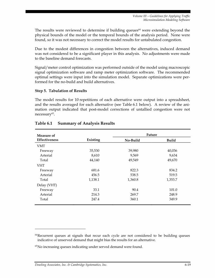
Volume III – Guidelines for Applying Traffic Microsimulation Modeling Software
Dowling Associates, Inc. & Cambridge Systematics, Inc. 6-19
The results were reviewed to determine if building queues64 were extending beyond the physical bounds of the model or the temporal bounds of the analysis period. None were found, so it was not necessary to correct the model results for untabulated congestion.
Due to the modest differences in congestion between the alternatives, induced demand was not considered to be a significant player in this analysis. No adjustments were made to the baseline demand forecasts.
Signal/meter control optimization was performed outside of the model using macroscopic signal optimization software and ramp meter optimization software. The recommended optimal settings were input into the simulation model. Separate optimizations were per-formed for the no-build and build alternatives.
Step 5. Tabulation of Results
The model results for 10 repetitions of each alternative were output into a spreadsheet, and the results averaged for each alternative (see Table 6.1 below). A review of the ani-mation output indicated that post-model corrections of untallied congestion were not necessary65.
Table 6.1 Summary of Analysis Results
Future Measure of Effectiveness Existing No-Build Build VMT
Freeway 35,530 39,980 40,036 Arterial 8,610 9,569 9,634 Total 44,140 49,549 49,670
VHT Freeway 681.6 822.3 834.2 Arterial 456.5 538.5 519.5 Total 1,138.1 1,360.8 1,353.7
Delay (VHT) Freeway 33.1 90.4 101.0 Arterial 214.3 269.7 248.9 Total 247.4 360.1 349.9
64 Recurrent queues at signals that recur each cycle are not considered to be building queues
indicative of unserved demand that might bias the results for an alternative. 65 No increasing queues indicating under served demand were found.

Volume III – Guidelines for Applying Traffic Microsimulation Modeling Software
6-20 Dowling Associates, Inc. & Cambridge Systematics, Inc.
Step 6. Evaluation of Alternatives
Under the no-build scenario, the total delay on the corridor increased by 46 percent over existing conditions. The VMT increased by 12 percent and the total travel time by 20 percent. Most of the delay increases were on the freeway mainline links.
Under the improved scenario (ramp metering plus signal optimization), system wide delay was reduced by about three percent (from the no-build scenario) with a slight increase in VMT66. Freeway mainline traffic conditions improved at the expense of the on-ramp traffic.
The improvements are operationally acceptable (no spillbacks from the ramp meters to the arterial network).
66 The improvement is modest enough that it might be worth establishing confidence intervals for
the results and performing some sensitivity analysis and hypothesis tests to confirm the robustness of the conclusion.

Volume III – Guidelines for Applying Traffic Microsimulation Modeling Software
Dowling Associates, Inc. & Cambridge Systematics, Inc. 7-1
7.0 Final Report
This chapter discusses the documentation of the microsimulation analysis results in a final report and the technical report or appendix supporting the final report.
7.1 The Final Report
The final report presents the assumptions, analytical steps, and results of the analysis in sufficient detail for decision-makers to understand the basis for and impli-cations of choosing among the project alternatives. The Final Report, however, will not usually contain suffi-ciently detailed information to enable other analysts to reproduce the results. That is the purpose of the Technical Report.
The effort involved in summarization of the results should not be under-estimated, since microsimulation models produce a wealth of numerical output that must be tabulated and summarized. The Final Report should include the following:
1. Study Objectives and Scope;
2. Overview of Study Approach (tools used, methodology, rationale);
3. Data Collection (sources and methods);
4. Calibration Tests and Results (which parameters modified and why);
5. Forecast Assumptions (assumed growth inside and outside of study area, street improvements, etc.);
6. Description of Alternatives; and
7. Results.
Working ModelBefore Calibration
4
7
Error Checking
1 Scope Project
2 Data Collection
3 Base Model Development
Work prior toactual modeling
Initial modeling
YesCalibrated Model
5Compare ModelMOE’s to FieldData
Calibration
6 Alternatives Analysis
Adjust Model Parameters
Final Report
AcceptableMatch?
No
ModelApplication

Volume III – Guidelines for Applying Traffic Microsimulation Modeling Software
7-2 Dowling Associates, Inc. & Cambridge Systematics, Inc.
7.2 Technical Appendix
The Technical Appendix documents the microsimulation analysis in sufficient detail to enable an analyst to reproduce the results, including version or release of the software used. It may be an appendix to the final report or a separate document.
The Technical Appendix is a vital step to preserve the rationale for the various decisions that are made in the process of developing, calibrating, and operating a microsimulation model. The documentation should be sufficient, so that given the same input files, another analyst can understand the calibration process and repeat the alternatives analysis.
The Technical Report/Appendix should include the model input files and output files (in electronic format) for the final model calibration run and alternatives analysis model runs. In addition to a diskette with the calibration and alternatives analysis files (input and out-put), the Technical Appendix should include a printed listing of the files on the diskette with a text description of the contents and purpose of each file.
Volume III – Guidelines for Applying Traffic Microsimulation Modeling Software
Dowling Associates, Inc. & Cambridge Systematics, Inc. A-1
Appendix A. Traffic Microsimulation Fundamentals
This section provides an overview of the technical aspects of microsimulation. It identifies and defines the terminology typically used, and what model types and procedures are generally employed in microsimulation. The section also provides a general introduction to traffic simulation models. Readers interested in additional detail on technical aspects of microsimulation may consult Chapter 10: Traffic Simulation in the Revised Monograph on Traffic Flow Theory or other documents.
A.1 Overview
Simulation models are designed to emulate the behavior of traffic in a transportation net-work over time and space to predict the system performance. Simulation models include mathematical and logical abstractions of real-world systems, implemented in computer software. Simulation model runs can be viewed as experiments performed in the labora-tory rather than in the field.
A.2 System Update Mechanism
Traffic simulation models describe the changes in the system state through discrete inter-vals in time. There are generally two types of models, depending if the update time inter-vals are fixed or variable:
• Discrete time (time scan) models – The system being updated at fixed-time intervals. For example, the model calculates the vehicle position, speed and acceleration at 1 sec-ond intervals. The choice of the update time interval depends on how accurately the system needs to be simulated at the expense of computer processing time. Most microsimulation models employ a 0.1 second resolution for updating the system. Traffic systems are typically modeled using time-scan models, because experience a continuous change in state.
• Discrete event (event scan) models – In these models, the time intervals vary in length and correspond to the intervals between events. For example, a pre-timed traffic sig-nal indication (e.g., green) remains constant for 30 seconds until its state changes

Volume III – Guidelines for Applying Traffic Microsimulation Modeling Software
A-2 Dowling Associates, Inc. & Cambridge Systematics, Inc.
instantaneously to yellow. The operation of the signal is described by recording its changes in state when events occur, rather than monitoring the state of the signal each second. Event scanning models typically achieve significant reductions in computer run time. However, they are suitable for simulating systems whose states change infrequently.
A.3 Traffic Stream Representation
Simulation models are typically classified according to the level of detail at which they represent the traffic stream. These include:
• Microscopic models – Simulate the characteristics and interactions of individual vehi-cles. They essentially produce trajectories of vehicles as they move through the net-work. The processing logic includes algorithms and rules describing how vehicles move and interact, including acceleration, deceleration, lane changing, and passing maneuvers.
• Mesoscopic models – Simulate individual vehicles but describes their activities and interactions based on aggregate (macroscopic) relationships. Typical applications of mesoscopic models are evaluations of traveler information systems. For example, they can simulate the routing of individual vehicles equipped with in-vehicle real time travel information systems. The travel times are determined from the simulated aver-age speeds on the network links. The average speeds are in turn calculated from a speed-flow relationship.
• Macroscopic models – Simulate traffic flow considering aggregate traffic stream char-acteristics (speed, flow, density) and their relationships. Typically macro models employ equations on the conservation of flow and on how traffic disturbances (shock waves) propagate in the system. They can be used to predict the spatial and temporal extent of congestion due to traffic demand or incident conditions in a network, but cannot model the interactions of vehicles on alternative design configurations.
Microscopic models are potentially more accurate than macroscopic simulation models. However, they employ many more parameters that require calibration. Also, the parameters of macroscopic models (e.g., capacity) are observable in the field. Most of the parameters of microscopic models cannot be observed directly in the field (e.g., minimum distances between vehicles in car-following situations).
A.4 Randomness in Traffic Flow
Simulation models are also classified depending on how they represent the randomness in traffic flow, including:
Volume III – Guidelines for Applying Traffic Microsimulation Modeling Software
Dowling Associates, Inc. & Cambridge Systematics, Inc. A-3
• Deterministic models – Assume that there is no variability in the driver-vehicle char-acteristics. For example, it is assumed that all drivers have a critical gap of five sec-onds to merge into a traffic stream, or all passenger cars have a vehicle length of 16 feet.
• Stochastic models – Assign driver–vehicle characteristics from statistical distributions using random numbers. For example, the desired speed of a vehicle is randomly gen-erated from an assumed normal distribution of desired speeds with mean of 65 mph and standard deviation of five mph. Stochastic simulation models have routines that generate random numbers. The sequence of random numbers generated depends on the particular method and the initial value of the random number (random number seed). Changing the random number seed produces a different sequence of random numbers which in turn produces different values of driver-vehicle characteristics.
Stochastic models require additional parameters to be specified (e.g., the form and parameters of the statistical distributions to represent the particular vehicle character-istic). More important the analysis of the simulation output should consider that the results from each model run vary with the input random number seed for otherwise identical input data. Deterministic models in contrast, will always produce the same results with identical input data.
A.5 The Microsimulation Process
Microsimulation models employ several submodels, analytical relationships and logic to model traffic flow. Detailed description of each submodel is beyond the scope of this sec-tion. Instead, this document focuses on some key aspects of the simulation process that are likely to affect the choice of the particular tool to be used and the accuracy of the results.
Simulation models include algorithms and logic to:
• Generate vehicles into the system to be simulated;
• Move vehicles into the system; and
• Model vehicle interactions.
A.5.1 Vehicle Generation
A.5.1.1 Generating Vehicles into the Traffic Stream
At the beginning of the simulation run, the system is “empty”. Vehicles are generated at the entry nodes of the analysis network, based on the input volumes and an assumed headway distribution. Suppose the specified volume is V=600 vph for a 15-minute analysis
Volume III – Guidelines for Applying Traffic Microsimulation Modeling Software
A-4 Dowling Associates, Inc. & Cambridge Systematics, Inc.
period, and the model uses a uniform distribution of vehicle headways. Then a vehicle will be generated at time intervals:
H = Mean headway = 3600/V = 3600/600 = 6 seconds
If the model uses the shifted negative exponential distribution to simulate the arrival of vehicles at the network entry node, instead of the uniform distribution, then vehicles will be generated as time intervals:
h - H +R)] - (1 [- )h - (H = h minmin ln
Where:
h = headway (sec) separating each generated vehicle;
hmin = Specified minimum headway (e.g., 1.0 sec); and
R = Random number (0 to 1.0).
A.5.1.2 Generating Driver-Vehicle Attributes
When a vehicle is generated at the entry of the network, the simulation model assigns driver-vehicle characteristics. The following characteristics or attributes are commonly generated for each driver/vehicle unit:
• Vehicle – Type (car, bus, truck), length, width, maximum acceleration and decelera-tion, maximum speed, maximum turn radius, etc.; and
• Driver – Driver aggressiveness, reaction time, desired speed, critical gaps (for lane changing, merging, crossing), destination (route), etc.
Note that different models may employ additional attributes for each driver/vehicle unit to improve the realism that the model replicates real-world conditions. Each attribute may be represented in the model by constants (e.g., all passenger cars have a vehicle length of 16 feet), functional relationships (e.g., maximum vehicle acceleration is a linear function of its current speed), or probability distributions (e.g., driver’s desired speed is obtained from a normal distribution). Most microsimulation models employ statistical distributions to represent the driver/vehicle attributes. The statistical distributions employed to represent the variability of the driver/vehicle attributes and their parameters must be calibrated to reflect local conditions.
Figure A.1 illustrates a generic process for generating driver/vehicle attributes for a sto-chastic microscopic simulation model. Drivers are randomly assigned an “aggressiveness index” ranging from 1 (very aggressive) to 10 (very cautious) drawn from a uniform dis-tribution to represent the range of human behavior. Once the value of aggressiveness has been assigned (X=7 in this example), it is used to assign the value of free-flow speed (=97 kph), and acceptable deceleration (-11 fps2) from the corresponding distributions of speeds and accelerations.

Volume III – Guidelines for Applying Traffic Microsimulation Modeling Software
Dowling Associates, Inc. & Cambridge Systematics, Inc. A-5
Figure A.1 Generation of Driver Characteristics
Source: Traffic Flow Theory Monograph, Chapter 10: Simulation.
Volume III – Guidelines for Applying Traffic Microsimulation Modeling Software
A-6 Dowling Associates, Inc. & Cambridge Systematics, Inc.
A.5.2 Vehicle Movements
This section briefly describes the process for simulating vehicle movements and how they are impacted by the physical environment. The physical environment, the transportation network under study, is typically represented as a network of links and nodes. Links are one-way roadways with fixed design characteristics and nodes represent intersections or locations where the design characteristics of the links change. Simulation models have different limits on the network size (maximum number of links and nodes).
Vehicles in the absence of impedance from other vehicles travel at their desired speed on the network links. However, their speed may be affected by the link-specified geometry (horizontal and vertical alignment), pavement conditions, and other factors. For example, the simulation model computes the actual vehicle speed as the minimum value from the desired speed and the speed computed for the specified vertical and horizontal alignment. However, not all microsimulation tools model the sensitivity of vehicle speeds to link design characteristics.
Vehicles proceed through the network until they exit the system at their destination. Typically, there are two types of simulation models: “turning fraction” based or “O-D based.” In O-D-based models, the origin-destination matrix is input, and when a vehicle is generated at an origin, it is assigned its destination. The vehicle then exits the network at the specified destination. In turning fraction-based models, the vehicle destination is ran-domly assigned at the entry of the link based on specified turning volumes (or fractions) at the downstream end of the link. For example, for a vehicle entering a signalized inter-section approach, the vehicle destination (going through or turning) is randomly deter-mined based on the input turning volume fractions for the particular link. This also implies that turning-fraction models are not well suited for tracing the performance of individual vehicles throughout the network and evaluating the effectiveness of certain ITS options (e.g., a fraction of vehicles being equipped with real-time information systems).
Simulation models employ a number of approaches to “guide” vehicles within the net-work. They typically employ “warning signs” to advise the simulated vehicle to change lanes, because it needs to exit at the downstream off-ramp, its lane is ending, or there is a blockage downstream. The location of warning signs may significantly affect the accuracy of the simulation. For example, vehicles traveling on the freeway at a speed of 60 mph (88 feet per sec) may miss their exit without advance warning if they are traveling at the median lane of a multilane freeway and are required to make multiple lane changes to exit at the downstream end of a short link.
A.5.2.1 Vehicle Interactions
Microscopic models simulate the interactions of individual vehicles as they travel in the analysis network using car-following, lane-changing and queue discharge algorithms.

Volume III – Guidelines for Applying Traffic Microsimulation Modeling Software
Dowling Associates, Inc. & Cambridge Systematics, Inc. A-7
A.5.2.2 Car-Following
The interaction between a leader and follower pair of vehicles traveling in the same lane, is generally assumed to be a form of a stimulus-response mechanism:
Response follower (t+T) = (sensitivity) * (stimulus) t
Where:
T is the reaction time (time lag) for the response of the following vehicle.
Car-following models for highway traffic were proposed since the inception of traffic flow theory in the early 1950’s. Extensive experimentation and theoretical work was per-formed at the General Motors (GM) laboratories and elsewhere. Most of the existing simulation models employ “fail-safe” car-following algorithms. Such algorithms simulate car-following behavior by maintaining minimum safety distance between vehicles subject to stochastically generated vehicle characteristics (e.g., maximum acceleration and decel-eration rates). The “fail-safe” car-following algorithms currently implemented in most simulation models consist of the following components:
a. An equation which calculates the acceleration (deceleration) of the following vehicle in response to the motion of its leader, to maintain a target headway (spacing) depending on the driver-vehicle characteristics.
) X ,T , s ,v ,v( F = a iflf
Where:
af is the acceleration of the following vehicle after a reaction time, T;
Vl and Vf are the speeds of the leading and following vehicles;
s is the distance between vehicles; and
Xi are parameters specific to the particular car-following model.
b. The above computed acceleration rate must not exceed the maximum acceleration rate for the specific vehicle type and must not result in a higher speed than the vehicle’s desired speed.
c. Furthermore, the computed acceleration of the follower (a) must satisfy the “safe-fol-lowing” rule (i.e., the follower should always maintain a minimum separation from the leader). If the value of the safe-following acceleration is smaller then the car-following acceleration computed in (a), the former is implemented.

Volume III – Guidelines for Applying Traffic Microsimulation Modeling Software
A-8 Dowling Associates, Inc. & Cambridge Systematics, Inc.
A.5.2.3 Lane Changing
The modeling of lane-changing is based on the gap-acceptance process. A vehicle may change lanes if the available gap in the target lane is greater than its critical gap. Typi-cally, three types of lane changes are modeled:
1. Mandatory lane-change, where a vehicle is required to exit the current lane. Merging from an on-ramp to the freeway is an example of a mandatory lane change. A vehicle must execute a lane-change under several circumstances:
a. The current lane is ending (lane drop);
b. Move to the outer lane(s) to exit the freeway via an off-ramp;
c. The current lane will not “accommodate” its movement or vehicle type (e.g., HOV lane); or
d. The lane is blocked because of incidents or other events.
2. Discretionary lane change, where a vehicle changes lanes to improve its position (i.e., travel at the desired speed). If a driver is impeded in the current lane because of a slower moving vehicle in front, he may consider changing lanes to improve his posi-tion (i.e., resume his desired speed). The lane-changing logic determines which of the adjacent lanes (if more than one is available) is the “best candidate.” To be a candi-date, the lane’s channelization must accommodate the subject vehicle, be free of a blockage and not end close by. The lane changing is performed subject to the avail-ability of gaps in the candidate lane and the acceptability of the gaps by the subject vehicle.
On a surface street network, discretionary lane changes may occur because of various impedance factors perceived by the driver, including:
a. Queue length at the stop-line;
b. Heavy truck traffic;
c. Bus transit operations;
d. Turn movements from shared lanes;
e. Pedestrian interference with turning vehicles; and
f. Parking activities.
3. Anticipatory lane change, where a vehicle may change lanes in anticipation of slow downs in its current lane further downstream as a result of merging or weaving. The decision to change lanes is based on the difference in speed at the location of the merge or weave, between vehicles in the current lane and the adjacent lane not directly involved in the merge or weave. The lane changing logic recognizes that a driver may accelerate or decelerate to “create” acceptable gaps in order to change lanes. Consider a vehicle A which desires to merge into a gap between vehicles B and C (B currently is the leader of C). Vehicle A will accept the gap if the time headway between himself and vehicle B is greater than some critical value g(A,B) and the time headway between

Volume III – Guidelines for Applying Traffic Microsimulation Modeling Software
Dowling Associates, Inc. & Cambridge Systematics, Inc. A-9
himself and the vehicle C is greater than some critical value g(A,C). However, the critical time headway values are not constant but are dependent on the following considerations:
− The critical time headways depend on the vehicle speeds. Vehicle A will accept a smaller critical headway if it is going slower than vehicle B, than if it is going faster than vehicle B.
− The lane change takes place over a finite period of time. During this time period the lane changer can adjust his position with respect to the new leader by decelerating.
− The new follower may cooperate with the lane changer by decelerating to increase the size of the gap.
These considerations are typically combined in a risk measure. More aggressive drivers would accept a higher risk value (i.e., shorter gaps and higher accelera-tion/deceleration rates) to change lanes. Moreover, the risk value may be further increased depending on the type of lane change and the situation. For example, a merging vehicle reaching the end of the acceleration lane may accept much higher risk values (“forced lane changes”).
The model’s lane changing logic and parameters have important implications on traffic performance, especially for freeway merging and weaving areas. In addition, the time assumed to complete the lane change maneuver affects the traffic performance, because the vehicle occupies both lanes (original and target lane) during this time interval. Fur-thermore, one lane change is allowed per simulation time interval.

Volume III – Guidelines for Applying Traffic Microsimulation Modeling Software
Dowling Associates, Inc. & Cambridge Systematics, Inc. B-1
Appendix B. Confidence Intervals
This appendix explains how to compute the confidence intervals for microsimulation model results. It explains why and how to compute the minimum number of repeated field measurements or microsimulation model runs needed to estimate the mean with a certain level of confidence that the true mean actually falls within a target interval.
Three pieces of information are required: The sample standard deviation, the desired length of the confidence interval, and the desired level of confidence.
The required number of repetitions must be estimated by an iterative process. A prelimi-nary set of repetitions is usually required to make the first estimate of the standard devia-tion for the results. The first estimate of the standard deviation is then used to estimate the number of repetitions required to make statistical conclusions about alternative high-way improvements.
When all of the repetitions have been completed, the analyst then goes back and recom-putes the standard deviation and required number of repetitions, based upon all of the completed repetitions. If the required number of repetitions is less than or equal to the completed number of repetitions, then the analysis is complete. If not, then the analyst either relaxes the desired degree of confidence in the results or performs additional repetitions.
B.1 Why Are Multiple Model Runs Required?
Multiple repetitions of the same model are required because microsimulation results will vary depending upon the random number seed used in each run. The random number seed is used to select a sequence of random numbers, which are used to make numerous decisions throughout the simulation run (Should a vehicle be loaded on the network this second, or later? Should the driver be aggressive or timid? Which vehicle type should it be? Will the driver choose the shortest path or a slightly longer one instead?). The out-comes of all of these decisions will affect the simulation results. The results of each run will usually be close to the average of all the runs, but each run will be different than the other.
Figure B.1 illustrates the range of results that can occur simply by varying the random number seed used in each run. The figure shows the mean sys-tem vehicle speed for a freeway-to-freeway inter-change during each minute of the simulation run. A total of six simulation runs (called
Microsimulation model results can vary by 25 percent between runs.

Volume III – Guidelines for Applying Traffic Microsimulation Modeling Software
B-2 Dowling Associates, Inc. & Cambridge Systematics, Inc.
processes in the figure) were made. As can be seen, after the initial warm-up period, results diverge. The range of mean speeds output by each process is about five to six mph for most of the length of the simulation period. Running a longer simulation period does not reduce this variation. At the end of the simulation, the range of results is about six mph, or 25 percent of the mean system speed at the end of the simulation period.
Figure B.1 Variation in Results Between Repetitions
Vehicle Mean Speed
0
10
20
30
40
50
60
70
16:21
16:24
16:27
16:30
16:33
16:36
16:39
16:42
16:45
16:48
16:51
16:54
16:57
17:00
17:03
17:06
17:09
17:12
17:15
17:18
17:21
17:24
17:27
17:30
Simulation Time
mph
process-001process-002process-003process-004process-005process-006
Source: I-580/I-680 Freeway Interchange Model, Dowling Associates, 2002.
B.2 Estimation of Sample Standard Deviation
The standard deviation (an estimate of the variance) is required to estimate the number of repetitions. However, it takes a minimum number of repetitions to estimate the standard deviation in the first place. So either the analyst estimates the standard deviation directly (based upon past experience) or executes a few model run repetitions (each run using a different random number seed) and uses the equation below to compute an initial esti-mate of the sample standard deviation.
Volume III – Guidelines for Applying Traffic Microsimulation Modeling Software
Dowling Associates, Inc. & Cambridge Systematics, Inc. B-3
( )1
2
2
−
−= ∑
Nxx
s
Where:
s = the standard deviation;
x = the variable (such as delay) for which the sample variance is desired;
x = the average value of the variable produced by the model runs; and
N = number of model runs.
Unless the analyst already knows from experience the standard deviation, it is recom-mended that four repetitions be performed for the initial estimation of the standard deviation. This initial estimate is then revisited and revised later if and when additional repetitions are performed for the purposes of obtaining more precise estimates of mean values or for alternatives analysis.
B.3 Selection of Desired Confidence Level
The confidence level is the probability that the true mean lies within the target confidence interval. The analyst must decide to what degree he or she wishes to know the interval in which the true mean value lies. The usual approach is to pick a 95 percent level of confi-dence, but analysts may choose higher or lower levels of confidence. Higher percent lev-els of confidence require more repetitions.
B.4 Selection of Desired Confidence Interval
The confidence interval is the range of values within which the true mean value may lie. The length of the interval is at the discretion of the analyst and may vary according to the purpose for which the results will be used. For example, if the analyst is testing alterna-tives that are very similar, then a very small confidence interval will be desired to distin-guish between the alternatives. If the analyst is testing alternatives with big differences, then a larger confidence interval can be tolerated. Smaller confidence intervals require more repetitions to achieve a given level of confidence. Confidence intervals less than half

Volume III – Guidelines for Applying Traffic Microsimulation Modeling Software
B-4 Dowling Associates, Inc. & Cambridge Systematics, Inc.
the value of the standard deviation will require a large number of repetitions to achieve reasonable confidence levels.67
B.4.1 Computation of Minimum Repetitions
It is impossible to know in advance exactly how many model runs will be needed to determine a mean (or any other statistical value) to the analyst’s satisfaction. However, after a few model runs, the analyst can make an estimate of how many more runs may be required to obtain a statistically valid result.
The required minimum number model repetitions is computed using the following equation:
NstCI N 1),2/1(%1 2 −−− ∗= αα
Where:
CI(1-alpha)% = the (1-alpha)% confidence interval for the true mean, where “alpha” equals the probability of the true mean not lying within the confidence interval;
t(1-alpha/2),N-1 = the Student’s “t” statistic for the probability of two-sided error summing to “alpha” with N-1 degrees of freedom, where “N” equals the number of repetitions; and
s = the standard deviation of the model results.
Note that when solving this equation for “N,” it will be necessary to iterate until the esti-mated number of repetitions matches the number of repetitions assumed when looking up the “t” statistic. Table B.1 shows the solutions to the above equation in terms of the mini-mum number of repetitions for various desired confidence intervals and desired degrees of confidence.
67With such a tight confidence interval, the analyst may be striving for a degree of precision not
reflected in real-world conditions.

Volume III – Guidelines for Applying Traffic Microsimulation Modeling Software
Dowling Associates, Inc. & Cambridge Systematics, Inc. B-5
Table B.1 Minimum Repetitions to Obtain Desired Confidence Interval
Desired Range (CI/S)
Desired Confidence
Minimum Repetitions
0.5 99% 130 0.5 95% 83 0.5 90% 64 1.0 99% 36 1.0 95% 23 1.0 90% 18 1.5 99% 18 1.5 95% 12 1.5 90% 9 2.0 99% 12 2.0 95% 8 2.0 90% 6
Notes: 1. Desired Range = desired confidence interval (CI) divided
by standard deviation (S); and 2. For example, if the standard deviation in the delay is
1.5 seconds and the desired confidence interval is 3.0 seconds at a 95 percent confidence level, then it will take eight repetitions to estimate the mean delay to within plus or minus 1.5 seconds.
Volume III – Guidelines for Applying Traffic Microsimulation Modeling Software
Dowling Associates, Inc. & Cambridge Systematics, Inc. C-1
Appendix C. Estimation of the Simulation Initialization Period
Simulation model runs usually start with zero vehicles on the network. If the simulation output is being compared to field measurements (as in calibration), then the artificial period where the simulation model starts out with zero vehicles (the warm-up period) must be excluded from the reported statistics for system performance. Some software packages will do this automatically. For others, the warm-up period must be computed off-line by the analyst. This appendix explains how to identify the warm-up period.
The number of vehicles present at any one time on the network is used to determine if the model has reached equilibrium and therefore can start tallying performance statistics for the network. Once the number of vehicles present on the network ceases to increase by a minimum specified amount, then the warm-up period is deemed to be concluded (see Figure C.1).
If the number of vehicles and the mean speed do not level off within the first 15 minutes, it could be that the demand coded by the analyst for the system is greater than the system capacity. In this case, congestion will never level off. This will result in less accurate con-gestion statistics since the system never clears the congestion. The analyst should consider extending the starting and end times of the simulation to incorporate lower demand peri-ods before and after the peak period.
If it is not feasible to extend the simulation period to uncongested time periods, the ana-lyst should choose a warm-up period that is equal to at least twice the estimated travel time at free-flow conditions to traverse the length of the network. For example, if the freeway being modeled is five miles long, it takes roughly five minutes to traverse the length of it at free-flow speed, so the warm-up period is set at 10 minutes.
Note that in this example, the number of vehicles in the system is generally steadily increasing. The system never reaches equilibrium. Initialization is achieved when the number of vehicles entering the system are approximately equal to the number leaving the system (even though this slight decline is later superceded by larger increases). The gen-erally increasing trend in the number of vehicles present in the system suggests that the simulation period be extended earlier and later to incorporate lower demand periods at the beginning and the end of the peak period.

Volume III – Guidelines for Applying Traffic Microsimulation Modeling Software
C-2 Dowling Associates, Inc. & Cambridge Systematics, Inc.
Figure C.1 Illustration of Warm-Up Period
0
500
1000
1500
2000
2500
16:21
:00
16:24
:00
16:27
:00
16:30
:00
16:33
:00
16:36
:00
16:39
:00
16:42
:00
16:45
:00
16:48
:00
16:51
:00
16:54
:00
16:57
:00
17:00
:00
17:03
:00
17:06
:00
17:09
:00
17:12
:00
17:15
:00
17:18
:00
17:21
:00
17:24
:00
17:27
:00
17:30
:00
Simulation Time
Num
ber o
f Veh
icle
s in
Sys
tem
Warm-up Period = 20 minutes
Source: I-680/I-580 Interchange Microsimulation Model, Dowling Associates, 2002.

Volume III – Guidelines for Applying Traffic Microsimulation Modeling Software
Dowling Associates, Inc. & Cambridge Systematics, Inc. D-1
Appendix D. Simple Search Algorithms for Calibration
Since simulation models are complex models, it is not typically possible to formulate the models as a closed form equation for which traditional calculus techniques can be applied to find a minimum value solution. It is necessary to use some sort of search algorithm that relies upon multiple operations of the simulation model, plotting of the output results as points, and searching between these points for the optimal solution. Search algorithms are required to find the optimal solution to the calibration problem. The calibration problem is a “non-linear,” “least-squares” optimization problem.
There are many software packages available for identifying the optimal combination of calibration parameters for minimizing the squared error between the field observations and the simulation model. The Argonne National Laboratory (http://www-fp.mcs.anl.gov/otc/Guide/SoftwareGuide/Categories/nonlinleastsq.html) lists several software packages for “non-linear least squares” parameter estimation.
The sections below illustrate some simple approaches available for single parameter esti-mation and dual parameter estimation when working with a standalone simulation model. Estimation of three or more parameters however; would require the use of software.
D.1 Single Parameter Search Algorithm (Golden Section)68
Several methods are available for finding the value of a single parameter that minimizes the squared error between the model and the observations. These methods include Newton’s Method, Secant Method, Quadratic Approximation Methods, and the Golden Section Method. The Golden Section Method is illustrated in the example below.
68 References: F. S. Hillier, G. J. Lieberman, Introduction to Operations Research, Sixth Edition,
McGraw-Hill, New York, 1995; H. A. Taha, Operations Research, An Introduction, Seventh Edition, Prentice-Hall, New York, 2003 (If seventh edition is not available, look for sixth edition published in 1996.).

Volume III – Guidelines for Applying Traffic Microsimulation Modeling Software
D-2 Dowling Associates, Inc. & Cambridge Systematics, Inc.
D.1.1 Example of Golden Section Method
Objective: Find the global value of the mean headway between vehicles that minimizes the squared error between field counts of traffic volumes and model estimates.
Approach: Use the Golden Section Method to identify the optimal mean headway.
Step 1. Identify the maximum and minimum acceptable values for the parameter to be optimized
This step brackets the possible range of the parameter in which the optimal solution is presumed to lie. The user can select the appropriate range. For this example, we will set the minimum acceptable value for the mean headway at 0.5 seconds and the maximum at 2.0 seconds. The larger the range, the more robust we search. However, it will take longer to find the optimum value. The smaller the range of acceptable values, the greater the likelihood that the best solution lies outside the range.
Step 2. Compute squared error for maximum and minimum values
The simulation model is run to determine the volumes predicted when the maximum acceptable mean headway is input, and again for the minimum acceptable headway. Either randomization should be turned off, or the model should be run several times with each mean headway and the results averaged. The squared error produced by the model for each mean headway is computed.
Step 3. Identify two interior parameter values for testing
The two interior points (x1 and x2) are selected according to specific ratios of the total range that preserve these ratios as the search range is narrowed in subsequent iterations. The formulae for selecting the two interior mean delays for testing are the following:
min)(max382.0min1 −•+=x
min)(max618.0min2 −•+=x
Where:
x1 = the lower interior point value for the mean delay to be tested;
x2 = the upper interior point value for the mean delay to be tested;
min = the lower end of the search range for the mean delay; and
max = the upper end of the search range for the mean delay.
The minimum and maximum ends of the search range are initially set by the user (based on the acceptable range set in Step 1), but then the search range is gradually narrowed as each iteration is completed.

Volume III – Guidelines for Applying Traffic Microsimulation Modeling Software
Dowling Associates, Inc. & Cambridge Systematics, Inc. D-3
Figure D.1 Golden Section Method
0 Min Maxx1 x2
Squa
red
Erro
r
Search Range
Parameter
Step 4. Compute squared error for two interior parameter values
The simulation model is run for the new values of mean delay (x1 and x2) and the squared errors are computed.
Step 5. Identify the three parameter values which appear to bracket the optimum
This step narrows the search range. The parameter value (x1 or x2) that produces the lowest squared error is identified. (If either the minimum or the maximum parameter values produce the least squared error, the search range should be reconsidered.) The parameter values to the left (lower) and right (higher) of that point become the new mini-mum and maximum values for the search range. For instance, in Figure D.1, parameter value x2 produces the lowest squared error.
Step 6. Go to Step 3, repeat until uncertainty in location of optimal parameter value is satisfactory
The golden section search is repeated until the range of values in which the optimum parameter value lies is small enough to satisfy the user’s requirements. After about 10 iterations, the uncertainty in the optimal value of the parameter is reduced by a factor of 100. Therefore, if an initial range of 0.5 to 2.5 is specified for the mean headway (a range of 2.0 seconds), this range will be reduced to 0.2 seconds after 10 iterations of the golden section method. The user should obtain the optimal value of the mean headway to within plus or minus one tenth of one second.

Volume III – Guidelines for Applying Traffic Microsimulation Modeling Software
D-4 Dowling Associates, Inc. & Cambridge Systematics, Inc.
D.2 Simple Two Parameter Search Algorithm
In the case where two model parameters are to be optimized, a contour plot approach to identifying the optimal values of the parameters can be utilized. One first identifies the acceptable ranges of the two parameters and then exercises the model for pairs of values of the parameters. The squared error is computed for each pair of parameter values and plotted in a contour plot to identify the value pairs that result in the lowest squared error. An example of this approach is shown in Figure D.2 for optimizing the mean headway and mean reaction time parameters. The search starts with the default values, blankets the region with a series of tests of different values, and then focuses in more detail on the solution area.
Figure D.2 Example Contour Plot of Squared Error
0
Mea
n H
eadw
ay
Mean Reaction Time
3.8
3.1
3.2
2.1
2.81.6
3.2
3.8
3.5
0.6
0.8
0.5
0.71.3
3.2
3.4
Default
Def
ault
3
2
1
Contours = Squared Error x 105
Optimal Headway
Opt
imal
Rea
ctio
n Ti
me

Volume III – Guidelines for Applying Traffic Microsimulation Modeling Software
Dowling Associates, Inc. & Cambridge Systematics, Inc. D-5
D.3 A Dual Objective, Two Parameter Search Algorithm69
This section addresses the case where the analyst wishes to consider two model calibra-tion objectives separately, rather than as the weighted sum of the square errors (single objective) discussed above. The analyst in this case can use a variation of the two-dimensional search algorithm identified above with up to two parameters. Instead of plotting a single set of contour lines for the squared error, the analyst plots two sets of contour lines (one set for each objective) for each pair of parameters. The analyst then visually identifies the acceptable solution range where both objectives are satisfied to the extent feasible. The following example illustrates this algorithm.
The analyst has identified the following two objectives for the model calibration:
1. The model should predict a mean speed of the freeway of 35 mph (plus or minus two mph); and
2. The model should predict the maximum observed flow rate for the bottleneck section to be 2,200 vehicles per hour per lane (plus or minus 100 vph).
Figure D.3 shows how changing the mean headway and the mean reaction time changes the values of these two objectives (speed and capacity). The solution region shows the pairs of values of mean headway and mean reaction time that meet both objectives.
69 Adapted from Gardes, Y., A. D. May, J. Dahlgren, A. Skabardonis, Bay Area Simulation and Ramp
Metering Study, UCB-ITS-PRR-2002-6 California PATH Research Report, University of California, Berkeley, February 2002.

Volume III – Guidelines for Applying Traffic Microsimulation Modeling Software
D-6 Dowling Associates, Inc. & Cambridge Systematics, Inc.
Figure D.3 Dual Objective, Dual Parameter Search
0
Mea
n H
eadw
ay
Mean Reaction Time
Default
Def
ault
Solution Region
Speed = 25 mph
Speed = 30 mph
Speed = 35 mph
Capacity = 2400 vphl
Capacity = 2200 vphl Capacity = 2000 vphl

Volume III – Guidelines for Applying Traffic Microsimulation Modeling Software
Dowling Associates, Inc. & Cambridge Systematics, Inc. E-1
Appendix E. Hypothesis Testing of Alternatives
When the microsimulation model is run several times for each alternative, the analyst may find that the variance in the results for each alternative is close to the difference in the mean results for each alternative. How is the analyst to determine if the alternatives are significantly different? To what degree of confidence can the analyst claim that the observed differences in the simulation results are due to the differences in the alternatives and not just the result of using different random number seeds? This is the purpose of statistical hypothesis testing. Hypothesis testing determines if the analyst has performed an adequate number of repetitions for each alternative to tell the alternatives apart at the analyst’s desired level of confidence.
E.1 Estimation of the Required Number of Model Repetitions
This section identifies how to estimate the minimum number of model run repetitions that would be required to determine if two alternatives with results a given distance apart are significantly different. This estimate however requires a preliminary estimate of the stan-dard deviation of the model run results for the alternatives, which in turn requires some preliminary runs in order to estimate the standard deviation.
The procedure involves the following steps:
1. Perform a preliminary set of model run repetitions for each alternative;
2. Estimate the standard deviation and the mean difference between the alternatives from the preliminary runs, and then compute the required number of runs using the equations in this subsection; and
3. If the required number of runs is greater than the preliminary number of runs, the ana-lyst should perform the additional repetitions for each alternative, and recompute the mean difference and standard deviation using the augmented set of model run repetitions.

Volume III – Guidelines for Applying Traffic Microsimulation Modeling Software
E-2 Dowling Associates, Inc. & Cambridge Systematics, Inc.
E.1.1 Estimation of Pooled Standard Deviation
The analyst should perform about six to eight model repetitions of each alternative to estimate the pooled standard deviation for all alternatives according to the following equation:
22
22yx ss
ps +=
Where:
sx = The standard deviation of model run results for alternative “x”; and
sy = The standard deviation of model run results for alternative “y.”
The preliminary model repetitions used to estimate the pooled estimate of the standard deviation of the model run results can also be used to estimate the likely difference of the means for each alternative.
E.1.2 Selection of Desired Confidence Level
A 95 percent confidence level is often selected for hypothesis testing. This means that there is a five percent chance (often called “alpha” in the textbooks) that the analyst will mistakenly reject the Null Hypothesis when it is really true (Type I error.). If a higher con-fidence level is desired, it comes at the cost of increasing the likelihood of making a Type II error, accepting the null hypothesis when it is really false (Table E.1).
Table E.1 Null Hypothesis
True False
Accept Hypothesis OK Type II Error
Reject Hypothesis Type I Error OK
The study objective may determine the desired confidence level. For example, if the objective is to design an alternative with a 95 percent probability that it will provide sig-nificant improvements over the current facility, then this is the appropriate confidence level for the determination of the number of model repetitions required.

Volume III – Guidelines for Applying Traffic Microsimulation Modeling Software
Dowling Associates, Inc. & Cambridge Systematics, Inc. E-3
E.1.3 Selection of Minimal Difference in Means
The likely minimal difference in means between alternatives should be identified by the analyst. This is the target sensitivity of the simulation tests of the alternatives. Alterna-tives with mean results farther apart than this minimal difference will be obviously differ-ent. Alternatives with mean results closer together than this minimal difference will be considered to be indistinguishable.
The study objectives have some bearing on the selection of the minimal difference to be detected by the simulation tests. If the study objective is to design a highway improve-ment that reduces mean delay by at least 10 percent, then the tests should be designed to detect if the alternatives are at least 10 percent apart.
The preliminary model repetitions used to estimate the pooled estimate of the standard deviation of the model run results can also be used to estimate the likely difference of the means for each alternative. The smallest observed difference in these preliminary runs would be the selected minimal difference of means to be used in determining the required number of repetitions.
E.1.4 Computation of Minimum Repetitions
Assuming that the analyst wishes to reject the null hypothesis that the means of the two most similar alternatives are equal with only an “alpha” percent chance of error against the counter hypothesis that the mean of alternative “x” is different than “y,” then the number of repetitions required can be computed according to the following equation:70
npn styx 222);2/1( •>− −−α
Where:
=− yx The absolute value of the estimated difference between the mean values for the two most similar alternatives “x” and “y”;
sp = The pooled estimate of the standard deviation of model run results for each alternative;
70 If the analyst intends to perform hypothesis tests on only a few pairs of alternatives, then the
equation provided should be sufficiently accurate. However, if the analyst plans to perform hypothesis testing of all possible pairs of alternatives, then this equation will underestimate the required number of repetitions needed to achieve the desired confidence level. The analyst should consult Chapter 12, Introduction to Between Subjects ANOVA, “All pairwise comparisons among means” in D. M. Lane, Hyperstat OnLine, An Introductory Statistics Book and Online Tutorial for Help in Statistics, Rice University (http://www.davidmlane.com/hyperstat).
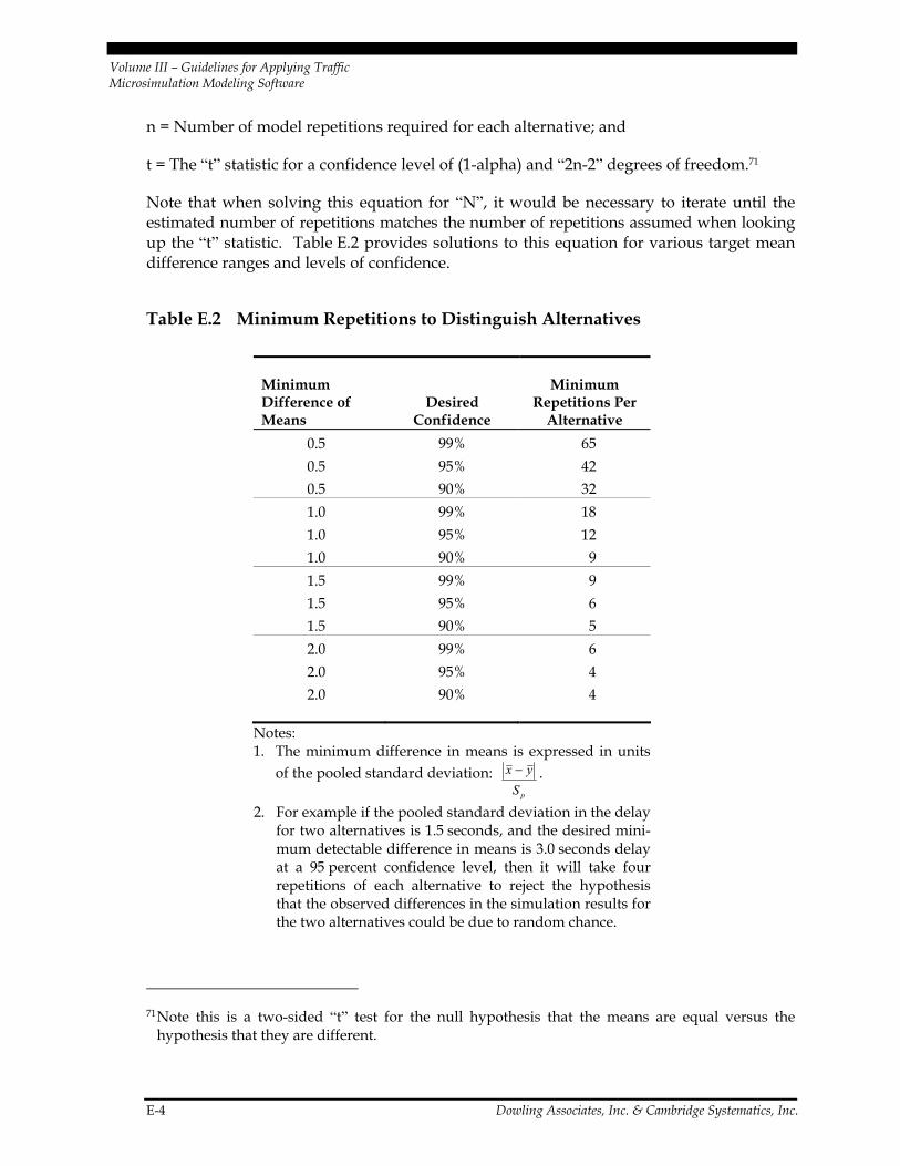
Volume III – Guidelines for Applying Traffic Microsimulation Modeling Software
E-4 Dowling Associates, Inc. & Cambridge Systematics, Inc.
n = Number of model repetitions required for each alternative; and
t = The “t” statistic for a confidence level of (1-alpha) and “2n-2” degrees of freedom.71
Note that when solving this equation for “N”, it would be necessary to iterate until the estimated number of repetitions matches the number of repetitions assumed when looking up the “t” statistic. Table E.2 provides solutions to this equation for various target mean difference ranges and levels of confidence.
Table E.2 Minimum Repetitions to Distinguish Alternatives
Minimum Difference of Means
Desired Confidence
Minimum Repetitions Per
Alternative 0.5 99% 65 0.5 95% 42 0.5 90% 32 1.0 99% 18 1.0 95% 12 1.0 90% 9 1.5 99% 9 1.5 95% 6 1.5 90% 5 2.0 99% 6 2.0 95% 4 2.0 90% 4
Notes: 1. The minimum difference in means is expressed in units
of the pooled standard deviation: pSyx − .
2. For example if the pooled standard deviation in the delay for two alternatives is 1.5 seconds, and the desired mini-mum detectable difference in means is 3.0 seconds delay at a 95 percent confidence level, then it will take four repetitions of each alternative to reject the hypothesis that the observed differences in the simulation results for the two alternatives could be due to random chance.
71 Note this is a two-sided “t” test for the null hypothesis that the means are equal versus the
hypothesis that they are different.

Volume III – Guidelines for Applying Traffic Microsimulation Modeling Software
Dowling Associates, Inc. & Cambridge Systematics, Inc. E-5
E.2 Hypothesis Testing For Two Alternatives
To determine whether simulation outputs provide sufficient evidence that one alternative is better than the other (e.g., Build Project versus No-Build), it is necessary to perform a statistical hypothesis test of the difference of the mean results for each alternative. A null hypothesis is specified, “The model predicted difference in VHT for the two alternatives occurred by random chance. There really is no significant difference in the mean travel time between the alternatives”. A statistic is computed for a selected level of confidence, and if the difference between the two means is less than that statistic, then the null hypothesis is accepted and it is concluded that there is insufficient evidence to prove that the one alternative is better than the other. The analyst either makes more model repeti-tions of each alternative (to improve the sensitivity of the test) or relaxes his or her stan-dards (confidence level) for rejecting the null hypothesis.
The specification of the problem is:
Null Hypothesis:
0:0 =− yxH µµ
against
0:1 ≠− yxH µµ
Where:
µx = The mean VHT (or some other measure) for alternative “x”; and
µy = The mean for alternative “y.”
This is a two-sided “t” test with the following optimal rejection region for a given alpha (acceptable Type I error).
mnpmn styx 11)2();2/1( +•>− −+−α
Where:
=− yx The absolute value of the difference in the mean results for alternative “x” and alternative “y”;
sp = The pooled standard deviation;
t = The Student’s “t” distribution for a level of confidence of (1-alpha) and (n+m-2) degrees of freedom;
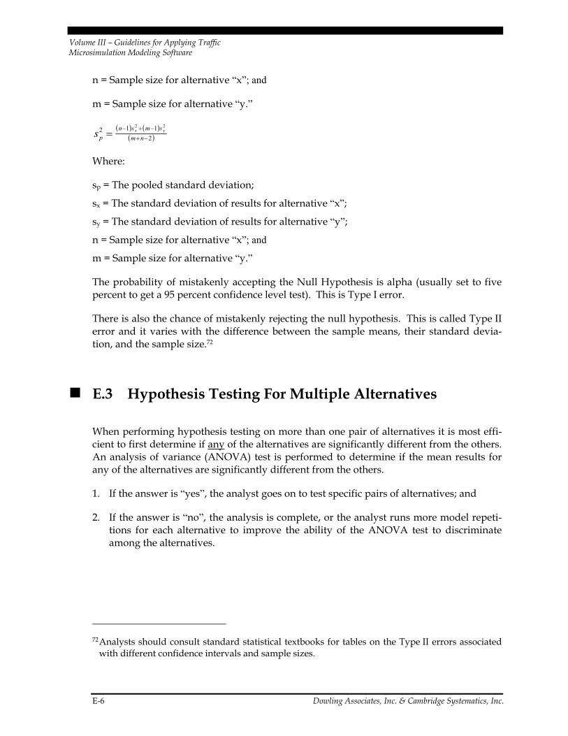
Volume III – Guidelines for Applying Traffic Microsimulation Modeling Software
E-6 Dowling Associates, Inc. & Cambridge Systematics, Inc.
n = Sample size for alternative “x”; and
m = Sample size for alternative “y.”
( ) ( )( )2
11222
−+−+−= nm
smsnp
yxs
Where:
sp = The pooled standard deviation;
sx = The standard deviation of results for alternative “x”;
sy = The standard deviation of results for alternative “y”;
n = Sample size for alternative “x”; and
m = Sample size for alternative “y.”
The probability of mistakenly accepting the Null Hypothesis is alpha (usually set to five percent to get a 95 percent confidence level test). This is Type I error.
There is also the chance of mistakenly rejecting the null hypothesis. This is called Type II error and it varies with the difference between the sample means, their standard devia-tion, and the sample size.72
E.3 Hypothesis Testing For Multiple Alternatives
When performing hypothesis testing on more than one pair of alternatives it is most effi-cient to first determine if any of the alternatives are significantly different from the others. An analysis of variance (ANOVA) test is performed to determine if the mean results for any of the alternatives are significantly different from the others.
1. If the answer is “yes”, the analyst goes on to test specific pairs of alternatives; and
2. If the answer is “no”, the analysis is complete, or the analyst runs more model repeti-tions for each alternative to improve the ability of the ANOVA test to discriminate among the alternatives.
72 Analysts should consult standard statistical textbooks for tables on the Type II errors associated
with different confidence intervals and sample sizes.

Volume III – Guidelines for Applying Traffic Microsimulation Modeling Software
Dowling Associates, Inc. & Cambridge Systematics, Inc. E-7
E.3.1 Analysis of Variance (ANOVA) Test
ANOVA has three basic requirements:
1. Independence of Samples (random samples);
2. Sampling distribution of means is normal; and
3. Equal variances of groups.
Levine’s test of heteroscedasticity can be used for testing whether or not the variances of model run results for each alternative are similar. Less powerful non-parametric tests, such as Kruskal-Wallis test (K-W Statistic) can be performed if the requirements of ANOVA cannot be met.
However, ANOVA is tolerant of modest violations of these requirements, and may still be a useful test under these conditions. ANOVA will tend to be conservative if its require-ments are not completely met (less likely to have Type I error with a lower power of the test to correctly reject the null hypothesis).
To perform the ANOVA test first compute the test statistic:
MSWMSBF =
Where:
F = The test statistic
MSB = The mean square error between alternatives (formula provided below)
MSW = The mean square error among model results for the same alternative (within alternatives)
The formulae below show how to compute MSB and MSW.
1
)(1
2
−
−•=∑=
g
xxnMSB
g
iii
Where:
MSB = Mean square error between alternatives (i = 1 to g);
ni = Number of model runs with different random number seeds for alternative “i”;
=ix The mean value for alternative “i”;
=x The mean value averaged across all alternatives and runs; and
g = The number of alternatives.

Volume III – Guidelines for Applying Traffic Microsimulation Modeling Software
E-8 Dowling Associates, Inc. & Cambridge Systematics, Inc.
and:
gN
snMSW
g
iii
−
•−=∑=1
2)1(
Where:
MSB = Mean square error between alternatives (i=1 to g);
ni = Number of model runs with different random number seeds for alternative “i”;
=2is The variance of the model run results for alternative “i”;
N = The total number of model runs summed over all alternatives; and
g = The number of alternatives.
The null hypothesis of equal means is rejected if:
F > F1-alpha,g-1,N-g
Where:
F1-alpha,g-1,N-g = The “F” statistic for a Type I error of “alpha” (alpha is usually set at five per-cent for a 95 percent confidence level) and g-1 and N-g degrees of freedom. N is the total number of model runs summed over all alternatives. “g” is the number of alternatives.
If the null hypothesis cannot be rejected, then the analysis is either done (there is no sta-tistically significant difference between any of the alternatives at the 95 percent confidence level) or the analyst should consider reducing the level of confidence to below 95 percent or implementing more model runs per alternative to improve the sensitivity of the ANOVA test.
E.3.2 Pairwise Tests of Some Pairs of Alternatives
If performing hypothesis tests for only a few of the potential pairs of alternatives, the standard “t” test can be used for comparing a single pair of alternatives.
mnpmn styx 11)2();2/1( +•>− −+−α
=− yx The absolute value of the difference in the mean results for alternative “x” and alternative “y”;
sp = The pooled standard deviation;
t = The “t” distribution for a level of confidence of (1-alpha) and (n+m-2) degrees of freedom;
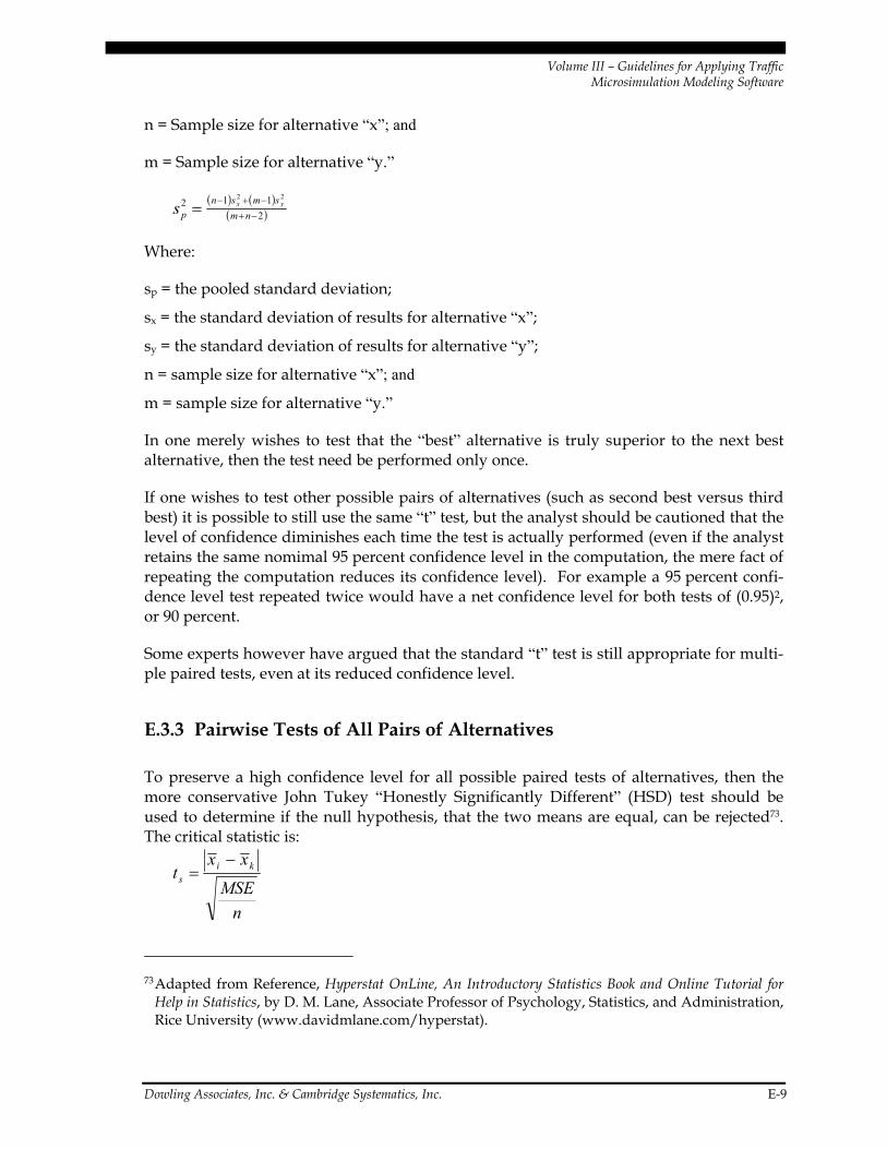
Volume III – Guidelines for Applying Traffic Microsimulation Modeling Software
Dowling Associates, Inc. & Cambridge Systematics, Inc. E-9
n = Sample size for alternative “x”; and
m = Sample size for alternative “y.”
( ) ( )( )2
11222
−+−+−= nm
smsnp
yxs
Where:
sp = the pooled standard deviation;
sx = the standard deviation of results for alternative “x”;
sy = the standard deviation of results for alternative “y”;
n = sample size for alternative “x”; and
m = sample size for alternative “y.”
In one merely wishes to test that the “best” alternative is truly superior to the next best alternative, then the test need be performed only once.
If one wishes to test other possible pairs of alternatives (such as second best versus third best) it is possible to still use the same “t” test, but the analyst should be cautioned that the level of confidence diminishes each time the test is actually performed (even if the analyst retains the same nomimal 95 percent confidence level in the computation, the mere fact of repeating the computation reduces its confidence level). For example a 95 percent confi-dence level test repeated twice would have a net confidence level for both tests of (0.95)2, or 90 percent.
Some experts however have argued that the standard “t” test is still appropriate for multi-ple paired tests, even at its reduced confidence level.
E.3.3 Pairwise Tests of All Pairs of Alternatives
To preserve a high confidence level for all possible paired tests of alternatives, then the more conservative John Tukey “Honestly Significantly Different” (HSD) test should be used to determine if the null hypothesis, that the two means are equal, can be rejected73. The critical statistic is:
nMSE
xxt ki
s
−=
73 Adapted from Reference, Hyperstat OnLine, An Introductory Statistics Book and Online Tutorial for
Help in Statistics, by D. M. Lane, Associate Professor of Psychology, Statistics, and Administration, Rice University (www.davidmlane.com/hyperstat).

Volume III – Guidelines for Applying Traffic Microsimulation Modeling Software
E-10 Dowling Associates, Inc. & Cambridge Systematics, Inc.
Where:
ts = The studentized “t” statistic;
=ix The mean value for alternative “i”;
MSE = The mean square error = MSB + MSW; and
N = the number of model runs with different random number seeds for each alternative (If the number of runs for each alternative is different then use the harmonic mean of the number of runs for each alternative.).
Reject the null hypothesis that the mean result for alternative “i” is equal to that for alter-native “k” if:
ts > t1-alpha, g-1
Where:
t1-alpha, g-1 = The “t” statistic for a desired Type I error of “alpha” (alpha is usually set at five percent to obtain a 95 percent confidence level) and “g-1” degrees of freedom, with “g” equal to the total number of alternatives tested, not just the two being compared in each test.
Some experts consider the HSD test to be too conservative, failing to reject the null hypothesis of equal means when it should be rejected. The price of retaining a high confi-dence level (same as retaining a low probability of a Type I error) is a significantly increased probability of making a Type II error (accepting the null hypothesis when it is really false).
E.4 What To Do if the Null Hypothesis Cannot Be Rejected
If the null hypothesis of no significant difference in the mean results for the alternatives cannot be rejected, then the analyst has the following options:
1. Increase the number of model run repetitions per alternative until the simulation per-formance of one alternative can be distinguished from the other.
2. Reduce the confidence level from 95 percent to a lower level where the two alterna-tives are significantly different, and report the lower confidence level in the results.
3. Accept the results that the two alternatives are not significantly different.

Volume III – Guidelines for Applying Traffic Microsimulation Modeling Software
Dowling Associates, Inc. & Cambridge Systematics, Inc. F-1
Appendix F. Demand Constraint
Microsimulation results are highly sensitive to the amount by which the demand exceeds the capacity of the facility, so it is vital that realistic demand forecasts be used in the analysis. The following steps outline a procedure for manually reducing the forecasted demands in the study area to better match the capacity of the facilities feeding the study area.
Step 1. Identify Gateway Bottlenecks
The analyst should first identify the critical bottlenecks on the facilities feeding the traffic to the boundaries of the microsimulation study area. Bottlenecks are sections of the facili-ties feeding the model study area that either have capacities less than other sections of the freeway or demands greater than the other sections. These are the locations likely to be the first ones to experience congested conditions as traffic grows.
These bottlenecks may be located on the boundary of the microsimulation study area, in which case they are identical to the gateway zones on the boundary of the microsimula-tion model study area. Bottlenecks within the microsimulation model study area can be disregard, since they will be taken into account by the microsimulation model.
Inbound bottlenecks are congested sections feeding traffic to the microsimulation model area. Outbound bottlenecks are congested sections affecting traffic leaving the microsimulation model area. If an outbound bottleneck is likely to create future queues that back up into the microsimulation model study area, then the model study area should be extended outwards to include the outbound bottleneck. If the future outbound queues will not back up into the model study area then these bottlenecks can be safely disregarded.

Volume III – Guidelines for Applying Traffic Microsimulation Modeling Software
F-2 Dowling Associates, Inc. & Cambridge Systematics, Inc.
Figure F.1 Bottleneck, Gateway, and Study Area
MicrosimulationModel Study Area
Bottleneck
Gateway
Step 2. Estimate Excess Demand at Inbound Bottlenecks
If the forecasted hourly demand at a bottleneck (in the inbound direction to the model) exceeds its capacity, the proportion of the demand that is in excess of the available hourly capacity should be computed.
CCDX −
=
Where:
X = Proportion of excess demand;
D = Forecasted demand (vehicles per hour); and
C = Estimated capacity (vehicles per hour).
Step 3. Reduce Forecasted Demand Inbound at Gateways
The forecasted hourly demands for the off-ramps between the bottleneck and the gateway entering the microsimulation study area should be reduced in proportion to the amount by which the forecasted bottleneck demand exceeds its capacity.
)1(* XDD unconstconst −=
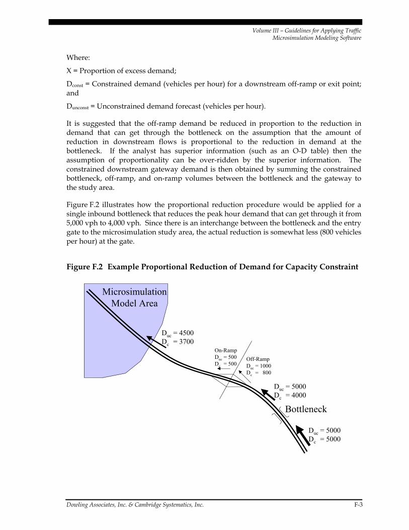
Volume III – Guidelines for Applying Traffic Microsimulation Modeling Software
Dowling Associates, Inc. & Cambridge Systematics, Inc. F-3
Where:
X = Proportion of excess demand;
Dconst = Constrained demand (vehicles per hour) for a downstream off-ramp or exit point; and
Dunconst = Unconstrained demand forecast (vehicles per hour).
It is suggested that the off-ramp demand be reduced in proportion to the reduction in demand that can get through the bottleneck on the assumption that the amount of reduction in downstream flows is proportional to the reduction in demand at the bottleneck. If the analyst has superior information (such as an O-D table) then the assumption of proportionality can be over-ridden by the superior information. The constrained downstream gateway demand is then obtained by summing the constrained bottleneck, off-ramp, and on-ramp volumes between the bottleneck and the gateway to the study area.
Figure F.2 illustrates how the proportional reduction procedure would be applied for a single inbound bottleneck that reduces the peak hour demand that can get through it from 5,000 vph to 4,000 vph. Since there is an interchange between the bottleneck and the entry gate to the microsimulation study area, the actual reduction is somewhat less (800 vehicles per hour) at the gate.
Figure F.2 Example Proportional Reduction of Demand for Capacity Constraint
MicrosimulationModel Area
Bottleneck
Duc = 5000Dc = 4000
Duc = 5000Dc = 5000
Off-RampDuc = 1000Dc = 800
On-RampDuc = 500Dc = 500
Duc = 4500Dc = 3700

Volume III – Guidelines for Applying Traffic Microsimulation Modeling Software
F-4 Dowling Associates, Inc. & Cambridge Systematics, Inc.
Starting upstream of the bottleneck there is an unconstrained demand for 5,000 vph. Since the bottleneck has a capacity of 4,000 vph, the downstream capacity constrained demand is reduced from the unconstrained level of 5,000 vph to 4,000 vph. Thus, 1000 vehicles are stored at the bottleneck during the peak hour. Since it is assumed that the stored vehicles are destined to downstream destinations in proportion to the exiting volumes at each off-ramp and freeway mainline, the downstream volumes are reduced the same percentage as the percentage reduction at the bottleneck (20 percent). A 20 percent reduction of the off-ramp volume results in a constrained demand of 800 vehicles per hour. The on-ramp volume is unaffected by the upstream bottleneck, so its unconstrained demand is unchanged at 500 vph. The demand that enters the microsimulation study area is equal to the constrained demand of 4,000 vph leaving the bottleneck, minus the 800 vph leaving the freeway on the off-ramp, plus 500 entering the freeway at the onramp which results in a constrained demand of 3,700 vph.

Volume III – Guidelines for Applying Traffic Microsimulation Modeling Software
Dowling Associates, Inc. & Cambridge Systematics, Inc. G-1
Appendix G. References
G.1 Traffic Microsimulation Fundamentals
1. Revised Monograph on Traffic Flow Theory, N. H. Gartner, C. J. Messer, A. Ruthi (editors), Federal Highway Administration, 1994 (available at: http://www.tfhrc.gov/its/tft).
2. May, A. D., Traffic Flow Fundamentals, Prentice Hall, Englewood Cliffs, New Jersey, 1990.
3. Ahmed, K. I., Modeling Drivers’ Acceleration and Lane Changing Behavior, Ph.D. Dissertation, Massachusetts Institute of Technology, Cambridge, Massachusetts, February 1999.
4. Elefteriadou, L., G. List, J. Leonard, H. Lieu, M. Thomas, R. Giguere, R. Brewish, G. Johnson, Beyond the Highway Capacity Manual: A Framework for Selecting Simulation Models in Traffic Operational Analyses, Transportation Research Record 1678, National Academy Press, 1999, pp. 96-106.
G.2 Calibration and Validation of Microsimulation Models
5. Abdullai, B., J. Sheu, W. Recker, Simulation of ITS on the Irvine FOT Area Using ‘Paramics 1.5’ Scalable Microscopic Traffic Simulator: Phase I: Model Calibration and Validation, California PATH Program Research Report (UCB-ITS-PRR-99-12), University of California, Berkeley, 1999.
6. Ben-Akiva, M., A. Davol, T. Toledo, H. N. Koutsopoulos, W. Burghout, I. Andréasson, T. Johansson, C. Lundin, Calibration and Evaluation of MITSIMLab in Stockholm, Paper presented at Annual Meeting, Transportation Research Board, Washington, D.C., 2002.
7. Fellendorf, M., P. Vortisch, Validation of the Microscopic Traffic Flow Model VISSIM in Different Real-World Situations, Paper presented at Annual Meeting, Transportation Research Board, Washington, D.C., 2001 (also available from http://www.itc-world.com/library).
Volume III – Guidelines for Applying Traffic Microsimulation Modeling Software
G-2 Dowling Associates, Inc. & Cambridge Systematics, Inc.
8. Freeway System Operational Assessment, Technical Report I-33, Paramics Calibration and Validation Guidelines, Draft, Wisconsin DOT, District 2, Milwaukee, Wisconsin, June 2002.
9. Gardes, Y., A. D. May, J. Dahlgren, A. Skabardonis, Bay Area Simulation and Ramp Metering, California PATH Research Report.
10. Hellinga, B. R., Requirements for the Calibration of Traffic Simulation Models, Canadian Society of Civil Engineering (CSCE), University of Waterloo, 1998.
11. Jayakrishnan, R., J. Oh, A. B. Sahraoui, Calibration and Path Dynamics Issues in Microscopic Simulation for Advanced Traffic Management and Information Systems, UCI-ITS-WP-00-22, Institute of Transportation Studies, University of California, Irvine, California, December 2000
12. Lee, D-H., X. Yang, P. Chandrasekar, Parameter Calibration for PARAMICS Using Genetic Algorithm, Paper Number 01-2339, Annual Meeting, Transportation Research Board, Washington, D.C., 2001.
13. Ma, T., B. Abdulhai, A Genetic Algorithm-Based Optimization Approach and Generic Tool for the Calibration of Traffic Microscopic Simulation Parameters, Paper presented at Annual Meeting, Transportation Research Board, Washington, D.C., 2002.
14. Owen, L. E., G. Brock, S. Mastbrook, R. Pavlik, L. Rao, C. Stallard, S. Sunkari, Y. Zhang, A Compendium of Traffic Model Validation Documentation and Recommendations, DTFH61-95-C-00125, Federal Highway Administration, Washington, D.C., 1995.
15. Project Suite Calibration and Validation Procedures, Quadstone, Ltd., Edinburgh, United Kingdom, February 2000 (http://www.paramics-online.com/tech_support/ customer/cust_doc.htm password required).
16. Rakha, H., B. Hellinga, M. Van Aerde, and W. Perez, Systematic Verification, Validation and Calibration of Traffic Simulation Models, Annual Meeting, Transportation Research Board, Washington, D.C., 1996.
17. Rao, L., L. Owen, D. Goldsman, Development and Application of a Validation Framework for Traffic Simulation Models, Proceedings of the 1998 Winter Simulation Conference; D. J. Medeiros, E. F. Watson, J. S. Carson, and M. S. Manivannan (editors).
18. Skabardonis, A., Simulation of Freeway Weaving Areas, Preprint No. 02-3732, Annual Meeting, Transportation Research Board, Washington, D.C., 2002.
19. Traffic Appraisal in Urban Areas: Highways Agency, Manual for Roads and Bridges, Volume 12, Department for Transport, London, May 1996, (http://www.archive.official-documents.co.uk/document/ha/dmrb/index.htm).
Volume III – Guidelines for Applying Traffic Microsimulation Modeling Software
Dowling Associates, Inc. & Cambridge Systematics, Inc. G-3
20. Wall, Z., R. Sanchez, and D. J. Dailey, A General Automata Calibrated with Roadway Data for Traffic Prediction, Paper No. 01-3034, Annual Meeting, Transportation Research Board, Washington, D.C., 2001.
G.3 Analysis of Results
21. Benekohal, R. F., Y. M. Elzohairy, J. E. Saak, A Comparison of Delay from HCS, Synchro, Passer II, Passer IV, and CORSIM for an Urban Arterial, Preprint, Annual Meeting, Transportation Research Board, Washington, D.C., 2002.
22. Joshi, S. S., A. K. Rathi, Statistical Analysis and Validation of Multi-population Traffic Simulation Experiments, Transportation Research Record 1510, Transportation Research Board, Washington, D.C., 1995.
23. Prassas, E. S., A Comparison of Delay on Arterials by Simulation and HCM Computations, Preprint No. 02-2652, Annual Meeting, Transportation Research Board, Washington, D.C., 2002.
24. Tian, Z. Z., T. Urbanik II, R. Engelbrecht, K. Balke, Variations in Capacity and Delay Estimates from Microscopic Traffic Simulation Models, Preprint, Annual Meeting, Transportation Research Board, Washington, D.C., 2002.
25. Trueblood, M., CORSIM..Simtraffic: What’s the Difference?, PCTRANS, Winter/Spring 2001.
26. Gibra, I. N., Probability and Statistical Inference for Scientists and Engineers, Prentice-Hall, Englewood Cliffs, New Jersey, 1973.
27. Lane, D. M., Hyperstat OnLine, An Introductory Statistics Book and Online Tutorial for Help in Statistics, Rice University (www.davidmlane.com/hyperstat).
28. Gerstman, B., and M. Innovera, StatPrimer Version 5.1, California State University, San Jose, (http://www.sjsu.edu/faculty/gerstman/StatPrimer/).