volume vi - berkeley economic review · volume vi 9 1st place winner brandon deutscsh class of 2020...
TRANSCRIPT

VOLUME VI
BERKELEY ECONOMIC REVIEW
TABLE OF CONTENTSESSAY CONTEST
Let's Actually Invest in Our Students ..................... 9Brandon Deutsch
We Need Alternatives to Student Loans; Not More University Subsidies ..................................................... 10Elliot Witter
The Underlying Accountability Problem Behind Rising Tuition ........................................................ 11Gamin Kim
INTERVIEW ............................................................ 12
RESEARCH PAPERS
Time Discipline and Southern Railroads Increased Watch Availability Raising Labor Costs ............... 16David Abraham, University of Chicago
The Sino-African Relationship: An Empirical Study of the Effect of Chinese Foreign Direct Investment on Illicit Financial Flows in Africa ........................ 56Fatima Ezzahra Daif, Yale-NUS College
Real Exchange Rate Volatility and Economic Growth: A Panel Data Investigation .................... 98Federico Pessina, University of Warwick
VOLUME VI
PEER REVIEW BOARD
SUBMISSIONS POLICYFormat: Please format your submission as a Microsoft word document or Latex file. We would prefer submissions single-spaced in size 12, Times New Roman font. Length: Maximum five pages single-spaced for essays or op-eds, not including works cited page(s). No maximum for theses or original research papers.Plagiarism: We maintain a strict zero tolerance policy on plagiarism. According to the University of North Carolina, plagiarism is “the deliberate or reckless representation of another’s words, thoughts, or ideas as one’s own without attribution in connection with submission of academic work, whether graded or otherwise.” For more information about plagiarism – what it is, its consequences, and how to avoid it – please see the UNC’s website.Citations: Use MLA format for in-text citations and your works cited page. Include a separate works cited page at the end of your work.Send to: [email protected]
DISCLAIMERThe views published in this journal are those of the individual writers or speakers and do not necessarily reflect the position or policy of Berkeley Economic Review or the University of California at Berkeley.
COPYRIGHT POLICY All authors retain copyright over their original work. No part of our journal, whether text or image, may be used for any purpose other than personal use. For permission to reproduce, modify, or copy materials printed in this journal for anything other than personal use, kindly contact the respective authors.
Alina SkripetsAmmar Inayatali
Angel HsuArthur Chen
Margaret ChenRenata Carreiro Avila
Simon ZhuTommy lao
(IN ALPHABETICAL ORDER)

BERKELEY ECONOMIC REVIEW
4
STAFF
Margaret ChenManaging Editor
Peer Review*
Joseph HernandezManaging Editor
Anastasia PyrinisResearch & Editorial*
Charles McMurryMarketing*Webmaster
Juliana ZhaoMarketing*
Katherine ShengLayout & Design*
Simon ZhuResearch & Editorial*
Peer Reviewer
Vatsal BajajProfessional
Development*
Vinay MaruriProfessional
Development*
Alex ChengAssistant Editor
Ammar InayataliPeer Reviewer
Angel HsuPeer Reviewer
Antara JhaProfessional
Development Associate
Ariana JessaStaff Writer- Qualitative
Arsh VishenStaff Writer
- Quantitative
Avik SethiaProfessional
Development Associate
Dana WuAssistant Editor
Colleen GabrimassihiMarketing Associate

VOLUME VI
5
STAFF
Devesh AgarwalProfessional
Development Associate
Gurmehar Kaur SomalMarketing Associate
Joseph NgStaff Writer- Qualitative
Krunal DesaiProfessional
Development Associate
Matthew McBrideAssistant EditorLayout Editor
Parmita DasStaff Writer- Qualitative
Reilly OlsonMarketing Associate
Renata Carreiro AvilaPeer Reviewer
Selena ZhangMarketing Associate
Seth BertolucciStaff Writer
- Quantitative
Sofia GuoAssistant Editor
Tommy laoPeer Review Editor
Vassilisa RubtsovaStaff Writer
- Qualitative
Melika RahbarLayout Editor
Danny ChandrahasanLayout Editor
* Department Heads
Shreyas HariharanMarketing Associate
Yechan ShinAssistant Editor
BERKELEY ECONOMIC REVIEW
6
STAFF
• Alessandro Ortenblad, Assistant Editor •
• Alina Skripets, Contributor •
• Arthur Chen, Peer Reviewer •
• Jacob Fajnor, Contributor •
• Jaeun Park, Layout Editor •
• Kailin Li, Layout Editor •
• Katherine Blesie, Staff Writer - Qualitative •
• Odysseus Pyrinis, Staff Writer - Qualitative •
• Rachel Hobbs, Contributor •
• Renuka Garg, Assistant Editor •
• Rishi Modi, Marketing Associate •
• Sasyak Pattnaik, Contributor •
• Sergio Andre C. Nascimento, Contributor •
Additional Staff Not Pictured:

VOLUME VI
7
[THIS PAGE INTENTIONALLY LEFT BLANK]

Fall 2018 Essay Contest
Rising tuition and student loans have become a pressing issue in the United States.
Should tuition to public universities be partially subsidized, completely
subsidized, left in their current state, or otherwise altered?
VOLUME VI
9
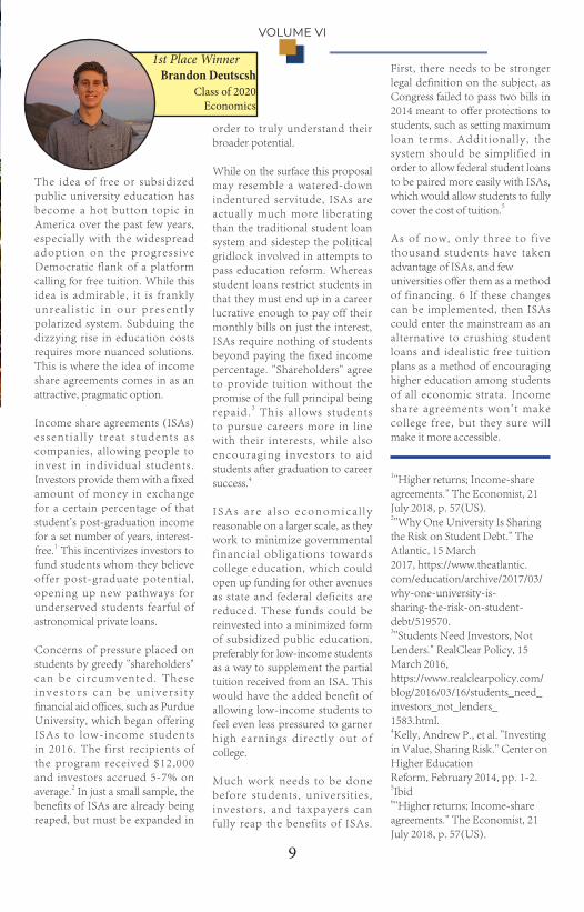
1st Place Winner Brandon Deutscsh
Class of 2020 Economics
The idea of free or subsidized public university education has become a hot button topic in America over the past few years, especially with the widespread adopt ion on the progress ive Democratic flank of a platform calling for free tuition. While this idea is admirable, it is frankly u n r e a l i s t i c i n o u r p r e s e n t l y polarized system. Subduing the dizzying rise in education costs requires more nuanced solutions. This is where the idea of income share agreements comes in as an attractive, pragmatic option.
Income share agreements (ISAs) e s s e n t i a l l y t r e a t s t u d e n t s a s companies, allowing people to invest in individual students. Investors provide them with a fixed amount of money in exchange for a certain percentage of that student's post-graduation income for a set number of years, interest-free.1 This incentivizes investors to fund students whom they believe offer post-graduate potential, opening up new pathways for underserved students fearful of astronomical private loans.
Concerns of pressure placed on students by greedy "shareholders" can be c i rcumvented. These i n v e s t o r s c a n b e u n i v e r s i t y financial aid offices, such as Purdue University, which began offering ISAs to low-income students in 2016. The first recipients of the program received $12,000 and investors accrued 5-7% on average.2 In just a small sample, the benefits of ISAs are already being reaped, but must be expanded in
First, there needs to be stronger legal definition on the subject, as Congress failed to pass two bills in 2014 meant to offer protections to students, such as setting maximum loan terms. Additionally, the system should be simplified in order to allow federal student loans to be paired more easily with ISAs, which would allow students to fully cover the cost of tuition.5
As of now, only three to f ive thousand students have taken advantage of ISAs, and fewuniversities offer them as a method of financing. 6 If these changes can be implemented, then ISAs could enter the mainstream as an alternative to crushing student loans and idealistic free tuition plans as a method of encouraging higher education among students of all economic strata. Income share agreements won't make college free, but they sure will make it more accessible.
1"Higher returns; Income-share agreements." The Economist, 21 July 2018, p. 57(US).2"Why One University Is Sharing the Risk on Student Debt." The Atlantic, 15 March2017, https://www.theatlantic.com/education/archive/2017/03/why-one-university-is-sharing-the-risk-on-student-debt/519570.3"Students Need Investors, Not Lenders." RealClear Policy, 15 March 2016,https://www.realclearpolicy.com/blog/2016/03/16/students_need_investors_not_lenders_1583.html.4Kelly, Andrew P., et al. "Investing in Value, Sharing Risk." Center on Higher EducationReform, February 2014, pp. 1-2.5Ibid6"Higher returns; Income-share agreements." The Economist, 21 July 2018, p. 57(US).
order to truly understand their broader potential.
While on the surface this proposal may resemble a watered-down indentured servitude, ISAs are actually much more liberating than the traditional student loan system and sidestep the political gridlock involved in attempts to pass education reform. Whereas student loans restrict students in that they must end up in a career lucrative enough to pay off their monthly bills on just the interest, ISAs require nothing of students beyond paying the fixed income percentage. "Shareholders" agree to provide tuition without the promise of the full principal being repaid. 3 This a l lows students to pursue careers more in line with their interests, while also encouraging investors to aid students after graduation to career success.4
I S A s a r e a l s o e c o n o m i c a l l y reasonable on a larger scale, as they work to minimize governmental f inancial obligations towards college education, which could open up funding for other avenues as state and federal deficits are reduced. These funds could be reinvested into a minimized form of subsidized public education, preferably for low-income students as a way to supplement the partial tuition received from an ISA. This would have the added benefit of allowing low-income students to feel even less pressured to garner high earnings direct ly out of college.
Much work needs to be done before students, universit ies, investors , and taxpayers can fully reap the benefits of ISAs.

BERKELEY ECONOMIC REVIEW
10
2nd Place Winner Elliot Witter Class of 2019
Business Administration
Within the next decade, we could live in a world where ISAs are securitized products allowing private and public investors to fund education while generating stable returns. Just as corporate b o n d s f u e l t h e g r o w t h o f innovative companies like Netflix and Tesla, so too could securitized ISAs fuel the growth of educational achievement. Better still, ISAs offer a healthy alternative to student loans because they are less rigid on borrowers and impose no additional costs to taxpayers.
• Cooper, Preston. “How Tax Reform Affected These Hidden Subsidies for Higher Education”.Forbes. May 30, 2018. https://www.forbes.com/sites/prestoncoo-per2/2018/05/30/how-tax-reform-affected-these-hid-den-subsidies-for-higher-educa-tion/#1414be833956.• “Trends in Higher Education”. Col-legeBoard. Accessed October 20, 2018.https://trends.collegeboard.org/student-aid/figures-tables/pell-grants-total-expenditures-max-imum-and-average-grant-and-num-ber-recipients-over-time.• “Income-share agreements are a novel way to pay tuition fees”. The Economist. July 19, 2018. https://www.economist.com/finance-and-eco-nomics/2018/07/19/income-share-agreements-are-a-novel-way-to-pay-tuition-fees?frsc=dg%7Ce.• Marcus, Jon. “How free college tui-tion in one country exposes unexpect-ed pros and cons”. TheHechinger Report. October 18, 2016. https://hechingerreport.org/free-col-lege-tuition-one-country-exposes-unexpect-ed-pros-cons/.• Wirtz, Bill. “France Shows That ‘Free’ College is Neither Free Nor Fair”. Foundation for Economic Education. October 3, 2016. https://fee.org/arti-cles/france-shows-that-free-college-is-neither-free-nor-fair/.• “Higher Education”. California En-acted 2018-19 State Budget. Accessed October 20, 2018.http://www.ebudget.ca.gov/2018-19/pdf/Enacted/BudgetSummary/High-erEducation.pdf.
tuition has decreased the efficiency of their education system.
If free tuition is not the solution to providing abundant education, then what is? One idea comes to mind: rather than increasing subsidies, we should focus on of fer ing addi t iona l ways for i n d i v i d u a l s t o f i n a n c e t h e i r education.
The federal government already offers student loans at below-market rates, but their repayment terms are inflexible during poor economic times and for lower-e a r n i n g b o r r o w e r s . A m o r e effective financing method would be what are dubbed Income Share Agreements, or ISAs, whereby college students receive a loan in exchange for a percentage of their earnings for a predetermined number of years after graduation. Unlike loans, which require fixed interest and principal payments r e g a r d l e s s o f e m p l o y m e n t , ISA repayments adjust to what graduates can afford. They also cannot l inger indefinitely, as student loans frequently do.
ISAs are already being put into practice. For example, Purdue U n i v e r s i t y l a u n c h e d a n I S A program in 2016 using funds from their endowment. So far, the program has seen the average ISA cover $12,000 in fees while generating 5-7% returns. This return aspect is the most important factor in determining a widespread rollout of ISAs. If it is proven that returns are stable, and high enough given the current interest rate environment, private investors will want a piece of the market. Once private capital is involved, ISAs could begin expansion to millions of students across the country.
Abundant access to education, including universities, is essential for a functioning democracy and vibrant economy. While our state governments furnish us with completely subsidized primary and secondary schooling, the same should not be said for public universities.
To c lar i fy , f edera l and s ta te governments already spend billions each year to lower university tuition costs. For example, the federal government spent $28 billion in the 2017-18 fiscal year on Pe l l Grants for 7 mi l l ion students, and another $47 billion on tuition tax credits, charitable deductions for education, and o t h e r e d u c a t i o n - r e l a t e d t a x benefits. State expenditures are even greater. California subsidies for UC students have increased 26% since 2011-12 to $12,098 per full-time equivalent student. The fact that tuitions are still high tells us that receiving a high-quality university education is expensive, and therefore its pursuit should be viewed as a calculated investment for any aspiring undergraduate.
It is true that higher education has more to offer than just financial benefits. Before jumping to the conclusion that we need "free" tuition, one should first look at European countries that have already made that decision. As an example, when Germany decided to completely subsidize university education in 2014, enrollment i n c r e a s e d 2 2 % . M e a n w h i l e , education subsidy costs increased 37% and spending per student declined by 10%, albeit over several years. Clearly, the move to free
VOLUME VI
11
3rd Place Winner Gamin Kim Class of 2022
Political Science
Since the post-WWII era, the United States has championed itself as the leader in higher education and the provider of intellectual and career-driven opportunities in the world. The passage of legislation such as the G.I. Bill and the Higher Education Act of 1965 propelled the belief of the indispensable qual i ty of col lege education. T h r o u g h f e d e r a l s u b s i d i e s , scholarships, and low-interest loans, the government enabled veterans and individuals from low-income households alike to follow various employment pathways. Essentially, direct entrance into the job market was no longer the only permissible recourse.
The hopeful and lighthearted narrative of higher education in modernity has been remarkably dismantled due to rising costs of tuition and the strained burden of student loans. For the past 30 years, the average published tuition and fees for a public four-year college increased by 6,780 dollars.1 Furthermore, the increase in college tuition has lowered the attraction of higher education, with aggregate college enrollment falling for the past five years;2 the value and the benefits tied with attending college has developed into interests worth questioning and rethinking for the sake of financial stability. Despite the enticing nature of federal higher education subsidies, such as student loans and the Pell Grant, partial or complete tuition subsidization to public universities now will only worsen the existing acute levels of price inflation. Rather than attempt to resolve
past 40 years, so much so that it has lost its original intention and basis. To truly progress student loan and tax benefits to favor both students and the American worker, federal policies ought to be simplified and more targeted towards students of low-income households.7 This way, the subsidies will benefit those who are in actual need of them.
1Ma, Jennifer, Sandy Baum, Matea Pender, and CJ Libassi, Trends in Col-lege Pricing 2018 (New York: The Col-lege Board, 2018), https://trends.col-legeboard.org/sites/default/files/2018-trends-in-college-pricing.pdf.2CCAP, “Seven Challenges Facing Higher Education,” Forbes Maga-zine, August 29, 2017, https://www.forbes.com/sites/ccap/2017/08/29/seven-challenges-facing-higher-edu-cation/.3Josh Mitchell, “Federal Aid’s Role in Driving Up Tuitions Gains Credence,” Wall Street Journal, August 2, 2015, https://www.wsj.com/articles/federal-aids-role-in-driving-up-tuitions-gains-credence-1438538582.4David O. Lucca, Taylor Nadauld, Karen Shen, Credit Supply and the Rise in College Tuition: Evidence from the Expansion in Federal Student Aid Programs (New York: Federal Reserve Bank of New York, 2015), https://www.newyorkfed.org/medialibrary/media/research/staff_reports/sr733.pdf.5Tim Worstall, “Increased Tuition Sub-sidies Increase The Price of College Tuition,” Forbes Magazine, August 3,2015, https://www.forbes.com/sites/timworstall/2015/08/03/increased-tuition-subsidies-in-crease-the-price-of-college-tuitio n/#2fb9e36345a2.6Adam Davidson, “Is College Tuition Really Too High?” New York Times, September 8, 2015, https://www.nytimes.com/2015/09/13/magazine/is-college-tuition-too-high.html.7Elaine Maag, David Mundel, Lois Rice, and Kim Rueben, “Subsidizing Higher Education through Tax and Spending Programs” (Washington, DC: Urban-Brookings Tax Policy Center, 2007), https://www.brookings.edu/wp-content/uploads/2016/06/lrice200705.pdf.
the central concern in higher education through subsidization alone, greater accountabi l i ty towards educational institutions and the system of financial aid disbursement in this country needs to be held before any subsequent financial policies take into effect.
The New York Federal Reserve in 2015 explicit ly faulted the policies of the federal government to establish the concept of an affordable college, for the aid growth has only empowered e d u c a t i o n a l i n s t i t u t i o n s t o egregiously hike tuit ion up.3 Student loans, di f ferences in student borrowing, and tuition are all intertwined; if one is modified, i t tr iggers change and affects the other two as well . Simply put, institutions that were more exposed to modifications in the subsidized federal loan program increased their tuit ion about 65 percent because of federal action.4 The rise in tuition and federal aid boosts is linked to disparate economic implications. The sequence between inflation and more extensive government support can eventually impact taxpayers negatively and prevent s o m e i n d i v i d u a l s t o a t t e n d higher education, a pattern some economists are comparing to the late 2000's housing bubble.5
Col lege aid has evolved into a system that awards students from middle-class and affluent h o u s e h o l d s w h o a t t e n d p r i v a t e n o n p r o f i t c o l l e g e s disproportionately more than those disadvantaged who go to public community colleges.6 The role of higher education policy in the federal government has transformed dramatically over the

BERKELEY ECONOMIC REVIEW
12
ProfessorDMITRY
TAUBINSKY
Interviewer: Joseph NgPhotographer: Aislin Liu

VOLUME VI
13
Interviewer: Could you being by telling me a little bit about your background, how you got involved with economics?
Prof. Taubinsky: I actually started out as a math major in college, but I always wanted to do something that’s more in the real world. I was always interested in psychology, and I generally just enjoyed the so-cial sciences, so economics seemed like it would allow me to com-bine my interest in math with my interest in the real world. Early on I contacted David Laibson, who is a behavioral economist at Harvard, and I got very lucky and got a chance to work in his group as a research assistant starting the summer after my freshman year. Getting a taste for research early on is what really pulled me into economics. I spent the rest of my summers in college working on research in David’s group, and every summer I just got more and more excited about economics. So it was very clear for me that I wanted to go to graduate school and do something in the area of behavioral economics.
Interviewer: I read one of your working papers on the soda tax, and it was really interesting because it introduced the topic in a way that I hadn’t necessarily thought about before, how some of the benefits are also regressive, impacting lower income, lower socio-economic status members of society. What, may I ask, inspired that paper, that direction of research, for you?
Prof. Taubinsky: A lot of it is real world relevance. It’s a new kind of tax that more and more cities are considering, and it’s clearly a very difficult question that is rich in a lot of different economic principles, so there are lots of considerations in play there, and it’s a very active public policy debate. You have some people saying that we shouldn’t have these taxes because the tax burden is going to fall more on low-income people. You have other people that say, no, we should, because it’s actually low-income people who are incurring the downstream health costs from these sugary drinks because of things like diabetes or heart disease. You have other people saying, let’s not even worry about regressivity because we can take the rev-enues and direct them to a progressive policy initiative like a uni-versal pre-K program. There are many different sides in this debate, and they’re all just kind of saying their one own thing. And so what
BERKELEY ECONOMIC REVIEW
14
we were really interested in doing is coming in as objective econ-omists without any presumptions or ideologies, and developing a framework that allows us to take all of these considerations into account, and weigh them against each other in a principled man-ner, and actually bring data to bear on these issues. How regres-sive would this tax really be? What is the extent to which people are over-consuming soda? This is a question that is very important practically, but also very interesting from an economic perspective.
Interviewer: So you mention the Berkeley soda tax. How much of an effect would you say your own research that you’ve done might potentially impact public policy, and how long do you think that would take?
Prof. Taubinsky: We do come up with a number. But I have to say that, before I go out and start advocating that that is the right size tax, I want to see a lot more work that’s challenging our results, or verifying that they’re robust. It’s a scientific process; I don’t believe that one study is enough to reach a conclusive answer, but it’s a start. We can still learn something. So what did I learn from doing this? I learned that, probably, the kinds of taxes that we have are somewhat too low. We’d probably be better off having something that’s higher than a 1 cent per ounce tax, maybe 1.5 cents, or maybe 2. But again, I want to be careful and say that’s a “probably.” We need more research.
Interviewer: So if you were to do more research on the soda tax, what direction would you take that? What new aspects or new vari-ables would you look at?
Prof. Taubinsky: Here’s another very basic consideration; this is something we’re working on as well. And this is something I’d actually be less hesitant about pitching, if I had a chance to pitch something to policy makers. Taxing soda on a per ounce basis is probably the wrong way to go, because you can have 2 drinks—both, let’s say, 20 ounces—but one is going to have a lot more sugar than another. Under the current system, they’re taxed in the same way, which I find odd, because the 20-ounce drink that has more sugar, that’s the one that’s going to generate the larger health cost, and that’s the one that’s more likely to be over-consumed by indi-
VOLUME VI
15
viduals if they have some self-control problems or incorrect beliefs about the health effects. So one way to advance this line of work is to actually consider alternative policies that might be more efficient than our current ones. Taxing sugary drinks on a sugar content basis rather than just on a volumetric basis is probably a better way to go.
Interviewer: I’ll just ask one more question, about that experiment. What’s your hypothesis coming at it before you actually conduct it?
Prof. Taubinsky: I actually try not to have hypotheses. I think the best way to approach these things is to just try to design a good experiment that is going to differentiate between reasonable hy-potheses that others might have. My goal is not to support any one hypothesis, but just to get the kind of data that’s going to allow us to differentiate between hypotheses. I think approaching questions this way is a really important aspect of economic analysis, and I think it injects some useful objectivity in otherwise very thorny public policy debates. Because without data and objective econom-ics principles, people can argue forever about whether some regres-sive taxes bad, or whether certain lending practices are exploitative. There are many people who enter these debates having already made up their minds. My goal, always, is just to create an objective economic framework that does not rest on assumptions, but that is a rigorous tool for basing our conclusions on data, without any kind of subjectivity. Some people call this kind of approach an ev-idence-based approach to policy. But I’m always perturbed by this phrase because how could any other approach to policy make any sense?

BERKELEY ECONOMIC REVIEW
16
Time-Discipline and Southern Railroads
Increased Watch Availability Raising Labor Costs
David AbrahamUniversity of Chicago
1. IntroductionThe historian Lewis Mumford (1934) believed modern society could not operate without “time [as a] medium of existence. Organic functions themselves [are now] regulated by it: one [eats], not upon feeling hungry, but when prompted by the clock: one [sleeps], not when one [is] tired, but when the clock [sanctions] it.”1 E.P. Thompson (1967), in his seminal work on clocks titled “Time, Work-discipline and Industrial Capitalism,” asked,
“if the transition to mature industrial society entailed a severe restructuring of working habits - new disciplines, new incentives, and a new human nature upon which these incentives could bite effectively - how far [was this] related to changes in the inward notation of time?”2
But “during the industrial revolution, in the face of the f lood of new and exciting inventions, the mechanical clock lost its prominent place in published writings.”3 Economic historians since Mumford have been reluctant to credit the role of earlier timepieces in the story of economic development since the fourteenth century, according to 1 Lewis Mumford, Technics and Civilizations, (New York: Harcourt Brace and World, 1934), 17.2 E.P. Thompson, “Time, Work-discipline and Industrial Capitalism,” Past & Present (No. 38, 1967), 57.3 Mumford, Technics and Civilization, 8.
VOLUME VI
17
David Landes (1983). Growth has been largely attributed to other technological improvements from the nineteenth century, but while many models incorporate ‘total factor production’ terms, none have accounted for the potentially significant influence of clock-time. Robert Solow’s famous observation in 1987 that one could “see the computer age everywhere but in the productivity statistics” questioned the prevailing logic that technological change translated into economic growth and showed that certain advances had delayed or latent effects.4 Thompson’s question resides within this paradox and requires empirical testing to determine the importance of time-discipline acquisition as an influential technological change.
An analysis of post-Civil War railroad expenses for a railroad operating in the reconstructing American south from 1866 to 1886 indicates that the increased availability of watches raised labor costs for firms due to certain workers developing an innate sense of time-discipline, which enhanced their bargaining power and may have resulted in higher wages. Applying a quasi-experimental design allows for the evaluation of two hypotheses to support this thesis:
1. The labor cost to the railroad for employees working with an indirect connection to clock-time increased at a positive statistically significant rate, with respect to higher levels of watch availability. 2. The labor costs to railroads for employees working with either direct or nonexistent connections to clock-time did not increase at a positive, statistically significant rate with respect to higher levels of watch availability.
Until recently, economists had not considered pre-modern economic history relevant to assessments of post-industrial growth. However, newly available datasets and the importance of innovation have inspired a resurgence in empirical studies. A corresponding qualitative assessment of primary source documents identified exogenous societal
4 Nicholas Crafts, “The Solow Productivity Paradox in Historical Perspec-tive,” C.E.P.R. Discussion Papers (No. 3142, 2002).
BERKELEY ECONOMIC REVIEW
18
factors that were incorporated into a regression analysis to account for confounding effects. The coefficient results show labor costs increasing in response to technological change, which provides tentative validation for Thompson’s hypothesis.
In addition to the following literature review and historical background sections, the remainder of this paper has been organized into five parts, including the conclusion. First , delving into the standard bargaining model demonstrates the theoretical validity of Thompson’s thesis, along with potential ways to test it quantitatively. Second, an overview of the data lays out the necessary components for conducting the empirical analysis. Third, documentation of the sources used to compile the regression dataset. Fourth, a discussion metric of watch availability and its relationship to time-discipline dovetails into the model results along with robustness checks. The fifth and final section concludes with the implications for future research.
1.1 Literature ReviewThe topic of time-discipline and its relationship to work pertains to technological change and labor economics. Although these fields cover a wide variety of studies, academic work pertaining to their nexus has been fleeting.5 Many papers recommend in their conclusions further empirical study to bolster mathematical claims, but only a few provide applications of their theoretical results. Paul David (1990) argued that the best way to study Solow’s paradox was to conduct historical investigations into periods of ‘General Purpose Technology’ adoption. Identified as inventions that catalyze innovation and growth, subsequent empirical work concluded that their gains start to appear after barriers of skill and adoption are eventually overcome.6 The work-in-progress paper of Boerner and Battista (2016) studying the effect of public clock construction in Europe 5 See Rotemberg (2000) and Naylor (2002), both of which are working papers.6 See Crafts (2002) and Dittmar (2011)
VOLUME VI
19
during the Middle Ages on pre-modern development patterns, conveying the empirical importance of clocks as significant contributors to modern economic growth. However, most studies of technological change stop short of testing mathematics with empirics and do not consider how the same processes affect labor decisions.7 Verifying the literature’s claims and Thompson's hypothesis therefore requires applying the frameworks of David (1990).
Thompson’s theory of time-discipline relies on Marxist assumptions of capitalist corporations extending the workday; specifically, Thompson assumes that laborers lacking an awareness of the time are easily abused by managers who used the asymmetry of time-information to extract additional working hours. Surveys of workers during the 1980s and 1990s revealed differing attitudes towards the appropriate amount of work. Kahn and Lang (1991, 1996) found that most Canadian men were generally content with their labor hours while Stewart and Swaffield (1997) reported that a significant portion of British men were not.8 Bryan (2006) concludes in a survey of these results that the “responses reflect [that] genuine restrictions on the labour supply behavior of individuals [had] several implications for labour market analysis [such as] the existence of constraints. [This] suggests economists may have an inadequate understanding of how working hours are determined [and therefore] constrained hours choices may imply substantial welfare losses.”9 Even though the historical situation regarding time-discipline development implies that workers could only sense this purported problem, as opposed to identifying it, the transition to time-awareness potentially involves welfare gains.
7 See Grossman and Helpman (1991) and Acemoglu, Antr`as, and Help-man (2007), among others.8 Bryan (2006) notes that similar conclusions to Kahn and Lang (1991, 1996) can be reached about American workers using the Panel Study of Income Dynamics data from the same time period9 Mark L. Bryan, ”Free to choose? Differences in the hours determination of constrained and unconstrained workers,” Oxford Economic Papers (No. 2, 59, 2006), 227.
BERKELEY ECONOMIC REVIEW
20
Laborers who developed time-discipline also theoretically had greater awareness of their temporal existence and thus increased bargaining power, which invokes Shapiro and Stiglitz (1984) and Pissarides (1985).10 For markets,11 some have looked at how technology impacts labor supply and demand equilibriums. Stole and Zwiebel (1996a) extended Pissarides’ model using game theory to assess how incomplete contracts and technological change can raise prices for firms.1213 Testing their model historically, however, requires running cal ibrated simulations; unfortunately, insufficient empirical data exists to perform an investigation akin to David (1990). Furthermore, wage bargaining has recently taken on new importance in dynamic-stochastic general equilibrium models that include bargaining and search frictions. In a series of papers with various coauthors, Antonella Trigari incorporates labor-supply dimensions to improve the modeling of business cycle shocks.14 Her results indicate that modeling 10 Most extensions of these models have analyzed unions. Ferguson (1994) noted the importance of individual motivations and norms that determine the bargaining power of unions and Strand (2003) looks at workers with high bargaining power obtain higher wages and have a higher efficient effort level which drives down the overall level of jobs in an economy.11 Bhaskar and To (1999) looks at monopsonistic competition in labor markets to see how a higher minimum wage reduces profits and Ebell and Haefke (2004) endogenized the level of bargaining for workers to see how they decide to parlay with employers in different kinds of product markets.12 Calmès et al. (2005) outlines an alternative model type of self enforcing contracts to see if endogenous wage growth can be observed as persistent due to an initial statement of bargaining power and Naylor (2002) devel-oped a model for a monopsony situation wherein the bargaining power of a worker directly corresponds to their ability to avoid being pushed to a lower indifference curve and then looked at technological causes for disparities.13 In a companion paper, Stole and Zwiebel (1996b) looked at how an ‘at-will firm’ (their term for a firm that employs workers using incom-plete, non-binding labor contracts) dynamically responded to changes in both its technology and the power of an individual bargainer, which constituted countervailing trends, using applications of their theoretical framework.14 See Trigari (2006), Gertler, Sala, and Trigari (2008), and Gertler and
VOLUME VI
21
technological change as part of the macroeconomy affects the impulse response functions. Adding new dimensions to these models that specifically ref lect the importance of technological factors for determining negotiated wages represents an important step towards truly holistic macroeconomic forecasting.
1.2 Historical ContextThe miniaturization of mechanical clocks marked a significant technological advancement that vastly expanded access to artificial time. Driving clocks “by means of a coiled spring rather than a falling weight [created the] possibility of widespread private use that laid the basis for time discipline” and “with further miniaturization [yielded] the portable timepiece that we know as a watch around the beginning of the sixteenth century.”15 Improvements in production lowered the price of a watch so much, that by the mid-1800s the European market for gold and silver watches became saturated, and British watchmakers began to collude to restrict supply.16 Historian Martin O’Malley (1990) argues the next major development was American entrepreneurs building watches with interchangeable parts midway through the nineteenth century.17
In 1826, “most [Americans], if they owned a clock at all, kept [a] fifteen-dollar ‘pillar and scroll’ shelf models on their mantle” and high prices for personal timepieces in America persisted until domestic demand was met by
Trigari (2009). Although Bils, Chang, and Kim (2011) showed that introducing heterogeneity in worker assets and consumption using high volatility calibrations cannot generate accurate projections for wage growth found in the cyclical fluctuations of the data, the models show significant potential.15 David Landes, Revolution In Time: Clocks and the Making of the Mod-ern World, (Cambridge: Harvard University Press, 1983), 13. Ibid., 87.16 Ibid., 275, 284.17 Martin O’Malley, Keeping Watch: A History of American Time, (Wash-ington DC: Smithsonian Press, 1996), 2.
BERKELEY ECONOMIC REVIEW
22
domestic supply.18 American watch manufacturing “began around 1850 but [the first producers] took a decade to work out the problems of machine production [and] in those first ten years the United States managed to produce some few thousand watches.”19 In 1860, the newly initiated Civil War stimulated and concentrated the market20 such that “Waltham Watch Company … f lourished [by selling the] remarkably inexpensive ‘William Ellery’ model [that] brought watches within the common soldier’s reach for the first time … By 1876, American mass-production innovations allowed Waltham and Elgin, the two largest companies, to produce … watches” far cheaper than those shipped from Europe.21
Despite assertions that domestic production ushered in a new age of watch ownership, the total number of time-pieces sold, either by year or region, is virtually unknown and the consequences remain uninvestigated. The northern US had imported and produced watches prior to and during the Civil War, but only after the conflict did timepieces become widely available in the South when trade resumed between the regions. “In 1858 Waltham produced its fourteen-thou-sandth watch [and] many competitors such as Elgin in 1864, Illinois 1869, [and] Waterbury in 1879 … quickly enter the market.” Despite the glut of producers, most of whom went out of business quickly, few sales records remain.22 Elgin and Waltham reportedly produced 90 million watches from 1865 through 1940, and while these figures indicate the rapid proliferation of watches, they offer insufficient granularity for longitudinal analysis.23 Data limitations have pushed hor-ological analyses away from quantities, and rather towards qualities, specifically the promotional motifs discussed in the Appendix.
18 Ibid., 5, 174.19 Landes, Revolutions in Time, 289.20 Ibid., 317.21 O’Malley, Keeping Watch, 172.22 Landes, Revolution in Time, 317. O’Malley, Keeping Watch, 173.23 Landes, Revolution in Time, 318.

VOLUME VI
23
The acquisition of personal timepieces by everyday Americans and the accompanying development of wide-spread time-discipline arose in conjunction with another technological revolution: railroads. According to Gerhard Dorn-van Rossum (1996), “up until the beginning of the nineteenth century, life by the clock remained simultaneous-ly a life under the urban bells;” but with routine comings and goings of the railroad made clock-time socially pervasive long before the majority of customers obtained watches.24 Indi-viduals only acted in accordance with their own level of time awareness, whereas railroads “demanded close attention to time from its employees [with some rails using] a single clock, linked to others, [that] would oversee both workers’ and trains’ movements.”25 Rail corporations viewed “clock time [as essential for ensuring] regularity,” and Aaron Marrs (2009) found that the South Carolina Railroad (SCRR) even “issued a fine of five dollars to any train that departed too soon from one of six stations that had a clock in 1834.”26 But train signals conveyed clock-time differently for those riding and working in accordance with trains, which produced several distinct connections to time for each type of employee.
Railroad corporation labor forces can be organized into three categories: Trainmen, Sta- tionmen, and La-borermen, as designated by sociologist Walter Licht (1983).27 These groups interacted with time differently. For instance, the SCRR in 1839 required “agents at the six stations with clocks to submit a return to the main office in Charleston as to when the trains arrived and departed [and for] engineers to run their trains as nearly according to the regulations as pos-sible.”28 Licht determined that divisional masters of transpor-tation directly employed dispatchers, conductors, brakemen,
24 Gerhard Dohrn-van Rossum, History of the Hour: Clocks and Modern Temporal Orders, (Chicago: University of Chicago Press, 1996), 282.25 O’Malley, Keeping Watch, 73.26 Aaron Marrs, Railroads of the Old South, (Baltimore: Johns Hopkins University Press, 2009), 87.27 These categories were mapped directly onto the MTRR accounting system for regression analysis.28 O’Malley, Keeping Watch, 89.
BERKELEY ECONOMIC REVIEW
24
and switchmen, which constitute the category ‘Trainmen.’29 They also managed “stationmasters [who], in turn, supervised stations employees clerks, weight masters, car regulators, watchmen, switchmen, porters, and general station hands,” which comprise ‘Stationmen.’30 Trainmen, such as engineers and conductors, worked directly in accordance with the clock while Stationmen only interacted intermittently with time signals when trains passed through their place of work. Agents working at particular stations had access to clocks, although evidently not every station, and they would have only learned the time only in the presence of a locomotive. Locations lacking a timepiece were likely drop-off points for freight loading because “workers who loaded and unloaded freight could not depend on regular working hours.” Instead of listening for a bell to signal the end of their working day, ‘Labormen’ toiled until the work was completed, which con-tradicts the narrative of all railroad work as strictly clock-ori-ented and indicates that certain stations had no reason to be outfitted with clocks.31 These unique roles and classifications of workers pertain to the aforementioned hypotheses that center on an employee’s relationship to time.
29 Walter Licht. Working for the Railroads: The Organization of Work in the Nineteenth Century, (Prince- ton: Princeton University Press, 1983), 48.30 Ibid., 14.31 Marrs, Railroads in the Old South, 108.
VOLUME VI
25
2. Model
The standard wage bargaining model in Pissarides (2000) ex-hibits certain properties that allow for theoretical and empir-ical validation of time-discipline’s importance. Labor market imperfections create nontrivial exchanges that give rise to structural unemployment along- side “firm-specific shocks, which [for Pissarides] summarize mainly changes in technol-ogy or demand.”32 Supposing a labor force L with unemploy-ment rate u and vacancy rate v, the tightness of the market can be denoted θ = u/v such that the function that matches firms and workers can be written as q(θ).
In this model, “job creation takes place when a firm and a searching worker meet and agree to form a match at a negotiated wage,” which in other words is called a Nash bar-gaining solution.33 Assuming fixed hours, nonzero marginal productivity of labor p, and proportional hiring cost pc, firms post vacancies as consistent with maximizing their profits. Denoting J as the present-discounted value (PDV) of profits from a hire and V as the PDV of a vacancy, the asset V’s value for a firm with access to perfect capital markets with interest rate r is:
(2.1)
In equilibrium, all profit opportunities from new jobs are ex-ploited and V = 0, implying
(2.2)
such that the expected gains from hiring equal the average hiring cost. Workers influence the equilibrium outcome by bargaining, and assume during search they earn some z that provides income while unemployed. Denoting U the PDV of unemployment and W the PDV of working, the searching in-dividual finds a job with probability θq(θ) such that32 Christopher Pissarides, Equilibrium Unemployment Theory, (MIT Press, 2000), 5.33 Ibid., 8. Author’s italics.
rV = −pc + q(θ)(J − V).
BERKELEY ECONOMIC REVIEW
26
(2.3)
is the minimum compensation that a potential worker must receive in order to accept an offer (i.e. reservation wage). Em-ployed workers earn wage w and become unemployed with an exogenous probability λ, therefore
(2.4)
is the income from work and p ≥ z can be shown as a neces-sary condition for maintaining employment. However, since searching entails costs, when workers and firms separate they need to have a higher expected return than the current situ-ation, which indicates “some pure economic rent ... shared according to the Nash solution to a bargaining problem.”34
According to the model’s construction, each distinct negotiation determines a wage wi that satisfies the firm’s ex-pected profit rJi = p−wi−λJi and the worker’s expected income rWi = wi − λ(Wi−U). Pissarides shows that, by construction, the resulting wage maximizes the weighted product of both participants’ returns from a match to satisfy
(2.5)
where 0 ≥ β ≥ 1 and can be interpreted as the worker’s bar-gaining strength when negotiating their share of the employ-ment rent. The first order maximization condition of (2.5) is Wi - U = β(Ji + Wi − V − U), which can be rewritten through substitution in the form of
(2.6)
Observing that all jobs pay the same, the reservation wage can be expressed as
(2.7)
and, via several substitutions, the aggregate wage equation
34 Ibid., 15.
rU = z + θ q(θ)(W − U).
rW = w + λ(U − W)
wi = argmax((Wi− U)β(Ji − V )1−β),
wi = rU + β(p − rU).
rU = z + β1 - βpcθ,
VOLUME VI
27
that holds in equilibrium is
(2.8)
In an unpublished working paper, Rotemberg (2000) experiments with an equiproportional technology increase that affects hiring costs, firm technical capacity, and the res-ervation wage. While he also briefly considers the implica-tions of non-equal fluctuations decreasing wages, this paper assesses the possibility of technological changes that increase the wages of workers engaged in bargaining by analyzing p, c, and the β coefficient. Assuming that workers increase their bargaining power after developing time-discipline prompts one to take the partial derivative of (2.8) with respect to β:
(2.9)
Recalling the aforementioned p ≥ z condition for maintaining employment implies that ∂w/∂β > 0; this result indicates that an increase in bargaining power understandably increases wages. But technological changes can also affect p and c, which requires finding the cross derivatives with respect to those two variables:
(2.10)
(2.11)
Both equations are positive, although their magnitudes de-pend on exogenous labor market tightness. This paper there-fore interprets f luctuations in wages primarily in relative terms, rather than quantifying the size of a laborer’s rent from wage bargaining, to ascertain the importance of time-disci-pline for firm labor costs. Taking these mathematical results to data necessitates an experimental framework to analyze factor interaction, which can also be assessed theoretically using a Taylor series expansion of (2.8). Defining f(βt,ct,pt) = w(t) = z − βtz + βtpt + βtptctθ and letting w,β,c,p be the average
w = (1 − β)z + βp(1 + cθ).
∂β = p(1 + cθ) − z.
dddd = 1+ cθ,
∂β∂c = pθ.
BERKELEY ECONOMIC REVIEW
28
values. The ∇f at the averages are (p + pcθ − z,βpθ, β + βcθ), respectively. Deriving the first-order Taylor series from these averages yields the following equation:
Since p ≥ z holds as a condition for employment, the β interaction terms indicate that bargaining power always has a positive effect. But their magnitudes depend on propor-tional hiring costs and labor tightness, as noted previously. Higher hiring costs and tighter labor markets benefit those with more negotiating capacity, whereas in the opposite situ-ation they confer less sway. The c interaction terms show that lower marginal productivity of labor reduces the importance of proportional hiring costs for determining wages, while bargaining power also appears to significantly interact with the p variable. In the case of each variable, the relationships are positive, and these results also indicate that other techno-logical shifts could potentially create an instance when mar-ginal productivity dipped below average, thereby comporting with this mathematical result. Empirically determining how changes in one particular aspect of technology might have raised wages historically thusly requires multivariate time-se-ries regression.
In order to control for various effects on wage rates, the model specification assigns them to certain variables. Relative shifts in an index minimize variations attributable to other sectors and enable estimates of the degree that exoge-nous changes have confounding effects on w. The marginal cost p for railroads to add another passenger or ton of freight is not as important as the overall operational efficiency of the corporation. Railroads developed a measurement called the ‘Operating Ratio’ (expenses as a percentage of revenues), which tracked the company’s ability to generate profits ef-ficiently. This variable was constructed as an analog for p in the regression analysis. Another technological advancement influencing railroad operations in the nineteenth century was the telegraph, although railroads only started accounting for their telegraph expenses on a regular basis after adopting the
f(βt,ct,pt) = w(t) ≈ (1−β)z+βp(1+cθ)+(p+pcθ−z)(βc−β)+(βpθ)(ct−c)+(β+βcθ)(pt−p).
VOLUME VI
29
technology for their entire operations. Variation in that series approximate changes in pc that come from other technologi-cal changes, which also influenced labor costs.
Finally, studying the hiring cost c is the most appro-priate way to quantify watch availability’s impact on the abil-ity of firms to hire workers using competitive wages. In addi-tion to time-disciplined workers likely being more productive and therefore proportionally more expensive to hire, these laborers would also be difficult to retain if their task masters tried to artificially lengthen the working day. They could as-certain the extent of their exploitation and demand compen-sation, while those without timepieces would have no basis on which to bargain. Quantifying the importance of time-dis-cipline by observing how changes in watch availability affect labor costs for different classes of workers can demonstrate its importance as a technological innovation.

BERKELEY ECONOMIC REVIEW
30
3. Data
The data utilized for the empirical analysis come primari-ly from three sources: Mississippi and Tennessee Railroad (MTRR) records held at the Newberry Library in Chicago,35 the Library of Congress’ Chronicling America database, and the NBER Macroeconomic time- series available through ICPSR.
3.1 Mississippi and Tennessee Railroad
Historical accounting data from annual stockholder reports, monthly comparative statements, and assorted expense led-gers were combined to create a quarterly time series from 1866 through 1886.36 Yearly data drawn from the General Superintendent reports from 1866 through 1886 include 72 different expenses accounted for by the MTRR.37 Variables were individually tested for stationarity at multiple differ-ence levels, and their inclusion in the regressions came after several robustness checks. Annual data from 1865 through the third quarter of 1874 was interpolated to quarterly using the Denton-Cholette proportional expansion method in the tempdisagg package in R, and was appended to monthly data aggregate to quarterly up to 1886 Q4.
35 The MTRR files are housed in Chicago because the Illinois Central Railroad leased the MTRR in 1887 and transferred the Memphis-based railroad’s records to its headquarters in the Windy City.36 Monthly comparative statements detailing the railroad’s expenses, uninterrupted from October 1875 through February 1887 provided gran-ular data for determining if costs were stocks or flows.37 Annual Stockholder Reports dating back to 1854 are available at the Newberry Library, but the first five years were primarily devoted to rail construction. The full 97 miles of rail were finished in 1859, just in time to be destroyed by both armies in the Civil War. Service resumed on Jan-uary 3, 1866, which informed the starting point of the empirical analysis. Certain costs were separated by division and consolidated for regression analysis. The MTRR’s four divisions (Conducting Transportation, Motive Power, Maintenance of Cars, and Maintenance of Way), aggregated at monthly and annual frequencies, were merged into Total Expenses.

VOLUME VI
31
Assessing the data yielded ten distinct labor costs, which are discussed in detail in the Appendix. Licht’s clas-sifications of employees into categories of Trainmen, Sta-tionmen, and Labormen (along with a variable for ‘All Labor Costs’) appear below:
• Trainmen: Baggage Masters, Brakemen, Conductors, Engineers and Firemen, Yard- masters and Switchmen.
• Stationmen: Agents and Clerks, Watchmen
• Labormen: Machinists and Laborers, Track
Laborers, Laborers at Stations
• All Labor Costs: Trainmen, Stationmen, Labormen.
Employee categorization directly relates to how cer-tain workers would have benefited from owning timepieces. Trainmen worked on board a moving vehicle that effectively acted as a giant clock, forming a direct connection to clock-time regardless of owning a personal timepiece. Stationmen did not always have access to a clock if their station lacked one, only learning the time when a train arrived. Laborermen worked until their work was done and kept working regard-less of the hour, which would not have changed even with an increase in the availability of timepieces, since these unskilled workers had little agency. In contrast, Stationmen operated with greater autonomy and could utilize time information.
In addition to labor costs as the dependent variables, the model also includes independent variables drawn from MTRR data. Many line items expenses, upon inspection of the monthly figures, were restocks, not flows, and therefore not applicable to a longitudinal study. Moreover, only pas-senger, freight, and total revenues were tested since all other sources never accounted for more than five percent of the total. Cotton bales received and shipped from each station monthly also offered a measure of freight movement along

BERKELEY ECONOMIC REVIEW
32
the MTRR line. Two indicator variables, pertaining to disease and market externalities, which were discussed at length in the railroad’s textual records, also appear in the regressions.
3.2 Chronicling America
Chronicling America offers access to the archives of many American periodicals, and its ‘Advanced Search’ function enables the specification of multiple attributes for finding watch advertisements. The window has the option of search-ing newspaper pages for ‘any of the words,’ ‘all of the words,’ ‘the phrase,’ and/or ‘words within 5, 10, 15, or 50 words of each other.’ These fields are accessible through the URL and the da-tabase permits running multiple search queries.38 Each query had a corresponding link foundation, designating Mississippi and Tennessee as the states, along with the date range January 1, 1866 through December 31, 1886.39 The parameters of the searches were derived from an analysis of newspaper adver-tisements that determined the most appropriate categories of watches and related terms, which appears in the Appendix.40 Different types of timepieces, henceforth referred to as ‘types,’ were identified as gold, silver, fine, good, and American. Each type was searched for as ‘gold watches,’ ‘silver watches,’ etc... in addition to various combinations of the words goods, jew-elry, clocks, and silver. Since advertisements for less luxurious watches notably lacked expense-indicating adjectives, a sixth category of other was included and constructed by searching for ‘watches’ and removing all duplicate advertisements.
Tailoring the results to just advertisements involved using the ‘words within’ field, henceforth referred to as the 38 This was automated by using a web-scraper, which improved efficiency and allowed for more queries to be run. The Advanced Search feature also changes the URL (which changes the search parameters) when man-ually advanced a page, so automation is ideal for future research.39 The lagged metric of watch availability required further data collection in the form of shifting the start date back three years, which was done for only a few queries including the one selected for the metric.40 The historical literature regards the themes of watch advertising as in-dicative of their importance for the development of widespread time-dis-cipline.
VOLUME VI
33
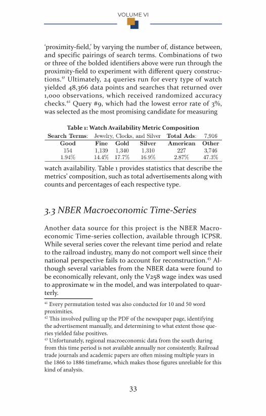
‘proximity-field,’ by varying the number of, distance between, and specific pairings of search terms. Combinations of two or three of the bolded identifiers above were run through the proximity-field to experiment with different query construc-tions.41 Ultimately, 24 queries run for every type of watch yielded 48,366 data points and searches that returned over 1,000 observations, which received randomized accuracy checks.42 Query #9, which had the lowest error rate of 3%, was selected as the most promising candidate for measuring
Table 1: Watch Availability Metric Composition
watch availability. Table 1 provides statistics that describe the metrics’ composition, such as total advertisements along with counts and percentages of each respective type.
3.3 NBER Macroeconomic Time-Series
Another data source for this project is the NBER Macro-economic Time-series collection, available through ICPSR. While several series cover the relevant time period and relate to the railroad industry, many do not comport well since their national perspective fails to account for reconstruction.43 Al-though several variables from the NBER data were found to be economically relevant, only the V258 wage index was used to approximate w in the model, and was interpolated to quar-terly.41 Every permutation tested was also conducted for 10 and 50 word proximities.42 This involved pulling up the PDF of the newspaper page, identifying the advertisement manually, and determining to what extent those que-ries yielded false positives.43 Unfortunately, regional macroeconomic data from the south during from this time period is not available annually nor consistently. Railroad trade journals and academic papers are often missing multiple years in the 1866 to 1886 timeframe, which makes those figures unreliable for this kind of analysis.
BERKELEY ECONOMIC REVIEW
34
4. Regression Analysis
Multivariate time-series regression was employed to measure the effect of increased watch availability on MTRR labor costs. An empirical analysis determined that the development of an innate sense of time-discipline was a statistically significant factor for workers bargaining for higher wages by initially us-ing this univariate regression equation:
∆ logLCt = βw∆ log Wt + εt,
where ∆logLCt is the first-difference of a log-transformed la-bor cost at time t, βW is the coefficient for the log-differenced watch availability metric ∆log Wt, and error term εt, to answer this research question.44 Prior to presenting the statistical re-sults, however, an aside to review the design of the time-disci-pline explanatory variable is necessary. This component over-comes the main obstacle to quantitatively discerning clock-time’s tangible effects. The following subsection presents multivariate regression results that provide robust support for the two hypotheses.
4.1 Watch Availability Metric
The metric’s construction draws on marketing literature to develop an accurate representation of local timepiece accessi-bility. While a long-form literature analysis in the Appendix,
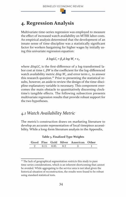
Table 3. Finalized Type-Weights
44 The lack of geographical segmentation restricts this study to pure time-series considerations, which is an inherent shortcoming that cannot be avoided. While aggregating to the service area is not ideal given the historical situation of reconstruction, the results were found to be robust using standard statistical tests.
VOLUME VI
35
the most crucial factors for the metric were determined to be:
• Visibility: derived from the page number in the paper the advertisement appeared on and scaled relative to the thickness of all newspapers in the county at the time
• Competition: the share of a paper’s advertisements in the county at the time45
• Frequency: the amount of times a particular paper was published per week
• Exposure: county level data for population in a given decade was combined with visibility to approximate the number of people reached46
• Relevance: the distance in miles from an advertisement’s county of publication to the nearest county with an MTRR station.47
In addition to marketing factors, assigning levels of accessibility to each type of timepiece is an essential part of the metric. Different watches sold for vastly different prices, and for good reason. Luxury timepieces represented status symbols and, when sold “at a high enough level [the] pricey prices may [have] actually stimulate demand.”48 Practical watches, however, told time and little else, meaning that buyers paid more for accuracy. Although many advertise-ments promoted low prices, few presented a range of price-points fully describing their stocks. This paper is primarily concerned with relative (rather than absolute) differences, 45 Grouping by advertiser was not possible and this ratio was used to capture a measure of market share in the local area.46 Data drawn per decade from population.us. Linear interpolation was used to fill in any gaps.47 Data drawn from distancefromto.net. Driving distance, instead of di-rect distance, was used to better approximate the overland travel required in the mid-nineteenth century.48 Landes, Revolution in Time, 355. Historians believe that these watches may have been Veblen goods.
BERKELEY ECONOMIC REVIEW
36
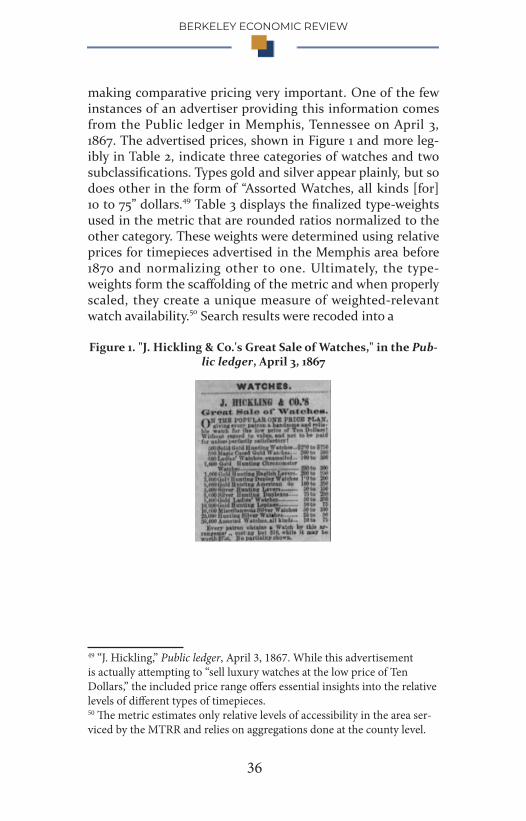
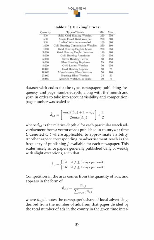
making comparative pricing very important. One of the few instances of an advertiser providing this information comes from the Public ledger in Memphis, Tennessee on April 3, 1867. The advertised prices, shown in Figure 1 and more leg-ibly in Table 2, indicate three categories of watches and two subclassifications. Types gold and silver appear plainly, but so does other in the form of “Assorted Watches, all kinds [for] 10 to 75” dollars.49 Table 3 displays the finalized type-weights used in the metric that are rounded ratios normalized to the other category. These weights were determined using relative prices for timepieces advertised in the Memphis area before 1870 and normalizing other to one. Ultimately, the type-weights form the scaffolding of the metric and when properly scaled, they create a unique measure of weighted-relevant watch availability.50 Search results were recoded into a
Figure 1. "J. Hickling & Co.'s Great Sale of Watches," in the Pub-lic ledger, April 3, 1867
49 “J. Hickling,” Public ledger, April 3, 1867. While this advertisement is actually attempting to “sell luxury watches at the low price of Ten Dollars,” the included price range offers essential insights into the relative levels of different types of timepieces.50 The metric estimates only relative levels of accessibility in the area ser-viced by the MTRR and relies on aggregations done at the county level.
VOLUME VI
37
Table 2. "J. Hickling" Prices
dataset with codes for the type, newspaper, publishing fre-quency, and page number/depth, along with the month and year. In order to take into account visibility and competition, page number was scaled as
where dˆc,t is the relative depth d for each particular watch ad-vertisement from a vector of ads published in county c at time t, denoted c, t where applicable, to approximate visibility. Another aspect corresponding to advertisement reach is the frequency of publishing f, available for each newspaper. This scales nicely since papers generally published daily or weekly with slight exceptions, such that
f^c,t = {0.4 if f ≤ 3 days per week
0.6 if f ≥ 4 days per week.
Competition in the area comes from the quantity of ads, and appears in the form of
n^c,t =
where ˆnc,t denotes the newspaper’s share of local advertising, derived from the number of ads from that paper divided by the total number of ads in the county in the given time inter-
BERKELEY ECONOMIC REVIEW
38
val. The six watch types, each referring to a vector of watch advertisements with the above attributes, factor into the met-ric according to their type-weight. The weight of a particular newspaper from a given county appear as
(4.1)
which denotes the sum of every advertisement-type vector’s elements scaled by the type- weight wc,t, relative depth, ad-vertisement share, and publishing frequency. All of the paper weights are aggregated to produce a raw county weight:
(4.2)
The next step involves scaling these weights by population and distance to reflect their exposure and relevance to the MTRR service area. Scaled county weights come from
(4.3)
where ρc is the population for each county in the decade en-compassing time t and δc is the distance to the closest county with an MTRR station. Counties with stations are assigned δc = 36 such that the construction (6/√δc) yields scaled distances between zero and one with higher values for those closer to MTRR activity. The raw metric of watch availability is the sum of all scaled county weights for each interval of time:
(4.4)
However, fewer raw watch advertisements did not necessarily mean less watch sales occurred, especially since the stores would not have disappeared completely in the absence of ads. Therefore, the metric used in the regressions is lagged, taking into account the past three years at each instance. This means the lagged measurement is:

VOLUME VI
39
(4.5)
where the vector {Lt} for t = [1866Q1, 1886Q4] is the weight-ed-relevant advertisement (WRA) metric of watch avail-ability. Figure 2 provides a graphical representation of this independent variable that depicts the trend upwards in watch availability during MTRR operations. The series has a mean of 13,428 and a standard deviation of 9,608 WRA units. An in-crease of one for the WRA metric is the equivalent of a front-page ad for a standard watch being run in the MTRR service area. There is also seasonality present, which is taken into consideration in the regression analysis.51
Regressing against the annual total of ads instead of the WRA metric does not account for different levels of ac-cessibility for distinct types of timepiece, or the importance of those ads for MTRR employees. Type-weights, along with other scalings methods encouraged by the secondary litera-ture, confer ‘weighting’ and ‘relevance’ stems from the likeli-hood of advertisement exposure to residents of DeSoto, Tate, Panola, Shelby, Grenada, Yalobusha, and Tallahatchie coun-ties.52 The regressions utilize the series in log-difference form to standard- ize its units as percent changes. Interpretations of the resulting coefficients assume that the WRA metric rep-resents a linear measure of watch availability proportional to the amount of money spent on obtaining these timepieces, which is justified by the literature review presented in the Appendix.
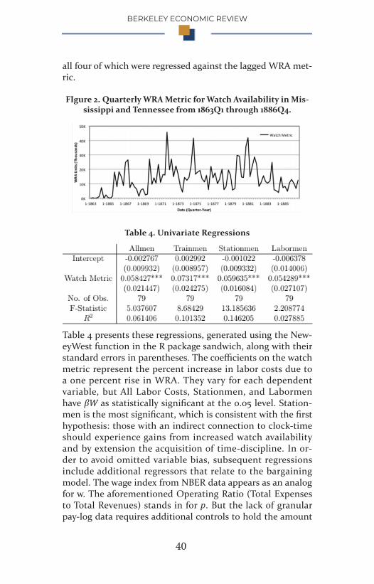
4.2 Regression Analysis
As mentioned previously, All Labor Costs for the MTRR can be disaggregated into Trainmen, Stationmen, and Labormen,
51 The fall-off in WRA can likely be attributed to the end of reconstruc-tion and the opening of new, more modern lines in adjacent counties.52 Robustness checks were also performed on weighted with and without relevance to determine that population shifts were not solely responsible for metric fluctuations.
BERKELEY ECONOMIC REVIEW
40
all four of which were regressed against the lagged WRA met-ric.
FIgure 2. Quarterly WRA Metric for Watch Availability in Mis-sissippi and Tennessee from 1863Q1 through 1886Q4.
Table 4. Univariate Regressions
Table 4 presents these regressions, generated using the New-eyWest function in the R package sandwich, along with their standard errors in parentheses. The coefficients on the watch metric represent the percent increase in labor costs due to a one percent rise in WRA. They vary for each dependent variable, but All Labor Costs, Stationmen, and Labormen have βW as statistically significant at the 0.05 level. Station-men is the most significant, which is consistent with the first hypothesis: those with an indirect connection to clock-time should experience gains from increased watch availability and by extension the acquisition of time-discipline. In or-der to avoid omitted variable bias, subsequent regressions include additional regressors that relate to the bargaining model. The wage index from NBER data appears as an analog for w. The aforementioned Operating Ratio (Total Expenses to Total Revenues) stands in for p. But the lack of granular pay-log data requires additional controls to hold the amount

VOLUME VI
41
of employed workers constant in the regressions.53 Total Rev-enue shifts reflect increased traffic in passenger and freight business that would have required employing more men and/or paying for more man-hours. Wood and Water expenses at stations, tracked by the MTRR, are also relatively proportion-al to the amount of activity along the line. Disease and mar-ket indicators capture pathogenic and financial complications that adversely affected operations.54 Additionally, quarterly indicators were included to account for seasonal fluctuations. These variables appear in the expanded regression equation:
∆ logLCt = βW ∆logWt + βX ∆ logXt + βIIt + μt
where βX is a vector of coefficients for the log-differenced re-gressors ∆logXt, βI is the coefficient vector for the indicators in It, and μt is another error term.
The results in the first four columns of Table 5 demonstrate the importance of additional regressors. The coefficient for the watch metric is now only statistically sig-nificant for Stationmen. Both All Labor Costs and Labormen are positive but insignificant, which further supports the first hypothesis. Therefore, those with either direct or non-existent connections to clock-time experienced no verifiable increase whereas those with an indirect connection have a positive, statistically significant relationship. The economic significance of time-discipline is apparent from the relative magnitude of the coefficient for the watch availability metric compared to the other potential determinants of Stationmen labor costs, provided one maintains the aforementioned lin-earity assumption.
Further indications of timepiece importance come from regressing certain granular worker- pay series against the same variables. Licht’s labor cost categories separate 53 While the MTRR archives include expense ledgers that have the occa-sional employee pay log, those figures were unusable for statistical testing due to data gaps and other inconsistencies.54 Both indicator coefficients are supposed to be negative, but in the instances where they are estimated as positive they are never statistically significant.
BERKELEY ECONOMIC REVIEW
42
employees by technical responsibilities, but the ‘Agents and Clerks’ in Stationmen and ‘Labor at Stations’ in Labormen worked alongside one another. Agents and Clerks had agency and incentives to work closely in accordance with clock-time whereas Station Laborers had neither. The watch metrics’ coefficients in last two columns of Table 5 support the second hypothesis by showing that nonexistent connections to clock-time negated the importance of time-discipline.
4.3 Summary of Results and Robustness Checks
In the tables above Stationmen and Agents and Clerks are the only labor costs that have positive, statistically significant relationships with the watch metric. They worked with an indirect connection to clock-time, which means these results validate the first hypothesis. Trainmen and Labormen, those with direct or nonexistent connections to clock-time, have insignificant regression coefficients, thereby supporting the second hypothesis. Moreover, Agents and Clerks and Station Laborers worked in the same places, such that the arrivals and departures of a locomotive would have alerted both class-es of employees to the time. Yet only the former exhibits a positive, statistically significant relationship to the increased availability of watches. Laborers, even in the presence of a clock, worked irrespective of the hour and thusly experienced no gains from greater timepiece accessibility. This comparison confirms both hypotheses and demonstrates that those with sufficient agency, awareness, and incentives to utilize tempo-ral information benefited from obtaining watches. The mi-croeconomic implications for those with positive, statistically significant relationship to time-discipline were increased bar-gaining power when negotiating wages.
Employees in possession of watches could theoreti-cally resist unwitting exploitation and command higher sala-ries. These findings validate the central premise of Thompson (1967) for specific kinds of railroad workers and have im-
VOLUME VI
43
plications for other nineteenth century American laborers. Furthermore, the regression coefficients comport favorably with the Pissarides (2000) model analysis. While MTRR tex-tual sources omit wage negotiations, these results indicate that technological change did enhance the bargaining power of workers. The WRA metric also received robustness checks that demonstrate the importance of weighting it by watch type and the viability of its design. Alternative type-weights were substituted into all regression equations. Uniform and counteracting weights produced result that could not be interpreted, thereby indicating the importance of correctly type-weighting the metric.Weights drawn directly from the price ratios (unrounded) produced coefficients consistent with the results for the labor cost categories. In every case Labor at Stations always had p-values that were larger than Agents and Clerks’ and/or were not statistically significant, which maintains sufficient support for the above results.
Another robustness check, mentioned in the model section, is the inclusion of another technological change vari-able. The MTRR accounted for its telegraph expenses, which allows this paper to perform a third type of regression:
∆ log LCt = βT ∆logTt + βW ∆logWt + βX ∆logXt + βIIt + ξt
where βT is the coefficient for log-differenced telegraph ex-penses ∆log Tt and ξt is another error term. Table 6 displays the regression results for all of the aforementioned labor costs and the βW coefficients for Stationmen and Agents and Clerks are both still statistically significant. βT is significant for Stationmen, which does imply that an increase in general technology could capture the some effects of time-discipline, but the persistence of the WRA metric significant confirms the benefit from purchasing watches. Additionally, the lack of significance for Labormen shows work devoid of dependence on technology was not affected by general advancements. De-termining that generic railroad technological improvements, as represented by telegraph signaling, cannot receive full credit for gains attributable to time-discipline thusly provides additional quantitative support for Thompson (1967).
BERKELEY ECONOMIC REVIEW
44
5. Conclusion
The continued importance of clock-time and minimum wage work means that empirically validating Thompson’s thesis has implications for contemporary labor studies. The con-clusions of this paper indicate that those without agency, the unskilled workers of today, are susceptible to exploitation due to technology asymmetry. A recently published NBER work-ing paper from Acemoglu and Restrepo (2017) argues that automation has quantifiably adverse consequences for certain types of workers. While technological advances towards a shared economy might enable everyday people to leverage time-discipline, those still employed in hourly work need to retain their agency in a race against machines.
The empirical data approach should be applied to studies of modern innovations that affect work, most of which rely on a foundation of time-discipline conferred by ubiquitous clocks. Moreover, the availability of historical data and statistical tools creates ample opportunity for further analysis of numerous important inventions. Clock-time ulti-mately ushered in certain aspects of the modern world, but more recent developments also require attention from econo-metricians to discern the implications of new technology adoption.
VOLUME VI
45
6. Appendix
6.1 MTRR Labor Costs
Railroads across America accounted for payments to their employees in different ways, and below are the MTRR’s labor costs with brief descriptions of their responsibilities:
• Agents and Clerks: Railroads employed multiple kinds of agents, including Station Agents in charge of the railroad station, Ticket Agents selling tickets and answered questions, and Express Agents ship ping packages. The MTRR did not disambiguate the types of agents in their expense reports or routinely in the ledgers. Clerks often engaged with passengers at the direction of agents.
• Baggage Masters: These employees handled passenger items, tagging and unloading them at the proper stations.
• Brakemen: Prior to the introduction of airbrakes in the late nineteenth century railroads employed men to apply the brakes by turning brake wheels on the top of each car when the engineer signaled to stop the train.
• Conductors: Responsible for everybody aboard the train, they ordered trains to leave stations, when to apply the brakes upon arrival, and engaged with passengers.
• Engineers and Firemen: The MTRR accountants combined these two related, yet very distinct, roles. Engineers were responsible operating the locomotive and if it needed repairs they fixed it. Fireman fed the firebox with fuel while the engine was in use, putting them under the direct supervision of engineers.
BERKELEY ECONOMIC REVIEW
46
• Labor at Stations: Instead of grouping all labor under one expense, the MTRR dis- aggregated its costs into three categories. Station labor often took the form of minor repairs and unloading freight.
• Machinists and Laborers: These workers performed skilled and semi-skilled labor repairing engines in the railroad shops.
• Track Labor: Workers would replace cross ties in the track and lay new rails if necessary, although this depended on a variety of factors including wear and tear, weather damage, and the price of materials.
• Yardmasters and Switchmen: The MTRR also combined these two classes of related workers, in this case the those that worked in the yard. Yardmasters were in charge of switching and yard operations while Switchman worked in the railroad yards aligning the track switches and hooking cars together.
• Watchmen: Each division of the MTRR had watchmen, whom Licht includes with other station employees.55 Consolidating these line items created a composite series for all watchmen.56
6.2 Watch Advertisement Qualitative Analy-sis
O’Malley (1990) and Landes (1983) extensively reviewed how certain advertising themes made watches more than just sta-tus symbols; they stressed their importance for developing an innate sense of time-discipline inaccessible to those without a timepiece. But while the former vastly extended the latter’s 55 Litch, Working for the Railroad, 14.56 Annual reports do not include data for Yardmasters and Switchmen or Watchmen expense until 1871, as such they only appear in aggregated measures of labor cost.
VOLUME VI
47
observations, both historians focused almost exclusively on national ad campaigns and avoided consideration of smaller retailers selling watches along with other items. Their analysis supports the use of watch advertisements as a proxy for time- discipline acquisition, but limiting data collection to the pro-motions of large corporations inherently narrows the scope of this project and thusly requires additional assessments of adverts in the MTRR service area.
Local timepiece retailers in the mid-nineteenth cen-tury utilized a few select adjectives to entice particular types of interested buyers. Generally sold by jewelers, gold and silver watches were luxury items that could “announce one’s exclusivity and success” to fellow socialites.57 Advertisements for these particular timepieces often appeared as part of broader appeals to wealthier patrons; W.H. Calhoun & Com-pany, “importers, manufacturers, and dealers [of] fine watch-es, diamond and fashionable jewelry, [also advertised] SOLID SILVER [items such as] silver-plated ware, clocks and fancy goods” to readers of the Nashville Union and American.58 Similarly, the Memphis daily appeal displayed an advert for the “fine gold watches and chains [sold by] F.D. Barnum & Co. [as] new & rich jewelry.”59 Both described the luxury watches as “fine,” a seemingly benign adjective that consistently ap-peared in advertisements targeting customers buying other expensive items. These advertisements also referenced other wares sold by jewelers: silver(ware), clocks, diamonds, chains, and, of course, jewelry. L. Gauchat in Clarksville, Tenn. ad-vertised itself as a “dealer in fine watches, jewelry, clocks and silverware” in another appeal to upper class customers.60 Merchants focused on selling luxury watches put them at the top of their lists but also mentioned other luxury goods. Al-though many vendors described their wares as ‘fine,’ the term generally referred to gold and silver varieties that appealed to richer patrons when applied to watches.
57 Landes, Revolution in Time, 355.58 “F.L. Davies & Bro,” The Nashville Union and American, April 2, 1874. All newspaper names are written as they appear in CA.59 “New Advertisements,” The Memphis daily-appeal, August 24, 187060 “L. Gauchat,” Clarksville Weekly Chronicle, June 7, 1879.

BERKELEY ECONOMIC REVIEW
48
Retailers targeting less lavish clientele employed other adjectives that indicated lower prices. An advertise-ment in The Daily clarion called attention to “a large stock of goods [for] retail at wholesale prices [including] fancy goods, watches, [and] clocks.”61 This advert assigned no adjective to watches, listed other items with only the descriptor “fancy,” and emphasized their inexpensiveness using on ‘wholesale prices’ to attract patrons. Moreover, when an F.D. Barnum ad-vertisement in the Memphis daily appeal appeared alongside a competitor, it emphasized “$5 [and] $8 good WATCHES at old prices [as distinct from the] Massive Oride Gold Dou-ble Hunting Magic Spring Case” watch noted adjacently.62 ‘Good’ watches therefore, did not refer to the same expensive timepieces in as those identified as ‘fine.’ The two conven-tions even appeared alongside one another when “W.H. Kirk, watchmaker, [advertised] watches, clocks, jewelry and sport-ing goods[, specifically] orders for fine GOOD WATCHES.” 63This double qualification and mismatched capitalization implies that the two descriptors referred to different market segments. Surveying numerous advertisements reveals that ‘good’ watches were advertised with lower price points than ‘fine’ watches to target budget-conscious buyers. Other de-scriptor for cheaper timepieces include ‘Ameri- can,’ often used alongside the term ‘Swiss Watches’ to indicate lower prices.64
Analyzing the adjectives utilized by advertisers il-luminates specific categories of time- pieces for estimating levels of watch availability and the ‘phrase-field’ allowed for the pinpointing of word groups associated with certain variants of watches. The six types form the scaffolding of the metric of watch availability. Searching a database for adverts distinguished by these categories required particular query construction to avoid noise. Therefore combinations of the words ‘goods’, ‘jewelry’, ‘clocks’, and ‘silver’ were included in each query.61 “J. S. Hendrickson,” The Daily clarion, December 9, 1866.62 “New Advertisements,” The Memphis daily-appeal, August 24, 1870.63 “W.H. Kirk,” The Maryville times, January 8, 1885.64 “Notice to the Public,” The Pascagoula democrat-star, February 27, 1880.
VOLUME VI
49
6.3 Local Advertising Literature Analysis
Nowak, Cameron, and Krugman (1993) found that “local marketers [devote] more resources to response-oriented me-dia and [place] less emphasis on image-oriented mass media advertising.”65 Their analysis applies directly to this study since 77% of local advertisers surveyed in 1993 still used dai-ly newspapers as their primary promotional medium, with 69% of advertising budgets spent on some form of periodical. After categorizing businesses the relevance increases: 74.4% of “General merchandise” shops used the “Daily paper,” more than any other kind of media. The investigators also asked local advertisers to rank on a one-to-five scale the most im-portant “media decision-making factors.” At the top were the “number of people who will see [the] ad (4.8), ability to target/reach specific audiences (4.6), number of times [the] ad [would] appear (4.2), ability to generate immediate store traffic (4.2), [and the] ability to reach the entire market (3.8).”66 Five of the top six factors pertain directly to mid-nineteenth century watch advertising and thusly indicate the advertising priorities that inform the metric construction.
In a related study, Reibstien and Traver (1982) sought to determine which factors had a quantifiable impact on cou-pon redemption rates. Their first table has some overlap in the areas of distribution methods and audience reached, but the paper also stresses the importance of competitive factors such as market share, competitor activity, and branding.67 These concerns ranked only at 2.7 for General merchandis-ers in the later survey,68 but more recent scholarship from Azarnoush and Riasi (2016) has shown “competitiveness is positively related to brand advertising success and effective-
65 Glen J. Nowak, Glen T. Cameron, and Dean M. Krugman, “How Local Advertisers Choose and Use Advertising Media.” Journal of Advertising Research, (November/December, 1993), 39.66 Ibid., 43-5.67 David J. Reibstien and Phillis A. Traver, “Factors Affecting Coupon Redemption Rates,” Journal of Marketing (46, No. 4, 1982), 10468 Nowak, Cameron, and Krugman, “How Local Advertisers Choose and Use Advertising Media,” 45.
BERKELEY ECONOMIC REVIEW
50
ness.”69 Therefore, at each time interval the metric also takes into account the total amount of advertisements in a specific area to account for the level of competition.
69 Azarnoush Ansari and Arsh Riasi, “An Investigation of Factors Affect-ing Brand Advertising Success and Effectiveness,” International Business Record (9, No. 4, 2016), 26.

VOLUME VI
51
7. References
Acemoglu, D., P. Antr`as, and E. Helpman (2007). Contracts
and technology adoption. The American Economic
Review 97(3), 916–943.
Acemoglu, D. and P. Restrepo (2017, March). Robots and Jobs:
Evidence from US Labor Markets. Working Paper
23285, National Bureau of Economic Research.
Azarnoush, A. and A. Riasi (2016). An Investigation of Factors
Affecting Brand Advertising Success and
Effectiveness. International Business Record 9(4),
20–30.
Bhaskar, V. and T. To (1999). Minimum Wages for Ronald
Mcdonald Monopsonies: A Theory of Monopsonistic
Competition. The Economic Journal 109(455), 190–
203.
Bils, M., Y. Chang, and S.-B. Kim (2011). Worker
Heterogeneity and Endogenous Separations in a
Matching Model of Unemployment Fluctuations.
American Economic Journal: Macroeconomics 3(1),
128–154.
Boerner, L. and S. Battista (2016, February). Time for Growth.
Bryan, M. L. (2006). Free to Choose? Differences in the Hours
Determination of Constrained and Unconstrained
Workers. Oxford Economic Papers.
Calmès, C. et al. (2005). Self-Enforcing Labour Contracts
and the Dynamics Puzzle. Bank of Canada.
Crafts, N. (2002). The Solow Productivity Paradox in
Historical Perspective.
David, P. A. (1990). The Dynamo and the Computer: An
BERKELEY ECONOMIC REVIEW
52
Historical Perspective on the Modern Productivity
Paradox. The American Economic Review 80(2),
355–361.
Dittmar, J. (2011). The Welfare Impact of a New Good: The P
rinted Book. Department of Economics, American
University.
Dohrn-van Rossum, G. (1996). History of the Hour: Clocks
and Modern Temporal Orders. Chicago: University
of Chicago Press.
Ebell, M. and C. Haefke (2004). The Missing Link: Product
Market Regulation, Collective Bargaining and the
European Unemployment Puzzle. In Society for
Economic Dynamics, Meeting Papers, Volume 579.
Ferguson, W. D. (1994). Union Bargaining Power in an
Efficiency Wage Environment. Eastern Economic
Journal 20(4), 387–401.
Gertler, M., L. Sala, and A. Trigari (2008). An Estimated
Monetary DSGE Model with Unemployment and
Staggered Nominal Wage Bargaining. Journal of
Money, Credit and Banking 40(8), 1713–1764.
Gertler, M. and A. Trigari (2009). Unemployment
Fluctuations with Staggered Nash Wage Bargaining.
Journal of Political Economy 117(1), 38–86.
Grossman, G. M. and E. Helpman (1991). Trade, Knowledge
Spillovers, and Growth. European Economic Review
35(2-3), 517–526.
Kahn, S. and K. Lang (1991). The Effect of Hours Constraints
on Labor Supply Estimates. The Review of
Economics and Statistics, 605–611.
Kahn, S. and K. Lang (1996). Hours Constraints and the
VOLUME VI
53
Wage/Hours Locus. The Canadian Journal of
Economics/Revue Canadienne d’Economique 29,
S71–S75.
Landes, D. (1983). Revolution In Time: Clocks and the
Making of the Modern World. Cambridge: Harvard
University Press.
Licht, W. (1983). Working for the Railroads: The
Organization of Work in the Nineteenth Century.
Princeton: Princeton University Press.
Marrs, A. W. (2009). Railroads in the Old South: pursuing
progress in a slave society. Baltimore: The Johns
Hopkins University Press.
Mumford, L. (1934). Technics and Civilization. New York:
Harcourt, Brace and World.
Naylor, R. A. (2002, March). Labour Supply, Efficient Bargains
and Countervailing Power.
Nowak, G. J., G. T. Cameron, and D. M. Krugman (1993). How
Local Advertisers Choose and Use Advertising
Media. Journal of Advertising Research (November/
December), 39– 49.
O’Malley, M. (1990). Keeping Watch: A History of American
Time. New York: Penguin Group.
Pissarides, C. (2000, March). Equilibrium Unemployment
Theory. Boston: MIT Press.
Pissarides, C. A. (1985). Short-run Equilibrium Dynamics of
Unemployment, Vacancies, and Real Wages. The
American Economic Review 75(4), 676–690.
Reibstien, D. J. and P. A. Traver (1982). Factors Affecting
Coupon Redemption Rates. Journal of Marketing
46(4), 102–113.
BERKELEY ECONOMIC REVIEW
54
Rotemberg, J. J. (2000, October). Wages and Labor demand
in an Individualistic Bargaining Model with
Unemployment.
Shapiro, C. and J. E. Stiglitz (1984, June). Equilibrium
Unemployment as a Worker Discipline Device. The
American Economic Review 74(3), 433–444.
Stewart, M. B. and J. K. Swaffield (1997). Constraints on the
Desired Hours of Work of British Men.
The Economic Journal 107(441), 520–535.
Stole, L. A. and J. Zwiebel (1996a). Intra-firm Bargaining
under Non-binding Contracts. The Review of
Economic Studies 63(3), 375–410.
Stole, L. A. and J. Zwiebel (1996b). Organizational Design and
Technology Choice under Intrafirm Bargaining. The
American Economic Review, 195–222.
Strand, J. (2003). Wage Bargaining Versus Efficiency Wages: a
Synthesis. Bulletin of Economic Research 55(1), 1–20.
Thompson, E. (1967, December). Time, Work-discipline and
Industrial Capitalism. The Past and Present Society
(38), 56–97.
Trigari, A. (2006). The Role of Search Frictions and
Bargaining for Inflation Dynamics.

VOLUME VI
55
[THIS PAGE INTENTIONALLY LEFT BLANK]

BERKELEY ECONOMIC REVIEW
56
The Sino-African Relationship: An Empirical Study of the Effect of Chinese Foreign
Direct Investment on Illicit Financial Flows in Africa
Fatima Ezzahra DaifYale-NUS College
AbstractForeign Direct Investment (FDI) in the African continent, particularly Chinese-led investment, has been criticized in recent years for lacking adequate regulatory frameworks and enabling high-level corruption. This is an alarming criticism given that Beijing is today a major provider of FDI capital in Africa, and at the same time, African countries are estimated to collectively lose $30-$60 billion USD to illicit financial flows (IFFs) every year. However, there is little systematic evidence to support these criticisms and determine whether anecdotal evidence reflects the true effect of Beijing’s investments. This study aims to address that gap by providing causal estimates of the effect of Chinese FDI on IFFs in recipient African countries. We use an instrumental variable strategy that exploits variation in FDI volumes due to two factors -- exogenous variation in Chinese steel production and the cross-sectional variation in a country’s likelihood of dealing with Chinese firms. We find that a $1 increase in Chinese FDI increases the volume of illicit financial flows by $3.72, a result that is statistically significant. Conversely, we find no evidence of FDI triggering the first onset of illicit financial activity; instead, FDI appears to exacerbate existing volumes of IFFs. Our findings also suggest that the effects of FDI are most pronounced in the year in which it is received.

VOLUME VI
57
TABLE OF CONTENTS
1. Introduction 592. Literature Review 633. Institutional Background 66 3.1. Chinese FDI and IFFs 66 3.2. Determinants of Chinese FDI 674. Empirical Strategy 695. Data and Descriptive Statistics 726. Estimation Results and Discussion 76 6.1. OLS Estimates and Reduced-Form Estimates 76 6.2. First-Stage Estimates 77 6.3. 2SLS Estimates 78 6.4. Controlling for Lagged Illicit Financial Flows 79 6.5. Falsification Tests 80 6.6. Additional Robustness Checks 817. Mechanisms 848. Heterogeneous Effects of Chinese FDI 859. Limitations 8810. Conclusion 8911. References 91
List of Figures
Figure 1. Chinese FDI And Previous Year's Chinese Steel Production 73
Figure 2. Average IFFs And Previous Year’s Steel Production, Frequent Recipients 74
Figure 3. Average IFFs And Previous Year’s Steel Production, Infrequent Recipients 75
BERKELEY ECONOMIC REVIEW
58
List of Tables
Table 1. Descriptive Statistics 73
Table 2. The Effect of Chinese FDI On IFFs: OLS And Reduced-Form Estimates 76
Table 3. First Stage Estimates with P t−1 × Di As the Instrument for FDI 77
Table 4. 2SLS Regression with Pt−1 × Di As the Instrumental Variable 78
Table 5. The Effect of FDI on IFFs: Controlling for Lagged Dependent Variable 80
Table 6. Falsification Tests: Effect of The Instrument on Past FDI 81
Table 7. The Effect of FDI On IFFs: Robustness to Alternative Specifications 83
Table 8. The Effect of FDI On the Onset and Scale of IFFs 84
Table 9. Heterogeneous Effects of FDI on IFFs 87
Abbreviations and Acronyms
FDI Foreign Direct Investment
IFFs Illicit Financial Flows
GFI Global Financial Integrity
UNCTAD United Nations Conference on Trade and Development
OLS Ordinary Least Squares
2SLS Two-Stage least squares
VOLUME VI
59
1. Introduction
Foreign direct investment (FDI)1 is an important catalyst for economic growth in developing nations. It enables capital-poor nations to build physical capital, diversify their economies, create jobs, and transfer both technical and managerial skills to local labor. While the lion’s share of global FDI has been led by the European Union (EU) and the United States, China has emerged over the last three decades as an important investment partner for the Global South, particularly on the African continent.2 The China-Africa Trade and Economic Cooperation reported that Beijing’s FDI outflows to Africa grew by a yearly average of 20.5% in the past decade. In 2016, China’s FDI to Africa stood at US $36.1 billion, making the country the “largest contributor of FDI capital and jobs” on the African continent that year.3
However, as China’s economic reach has expanded, so has the criticism of the efficacy of its FDI, especially in regions where governance institutions are weak. Reports of African presidents receiving monetary inducements to green light Chinese projects have made headlines in recent years.4 Such stories are not uncommon: In political science literature, Chinese FDI has been associated with no-strings-attached policies and has often been criticized for lacking adequate regulatory frameworks (such as anti-bribery laws that govern business done abroad).5 Moreover, Chinese-led projects are reportedly made at the highest political levels, involve ambiguous bidding processes, and most include extensive leeway for local leaders to direct funding and staffing on the ground.6 As such, economists, journalists and development institutions have noted that Chinese FDI projects are uniquely positioned to offer both a high incentive
1 Defined as investment by privately-owned companies based in one country in business interests in a foreign country.2 Buckley, 20043 Earnst and Young, 20174 Marsh, 20185 Buckley, 20046 Jayaram, Kassiri and Sun, 2017
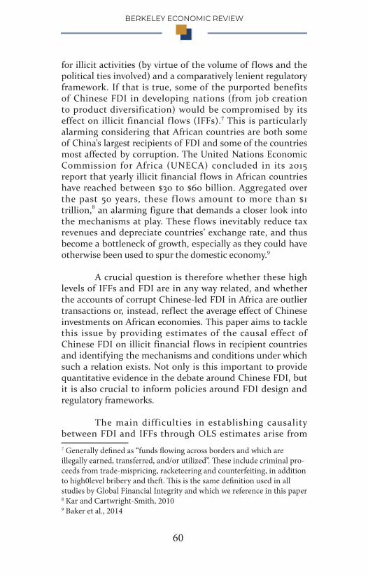
BERKELEY ECONOMIC REVIEW
60
for illicit activities (by virtue of the volume of flows and the political ties involved) and a comparatively lenient regulatory framework. If that is true, some of the purported benefits of Chinese FDI in developing nations (from job creation to product diversification) would be compromised by its effect on illicit financial f lows (IFFs).7 This is particularly alarming considering that African countries are both some of China’s largest recipients of FDI and some of the countries most affected by corruption. The United Nations Economic Commission for Africa (UNECA) concluded in its 2015 report that yearly illicit financial flows in African countries have reached between $30 to $60 billion. Aggregated over the past 50 years, these f lows amount to more than $1 trillion,8 an alarming figure that demands a closer look into the mechanisms at play. These f lows inevitably reduce tax revenues and depreciate countries’ exchange rate, and thus become a bottleneck of growth, especially as they could have otherwise been used to spur the domestic economy.9
A crucial question is therefore whether these high levels of IFFs and FDI are in any way related, and whether the accounts of corrupt Chinese-led FDI in Africa are outlier transactions or, instead, reflect the average effect of Chinese investments on African economies. This paper aims to tackle this issue by providing estimates of the causal effect of Chinese FDI on illicit financial f lows in recipient countries and identifying the mechanisms and conditions under which such a relation exists. Not only is this important to provide quantitative evidence in the debate around Chinese FDI, but it is also crucial to inform policies around FDI design and regulatory frameworks.
The main difficulties in establishing causality between FDI and IFFs through OLS estimates arise from 7 Generally defined as “funds flowing across borders and which are illegally earned, transferred, and/or utilized”. These include criminal pro-ceeds from trade-mispricing, racketeering and counterfeiting, in addition to high0level bribery and theft. This is the same definition used in all studies by Global Financial Integrity and which we reference in this paper8 Kar and Cartwright-Smith, 20109 Baker et al., 2014
VOLUME VI
61
reverse causality and joint determination—i.e. that more corrupt nations inherently attract more Chinese FDI, or that exogenous factors drive both variables in the same direction. For example, we would observe an upward bias in OLS estimates if the presence of IFFs is associated with a higher demand for Chinese FDI, potentially because corrupt leaders seek out lenient providers of capital. Similarly, exogenous factors can cause an upward bias in OLS estimates—one such an example is a surge in global demand for a country’s natural resources, which would increase both illicit activity (by increasing the gains from IFFs) and FDI (by attracting investments to resource-rich markets). Chinese FDI might also be directed towards countries with lower initial IFFs, in which case OLS estimates would be biased downwards.
This paper develops a novel instrumental variable approach to estimate the causal effect of Chinese FDI on illicit financial f lows on the African continent. Our instrument is the interaction term of Chinese steel production and the country’s likelihood of receiving FDI from China (measured as the proportion of years in the sample period in which the country gets a positive amount of FDI). The motivation behind this is that variation in Chinese steel production is primarily driven by domestic demand for steel (and so it is exogenous) and is shown to strongly predict future Chinese FDI (which, in Africa, is largely made up of infrastructure and steel-heavy projects). The country-variation in the likelihood of being a recipient of FDI differentiates between frequent and infrequent business partners of China, and thus strengthens the first stage assumption. This strategy is inspired by Nunn and Qian (2014) who estimated the effect of US food aid on conflicts and instrumented food aid with the interaction of food production and the likelihood of receiving US aid. We use a panel data set of 50 African countries from 2004 to 2015. We use data by Global Financial Integrity which estimates IFFs on the African continent using macroeconomic data, including: 1) mis-invoicing and discrepancies in countries’ trade statistics vis-à-vis their trade partners and 2) omissions in the balance of payments records.10
10 The explanation of the methodology is provided by Global Financial Integrity
BERKELEY ECONOMIC REVIEW
62
The main outcome of interest is the volume of illicit financial f lows in a country in a year. The OLS estimates of the effect of FDI on IFFs are positive and statistically significant at the 1% level and show that a $1 increase in FDI is associated with an additional $0.8 in IFFs. The 2SLS estimates, on the other hand, indicate that a $1 increase in Chinese FDI leads to a $3.72 increase in IFFs. To test the robustness of our strategy, we provide specifications where we control for lagged IFFs, test for contemporaneous effects, and examine heterogeneity among recipient countries. Overall, our results suggest that the effects of FDI are most felt in the years in which they are received, but that they do not vary significantly with countries’ income, democratic institutions and natural resource dependency. This said, our tests of the mechanisms underlying this relationship show that Chinese FDI has no effect on the first onset of IFFs, meaning that these deals likely do not trigger illicit activity in recipient countries but rather exacerbate it.
The rest of the paper is structured as follows: Section 2 provides an overview of the existing literature on this topic; Section 3 provides some background on the relationship between FDI and IFFs, and the determinants of Chinese FDI; Sections 4 and 5 describe the data and identification strategy; Section 6 presents our main results; Sections 7 and 8 examine the mechanisms and heterogeneous effects underlying our findings; Section 9 outlines the limitations of this study; and Section 10 concludes.

VOLUME VI
63
2. Literature ReviewOur study adds to a growing body of literature in both development economics and political science, particularly on the trade-offs involved in FDI, between promoting economic activity and potentially harming domestic markets. Choe (2003) for instance uses a VAR model and macroeconomic data from 1971 to 1995 to test the causal effect of FDI on economic outcomes. He finds that economic growth increases the inflow of foreign investments, but that the opposite is not true, as an increase in FDI inflows does not correspond to significant economic advantages for recipient countries. Similarly, Vu, Gangnes and Noy (2008) examine the causal effect of sector-specific FDI on growth in emerging markets. They show that FDI inflows positively impact labor-intensive sectors such as manufacturing but have little effect on other sectors. This then suggests mixed evidence on the efficacy of FDI and reiterates the need for systematic and quantitative estimates of their effect on various economic variables—including illicit financial activity.
Our focus on Chinese FDI also adds to an expanding literature on China’s role in the global economy. For instance, our findings are in line with evidence provided by Isaksson and Kotsadam (2016) who note that “more widespread local corruption around active, as compared to not-yet-opened, Chinese project sites (in African countries)”. To argue this, the authors use a difference-in-differences approach and match georeferenced project-level data (Chinese projects in Africa from 2000-2012) with respondents from four waves of surveys (on direct experiences with petty corruption). This then suggests a potential ‘China-effect’ on developing countries and supports our emphasis on China-led projects as potential channels for IFFs. The authors also provide anecdotal evidence of illicit financial activity around Chinese project sites, and our study corroborates those accounts and quantifies their average effect through causal empirical evidence. In the same vein, Morck, Yeung and Zhao (2008) use case studies to show that Chinese FDI is biased towards tax havens, and is often led by state-controlled enterprises,

BERKELEY ECONOMIC REVIEW
64
suggesting that firms might be targeting countries with whom Beijing has political ties. This then sets the stage for our discussion on China’s effect on illicit activity in African countries, which are some of Beijing’s largest FDI recipients.
However, there is growing evidence that counters this narrative and shows that, on balance, China’s effect on developing markets is positive. Jayaram and Sun (2017) of Mckinsey examine privately-owned firms operating in African countries and their overall impact on economic variables. They find that despite a number of labor and environmental violations, the overall effect of Chinese projects is positive. In fact, they note that 50% of the firms have introduced novel products or services to the local economy, and about 40% have lowered the price of existing products through economies of scale. This then suggests a mixed outlook on China’s African presence and echoes the need for more quantitative evidence on Beijing’s economic impact on African countries, rather than lone-standing accounts of success or failure.
Moreover, the topic of illicit financial activity has been at the core of development debates in recent years, especially after the United Nations adopted the Sustainable Development Goals 2015, one of which is reducing IFFs. As such, our findings add to a growing body of literature on the determinants of illicit financial f lows. Ndikumana and Boyce (2010) use omissions from countries’ balance of payment accounts to estimate capital f light in sub-Saharan Africa. In the same vein, the 2015 African Union Panel on Illicit Financial Flows provides quantitative estimates of illicit activity in Africa and argues that such f lows are strongly associated with weak political institutions and poor rule of law, and thus must be tackled systematically. This reiterates the significance of our study and helps us bound our estimates of Chinese-caused IFFs within the larger literature. Building on these findings, scholars have also compared inf lows to developing countries and IFFs arising from tax evasion and trade misinvoicing. Research by UNECA and the African Union has found that Africa alone loses between $30
VOLUME VI
65
to $60 billion in illicit financial flows every year, compared to $19bn received in aid, meaning as much as 3 times the aid amount that flows in is lost to IFFs. The authors argue that IFFs lead to a situation where development program work “in reverse” and are draining recipient countries instead of propelling them to economic prosperity. While this does not establish causality, it is starting point in understanding the magnitude of problem and the underlying mechanisms that our study ought to consider.
Overall, the literature surveyed provides mixed evidence on the link between FDI and economic growth, and points to a gap in knowledge in the mechanisms behind said relationship. More importantly, while these studies show the scale of illicit financial flows and point to the high level of corruption in Chinese project sites, they offer little empirical evidence on China’s causal and systematic effect on illicit financial activity in Africa, and the field still lacks quantitative estimates of the scale of such an effect. It is this gap that our study aims to fill. In addition, little is known on the political and socio-economic conditions that make this effect more prominent in one country over another. Our study thus attempts to differentiate between the effect of FDI on countries with different levels of GDP, natural resource endowment and political institutions.
BERKELEY ECONOMIC REVIEW
66
3. Institutional Background
3.1 Chinese FDI and IFFsAnecdotal evidence points to large-scale illicit financial flows where Chinese conglomerates are involved. In 2018 for instance, a Hong Kong financial mogul offered the president of Chad a $2 million bribe to secure oil rights for a Chinese corporation. In 2014, the former Secretary for Home Affairs of Hong Kong was accused of extending a $500,000 bribe to the foreign minister of Uganda for preferential treatment in a business bidding.11 Such deals indicate a trend of illicit activity tied to Chinese businesses. Indeed, critics of Beijing point to a mechanism by which Chinese FDI is linked to capital loss at a higher rate than their American or European counterparts—FDI seems to be a way for Chinese firms to build alliances with political leaders in emerging markets and secure concessions and commercial advantages (such as access to natural resources), with the “comparative advantage of no domestic legislation to answer to”.12 Moreover, FDI is thought to increase the share of resources that are “up for grabs” on the ground and, by extension, increase the returns to illicit activity.13 Chinese FDI projects are therefore uniquely positioned to offer both a high incentive for illicit activity (by virtue of the volume of flows involved) and few checks and balances (by recipient countries or Beijing itself).
These mechanisms are further supported by the divergence between regulations adopted by China compared to their American or European counterparts. While Beijing technically adopted the United Nations Convention Against Corruption in 2011, including its foreign bribery clauses, the government has not enforced it in practice.14 In fact, Beijing does not require Chinese firms and their partners to agree to anti-corruption measures before signing a deal, nor does it monitor the use of the proceeds from Chinese-led 11 Marsh, 201812 Tull 2006; Kaplinsky et al., 200713 Ibid14 Lang, 2017
VOLUME VI
67
projects. The result, as Kennan (2009) notes, is that “China's approach not only provides potentially corrupt leaders more opportunities to enrich themselves … it also does not hold accountable those leaders who do so”. In contrast, American firms aiming to do business abroad are legally bound by the Foreign Corrupt Practices Act (FCPA)15, British companies are required to abide by the UK Bribery Act,16 and OECD countries have agreed to an Anti-Bribery Convention,17 all of which stipulate that companies and individuals can be prosecuted for illicit financial activities committed abroad, and thus represent a major deterrent against illicit activity in international business dealings. These regulations have also been heavily enforced—in 2017, for instance, engineering company Technip paid $338 million to the SEC over charges of bribing Nigerian government officials to win construction contracts.18
These discrepancies in regulatory standard and enforcement track records not only mean that China has a relative advantage in the number of investment opportunities that it can pursue, but also that Chinese firms allow more scope for IFFs in their foreign engagements. Our focus on China in this study is therefore driven by both its position as an important global economic player and the distinct regulatory framework that governs its cross-border financial transactions.
3.2 Determinants of Chinese FDIOne such a commodity is steel. China is the world’s
15 This act was introduced by the Securities Exchange Act of 1934. It sets accounting transparency standards and limits payments to foreign political entities.16 The Act was introduced in 2010 and among other things, includes criminal and civil liability for foreign bribery.17 The Convention was signed in 2009 and criminalized bribery in foreign business transactions carried out by firms based in the OECD countries18 These charges are outlined in the SEC’s website under ‘Spotlight on Foreign Corrupt Practices Act’

BERKELEY ECONOMIC REVIEW
68
largest steel manufacturer,19 and studies have shown that f luctuations in domestic demand for steel determine the level of infrastructure projects that Chinese firms engage in internationally. For instance, Chinese steel production has increased 12-fold in the past 25 years, owing to Beijing’s massive domestic demand for steel during the boom years.20 However, domestic demand for steel has been affected by the current slowdown and is expected to decrease as the government moves from an investment-led/construction-driven strategy to a consumption-led economy (De Carvalho, 2017).21 Beijing’s oversupply of steel has then resulted in Chinese producers channeling their extra output towards foreign markets, including FDI projects.22 This trend of steel determining FDI outflows is further confirmed, given that the largest subcategory of Chinese FDI in Africa has been infrastructure investments, particularly telecommunication plants, transportation networks and bridge construction—all of which rely heavily on steel. In 2013 alone, Chinese firms led 1,046 projects in Africa, including more than 2,000 km of railways and 3,500 km of highways.23 This suggests that Chinese FDI increases with domestic surges in steel production, which then supports the use of steel production as an instrument for FDI.
19 According to data from the World Steel Association20 Stratfor 2016; Zheng 200921 In 2014 for example, China produced around 822 million tonnes of steel while demand stood at only 672 million tonnes, according to data from the World Steel Association.22 De Carvalho, 201723 Information Office of the State Council, 2013

VOLUME VI
69
4. Empirical StrategyEstimating the causal effect of Chinese FDI on IFFs in recipient countries gives rise to two major concerns: reverse causality and joint determination. Our paper uses an instrumental variable strategy to address them . As we argued before, there is evidence to support a link between steel production in China, excess domestic supply and subsequent FDI in infrastructure projects in Africa. One potential approach could then be to use lagged Chinese steel production (in year t-1) as an instrument for Chinese FDI (in year t). However, since steel production in China only varies over time and not by recipient country, a natural concern is that our instrument would be collinear with the time fixed effects (year fixed effects would absorb time variation in steel production). Additionally, regular FDI recipients might be more affected by f luctuations in steel production than less frequent recipients. A sound empirical strategy would therefore need to strengthen the first stage by making the instrumental variable vary by country and not just by year.
To achieve this, we instrument for FDI with an interacted variable: lagged Chinese steel production (year t-1) and a country’s likelihood of receiving FDI from China (which we call Di ) . This strategy is similar to the one used by Nunn and Qian (2014) when they interact US food aid with the years a given country has been a recipient of aid. Equations (1) and (2) show the second and first-stage equations, respectively.
(1)
(2)
In these equations, the index i refers to countries, and t refers to years. The dependent variable, IFFit, denotes illicit financial flows in country i in year t. FDIit refers to the volume of Chinese Foreign Direct Investment in a country i in year t; Xit is a set of controls that can impact our estimation, including GDP per capita, natural resource endowment, and political and civil liberties. Pt-1 indicates the volume of
BERKELEY ECONOMIC REVIEW
70
steel production in China in year t-1. The variables i and t denote country fixed effects (which control for time-invariant country characteristics) and year fixed effects (which control for changes overtime that affect all countries similarly, such as world commodity prices and global financial chocks).
Let Dit be a dummy variable that indicates whether country i receives positive Chinese FDI in year t (dummy variable). We define Di as the proportion of years between 2005 and 2014 in which a country gets Chinese FDI i.e. the likelihood of getting Chinese investment in the sample period, such that Di = sum Dit.
The instrument used is therefore Pt-1 × Di (lagged steel production x the likelihood of receiving FDI). The coefficient we are interested in is β, which reflects the average marginal effect of Chinese FDI on the volume of IFFs. A positive β would indicate that an increase in Chinese FDI, on average, increases the volume of IFFs in the recipient country. As Nunn and Qian (2014) explain, this interacted instrument strategy is conceptually analogous to a difference-in-differences methodology. In particular, the first stage (instrument on FDI) compares FDI received by countries that frequently get Chinese FDI to those that rarely do, in years following high steel production in China compared to years after low production. Meanwhile, the reduced-form estimates compare illicit f inancial f lows between frequent and infrequent recipients of Chinese FDI, in years after high steel production in China relative to low-production years. The main difference between our approach and a difference-in-differences estimation is that our ‘treatment’ is a continuous variable.
To argue for causality, our strategy needs to satisfy two assumptions – that the instrument and FDI are strongly correlated, conditional on the other covariates (first stage assumption), and that steel production only affects IFFs through FDI (exclusion restriction). Regarding the first assumption, we have shown that, conceptually, Chinese FDI is a channel to export surplus production of raw materials
VOLUME VI
71
and largely depends on fluctuations in domestic demand for steel. We further test this in our descriptive statistics section, where steel production in year t-1 is strongly correlated with FDI in year t at the 1% level (Figure 1), and by the first stage estimates reported in Table 3. The second assumption is that our instrument only affects IFFs through the provision of FDI. One potential criticism is that Chinese steel production can impact the world price of steel and thus increase the returns of illicit activity in countries with steel-heavy projects (such as Chinese FDI recipients). We note, however, that the inclusion of year fixed effects would control for these potential global price shocks. Moreover, China has engaged in price stabilization policies in recent years to limit its impact on the stability of the steel market globally (Yu & Yang, 2010), which reduces the link between Chinese steel production and steel prices in the 10-year period that we focus on.
BERKELEY ECONOMIC REVIEW
72
5. Data and Descriptive StatisticsThis paper matches data on IFFs and FDI at the year and country level to construct a panel data set of 50 countries over 10 years (2004-2015). We limit the analysis to African countries. The primary outcome of interest, the volume of Illicit Financial Flows, is based on data by Global Financial Integrity (GFI), which reports the volumes of IFFs at the country and year level.24 The data is in millions (Mn) of (nominal) U.S. Dollars. Our measure of Chinese FDI is the amount of investments by Chinese firms in a recipient country in a given year, measured in millions (Mn) of U.S. Dollars. The data is from the United Nations Conference on Trade and Development’s (UNCTAD) bilateral FDI statistics.25 Data on Chinese Steel production is taken from the World Steel Association and is reported in thousands of metric tonnes (MT). Finally, controls for GDP and natural resource endowment are based on the World Bank Development Indicators, and controls for political rights and civil liberties are based on the scores published by the Freedom House database, which rates countries’ rule of law, electoral process, and human rights protections.
We report descriptive statistics of the study’s main variables in Table 1. The median country in our sample gets Chinese FDI 80 percent of the years between 2004 and 2015. Our sample includes countries that have only received FDI from China once or twice, such as The Gambia or Burkina Faso, and others that received FDI every year in the 10-year period, such as Nigeria, Kenya and Angola.
24 GFI measures illicit financial outflows based on macroeconomic data, including: 1) mis-invoicing and discrepancies in countries’ trade statistics vis-à-vis their trade partners and 2) omissions in the balance of pay-ments records published by the International Monetary Fund. While not conclusive, this data set provide relatively reliable estimates of criminal proceeds from trade-mispricing, racketeering and bribery, and is thus representative of the types of corruption that might be affected by FDI.25 This data is compiled into a panel set format by The China Africa Research initiative
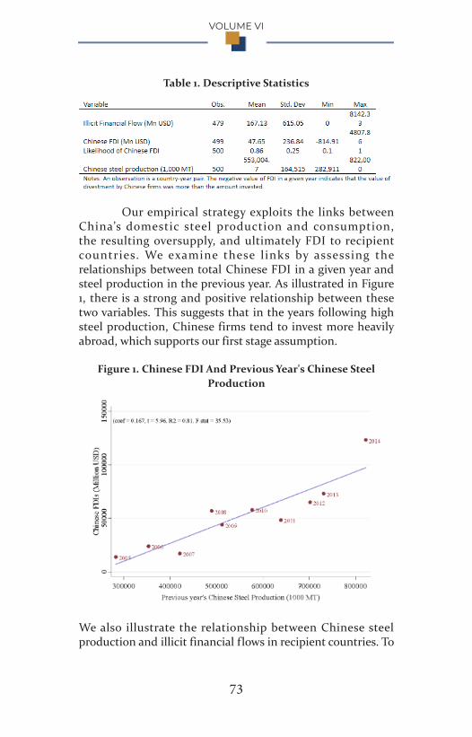
VOLUME VI
73
Table 1. Descriptive Statistics
Our empirical strategy exploits the links between China’s domestic steel production and consumption, the resulting oversupply, and ultimately FDI to recipient countries. We examine these links by assessing the relationships between total Chinese FDI in a given year and steel production in the previous year. As illustrated in Figure 1, there is a strong and positive relationship between these two variables. This suggests that in the years following high steel production, Chinese firms tend to invest more heavily abroad, which supports our first stage assumption.
Figure 1. Chinese FDI And Previous Year's Chinese Steel Production
We also illustrate the relationship between Chinese steel production and illicit financial flows in recipient countries. To
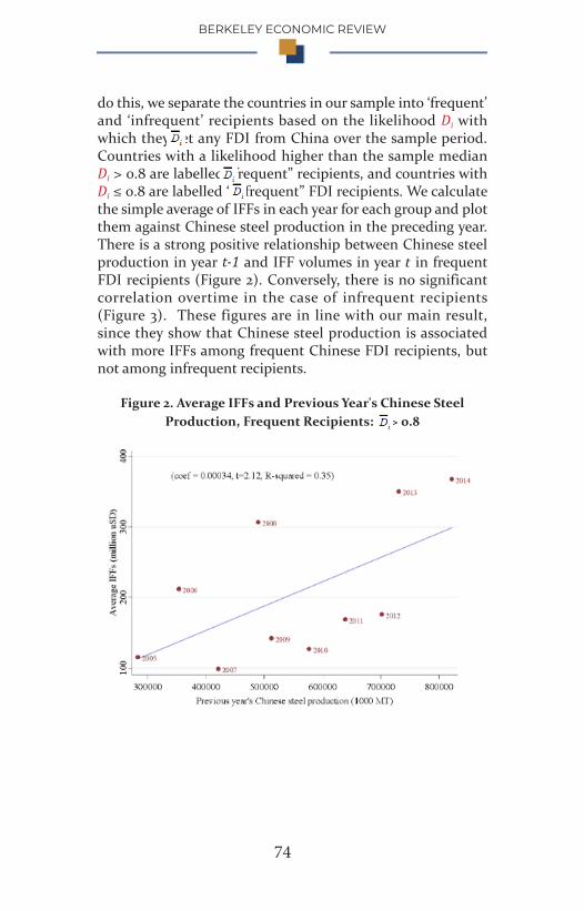
BERKELEY ECONOMIC REVIEW
74
do this, we separate the countries in our sample into ‘frequent’ and ‘infrequent’ recipients based on the likelihood Di with which they get any FDI from China over the sample period. Countries with a likelihood higher than the sample median Di > 0.8 are labelled “frequent” recipients, and countries with Di ≤ 0.8 are labelled “infrequent” FDI recipients. We calculate the simple average of IFFs in each year for each group and plot them against Chinese steel production in the preceding year. There is a strong positive relationship between Chinese steel production in year t-1 and IFF volumes in year t in frequent FDI recipients (Figure 2). Conversely, there is no significant correlation overtime in the case of infrequent recipients (Figure 3). These figures are in line with our main result, since they show that Chinese steel production is associated with more IFFs among frequent Chinese FDI recipients, but not among infrequent recipients.
Figure 2. Average IFFs and Previous Year's Chinese Steel Production, Frequent Recipients: Di > 0.8

VOLUME VI
75
Figure 3. Average IFFs And Previous Year’s Chinese Steel Production, Infrequent Recipients: Di ≤ 0.8
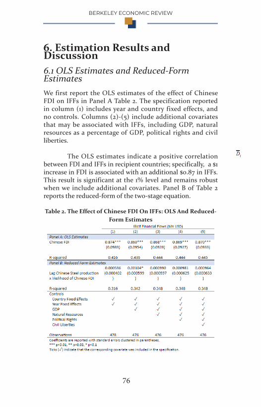
BERKELEY ECONOMIC REVIEW
76
6. Estimation Results and Discussion6.1 OLS Estimates and Reduced-Form EstimatesWe first report the OLS estimates of the effect of Chinese FDI on IFFs in Panel A Table 2. The specification reported in column (1) includes year and country fixed effects, and no controls. Columns (2)-(5) include additional covariates that may be associated with IFFs, including GDP, natural resources as a percentage of GDP, political rights and civil liberties.
The OLS estimates indicate a positive correlation between FDI and IFFs in recipient countries; specifically, a $1 increase in FDI is associated with an additional $0.87 in IFFs. This result is significant at the 1% level and remains robust when we include additional covariates. Panel B of Table 2 reports the reduced-form of the two-stage equation.
Table 2. The Effect of Chinese FDI On IFFs: OLS And Reduced-Form Estimates
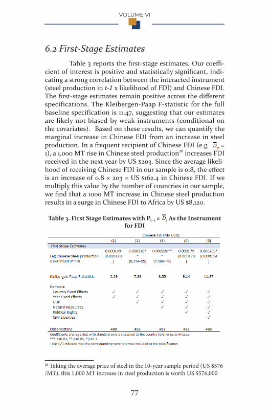
VOLUME VI
77
6.2 First-Stage Estimates Table 3 reports the first-stage estimates. Our coeffi-cient of interest is positive and statistically significant, indi-cating a strong correlation between the interacted instrument (steel production in t-1 x likelihood of FDI) and Chinese FDI. The first-stage estimates remain positive across the different specifications. The Kleibergen-Paap F-statistic for the full baseline specification is 11.47, suggesting that our estimates are likely not biased by weak instruments (conditional on the covariates). Based on these results, we can quantify the marginal increase in Chinese FDI from an increase in steel production. In a frequent recipient of Chinese FDI (e.g Dit = 1), a 1,000 MT rise in Chinese steel production26 increases FDI received in the next year by US $203. Since the average likeli-hood of receiving Chinese FDI in our sample is 0.8, the effect is an increase of 0.8 × 203 = US $162.4 in Chinese FDI. If we multiply this value by the number of countries in our sample, we find that a 1000 MT increase in Chinese steel production results in a surge in Chinese FDI to Africa by US $8,120.
Table 3. First Stage Estimates with Pt−1 × Di As the Instrument for FDI
26 Taking the average price of steel in the 10-year sample period (US $576 /MT), this 1,000 MT increase in steel production is worth US $576,000

BERKELEY ECONOMIC REVIEW
78
6.3 2SLS EstimatesTable 4 reports 2SLS estimates. The estimates indicate that a $1 increase in Chinese FDI increases IFFs in recipient countries by $3.72. The estimates are similar in magnitude and statis-tically significant across different specifications. It is useful to contextualize the magnitude of this estimate within other empirical studies. The United Nations Economic Commis-sion for Africa (UNECA) has conducted its own study of IFFs in Africa and estimated that those flows amount to $30 to $60 billion every year, compared to $19bn received in aid, suggest-ing that as much as 2 to 3 times the amount that flows in is lost to IFFs. A study by Kar (2016) also evaluated the magni-tude of IFFs in comparison to financial inflows in developing countries, including aid, trade f lows and FDI. The author finds that, in 2012, developing nations received $1.3tn in total flows from abroad, compared to $3.3tn in outflows, meaning a three-fold effect. Granted, these studies simply compare in-flows and illicit outflows and do not provide evidence for any causal links. Nonetheless, these figures are helpful in check-ing the relative plausibility of our estimates.
Table 4. 2SLS Regression with Pt-1 x Di As the Instrumental Vari-able
VOLUME VI
79
6.4 Controlling for Lagged Illicit Financial Flows
While our results show a positive causal link between Chinese FDI and illicit financial activity in African countries, a poten-tial concern is that IFFs might be heavily determined by their past level and thus that our estimates do not accurately cap-ture the prior presence of these flows in recipient countries. We therefore report a model that controls for one-year lagged illicit financial f lows. Table 5 shows the estimates that we obtain for the OLS, reduced-form and 2SLS equations. The OLS estimates still show a strong relationship between FDI and IFFs, and the 2SLS show a slightly higher but still positive effect compared to our baseline estimates (4.49 compared to 3.72). However, the first stage estimates are weaker in this case, as shown by the Kleibergen-Paap F-statistic (6.95).
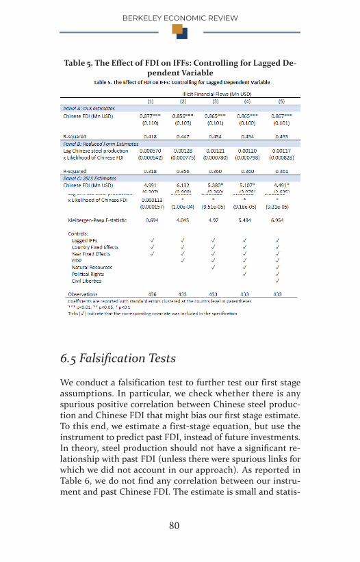
BERKELEY ECONOMIC REVIEW
80
Table 5. The Effect of FDI on IFFs: Controlling for Lagged De-pendent Variable
6.5 Falsification Tests
We conduct a falsification test to further test our first stage assumptions. In particular, we check whether there is any spurious positive correlation between Chinese steel produc-tion and Chinese FDI that might bias our first stage estimate. To this end, we estimate a first-stage equation, but use the instrument to predict past FDI, instead of future investments. In theory, steel production should not have a significant re-lationship with past FDI (unless there were spurious links for which we did not account in our approach). As reported in Table 6, we do not find any correlation between our instru-ment and past Chinese FDI. The estimate is small and statis-
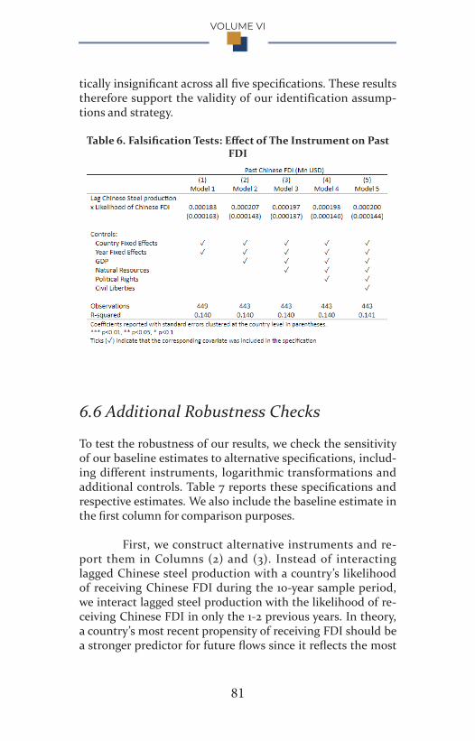
VOLUME VI
81
tically insignificant across all five specifications. These results therefore support the validity of our identification assump-tions and strategy.
Table 6. Falsification Tests: Effect of The Instrument on Past FDI
6.6 Additional Robustness Checks
To test the robustness of our results, we check the sensitivity of our baseline estimates to alternative specifications, includ-ing different instruments, logarithmic transformations and additional controls. Table 7 reports these specifications and respective estimates. We also include the baseline estimate in the first column for comparison purposes.
First, we construct alternative instruments and re-port them in Columns (2) and (3). Instead of interacting lagged Chinese steel production with a country’s likelihood of receiving Chinese FDI during the 10-year sample period, we interact lagged steel production with the likelihood of re-ceiving Chinese FDI in only the 1-2 previous years. In theory, a country’s most recent propensity of receiving FDI should be a stronger predictor for future flows since it reflects the most
BERKELEY ECONOMIC REVIEW
82
up-to-date ties between China and that country. Column (2) interacts lagged steel production with a dummy variable that is 1 if the country received Chinese FDI in the previous year (t-1) and 0 otherwise. Column (3) interacts lagged steel production with the likelihood of positive FDI inf lows in the two previous years (1 if the country received FDI in both years, 0.5 if it received it in one year out of the two, and 0 if it didn’t receive any). The estimates remain positive and sim-ilar in magnitude to our baseline ones, but the first stage is weaker in this case. A major limitation of this strategy is that it reduces the sample period by the number of years we use in constructing the instrument, and we are thus left with less than ten years of data. This then limits the variance within our sample and might weaken our estimates.
Next, we use natural logs of Chinese FDI, IFFs and Chinese steel rather than raw values (column (4)).27 This provides us with proportional rather than linear estimates. We find that a 1% increase in FDI results in an increase in IFFs by 0.2%, a result that is significant at the 1% level. The Kleibergen-Paap F-statistic in this case is 15.92, suggesting a plausible first stage assumption. We also normalize FDI by the populations of the recipient countries (for a measure of dollars of FDI/person) (column 5). The estimate is positive and significant, but the first stage F-statistic is slightly weaker in this case (9.95).
Finally, we test the contemporaneous effect of Chi-nese FDI to understand if the effects of FDI are most prom-inent in the years in which it is received. To this end, we add one-year leads and lags of Chinese FDI in our 2SLS regres-sion. Columns (6) and (7) show that the coefficients for the lag and lead variables respectively are not statistically signifi-cant; nor are the ones for Chinese FDI. These results support the hypothesis that Chinese FDI mostly affects IFFs in the year it is received, i.e. at the same time as the projects are set-up on the ground. It is worth noting that the first-stage esti-mates are weak in these specifications, potentially because 27 IFFs and FDI data include several zero-value observations. To address this in a logarithmic transformation, we add 1 to all values of IFFs, FDI and steel production.
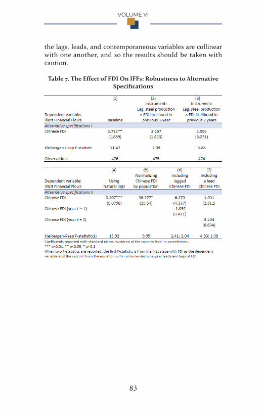
VOLUME VI
83
the lags, leads, and contemporaneous variables are collinear with one another, and so the results should be taken with caution.
Table 7. The Effect of FDI On IFFs: Robustness to Alternative Specifications
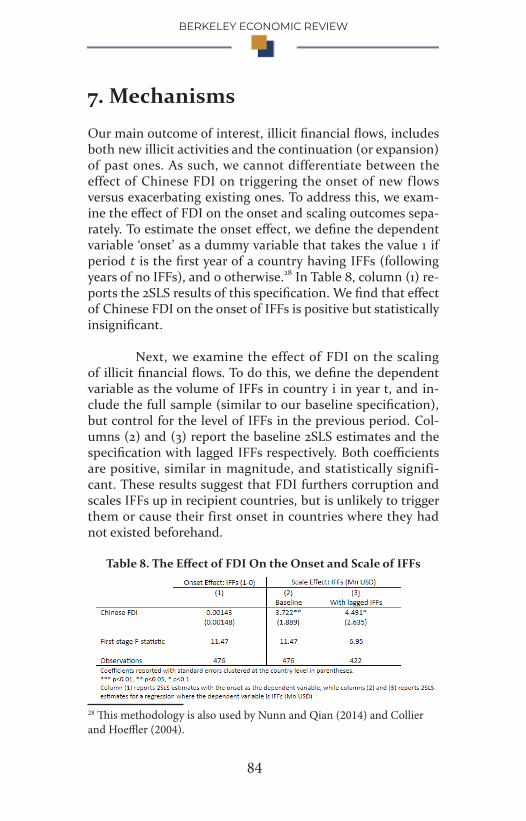
BERKELEY ECONOMIC REVIEW
84
7. Mechanisms
Our main outcome of interest, illicit financial flows, includes both new illicit activities and the continuation (or expansion) of past ones. As such, we cannot differentiate between the effect of Chinese FDI on triggering the onset of new flows versus exacerbating existing ones. To address this, we exam-ine the effect of FDI on the onset and scaling outcomes sepa-rately. To estimate the onset effect, we define the dependent variable ‘onset’ as a dummy variable that takes the value 1 if period t is the first year of a country having IFFs (following years of no IFFs), and 0 otherwise.28 In Table 8, column (1) re-ports the 2SLS results of this specification. We find that effect of Chinese FDI on the onset of IFFs is positive but statistically insignificant.
Next, we examine the effect of FDI on the scaling of illicit financial flows. To do this, we define the dependent variable as the volume of IFFs in country i in year t, and in-clude the full sample (similar to our baseline specification), but control for the level of IFFs in the previous period. Col-umns (2) and (3) report the baseline 2SLS estimates and the specification with lagged IFFs respectively. Both coefficients are positive, similar in magnitude, and statistically signifi-cant. These results suggest that FDI furthers corruption and scales IFFs up in recipient countries, but is unlikely to trigger them or cause their first onset in countries where they had not existed beforehand.
Table 8. The Effect of FDI On the Onset and Scale of IFFs
28 This methodology is also used by Nunn and Qian (2014) and Collier and Hoeffler (2004).
VOLUME VI
85
8. Heterogeneous Effects of Chinese FDI
Finally, we check if the effects of Chinese FDI on IFFs are het-erogeneous across different political and social contexts. To this end, we allow the effect of FDI on IFFs to vary based on the attributes of recipient countries, namely income, natural resource dependence, and the presence of democratic institu-tions. Equation (3) shows the second-stage of our estimation, where Iit refers to the aforementioned country characteris-tics, and the remaining variables remain as in equation (1).
(3)
The country fixed effects in this model absorb the direct effect of the indicator variable Iit on IFFs, and thus the main difference between our previous 2SLS equation and equation (3) is the interaction term FDIit × Iit included in the latter. To establish causality, and following the same logic as the first half of the paper, we instrument for FDIit and (FDIit
× Iit) by using (Pt-1 × Di) and (Pt-1 × Di × Iit) and (Pt-1 × Iit). The first-stage equation therefore becomes:
(4) We focus on factors that other studies linked to the economic performance in developing countries, namely in-come, natural resource dependence, and the quality of polit-ical institutions (Soros 2017; Collier 2007; and Dreher, et al. 2008). We examine these characteristics by constructing Iit as a dummy variable that takes the value 1 if the characteristic in question in country i is greater than the median of the sam-ple. Table 9 reports these estimates and also shows the base-line specification in column (1) for reference. We also report the sum of the coefficients for FDIit × Iit and FDIit, which cap-tures the total effect of FDI for recipient countries that meet the specified criteria.
BERKELEY ECONOMIC REVIEW
86
First, we allow for heterogeneity by income. We mea-sure income using real per capita GDP reported by the World Bank Indicators.29 The estimates (column 2) show that recip-ient countries with high GDP per capita experience less illicit financial activity, potentially because high income is usually associated with strong institutions and established regulatory standards. We note however that while the coefficient of the term FDIit × Iit is negative, the differential effect is imprecise-ly estimated, as shown by a low first stage F-statistic.
Second, we examine whether natural resource en-dowment influences the effect of FDI on illicit activity. We measure natural resource dependence using the percentage of resource rent in GDP.30 On one hand, natural resource depen-dency may reduce the role of FDI in illicit activity by shifting illicit financial f lows towards the agricultural sector rather than foreign projects. However, it could also lead to more IFFs since developing nations have long been shown to suffer a ‘resource curse’, whereby resource wealth increases incentives for illicit rents (Sachs and Warner, 1999). While our estimates (reported in column (3)) seem more in line with the former hypothesis, the standard errors are large, and so our estimates are not entirely reliable.
Finally, we check the differential effect of FDI on IFFs based on democratic institutions. We use the PolityIV data-base31 to determine the democracy level of recipient countries, with scores above 6 (out of 10) indicating democratic leaders and accountable institutions (Column (4)).32 There is no sig-nificant differential effect of FDI received by democracies, relative to more autocratic governments. We note, however, that since our dataset comprises around 450 data points, the heterogeneity tests reduce our sample significantly, and thus affect the precision of the reported estimates. The first stage 29 The mean GDP per capita in our sample is US $2473.03, and the mean percentage of natural resources in GDP is 15.54. We use these thresholds to define our indicator variable Iit30 Reported by the World Bank Indicators31 See Marshall, Monty G., Ted Robert Gurr, and Keith Jaggers. (2016)32 This threshold is the same one used by PolityIV data base to categorize democracies
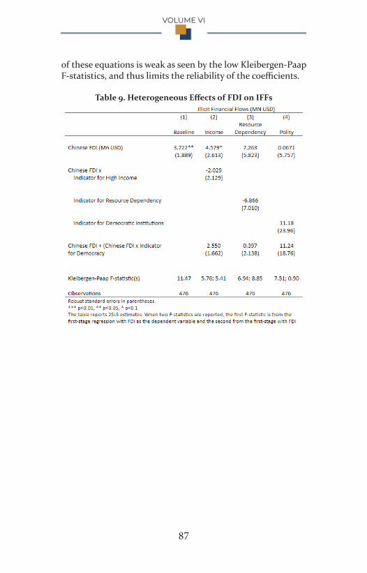
VOLUME VI
87
of these equations is weak as seen by the low Kleibergen-Paap F-statistics, and thus limits the reliability of the coefficients.
Table 9. Heterogeneous Effects of FDI on IFFs

BERKELEY ECONOMIC REVIEW
88
9. Limitations
Our study has a number of limitations related to the nature of the data and the strength of the instrument. For example, the earliest Chinese FDI data is from 2004, and the latest one available is from 2014.33 Prior to this, Beijing reported “China Approved Overseas Investment” data which combined FDI and aid projects, so the data is not comparable. This therefore limits the available data to 10 years and limits the scope of our results. Additionally, our data set does not differentiate between state-owned enterprises and private firms, which might behave differently in foreign markets. Our data is also limited since it only includes macroeconomic variables (such as FDI, GDP and IFFs) but does not provide project-level data, which might reveal industry-specific trends or point toward specific characteristics of Chinese project sites that make IFFs more likely. Moreover, while the first stage of our strategy is strong, it remains imprecisely estimated when we do not include additional covariates. Therefore, the magni-tudes of our estimates should be interpreted with caution.
33 Reported in the 2007 China Statistical Yearbook and the Statistical Bulletin of China's Outward Foreign Direct Investment).
VOLUME VI
89
10. Conclusion
Foreign Direct Investment is an important catalyst of eco-nomic growth in emerging economies. However, critics have argued that FDI, and particularly Chinese-led investment on the African continent, is often associated with inadequate checks and balances, and is therefore an enabler of high-level corruption. This is particularly alarming if we examine the bigger picture – that the African continent loses between $30 and $60 billion to illicit financial flows a year, as reported by the United Nations Economic Commission for Africa. How-ever, there is little to no causal evidence to support these crit-icisms on a large scale.
This study attempted to fill this gap by providing causal evidence of the effect of Chinese FDI on illicit financial flows in recipient countries. The paper uses a new data set by Global Financial Integrity on illicit financial activity in de-veloping countries. Our methodology is also novel in that it uses an instrumental variable for FDI (domestic Chinese steel production interacted with the likelihood of a country being a recipient of Chinese funds). Our findings support the con-cerns advanced by observers and political scientists. Chinese FDI indeed increases IFFs in recipient countries by as much as $3.72 for every additional $1 of FDI, or a 0.2% increase for each 1% rise in FDI. The combined findings of this study all point in the same direction. The OLS, 2SLS and alternative specifications in our robustness tests show a positive and significant effect of Chinese FDI on IFFs and suggest a causal relationship between the two. Moreover, we do not find ev-idence that FDI triggers the onset of illicit activity. Instead, Chinese FDI appears to scale existing flows up. Interestingly, our estimates are consistent with a contemporaneous effect, i.e. that Chinese FDI mostly affects IFFs during the year in which it is received. While we do not find differential effects based on income, resource endowment, or political insti-tutions, our findings nonetheless indicate an adverse effect of FDI on average. It is important to note, however, that our 2SLS estimates of the effect Chinese FDI on IFFs are larger than the OLS estimates. This is potentially due to a selective
BERKELEY ECONOMIC REVIEW
90
targeting of FDI recipients from China’s side. Whether delib-erately or not, Chinese FDI might have gone into countries where its effect on corruption is less adverse.
As for policy implications, since our findings suggest a causal relationship between Chinese FDI and IFFs in re-cipient countries, a potential recommendation would be to strengthen regulatory checks on Chinese-led projects, partic-ularly in recipient countries with a history of large IFFs. This includes the responsibility of recipient countries and China’s own requirements for its firms investing abroad. That being said, while these findings raise concerns around the regula-tions around FDI, they do not necessarily negate the existing evidence on the positive effects of FDI on job creation, skill development and income growth.
This study also suggests several avenues for further research. One of them is to exploit micro-level (e.g. proj-ect-level) data to disentangle the heterogeneity between the effect of FDI on IFFs in different industries and project-types. This would provide a more granular picture of the link be-tween project set-ups and subsequent IFFs and would thus inform sub-government level policies. Overall, the study of FDI provides important evidence of the impact of private-sec-tor activities in developing nations, and will hopefully guide the design of both FDI projects and regulations governing them in the future.
VOLUME VI
91
12. References African Development Bank (2013). “New AfDB-GFI Joint
Report: Africa a Net Creditor to the Rest of the
World”, 5 May 2013, http://www.afdb.org/en/news-
and-events/article/new-afdbgfi-joint-report-africa-a-
net-creditor-to-the-rest-of-the-world-11856/
Baker, R., Clough, C., Kar, D., LeBlanc, B. and Simmons, J.
(2014). Hiding in Plain Sight: Trade Misinvoicing and
the Impact of Revenue Loss in Ghana, Kenya,
Mozambique, Tanzania, and Uganda: 2002-2011.
Washington DC: Global Financial Integrity
Boyce, James K., and Léonce Ndikumana (2012). Capital
Flight from Sub-Saharan African Countries: Updated
Estimates, 1970–2010. PERI Research Report.
Amherst, MA: University of Massachusetts Amherst,
Political Economy Research Institute.
Buckley, P.J. (2004b) ‘The role of China in the global strategy
of multinational enterprises’, Journal of Chinese
Economic and Business Studies 2(1): 1-25.
China-Africa Economic and Trade Cooperation (2013).
English.gov.cn. from http://ke.china-embassy.org/
eng/zfgx/t1090838.htm
http://english.gov.cn/state_council/
ministries/2017/05/11/content_281475652349490.htm
Choe, J. Il. (2003). Do Foreign Direct Investment and Gross
Domestic Investment Promote Economic Growth?
Review of Development Economics, 7(1), 44-57.
Chowdhury, A., & Mavrotas, G. (2006). FDI and Growth:
What Causes What? World Economy, 29(1), 9-19.
BERKELEY ECONOMIC REVIEW
92
Collier, Paul, and Anke Hoeffler. (2004) "Greed and Grievance
in Civil War." Oxford Economic Papers 56, no. 4: 563-
95. http://www.jstor.org/stable/3488799.
Collier, Paul and Benedict Goderis (2007). “Commodity
Prices, Growth, and the Natural Resource Curse:
Reconciling a Conundrum.” Oxford University
Typescript.
"Data: Chinese And American FDI To Africa". (2018). China
Africa Research Initiative. http://www.sais-cari.org/
data-chinese-and-american-fdi-to-africa/.
De Carvalho, A. (2017). Steel Market Development Q2 2017.
Oecd.org. from https://www.oecd.org/industry/ind/
steel-market-developments-2017Q2.pdf
Dreher, A et. Al (2016) “Aid on Demand: African Leaders
and the Geography of China’s Foreign Assistance”
AidData, Working Paper 3.
Dreher, A., Kotsogiannis, C., & McCorriston, S. (2008). How
do institutions affect corruption and the shadow
economy? International Tax and Public Finance,
16(6), 773-796. http://dx.doi.org/10.1007/s10797-008-
9089-5
Earnst and Young (2017). Connectivity Redefined: EY’s
Attractiveness Program Africa. http://www.ey.com/
Publication/vwLUAssets/ey-attractiveness-program-
africa-2017-connectivity-redefined/$FILE/ey-
attractiveness-program-africa-2017-connectivity-
redefined.pdf
Freedom House (2018), Aggregate Category and Subcategory
Scores 2003-2018 https://freedomhouse.org/report-
types/freedom-world

VOLUME VI
93
Global Financial Integrity (GFI). (2017). Illicit Financial Flows
to and from Developing Countries: 2005-2014.
http://www.gfintegrity.org/report/illicit-financial-
flows-to-and-from-developing-countries-2005-2014/
Information Office of the State Council. (2013). “China-Africa
Economic and Trade Cooperation (2013).”
Information Office of the State Council.
http://english.gov.cn/archive/white_
paper/2014/08/23/content_281474982986536.htm
Isaksson, A. and Kotsadam, A. (2016). Chinese aid and local
corruption. AidData, [online] Working Paper 33.
http://docs.aiddata.org/ad4/pdfs/wps33_chinese_
aid_and_local_corruption.pdf
Jayaram, Kassiri, and Sun (2017). The closest look yet at
Chinese economic engagement in Africa. Mckinsey.
http://www.mckinsey.com/global-themes/middle-
east-and-africa/the-closest-look-yet-at-chinese-
economic-engagement-in-africa
Kaplinsky, R., McCormick, D. and M. Morris (2007) “The
Impact of China on Sub-Saharan Africa”, IDS
Working Paper no. 291, Institute of Development
Studies at the University of Sussex Brighton.
Kar, D. and Cartwright-Smith, D. (2010). Illicit financial flows
from Africa: Hidden resource for development.
Washington DC: Global Financial Integrity
Kar, D (2016). "New Report on Unrecorded Capital Flight
Finds Developing Countries Are Net-Creditors to The
Rest Of The World" Global Financial Integrity.
http://www.gfintegrity.org/press-release/new-
report-on-unrecorded-capital-flight-finds-
BERKELEY ECONOMIC REVIEW
94
developing-countries-are-net-creditors-to-the-rest-
of-the-world/.
Kennan, Patrick J. (2009) Curse or Cure - China, Africa, and
the Effects of Unconditional Wealth, 27 Berkeley J.
Int'l Law. 84 (2009). https://doi.org/10.15779/
Z38007X
Lang, Bertram. 2017. "Engaging China in The Fight Against
Transnational Bribery: “Operation Skynet” As A New
Opportunity for OECD Countries". Oecd.Org.
https://www.oecd.org/cleangovbiz/Integrity-Forum-
2017-Lang-China-transnational-bribery.pdf.
Marsh, Jenni. 2018. "How A Hong Kong Bribery Case Exposes
China's Corruption Problem in Africa". CNN. https://
edition.cnn.com/2018/02/09/world/patrick-ho-
corruption-china-africa/index.html.
Marshall, Monty G., Ted Robert Gurr, and Keith Jaggers.
(2016). POLITY IV PROJECT Annual Time-Series,
1800-2016, 1800-2015 Dataset Users’ Manual. Centre
for Systemic Peace. http://www.systemicpeace.org/
inscrdata.html
McDonald, D. C. (1985). Trade Data Discrepancies and the
Incentive to Smuggle: An Empirical Analysis.
International Monetary Fund Staff Papers, 32 (4),
668-692.
Meyersson, E., Miquel, G. and Qian, N. (2008). “The Rise
of China and the Natural Resource Curse in Africa”
London School of Economics, [online] Working
Paper. Available at: http://personal.lse.ac.uk/padro/
older-working-papers/
meyersonpadroqian_20080407_all.pdf.
VOLUME VI
95
Morck, Randall, Bernard Yeung, and Minyuan Zhao (2008).
"Perspectives on China's Outward Foreign Direct
Investment." Journal of International Business
Studies 39, no. 3: 337-50. http://www.jstor.org.
libproxy1.nus.edu.sg/stable/25483271.
Naím, M (2007) “Rogue Aid”, Foreign Policy, No. 159, March/
April 2007.
Ndikumana, L. and Boyce, J. K. (2010). Measurement of
capital flight: Methodology and results for sub-
Saharan African countries. African Development
Review, 22 (4), 471-481.
Nunn, Nathan, and Nancy Qian. (2014) "US Food Aid and
Civil Conflict." The American Economic Review 104,
no. 6 (2014): 1630-666. http://www.jstor.org/
stable/42920861.
OECD Convention On Combating Bribery Of Foreign Public
Officials In International Business Transactions -
OECD". (2009). Oecd.Org.
Pehnelt, G. (2007) “The Political Economy of China’s Aid
Policy in Africa”, Jena Economic Research Papers no.
051. University of Jena, Germany
Sachs, Jeffrey D. and Andrew M. Warner. (1999) "The Big
Rush, Natural Resource Booms And Growth," Journal
of Development Economics, v59(1,Jun), 43-76.
Soros, George. Escaping the Resource Curse. Edited by
HUMPHREYS MACARTAN, SACHS JEFFREY D.,
and STIGLITZ JOSEPH E. Columbia University Press,
2007. http://www.jstor.org/stable/10.7312/
hump14196.
"Spotlight on Foreign Corrupt Practices Act". 2018. Sec.Gov.
BERKELEY ECONOMIC REVIEW
96
https://www.sec.gov/spotlight/fcpa/fcpa-cases.
shtml.
Spegele, Brian, and John W. Miller. 2016. China Continues
to Prop Up Its Ailing Factories, Adding to Global
Glut. Wall Street Journal.
The World Bank. 2018. World Development Indicators.
Washington, D.C.: The World Bank. (Indicators :
Natural Resources Rents and GDP per capita) http://
data.worldbank.org/data-catalog/world-
development-indicators
Tull, Denis M. 2006. China’s Engagement in Africa: Scope,
Significance and Consequences. Journal of Modern
African Studies 44, 3: 459-479.
United Nations Conference on Trade and Development. (2018)
“UNCTAD Annual Report.” New York :United
Nations, n.d.
United Nations Economic Commission for Africa (UNECA),
Report of the High Level Panel on Illicit Financial
Flows from Africa (2015) https://www.uneca.org/
sites/default/files/PublicationFiles/iff_main_
report_26feb_en.pdf
Vu, T.B., Gangnes, B., & Noy, I. (2008). Is foreign direct
investment good for growth? Evidence from sectoral
analysis of China and Vietnam. Journal of the Asia
Pacific Economy, 13(4), 542-562.
Steel Statistical Yearbook (2016), World Steel Association.
https://www.worldsteel.org/en/dam/
jcr:37ad1117-fefc-4df3-b84f-6295478ae460/
Steel+Statistical+Yearbook+2016.pdf
"World Investment Report 2017". 2017. United Nations

VOLUME VI
97
Conference on Trade and Development Unctad.Org.
http://unctad.org/en/PublicationsLibrary/wir2017_
en.pdf.
Yu, H., & Yang, M. (2010). China’s Steel production: An
update. Eai.nus.edu.sg., from http://www.eai.nus.
edu.sg/publications/files/BB501.pdf
Zheng, Jinghai, Arne Bigsten, and Angang Hu. (2009). Can
China’s Growth be Sustained? A Productivity
Perspective. World Development 37, 4: 874-888
BERKELEY ECONOMIC REVIEW
98
Real Exchange Rate Volatility and Economic Growth:
A Panel Data InvestigationFederico Pessina
University of Warwick
Abstract
The study aims to investigate the impact of Real Effective Exchange Rate (REER) volatility on economic growth for a set of 33 developed and developing economies, using panel dataset ranging from 1970 to 2016. Stemming from a precise measure for exchange rate volatility, results of various Fixed Effects and System GMM models suggest that increased (decreased) REER volatility, controlling for trade and misalignment and contingent on diverse model specifications, leads to a negative (positive) effect on economic growth for developing countries. A relationship cannot be ascertained for developed countries. In addition, a significant impact of the REER level and its interaction with volatility is found, while neither a significant interaction of volatility with trade nor terms of trade shocks is found.
Acknowledgements
I would like to thank my supervisor Jingyi Mao for her excep-tional help, insights and constant support.
VOLUME VI
99
TABLE OF CONTENTSI. Introduction .............................................................. 100
II. Exchange Rate Volatility and Economic Growth ................................................................................................ 102
III. Modelling REER Volatility ................................... 106
IV. Empirical Strategy ................................................. 109
V. Data Source and Descriptive Statistics ................. 113 Data Sources .................................................... 113 Descriptive Statistics ...................................... 113
VI. Empirical Results ................................................... 116 Analysis of the Results ................................... 116 Robustnesss of the Estimators ...................... 118
VII. Conclusion, Limitations and Extensions .......... 120 Appendix ......................................................... 122
A1. Country Data ........................................................ 122 A2. Definition of Variables ......................................... 123A3. Tests on Panel Data .............................................. 124A4. Correlation Between Explanatory Variables ..... 125A5. Diagnostic Testing ................................................ 126A6. Results of Main Regressions ................................ 127
Bibliography ................................................................. 128

BERKELEY ECONOMIC REVIEW
100
I. IntroductionThe choice of exchange rate regimes is one of the most debat-ed variables in macroeconomic policy. Exchange rate regimes, volatility and misalignment of the exchange rate are inherent-ly interlinked.1 A growing body of literature, focused in partic-ular on Real Exchange Rate (RER) misalignment, has devel-oped to investigate their effects on economic growth.2 While misalignment is a critical aspect, I argue that RER volatility, which causes uncertainty in trade, is equally impactful given its potential effects on growth.
Theoretical and empirical literature regarding the ad-vantages and disadvantages of different regimes is generally inconclusive, as the proponents of diverse systems indicate contrasting effects of volatility on macroeconomic variables. In the same manner, literature has been unable to ascertain a relationship between volatility and growth or its components. 3As noted by Vieira et al. (2013), utilisation of standard devia-tion (s.d.) as a measure of volatility implies clear limitations, which will be explored later.4 Inconsistent methodologies in RER estimation have also led to diverse results. Literature on exchange rate misalignment has typically been a divisive is-sue, due to measurement inaccuracy caused by the necessity of estimating an equilibrium exchange rate and the contrast between macroeconomic instability and outward-oriented growth strategies, both potentially caused by misalignment in the exchange rate.
The motivation of this paper is to complement these studies with an investigation of the effects of Real Effective Exchange Rate (REER) volatility on economic growth and its components. I draw from previous results the model specifica-tion and control variables. In addition, this paper strives to go beyond previous literature in a variety of ways. Firstly, I utilize 1 Eichengreen, 20072 Defined as the difference between observed exchange rate and the long-run equilibrium exchange rate (Eichengreen, 2007; Levy-Yeyati & Sturzenegger, 2002).3 Eichengreen, 20074 Vieira et al., 2013

VOLUME VI
101
REER instead of RER, a broad measure of the country’s com-petitiveness. I use monthly figures instead of annual, which are calculated with a consistent methodology for the whole panel, implying a higher level of precision when modelling annual REER volatility. Secondly, I overcome the limitations of using s.d as measure of volatility by modelling it with a Generalized Autoregressive Conditional Heteroskedasticity (GARCH) pro-cess. Thirdly, I focus on the relationship between REER volatil-ity, trade and terms of trade (TOT). By differentiating whether the economy is developing or not, I investigate if the impact of volatility is more pronounced if trade represents a larger share of the economy and if the country is experiencing any TOT shocks.
The paper is based on a panel dataset ranging from 1970 to 2016 for 33 different countries, therefore concentrating on the post-Bretton Woods period. Stemming from a precise measure for exchange rate volatility, results of various Fixed Ef-fects, Between-Within and System GMM Models suggest that increased (decreased) REER volatility, controlling for trade and misalignment and contingent on diverse model specifica-tions, leads to a negative (positive) effect on economic growth for developing countries. A relationship cannot be ascertained for developed countries. A significant impact of the REER level on volatility is found, while no significant interaction of vola-tility neither with trade nor TOT shocks is found.

BERKELEY ECONOMIC REVIEW
102
II. Exchange Rate Volatility and Economic GrowthFollowing the fall of the Bretton-Woods system, exchange rate volatility has become a topic of interest given its potentially critical implications for economic policy. Theoretical and em-pirical literature have attempted to investigate the relation-ship between exchange rate volatility and economic growth, augmenting it with further research regarding the effect of volatility on other macroeconomic indicators such as trade and investment, among others. Results of both theoretical and empirical studies have been inconclusive from contrast-ing results. As noted by Eichengreen (2007), these disagree-ments are generally caused by diverse model specifications and control variables, high dependency on the sample period considered and inconsistent and simplistic methodologies when measuring exchange rate volatility.5 I will focus on lit-erature regarding economic growth that is directly relevant to my paper.
Levy-Yeyati & Sturzenegger (2002) indicate why the relationship between growth and exchange rate volatility has traditionally been disregarded by economists due to the classi-cal money neutrality argument-- nominal variables do not af-fect the long-run equilibrium growth of an economy.6 Howev-er, it is widely accepted that the relationship described above is contingent upon the adopted type of exchange rate regime.7
The debate on the advantages and disadvantages of different exchange rate regimes provides useful insights. Ad-vocates of flexible exchange rates argue that, in cases of real shocks on the economy, flexibility facilitates the adjustment process.8 Ghosh et al. argues that fixed exchange rates may create RER misalignment, leading to erroneous price signals and thus inefficient allocation of resources.9 Alternatively, 5 Eichengreen, 2007.6 Levy-Yeyati and Sturzenegger, 20027 Eichengreen, 2007.8 Levy-Yeyati and Edwards, 2004; Friedman, 19539 Ghosh et al.
VOLUME VI
103
supporters of fixed exchange rates suggest that the stability of the regime promotes trade and investment. This is through a decrease in uncertainty of prices and real interest rates that firms face that improve the efficiency of price mechanisms on the international scale and will incentivise economic growth.10
Similarly, empirical literature has been inconclusive. For example, Ghosh (1997) analyzed the links between ex-change rate regimes, inflation and growth utilising data on 136 countries over a period of 30 years.11 The study did not find any statistically significant effect of RER volatility on econom-ic growth, but highlighted the importance of controlling for trade and investment when isolating the effects of exchange rate stability on growth. Flexible exchange rates are subject to market forces, theoretically making misalignment less likely, and enhancing the development of export industries that due to stronger competition are associated with higher productiv-ity growth. This paper’s focus on the nominal exchange rate, while aiming to assess changes in long-run economic growth, has been criticised.12
Developing countries may have different priorities when assessing exchange rates. Bleaney & Greenaway (2001) investigated the impact of RER volatility on investment and growth on a panel of 14 sub-Saharan African countries over 1980-1995. They found a significant negative effect on invest-ment but not on economic growth. This paper’s emphasis on developing countries provides useful insights. These develop-ing countries’ dependence on the export of primary products is based on the idea that RER volatility should particularly af-fect economies relying on specialisation in primary products.
Vieira et al. (2013) investigated the impact of RER vol-atility on long-run economic growth for a set of 82 advanced and developing economies, using a panel dataset ranging from 1970 to 2009. They found a significant negative impact of RER on long-run economic growth, even when controlling for country-specific idiosyncrasies. Another interesting result 10 Mundell, 1973; De Grauwe, 199811 Ghosh 199712 Eichengreen, 2007
BERKELEY ECONOMIC REVIEW
104
is when including volatility, neither level of exchange rate nor the misalignment is statistically significant. The authors sug-gest that pursuing a stable exchange rate may be a better strat-egy than exchange rate misalignment when aiming for long-run economic growth. This conclusion ties with the issues in literature regarding exchange rate misalignment briefly high-lighted in Section I. Similarly, Dollar (1992) focused on 95 de-veloping economies, and found a negative impact of exchange rate volatility on economic growth.13 Dollar included degree of openness as control variable, finding a relationship between it and the impact of volatility on growth.14
Literature has aimed to investigate the relation by looking at the components of economic growth, in particular trade. Nevertheless, no conclusive evidence has been found on either theoretical or empirical level.15 While exchange rates movements are assumed to be random in the short run, lit-erature recognises that RER does depend on macroeconomic variables in the medium and long run. TOT shocks may drive RER changes, as changes in export and/or import prices will affect nominal exchange rates, inflation and trade.16
Overall, Eichengreen (2007) provides an insightful summary of literature by arguing that while the empirical re-sults have not been conclusive, ensuring a stable, competitive and aligned RER may not directly cause long-run economic growth but will allow a country the possibility of exploring their economic potential thanks to, amongst other reasons, reduced uncertainty and higher competitiveness.17
In my paper, I aim to build upon and fill gaps in the literature addressed above. As mentioned in the introduction, this paper tackles several criticisms of the papers reviewed. Conflicting empirical results are caused by contrasting model specifications, high dependency on the sample period con-
13 Dollar, 199214 Ibid15 Vieira et al., 2013; Franke, 1991; Peree and Steinherr, 198916 Coudert et al., 200817 Eichengreen, 2007
VOLUME VI
105
sidered and naïve volatility measures.18 Following Vieira et al. (2013) and Ghosh (1997), the model will be based upon the key macroeconomic indicators and components of GDP. In addition, I utilize trade as a proxy for degree of openness and investigate its relationship with exchange rate volatility, hypothesising that the impacts of volatility increase together with trade as a share of GDP. TOT has typically been disre-garded in the RER-volatility literature. The paper posits a larg-er impact of volatility when the economy is experiencing large TOT shocks, which are assumed to be exogenous, a common assumption in literature. The paper19 will focus on RER and disregard its nomi-nal counterpart in an attempt to isolate its effects on economic growth. In contrast to Vieira et al. (2013), economic growth will not be modelled around 5-year averages. The model will in-stead be augmented with lagged trade and other indicators, as further investigation of the interaction between trade and vol-atility, as found by Dollar (1992). To conclude, the use of con-sistent methodology when calculating REER and its volatility, together with the focus on the post-Bretton Woods period and the inclusion of a large number of countries, aims to reduce differences between papers, leading to comparable results and higher external validity.
18 Ibid19 Pryor, 1966
BERKELEY ECONOMIC REVIEW
106
III. Modelling REER VolatilityIn this paper, I will utilise REER instead of RER. REER mea-sures the “development of the real value of the country’s cur-rency against the basket of the trading partners of the coun-try”.20 Alternatively, the REER can be defined as the average of the bilateral RER between the country in question and its trading partners, weighted by the respective trade shares of each partner.21 Intuitively, the advantages of REER are clear. Changes in REER provide useful insights for this analysis by indicating the equilibrium value of the currency. This permits us to estimate, albeit simplistically, the level of misalignment and changes in competitiveness of the whole economy, driv-en by either change in exchanges rates or in relative inflation (price or cost competitiveness). REER permits the isolation of the competitiveness of the single country, reducing the noise of the other countries.22
This paper models REER volatility using the dataset “Real Effective Exchange Rates for 178 Countries” developed by Bruegel. The dataset includes both annual and monthly data for a large number of countries. I will utilise monthly REER data from 1970 to 2016 for 33 countries (Appendix 1).
Modelling REER volatility is one of the causes of con-trasting results in literature.23 A contribution of this paper is to use REER calculated with consistent methodology and utilise an innovative measure for volatility coherent with the papers reviewed previously.
20 Bruegel, 201721 IMF, 200722 REER permits us to average out external shocks in the RER, and isolate the competitiveness of Country A.23 Eichengreen, 2007; Siregar and Rajan, 2004
VOLUME VI
107
and Stwi is the nominal bilateral exchange rate betwen the
country under study and country iand wi is the weight associated to country i
Literature has modelled volatility through s.d. by looking at how the exchange rate fluctuates around its mean overtime.24 However, utilising s.d. as measure of volatility is approximate. Firstly, s.d. has a skewed distribution. Secondly, s.d. doesn’t capture the information in the previous periods.25 To an ex-tent, exchange rates are determined by a random process. Thus utilising s.d. leads to ignoring the level of volatility in the previous period, implying that volatility in one period is unaffected by volatility in the previous one.
The paper proceeds by utilising GARCH process, de-veloped by Bollerslev (1986).26 As noted by McKenzie (1999), exchange rates best follow the GARCH process because GARCH, as compared to ARCH, captures the past values and thus permits higher accuracy. I model the variance wt follow-ing a GARCH (1, 1) process on the monthly REER data, for each country, from 1970 to 2016.
The method presents several advantages compared to SD. As mentioned, I am able to capture the effects of volatility of one period on the following one, differentiating between the random and the predictable elements of the exchange rate determination process.27 To conclude, variance is condition-al on the past values and better reflects how volatility is per-ceived by agents.
After obtaining monthly figures for REER volatility, I averaged these numbers to obtain annual volatility figures 24 Schnabl, 200725 Jansen, 198926 Technique first proposed by Engle (1982).27 Ebaidalla, 2013; Arize et al., 2000

BERKELEY ECONOMIC REVIEW
108
for each country from 1970 to 2016. This was done to match the availability of data for macroeconomic indicators.The final output included 1551 observations in total. Descriptive statis-tics are shown in Table 2.
VOLUME VI
109
IV. Empirical StrategyThe aim of this paper is to estimate the effect of REER volatili-ty on economic growth, starting with this initial model:
The choice of control variables follows growth litera-ture and the papers previously reviewed.28 Trade and govern-ment expenditure are denoted as share of GDP. Theoretical literature suggests that inflation may have negative effect on GDP growth due to distortion in price signals as government expenditure is ambiguous. Keynesian Economists argue that government expenditure may increase aggregate demand, while others remind of its crowding-out effect, which leads to lower investment and growth in the long run. Trade is ex-pected to increase GDP growth. Inflation is used as a proxy for macroeconomic stability, while trade represents degree of openness. In conclusion, developing and developed countries will be analyzed separately,29 leading to more insightful re-sults, and potentially limiting endogeneity issues by analysing countries with similar macroeconomic conditions together.
Further models include:1) TOT Shocks, an interaction variable between REER vola-tility, trade and TOT shocks. The paper hypothesizes that the impact of volatility may be different when the country is expe-riencing TOT shocks because they drive RER and control for the importance of trade in the economy. A separate interac-tion variable between trade and REER volatility is investigat-ed, hypothesising that impact on growth is larger when trade represents a larger share of GDP.
28 Eichengreen, 2007; Vieira et al., 201329 See Appendix 1
BERKELEY ECONOMIC REVIEW
110
2) Interaction variables between volatility and GDP per capita as literature suggests that the higher the GDP, the lower the GDP growth. Thus, I control for the variable and investigate any additional effects of volatility.
3) Dummy variables to control for possible regional differenc-es.
4) I also posit whether lagged independent variables such as government expenditure and trade may explain variation in GDP Growth. Given that I am looking at annual data, theo-retical literature suggests that government expenditure may have a multiplier effect. While this is not the aim of the paper, including such terms may be insightful.
5) Diverse functional forms, such as including lagged or squared terms of the independent variable REER volatility.
6) REER misalignment from its equilibrium value.
The model proposed clearly holds endogeneity issues, where some of the variables are determined within the mod-el. One form of endogeneity present is omitted variable bias, inherent to the macroeconomic nature of the model indicated by the existence of inconclusive empirical literature. Omitted variables leads to OLS bias, which implies larger coefficients and lower s.e. for the variables included in the model and thus wrongful conclusions. In this case, the direction of the bias on coefficients is ambiguous.
Firstly, the paper attempts to reduce the bias by es-timating various fixed effects models. Fixed Effects exploits within-group variation. The model involves controlling for the average difference across the countries in any observable/unobservable predictors that are assumed to be time-invari-ant. Therefore, threat of omitted variable bias is reduced. As a price, between- group variation is lost. The paper’s main vari-ables of interest are not time-invariant; thus, the model is use-ful. Choice of Fixed Effects model rests upon data consistent with the theory and assumptions needed to implement it. In
VOLUME VI
111
addition, Hausman tests confirm its suitability.30
Tests are implemented that confirm the presence of autocorrelation, cross-sectional dependence and heterosce-dasticity. The presence of these factors was highly predictable given the nature of the data and variables utilised. Dependent variables may be affected by unexpected variation or shocks. The model thus controls for time-fixed effects, further reduc-ing omitted variable bias and cross-sectional dependence. 31Following the tests, I utilize Driscoll and Kray errors.32
Secondly, I estimate various within-between effects model in an attempt to investigate continent dummies, as these variables are time invariant and cannot be discerned in the fixed-effects model and between-group variation. As men-tioned, results from the Fixed Effects model are assumed to be more robust to endogeneity issues.
Thirdly, the paper investigates dynamic panel data models through system Generalised Method of Moments (GMM), developed by Arellano-Bover (1995) and Blun-dell-Bond (1998), as a further potential solution to endogene-ity issue. In this technique, I utilise lagged levels differences of the endogenous variables as instruments for the regression in differences in levels, together with the already-specified exog-enous instruments.33
Two empirical methods will be employed to reduce the number of instruments. Firstly, the collapse option of the command xtabond2 will be used. Secondly, restrictive lag lim-its will be imposed. An excessive number of instruments would overfit the model, leading to wrongful conclusions and a still present endogeneity issue.34 Time- fixed effects (year-dum-mies) are included to reduce autocorrelation that is logical-ly present in macroeconomic data and mitigate the effects of any trends, although none have been discerned through data 30 See Appendix 331 See Appendix 332 Driscoll and Kray, 199733 Vieria et al., 2013; Roodman, 2009a34 Roodman, 2009b; Windmeijer, 2005

BERKELEY ECONOMIC REVIEW
112
inspection. In conclusion, GMM should lead to more robust estimates of the coefficients and permit the investigation of the dynamic relationship between the variables.
VOLUME VI
113
V. Data Sources and Descriptive Statistics
Data Sources
Data for all macroeconomic variables has been taken from World Development Indicators (2017) dataset, developed by the World Bank (National Accounts data). REER data has been taken from the dataset “Real Effective Exchange Rates for 178 Countries” developed by Bruegel (2017).
Descriptive Statistics
Descriptive statistics are reported in Table 1.35 Inspection of the data suggests the existence of an outlier: Bolivia’s inflation with a reported value of 11749%. The paper does not elimi-nate this data point, given the potentially useful information it contains. Logarithmic transformation of variables reduces the effect of the outlier, and a sensitivity analysis is complet-ed to ensure the validity of the results. Overall, the statistics show broad results and diverse countries on the full spectrum of economic development. Detailed information regarding REER volatility has been covered in Section III.
35 Correlation table reported in Appendix 4.
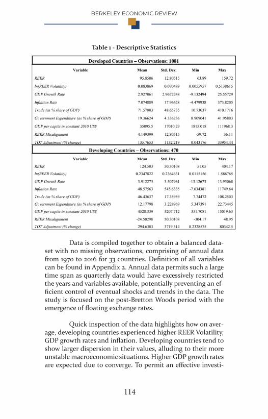
BERKELEY ECONOMIC REVIEW
114
Table 1 - Descriptive Statistics
Data is compiled together to obtain a balanced data-set with no missing observations, comprising of annual data from 1970 to 2016 for 33 countries. Definition of all variables can be found in Appendix 2. Annual data permits such a large time span as quarterly data would have excessively restricted the years and variables available, potentially preventing an ef-ficient control of eventual shocks and trends in the data. The study is focused on the post-Bretton Woods period with the emergence of floating exchange rates.
Quick inspection of the data highlights how on aver-age, developing countries experienced higher REER Volatility, GDP growth rates and inflation. Developing countries tend to show larger dispersion in their values, alluding to their more unstable macroeconomic situations. Higher GDP growth rates are expected due to converge. To permit an effective investi-
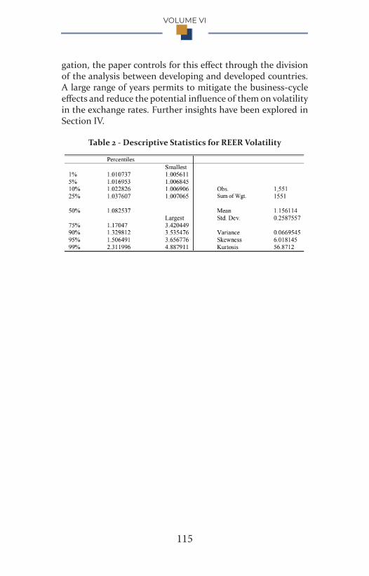
VOLUME VI
115
gation, the paper controls for this effect through the division of the analysis between developing and developed countries. A large range of years permits to mitigate the business-cycle effects and reduce the potential influence of them on volatility in the exchange rates. Further insights have been explored in Section IV.
Table 2 - Descriptive Statistics for REER Volatility
BERKELEY ECONOMIC REVIEW
116
VI. Empirical Results
Analysis of the Results
Table 3 reports the main results. The empirical strategy in-volves estimating the model highlighted in Section IV and then proceed by investigating various interaction variables and control variables, such as the level of REER, the relation-ship between macroeconomic stability and volatility and in-teraction variable between GDP level and volatility. The re-sults are confirmed throughout all models.
All regressions for developing countries indicate sig-nificant, negative coefficients for REER Volatility on economic growth. A significant squared term has been estimated with fixed effects suggesting a concave relationship for developing countries, although successive models were not able to con-firm this. As for developed countries, the results are inconclu-sive. System-GMM indicates that a 1% increase in REER vola-tility leads to around 0.63%fall in GDP growth rate. Because coefficients vary between models a specific value should not be concluded, although the negative direction of the effect has been confirmed by various model specifications.
Progressing through the estimators, it can be seen that macroeconomic controls are central to growth theory. Variables such as government expenditure and inflation are increasingly significant in explaining economic growth. I ex-pect such results due to the estimators increased ability to control for endogeneity, in particular omitted variable bias in this case. Given the limited number of variables used and a general risk of endogeneity when explaining the economy on a macroeconomic scale, the use of more robust estimators is thus essential to ensure appropriate results.

VOLUME VI
117
Table 1 - Empirical Results
Analysis of interaction and control variables provides further insights. No significance is found for the relationship between volatility and trade and TOT shocks, although the paper had hypothesised a potential increased impact of vol-atility. A positive impact of the interaction variable between the level of REER and REER volatility is found for developing countries, while the more robust GMM estimators evidence a further significant impact of the REER level. A similar result is found for developed countries with the GMM estimators, al-
BERKELEY ECONOMIC REVIEW
118
though the study interprets these results as less robust unless its limitations are addressed. This suggests the importance of a REER both competitive and stable. In conclusion, contrasting results have been found for REER misalignment. However, the study though did not investigate misalignment fully, seen as a separate issue from volatility, and thus no concrete conclusion can be inferred.
Regarding the control variables, results show a high degree of robustness with general significance and coefficients of the same sign. Trade, the proxy for degree of openness, has a positive impact on economic growth, with significance al-ways found for developed countries. Inflation, the proxy for macroeconomic stability, instead has a negative impact. Gov-ernment expenditure is, by definition, a divisive issue in liter-ature. Overall, the robustness of the control variables indicate a generally efficient model.
Results of the paper follow results found by papers with similar methodologies, although some stark differenc-es remain. In contrast to Vieira et. al (2013), for example, the REER has found to be generally significant with a positive effect on economic growth. This paper posits that it may be over-simplistic to discard the variable and that instead, most importantly, the coexistence of a competitive and, at the same time, stable REER is a powerful determinant of economic growth. This accords with a general summary of the literature, as noted by Eichengreen (2007).
Robustness of the Estimators
Endogeneity is still present and addressed in limitations and extensions. In contrast to the R2, where high values were not expected due to the macroeconomic nature of the data, the diagnostic testing shows a general validity of the results with normally distributed errors (Appendix 5). The robustness of the control variables is another positive indication. Regarding the dynamic estimators, the inclusion of time-fixed dummies permits the rejection of the AR(2) test and highlights no prob-

VOLUME VI
119
lems of second-order autocorrelation. The Hansen over-iden-tifications tests are generally positive, suggesting the validity of the instruments. In some models I have an instrument-pro-liferation problem, caused by limitations in the data.
BERKELEY ECONOMIC REVIEW
120
VII. Conclusion, Limitations and ExtensionsLiterature has not reached a consensus regarding the role of REER or RER volatility on economic growth. This paper aimed to provide further evidence through the use of a consistent and innovative methodology to measure volatility, and an in-vestigation of the interaction of volatility with trade and TOT shocks. This study is an empirical investigation of the rela-tionship between REER volatility and economic growth on a panel dataset of 33 countries from 1970 to 2016. Overall, after controlling for endogeneity and country-specific characteris-tics through Fixed Effects and GMM estimators, results indi-cate the existence of a negative impact of REER volatility on economic growth for developing countries, while no effect is evidenced for developed countries. No significance is found for the effect of TOT shocks and degree of openness on the im-pact of volatility on economic growth, although a significant positive effect of the level of REER is found.
Results confirm the attention that exchange rates have been given by literature. The choice of exchange rate regime has been a critical decision of governments and policymak-ers when attempting to promote prolonged and sustainable economic growth. The results thus suggest That policy-wise, maintaining low REER volatility and a competitive REER, should be beneficial for economic growth in the case of de-veloping countries. Advising on the choice of an exchange rate regime is beyond the scope of the study. While a fixed regime may, by definition, have the lowest volatility, it may not permit the existence of a competitive REER or be unsustainable, thus being overall detrimental. Managed floating exchange rate, for example, may be a viable alternative.
The limitations of the study stem primarily from the data. In the data collection process, there was a trade-off be-tween the inclusion of countries and variables with missing observations, or their exclusion in order to maintain a bal-anced panel data. The study has followed the second road.

VOLUME VI
121
Therefore, a possible extension of the research is the inclu-sion of new variables and countries. In such a case, in order to maintain a balanced panel dataset, the time range will be much more limited. However, if the time range is reduced, quarterly data could be used, which may evidence short-run dynamics and shocks which are lost on an annual scale or, alternatively, control more effectively for business cycle and trends in GDP growth. A second limitation due to sample size regards the methodology, where this paper was unable to utilise the more efficient two-style estimator, which gives asymptotic efficien-cy for system GMM. Thirdly, the channels through which vola-tility affects economic growth are not modelled. A large degree of endogeneity is still present.
Therefore, further research should aim to explore these limitations and most importantly, investigate the rea-sons why contrasting results have been found between devel-oping and developed countries. Identification of the chan-nels through which exchange rate volatility affects economic growth may suggest the causes of such findings. In addition, these channels may indicate more effective policy recom-mendations. Secondly, identifying the source of REER vola-tility could provide an insightful analysis in the dynamics of the relationship explored by this paper. Thirdly, the potential inclusion of capital flows, current account, inflation differen-tials and interest rates may highlight the flow of capital across countries and enhance the terms-of-trade analysis of this pa-per which have been inconclusive.
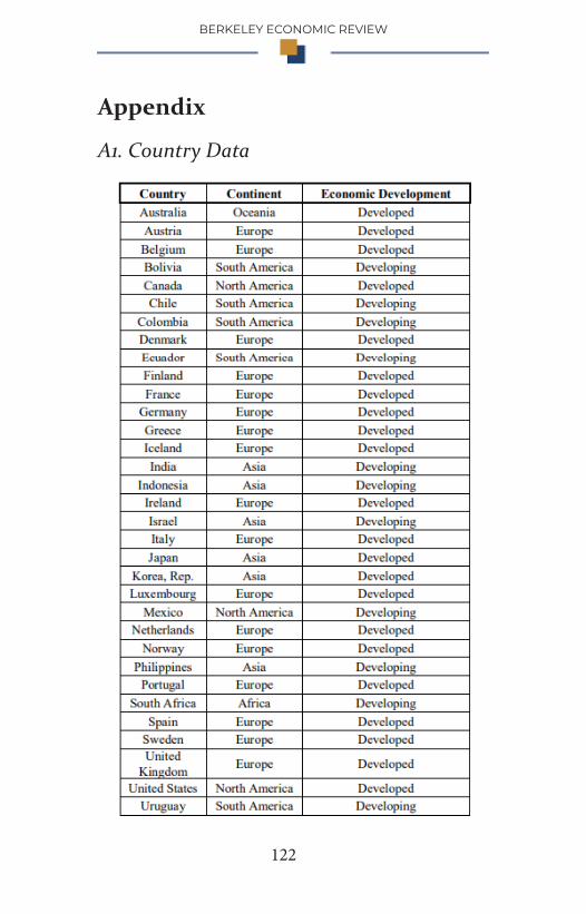
BERKELEY ECONOMIC REVIEW
122
Appendix
A1. Country Data
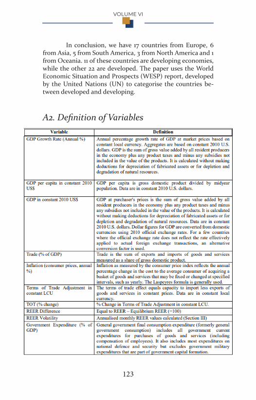
VOLUME VI
123
In conclusion, we have 17 countries from Europe, 6 from Asia, 5 from South America, 3 from North America and 1 from Oceania. 11 of these countries are developing economies, while the other 22 are developed. The paper uses the World Economic Situation and Prospects (WESP) report, developed by the United Nations (UN) to categorise the countries be-tween developed and developing.
A2. Definition of Variables
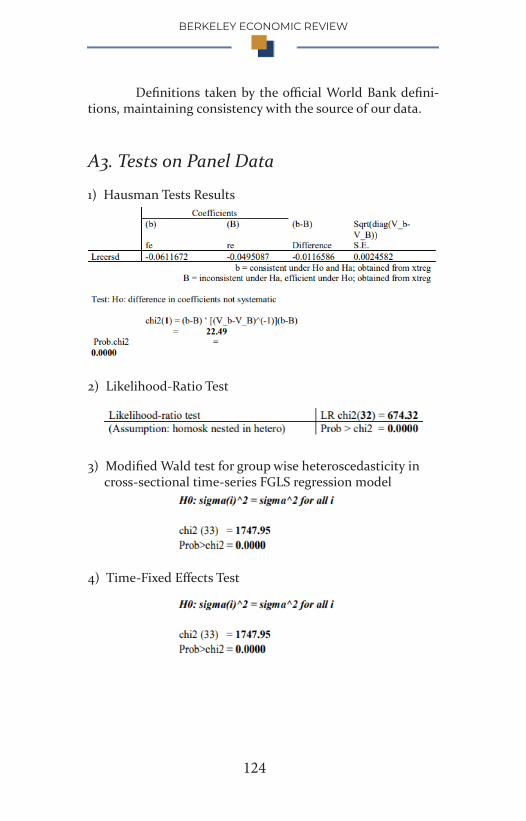
BERKELEY ECONOMIC REVIEW
124
Definitions taken by the official World Bank defini-tions, maintaining consistency with the source of our data.
A3. Tests on Panel Data
1) Hausman Tests Results
2) Likelihood-Ratio Test
3) Modified Wald test for group wise heteroscedasticity in cross-sectional time-series FGLS regression model
4) Time-Fixed Effects Test

VOLUME VI
125
5) Pesaran’s test of cross-sectional dependence and contemporaneous correlation
A4. Correlation between Explanatory Variables
Economic literature suggests that any correlation absolute value below 0.8 is considered sufficiently low to not incur into multicollinearity issues. The table confirms the pa-per’s robustness to this bias.

BERKELEY ECONOMIC REVIEW
126
A5. Diagnostic Testing
Plot of Residuals vs Fitted Values of RegressionNo particular pattern or group of residuals is found.
Plot of Residuals of Main Regression
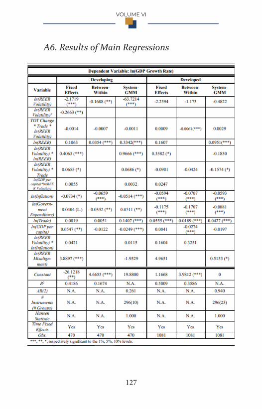
VOLUME VI
127
A6. Results of Main Regressions

BERKELEY ECONOMIC REVIEW
128
Bibliography
Arellano, M., & Bond, S. (191). Some Tests of Specification
for Panel Data: Monte Carlo Evidence and an
Application to Employment equations. Review of
Economic Studies (58), 277-297.
Arellano, M., & Bover, O. (1995). Another Look at the
Instrumental-Variable Estimation of Error-
Components Models. Journal of Econometrics (68),
29-51.
Arize, A., Osang, T., & Slottje, D. (2000). Exchange Rate
Volatility and Foreign Trade: Evidence from Thirtenn
LDCs.Journal of Business and Economics Statistics,
18(1), 10-17.
Bleaney, M., & Greenaway, D. (2001). The Impact of Terms
of Trade and Real Exchange Rate Volatility on
Investment and Growth in Sub-Saharan Africa.
Journal of Development Economics, 65, 491-500.
Blundell, R., & Bond, S. (1998). Initial Conditions and
Moment Restrictions in Dynamic Panel Data
Models. Journal of Econometrics (87), 115-143.
Bollerslev, T. (1986). Generalised Autoregressive Conditional
Heteroscedasticity. Journal of Econometrics (31), 307-
327.
Bruegel (2017). Real effective exchange rates for 178
countries: a new database. Retrieved from Bruegel
[Dataset]: http://bruegel.org/publications/datasets/
real-effective- exchange-rates-for-178-countries-a-
new-database/
Coudert, V., Couharde, C., & Mignon, V. (2008). Do Terms of
VOLUME VI
129
Trade Drive Real Exchange Rates? Comparing Oil
and Commodity Currencies. CEPII.
De Grauwe, P. (1998). Exchange rate variability and the slow
down in growth of international trade. IMF Staff
Papers 35(1), 63-84.
Dollar, D. (1992). Outward Oriented Developing Countries
Really Do Grow More Rapidly. Economic
Development and Cultural Change (4), 523-554.
Driscoll, J., & Kraay, A. (1997). Consistent Covariance Matrix
Estimation with Spatially-Dependent Panel Data.
Review of Economics and Statistics.
Ebaidalla, M. E. (2013). Impact of Exchange Rate Volatility on
Macroeconomic Performance in Sudan. Economic
Research Forum.
Eichengreen, B. (2007). The Real Exchange Rate and
Economic Growth. University of California, Berkeley.
Engle, R. (1982). Autoregressive Conditional
Heteroscedasticity with Estimates of the United
Kingdom Inflation. Econometrica (50), 987-1008.
Franke, G. (1991). Exchange Rate Volatility and International
Trading Strategy. Journal of International Money and
Finance (10), 292-307.
Friedman, M. (1953). The case for flexible exchange rates.
Essays in Positive Economics.
Ghosh, A. R. (1997). Does the Nominal Exchange Rate
Regime Matter? - Working paper 5874. NBER
Working Paper Series.
Ghosh, A., Ostry, J., Gulde, A., & Wolf, H. (1997). Does the
Exchange Rate Regime Matter for Economic Growth?
IMF Economic Issues (2), 1-19.
BERKELEY ECONOMIC REVIEW
130
IMF. (2007). Why Real Exchange Rates. Retrieved from IMF
- Finance and Development: http://www.imf.org/
external/pubs/ft/fandd/2007/09/basics.htm
Jansen, D. (1989). Does Inflation Uncertainty Affect Output
Growth? Further Evidence. The Federal Reserve of
Bank of St.Louis Review, 43-54.
Levy-Yeyati, E., & Edwards, S. (2004). Flexible exchange rates
as shock absorbers. European Economic Review, 1-2.
Levy-Yeyati, E., & Sturzenegger, F. (2002). To Float or to
Fix: Evidence on the Impact of Exchange Rate
Regimes on Growth. American Economic Review.
McKenzie, M. D. (1999). The Impact of Exchange Rate
Volatility on International Trade Flows. Journal of
Economic Surveys (13(1)), 71-106.
Mundell, R. (1973). Uncommon arguments for common
currencies. The Economics of Common Currencies.
Peree, E., & Steinherr, A. (1989). Exchange Rate Uncertainty
and Foreign Trade. European Economic Review (33),
1241-1264.
Pryor, F. (1966). Economic Growth and the Terms of Trade.
Oxford Economics Papers, 18(1), pp. 45-57.
Roodman, D. (2009a). How to do xtabond2: An Introduction
to Difference and System GMM in Stata. Stata
Journal (9), 86-136.
Roodman, D. (2009b). A Note on the Theme of too many
Instruments. Oxford Bulletin of Economics and
Statistics (71), 135-158.
Schnabl, G. (2007). Exchange Rate Volatility and Growth in
Small Open Economies at the EMU Periphery.
Siregar, R., & Rajan , R. (2004). Impact of Exchange Rate

VOLUME VI
131
Volatility on Indonesia's Trade Performance in the
1990s. Journal of the Japanese and International
Economies (18), 218-240.
The World Bank. (2017). World Development Indicators [2017]
[Dataset]. Retrieved from http://data.worldbank.
org/data-catalog/world-development-indicators
United Nations. (2014). Country Classification . Retrieved
from http://www.un.org/en/development/desa/
policy/wesp/wesp_current/2014wesp_countr y_
classification.pdf
Vieira, F. V., Holland, M., Gomes da Silva , C., & Bottecchia,
L. C. (2013). Growth and Exchange Rate Volatility: a
Panel Data Analysis. Applied Economics (45),
3733–3741.
Windmeijer, F. (2005). A Finite Sample Correction for the
Variance of Linear Efficient Two-step GMM
Estimators. Journal of Econometrics, 126(1), 25-51.
Zsolt, D. (2017). Real Effective Exchange Rate for 178
Countries. Bruegel.

BERKELEY ECONOMIC REVIEW
132
Thank you for reading Berkeley Economic Review'sVolume VI
For more content, please visit us at econreview.berkeley.edu