volumetric hilo microscopy employing an electrically ...€¦ · volumetric hilo microscopy...

Volumetric HiLo microscopy employingan electrically tunable lens

Katrin Philipp,1,∗ Andre´ Smolarski,1 Nektarios Koukourakis,1 AndreasFischer,1 Moritz Sturmer,2 Ulrike Wallrabe,2 and Jurgen W Czarske1

1Laboratory for Measuring and Sensor System Techniques, Technische Universitt Dresden,01062 Dresden, Germany

2Laboratory for Microactuators, IMTEK, University of Freiburg, 79110 Freiburg, Germany∗[email protected]

Abstract: Electrically tunable lenses exhibit strong potential forfast motion-free axial scanning in a variety of microscopes. However,they also lead to a degradation of the achievable resolution because ofaberrations and misalignment between illumination and detection opticsthat are induced by the scan itself. Additionally, the typically nonlinearrelation between actuation voltage and axial displacement leads to over- orunder-sampled frame acquisition in most microscopic techniques becauseof their static depth-of-field. To overcome these limitations, we presentan Adaptive-Lens-High-and-Low-frequency (AL-HiLo) microscope thatenables volumetric measurements employing an electrically tunable lens.By using speckle-patterned illumination, we ensure stability against aber-rations of the electrically tunable lens. Its depth-of-field can be adjusteda-posteriori and hence enables to create flexible scans, which compensatesfor irregular axial measurement positions. The adaptive HiLo microscopeprovides an axial scanning range of 1 mm with an axial resolution of about4µm and sub-micron lateral resolution over the full scanning range. Proofof concept measurements at home-built specimens as well as zebrafish em-bryos with reporter gene-driven fluorescence in the thyroid gland are shown.

© 2016 Optical Society of AmericaOCIS codes: (180.2520) Fluorescence microscopy; (180.6900) Three-dimensional mi-croscopy; (220.1080) Active or adaptive optics; (100.6890) Three-dimensional image process-ing.

References and links1. J. Mertz, Introduction to Optical Microscopy (Roberts, 2010).2. M. Minsky, “Memoir on inventing the confocal scanning microscope,” Scanning 10, 128–138 (1988).3. C. Cremer and T. Cremer, “Considerations on a laser-scanning-microscope with high resolution and depth of

field,” Microscopica Acta 81, 31–44 (1974).4. J. Huisken, J. Swoger, F. Del Bene, J. Wittbrodt, and E. H. K. Stelzer, “Optical sectioning deep inside live

embryos by selective plane illumination microscopy,” Science 305, 1007–1009 (2004).5. H.-U. Dodt, U. Leischner, A. Schierloh, N. Jahrling, C. P. Mauch, K. Deininger, J. M. Deussing, M. Eder,

W. Zieglgansberger, and K. Becker, “Ultramicroscopy: three-dimensional visualization of neuronal networksin the whole mouse brain,” Nature Methods 4, 331–336 (2007).

6. M. A. A. Neil, R. Juskaitis, and T. Wilson, “Method of obtaining optical sectioning by using structured light in aconventional microscope,” Opt. Lett. 22, 1905 (1997).

7. P. J. Verveer, Hanley. Q. S., P. W. Verbeek, L. J. Van Vliet, and T. M. Jovin, “Theory of confocal fluorescenceimaging in the programmable array microscope (PAM),” Journal of Microscopy 189, 192–198 (1998).

8. C. Ventalon and J. Mertz, “Quasi-confocal fluorescence sectioning with dynamic speckle illumination,” Opt. Lett.30, 3350 (2005).

#265224 Received 16 May 2016; accepted 20 Jun 2016; published 23 Jun 2016 (C) 2016 OSA 27 Jun 2016 | Vol. 24, No. 13 | DOI:10.1364/OE.24.015029 | OPTICS EXPRESS 15029

9. D. Lim, K. K. Chu, and J. Mertz, “Wide-field fluorescence sectioning with hybrid speckle and uniform-illumination microscopy,” Opt. Lett. 33, 1819–1821 (2008).

10. J. W. Goodman, Speckle Phenomena in Optics: Theory and Applications (Roberts and Company Publishers,2007).

11. J. W. Goodman, “Dependence of image speckle contrast on surface roughness,” Opt. Commun. 14, 324–327(1975).

12. D. Lim, T. N. Ford, K. K. Chu, and J. Mertz, “Optically sectioned in vivo imaging with speckle illuminationHiLo microscopy,” J. Biomed. Opt. 16, 016014 (2011).

13. J. Mertz and J. Kim, “Scanning light-sheet microscopy in the whole mouse brain with HiLo background rejec-tion,” J. Biomed. Opt. 15, 16027 (2010).

14. T. N. Ford, D. Lim, and J. Mertz, “Fast optically sectioned fluorescence HiLo endomicroscopy,” J. Biomed. Opt.17, 21105–21107 (2012).

15. M. A. Lauterbach, E. Ronzitti, J. R. Sternberg, C. Wyart, and V. Emiliani, “Fast Calcium Imaging with OpticalSectioning via HiLo Microscopy,” PloS one 10, e0143681 (2015).

16. N. Koukourakis, M. Finkeldey, M. Sturmer, C. Leithold, N. C. Gerhardt, M. R. Hofmann, U. Wallrabe, J. W.Czarske, and A. Fischer, “Axial scanning in confocal microscopy employing adaptive lenses (CAL),” Opt. Ex-press 22, 6025–6039 (2014).

17. M. Duocastella, G. Vicidomini, and A. Diaspro, “Simultaneous multiplane confocal microscopy using acoustictunable lenses,” Opt. Express 22, 19293–19301 (2014).

18. S. A. Khan and N. A. Riza, “Demonstration of a no-moving-parts axial scanning confocal microscope usingliquid crystal optics,” Opt. Commun. 265, 461–467 (2006).

19. Y. Nakai, M. Ozeki, T. Hiraiwa, R. Tanimoto, A. Funahashi, N. Hiroi, A. Taniguchi, S. Nonaka, V. Boilot,R. Shrestha, J. Clark, N. Tamura, V. M. Draviam, and H. Oku, “High-speed microscopy with an electricallytunable lens to image the dynamics of in vivo molecular complexes,” Rev. Sci. Instrum. 86, 013707 (2015).

20. T. Hinsdale, B. H. Malik, C. Olsovsky, J. A. Jo, and K. C. Maitland, “Volumetric structured illumination mi-croscopy enabled by a tunable-focus lens,” Opt. Lett. 40, 4943–4946 (2015).

21. F. O. Fahrbach, F. F. Voigt, B. Schmid, F. Helmchen, and J. Huisken, “Rapid 3D light-sheet microscopy with atunable lens,” Opt. Express 21, 21010–26 (2013).

22. J. Goodman, Introduction to Fourier Optics (McGraw-Hill, 1996).23. J. Draheim, F. Schneider, T. Burger, R. Kamberger, and U. Wallrabe, in 2010 International Conference on Optical

MEMS and Nanophotonics (OPT MEMS), (2010), pp. 15–16.24. S. J. Kirkpatrick, D. D. Duncan, and E. M. Wells-Gray, “Detrimental effects of speckle-pixel size matching in

laser speckle contrast imaging,” Opt. Lett 33, 2886–2888 (2008).25. M. Imai, “Statistical properties of optical fiber speckles,” Bulletin of the Faculty of Engineering, Hokkaido Uni-

versity 130, 89–104 (1986).26. P. A. Stokseth, “Properties of a Defocused Optical System*,” Journal of the Optical Society of America 59, 1314

(1969).27. D. Kang, E. Clarkson, and T. D. Milster, “Effect of optical aberration on Gaussian laser speckle,” Opt. Express

17, 3084–3100 (2009).28. B. Amos, G. McConnell, and T. WilsonComprehensive Biophysics (Elsevier, 2012).29. R. Opitz, E. Maquet, J. Huisken, F. Antonica, A. Trubiroha, G. Pottier, V. Janssens, and S. Costagliola, “Trans-

genic zebrafish illuminate the dynamics of thyroid morphogenesis and its relationship to cardiovascular develop-ment,” Developmental biology 372, 203–216 (2012).

30. N. C. Shaner, R. E. Campbell, P. A. Steinbach, B. N. G. Giepmans, A. E. Palmer, and R. Y. Tsien, “Improvedmonomeric red, orange and yellow fluorescent proteins derived from Discosoma sp. red fluorescent protein,”Nature Biotech. 22, 1567–1572 (2004).

1. Introduction

Wide field microscopy is well-established in biological and medical applications. At thick sam-ples, however, wide field microscopy suffers from background signals and thus poor contrastand missing depth resolution [1]. In order to provide optical sectioning, many microscopictechniques have been introduced. The most prominent technique is confocal laser scanning mi-croscopy [2, 3], often simply referred to as confocal microscopy. The principle of confocal mi-croscopy is based on the illumination with a diffraction-limited spot and a pinhole-based detec-tion, efficiently eliminating out-of-focus contributions from the sample. Confocal microscopyenables the acquisition of high-contrast, high-resolution data. However, the measurement ratesof confocal microscopy are limited, because scanning is required to perform three-dimensionalmeasurements.


In order to achieve higher measurement rates, alternative techniques rely on illuminating abigger part of the sample and employing a camera for parallel light detection. For instance, lightsheet microscopy is based on only illuminating a thin sheet of the sample and a camera detec-tion [4, 5]. However, light sheet microscopy requires a second optical access and absorption ofthe light sheet becomes a problem for samples with large lateral dimensions. Another camera-based approach is the patterned illumination at the focal plane, which is used in structuredillumination microscopy (SIM) [6] and programmable array microscopy (PAM) [7]. However,these techniques depend heavily on the delivery of a well-defined patterned illumination into thesample. Scattering and aberrations induced by the sample soften the contrast of the patternedillumination and lead to a decreased optical sectioning quality.

Techniques based on speckle illumination like dynamic speckle illumination [8] and High-and-Low-frequency (HiLo) microscopy [9] do not require well-defined nor controlled illumina-tion, because the statistical properties of fully-developed speckles are unaffected by scatteringand aberrations [10, 11]. However, the dynamic speckle illumination microscopy requires sev-eral images in order to reconstruct the high-frequency component of the images. This leadsto a slow data acquisition, if the images are obtained over time or loss in spatial resolution,if the evaluation is conducted in space. The HiLo imaging technique relies on the acquisitionof a second image with uniform illumination to obtain the high-frequency information of theimage. The HiLo technique with speckled illumination was first proposed by Lim et. al [9] andsuccessfully implemented in fluorescence microscopy [12], light sheet microscopy [13] andendomicroscopy [14]. Here, the sample is illuminated by a speckle patterned illumination gen-erated by a laser. The contrast of the speckle illumination is high for the in-focus regions andlow for the out-of-focus regions of the sample. As a consequence, the speckle contrast servesas a weighting function for filtering the out-of-focus contributions of the sample.

While HiLo microscopy provides optically sectioned images with wide field-of-view andhigh speed [15], axial scanning is required for volumetric imaging. Conventionally, this isdone by mechanically moving either the objective or the sample. However, some samples aretoo sensitive to be moved. Moving the objective is slow for heavy objectives due to inertiaand might lead to motion artifacts. Recently, a variety of microscopes such as confocal mi-croscopy [16, 17, 18], wide field microscopy [19], structured illumination microscopy [20] andlight sheet microscopy [21] benefited from using electrically or acoustically tunable lenses foraxial scanning. However, as shown in [16] for confocal microscopy, the axial resolution de-grades with increasing actuation voltages due to increasing aberrations of the tunable lens. Incontrast, HiLo microscopy is expected to be robust against a degradation of the axial resolu-tion due to aberrations, since the speckles that are used for the optical sectioning in the HiLoalgorithm are invariant to aberrations and scattering in the sample (as long as the speckles arefully developed [10, 11]). Another challenge of using tunable lenses for axial scanning is thenonlinear relation between actuation voltage and axial displacement. This leads to irregular ax-ial measurement positions and thus over- or under-sampled frame acquisition. Again, HiLo iscapable of overcoming this limitation because its depth-of-view can be adjusted a-posteriori.

In this paper, we introduce an adaptive lens HiLo (AL-HiLo) microscope that enables volu-metric measurements by employing an electrically tunable lens for axial scanning. We demon-strate that the AL-HiLo compensates for the nonlinear relation between actuation voltage andaxial displacement as well as for the aberrations induced by the tunable lens. The performanceof the setup is characterized and an analysis is given towards the realization of high-throughputscans in zebrafish embryos with reporter gene-driven fluorescence in the thyroid gland. In Sec-tion 2, the theoretical aspects of the HiLo technique are covered. The setup of the AL-HiLomicroscope and characteristics of the electrically tunable lens are described in Section 3. InSection 4, the measurement system is characterized and exemplary measurements are presented


in Section 5. Finally, the results are discussed and an outlook is given in Section 6.

2. HiLo microscopy

HiLo microscopy is based on the acquisition of two images with different type of illumina-tion in order to obtain one optically sectioned image. A uniform-illumination image is usedto obtain the high-frequency (Hi) components of the image, and a nonuniform-illuminationimage is used to obtain the low-frequency (Lo) components of the image. The correspondingintensity distributions of the uniform- and nonuniform-illumination images are denoted as Iu(~r)and In(~r), respectively. The intensity distributions of the high- and low-frequency images arereferred to as ILo(~r) and IHi(~r) with the spatial, two-dimensional coordinates~r. The resultingfull-frequency optically sectioned image is then obtained by

IHiLo(~r) = IHi(~r)+ηILo(~r), (1)

with η being a scaling factor that depends on the experimental configuration of the setup.In order to obtain the high-frequency in-focus components, a typical characteristic of the op-

tical transfer function (OTF) of a standard widefield microscope is exploited: high-frequencycomponents are only well-resolved as long as they are in-focus while low-frequency compo-nents remain visible even if they are out-of-focus [22]. Hence, high-frequency components aredirectly extracted from Iu(~r) using

IHi(~r) = HP{Iu(~r)} , (2)

whereby HP denotes a Gaussian high-pass filter with the cutoff frequency κc applied in thefrequency domain.

The low-frequency component of the image is obtained by calculating

ILo(~r) = LP{CS(~r)Iu(~r)} (3)

with the complimentary low-pass filter LP. The speckle contrast CS(~r) acts as a weightingfunction for extracting the in-focus contributions and rejecting the out-of-focus contributionsof the uniform-illumination image Iu(~r). The overall spatial contrast Cn(~r) is influenced by thespeckles in the illumination as well as sample-induced speckles. In order to correct the influenceof the sample-induced speckles, the difference image

Iδ (~r) = In(~r)− Iu(~r) (4)

is used for speckle contrast calculation. The speckle contrast is defined as

CS(~r) =〈σδ (~r)〉A〈In(~r)〉A

, (5)

where 〈In(~r)〉A and 〈σδ (~r)〉A are the mean of In(~r) and the standard deviation of Iδ (~r), re-spectively. The speckle contrast is calculated over a partition of local evaluation areas A. It isassumed that each area is large enough to encompass several imaged speckle grains. The axialresolution is further increased by applying the band-pass filter

W (~κ) = exp(−|κ

2|2σ2

w

)− exp

(−|κ

2|σ2

w

)(6)

to the difference image Iδ (~r) before evaluating 〈σδ (~r)〉A [9]. As a result, the optical sectioningdepth of the Lo-component can be adjusted by tuning σw. In order to also adjust the optical


sectioning depth of the Hi-component, the cutoff frequency of the Gaussian high pass filter isalso tuned by setting κc = 0.18σw [9].

Since the high- and low-frequency components of the image are now determined, the result-ing optically sectioned HiLo image IHiLo is eventually obtained using (1). As a result, the HiLotechnique provides a powerful method for fast two-dimensional image acquisition, since themeasurement rate equals half of the camera framerate.

3. Experimental setup

In Fig. 1 the experimental setup of the HiLo microscope with an adaptive lens is illustrated. Theillumination is created using a 532 nm laser diode, coupled into a multi mode fiber. The multimode fiber is fixed onto a magnetic metal sheet and can be vibrated by an alternating magneticfield. Consequently, a nonuniform, speckle-patterned as well as a uniform illumination can berealized with a static and vibrating fiber, respectively. The so generated nonuniform or uniformillumination is collimated by the lenses L1 and L2. After passing the beam splitter (BS), thelight enters the illumination arm of the microscope. Here, the light is focused to the sample by alens system consisting of the adaptive lens (AL) with NA≈ 0.05 and refractive power 1/ fAL =−24 . . .25m−1 (see Fig. 2) and the objective lens (OL) with NA = 0.55 and fL = 4.5mm. Theobjective lens is required for achieving a sufficient axial resolution, since the NA of the adaptivelens is too low. The distance between the two lenses amounts to 26mm. Another lens (L3) withf3 = 40mm is then used to image the light onto a CCD camera (pco pixelfly, dynamic range14 Bit and pixel size 6.45µm). A long-pass filter with the cut-on wavelength 550 nm (Thorlabs

BS

AL

OL

L3

camera

specimen

MMF

alternating magnetic field

metal sheet

L1 L2

Fig. 1. Experimental setup. A laser beam is coupled into a multi mode fiber (MMF) that canbe vibrated by alternating magnetic fields. After passing a beam splitter (BS), the light isfocused into the sample by a combination of an adaptive (AL) and an objective lens (OL).The fluorescence light passes the same optical path backwards and is eventually detectedby a camera.

FEL0550) is placed directly in front of the camera for fluorescence measurements.The adaptive lens used for axial scanning is based on the principle described in [23]. The

adaptive lens consists of a transparent Polydimethylsiloxane (PDMS) membrane into whichan annular piezo bending actuator is embedded. An incompressable transparent fluid is filledbetween the membrane and the glass substrate. When actuated, the piezo generates a pressurein the lens which deflects the membrane and thus changes the refractive power. This techniqueenables a large tuning range of the refractive power between 1/ f =−24 . . .25m−1 with appliedvoltages between−40 V and 40 V, see Fig. 2(a). The resonance spectrum of the membrane cen-


ter point deflection in Fig. 2(b) shows that the first resonance mode appears at 250 Hz and hencedriving up to this frequency is possible, although the refractive-power vs. voltage characteristicsis different at resonance mode.

-40 -20 0 20 40

voltage [V]

-40

-20

0

20

40re

frac

tive

pow

er [1

/m]

a) scanning curve

100 101 102 103

frequency [Hz]

0

50

100

150

mea

n de

flect

ion

(rm

s) [µ

m]

b) resonance spectrum

Fig. 2. a) Refractive power of the adaptive lens as a function of the applied voltage withhysteresis behaviour. b) resonance spectrum of a similar electrically tunable lens.

4. Characterization

The relevant properties of the AL-HiLo are discussed in this section. In order to determine theseproperties, a home-built specimen is used. Several rhodamine B-marked micro particles basedon melamine resin are placed onto a glass platelet. The diameter of the micro particles amountsto 10µm with a standard deviation below 0.3µm according to the manufacturer. Since the HiLoalgorithm is based on the evaluation of the speckle-patterns of the non-uniform illumination, inSection 4.1 an overview of the illumination is given.

4.1. Illumination

A small speckle size is desirable, because in HiLo microscopy the axial resolution is inverselyproportional to the speckle frequency and thus scales with speckle size. Additionally, a higheramount of speckles in the evaluation area means higher stability in the speckle contrast de-termination and thus better lateral imaging quality. However, if the smallest speckles size issmaller than 2 px, the speckle contrast is reduced (a speckle size of 1 px leads to a reductionof the speckle contrast by 30 %) [24]. To address these competing requirements, we aimed fora minimal speckle size in the range of 1.5− 2px on the camera, when the sample is in-focus.We employ a multi mode fiber for the generation of the nonuniform illumination, because itproduces fully developed speckles and also provides a high transmission of the laser light. Thecharacteristics of the resulting speckle illumination can be tuned by the numerical aperture NAand the diameter a of the fiber. The minimal speckle size ∆s of the multi mode fiber used in oursetup amounts to ∆s = λ

2·NA = 103nm and the speckle number is N = π(a/∆s)2 = 3 ·108 [25].The measured speckle size on the camera of in-focus images is between 1.5px and 1.6px overthe whole applied actuation voltage range. Taking into account the magnification of the micro-scope (cf. section 4.3), the speckle size on the in-focus plane of the specimen varies between360 nm and 690 nm depending on the actuation voltage of the tunable lens. Since no correlationbetween the speckle size on the camera and the actuation voltage of the tunable lens is observ-able, the size A of the evaluation window for the contrast determination in the HiLo algorithmis held constant for all actuation voltages (A = 7px).


4.2. Axial scanning

In this section the axial displacement of the focus plane is determined as a function of the actu-ation voltage of the tunable lens. For this purpose the home-built specimen with the fluorescentbeads is used as specimen and an axial scan using a motorized stage is conducted for eachactuation voltage. In order to obtain the focus position, the integrated intensity of the resultingHiLo images is determined in dependency of the axial position. As depicted in Fig. 3, a totalscanning range of 1 mm is covered. Note that the tuning range can be adjusted by varying thedistance between adaptive and objective lens. The axial displacement function is nonlinear andshows hysteresis behavior (as expected due to the characteristics of the tunable lens, cf. Fig. 2).As will be shown in the following sections, HiLo microscopy is a suitable tool to cope with

-40 -20 0 20 40

voltage [V]

-800

-600

-400

-200

0

200

400ax

ial d

ispl

acem

ent [

µm] upper arm

lower arm

Fig. 3. Axial scanning curve: Axial displacement as a function of the actuation voltage ofthe electrically tunable lens.

these challenges. In the interests of clarity, the characterizations in the following sections areonly shown for the lower path of the axial scanning curve (cf. red curve in Fig. 3).

4.3. Lateral magnification

The lateral magnification of the AL-HiLo at 0 V actuation voltage of the electrically tunablelens is determined using a 1951 USAF resolution test chart (Thorlabs R1DS1P). Here, thelateral magnification amounts to 20.2. Given a camera resolution of 1392×1040pixels, a totallateral area of 447× 335µm2 can be observed on the specimen. Note that the observable areaas well as the magnification of the system can be adapted to requirements of a given applicationby changing lens L3 and/or changing the distance to the camera.

As the refractive power decreases with increasing actuation voltage (cf. Fig. 2(a)), thelateral magnification is expected to decrease with increased actuation voltage. In order tocharacterize the relative change of the magnification, the home-built specimen consistingof fluorescent beads on a glass plate is used. For every actuation voltage, the specimen ismoved into the focus (cf. Fig 4a). The relative magnification mr is determined as the quo-tient mr(U) = dp(U)/dp(0V), with dp being the distance between two characteristic beads.The resulting relative magnification as a function of the actuation voltage U is illustrated inFig. 4(b). The absolute magnification varies between 27.3 and 13.7. The observable area rangesbetween 334x250µm2 at−40 V and 660x495µm2 at 40 V actuation voltage of the lens. Sincethe speckle size does not scale with the actuation voltage, the parameters of the HiLo algorithmdo not have to be adjusted for each axial position. Consequently, the final HiLo images onlyhave to be re-scaled in order to compensate the voltage-dependent magnification.


a)8fluorescent8particles b)8magnification

408V

-8408V 08V 358V

-40 -20 0 20 40

applied8voltage8[V]

0.6

0.8

1

1.2

rela

tive8

mag

nific

atio

n

Fig. 4. Images of a) fluorescent particles with varying voltage applied at the adaptive lens.The images of the fluorescent particles are a 491x400 pixels-sized subimage taken out ofthe middle of the original camera images. b) The resulting relative magnification normal-ized to the magnification with 0 V actuation voltage.

4.4. Spatial resolution

The upper threshold of the AL-HiLo lateral resolution amounts to

FWHMx,y =0.37λ

NAeff(U)≤ 500nm (7)

with the effective numerical aperture NAeff(U) of the lens system consisting of AL and OL with0.34≤NAeff(U)≤ 0.55 for the full actuation voltage U range. Element 6 of group 7 of the 1951USAF resolution test chart (Thorlabs R1DS1P) is resolved clearly for all voltages applied at theelectrically tunable lens. Consequently, both the theoretical and experimental lateral resolutionshould be well below 2µm.

The axial resolution of the microscope is determined theoretically using the full-width-half-maximum (FWHM) of the point spread function. According Ford et al. [14], the three-dimensional point spread function can be calculated analytically by assuming similar excitationand detection wavelength and applying the Stokseth [26] approximation. As a result, the axialresolution of the low-frequency component equals

FWHMLo ≈0.54

κS ·NAeff(U)(8)

with the speckle frequency κS ≈mr/(2∆S), whereby ∆S denotes the speckle size on the cameraand mr the lateral magnification (cf. Fig. 4). The effective numerical aperture NA is numericallydetermined for the lens system consisting of the adaptive lens (AL) and the objective lens (OL)using the tuning curve of Fig. 2. The FWHM of the high-frequency component is

FWHMHi ≈0.68

κc ·NAeff(U)(9)

with the cutoff frequency κc (cf. Section 2). As shown in Fig. 5(a), the resulting calculated axialresolution for the Hi- and Lo-components is between 3.3µm and 5.4µm and between 900 nmand 2.3µm, respectively, depending on the actuation voltage of the adaptive lens. The decreasedeffective NA with increased absolute value of the actuation voltage of the adaptive lens leadsto a deterioration of the axial resolution with increased actuation voltage. While the resultingaxial resolution of the Hi-component is best at 0 V actuation voltage, the axial resolution of theLo-component enhances with negative actuation voltage of the adaptive lens, because of theincreasing magnification mr and thus increasing speckle frequency κS.

The axial resolution is determined experimentally by using the images obtained in sec-tion 4.2, where an axial scan using a motorized stage was conducted for each actuation voltage.


The FWHM of the corresponding optical sectioning curves determines the axial resolution ofthe AL-HiLo. Assuming Gaussian shaped intensity profiles of the beads as well as a Gaussianshaped point spread function of the microscope, the resulting axial resolution FWHMHiLo,exp isobtained by

FWHMHiLo,exp =√

FWHM2measured−d2

bead (10)

with measured FWHMmeasured of the optical sectioning curve and bead diameter dbead = 10µmaccording to the manufacturer. The errorbars in Fig. 5 indicate the standard deviation of theaxial resolution that is calculated by error propagation of the standard deviation of the parti-cle size. The experimentally and theoretically obtained axial resolutions are generally in goodagreement, whereby the experimentally obtained axial resolutions for the Lo-component seemto face a alight, almost constant shift compared to the theoretical data. This might on the onehand be an effect of the small speckle size of 1.6 px on the camera and consequently a reducedeffective speckle contrast [24]. On the other hand, the speckles in the out-of-focus images mightbe only partially developed, making them sensitive to some aberrations [27]. However, the over-all good fit between experimental and theoretical data suggest, that these effects are small andcan be neglected in most scenarios. As a result, aberrations do not negatively affect the axialresolution within uncertainty limits.

-40 -20 0 20 40

applied voltage [V]

0

2

4

6

8

10

12

axia

l res

olut

ion

[µm

]

a) HiLo

Hi (experiment)

Hi (theory)

Lo (experiment)

Lo (theory)

-40 -20 0 20 40

applied voltage [V]

0

2

4

6

8

10

12ax

ial r

esol

utio

n [µ

m]

b) microscopes

confocal

wide field

HiLo

HiLo (Experiment)

Fig. 5. a) Experimentally and theoretically obtained axial resolution (FWHMs of the pointspread function) for high- and low-frequency components of HiLo images. b) Axial reso-lution of overall HiLo microscopy as well as for confocal and widefield microscopy withidentical objectives.

In order to evaluate the HiLo microscope against state-of-the-art techniques, the axial reso-lution of classical confocal and widefield microscopy are calculated according to [28]

FWHMWideField =0.88λ

n−√

n2−NA2, FWHMConfocal =

0.64λ

n−√

n2−NA2. (11)

Compared to confocal microscopy, HiLo provides similar axial resolution for actuation voltagesof the adaptive lens between−40 V to 20 V and even an enhanced resolution for voltages above20 V, as shown in Fig. 5(b). In conclusion, the axial resolution is about 4µm over the fullscanning range.

4.5. Depth of field adjustment

One of the main benefits of the HiLo technique is the possibility to adjust the depth offield (DOF) a-posteriori by choosing an appropriate depth-of-field multiplier σ−1

w [12]. This


enables flexible scans that compensate the unevenly distributed measurement positions causedby the nonlinear relation between axial displacement and actuation voltage of the electricallytunable lens (cf. Fig. 3(a)). This principle is demonstrated in Fig. 6 using optical sectioningcurves at varying actuation voltages. Analogously as in Section. 4.2 an axial scan is performedover the home-built specimen for each actuation voltage using a motorized stage. The opticalsectioning curves are then determined by integrating the intensity of the obtained HiLo images.As can be seen in Fig. 6, the distance between the peak positions increases with increasingvoltages. Consequently, the depth-of-field (DOF) is also increased with this actuation voltageby tuning the depth-of-field parameter σw in order to compensate for this unevenly distributedaxial measurement positions. As a consequence, the optical sectioning curves intersect at halfof the maximum normalized intensity. That implies a complete covering of the scanned axialposition with optimal use of the obtained frames.

0 50 100 150 200 250 300

axial displacement z [µm]

0

0.2

0.4

0.6

0.8

1

inte

grat

ed in

tens

ity [n

orm

.] -40 V, DOF = 12 µm

-30 V, DOF = 11 µm

-25 V, DOF = 20 µm

-20 V, DOF = 21 µm

-15 V, DOF = 35 µm

-10 V, DOF = 52 µm

50 % baseline

Fig. 6. a) Optical sectioning curves of HiLo images for six selected actuation voltages.Adjusting the depth-of-fields (DOF) of the HiLo mechanism ensures that the full axialrange is covered. Simultaneously the optical sections are as thin as possible.

In conclusion, the HiLo technique is able to compensate the main drawbacks of axial scan-ning using an electrically tunable lens, namely deteriorating axial resolution caused by aber-rations and unevenly distributed axial measurement positions caused by the nonlinear axialdisplacement function (cf. Fig. 3). Furthermore, volumetric HiLo microscopy profits from themain advantages of axial scanning. On the one hand HiLo is able to exhaust the potential forhigh speed measurements, because HiLo provides a full frame by only acquiring two imagesand thus is in principle capable for measurement times of the half of the camera exposure andacquisition time. On the other hand, adaptive HiLo microscopy does not rely on any mechani-cal scanning, because axial scanning is conducted using the electrically tunable lens and lateralscanning is not required because of the wide field of view enabled by the HiLo technique.

5. Measurements

In this section volumetric measurements are conducted by tuning the actuation voltage of thelens. A compensation for the voltage-dependent magnification is conducted by re-scaling theimages after the HiLo algorithm is executed. Since the speckle size does not change with vary-ing voltage, no adaption of the HiLo technique is necessary.

Two different operation modi of the axial scan using the tunable lens are possible:

(a) one scanning cycle with uniform- and a second cycle with nonuniform-illumination


(b) alternating images with uniform and nonuniform illumination directly after each other.

Modus (a) has the advantage, that the scanning process is faster than for modus (b), be-cause there is less time needed for switching the illumination source. In contrast, modus (b)is more robust against the hysteresis behavior of the electrically tunable lens as well as cross-sensitivities between refractive power of the lens and ambient atmospheric pressure and tem-perature. Since at this stage speed is not in the scope of this paper, we use the second modus inour setup.

The following measurements are conducted with a actuation voltage step width of 40 mV.

5.1. Demonstration measurement

In order to demonstrate the optical sectioning and axial scanning capability of the adaptiveHiLo microscope, a specimen consisting of several fluorescent beads with a diameter of about10µm separated by a thin foil is investigated. In Fig. 7(a-c) the uniformly illuminated imagesare shown for different axial scanning depths, whereby HiLo images for different scanningdepths are shown in 7(d-f). While the marked beads are visible in all images obtained by usingthe uniform illumination, the out-of-focus contributions are rejected in the HiLo images.

a) uniform, z = 20 µm

bead #1bead #2

b) uniform, z = 34 µm

bead #1bead #2

c) uniform, z = 40.5 µm

bead #1bead #2

d) HiLo, z = 20 µm

bead #1bead #2

e) HiLo, z = 34 µm

bead #1bead #2

f) HiLo, z = 40.5 µm

bead #1bead #2

Fig. 7. a-c) Selected images with uniform illumination. d-f) Selected HiLo images for dif-ferent axial planes. The axial scanning is conducted by tuning the adaptive lens.

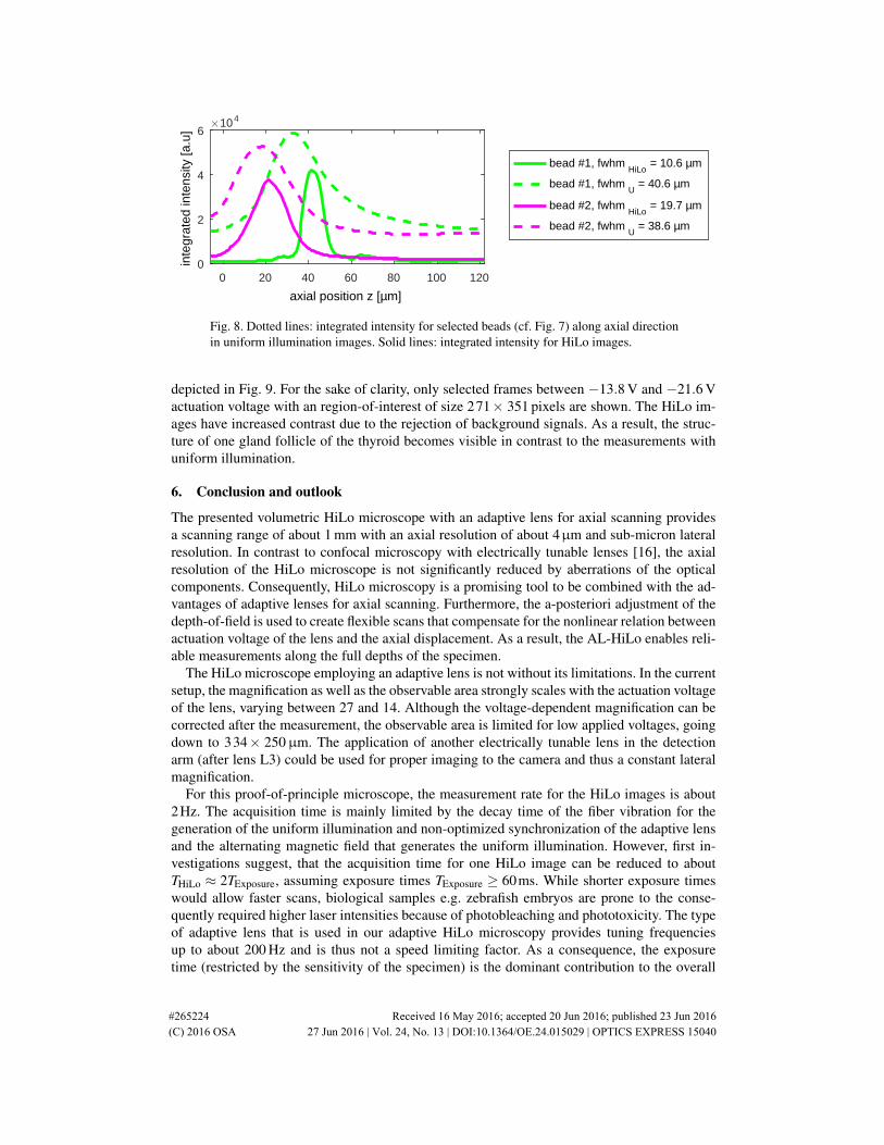
For a clearer illustration of the optical sectioning capability, the integrated intensity in themarked region-of-interests is integrated along z-direction. As depicted in Fig. 8, the HiLo algo-rithm enables optical sectioning in contrast to the standard widefield technique.

5.2. Zebrafish measurements

The microscope is used for investigating reporter gene-driven fluorescence in the thyroid glandof zebrafish embryos. Zebrafish embryos are used as experimental model in basic and appliedresearch since the large number of produced embryos, their size and optical transparency pro-vide various experimental advantages and screening opportunities. Furthermore, the princi-pal similarity of vertebrates allow to derive information relevant for understanding of humandiseases. Particularly their high transmission rate makes them an ideal candidate for opticalmeasurements. Transgenic zebrafish embryos have been used to understand the dynamics ofthyroid morphogenesis [29]. Here, the thyroid is marked with the mCherry protein[30]. Themaximum excitation wavelength is 587 nm. With a quantum yield of 0.22, this amounts to afluorescence yield of 8.36 % at the used laser wavelength of 532 nm. The maximum emissionwavelength is 610 nm. The resulting fluorescence HiLo images of a thyroid gland follicle are


0 20 40 60 80 100 120

axial position z [µm]

0

2

4

6

inte

grat

ed in

tens

ity [a

.u]

×104

bead #1, fwhmHiLo

= 10.6 µm

bead #1, fwhmU

= 40.6 µm

bead #2, fwhmHiLo

= 19.7 µm

bead #2, fwhmU

= 38.6 µm

Fig. 8. Dotted lines: integrated intensity for selected beads (cf. Fig. 7) along axial directionin uniform illumination images. Solid lines: integrated intensity for HiLo images.

depicted in Fig. 9. For the sake of clarity, only selected frames between −13.8 V and −21.6 Vactuation voltage with an region-of-interest of size 271× 351 pixels are shown. The HiLo im-ages have increased contrast due to the rejection of background signals. As a result, the struc-ture of one gland follicle of the thyroid becomes visible in contrast to the measurements withuniform illumination.

6. Conclusion and outlook

The presented volumetric HiLo microscope with an adaptive lens for axial scanning providesa scanning range of about 1 mm with an axial resolution of about 4µm and sub-micron lateralresolution. In contrast to confocal microscopy with electrically tunable lenses [16], the axialresolution of the HiLo microscope is not significantly reduced by aberrations of the opticalcomponents. Consequently, HiLo microscopy is a promising tool to be combined with the ad-vantages of adaptive lenses for axial scanning. Furthermore, the a-posteriori adjustment of thedepth-of-field is used to create flexible scans that compensate for the nonlinear relation betweenactuation voltage of the lens and the axial displacement. As a result, the AL-HiLo enables reli-able measurements along the full depths of the specimen.

The HiLo microscope employing an adaptive lens is not without its limitations. In the currentsetup, the magnification as well as the observable area strongly scales with the actuation voltageof the lens, varying between 27 and 14. Although the voltage-dependent magnification can becorrected after the measurement, the observable area is limited for low applied voltages, goingdown to 334× 250µm. The application of another electrically tunable lens in the detectionarm (after lens L3) could be used for proper imaging to the camera and thus a constant lateralmagnification.

For this proof-of-principle microscope, the measurement rate for the HiLo images is about2Hz. The acquisition time is mainly limited by the decay time of the fiber vibration for thegeneration of the uniform illumination and non-optimized synchronization of the adaptive lensand the alternating magnetic field that generates the uniform illumination. However, first in-vestigations suggest, that the acquisition time for one HiLo image can be reduced to aboutTHiLo ≈ 2TExposure, assuming exposure times TExposure ≥ 60ms. While shorter exposure timeswould allow faster scans, biological samples e.g. zebrafish embryos are prone to the conse-quently required higher laser intensities because of photobleaching and phototoxicity. The typeof adaptive lens that is used in our adaptive HiLo microscopy provides tuning frequenciesup to about 200 Hz and is thus not a speed limiting factor. As a consequence, the exposuretime (restricted by the sensitivity of the specimen) is the dominant contribution to the overall


a) HiLo images

b) uniform illumination

Fig. 9. a) HiLo images and b) images with uniform illumination of reporter-gene drivenmcherry fluorescence of transgenic zebrafish. The fluorescence is regulated by part of thepromotor region of the thyreoglobulin gene, coding for a thyroid hormone precursor. Theoptical sectioning provided by the HiLo algorithm leads to the rejection of the out-of-focus contributions and thus increased contrast of the images compared to the uniformlyilluminated images. Scalebar is 10µm.

measurement time of the full specimen. As a result, the prospective time for a full volumetriccharacterization should be approximately 2NTExposure with N being the number of frames peraxial scan.

As a demonstration of the optical sectioning capability of the AL-HiLo microscope, a home-built specimen and a transgenic zebrafish embryo was investigated. In contrast to wide fieldmicroscopy, the contrast of the HiLo images was increased due to the rejection of out-of-focussignals. The huge field-of-view of the HiLo microscope and the high axial scanning range of thetunable lens enables three-dimensional measurements over a huge volume. The potentially highscanning frequency of the tunable lens up to 250 Hz and no need for lateral scanning makes theAL-HiLo a promising candidate for high-throughput characterization of zebrafish embryos suchas functional genetics to study organ differentiation or responses to drug/chemical exposure.

Acknowledgments

The financial support of the Deutsche Forschungsgemeinschaft (DFG) for the project CZ 55/32-1 and Wa1657-6 is gratefully acknowledged. The authors also thank Hannes Radner for pro-viding the controlling of the adaptive lens. We thank Stefan Scholz of Helmholtz Centre forEnvironmental Research GmbH for providing the samples and fruitful discussions.


volumetric hilo microscopy employing an electrically ...€¦ · volumetric hilo microscopy...

Documents