VOLUMETRIC SCANNING FOR EXTERNAL CORROSION MEASUREMENT

Sergio Néstor Río 1

, Pablo Federico Cosentino 1

1. TGS Argentina

INTRODUCTION

Old pipelines are sensitive to external corrosion; this defect can generally be found in both,

longitudinal and axial position along the spool. Picture 1 shows the defect that we usually find in the

field; identifying each defect’s shape, its depth and interaction with other defects turns out to be a

craft task.

In old pipelines such measurement is a complicated job. Generally the corrosion defect is located at

the bottom of the pipeline and evaluation engineers have to work in bad weather conditions.

TGS has pointed out that this task should be automated, in order to achieve this goal TGS has

made an research and develop interdisciplinary agreement with scientists from Balseiro Institute,

near Bariloche City in Argentina, where Nuclear Engineers and Physicists obtain their degrees.

Besides, scientists have teamed up with TGS engineers to do this project.

After analyzing different alternatives to measure the defects, the laser optical sensor technique was

selected.

APPROACH

The process of detection and identification of external corrosion in pipelines can be synthesized in

the following stages:

� Run High Resolution Smart pigs inspections (ILI) to identify corroded areas in the pipeline.

� Digging affected zones: the zones identified during the previous procedure are exposed for their direct examination

� Visual examination of corrosion affected zones: These zones are divided in grids for their analysis.

� Manual shape and depth corrosion measurements

� Damage assessment according to international standards

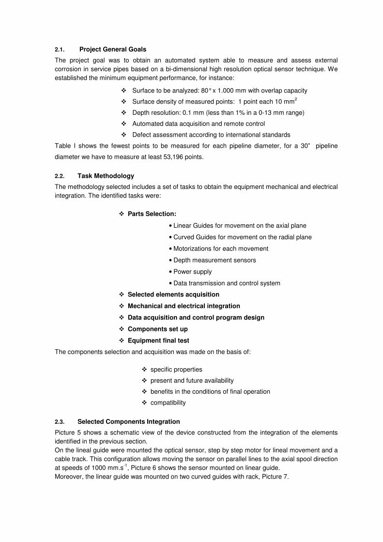
The hardest task is the corrosion depth measurement, we normally use depth gauges, Picture 2

shows this kind of gauges, the maximum defect depth at defined intervals will be measured to

obtain the worst profile, but in old pipelines such measurement is a complicated job, generally the

corrosion defect is located at the bottom of the pipeline and evaluation engineers have to work in

bad weather conditions, Picture 3.

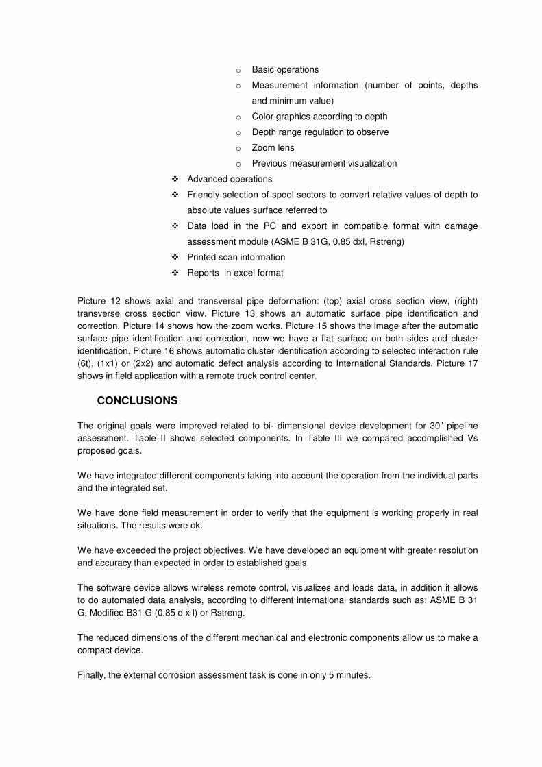
Picture 4 shows a scheme of a pipeline wall thickness, the red painted zone is the corrosion defect.

Our goal is to determine, as accurately as we can, the corrosion area dimensions in order to obtain

the Pipeline Failure Stress.

2.1. Project General Goals

The project goal was to obtain an automated system able to measure and assess external

corrosion in service pipes based on a bi-dimensional high resolution optical sensor technique. We

established the minimum equipment performance, for instance:

� Surface to be analyzed: 80° x 1.000 mm with overlap capacity

� Surface density of measured points: 1 point each 10 mm2

� Depth resolution: 0.1 mm (less than 1% in a 0-13 mm range)

� Automated data acquisition and remote control

� Defect assessment according to international standards

Table I shows the fewest points to be measured for each pipeline diameter, for a 30” pipeline

diameter we have to measure at least 53,196 points.

2.2. Task Methodology

The methodology selected includes a set of tasks to obtain the equipment mechanical and electrical

integration. The identified tasks were:

� Parts Selection:

• Linear Guides for movement on the axial plane

• Curved Guides for movement on the radial plane

• Motorizations for each movement

• Depth measurement sensors

• Power supply

• Data transmission and control system

� Selected elements acquisition

� Mechanical and electrical integration

� Data acquisition and control program design

� Components set up

� Equipment final test

The components selection and acquisition was made on the basis of:

� specific properties

� present and future availability

� benefits in the conditions of final operation

� compatibility

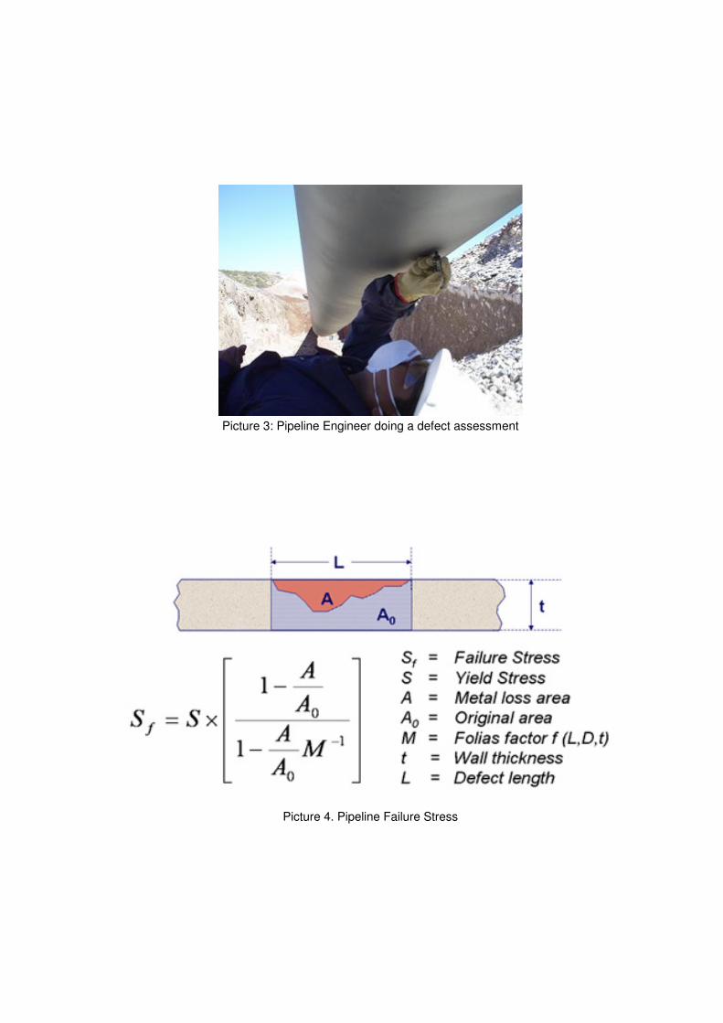
2.3. Selected Components Integration

Picture 5 shows a schematic view of the device constructed from the integration of the elements

identified in the previous section.

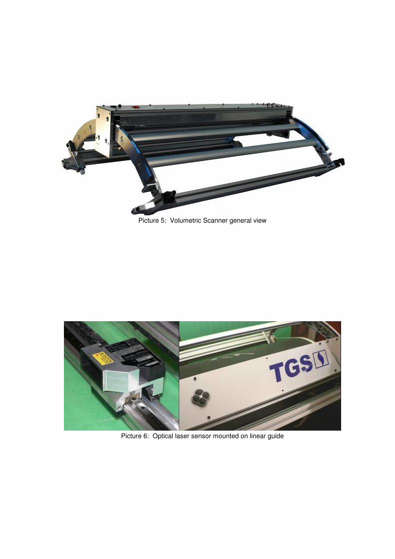
On the lineal guide were mounted the optical sensor, step by step motor for lineal movement and a

cable track. This configuration allows moving the sensor on parallel lines to the axial spool direction

at speeds of 1000 mm.s-1

, Picture 6 shows the sensor mounted on linear guide.

Moreover, the linear guide was mounted on two curved guides with rack, Picture 7.

The combination of a motor step by step, a gear and a series of bearings especially adapted to the

curved guides, allows moving the linear guide following the spool curvature, Picture 8.

Above linear guide and fix in it a box is located that contains electrical and electronic system

components included Bluetooth antenna, Picture 9.

The advance system, programmed by a controller located in the mentioned box, acts so that the

sensor scans a line in axial sense and the following line in the opposite axial sense, reducing the

data acquisition time.

The data acquired by the sensor is stored in the controller and it is transmitted periodically to the

control PC, Picture 10.

The subjection system to the spool is realized using tape and tensors, Picture 11.

2.4. Measurement and Control Parameters

According to previous experience during the tests stage control, data acquisition and user

interaction were separated.

To do the sensor automatic and controlled movement and its data acquisition feasible, a

programmable controller is used (PLC).

Based on parameters defined for the equipment and of a unique order issued from the commander

computer, the sensor carriage can do automatically the following movements:

� Movement in the axial sense (1000 mm) with:

o Constant speed during the measurement length

o Desacceleration ramp at the end of the route

� Advance in the cross-sectional sense to the axis (approximately 3 mm

on the surface of the spool)

� Carriage return according to the sequence before indicated, including

acceleration ramp generation with constant speed and desacceleration

ramp in this process

� Depth measurements readings during the axial movement, obtaining 1

point each 0.95 mm approximately

� Data transmission from the equipment to command computer on regular

intervals.

2.5. Software and Hardware

Our own development program called “Pit Explorer” allows us to visualize and keep the obtained

data, Picture 12.

The developed control software enables the user to be in touch with the equipment, enter and load

parameters from the measurement, conduct measurement operations (start and shutdown), locking

and data record at regular intervals (each 5 lines of measurement).

The program was made in last generation compliable visual language, feasible within the

surroundings of Microsoft Windows (98, 2000, XP).

Software characteristics:

� Run in a standard personal computer (PC)

� Visual surroundings of clear and unequivocal interpretation of the

parameters meaning and emergent orders

� Laser sensor connection by Bluetooth system

� Images handling, including:

o Basic operations

o Measurement information (number of points, depths

and minimum value)

o Color graphics according to depth

o Depth range regulation to observe

o Zoom lens

o Previous measurement visualization

� Advanced operations

� Friendly selection of spool sectors to convert relative values of depth to

absolute values surface referred to

� Data load in the PC and export in compatible format with damage

assessment module (ASME B 31G, 0.85 dxl, Rstreng)

� Printed scan information

� Reports in excel format

Picture 12 shows axial and transversal pipe deformation: (top) axial cross section view, (right)

transverse cross section view. Picture 13 shows an automatic surface pipe identification and

correction. Picture 14 shows how the zoom works. Picture 15 shows the image after the automatic

surface pipe identification and correction, now we have a flat surface on both sides and cluster

identification. Picture 16 shows automatic cluster identification according to selected interaction rule

(6t), (1x1) or (2x2) and automatic defect analysis according to International Standards. Picture 17

shows in field application with a remote truck control center.

CONCLUSIONS

The original goals were improved related to bi- dimensional device development for 30” pipeline

assessment. Table II shows selected components. In Table III we compared accomplished Vs

proposed goals.

We have integrated different components taking into account the operation from the individual parts

and the integrated set.

We have done field measurement in order to verify that the equipment is working properly in real

situations. The results were ok.

We have exceeded the project objectives. We have developed an equipment with greater resolution

and accuracy than expected in order to established goals.

The software device allows wireless remote control, visualizes and loads data, in addition it allows

to do automated data analysis, according to different international standards such as: ASME B 31

G, Modified B31 G (0.85 d x l) or Rstreng.

The reduced dimensions of the different mechanical and electronic components allow us to make a

compact device.

Finally, the external corrosion assessment task is done in only 5 minutes.

REFERENCES

• Argentine Standard for Natural Gas Transport and Distribution Networks (NAG 100).

• ASME B 31 G Manual for Determining the Remaining Strength of Corroded Pipelines.

• Pipeline Research Council International (PRCI) Report 3-805 a Modified Criterion for

Remaining Strength of Corroded Pipelines.

LIST TABLES

Table I Points to be measured for each pipeline diameter

Table II Selected components

Component Proprieties

Structural frame Build with aluminum structural profile

Linear movement: frame Transmission: By rack for land use.

Length: 1200 mm. Standard Carriage.

Maximum speed: 1500 mm.s-1

. Final run

sensors.

Linear movement : motor Working principle: step by step,

longitudinal resolution half step: 0,09 mm,

weight: 400 g.

Radial movement: frame Stainless Steel, 90° sections with rack.

Final run sensors.

Radial movement : motor Step by step motor. With reduction gear.

Weight: 1.3 kg.

Depth sensor

Working principle: laser triangulation,

span: 25 mm, resolution: 1 µm, sampling

rate: up to 1200 samples.s-1

Global control

Programmable PLC.

Feature Goal Result

Analysis area 80° x 1000 mm 80° x 1000 mm

Points to be

measured

53.196 points 1 point 0,95 mm axial

section

1 axial line each 3 mm

cross section

185.964 points in the

area

Measurements

density 1 point each 10 mm

2

3.5 point each 10 mm2

Depth resolution 0.1 mm Resolution: 0.02 mm

Accuracy: 0.1 – 0.2 mm

Scanning time 20 minutes 5 minutes

Table III. Final goals, task accomplished

LIST OF FIGURES

Picture 1: General External Corrosion Defect

Picture 2: Manual Corrosion Dimension Measurement

Picture 3: Pipeline Engineer doing a defect assessment

Picture 4. Pipeline Failure Stress

Picture 5: Volumetric Scanner general view

Picture 6: Optical laser sensor mounted on linear guide

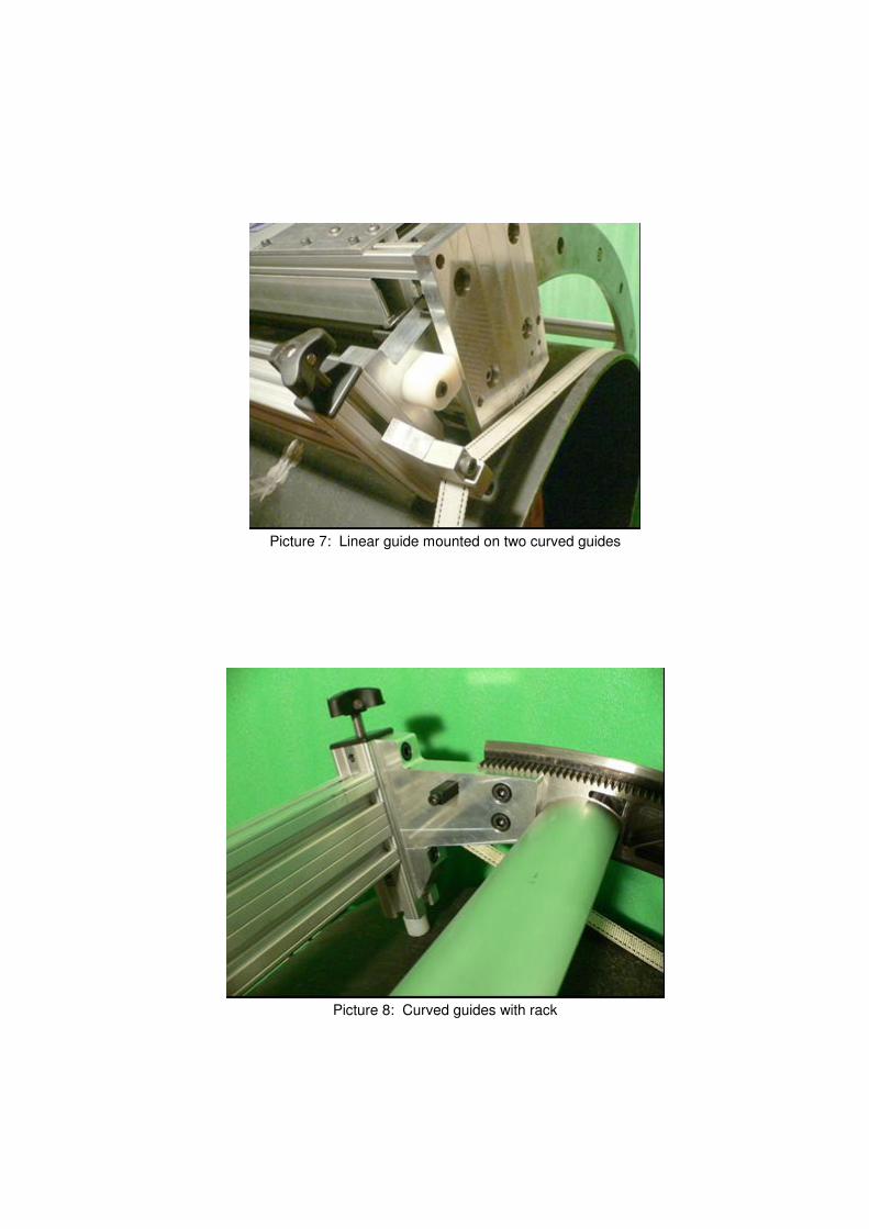
Picture 7: Linear guide mounted on two curved guides

Picture 8: Curved guides with rack

Picture9: Bluetooth system mounted on upper box

Picture10: Controller located in the upper box

Picture 11: Subjection system to the spool is realized using tape and tensors

Picture 12: Corrosion view by “ Pit Explorer” software as measured

x, y, z defect

position

Corrosion defect

Cursor

Features Tree

Corrosion profile

Tape and Tensor

Support System

Pipe deformation

Picture 13: Axial and transversal pipe deformation (Top) axial cross section view

(Left) transverse cross section view

Picture 14: Here we can see how the zoom works

Automatic clean surface pipe

identification and correction

Corrosion Defect Zoom

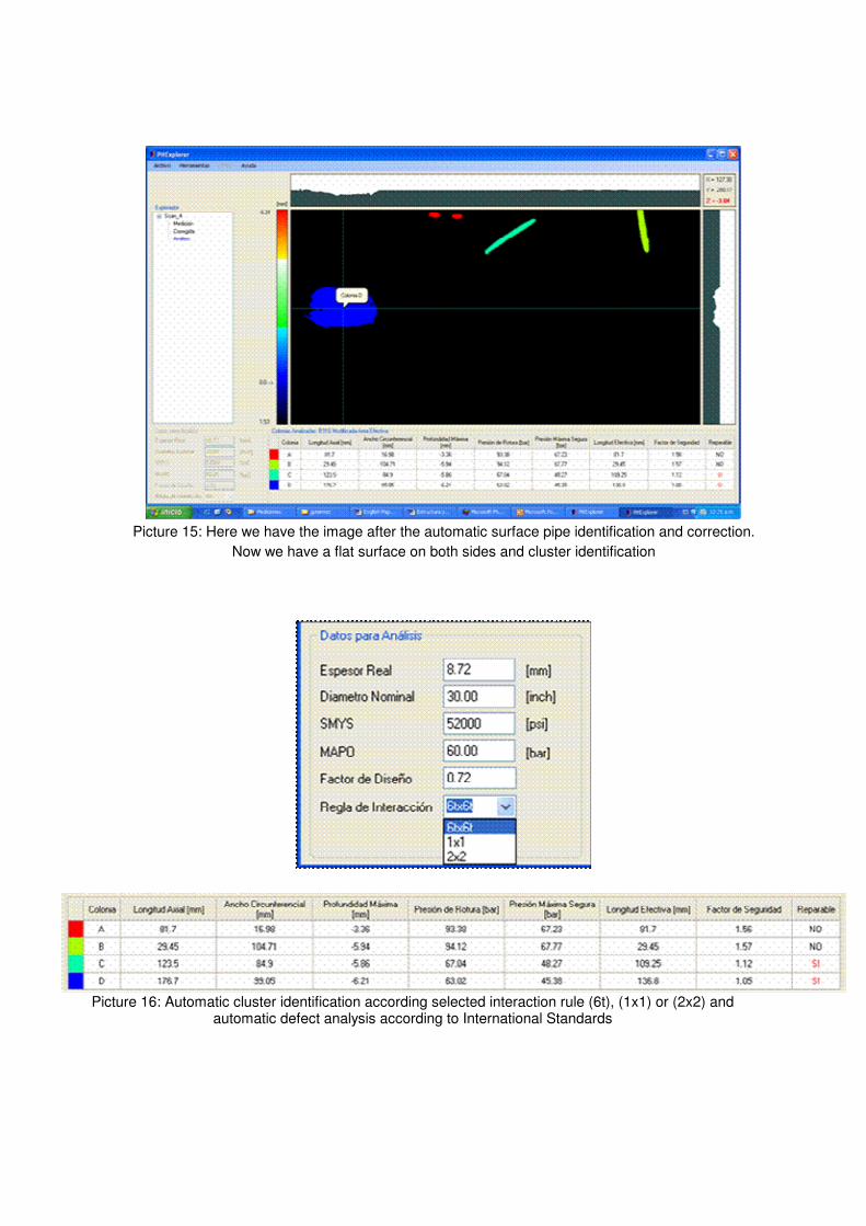
Picture 15: Here we have the image after the automatic surface pipe identification and correction.

Now we have a flat surface on both sides and cluster identification

Picture 16: Automatic cluster identification according selected interaction rule (6t), (1x1) or (2x2) and automatic defect analysis according to International Standards

Picture 17: View of equipment installed in 30” pipeline with a truck control center