vortex induced fatigue damage of a steel catenary riser near
TRANSCRIPT

Vortex Induced Fatigue Damage of a Steel Catenary Riser near the Touchdown Point
Emir Lejlic
Marine Technology
Supervisor: Carl Martin Larsen, IMTCo-supervisor: Per Erlend Voie, DNV
Department of Marine Technology
Submission date: June 2013
Norwegian University of Science and Technology


NTNU Trondheim
Norwegian University of Science and Technology
Faculty of Engineering Science and Technology
Department of MarineTechnology
1
M.Sc. thesis 2013 for
Stud.tech. Emir Lejlic
VORTEX INDUCED FATIGUE DAMAGE OF STEEL CATENARY
RISERS NEAR THE TOUCHDOWN POINT.
Slender flexible structures in a marine environment like steel catenary risers (SCR) will expe-
rience conditions with insignificant wave forces in combination with strong current. In such
cases the structural response will be dominated by vortex-induced vibrations (VIV). Although
amplitudes are small compared to wave induced stresses, fatigue damage can be high because
of the large number of stress cycles that may occur. State-of-the-art VIV fatigue design pro-
grams such as VIVANA, make the best use of available knowledge, but remain limited for
several reasons in their capacity to capture the broad complexity of the phenomenon. In addi-
tion to more generic uncertainties with regard to structural capacity, like variations in material
properties or S-N curves, much uncertainty is linked to the amount and relevance of data
available to understand VIV itself. Time domain computation of VIV have been attempted,
however most empirical models for VIV prediction are based on frequency domain analysis
which imply certain limitations as to how geometry, boundary conditions and loads can be
modelled.
A key issue in design of SCRs is to control stresses and fatigue damage in the touch down
area. Dynamic bending stresses will vary along the SCR but a large peak will almost always
be seen near the touch down point. This peak is caused by the restrictions on riser displace-
ments from the presence of the seafloor, and the local bending stresses will be influenced by
stiffness and damping properties of the bottom. Analysis models based on finite elements will
represent the interaction between riser and seafloor by discrete springs, which in linear fre-
quency domain analysis will remain constant independent of the displacements. This type of
model may give a significant over-prediction of bending stresses at the touch down point since
a linear spring will give tensile forces instead of being released and allowing the pipe to lift
off from the bottom. Actually the touch down point moves with time, due to platform motions
mainly, leading to more evenly distributed fatigue damage.
The objective of the master thesis will be to:
1. Find relevant literature about VIV and SCRs and give an overview of the topics.
2. Learn to use relevant software, such as SIMA, RIFLEX, VIVANA and BATCH-
scripting.
3. Identify key variables and perform a fatigue sensitivity analysis with the VIVANA soft-
ware.
4. Use data given from DNV and create a probability distribution of mean floater position
to be used for calculation of fatigue from VIV.
5. Describe and investigate a method for distributing accumulated fatigue damage in the
touch down area based on considerations of platform motions statistics.

NTNU Faculty of Marine Technology
Norwegian University of Science and Technology Department of Marine Structures
2
The work may show to be more extensive than anticipated. Some topics may therefore be left
out after discussion with the supervisor without any negative influence on the grading.
The candidate should in her/his report give a personal contribution to the solution of the prob-
lem formulated in this text. All assumptions and conclusions must be supported by mathe-
matical models and/or references to physical effects in a logical manner. The candidate should
apply all available sources to find relevant literature and information on the actual problem.
The report should be well organised and give a clear presentation of the work and all conclu-
sions. It is important that the text is well written and that tables and figures are used to sup-
port the verbal presentation. The report should be complete, but still as short as possible.
The final report must contain this text, an acknowledgement, summary, main body, conclu-
sions and suggestions for further work, symbol list, references and appendices. All figures,
tables and equations must be identified by numbers. References should be given by author
name and year in the text, and presented alphabetically by name in the reference list. The re-
port must be submitted in two copies unless otherwise has been agreed with the supervisor.
The supervisor may require that the candidate should give a written plan that describes the
progress of the work after having received this text. The plan may contain a table of content
for the report and also assumed use of computer resources. From the report it should be possi-
ble to identify the work carried out by the candidate and what has been found in the available
literature. It is important to give references to the original source for theories and experi-
mental results. The report must be signed by the candidate, include this text, appear as a pa-
perback, and - if needed - have a separate enclosure (binder, DVD/ CD) with additional mate-
rial.
The work will be carried out in cooperation with Det Norske Veritas, Trondheim
Contact person at DNV is Per Erlend Voie.
Supervisor at NTNU is Professor Carl M. Larsen.
Carl M. Larsen
Submitted: January 2013
Deadline: 10 June 2013

Abstract
In this thesis, the fatigue damage of a steel catenary riser was investigated, especially in thevicinity of the touchdown point.
The steel catenary riser is a promising riser solution due to its simplicity and low cost.This is in particular true if the motions in heave direction are modest. As the offshoreindustry is moving into deeper waters, riser solutions will need to be designed with highsafety, to ensure interests both economically and environmentally. Understanding how thestructure reacts to forces from the environment is therefore of great concern. It is experiencedthat the steel catenary riser will have a noticeable increase in the fatigue damage in theproximity of the touchdown zone. This is the area where the riser has contact with thesea bottom. The sea bottom will impose forces on the riser, and because of the increasedcurvature of the structure in this area, the stresses will be magnified. This pipe–soil interac-tion seems to be highly non-linear and it is complex to model the riser realistically in this area.
When an ocean current passes the riser, it may form vortices that are shed from both sidesof the pipe. If these vortices are shed with a frequency near the natural frequency of theriser, the pipe may start to vibrate. This response is called vortex induced vibration, andthe phenomenon is important in riser design. Even if the amplitudes are small compared tovessel induced motions, the high number of cycles may give a significant contribution to thetotal fatigue damage.
In this work, the fatigue damage initiated by the vortex induced vibrations has been inves-tigated, and fatigue analyses of a steel catenary riser have been carried out. In order toperform such analysis taking into account vortex induced vibrations, the computer programVIVANA has been used. VIVANA is an empirical computer program based on experimentsand computes the vortex induced response in the frequency domain. In the frequency domain,the pipe–sea floor interaction is modelled with discrete springs at the nodes where the risertouches the ground. However, these springs are not released if the riser is lifted, somethingwhich gives non-realistic stresses in the area.
An alternative way of analysing the fatigue damage near the touchdown area has beenproposed and performed. The analysis was based on floater motion statistics, and simulationswere done changing the floater offset. The final fatigue result was found by summation ofindividual fatigue results for different coordinates of the floater in the XY-plane. The resultsindicated that the fatigue damage was evenly distributed in the proximity of the touchdownarea, and the maximum and overall damage were reduced.
iii


Sammendrag
Denne masteroppgaven har fokusert på utmattingsskade av et stigerørkonsept (Steel CatenaryRiser) i nærheten av havbunnen.
Stigerøret har en buet form og er en lovende stigerørsløsning grunnet dens enkelthet oglave kostnad. Dette er spesielt sant dersom den vertikale fartøysbevegelsen er moderat. Daoffshore-næringen beveger seg mot stadig dypere farvann vil det kreves nye stigerørsløsninger,som er designet med høy sikkerhet, for å sikre økonomiske og miljømessige interesser. Å forståhvordan konstruksjonen reagerer på miljøkrefter er derfor av stor interesse. Det er observertat stigerøret vil ha en betydelig økning i utmattingsskaden i nærheten av landingssonen.Dette er området hvor stigerøret møter sjøbunnen. Sjøbunnen vil påføre krefter på stigerøretog grunnet den høye kurvaturen i området, vil man merke en økning i trykkspenningene.Denne interaksjonen hvor røret møter havbunnen er av ikke-lineær natur, og modelleringenav stigerøret er vanskelig og må gjøres i tidsdomenet.
Når en havstrøm driver forbi stigerøret, kan det oppstå virvler som blir avløst på hverside av konstruksjonen. Dersom virvlene blir avløst med en frekvens som er i nærhetenav egenfrekvensen til stigerøret, kan det begynne å vibrere. Denne responsen er kalt forvirvelindusert vibrasjon, og har stor betydning for potensielle utmattingsskader. Selv omresponsamplitudene er små i forhold til fartøyinduserte bevegelser, kan det høye antalletsykluser gi et signifikant bidrag til utmattingsskaden.
I denne oppgaven har utmattingsskaden grunnet virvelavløsninger blitt undersøkt. For åutføre slike analyser har dataprogrammet VIVANA blitt brukt. VIVANA er et empiriskdataprogram og er basert på eksperimenter. Det beregner virvelindusert respons i frekvens-domenet. I frekvensdomenet er rør-havbunn interaksjonen modellert med diskrete fjær vednodene som er i kontakt med havbunnen. Problemet er at disse fjærene ikke vil slippestigerørsmodellen dersom den er løftet fra bakken. Dette skaper dermed falske krefter somgir konservative resultater i dette området.
En alternativ analysemetode av utmattingsskaden i landingssonen har blitt foreslått ogundersøkt i oppgaven. Analysen baserte seg på statistikk av fartøysbevegelse, og simuleringerble gjort i VIVANA. Den endelige utmattingsskaden ble funnet ved summering av deindividuelle utmattingsskadene ved forskjellige posisjoner av fartøysbevegelsen. Resultatetindikerte at skaden ble jevnere fordelt i nærheten av landingssonen, og den samlede ogmaksimale skaden på stigerøret ble redusert.
v


Acknowledgement
This work was carried out at the Department of Marine Technology, at the NorwegianUniversity of Science and Technology (NTNU), in cooperation with Det Norske Veritas(DNV) under the supervision of Professor Carl Martin Larsen, and under co-supervision ofengineer Per Erlend Voie from DNV in Trondheim. I would like to thank them both for theassistance I have received during the semester. Professor Carl Martin Larsen has helped methroughout the semester with weekly meetings and conversations. This has been greatly ap-preciated. I am thankful to Per Erlend Voie for his scripting knowledge which has been helpful.
Thanks to my friends at the office and school for five good years here at the university. Thediscussions with the guys from the office have been of great importance. I also want to thankmy family for all their support during my study years.
Lastly, I would like to thank my beautiful Idunn for always believing in me.
Emir Lejlic,Trondheim, Monday 10th June, 2013
vii


Notation
AbbreviationsCF Cross flow
FE Finite Element
FPSO Floating Production, Storage and Offloading
IL In line
JONSWAP Joint North Sea Wave Project
RAO Response Amplitude Operator
RHoP Riser hang off point
RP Recommended practice
SCF Stress concentration factor
SCR Steel Catenary Riser
St Strouhal number
TDP Touchdown point
TDZ Touch down zone
TLP Tension leg plattform
VIM Vortex induced motion
VIV Vortex induced vibrations
Greek Symbolsα Proportionality factor
ε Phase angle
ν Kinematic viscosity.
ωn Natural frequency n
ix

ξ Structural damping ratio
Roman symbolsfi Non-dimensional frequency
C Damping matrix
K Stiffness matrix
M Mass matrix
r,r,r Displacement, velocity and acceleration vectors.
X Excitation force vector
A/D Amplitude ratio
Ast Cross section steel area
D Diameter of structure
E Elastic modulus
Ei/n Excitation parameter for frequency i or n
f0 Eigenfrequency in still water
fv Vortex shedding frequency
Fe,CF CF excitation force
fosc Oscillating frequency
Hs Significant wave height
I Second moment of area.
k Spring stiffness
l Length of riser
m Mass per length
ma0 Added mass
n Mode number
T Top tension
Tp Peak period
x

tref Reference thickness
U Current velocity
Ur Reduced velocity
Wy/z Section modulus for bending about y- and z-axis
Re Reynold number
xi


Contents
Abstract iii
Sammendrag v
Acknowledgement vii
Notation xi
1 Introduction 11.1 Steel Catenary Risers . . . . . . . . . . . . . . . . . . . . . . . . . . . . . . . 21.2 Pipe – sea floor iteration. . . . . . . . . . . . . . . . . . . . . . . . . . . . . . 21.3 Time or frequency domain analysis . . . . . . . . . . . . . . . . . . . . . . . 31.4 Non-stationary VIV of slender beams . . . . . . . . . . . . . . . . . . . . . . 41.5 Ocean current . . . . . . . . . . . . . . . . . . . . . . . . . . . . . . . . . . . 4
1.5.1 High velocity current in the North Sea . . . . . . . . . . . . . . . . . 51.5.2 Current variability . . . . . . . . . . . . . . . . . . . . . . . . . . . . 6
2 VIV 72.1 Introduction . . . . . . . . . . . . . . . . . . . . . . . . . . . . . . . . . . . . 72.2 Important remarks . . . . . . . . . . . . . . . . . . . . . . . . . . . . . . . . 82.3 Eigenfrequency . . . . . . . . . . . . . . . . . . . . . . . . . . . . . . . . . . 102.4 Excitation force . . . . . . . . . . . . . . . . . . . . . . . . . . . . . . . . . . 112.5 Free oscillation test . . . . . . . . . . . . . . . . . . . . . . . . . . . . . . . . 112.6 Forced oscillation test . . . . . . . . . . . . . . . . . . . . . . . . . . . . . . . 132.7 Added mass . . . . . . . . . . . . . . . . . . . . . . . . . . . . . . . . . . . . 142.8 Suppression of VIV . . . . . . . . . . . . . . . . . . . . . . . . . . . . . . . . 152.9 Time and space sharing . . . . . . . . . . . . . . . . . . . . . . . . . . . . . 15
3 Soil Interaction 193.1 Introduction . . . . . . . . . . . . . . . . . . . . . . . . . . . . . . . . . . . . 193.2 Pipe–soil response . . . . . . . . . . . . . . . . . . . . . . . . . . . . . . . . . 203.3 Dynamic interaction of catenary risers with the sea floor . . . . . . . . . . . 22
4 Fatigue 234.1 Introduction . . . . . . . . . . . . . . . . . . . . . . . . . . . . . . . . . . . . 234.2 SCR fatigue design . . . . . . . . . . . . . . . . . . . . . . . . . . . . . . . . 234.3 Selection of SN curve . . . . . . . . . . . . . . . . . . . . . . . . . . . . . . . 24
xiii

4.4 Effect of floater type on SCR fatigue . . . . . . . . . . . . . . . . . . . . . . 264.5 Fatigue Reliability Analysis . . . . . . . . . . . . . . . . . . . . . . . . . . . 264.6 Fatigue Analysis in VIVANA . . . . . . . . . . . . . . . . . . . . . . . . . . . 29
4.6.1 Introduction . . . . . . . . . . . . . . . . . . . . . . . . . . . . . . . . 294.6.2 Generation of time series . . . . . . . . . . . . . . . . . . . . . . . . . 30
5 Software 335.1 SIMA and RIFLEX . . . . . . . . . . . . . . . . . . . . . . . . . . . . . . . . 335.2 SIMO . . . . . . . . . . . . . . . . . . . . . . . . . . . . . . . . . . . . . . . 335.3 VIVANA . . . . . . . . . . . . . . . . . . . . . . . . . . . . . . . . . . . . . . 335.4 Analysis with RIFLEX and VIVANA . . . . . . . . . . . . . . . . . . . . . . 34
5.4.1 Analysis Procedure . . . . . . . . . . . . . . . . . . . . . . . . . . . . 345.5 BATCH-scripting . . . . . . . . . . . . . . . . . . . . . . . . . . . . . . . . . 375.6 MATLAB . . . . . . . . . . . . . . . . . . . . . . . . . . . . . . . . . . . . . 38
5.6.1 Flow chart for processing the vessel motion data . . . . . . . . . . . . 40
6 Riser configuration 41
7 Parameter variation analysis 437.1 Introduction . . . . . . . . . . . . . . . . . . . . . . . . . . . . . . . . . . . . 437.2 Current profile and direction . . . . . . . . . . . . . . . . . . . . . . . . . . . 437.3 Bottom properties . . . . . . . . . . . . . . . . . . . . . . . . . . . . . . . . . 447.4 Relative damping . . . . . . . . . . . . . . . . . . . . . . . . . . . . . . . . . 457.5 Number of elements . . . . . . . . . . . . . . . . . . . . . . . . . . . . . . . . 457.6 S-N curve selection . . . . . . . . . . . . . . . . . . . . . . . . . . . . . . . . 467.7 Info about the results . . . . . . . . . . . . . . . . . . . . . . . . . . . . . . . 467.8 Results . . . . . . . . . . . . . . . . . . . . . . . . . . . . . . . . . . . . . . . 47
7.8.1 Run 1-4 . . . . . . . . . . . . . . . . . . . . . . . . . . . . . . . . . . 477.8.2 Run 5-7 . . . . . . . . . . . . . . . . . . . . . . . . . . . . . . . . . . 497.8.3 Run 8-11 . . . . . . . . . . . . . . . . . . . . . . . . . . . . . . . . . . 517.8.4 Run 12-14 . . . . . . . . . . . . . . . . . . . . . . . . . . . . . . . . . 537.8.5 Run 15-18 . . . . . . . . . . . . . . . . . . . . . . . . . . . . . . . . . 557.8.6 Run 19-22 . . . . . . . . . . . . . . . . . . . . . . . . . . . . . . . . . 57
8 Variation of vessel offset analysis. 598.1 Introduction . . . . . . . . . . . . . . . . . . . . . . . . . . . . . . . . . . . . 598.2 Analysis steps . . . . . . . . . . . . . . . . . . . . . . . . . . . . . . . . . . . 608.3 Vessel motion . . . . . . . . . . . . . . . . . . . . . . . . . . . . . . . . . . . 61
8.3.1 Raw data from SIMO analysis . . . . . . . . . . . . . . . . . . . . . . 618.4 Transforming the coordinates . . . . . . . . . . . . . . . . . . . . . . . . . . 62
8.4.1 Vessel motion probability . . . . . . . . . . . . . . . . . . . . . . . . . 638.5 Summary of the counting procedure . . . . . . . . . . . . . . . . . . . . . . . 638.6 Reducing the motion information . . . . . . . . . . . . . . . . . . . . . . . . 65
8.6.1 Discrete coordinates . . . . . . . . . . . . . . . . . . . . . . . . . . . 668.7 Calculation steps. . . . . . . . . . . . . . . . . . . . . . . . . . . . . . . . . . 71
xiv

8.8 Current profile probability . . . . . . . . . . . . . . . . . . . . . . . . . . . . 738.9 Effective tension . . . . . . . . . . . . . . . . . . . . . . . . . . . . . . . . . . 74
8.9.1 Effects on fatigue damage . . . . . . . . . . . . . . . . . . . . . . . . 748.10 Sector discretisation issues . . . . . . . . . . . . . . . . . . . . . . . . . . . . 75
8.10.1 Probability variation . . . . . . . . . . . . . . . . . . . . . . . . . . . 778.11 Results . . . . . . . . . . . . . . . . . . . . . . . . . . . . . . . . . . . . . . . 81
9 Conclusions 859.1 Parametric study . . . . . . . . . . . . . . . . . . . . . . . . . . . . . . . . . 859.2 Variation of vessel position . . . . . . . . . . . . . . . . . . . . . . . . . . . . 86
10 Discussion 87
11 Recommendation for further work 89
Bibliography 92
Appendices I
A Data files IA.1 Input files . . . . . . . . . . . . . . . . . . . . . . . . . . . . . . . . . . . . . IA.2 Variation text files . . . . . . . . . . . . . . . . . . . . . . . . . . . . . . . . I
A.2.1 variations.txt file for the parameter variation study . . . . . . . . . . IA.3 Files from the SIMO analysis . . . . . . . . . . . . . . . . . . . . . . . . . . IIIA.4 BATCH-scripts . . . . . . . . . . . . . . . . . . . . . . . . . . . . . . . . . . III
A.4.1 BATCH-script used for parameter variation study. . . . . . . . . . . . IIIA.4.2 BATCH-script used for variation of vessel coordinate analysis . . . . V
A.5 Matlab files . . . . . . . . . . . . . . . . . . . . . . . . . . . . . . . . . . . . VIIA.5.1 Run file for processing of the motion file from SIMO, process_x_y_pos.mVIIA.5.2 read_xy_data.m . . . . . . . . . . . . . . . . . . . . . . . . . . . . . XIA.5.3 find_extreme_coord.m . . . . . . . . . . . . . . . . . . . . . . . . . . XIIIA.5.4 transform_xy_data.m . . . . . . . . . . . . . . . . . . . . . . . . . . XIVA.5.5 count_in_large_matrix.m . . . . . . . . . . . . . . . . . . . . . . . . XIVA.5.6 xy_count_and_prob.m . . . . . . . . . . . . . . . . . . . . . . . . . XVIA.5.7 convert_xy_to_polar_xy.m . . . . . . . . . . . . . . . . . . . . . . .XVIIA.5.8 search_xy_in_sectors.m . . . . . . . . . . . . . . . . . . . . . . . . .XVIIIA.5.9 Run file for summing the fatigue damages at different coordinates,
run_variation.m . . . . . . . . . . . . . . . . . . . . . . . . . . . . .XXIVA.5.10 save_run_xy_info_in_struct.m . . . . . . . . . . . . . . . . . . . . .XXVIIIA.5.11 add_fatigue_damage_to_struct.m . . . . . . . . . . . . . . . . . . . XXXA.5.12 sum_fatigue_damage_from_xy_variation.m . . . . . . . . . . . . . XXXA.5.13 find_important_parameters_resfile.m . . . . . . . . . . . . . . . . .XXXI
xv

List of Figures
1.1 Example of three riser types. . . . . . . . . . . . . . . . . . . . . . . . . . . . 11.2 Pipe – sea floor interaction model. . . . . . . . . . . . . . . . . . . . . . . . . 31.3 Steel catenary riser plane. . . . . . . . . . . . . . . . . . . . . . . . . . . . . 41.4 Definition of current direction. . . . . . . . . . . . . . . . . . . . . . . . . . . 41.5 Top tensioned riser and steel catenary riser. . . . . . . . . . . . . . . . . . . 5
2.1 Vortex shedding. . . . . . . . . . . . . . . . . . . . . . . . . . . . . . . . . . 72.2 CF and IL motion. . . . . . . . . . . . . . . . . . . . . . . . . . . . . . . . . 72.3 Amplitude ratio for a specific reduced velocity. . . . . . . . . . . . . . . . . . 82.4 Strouhal numbers in VIVANA . . . . . . . . . . . . . . . . . . . . . . . . . . 92.5 Response amplitude versus Ur. Courtesy of Larsen (2011). . . . . . . . . . . 92.6 Example of three modes. . . . . . . . . . . . . . . . . . . . . . . . . . . . . . 102.7 Empirical lift coefficient curve. . . . . . . . . . . . . . . . . . . . . . . . . . . 112.8 Examples of CF + IL trajectory. . . . . . . . . . . . . . . . . . . . . . . . . . 132.9 Contour plot of CF coefficient. Courtesy of Larsen (2011) . . . . . . . . . . . 142.10 Riser with helical strakes. . . . . . . . . . . . . . . . . . . . . . . . . . . . . 152.11 Excitation zones for space sharing frequencies. . . . . . . . . . . . . . . . . . 162.12 Time sharing process. . . . . . . . . . . . . . . . . . . . . . . . . . . . . . . . 162.13 Excitation zones for time sharing frequencies. . . . . . . . . . . . . . . . . . 17
3.1 Touchdown zone interaction. . . . . . . . . . . . . . . . . . . . . . . . . . . . 193.2 Penetration curve for determination of linear spring stiffness. . . . . . . . . . 213.3 Free body diagram of riser model and soil. . . . . . . . . . . . . . . . . . . . 21
4.1 Example of SN curve . . . . . . . . . . . . . . . . . . . . . . . . . . . . . . . 254.2 Examples of offshore drilling types. . . . . . . . . . . . . . . . . . . . . . . . 26
5.1 RIFLEX–VIVANA flow chart. . . . . . . . . . . . . . . . . . . . . . . . . . . 345.2 Response frequencies. . . . . . . . . . . . . . . . . . . . . . . . . . . . . . . . 355.3 Flow chart of a BATCH-process. . . . . . . . . . . . . . . . . . . . . . . . . 385.4 Flow chart of Matlab functions used in the variation of vessel coordinate analysis. 40
6.1 Riser configuration example, ZX-plane. . . . . . . . . . . . . . . . . . . . . . 416.2 Riser configuration example, XY-plane. . . . . . . . . . . . . . . . . . . . . . 41
7.1 Riser segments . . . . . . . . . . . . . . . . . . . . . . . . . . . . . . . . . . 467.2 Results from parameter run 1-4. . . . . . . . . . . . . . . . . . . . . . . . . . 477.3 Response amplitudes of Run 4. . . . . . . . . . . . . . . . . . . . . . . . . . 48
xvi

7.4 Excitation zones of Run 4. . . . . . . . . . . . . . . . . . . . . . . . . . . . . 487.5 Results from parameter run 5-7. . . . . . . . . . . . . . . . . . . . . . . . . . 497.6 Results from parameter run 8-11. . . . . . . . . . . . . . . . . . . . . . . . . 517.7 Results from parameter run 12-14. . . . . . . . . . . . . . . . . . . . . . . . . 537.8 Results from parameter run 15-18. . . . . . . . . . . . . . . . . . . . . . . . . 557.9 Results from parameter run 19-22. . . . . . . . . . . . . . . . . . . . . . . . . 57
8.1 Example of changing TDP. . . . . . . . . . . . . . . . . . . . . . . . . . . . . 598.2 Example of vessel motion. . . . . . . . . . . . . . . . . . . . . . . . . . . . . 618.3 Vessel motion of 0-360◦ . . . . . . . . . . . . . . . . . . . . . . . . . . . . . . 628.4 Vessel motion of 0◦ . . . . . . . . . . . . . . . . . . . . . . . . . . . . . . . . 628.5 Original and transformed coordinate system. . . . . . . . . . . . . . . . . . . 628.6 Scatter representation of the vessel motion. . . . . . . . . . . . . . . . . . . . 658.7 Scatter representation of the vessel motion. Close to the origin . . . . . . . . 658.8 Probability of motion coordinates. . . . . . . . . . . . . . . . . . . . . . . . . 668.9 Sector with three part. . . . . . . . . . . . . . . . . . . . . . . . . . . . . . . 678.10 Sector with two parts . . . . . . . . . . . . . . . . . . . . . . . . . . . . . . . 678.11 Example of four sectors of 90◦ each that cover all the vessel motion points.
Each sector consists of three sector parts. . . . . . . . . . . . . . . . . . . . . 678.12 Largest radius of a vessel motion point. . . . . . . . . . . . . . . . . . . . . . 688.13 Discrete (x, y) points. . . . . . . . . . . . . . . . . . . . . . . . . . . . . . . . 698.14 The probability of the discrete coordinates. . . . . . . . . . . . . . . . . . . . 698.15 Surface plot. . . . . . . . . . . . . . . . . . . . . . . . . . . . . . . . . . . . . 708.16 Contour plot. . . . . . . . . . . . . . . . . . . . . . . . . . . . . . . . . . . . 708.17 Discrete points used in analysis. . . . . . . . . . . . . . . . . . . . . . . . . . 718.18 Example of fatigue damage on riser. . . . . . . . . . . . . . . . . . . . . . . . 738.19 Effective tension of the lower riser part. . . . . . . . . . . . . . . . . . . . . . 758.20 The effective tension at the RHoP for all the runs. . . . . . . . . . . . . . . . 758.21 Difference of sector parts. . . . . . . . . . . . . . . . . . . . . . . . . . . . . 768.22 x-coordinate of maximum probability. . . . . . . . . . . . . . . . . . . . . . . 788.23 y-coordinate of maximum probability. . . . . . . . . . . . . . . . . . . . . . . 788.24 Maximum probability convergence. . . . . . . . . . . . . . . . . . . . . . . . 788.25 Maximum probability convergence (closer). . . . . . . . . . . . . . . . . . . . 788.26 Alterations of the probability contour. . . . . . . . . . . . . . . . . . . . . . 808.27 Normalized fatigue. Variation analyis vs. original. . . . . . . . . . . . . . . . 818.28 Closer look at TDP. . . . . . . . . . . . . . . . . . . . . . . . . . . . . . . . . 818.29 Contour of the effective tension when RHoP is at (xi, yi) . . . . . . . . . . . 82
xvii

List of Tables
4.1 Parameters for the sensitivity study. . . . . . . . . . . . . . . . . . . . . . . . 274.2 Riser data in parameter study . . . . . . . . . . . . . . . . . . . . . . . . . . 284.3 Results from the sensetivity study. . . . . . . . . . . . . . . . . . . . . . . . 294.4 VIVANA methods for fatigue calculation . . . . . . . . . . . . . . . . . . . . 29
6.1 Data of the SCR. . . . . . . . . . . . . . . . . . . . . . . . . . . . . . . . . . 41
7.1 Current profiles. . . . . . . . . . . . . . . . . . . . . . . . . . . . . . . . . . . 447.2 Current directions used in parameter study. . . . . . . . . . . . . . . . . . . 507.3 Bottom stiffness values used in the parameter analysis. . . . . . . . . . . . . 527.4 Values of relative damping used in the parameter study. . . . . . . . . . . . . 547.5 Number of elements used in the parameter study. . . . . . . . . . . . . . . . 567.6 S-N curves used in the parameter study. . . . . . . . . . . . . . . . . . . . . 58
8.1 Example of (x, y) motion file. . . . . . . . . . . . . . . . . . . . . . . . . . . 618.2 Example of transformed data. . . . . . . . . . . . . . . . . . . . . . . . . . . 648.3 variations.txt file for the coordinate variation. . . . . . . . . . . . . . . . . 728.4 Example of a fatigue.txt file. . . . . . . . . . . . . . . . . . . . . . . . . . . . 738.5 Add caption . . . . . . . . . . . . . . . . . . . . . . . . . . . . . . . . . . . . 758.6 Probability at the discrete points. . . . . . . . . . . . . . . . . . . . . . . . . 768.7 Number of sectors, maximum probability and its coordinates. . . . . . . . . . 798.8 Probability of x-position of the vessel. . . . . . . . . . . . . . . . . . . . . . . 838.9 Probabilty of tension at RHoP. . . . . . . . . . . . . . . . . . . . . . . . . . 83
xviii

Chapter 1Introduction
The offshore industry is moving towards deeper waters, and floating facilities have thereforebecome an integral part of many field developments that are working as an oil and gasproduction facility, and as a hubs for developments of several remote wells or fields. The steelcatenary riser (SCR) has become a good option for oil and gas export from these floatingfacilities to shallow water platforms, or to subsea hubs. The advantage of the SCR is its lowcost compared to other riser designs such as flexible pipes that have complex set of layers,and which do not have the same resistance to hydrostatic pressure as rigid steel pipes. Theuse of SCRs within the industry has created a need of understanding their behaviour duringinstallation, operation and nevertheless, under extreme conditions [1].
In the touchdown zone (TDZ), where the riser meets the sea bottom, the catenary shape ofthe riser will impose high stresses to the riser structure. This will be of particular importancedue to the motions of the floating structure with varying degrees of freedom. The vesselmotion causes the riser to move in different directions, and the touchdown zone will thereforevary in time. The dynamics of the floater and the ocean current will have a great effect onthe riser. The restraints that the sea floor causes will give large fatigue damage in this area.One uses finite element (FE) models to represent the interaction between the sea floor andthe riser. However, modelling the interaction is a difficult task with many uncertainties. Theinteraction model may be represented by discrete springs.
Top tensioned riser. Steel catenary riser. Lazy
wave
riser.
Buoyancy modules.Touchdown
point.
Figure 1.1: Example of three riser types.
In this work it has been investigated how vortex induced vibrations (VIV) influence the
1

1.1. STEEL CATENARY RISERS
fatigue damage near the sea floor. VIV is a resonance phenomenon that is caused by vorticesthat are shed from both sides of the riser structure as the ocean current drifts past the pipe.In the offshore industry it is common to consider the ocean current coming from one direction,either parallel to the riser plane or orthogonal. Today, risers are being used in extreme depths,where the ocean current velocity may vary along the depth. It is therefore challenging to es-timate an exact damage the riser will accumulate by VIV that is initiated by the ocean current.
In order to calculate VIV problems, several computer programs have been created. They aremostly based on empirical models on the assumption that VIV will appear as a response atone or a limited number of discrete frequencies. These computer programs are constantlychanging as researches get new experimental results. In the work done during this masterthesis, the computer programme VIVANA has been used to investigate how fatigue damageis accumulated near the touchdown zone of a steel catenary riser.
1.1 Steel Catenary RisersFloating production systems must rely on some kind of marine risers for transport of thewell-stream from the sea floor to the platform. In many cases they also need risers to transportprocessed oil and gas down to a pipeline. Among many different riser concepts, the steelcatenary riser is promising due to its simplicity and low cost. This is in particular true if theheave motions of the floater are moderate, which is the case for tension leg platforms (TLP),SPAR buoys and deep drought floaters.
A key issue in the design of catenary risers is to control the stresses and the fatigue damage inthe touchdown zone. Vessel motions and waves will cause time varying stresses and because ofthe boundary conditions such stresses will often have the largest values in this area. Anotherimportant phenomenon that may contribute significantly to the fatigue is the VIV causedby the ocean current. Although the stress amplitudes are smaller compared to wave motioninduced stresses, fatigue damage may be high due to the high number of cycles that may occur.
A catenary riser is different from a tensioned riser in the sense that the current will have a flowdirection relative to the pipe axis different from 90◦. The basis for almost all empirical VIVmodels are experiments with oncoming flow perpendicular to the cylinder [2]. A consequenseof this is that there are many uncertainties related to the hydrodynamics of catenary risers.Some of these uncertainties are the Strouhal number (St), added mass (MA)and the liftcoefficients. Comparing tests and analyses is therefore of great interest.
1.2 Pipe – sea floor iteration.It is well known that the fatigue process is controlled by local stress variations at the pointwhere the crack growth takes place. It is also known that maximum bending stress in catenaryrisers will in most cases occur close to the touchdown point (TDP), and that the stressgradient is large in the vicinity of this point. Another fact is that vessel motions and riser
2

CHAPTER 1. INTRODUCTION
dynamics will cause the TDP to move, and thus move the stress profile along the riser.Fatigue analyses must therefore consider true movement of the TDP as well as dynamic stressvariations.
Spring
Dashpot
Node
Riser touching
the sea floor.
Figure 1.2: Pipe – sea floor interaction model.
If a finite element method is usedfor stress analysis, one may modelthe pipe – sea floor interaction byintroducing non-linear springs anddashpots at nodes with bottom con-tact. This is illustrated in Figure1.2. Both the springs and dashpotsare only active when there is seafloor contact at the node. Thismeans that the nodes may lift offrom the sea floor without experi-encing extra tensile forces from thesprings and dashpots. On the otherhand, if the riser is pressed downwards against the seabed, the springs and dashpots will getactive and prevent penetration of the sea floor by compression forces.
This type of model will require a fully non-linear dynamic analysis in time domain. Suchanalyses are demanding with regard to computer resources and are therefore often replaced bylinear approaches, which is used in this work. In linear approaches the springs and dashpotswill not let go of the pipe if it is lifted from the sea floor, creating unrealistic tensile forces inthe TDP area.
1.3 Time or frequency domain analysisEmpirical models used for VIV analysis are today almost exclusively based on the assumptionthat VIV will appear as a response at discrete frequencies. The benefit of applying a frequencydomain method is that needed coefficients are found from fixed frequency experiments andhence directly applicable. A time domain approach needs in principle transient hydrodynamiccoefficients or a strategy for frequency identification. This makes the hydrodynamic modelcomplicated, but the advantage is that this model can be combined with a non-linear finiteelement code and thereby take into account the non-linear pipe – sea floor interaction. In[3] the authors describe how a new approach using both a linear frequency domain modelfor VIV calculations and a non-linear model for time domain analysis is used. The firststeps were to carry out the VIV analysis according to linear theory and then introduce thecalculated hydrodynamic forces to a non-linear structural model. The results showed that
• The combined use of frequency and time domain were well suited for investigating theinfluence from local non-linearities on stresses from VIV.
• The TDP represented a non-linear boundary condition for the catenary riser. Localeffects may be important and lead to more fatigue damage than elsewhere on the riser.
3

1.4. NON-STATIONARY VIV OF SLENDER BEAMS
• Differences were observed between global response found in time and frequency domainfor catenary risers. There is hence a need to find out what caused this in order toimprove the reliability of the methods.
• The stresses caused by contact forces between the riser and seabed were found by alinear model. However, since the nature of the contact is non-linear, the linear methodmay not give good results in a general case.
1.4 Non-stationary VIV of slender beamsExperiments done on VIV have shown that the response of slender structures at high modeswill appear as a non-stationary response process. Amplitudes, dominating frequencies andmode composition are seen to vary in time and the complete understanding of this process isstill not understood. It is also known that the response of slender structures under realisticflow conditions will appear as a stochastic process where both amplitudes and dominatingfrequencies vary in time. In order to describe this mechanism, there is a need to understandthe multi-frequency VIV process. By using wavelet and modal analyses on experimental data,it is possible to describe the time variation of the peak frequency acting on the model, andalso find the relative period of time this frequency falls into discrete frequency slots. Thedata from these experiments have resulted in two different ways of analysing multi-frequencyVIV. The options are called time sharing and space sparing. Both ways are implemented inVIVANA and information about these methods can be found in [4] and in Section 2.9. In thework done, space sharing is the method used.
1.5 Ocean currentOne of the major difficulties today regarding VIV fatigue analysis is the uncertainty connectedwith the way the ocean current is modelled. Models created for analysing the effects fromVIV on non-symmetrical slender structures such as SCRs have shortcomings. The current canonly be modelled as unidirectional over the water depth, and can only come either parallel tothe riser plane or orthogonal to it.
Riser plane (XZ-plane).
x
zy
Figure 1.3: Steel catenary riser plane.
x
yCurrent
dir 0 deg
Current
dir 90 deg
Current
dir 180 deg
XY-planeCurrent
dir 270 deg
Figure 1.4: Definition of current direction.
4

CHAPTER 1. INTRODUCTION
A top tensioned riser has the advantage that it does not matter from which angle thecurrent comes from since the forces will be the same either way. An SCR riser, however, willexperience different response depending on which direction the current comes from. Thisis due to its non-symmetrical appearance. This is easy to observe by looking at Figure1.5. As the water depth increases the curvature of the SCR will change and increase tillthe TDP. The top tensioned riser on the other hand will go straight down to the sea floor.Another challenge with the SCR is that it can only be analysed with four different currentdirections. This is a great problem, since the current from other directions will give excitationcoefficients which are coupled, and this is still an unknown issue (prof. C.M Larsen, pers.comm.). The directions that may be used are two parallel directions to the riser plane (0◦
and 180◦) and two orthogonal to the riser plane (90◦ and 270◦), as seen in Figure 1.4. Thesecurrent headings are investigated in the parameter variation analysis in this master thesis.The results indicated that the fatigue damage is different for current heading 0◦, 90◦ and180◦. A current direction of 270◦ was not examined, as it would have given the same resultas for 90◦. This is explained by that the riser has the same projection either looking from anegative y-coordinate into the riser plane as for a positive y-coordinate.
Change of angle of the
riser along local x-axis.
SCR
Top Tensioned
Riser
No change
in angle.
z
xy
Figure 1.5: Top tensioned riser and steel catenary riser.
1.5.1 High velocity current in the North SeaThe information below is found from [5]. At the Troll oil and gas field outside the westernpart of Norway, large current velocities near 1.5 − 2.0 [m/s] have been experienced in theupper ocean layer. These extraordinary flow speeds are due to a large outflow from theSkagerak into the North Sea. A strong, north-westerly wind in the North Sea that persistsover time forces water into Skagerak. The outflow from Skagerak to the North Sea getsreduced in the same instance. This creates a pile-up of the water which may give a differencein sea water height around 1 [m]. When a change occurs in the wind direction, or a reduction
5

1.5. OCEAN CURRENT
of wind strength, the excess water will flow back into the North Sea and create a coastaljet. A complex pattern of vortices get formed around the southern tip of Norway and thenthey proceeds northwards along the coast. Based on direct measurements of the current inthe Troll area, it has been estimated that such strong outflowing fronts occur 1-2 times permonth on average. Most of the analyses in this work have used a current profile which has amaximum velocity of 1.478 [m/s].
1.5.2 Current variabilityOffshore engineers involved in design and planning of marine structures and operations needinformation about the current flow at the cites where structures are to be installed. Thelong-term distribution of the current speed and direction is important, but the variabilityon short scale in time and space should also be considered for deep-water fields [5]. It hasbeen a common practice to use averaging periods of 10 minutes and longer when recordingthe current flow directly. This is sufficient for observations of e.g. tidal components andother features of the flow which have a return period in order of hours. However, this is toolong for resolving variations on time scales which correspond to dynamic response periods ofmarine structures.
6

Chapter 2VIV
2.1 IntroductionThe theory in this chapter is found from [6].
Slender marine structures like anchor lines, risers and free spanning pipelines that are exposedto ocean currents may experience structural vibrations. These vibrations are caused by forcesfrom vortices that are shed from both sides of the pipe-structure. Hence the name, vortexinduced vibrations. The vortex shedding is related to a full periodic cycle for the sheddingprocess. This means that two vortices are shed per cycle, one from each side of the cylinder,as seen in figure 2.1.
Uniform current
Tshedding
Figure 2.1: Vortex shedding.
The red line
indicates the
trajectory of
the riser mid-
point.
CF
IL
Uniform current
Figure 2.2: CF and IL motion.
The shedding frequency is the frequency between two vortices, one on each side of the cylinder.Because these vortices change the pressure distribution around the pipe, there will be adevelopment of forces. The structure will experience a lift force and a drag force. Theyare defined in local in-line (IL) and cross-flow (CF) direction, relative to the incoming flow[6]. This is shown in Figure 2.2. The lift forces will have the same frequency as the vortexshedding, while the drag forces will oscillate with twice the frequency. VIV is a vibration atresonance, and the vortex shedding frequency will increase for increasing current velocity.Since the IL frequency is twice the CF frequency, the structure will start to oscillate in theIL direction at a lower reduced velocity than CF.
Figure 2.3 displays the development of the amplitude ratio A/D for a pipe as the velocityincreases. The y-axis is the amplitude ratio A/D, while the x-axis is the reduced velocity Ur.
7

2.2. IMPORTANT REMARKS
The reduced velocity is given by equation
Ur = U
D · f0(2.1)
where
Ur [m/s] Reduced velocity.U [m/s] Current velocity.D [m] Diameter of structure.f0 [1/s] Eigenfrequency in still water.
0.6
0.4
0.2
0
0 1 2 3 4 5 6
IL
CF
Ur
A/D
Figure 2.3: Amplitude ratio for a specific reduced velocity.
One can see from Figure 2.3, that the IL response starts at a lower reduced velocity, but theCF motions have the largest amplitude ratios.
2.2 Important remarksThe requirement of CF VIV is that the vortex shedding frequency is close to an eigenfrequencyof the structure. In most practical cases the Strouhal number (St) will be close to 0.2. TheStrouhal number is given by
St = D · fvU
(2.2)
where
8

CHAPTER 2. VIV
D Diameter of structure.fv Vortex shedding frequency.U Current velocity.
Knowing that, one may say that VIV will occur if
U ≥ 5Df0 (2.3)
Another important property of VIV is that it is a self-limiting response. When the vortexshedding process starts, it will transfer energy from the fluid to the structure. However, whenthe amplitude exceeds a certain level, the energy transport reverses and leads to damping ofthe response. One has seen that the response amplitude for a circular cylinder is limited to
A
D≤ 1.2 (2.4)
This limitation is an approximation and not valid for all cross sections and Reynold numbers(Re). The Reynold number is a dimensionless number that gives a measure of the ratio ofinertial forces to viscous forces and is given as
Re = UD
ν(2.5)
where
ν [m2s−1] Kinematic viscosity.
The following two figures illustrate how the Strouhal number changes with the Reynoldsnumber, and how the response amplitude ratio changes with reduced velocity. It is seen thatthe Strouhal number has a value of around 0.2 in a large interval of the Reynolds number,which is the reason for using this number in many calculations. VIVANA has built-in curvesdefining the Strouhal number at different Reynolds values. The values are displayed in Figure2.4.
101
102
103
104
105
106
107
0.1
0.15
0.2
0.25
0.3
0.35
0.4
0.45
0.5Strouhal curves in VIVANA
Reynold number (Re)
Str
ouhal num
ber
(St)
Strouhal 1
Strouhal 2
Strouhal 3
Figure 2.4: Strouhal numbers inVIVANA
Figure 2.5: Response amplitude versus Ur. Courtesyof Larsen (2011).
9
2.3. EIGENFREQUENCY
VIV may occur in typical slender structures such as lines, risers, free spanning pipelines andconductors. The response will have a frequency close to an eigenfrequency of the structure,which will be linked to an associated mode shape. The vortex induced vibration will contributeto fatigue accumulation which is the one of the main topics of this work.
Details how VIV is analysed in VIVANA is given in Chapter 5.
2.3 EigenfrequencyThe natural frequencies are the fundamental frequencies connected to the undamped harmonicvibrations of the structure. The mode shape represents the waveform connected to a givennatural frequency. Natural frequencies for a top tensioned riser are governed by two importantfactors; the top tension and the riser length. Considering the riser to be a vertical beam withconstant tension, the natural frequencies ωn (for mode n) are defined in [7] as,
ωn = nπ
l
√T
m+ n2π2
l· EIm
(2.6)
where
ωn [rad/s] Natural frequency n.l [m] Length of riser.T [N] Top tension.m [kg/m] Mass per length.n [-] Mode number.E [Pa] Elastic modulus.I [m4] Second moment of area.
−1 −0.8 −0.6 −0.4 −0.2 0 0.2 0.4 0.6 0.8 1−1
−0.9
−0.8
−0.7
−0.6
−0.5
−0.4
−0.3
−0.2
−0.1
0
Response [m]
Norm
aliz
ed d
epth
[−
]
Mode 1
Mode 2
Mode 3
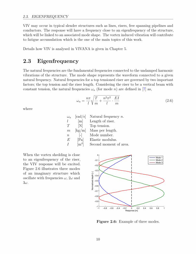
Figure 2.6: Example of three modes.
When the vortex shedding is closeto an eigenfrequency of the riser,the VIV response will be excited.Figure 2.6 illustrates three modesof an imaginary structure whichoscillate with frequencies ω, 2ω and3ω.
10

CHAPTER 2. VIV
2.4 Excitation forceThe force creating the CF vibration is called the dynamic lift force, or the CF excitationforce. It is given by the equation
Fe,CF = 12ρCe,CFDU
2dl (2.7)
where
ρ [kg/m3] Fluid density.Ce,CF [–] Cross flow excitation coefficient.D [m] Structure diameter.U [m/s] Current velocity.dl [m] Length of a small section of the structure.
The excitation coefficient is traditionally mentioned as the lift coefficient in VIV literature.It is defined as the component of the hydrodynamic force that is in phase with the cross flowvelocity of the structure. The value can be positive, which means that energy is added to themotion. The coefficient can also be negative which will lead to damping. This is easy to seefrom Figure 2.5, where the amplitude of the motion first increases until a certain value andthen gets smaller. This implies that the excitation coefficient is dependant on the responseamplitude. In VIVANA, the empirical lift coefficient curve is defined as illustrated in Figure2.7.
CL
A/DA/DCL=0A/DCL,max
C
B
A
CL,max
CL,A/D=0
Figure 2.7: Empirical lift coefficient curve.
2.5 Free oscillation testTo understand how VIV works, experiments need to be done that can help us understand thephysics of the phenomenon. One of these experiments is called the free oscillation test. The
11

2.5. FREE OSCILLATION TEST
free oscillation test is performed by having an elastically supported rigid cylinder in constantcurrent. When the current acts on the cylinder it will force the pipe to vibrate. When thesetest are performed, three different frequencies are found.
The still water frequency
f0 = 12π
√k
m+ma0(2.8)
where
k [N/m] Spring stiffness.m [kg] Mass of the structure.ma0 [kg] Added mass.
The vortex shedding frequency
fv = St · UD
(2.9)
The terms in the equation are explained in Section 2.2.
The oscillating frequency
fosc = 12π
√k
m+ma0(2.10)
where the added mass is valid for the actual flow and oscillation condition.
It is noticed that the oscillation frequency is not identical to the eigenfrequency in still watersince the added mass changes depending on the flow and oscillation conditions. The addedmass is defined as the component of the hydrodynamical force that is in phase with the CFacceleration of the structure. There is a possibility for negative added mass, which is only aconsequence of the phase between the motion of the pipe and the total hydrodynamic force.By performing free oscillation tests of rigid cylinders it is possible to get information aboutparameters such as
• Cross-flow amplitudes and frequencies.
• In-line amplitudes and frequencies.
• Drag coefficient for an oscillating cylinder.
When the tests are performed it is possible to measure the forces acting on the cylinder.The added mass as a function of reduced velocity may also be found. It is important tonote that CF and IL excitation coefficients cannot be found during this type of test becausethey are zero during the free oscillation. One way of dealing with that is to perform forcedoscillation tests. In this way a complete set of coefficients for any combination of frequencyand amplitude may be obtained.
12

CHAPTER 2. VIV
2.6 Forced oscillation testThis test is performed by oscillating a cylinder in a stationary and uniform flow with prescribedmotions. These motions may be harmonic motions in CF and IL direction, or a combinationof these. Examples of CF and IL motion may be,
x = x0sin(4πωosct− ε)y = y0sin(2πωosct)
(2.11)
where
x and y [m] Motions in IL and CF directions.x0 and y0 [m] Amplitudes of IL and CF.ω [rad/s] Oscillating frequency.t [s] Time.ε [rad] Phase angle between IL and CF.
When oscillating the pipe, as described by the equations above, the path of the cross-sectionwill be an eight-figured motion as illustrated in Figure 2.2 and 2.8. The forces can thenbe measured and by processing the data, one can identify force components that are inphase with the forced motion accelerations and velocities in the CF and IL direction. Itis then possible to find the added mass, lift, drag and dynamic force coefficients of the cylinder.
An example of what happens when there is a phase angle between the CF and IL motion isalso illustrated. The equations from above were used to create Figure 2.8.
−0.4 −0.3 −0.2 −0.1 0 0.1 0.2 0.3 0.4−0.4
−0.3
−0.2
−0.1
0
0.1
0.2
0.3
0.4
(A/D
) CF [−
]
(A/D)IL
[−]
Phase angle = 0
Phase angle = π/4
Uniform current
Figure 2.8: Examples of CF + IL trajectory.
13

2.7. ADDED MASS
The results from the forced motion test are usually presented as contour plots for thecoefficients in a non-dimensional amplitude/frequency plane.
Non dimensional
frequency.
Am
plitu
de
ratio, (A
/D
)
Figure 2.9: Contour plot of CF coefficient. Courtesy of Larsen (2011)
Figure 2.9 illustrates the CF excitation coefficient for tests done by Gopalkrishnan [8]. Thesecoefficients are often applied in empirical methods to calculate the response in CF direction.IL motions are known to influence the CF response, however, it is still reasonable to usethe CF coefficients since the CF response is less sensitive to the response in its orthogonaldirection than IL is [6]. The values between 0.125-0.3 [-] are used in the VIVANA software.It means that all eigenfrequencies that give a non-dimensional frequency between these twovalues are taken as response frequency candidates.
2.7 Added mass
When a structure becomes excited by vortex shedding in a current that is not uniform, theadded mass will vary along its length. The response frequency will appear as an eigenfrequencythat is influenced by this added mass distribution. However, since added mass depends onthe frequency, the correct distribution of added mass cannot be found directly. Consistencybetween the frequency and added mass distribution must therefore be obtained throughan iterative process for each response frequency candidate. In this work the added masscoefficient value has been set to a constant value of 0.8. This is done after a discussion withthe supervisor. Choosing this value gives the best prediction for high mode VIV (prof. C. M.Larsen, pers. comm).
The positive outcome by choosing a constant value of the added mass, is that iteration isunnecessary to find consistency between the correct added mass and the response frequency.This leads to much shorter computation time. Both methods have been tried out in thiswork, and the computation time went from 20 to 2 minutes per simulation.
14

CHAPTER 2. VIV
2.8 Suppression of VIVThere are several ways of reducing the vibrations from vortex shedding. One way to avoidVIV is by not being in the resonant area. This is possible if the highest Strouhal frequencyfor the cross section is lower than the first natural eigenfrequency. Being a great deal abovethe resonant area is complicated. This is because there will always be a higher natural modethat corresponds with to the vortex shedding frequency [9].
Another way of reducing the response is to add suppressing devices to the riser. Examplesare fairing or helical strakes attached to the riser as illustrated in the following figure.
x
y
z Pitch
Height
Figure 2.10: Riser with helical strakes.
2.9 Time and space sharingThe characteristics of the VIV response for long, slender structures subjected to a non-uniform current are complicated, and difficult to model. It is observed that the responseof the structure will be a mixture of different modes and frequencies. This response willchange its characteristics with varying current profile, order of dominating modes, influencefrom tension and bending stiffness, mass ratio, Reynlds number and most probably otherparameters as well [6]. There is no model today that can take all of these effects into accountand replicate the response that has been observed. The approach that has been used, is todefine an excitation zone for a specific frequency that is initiated, and calculate the responseof it independently of other active frequencies. The key has been to define this excitationzone. Two different approaches exist. They are called
Time sharing: The competing frequencies will dominate one period of time. Since there isa set of frequencies, the domination will shift. The analysis needs a way of finding therelative duration for each competing frequency.
Space sharing: When using the space sharing option, all frequencies will act simultaneously,but every frequency will have a designated length where they are excited. This meansthat the structure length will be shared among the set of response frequencies that areacting.
15

2.9. TIME AND SPACE SHARING
0.125 0.3
1
2
3
45
Zone for
freq. 3.
Zone for
freq. 2.
Zone for
freq. 1.
Non dimensional
frequency.
UN(z)
Figure 2.11: Excitation zones for space sharing frequencies.
In Figure 2.11, it is illustrated how the excitation zones are defined when using space sharing.It is seen that some zones overlap each other. This means that the excitation zones may bedifferent between space and time sharing, something which will give an effect on the fatiguedamage. The zones are defined by specifying an active interval for the non-dimensionalfrequency. They are then ranked by using an energy criterion given as
Ei =∫Le,i
U3(z)D2H(z)
(A
D
)Ce=0
dz (2.12)
The excitation parameter is integrated over the excitation zone for every frequency. The(A/D)Ce=0 is the non-dimensional amplitude where the excitation coefficient shifts from apositive to negative value. This is shown as point C in Figure 2.7.
The time sharing process is shown in the following figure. It is illustrated how the frequenciescompete over the time.
Time
Frequency
freq. i+1
freq. i
freq. i-1
Figure 2.12: Time sharing process.
16

CHAPTER 2. VIV
The same energy criterion is used to rank the response frequencies, and the duration of eachfrequency is found by
Ti = T · Ei∑kn=1En
(2.13)
where
Ti [s] Time duration of response frequency i.T [s] Total time.En [m7/s3] Excitation parameter for frequency n.
In time sharing, the response frequencies will be active over their entire excitation zone.However, they will not be active at the same time. The excitation zones for time sharing areillustrated in Figure 2.13.
0.125 0.3
1
2
3
45
Non dimensional
frequency.
1
2
3
4
UN(z)
Figure 2.13: Excitation zones for time sharing frequencies.
17


Chapter 3Soil Interaction
3.1 IntroductionOne of the great challenges with SCR design is the assessment of fatigue damage due torepetitive loading over the lifetime of the riser. This depends significantly on the assumedpipe–soil interaction behaviour at the location where the riser reaches the seabed surface.This is generally known as the touchdown zone. There is still considerable uncertainty overthe riser–soil mechanics in this region and it is of major concern to the offshore industry.The pipe–soil interaction response is dependant on a range of parameters, such as seabed soilstrength, loading conditions and pipe displacement magnitude. At the touchdown area theriser is typically modelled as a riser with a series of springs [10] as shown in figure 3.1.
A
Seabed B
wa
ua
rota
Maximum depth
of penetration
Initial depth
of penetration.
Springs engaged.Springs not engaged.
wb = 0
rotb = 0
Figure 3.1: Touchdown zone interaction.
19

3.2. PIPE–SOIL RESPONSE
As the riser is laid, it will penetrate a certain distance into the seabed. The enhancedembedment is a consequence of two effects which occur during pipe laying.
• Concentration of pipe-soil contact stress in the touchdown zone.
• The dynamic motion of the pipe.
A distance from the TDP, point B on Figure 3.1, the curvature will become zero and thevertical displacement relative to the initial penetration will also be zero. The loads on theriser are initiated by the motion of the floater and the ocean current acting on the riserstructure. They will result in cyclic rotations as well as vertical and horizontal displacementsat a location above the seabed. This can be seen in Figure 3.1 as point A.
3.2 Pipe–soil responseHodder and Byrne investigated the pipe–soil response between point A and B [11]. They didan experiment on the pipe–soil interaction in a long flume at the Oxford University. There,it was possible to have a bed of soil that was fully liquefied. On the pipe they tested, anactuator was installed on one end to apply specified displacements at point A. The actuatorwas controlled by a computer that made it possible to move the pipe end with either a con-stant velocity, or cyclically in the form of sine waves with different amplitudes and frequencies.
To compare the pipe–soil interaction force experienced by an element of pipe during theexperiment with a numerical model, it was necessary to quantify the distribution of thevertical soil reaction throughout the touchdown zone. To create an appropriate form of thedistribution of the soil bearing pressure below the riser model, a simple numerical model wasconstructed using the finite element program ABAQUS. The model allowed for a comparisonbetween the numerical and experimental results. The soil was modelled as a series of linearsprings at discrete nodes that were able to be released if the pipe was lifted above the soilsurface. It was crucial to model the pipe that way, since disabling the pipe to be lifted wouldhave given extra stresses in the area.
20
CHAPTER 3. SOIL INTERACTION
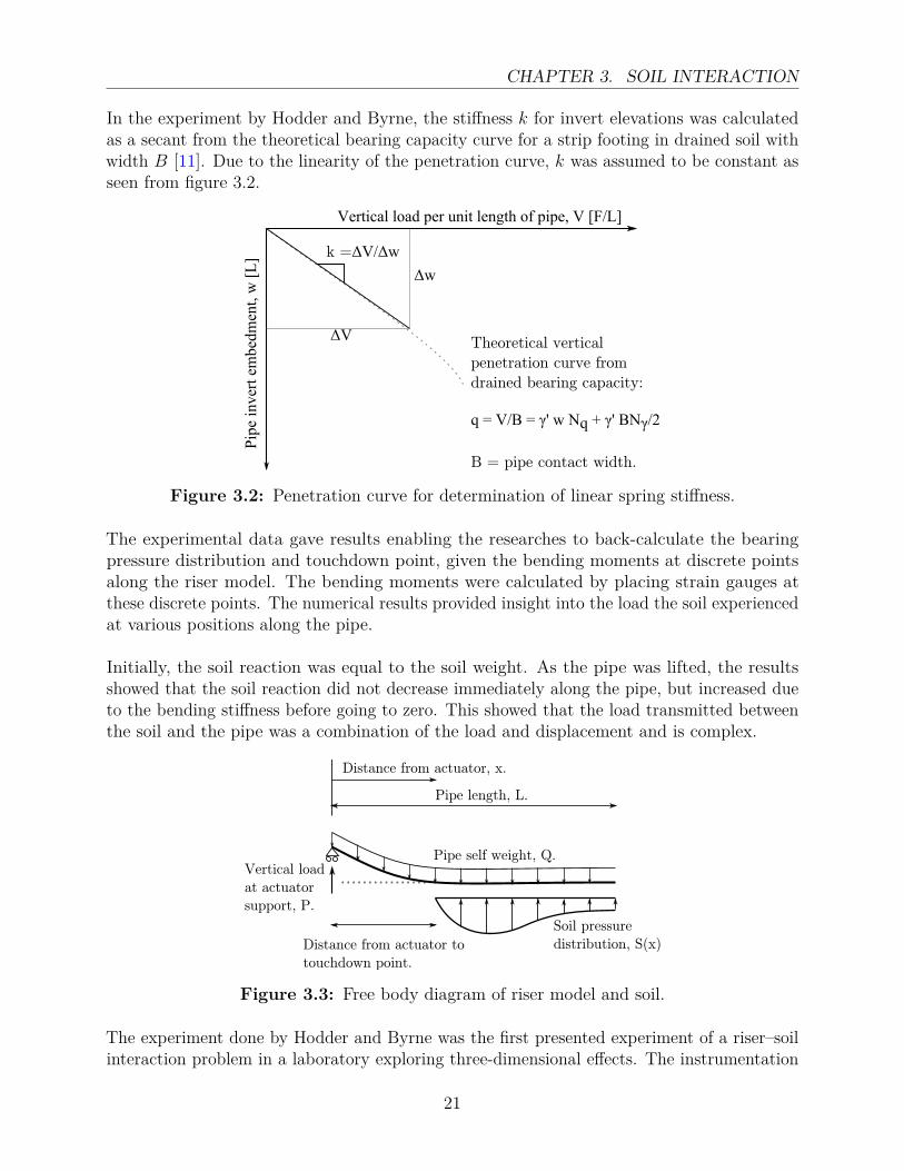
In the experiment by Hodder and Byrne, the stiffness k for invert elevations was calculatedas a secant from the theoretical bearing capacity curve for a strip footing in drained soil withwidth B [11]. Due to the linearity of the penetration curve, k was assumed to be constant asseen from figure 3.2.
Pip
e in
vert
em
bedm
ent,
w [
L]
Vertical load per unit length of pipe, V [F/L]
k =ΔV/Δw
Theoretical vertical
penetration curve from
drained bearing capacity:
q = V/B = γ' w Nq + γ' BNγ/2
B = pipe contact width.
ΔV
Δw
Figure 3.2: Penetration curve for determination of linear spring stiffness.
The experimental data gave results enabling the researches to back-calculate the bearingpressure distribution and touchdown point, given the bending moments at discrete pointsalong the riser model. The bending moments were calculated by placing strain gauges atthese discrete points. The numerical results provided insight into the load the soil experiencedat various positions along the pipe.
Initially, the soil reaction was equal to the soil weight. As the pipe was lifted, the resultsshowed that the soil reaction did not decrease immediately along the pipe, but increased dueto the bending stiffness before going to zero. This showed that the load transmitted betweenthe soil and the pipe was a combination of the load and displacement and is complex.
Soil pressure
distribution, S(x)
Pipe self weight, Q.
Distance from actuator, x.
Pipe length, L.
Vertical load
at actuator
support, P.
Distance from actuator to
touchdown point.
Figure 3.3: Free body diagram of riser model and soil.
The experiment done by Hodder and Byrne was the first presented experiment of a riser–soilinteraction problem in a laboratory exploring three-dimensional effects. The instrumentation
21

3.3. DYNAMIC INTERACTION OF CATENARY RISERS WITH THE SEA FLOOR
was used to quantify riser performance, trench formation and the development of excesswater/pore pressure. The results showed that it was possible to back-calculate an estimateof the touchdown point and the distribution of the soil reaction that occurred during theexperiment.
3.3 Dynamic interaction of catenary risers with the seafloor
Another study was done by Katifeoglou and Chatjigeorgiou [12] on the dynamic interactionbetween a catenary riser and the sea floor. They made a global dynamic behaviour of aSCR. The sea floor–structure phenomenon was given particular attention. The geotechnicalcomputations showed an amplification of the reaction force with the depth of penetrationand the arc of the contact edge. They made several assumptions due to the uncertaintieswith the interaction problem. The numerical experiments they performed showed that theprimarily affected component, the bending moment, was the most sensitive factor for fatigue.
22

Chapter 4
Fatigue
4.1 Introduction
Fatigue occurs when a material is subjected to a loading and unloading which is of repetitivenature. If these loads are above a certain limit, there will be an initiation of microscopiccracks. When the crack growth is allowed to proceed, the structure may suddenly fracture.The cyclic load that is applied on the structure and which initiates the fatigue is less thanthe ultimate tensile stress limit, and may be below the yield stress limit of the material.Examples of cyclic loading important to offshore structures can be loading from waves, or asin this work, loading induced by vortex shedding.
4.2 SCR fatigue design
Fatigue damage is normally estimated by using either S-N curves or fracture mechanics.Today, almost all fatigue analyses of SCRs are performed using S-N curves [13]. When usingS-N curves, the fatigue damage is estimated by using the Palmgren-Miner rule summation asshown in Equation 4.14. The S-N curves form the basis for description of the SCR fatiguecapacity. The curves relate the number of stress cycles to failure to the corresponding stressrange including the effects of stress concentration factors (SCF). The relevant S-N curveapplicable to risers have either a single slope or a two-slope (bilinear) behaviour. The singlesloped curve, which is mostly used can be expressed as
N = a · S−k (4.1)
where a and k are parameters defining the curve which are dependant on the material anddetails obtained from fatigue experiments. S is the stress range. Most of the S-N data arederived by fatigue testing of small specimen in test laboratories. For simple test specimens,the testing is performed until the specimens have failed. In these specimens there is nopossibility for redistribution of stresses during crack growth. This means that most of thefatigue life is associated with growth of a small crack that grows faster and faster as the cracksize increases until fracture [14].
23

4.3. SELECTION OF SN CURVE
4.3 Selection of SN curveFrom [14] we know that for practical purposes, welded joints are divided into several classes,where each class has its own S-N curve. Tubular joints such as risers are assumed to beclass T. Other types of joints, including tube to plate, may fall in one of the other 14 classesdefined in the recommended practice (RP-C203). Each construction detail where fatiguecracks potentially may develop should be placed into its relevant joint class. In any weldedjoint, there are several locations at which the fatigue crack may develop. This may be at theweld toe in each of the parts joined, at the weld ends and at the weld itself. Each locationshould be classified separately.
The basic design SN curve is given as
log(N) = log(a)−m · log(∆σ) (4.2)where
N [–] Predicted number of cycles to failure for stress range ∆σ.∆σ [MPa] Stress range.m [–] Negative inverse slope of SN curve.log(a) [–] Intercept of log N-axis by SN curve.
The fatigue strength is somewhat dependant on the plate thickness. This effect is determinedby the local geometry of the weld toe in relation to the thickness of the adjoining plates.The thickness effect is accounted for by a modification of the stress such that the design S-Ncurve for thickness larger than the reference thickness is given by
log(N) = log(a)−m · log∆σ
(t
tref
)k (4.3)
where
tref [mm] Reference thickness is 25 [mm] for welded connections other thantubular joints. For tubular joints the reference thickness is 32[mm]. For bolts, the thickness is 25 [mm].
t [mm] Thickness through which a crack will most likely grow. t = trefis used for thicknesses less than the refernese thickness.
k [–] 0.1 for tubular butt welds made from one side.
24

CHAPTER 4. FATIGUE
An example of a single sloped S-N curve is illustrated in Figure 4.1. The S2-value is the stressvalue that after 107 cycles with the indicated stress, will give fracture. It is also seen that ahigher stress value will need a smaller number of cycles to fracture.
104 105 106 107 108 109
S1
S2
Str
ess
Am
plitu
des
(lo
g s
cale
) , S
Cycles to failure (log scale), N.
1
m
Figure 4.1: Example of SN curve
In general the thickness exponent is included in the design equation to account for a situationwhere the actual size of the structural component considered is different in geometry thanthe S-N data are based on. To some extent it also accounts for the size of the weld and theattachment. However, it does not account for weld length or length of components differentfrom the ones tested. An example is a mooring system where the number of chain links in theactual mooring are significantly larger than in the test case. The size effect should thereforebe carefully considered using probabilistic theory to achieve reliable design.
25

4.4. EFFECT OF FLOATER TYPE ON SCR FATIGUE
4.4 Effect of floater type on SCR fatigueTypical SCR fatigue analyses include first order and second order floater motion inducedfatigue, VIV fatigue, deep draft floater vortex induced motion (VIM) fatigue, slugging fatigue,fatigue accumulated by start-up and shut-down, installation and other kinds of dynamicloading imposed to the SCR [13].
Depending both on the geographical location and floater type, the fatigue damage might alsovary from one floater concept to another. The author from [13] listed in his article whichprimary factors to fatigue are of great interest for different vessel types.
TLP SEMI SPAR FPSO
Figure 4.2: Examples of offshore drilling types.
• SPAR buoy: VIM fatigue.
• Semi-submersible: Motion fatigue and heave induced VIV fatigue.
• Deep draft semi-submersible: Motion fatigue and VIM fatigue.
• TLP: Motion Fatigue.
• FPSO: Motion fatigue.
4.5 Fatigue Reliability AnalysisFatigue design of a steel catenary riser at the touchdown point is a challenging problem. Oneof the greatest challenges is the fatigue assessment near the touchdown point. The TDP willoften experience the worst cyclic loads, is inaccessible for inspection and is subjected to manyuncertainties.
Even though there have been several advancements in the development of realistic soil models,there are still many uncertainties because of the complexity of soil mechanisms. Someexamples are that models are built on idealized loading sequences which may not represent
26
CHAPTER 4. FATIGUE
what is encountered by a riser. Another example is that empirical coefficients have not beenestimated to precision, since they are obtained from specific soil conditions. Acquisition ofactual site data might be difficult, especially in great depths. Another problem is how thetouchdown point is effected by vortex induced vibrations. Because of the uncertainties inriser fatigue analysis, a safety factor of 10 is recommended on the predicted fatigue life forcritical structural components [15].
Li and Low [16] did a reliability analysis to find what parameters were of importance forfatigue assessment. They were motivated to do this due to the lack of fatigue reliabilityanalysis that addressed the seabed uncertainties. It was important for the researchers toidentify the critical parameters that contributed to the uncertainty of fatigue damage. Thiswas succeeded by characterizing the probability distributions of the parameters, somethingwhich was not straightforward. In their research they used a fatigue methodology that wasbased on a S-N curve that relates the stress range to the number of cycles to failure. Forirregular stress, the rainflow counting algorithm was used, and the Palmgren-Miner rule wasused to sum up the total damage.
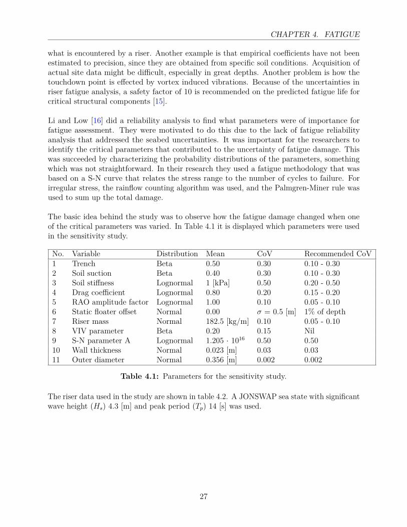
The basic idea behind the study was to observe how the fatigue damage changed when oneof the critical parameters was varied. In Table 4.1 it is displayed which parameters were usedin the sensitivity study.
No. Variable Distribution Mean CoV Recommended CoV1 Trench Beta 0.50 0.30 0.10 - 0.302 Soil suction Beta 0.40 0.30 0.10 - 0.303 Soil stiffness Lognormal 1 [kPa] 0.50 0.20 - 0.504 Drag coefficient Lognormal 0.80 0.20 0.15 - 0.205 RAO amplitude factor Lognormal 1.00 0.10 0.05 - 0.106 Static floater offset Normal 0.00 σ = 0.5 [m] 1% of depth7 Riser mass Normal 182.5 [kg/m] 0.10 0.05 - 0.108 VIV parameter Beta 0.20 0.15 Nil9 S-N parameter A Lognormal 1.205 · 1016 0.50 0.5010 Wall thickness Normal 0.023 [m] 0.03 0.0311 Outer diameter Normal 0.356 [m] 0.002 0.002
Table 4.1: Parameters for the sensitivity study.
The riser data used in the study are shown in table 4.2. A JONSWAP sea state with significantwave height (Hs) 4.3 [m] and peak period (Tp) 14 [s] was used.
27

4.5. FATIGUE RELIABILITY ANALYSIS
Parameter Value Parameter ValueRiser length [m] 1 700 I [cm4] 3.467 · 104
Outer diameter [mm] 356 E [N/m2] 2.1 · 1011
Wall thickness [mm] 24 CD 0.8Mass [kg/m] 182.5 CM 1.8Area [cm2] 250.3 Hang off angle [◦] 14
Table 4.2: Riser data in parameter study
After running analyses with the computer program OrcaFlex, the authors were able to seehow the different parameters effected the riser. The data showed that:
• The seabed variables were influential at the TDP. The reason was that the seabedmodel acted as a boundary condition. The authors meant that this was critical to thestructure near the boundary, and did not effect the global SCR response.
• The static offset was another variable that had great influence near the TDP. This wasexplained by that the offset modified the riser configuration at the seabed.
• The middle section was mostly affected by the drag coefficient and the riser mass, whichcontrolled the damping and the natural frequencies.
• The response amplitude operator (RAO) and VIV had the most effect at the top. TheRAO controls the vessel motions, and the current is largest at the surface. They sawthat near the TDP, "cushioning" of the seabed tended to buffer the changes in theloading condition.
• The S-N parameter showed most variability in the fatigue damage. However, theseuncertainties are generally accounted for in fatigue design, the authors explained.
• The wall thickness and outer diameter had negligible effect on the damage uncertainty,and they are also easy to determine.
• The result showed that the fatigue damage increased with soil stiffness, since soft soilwould distribute the stress over a longer section.
• The trench depth was favourable for the fatigue since it allowed for a more naturaltransition for the riser.
• The soil suction showed an negative effect. This was due to the extra loads on the riserduring uplift from the trench.
The authors made a table showing where each parameter had its main effect. In this way,they were able to set a category on the parameters. The categories were seabed, general anddeterministic.
28

CHAPTER 4. FATIGUE
Variable CoV of fatigue damage CategoryTDP On top Middle partTrench 0.090 0.002 0.003 SeabedSoil suction 0.088 0.003 0.004 SeabedSoil stiffness 0.156 0.004 0.008 SeabedDrag coefficient 0.066 0.089 0.06 GeneralRAO amplitude factor 0.081 0.041 0.033 GeneralStatic floater offset 0.314 0.442 0.298 GeneralRiser mass 0.512 0.511 0.512 GeneralVIV parameter 0.051 0.038 0.201 GeneralS-N parameter A 0.084 0.187 0.258 GeneralWall thickness 0.003 0.004 0.003 DeterministicOuter diameter 0.001 0.007 0.007 Deterministic
Table 4.3: Results from the sensetivity study.
4.6 Fatigue Analysis in VIVANA
4.6.1 Introduction
VIVANA calculates the fatigue damage assuming that the cross section is circular with adiameter defined from the cross section data from SIMA. This is given in the input filesima_inpmod.inp. The stresses are calculated on the outer surface.The method for calculating the fatigue depends on the analysis options which are presentedin the table below.
Fatigue analysis: VIV analysis option:Pure IL Pure CF Combined CF and IL
Space sharing 1 1 1Time sharing 2 2 3
Table 4.4: VIVANA methods for fatigue calculation
The numbers in the table above are explained by the following.
1. Generation of time histories, rainflow counting.
2. Closed form solution.
3. Closed form solution (Gouyang 1989).
In this work, only CF has been investigated and space sharing has been used. This meansthe rainflow counting is used (option 1).
29

4.6. FATIGUE ANALYSIS IN VIVANA
4.6.2 Generation of time seriesWhen the VIV analysis is finished, there are N complex response vectors xi, where i = 1 . . . N .By using them in combination together with the element stiffness matrices and the crosssection properties, one can get time series of the stress at the element ends. The stress cyclesare counted by the rainflow method and the fatigue damage is found by the Palmgren-Minersummation.
The procedure follows these steps.
1: Complex vectors of element forces for all elements at all response frequencies are calculatedby
si,iel = kiel · xi,iel (4.4)
Where i = 1, 2 . . . , N and iel = 1, 2 . . . , Nelements. kiel is the element stiffness matrix and xi,ielcontains the components from the total x-matrix, and represents the local degrees of free-dom to element iel. The dimension of the different components is; s and x is 12×1, k is 12×12.
2: The stresses at the element ends are found by
σi,iel,iend,ipt = piel,iptsi,iel,iend (4.5)
ipt = 1, 2, . . . , Npt and iend = 1, 2. si,iel,iend is a vector of dimension 6 at each end of theelement (iend = 1 and iend = 2). piel,ipt is a vector of dimension 6 containing the crosssection properties of the element and Npt is the number of places on the cross section thatneeds to be checked for fatigue. piel,ipt is given by
piel,ipt =[SCFAXAst,iel
0.0 0.0 0.0 SCFMYWy,iel,ipt
SCFMZWz,iel,ipt
](4.6)
where
Wy,iel,ipt = Wy,iel
sin· (2π · ipt
Npt
) (4.7a)
Wz,iel,ipt = Wz,iel
cos· (2π · ipt
Npt
) (4.7b)
Ast,iel is the cross section steel area and Wy/z are the section modulus for bending about they- and z-axis. SCFAX, SCFMY and SCFMZ are stress concentration factors for axial tension,bending about local y-axis and bending about local z-axis.
3: The stresses at the elements are represented as complex numbers, and the time series ofthe stress can be written as a summation of the contributions from all response frequencies,
σiel,iend,ipt(t) =N∑i=1
σi,iel,iend,ipt · ei(ωit+εi) (4.8)
30

CHAPTER 4. FATIGUE
ωi is the response frequency number i, and εi is the phase angle at the respective frequencyand is a random number between 0 and 2π.
The complex number can be written as
σ = σRe + iσIm (4.9)In the end, the stresses are given by
σiel,iend,ipt(t) =N∑i=1
σamp,i,iel,iend,ipt · cos(ωit+ θi,iel,iend,ipt + εi) (4.10)
where
σamp,i,iel,iend,ipt =√σ2Re,i,iel,iend,ipt + σ2
Im,i,iel,iend,ipt (4.11)
θi,iel,iend,ipt = atan(σIm,i,iel,iend,iptσRe,i,iel,iend,ipt
) (4.12)
4: In this step, a time series of length T [s] is generated. Then one has to define a number ofstress ranges ∆σi, where i = 1, 2, . . . , N∆σ. The rainflow counting method is then used forfinding the number of occurrences for each cycle ni,iel,iend,ipt.
The total number of cycles for stress range i during one year is then calculated as
ni,year,iel,iend,ipt = ni,iel,iend,ipt · 365 · 24 · 60 · 60T
(4.13)
The accumulated damage is then calculated by the Palmgren-Miner sum:
Diel,iend,ipt =N∆σ∑i=1
ni,year,iel,iend,iptNi
(4.14)
Ni is the number of cycles to failure for stress cycle i, and may be found by use of thefollowing equation
logNi = logC +m · log
∆σ ·(tieltref
)k (4.15)
logC,m, tref and k are found from the S-N curve used in VIVANA, tiel is the wall thicknessfor the cross section and ∆σi is the stress range.
31


Chapter 5Software
This chapter gives a short introduction to the different computer programs used in the thesis.
5.1 SIMA and RIFLEXRIFLEX was developed as a tool for analysis of flexible marine riser systems. However, it iswell suited for other type of slender structures as well. These slender structures are mooringlines, umbilicals, steel pipelines and conventional risers. In the thesis the SIMA program isused to model the SCR riser. SIMA has a graphical interface which helps the user get easilyfamiliar with the software. RIFLEX is used for calculations of the model created in SIMA.RIFLEX gives the user the possibility to calculate the structural response. The program maycompute static and dynamic characteristics of the structure [17].
5.2 SIMOThis computer program was used by the supervisor in DNV that produced the vessel motioncoordinates. Details about SIMO are not given here.
5.3 VIVANAVIVANA is a computer program for evaluation and analysis of vortex induced vibrations inslender marine structures. We know from experience that an ocean current might cause VIVon slender marine structures. VIVANA requires RIFLEX to do a static analysis first. A briefintroduction how VIVANA does its calculations is given in the following section.
33
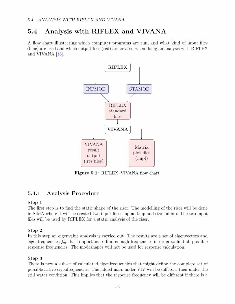
5.4. ANALYSIS WITH RIFLEX AND VIVANA
5.4 Analysis with RIFLEX and VIVANAA flow chart illustrating which computer programs are run, and what kind of input files(blue) are used and which output files (red) are created when doing an analysis with RIFLEXand VIVANA [18].
RIFLEX
STAMODINPMOD
RIFLEXstandard
files
VIVANA
VIVANAresultoutput
(.res files)
Matrixplot files(.mpf)
Figure 5.1: RIFLEX–VIVANA flow chart.
5.4.1 Analysis ProcedureStep 1The first step is to find the static shape of the riser. The modelling of the riser will be donein SIMA where it will be created two input files: inpmod.inp and stamod.inp. The two inputfiles will be used by RIFLEX for a static analysis of the riser.
Step 2In this step an eigenvalue analysis is carried out. The results are a set of eigenvectors andeigenfrequencies f0i. It is important to find enough frequencies in order to find all possibleresponse frequencies. The modeshapes will not be used for response calculation.
Step 3There is now a subset of calculated eigenfrequencies that might define the complete set ofpossible active eigenfrequencies. The added mass under VIV will be different then under thestill water condition. This implies that the response frequency will be different if there is a
34

CHAPTER 5. SOFTWARE
current, than in still water. One must therefore apply iteration for each response frequencycandidate in order to find the actual response frequency. This is because the added massdepends on the frequency and a correct added mass distribution cannot be found directly.The iteration has converged when there is consistency between the modified eigenfrequencyand modified added mass distribution. In this work, the added mass coefficient has been setto a constant value of 0.8 after conversations with the supervisor. The dominating frequencywill be identified according to an energy criteria linked to the integral:
Ei =∫Le,i
UN(z)2DH(z)3(A
D
)Ce,CF=0
dz (5.1)
The frequency with the highest numerical value is chosen. (AD
)Ce,CF=0 is the non-dimensionalamplitude that gives zero dynamic lift force. All eigenfrequencies that have a zone along thestructure with fi (non-dimensional frequency) between 0.125 - 0.3 [Hz] are taken as responsefrequencies. Figure 5.2 shows five different non-dimensional frequency candidates. However,only four of them are within the zone. This is seen by the red color. The non-dimensionalfrequency changes along the depth because the current velocity changes (see equation 5.2).
0.125 0.3
1
2
3
45
Non dimensional
frequency.
Min MaxUN(z)
Figure 5.2: Response frequencies.
The non-dimensional frequency is given as
f = foscD
U(5.2)
where fosc is the oscillation frequency. D and U are two parameters that may vary alongthe length of the riser. This is because all coefficients depend on the non-dimensionalfrequency[19]. The reason why f = 0.125− 0.3 [-], is beacuse of Gopalkrishnan’s tests from1993 with forced CF motions of a rigid cylinder [8]. He found that a positive excitationcoefficient was in this interval for the non-dimensional frequency.
Step 4To analyse the response at the dominating frequencies calculated in step 3, the frequencyresponse method is used. An iteration is applied and it converges when the response is in
35

5.4. ANALYSIS WITH RIFLEX AND VIVANA
accordance with the non-linear models for excitation and damping. The reason for usingiteration is because the lift and damping coefficient depend on the local response amplitude,(A/D). A part of the iteration is to have correct phase between the lift force and responseat all locations on the riser. The frequency response method is well suited for this kind ofcalculation since the loads are assumed to act at known, discrete frequencies. By using finiteelements and the frequency response method, the dynamic equilibrium may be written as
Mr + Cr + Kr = R (5.3)
where M is the mass matrix, C is the damping matrix and K is the stiffness matrix. r is thedisplacement vector. By differentiating the latter once and twice, one will get the velocityand acceleration vector. The external load is harmonic, but loads at all degrees of freedomare not necessarily in phase. It is therefore convenient describing this type of load pattern bya complex load vector X that has a harmonic time variation at a known frequency ω. Theload vector is defined as
R(t) = Xeiωt (5.4)
The phase of the load at a specific degree of freedom is defined by the relative magnitude ofthe real and and imaginary components of the associated element in the complex load vector,equation 5.4.The response vector is also a complex vector with a harmonic time variation. It is defined as
r(t) = xeiωt (5.5)
By inserting the response vector in equation 5.3 and then using equation 5.4, we will get
− ω2(MS + MH)x + iω(CS + CH)x + Kx = X (5.6)
where
MS Structural mass matrix.MH Hydrodynamic mass matrix.CS Sstructural damping matrix.CH Hydrodynamic damping matrix.X Excitation force vector. Non-zero terms are present
within an excitation zone. The excitation force mustalways be in phase with the local response velocity.
Step 5When the responses are known it is possible to calculate the fatigue damage. A user definedS-N curve and the Palmgren-Miner rule is applied. For the space sharing frequencies arainflow counting algorithm is used. For the time sharing option, an analytical solution isused.
36

CHAPTER 5. SOFTWARE
5.5 BATCH-scriptingLearning how to create a BATCH-script has been important in this work to do analyseswith many different parameters. The BATCH-scripts are used to run RIFLEX and VIVANA.Before they are run, the script will get the correct variables from a text-file containingthe relevant information, and these parameters are then inserted into the input files. Theparameters are inserted into variables called wild-cards, and they can be found in the initialinput files. Every wild-card starts with a dollar sign and has a name in capital letters. Anexample is $CURDIR which is the wild-card for the ocean current direction. A part of theINPMOD input file is illustrated below to show how the wild-cards are used.
NEW CURRENT STATE'−−−−−−−−−−−−−−−−−−−−−−−−−−−−−−−−−−−−−−−−−−−−−−−−−−−−−−−−−−−−−−−−−−−−−−'Always remeber that first curlev has to be −0.0 and not 0.0!'icusta nculev1 7
'curlev curdir curvel−0.0 $CURDIR 0.242−10.0 $CURDIR 0.210−50.0 $CURDIR 0.182−200.0 $CURDIR 0.171−500.0 $CURDIR 0.137−1000.0 $CURDIR 0.116−1500.0 $CURDIR 0.000
The variables that are inserted to the wild-cards are found in text-files that the BATCH-scriptloops through. These files are called variations.txt files. More explanation about them canbe found in appendix A.2.
When the correct variables are assigned using the change_str_in_file.m function, the scriptwill active RIFLEX and then VIVANA. When these analyses are finished, the BATCH-script will activate Matlab and use functions and scripts which are created for purposessuch as to plot the data in the matrix plot files created by VIVANA and RIFLEX. Figure5.3 displays a flow chart that illustrates how the BATCH-process is executed and how itcommunicates with the functions created in Matlab. The name of all the BATCH-scriptsused is run_with_matlab.bat. The BATCH-scripts are placed in their respective analysisfolder, where they are executed. Thus, even if the names of several BATCH-scripts usedin this work are the same, the BATCH-scripts may have different functions in the differentfolders. Both BATCH-scripts used in this work are attached in the appendix. This is done inorder to give the reader an better explanation on how the scripts are constructed.
37

5.6. MATLAB
BATCH-script
change_str_in_file.m
riflex.inpand
vivana.inp
RIFLEX
VIVANA
postprocess_mpf.m
run BATCH-script
insert wild-cards to input files
Figure 5.3: Flow chart of a BATCH-process.
This flow chart explains also how the parameter variation analysis was performed.
5.6 MATLABMatlab has been widely used in this master thesis. The main application of the program inthis work has been to
• Create functions that communicate together with the BATCH-script in order to runRIFLEX and VIVANA with different parameters.
• Create plots from the matrix plot file (.mpf) file that VIVANA produces.
• Process the vessel motion coordinates.
• Create necessary plots of the vessel statistics.
• Process results from the parameter variation analysis and variation of vessel coordinateanalysis.
All functions and scripts have been attached in the appendix. They have been uploaded to azip-file to DAIM as well. Every function and script has a small explanation at the beginningto help the user understand how they are used.
38

CHAPTER 5. SOFTWARE
A list of Matlab scripts with a small description is given on the following pages.change_str_in_file.m This function will read a input file and replace the wild-cards with
given parameters.
postprocess_mpf The scripts imports the results from the .mpf-file created byRIFLEX,VIVANA and etc. It creates a struct with the data from the .mpf-file andplots the results in a folder.
read_xy_data.m This Matlab script is created to read through the Xpos.asc and Ypos.asc(from the SIMO analysis) files that contain the data of the vessel motion and save themin a struct for further processing.
find_extreme_coord.m Find the largest extreme coordinates from the data.
transform_xy_data.m The function takes in the original (x, y) data, and transformsthem according to the new transformed coordinate system.
count_in_large_matrix.m This function goes through all the transformed, multipliedcoordinates, and inserts the number of occurrences into a large matrix.
xy_count_and_prob.m The function goes through all the coordinates in thecounted_x_y_data- matrix and finds the number of occurrences in thelarge_transformed_coord_matrix. By knowing the total number of occurrences it ispossible to find the probability of the motion p(x, y).
convert_xy_to_polar_xy.m This function extracts the coordinates, their counts andprobability, and converts the coordinates to polar coordinates, for further processing.
search_xy_in_sectors.m This function will go through the sectors and the discrete pointsdefined in the input, and count the occurrences of the (x, y) position of the vessel.
extract_fatigue_from_mpf.m This function extracts the fatigue info from the input.mpf-file and creates a new file with only the fatigue data. This is created in order tominimize the space when running the riser analysis with many (x, y) coordinates.
save_run_xy_info_in_struct.m This function goes through all the folders containingthe info of the (x, y) coordinate variation runs and saves it in a struct for furtherprocessing.
add_fatigue_damage_to_struct.m The function goes to the respective folder, andextracts the fatigue damage saved in the fatigue_damage.txt file. It then saves thisinfo in the struct for further processing.
sum_fatigue_damage_from_xy_variation.m The function goes through the run_datastruct and sums the fatigue damage.
find_important_parameters_resfile.m This function finds important parameters fromthe stamod.res file, which contains results from the static analysis of the riser. Thisfunction was created because the large .mpf-files are deleted in the variation of vesselcoordinate analysis due to large data size.
39

5.6. MATLAB
5.6.1 Flow chart for processing the vessel motion dataIn this work, it was necessary to process the vessel motion data given by DNV in orderto create a discrete probability distribution. More info about the motion data is given inSection 8.3. A flow chart is created under to give the reader information of how the datawas processed. The green boxes are I/O files which are in a simple text format. The redboxes are the main Matlab-script which runs the functions beneath them. The blue box isthe BATCH-script.
Xpos.asc Ypos.asc
process_x_y_data.m
find_extreme_coord.m
transform_xy_data.m
count_in_large_matrix.m
xy_count_and_prob.m
convert_xy_to_polar_xy.m
search_xy_in_in_sectors.m
variations.txt
BATCH-script
Fatigue damagefor every vessel
coordinate, (xi, yi).
run_variation.m
save_run_xy_info_in_struct.m
add_fatigue_damage_to_struct.m
sum_fatigue_damage_from_xy_variation.m
Finalfatigueresults
input
output
input
output
fatigue.txt
output
Figure 5.4: Flow chart of Matlab functions used in the variation of vessel coordinateanalysis.
40

Chapter 6Riser configuration
z
x
Riser hang off point.
Touch down point.
Vessel/floater
Steel
Catenary
Riser
Figure 6.1: Riser configuration example, ZX-plane.
(x3,y3)
(x1,y1)
(x2,y2)=(0,0)
Vessel motion.
Riser config. when RHoP at
(x1,y1) and (x3,y3).
Riser config. when RHoP at (0,0).
z
x
Figure 6.2: Riser configuration example, XY-plane.
External diameter [mm] 230.0Wall thickness [mm] 25.4Internal diameter [mm] 179.2Density [kg/m3] 7850.0E-modulus [Pa] 2.00E+11Second moment of area, I [m4] 8.67E-05Mass per length [kg/m] 128.2Axial stiffness [kN] 3.27E+06Bending stiffness [kNm2] 1.73E+04Torsional stiffness [Nm2/rad] 1.00E+05
Table 6.1: Data of the SCR.
41

Figure 6.1 illustrates the configuration of the SCR, and how it was originally modelled inSIMA. The original riser hang off point (RHoP) was set to the origin, and the terminationpoint was set to a value of x = 896.0 [m]. The static shape was originally found by using thecatenary equations given in [20]. Figure 6.1 illustrates the riser seen from the side, where thex-axis points to the right and the z-axis upwards. The figure to the right illustrates the samefloater and riser seen from above. In that figure there are three different positions displayingan example of the vessel motion. When the riser was modelled in SIMA the RHoP was set tothe origin as one can see from the (x2, y2) position above. The data used for modelling theriser have been found after conversations with the supervisor at the department of MarineTechnology, and the co-supervisor from DNV.
42

Chapter 7Parameter variation analysis
7.1 IntroductionA significant effort has been made over the last decades to develop new VIV models orimprove existing ones. However, it is still obvious that deterministic estimates of full scaleriser VIV fatigue damage will include great uncertainties. These uncertainties are mainly dueto the lack of knowledge of the ocean currents generating the VIV and the complex nature ofVIV itself. Much of the uncertainty is linked to the amount and relevance of data availableto understand, characterize VIV and capture the broad complexity of the phenomenon. Inthis master thesis one of the tasks is to find out how different parameters used in the for thefatigue analysis will effect the results.
One of the challenges when doing a parameter analysis is finding which parameters areimportant. In the thesis, the variables that have been tested are assumed to be parameterswhich are difficult to predict precisely and which will have an notable impact on the fatigueresults. The paramters tested in the thesis are displayed in the following.
• Ocean current (only unidirectional).
• Current heading.
• Bottom properties.
• Relative damping.
• Number of elements of second segment.
• S-N curve.
All parameters and their values are displayed in appendix A.2.1.
7.2 Current profile and directionThe current profile in VIVANA can only be modelled unidirectionally. From studies done by[5], this is seen to be unrealistic. The current might vary with the depth, both in magnitudeand direction. The latter is not possible to do with VIVANA at the moment. This is ofcourse a problem, because the vortex shedding is influenced by the current. Another problemwith current modelling, is that it changes direction with time. It is therefore crucial to creategood statistical models of the current which can be used in the analysis.
43

7.3. BOTTOM PROPERTIES
The way this analysis was performed, was to run one analysis with one current at the time.One of the questions when this master thesis was in its starting phase, was to check if it waspossible to use many current profiles, each with its own probability. One would have to doone analysis for each current profile, and in the end, summarize the total damage as
Dtot =N∑i=1
Dcur,i · pcur,i (7.1)
where
Dcur,i [1/yeas] Fatigue damage for current i.pcur,i [-] Probability for current i.
However, only one current profile was used in each analysis, and summation of the damagefrom different current profiles was not done. It has simply been tested how current profileswith different magnitudes and directions effect the fatigue results. The current profile wasmodelled with a velocity distribution with seven points, where each point had a specifiedmagnitude. The values are displayed in Table 7.1.
Current 1 Current 2 Current 3 Current 4Depth [m] [m/s]
0.0 0.242 0.662 1.082 1.478-10.0 0.210 0.545 0.887 1.190-50.0 0.182 0.449 0.726 0.957-200.0 0.171 0.415 0.668 0.866-500.0 0.137 0.306 0.489 0.618-1000.0 0.116 0.247 0.393 0.488-1500.0 0.000 0.000 0.000 0.000
Table 7.1: Current profiles.
The current direction is also of importance when doing the parameter analysis. It is onlypossible to consider four directions with a SCR. This because the CF and IL excitation arenot known for other directions for a SCR since the there will be a coupling effect betweenthe coefficients.
7.3 Bottom propertiesIn VIVANA, the bottom is modelled with springs as bottom stiffness and with dashpots asbottom damping. The starting data (STFBOT = 300.0 [kN], STFAXI = 200.0 [kN] andSTFLAT = 200.00 [kN]) used in the analysis was provided by the co-supervisor from DNV.In this thesis only bottom stiffness has been used in the analysis. The bottom damping hasbeen set to zero. One of the problems with the bottom properties in VIVANA is that infrequency analysis, the springs are not allowed to be released if the riser is lifted from the seafloor. This creates tensile forces which are not realistic. The reason for changing the bottomproperties has been to see how and where the fatigue damage is affected.
44

CHAPTER 7. PARAMETER VARIATION ANALYSIS
7.4 Relative dampingThe relative structural damping is specified by the user when doing the VIV analysis withVIVANA. The relative damping is the internal damping of the structure due to friction andlocal strains. The damping is modelled for each response frequency as a damping matrixproportional to the stiffness matrix [21]
Ci = αiK (7.2)where
Ci Damping matrix for frequency i.K Stiffness matrix.αi Proportionality factor for frequency i.
The damping is known as Rayleigh or proportional damping. It might also include acontribution from the mass matrix as well. From [21] it is found that the inertia part is notneeded since the damping level should be valid for one specific frequency. From standardtheory for structural dynamics, the proportionality factor is given as
αi = 2ξωi
(7.3)
where
ξ User defined structural damping ratio.ωi Response frequency i.
The model used will give the same relative damping contribution for all response frequencies.
7.5 Number of elementsThis parameter was chosen to find out how the FE model in VIVANA converges as thenumber of elements alters. It is only the second segment of the modelled riser that has avarying number of elements. This is also the segment that covers the area where the riserreaches the seabed.
45

7.6. S-N CURVE SELECTION
Segment 1
Segment 2
Segment 3
TDP
Figure 7.1: Riser segments
7.6 S-N curve selectionThe S-N curves relates the number of stress cycles to failure to the corresponding stress range.There exists many S-N curves after numerous tests on structural specimen in laboratories.Still, there is much uncertainty linked to which curve is best fitted for the structure in onesanalyses. How can one know which curve gives the best result? And how does differentcurves effect the final result? The main focus was to figure out how much does the S-N curvechanged the result.
7.7 Info about the resultsEvery parameter tested consist of 3-4 runs. For each parameter varied, four figures aredisplayed illustrating the results. They figures are.
Top left figure: Displaying the fatigue damage of the entire riser for the respective runs.
Top right figure: Displaying the fatigue damage near the TDP area for the respective runs.
Lower left figure: Illustrating the maximum fatigue for every respective run. The valuesare normalized, such that the largest value equals to unity. Used to easily compare themaximum damage and look for trends in the results.
Lower right figure: Illustrating how the point on the structure with maximum fatiguemoves.
46

CHAPTER 7. PARAMETER VARIATION ANALYSIS
7.8 Results
7.8.1 Run 1-4
0 200 400 600 800 1000 1200 1400 1600 1800 20000
0.1
0.2
0.3
0.4
0.5
0.6
0.7
0.8
0.9
1
Norm
aliz
ed fatigue d
am
age [−
]
Max fatigue damage: 0.17 [1/years]
x [m]
run 1
run 2
run 3
run 4
(a) Fatigue damage (whole riser).
1650 1660 1670 1680 1690 1700 1710 1720 1730 1740 17500
0.1
0.2
0.3
0.4
0.5
0.6
0.7
0.8
0.9
1
Norm
aliz
ed fatigue d
am
age [−
]
Max fatigue damage: 0.17 [1/years]
x [m]
(b) Fatigue damage (close to TDP).
run_1 run_2 run_3 run_4
0.1
0.2
0.3
0.4
0.5
0.6
0.7
0.8
0.9
1
1.1Max fatigue: 0.17 [1/years]
Name of analysis.
Norm
aliz
ed f
atig
ue [
Fa
t. d
am
./m
ax(F
at. d
am
.)]
Max fatigue for runi
(c) Max fatigue damage.
1660 1665 1670 1675 1680 1685 1690 1695 1700 1705 1710
run_1
run_2
run_3
run_4
Na
me
of
an
aly
sis
.
Length of riser [m].
Position on the riserwith max fatigue damage.
(d) Riser point with max fatigue.
Figure 7.2: Results from parameter run 1-4.
Run 1-4 is tested with variations in the current magnitude. The values of the current arefound at page 44. The currents have the same form, but are only scaled differently. From theresults in the figures above one can observe that the fatigue damage increases for increasingcurrent velocity. This is an expected result since the number of modes will increase withcurrent velocity, which will give larger curvature and fatigue damage. On the other hand,it is noticed that the maximum fatigue is seen for the third current profile (Run 3). Figure7.2c illustrates this very clearly. By looking at the figure 7.2b and 7.2d it is seen that themaximum fatigue point for the greatest current has a substantial change in position. It seems
47

7.8. RESULTS
that this is caused by the modes excited by the current. This indicates that there may bea connection between which modes are excited and where the maximum fatigue damagewill appear. This is important to notice, because it means that the largest current will notnecessarily give the largest fatigue damage.
There is also an interesting peak around an length of 700 [m]. This can be explained bylooking at the results from the matrix plot file produced by VIVANA. By looking at whichexcitation zones were given to the vortex shedding frequencies, it is clearly seen that theexcitation zone is large in this area, and that the riser will experience largest responseamplitudes here.
The cross flow amplitudes are seen for two frequencies excited, and the excitation zones for alarge part of frequencies are shown. It is illustrated that the greatest response is induced bythe frequency that oscillates with 0.769 [Hz].
0 500 1000 1500 20000
0.01
0.02
0.03
0.04
0.05
0.06
0.07
Arc length (m)
(m)
Response amplitudes, CF
0.769 Hz
0.701 Hz
Figure 7.3: Response amplitudes of Run 4.
0 500 1000 1500 20000
0.2
0.4
0.6
0.8
1
1.2
1.4
Arc length (m)
(Hz)
Excitation zones, part 1
0.769 Hz0.793 Hz0.816 Hz0.939 Hz0.963 Hz0.988 Hz1.013 Hz0.747 Hz1.038 Hz0.724 Hz1.064 Hz1.089 Hz0.701 Hz1.115 Hz1.141 Hz0.679 Hz1.167 Hz0.657 Hz1.194 Hz
0.769 Hz0.701 Hz
Figure 7.4: Excitation zones of Run 4.
48

CHAPTER 7. PARAMETER VARIATION ANALYSIS
7.8.2 Run 5-7
0 200 400 600 800 1000 1200 1400 1600 1800 20000
0.1
0.2
0.3
0.4
0.5
0.6
0.7
0.8
0.9
1
Norm
aliz
ed fatigue d
am
age [−
]
Max fatigue damage: 0.20 [1/years]
x [m]
run 5
run 6
run 7
(a) Fatigue damage (whole riser).
1650 1660 1670 1680 1690 1700 1710 1720 1730 1740 17500
0.1
0.2
0.3
0.4
0.5
0.6
0.7
0.8
0.9
1
Norm
aliz
ed fatigue d
am
age [−
]
Max fatigue damage: 0.20 [1/years]
x [m]
(b) Fatigue damage (close to TDP).
run_5 run_6 run_7
0.7
0.75
0.8
0.85
0.9
0.95
1
1.05
1.1Max fatigue: 0.20 [1/years]
Name of analysis.
Norm
aliz
ed fatigue [F
at. d
am
./m
ax(F
at. d
am
.)]
Max fatigue for runi
(c) Max fatigue damage (Run 5-7).
1702 1704 1706 1708 1710 1712 1714 1716 1718
run_5
run_6
run_7
Na
me
of
an
aly
sis
.
Length of riser [m].
Position on the riserwith max fatigue damage.
(d) Riser point with max fatigue.
Figure 7.5: Results from parameter run 5-7.
49

7.8. RESULTS
In Run 5-7 the current direction is tested. The current magnitude is the same.
Run: Direction [deg]:5 0.06 90.07 270.0
Table 7.2: Current directions used in parameter study.
It is clearly illustrated that the fatigue damage differs depending on which direction thecurrent comes from. This is why it is important to improve existing VIV software to beable to handle all current directions. The difference in fatigue damage is relatively small inthe beginning. This is because the upper part of the riser is quite straight, and the fatiguedamage is similar as for a straight, top tensioned riser. However, the fatigue increases as thecurvature of the riser increases. We can see from the figures above that the current comingin the orthogonal riser plane gives largest fatigue almost over the entire riser, except near theTDP. There, the largest fatigue is seen for Run 5. Run 6 and Run 7 have a maximum fatiguethat is around 84 % and 93 % of Run 5. The point with maximum damage is also differentfor every run in this section. It is also interesting to see that the increase in fatigue damageis quite large for Run 5 and 7 when reaching the touchdown area.
50

CHAPTER 7. PARAMETER VARIATION ANALYSIS
7.8.3 Run 8-11
0 200 400 600 800 1000 1200 1400 1600 1800 20000
0.1
0.2
0.3
0.4
0.5
0.6
0.7
0.8
0.9
1
Norm
aliz
ed fatigue d
am
age [−
]
Max fatigue damage: 0.13 [1/years]
x [m]
run 8
run 9
run 10
run 11
(a) Fatigue damage (whole riser).
1650 1660 1670 1680 1690 1700 1710 1720 1730 1740 17500
0.1
0.2
0.3
0.4
0.5
0.6
0.7
0.8
0.9
1
Norm
aliz
ed fatigue d
am
age [−
]
Max fatigue damage: 0.13 [1/years]
x [m]
(b) Fatigue damage (close to TDP).
run_8 run_9 run_10 run_11
0.7
0.75
0.8
0.85
0.9
0.95
1
1.05
1.1Max fatigue: 0.13 [1/years]
Name of analysis.
Norm
aliz
ed fatigue [F
at. d
am
./m
ax(F
at. d
am
.)]
Max fatigue for runi
(c) Max fatigue damage.
1661.4 1661.6 1661.8 1662 1662.2 1662.4 1662.6 1662.8
run_8
run_9
run_10
run_11
Na
me
of
an
aly
sis
.
Length of riser [m].
Position on the riserwith max fatigue damage.
(d) Riser point with max fatigue.
Figure 7.6: Results from parameter run 8-11.
51

7.8. RESULTS
In Run 8-11 the bottom properties of the sea floor are examined.
Run Bottom stiff. Axial stiff. Lateral stiff.8 300.0 200.0 200.09 250.0 150.0 150.010 200.0 100.0 100.011 150.0 50.0 50.0
Table 7.3: Bottom stiffness values used in the parameter analysis.
All stiffness values are in [kN/m].
The bottom stiffnesses have been minimized with 50 [kN/m] for each run. The results showthat run 8 gave the largest fatigue damage. This was expected as well. There are somedifferences in the fatigue damage before the TDP, however, they are negligible. From Figure7.6a one can notice that Run 10 has a fatigue damage that is not in phase with the otherruns between an arclength of around 600 [m] until somewhere around 1100 [m]. After thatthe damages are in phase with each other. The greatest difference is seen near the touchdownpoint. The run with greatest bottom stiffness gave the worst maximum damage. From theresults, it is seen that the point on the riser with greatest damage does not move considerablywith different bottom properties.
52

CHAPTER 7. PARAMETER VARIATION ANALYSIS
7.8.4 Run 12-14
0 200 400 600 800 1000 1200 1400 1600 1800 20000
0.1
0.2
0.3
0.4
0.5
0.6
0.7
0.8
0.9
1
Norm
aliz
ed fatigue d
am
age [−
]
Max fatigue damage: 0.19 [1/years]
x [m]
run 12
run 13
run 14
(a) Fatigue damage (whole riser).
1650 1660 1670 1680 1690 1700 1710 1720 1730 1740 17500
0.1
0.2
0.3
0.4
0.5
0.6
0.7
0.8
0.9
1
Norm
aliz
ed fatigue d
am
age [−
]
Max fatigue damage: 0.19 [1/years]
x [m]
(b) Fatigue damage (close to TDP).
run_12 run_13 run_14
0.4
0.5
0.6
0.7
0.8
0.9
1
1.1Max fatigue: 0.19 [1/years]
Name of analysis.
Norm
aliz
ed fa
tigue [F
at.
dam
./m
ax(F
at.
da
m.)
]
Max fatigue for runi
(c) Max fatigue damage.
1660 1660.5 1661 1661.5 1662 1662.5
run_12
run_13
run_14
Na
me
of
an
aly
sis
.
Length of riser [m].
Position on the riserwith max fatigue damage.
(d) Riser point with max fatigue.
Figure 7.7: Results from parameter run 12-14.
53

7.8. RESULTS
Run Relative damping Variation12 0.01 Original value13 0.012 +20 % of original value14 0.008 −20 % of original value
Table 7.4: Values of relative damping used in the parameter study.
The results from Run 12-14 were as expected. The riser with the largest relative damping hasthe smallest fatigue damage, and vice versa. However, the results reveal that if the structuraldamping is increased with 20 %, then the maximum damage is decreased with a value ofaround 30 %. If the structural damage is decreased with 20 %, then the maximum fatiguedamage is increased with around 45 %. There is no change of where the maximum fatigueis on the riser. This is satisfactory. The fatigue damages are also in phase, which seemsreasonable.
54

CHAPTER 7. PARAMETER VARIATION ANALYSIS
7.8.5 Run 15-18
0 200 400 600 800 1000 1200 1400 1600 1800 20000
0.1
0.2
0.3
0.4
0.5
0.6
0.7
0.8
0.9
1
Norm
aliz
ed fatigue d
am
age [−
]
Max fatigue damage: 0.13 [1/years]
x [m]
run 15
run 16
run 17
run 18
(a) Fatigue damage (whole riser).
1650 1660 1670 1680 1690 1700 1710 1720 1730 1740 17500
0.1
0.2
0.3
0.4
0.5
0.6
0.7
0.8
0.9
1
Norm
aliz
ed fatigue d
am
age [−
]
Max fatigue damage: 0.13 [1/years]
x [m]
(b) Fatigue damage (close to TDP).
run_15 run_16 run_17 run_18
0.8
0.85
0.9
0.95
1
1.05
1.1Max fatigue: 0.13 [1/years]
Name of analysis.
Norm
aliz
ed fatigue [F
at. d
am
./m
ax(F
at. d
am
.)]
Max fatigue for runi
(c) Max fatigue damage.
1660.4 1660.6 1660.8 1661 1661.2 1661.4 1661.6 1661.8
run_15
run_16
run_17
run_18
Na
me
of
an
aly
sis
.
Length of riser [m].
Position on the riserwith max fatigue damage.
(d) Riser point with max fatigue.
Figure 7.8: Results from parameter run 15-18.
55

7.8. RESULTS
Here are the parameters varied in Run 15-18.
Run No. of elements [-] Element length [m]15 400 2.016 800 1.017 1600 0.518 3200 0.25
Table 7.5: Number of elements used in the parameter study.
The riser is modelled with three segments as illustrated in Figure 7.1. The second segmentis covering the part of the riser which has the greatest curvature and is at the touchdownarea. The total length of the segment is 800 [m]. This is the reason for looking into how finethe elements need to be in this area in order to get reliable results. By looking at Figure7.8a it is not easy to see any differences in the results. However, more details are revealedas the fatigue results are magnified. The maximum fatigue damage is relatively equal forall cases, with only couple of percent difference between each run. The greatest effects ofthe element discretisation is seen at the fatigue top at 1710 [m] in Figure 7.8b. The curve isnot as smooth in the area because of the small number of elements. The two last runs aresmooth and the results satisfactory. In this test case, VIVANA gave quite similar resultseven though the element length was altered between 2.0–0.25 [m].
56

CHAPTER 7. PARAMETER VARIATION ANALYSIS
7.8.6 Run 19-22
0 200 400 600 800 1000 1200 1400 1600 1800 20000
0.1
0.2
0.3
0.4
0.5
0.6
0.7
0.8
0.9
1
Norm
aliz
ed fatigue d
am
age [−
]
Max fatigue damage: 0.83 [1/years]
x [m]
run 19
run 20
run 21
run 22
(a) Fatigue damage (whole riser).
1650 1660 1670 1680 1690 1700 1710 1720 1730 1740 17500
0.1
0.2
0.3
0.4
0.5
0.6
0.7
0.8
0.9
1
Norm
aliz
ed fatigue d
am
age [−
]
Max fatigue damage: 0.83 [1/years]
x [m]
(b) Fatigue damage (close to TDP).
run_19 run_20 run_21 run_22
0.1
0.2
0.3
0.4
0.5
0.6
0.7
0.8
0.9
1
1.1Max fatigue: 0.83 [1/years]
Name of analysis.
Norm
aliz
ed fa
tigue [F
at.
dam
./m
ax(F
at.
da
m.)
]
Max fatigue for runi
(c) Max fatigue damage.
1660 1660.5 1661 1661.5 1662 1662.5
run_19
run_20
run_21
run_22
Na
me
of
an
aly
sis
.
Length of riser [m].
Position on the riserwith max fatigue damage.
(d) Riser point with max fatigue.
Figure 7.9: Results from parameter run 19-22.
The last variable changed in the parameter variation study was different S-N curves, in orderto get an idea of how they effect the final fatigue results. The S-N curves are taken from [14].As mentioned more in detail in Chapter 4, the basic design of a S-N curve is given by theequation
log(N) = log(a)−m · log∆σ
(t
tref
)k (7.4)
where, the log(a) is the intercept of log N-axis by the S-N curve, and m is the negative inverseslope of the S-N curve.
57

7.8. RESULTS
In Run 19-22 the parameters log(a) and m that were changed as found in the recommendedpractice (RP-C203). The values used in this study were:
Run m log(a)19 3 11.76420 4 15.11721 3 12.59222 3 10.970
Table 7.6: S-N curves used in the parameter study.
The results were as expected. When there is a requirement of many cycles to fatigue, as inRun 19 and Run 21, the fatigue is small. This is especially seen for Run 20 where the S-Ncurve is moved up to an intercept of the log N-axis to 15.117. It is easy to notice that thefatigue damage is almost eliminated in this case. On the other hand, the fatigue damage isextremely magnified for Run 22. Here a S-N curve with a low interception is chosen, whichmeans that the number of cycles to fatigue is lowered. This is pointed out in the plots above,where we can see an increase of a great scale in the fatigue damage. The results show thatS-N curves are extremely important to the outcome of the fatigue results.
58

Chapter 8Variation of vessel offset analysis.
8.1 IntroductionThe reason for doing this analysis is because of the strong increase in fatigue damage nearthe TDP of the SCR. A key issue in the design of a SCR is to control stresses and fatiguedamage in the touchdown area. Dynamic bending stresses will vary along the riser, and alarge peak will often be seen near the TDP. The peak is caused by the restrictions on theriser displacement from the presence of the sea floor, and the local bending stresses will beinfluenced by stiffness and damping properties of the bottom.
The analysis model in VIVANA represents the interaction between the riser and the seafloor with discrete springs. In linear frequency domain analysis the spring properties remainconstant independent of the displacements. This type of model may give an over-predictionof the bending stresses at the touchdown point, since a linear spring will induce tensile forcesinstead of being released from the sea bottom when the riser is lifted. The TDP will alsomove with time because of the vessel or floater motion, which will lead to a more distributedfatigue damage (engineer P.E. Voie, pers. comm.).
560 570 580 590 600 610 620 630 640 650−1501
−1500
−1499
−1498
−1497
−1496
−1495
−1494
−1493
−1492
−1491Static config. of the riser at different RHoP (x,y)
x [m]
z−
axis
/ W
ate
r d
ep
th [
m]
Riser hang off coordinate (x,y): (0,0)
TDP
Riser hang off coordinate (x,y): (16.9,0)
TDP
Riser hang off coordinate (x,y): (−24.4,0)
TDP
Figure 8.1: Example of changing TDP.
59

8.2. ANALYSIS STEPS
8.2 Analysis stepsThe analysis of the varying coordinate for the RHoP is going to be explained in the followingpages. Here is a list displaying the overview of the procedure. A flow chart illustrating thisprocedure can be displayed on page 40 as well.
1. Read the vessel motion files with Matlab.
2. Find the largest coordinate values in order to create a transformed coordinate systemwhich only has positive values.
3. Transform the motion coordinates (x, y) into transformed coordinates (XT , YT ).
4. Multiply the transformed coordinates enough such that all coordinates are integers,and then can easily be placed into a matrix.
5. Create a large matrix where the index (i, j) represents the multiplied transformedcoordinates. This is necessary to count the number of occurrences of a original (x, y)coordinate of the vessel motion.
6. Count the occurrences of the transformed coordinates (XT , YT ) into the large matrix.
7. Transform the large coordinates back to the original ones. (XT , YT )⇒ (xi, yi)
8. Having the number of occurrences of each (xi, yi) and the total number of all occurrences,the probability is possible to find by p(xi, yi) = n(xi, yi)/Ntot.
9. There is now a probability p(xi, yi) for each coordinate (xi, yi). Since there are manycoordinates, it is easier to sum the probability of the coordinates into defined discretepoints in sectors that cover all the occurrences.
10. A statistical representation of the vessel motion is described as probability at specifieddiscrete points.
11. An interpolation of the discrete points is carried out in Matlab. This is useful to createa surface and a contour plot of the probability. N.B. The probability is only correcton the surface/contour points corresponding to the discrete points.
12. A RIFLEX and VIVANA analysis is then carried out at each of these discrete points.
13. The fatigue results are extracted into a fatigue.txt file in its respective analysis folder.
14. A Matlab script will sum all the fatigue results with their respective probability inorder to get the final outcome.
15. The final step is comparing the the results from the steps above with the originalanalysis, where the RHoP is placed in origin, and not moved.
60

CHAPTER 8. VARIATION OF VESSEL OFFSET ANALYSIS.
8.3 Vessel motion
8.3.1 Raw data from SIMO analysisThe analysis started with an analysis done by Per Erlend Voie, the co-supervisor from DNV.He did a motion analysis with SIMO of a vessel/platform. The analysis was done usinga scatter diagram of the environmental conditions at a specific area. The details are notimportant in this work. The intention was to get an idea how the fatigue results would beaffected by varying the (x, y) position of the riser hang of point (RHoP). The data that wereanalysed in this work consisted of 556 different folders. Each folder had a specific weathercondition and consisted of two files representing the vessel data. An example of a folder namewas dir0_hs10_tp11.4.
Explanation of the folder name.
dir [degrees] Direction of the weather.h_s [m] Significant wave height.t_p [s] Peak period.
In each folder there were files as a result of the motion analysis in SIMO. Two of the fileswere Xpos.asc and Ypos.asc. Each of these files consisted of x- or y-position at a certaintime. Every analysis was done for 3599.75 [s]. The files containing the motion informationwere imported into Matlab for further processing. For every folder that was run through,there was created a text-file that consisted of data showing time, x-pos and y-pos of the motion.
Here is an example of such a text-file and a figure showing the visualization of the motion.
time [s] x-pos [m] y-pos [m]0.00 -3.3264 5.64440.25 -3.3264 5.64440.50 -3.3265 5.64440.75 -3.3265 5.64441.00 -3.3264 5.6443. . .. . .. . .
3599.25 -1.4527 2.90183599.50 -1.3978 2.79953599.75 -1.3667 2.7375
Table 8.1: Example of (x, y) motion file.
x
y
(xi,yi)
(xi+1,yi+1)
(xn,yn)
Data from Xpos.asc
and Ypos.asc
Path of motion
(0,0)
Figure 8.2: Example of vessel motion.
Figure 8.3 is an example of the vessel motion paths when the weather direction, significantwave height and peak period changes. The floater is also displayed in the origin, to showthe starting point before the analyses were performed. The weather forces made the floater
61

8.4. TRANSFORMING THE COORDINATES
drift away from the origin, and then it oscillated around a mean value which was not (0, 0).Figure 8.4 is the vessel motion path considering only one weather direction.
−50 −40 −30 −20 −10 0 10 20 30−25
−20
−15
−10
−5
0
5
10
15
20
25
x [m]
y [m
]
dir0 hs9 tp14.9
dir30 hs9 tp14.0
dir60 hs8 tp16.5
dir90 hs7 tp11.0
dir120 hs9 tp13.9
dir150 hs9 tp17.5
dir180 hs9 tp18.5
dir210 hs9 tp14.9
dir240 hs9 tp9.4
dir270 hs8 tp9.4
dir300 hs9 tp13.9
dir330 hs9 tp15.8
Figure 8.3: Vessel motion of 0-360◦
−14 −12 −10 −8 −6 −4 −2 0 20
5
10
15
20
25
30
x [m]
y [m
]
Direction: 0 degrees
Figure 8.4: Vessel motion of 0◦
By looking at the figures above, it is possible to see how the floater moves through the gridlines in the plot. The idea is to count the number of occurrences at specific points aroundthe coordinates system. By having this information, it is possible to create a statisticalrepresentation of the vessel motion.
8.4 Transforming the coordinatesA transformation of the vessel motion coordinates (xi, yi)⇒ (XT , YT ) was done in order tosimplify the way of counting the data. The idea was by transforming the data such that allcoordinates were positive, it would be easier inserting the occurrences of a certain position ina matrix.
x
y
XT
YT
Motion points
(xmin,ymax) point
Motion path
(0,0)
Figure 8.5: Original and transformed coordinate system.
62

CHAPTER 8. VARIATION OF VESSEL OFFSET ANALYSIS.
Figure 8.5 shows where the transformed coordinate system is placed. By having the newcoordinate system this way, all possible motion data points would become positive by settingthe transformed origin to (xmin − ε, ymax + ε). Where ε is a small value. In practice this wasdone by flooring the xmin value and ceiling the ymax value. An example is that a (xmin, ymax)value of (−3.12, 5.66) would give a transformed origin (−4, 6). By having the new, transformedorigin, the new coordinates are transformed using
XT,i = xi − xmin (8.1)
YT,i = ymax − yi (8.2)This was done by the Matlab script transform_xy_data.m. All the new coordinates arepositive and are floating numbers with only one decimal (ex. 4.2, 5.3, 45.1).
To enable fast counting of the transformed coordinates and hence, be able to find theprobability, they are multiplied with a factor of 100. This is to remove all decimal digits.The numbers in the example above are then 42, 53 and 451. A large matrix was thereforecreated where the number of rows was equal to the largest transformed y-coordinate that wasmultiplied, while the number of columns was the largest transformed x-coordinate multiplied.A script was created that ran through all the coordinates and added their count into therespective indices into the large matrix.
8.4.1 Vessel motion probabilityWhen all coordinates were gone through and counted, the transformed coordinates werecalculated back to the original ones. (100 · XT,i, 100 · YT,i) ⇒ (XT,i, YT,i) ⇒ (xi, yi). Theprobability of each coordinates was found by
p(xi, yi) = n(xi, yi)Ntot
(8.3)
where
p(xi, yi) [–] The probability of the vessel being at (xi, yi).n(xi, yi) [–] The counted occurrences at (xi, yi).Ntot [–] The total number of occurrences.
8.5 Summary of the counting procedure1. Find the xmin and ymax of the vessel motion coordinates. Example: (−20.1, 15.3). The
new origin is then (−21, 16), with the y-axis pointing downwards like shown in Figure8.5.
2. Transform all the vessel motion coordinates (xi, yi) ⇒ (XT,i, YT,i). This was done asshown in equations 8.1 and 8.2.
63

8.5. SUMMARY OF THE COUNTING PROCEDURE
3. The transformed coordinates were then multiplied with a factor of 100 to remove alldecimal digits. The coordinates were so run through and the count was added into alarge matrix A of dimension n×m, where m was the largest 100 · YT coordinate and nwas the largest 100 ·XT coordinate.
Am,n =
a1,1 a1,2 · · · a1,na2,1 a2,2 · · · a2,n... ... . . . ...
am,1 am,2 · · · am,n
i x y XT YT 100 ·XT 100 · YT Index in A1 3.145 1.572 7.1 2.4 710 240 A(240, 710)2 4.345 2.172 8.3 1.8 830 180 A(180, 830)3 6.897 3.448 10.9 0.6 1090 60 A(60, 1090)4 -3.456 -1.728 0.5 5.7 50 570 A(570, 50)
Table 8.2: Example of transformed data.
4. The number of occurrences and the probability was found at each coordinate by usingequation 8.3.
Where (xmin, ymax) = (−3.456, 3.448)⇒ (−4, 4).
64

CHAPTER 8. VARIATION OF VESSEL OFFSET ANALYSIS.
8.6 Reducing the motion informationWhen doing an analysis in VIVANA, it was necessary to specify where the riser was connectedto the sea floor, and where it was connected to the vessel. The latter meant that the computerprogram needed an input that was a coordinate of the point where the riser was connectedto the vessel. It meant that one analysis with VIVANA was with a certain (xi, yi) point. Inreal life, the vessel or platform moves with time and it was necessary to try and representthis in the fatigue analysis. After running the counting and finding the probability of thevessel motion in Matlab, there were many (xi, yi) coordinates which all have their respectiveprobability p(xi, yi). If the number of points equals to Npoints, then Npoints analyses have tobe done with VIVANA. This was not suitable due the total time all the analysis would need.
−40 −30 −20 −10 0 10 20 30−40
−30
−20
−10
0
10
20
30
x [m]
y [m
]
(xi,y
i) motion coordinates.
Vessel start config.
Riser seen from above.
Figure 8.6: Scatter representation of thevessel motion.
−5 −4 −3 −2 −1 0 1 2 3 4 5−5
−4
−3
−2
−1
0
1
2
3
4
5
x [m]
y [
m]
Figure 8.7: Scatter representation of thevessel motion. Close to the origin
Figure 8.6 illustrates all the Npoints that represent the vessel motion. A probability wasfound for each point. When running a VIVANA analysis, each point will have its own fatigueresults. The idea was to run VIVANA at different coordinates and sum the fatigue with therespective probability such as
Dtot =N∑k=1
Di · p(xi, yi) (8.4)
where
Dtot [1/years] Summed fatigue damage for all vessel motion coordinates.Di [1/years] Fatigue damage from VIVANA after a run at RHoP at (xi, yi).p(xi, yi) [–] Probability for at RHoP at (xi, yi).
As seen from the figures 8.6 and 8.7 there are many points in the calculations. The totalvessel motion consisted of Npoints = 34273 points. To go through all the data, the sameamount of VIVANA analyses should have been performed. As mentioned before, this is not
65

8.6. REDUCING THE MOTION INFORMATION
realistic due to time limitations. A way of doing the analysis with the data possessed is tosum up the vessel motion data into defined, discrete points.
−40
−20
0
20
40
−40
−20
0
20
400
0.5
1
1.5
2
x 10−3
x [m]y [m]
p(x
i,yi)
Prob. at vessel motion coordinate (xi,y
i).
Points in areas with no occurences.
Figure 8.8: Probability of motion coordinates.
The above figure illustrates the probability at all motion coordinates, (xi, yi). Some valueshave not been taken into the plot due to issues of figure size. The coordinates have beenreduced from a total number of 34274 to around 2500. However, the plot describes well theprobability of the motion. The main idea with the plot was to show how many motion pointsthere are and that doing an analysis for every point would taken too much time. That is thereason to add the probability of the blue points in Figure 8.8 to the discrete points shownin Figure 8.14. The red points in the figure above are examples of areas where the SIMOanalysis had no occurrences.
8.6.1 Discrete coordinatesIn order to do practical VIAVANA analyses with the vessel motion data, there was a need ofreducing the number of vessel motion points, without loosing the probability of the movement.The idea of the discrete points was to sum the probability of the coordinates into discretepoints which were defined in a specific way. The discrete points were created in sectors thatwent 360◦ around in order to include all the data. Every sector was divided into a specifiednumber of parts, and each part in the sector had a discrete point. The theory is that if avessel motion coordinate is within a specific sector and its respective part, the probability iscounted to the discrete point representing this area. Figures 8.9 and 8.10 illustrates how asector could be defined. In Figure 8.11 an example of four sectors with an angle of 90◦ eachis illustrated.
66

CHAPTER 8. VARIATION OF VESSEL OFFSET ANALYSIS.
The arrows in the figure demonstrate to which discrete point the probability of the vesselmotion coordinates is summed to.
(xi,yi)
x
y
Discrete point
Vessel motion point.
Figure 8.9: Sector with three part.
(xi,yi)
x
y
Figure 8.10: Sector with two parts
y
x
Figure 8.11: Example of four sectors of 90◦ each that cover all the vessel motion points.Each sector consists of three sector parts.
67

8.6. REDUCING THE MOTION INFORMATION
A Matlab script called search_xy_in_sectors.m was constructed to create the discrete points,and count the probability of the vessel motion coordinates into them. The function isprogrammed such that the user can choose the angle of each sector, and how many sectorparts there can be in one sector. The examples on page 67 show one sector with three partswhile the other only has two parts. This is something that is important to discuss about,because the number of parts might alter the statistical data in the discrete points. This isfurther discussed in Section 8.10.
Every first part of the sectors has a discrete point in the origin. The next parts have adiscrete coordinate at the midpoint in their respective part. The sectors are designed suchthat the probability of the vessel motion coordinate which are within the first sector part arecounted into the discrete point in the origin. The vessel motion coordinates which are insidethe other sector parts will be counted into the respective discrete coordinate.
The analysis that was done in this work consisted of 30◦ sectors which gave a total of360◦/30◦ = 12 sectors in order to capture all of the vessel motion coordinates. The radius ofthe sector was set to be equal the largest, floored radius of a vessel motion coordinate. Anexample is that if the largest radius was 32.9 [m] then the radius of the sectors was set to33.0 [m].
Motion points
Largest radius point.
Motion path
y
x(0,0)
Figure 8.12: Largest radius of a vessel motion point.
The number of sector parts was set to 12. The largest radius of the sector was 45 [m], whichmeans that each sector part was 3.75 [m]. The discrete points looked like in Figure 8.13. Thisis the coordinates (xi, yi) which were used to run the VIVANA analysis. The total number ofdiscrete point was 133. However, since the radius of each sector was based on the largestradius found from the vessel motion coordinates, it was not certain that all points had aprobability. This will is further discussed in the following pages.
68

CHAPTER 8. VARIATION OF VESSEL OFFSET ANALYSIS.
−50 −40 −30 −20 −10 0 10 20 30 40 50−50
−40
−30
−20
−10
0
10
20
30
40
50
x [m]
y [m
]
Figure 8.13: Discrete (x, y) points.
The probability of the vessel motion coordinates was then summed to respective discretepoints. Figure 8.14 illustrates how the probability is distributed around at the discretecoordinates.
−50−35
−20−5
1025
40
−50−35
−20−5
1025
40
0
0.02
0.04
0.06
0.08
x [m]y [m]
Pro
babili
ty a
t (x
i,yi)
Figure 8.14: The probability of the discrete coordinates.
It is not easy to see how the probability is distributed along the discrete coordinates bylooking at the figure above. A way of having a better understanding is to interpolate thesepoints and create a surface and contour plot of with the probability at the discrete points. Itis important to note that the surface and contour plots have only the correct probability atthe discrete points. The surface is hence not a probability distribution of the vessel motion,but only a good way of illustrating how the probability at the discrete points is distributed.
69

8.6. REDUCING THE MOTION INFORMATION
The contour plot shows the contours of the surface plot.
−40
−20
0
20
40−40
−200
2040
0
0.005
0.01
0.015
y [m]x [m]
p(x
,y)
[−]
0
0.002
0.004
0.006
0.008
0.01
0.012
Figure 8.15: Surface plot.
x [m]
y [m
]
−10 −5 0 5 10
−10
−5
0
5
10
p(x,y)
0
0.002
0.004
0.006
0.008
0.01
0.012
Figure 8.16: Contour plot.
By looking at the contour and surface plot, it is seen that the largest peak is Northwest tothe origin. This was explained by the way the SIMO analysis was done and what scatterdiagram was used. In this thesis the details about the weather are not important, it is theeffect of the vessel coordinate variation that is looked upon.
Viewing at the discrete points probability from Figure 8.14 and looking at the contour, it ispossible to see that there is a large difference between the probability of the outer pointsand the points that are within a certain radius near the origin. It looks as the vessel ismostly located at a position that is within a radius of 5-10 [m]. Since VIVANA performeda calculation one discrete point at the time, it was smart not to use all the discrete pointsbecause of their relative low probability.
By setting a probability limit to p(xi, yi) ≥ 0.00009 some points were not taken into accountwithout having a great effect on the results. The points that were used in the analysis areillustrated as blue dots in Figure 8.17. Quite many points were left out of the analysis. Somepoints also had zero probability. That is because of the way the sector counting techniquewas made. More about this is discussed in Section 8.10.
70

CHAPTER 8. VARIATION OF VESSEL OFFSET ANALYSIS.
−50 −40 −30 −20 −10 0 10 20 30 40 50−50
−40
−30
−20
−10
0
10
20
30
40
50Total probability of the blue points: 99.9 %
x [m]
y [m
]
p(xi,y
i) >= 0.00009 p(x
i,y
i) < 0.00009 p(x
i,y
i) = 0.0
Figure 8.17: Discrete points used in analysis.
Only using the discrete points with a probability larger than 0.00009, the number of analysesperformed were reduced from 133 to 66.
8.7 Calculation steps.To get the results for the coordinate variation analysis, a RIFLEX/VIVANA analysis wasdone for each blue coordinate as seen in Figure 8.17. For this to be done in an efficient way,a BATCH-script was used to make the analysis go automatically. The BATCH-script usedseveral Matlab functions in order to insert necessary values in the input files files neededin RIFLEX and VIVANA. The flow chart showing this procedure is illustrated in Figure5.4. A variations.txt file with inputs needed to perform the analysis was used. The file hadinformation about the coordinate of the RHoP and the probability for that coordinate. Thecoordinates were inserted into the respective RIFLEX input file, and a VIVANA analysiswas performed in the end. When all the RHoP coordinates were analysed, a Matlab-scriptsummed up all the fatigue damages multiplied by the probability in order to get the finalfatigue result.
71

8.7. CALCULATION STEPS.
A part of the variations.txt file is displayed in the following.
#Id $CURDIR $XPOS $YPOS $PROB $XNAME $YNAME $PROBNAMERun_1 90.0 0.0 0.0 8.559E-03 0_0 0_0 0_008559Run_2 90.0 5.6 0.0 3.910E-02 5_6 0_0 0_039098
... ... ... ... ... ... ... ...Run_65 90.0 14.6 -8.4 1.114E-03 14_6 -8_4 0_001114Run_66 90.0 17.9 -10.3 2.911E-04 17_9 -10_3 0_000291
Table 8.3: variations.txt file for the coordinate variation.
The parameters are explained below.
#Id [–] Run identifier. Used to order the results numerically.$CURDIR [◦] The direction of the ocean current. The definition is shown in
Figure 1.4.$XPOS [m] The x coordinate of the RHoP.$YPOS [m] The y coordinate of the RHoP.$PROB [–] The probability of RHoP at ($XPOS,$YPOS).$XNAME [m] $XPOS in another format. Used for folder naming.$YNAME [m] $YPOS in another format. Used for folder naming.$PROBNAME [m] $PROB in another format. Used for folder naming.
When the BATCH-script is run, it will extract one line of the parameters for each loop. Theparameters are then sent to a Matlab-script called change_str_in_file.m, which will insertthem into the correct input file needed by RIFLEX (inpmod.inp) or VIVANA (vivana.inp).From Table 8.3 the Matlab-script will insert $XPOS and $YPOS into the input files. The id,xname, yname and probname are used to create a folder where the fatigue results are.
A typical folder name would be: Run_1_xpos0_0ypos0_0prob0_008559.
In every folder there were result files (.res) from the RIFLEX and VIVANA analyses. Thematrix plot files (.mpf) are deleted in order to save space on the hard-drive. The mostimportant results, the fatigue results, were saved in the matrix plot file. A Matlab-scriptwas therefore created to extract the fatigue results from the vivana.mpf file (which could bearound 20-30 Mb) before they were deleted. The new file was called fatigue.txt which lookedlikeThe arclength [m] is the riser length from the RHoP. The fatigue damage unit is [1/years]which is the annual fatigue at the worst point on the circumference at the respective arclength.A typical plot of the fatigue damage on the riser is shown in Figure 8.18.From the figure above it is seen that the largest fatigue is the proximity of the TDP. Thefatigue goes then to zero somewhere after the touchdown point. The idea behind varying the(xi, yi) coordinate of the RHoP, is that each run with a different coordinate would have adifferent fatigue damage due to the change in the TDP. Hopefully the results would show afatigue damage that is distributed differently and with a smaller peak.
72

CHAPTER 8. VARIATION OF VESSEL OFFSET ANALYSIS.
#Extracted data from .mpf file.#Max accumulated damage.#Arclength [m] Fatigue damage [1/years]
0.0 4.4218E-061.0 5.7204E-062.0 7.8668E-063.0 1.0516E-05... ...
1997.5 6.2072E-101998.5 5.7709E-101999.5 5.3116E-102000.5 4.8875E-10
Table 8.4: Example of a fatigue.txt file.
0 200 400 600 800 1000 1200 1400 1600 18000
0.02
0.04
0.06
0.08
0.1
0.12
0.14
Arclength [m]
Fatigue d
am
age [1/y
ear]
Figure 8.18: Example of fatigue damage on riser.
8.8 Current profile probability
When calculating the fatigue damage that is inflicted on a slender structure over severalyears it is important to represent the statistics of the loading in the most realistic way. Theprobability of a current profile decides the annual damage to the structure caused by theprofile. There has been discussions this semester if the current probability was to be takeninto account when running the variation of vessel motion probability. This would mostprobably given different fatigue results, because different modes would have been used excitedfor different current profiles. The total annual fatigue damage per year would have been
Dannual =M∑i=1
p(xi, yi)N∑j=1
pj,current ·Dj(xi, yi) (8.5)
where
73

8.9. EFFECTIVE TENSION
p(xi, yi) [–] Probability for floater coordinate at (xi, yi).pj,current [–] Annual probability for current profile j.Dj(xi, yi) [1/year] Annual fatigue damage when floater at (xi, yi), when
current j is acting.
The idea was never realized in this master thesis. In the work, the final fatigue damage wasfound by
Dannual =M∑i=1
p(xi, yi) ·D(xi, yi) (8.6)
Due to lack of time and current profile data, there has not been a chance to do fatiguecalculations with VIVANA where the current probability was taken into account. The resultsin Chapter 8 are based on just one current acting. This is of course conservative, especiallysince the current profile used in the most analyses has large velocity values. The currentprofiles used in the analyses can be found in Table 7.1. In the future work with risers andVIV fatigue, analyses with different current profiles and vessel motion will be investigated.
8.9 Effective tension
8.9.1 Effects on fatigue damageThe effective tension of the riser will vary as the floater moves in the XY-plane. This is seenby the results from VIVANA. When the vessel is located at a position close to the TDP, theeffective tension in the riser will be smaller compared when the riser is further away from theTDP. This is explained easily, because when the vessel moves further away from the pointwhere the riser touches the sea bed, a larger part of the riser will be lifted from the sea floor.This will increase the weight needed to be lifted by the floater. If the riser is closer the TDP,more of the riser will touch the sea floor, and the effective tension will decrease. The effectivetension will have an effect on the riser response induced by the ocean current. If the riser isstretched, the effective tension will increase and the structure will need more energy to bedeformed. The VIV response will thus decrease with increased effective tension and vice versa.
The effective tension of the riser is illustrated by the following figures.
74

CHAPTER 8. VARIATION OF VESSEL OFFSET ANALYSIS.
1400 1500 1600 1700 1800 1900200
250
300
350
400
450
Arclength [m]
Te
nsile
fo
rce
[kN
]
Figure 8.19: Effective tension of the lowerriser part.
−1 −0.8 −0.6 −0.4 −0.2 0 0.2 0.4 0.6 0.8 11800
1805
1810
1815
1820
1825
1830
1835
1840
1845
1850
Te
nsile
fo
rce
[kN
]
Max/min: 1846/1801 [kN]
Figure 8.20: The effective tension at theRHoP for all the runs.
The effective tension is greatest the RHoP and decrease linearly towards the sea bottom. Itis of great importance to have a positive effective tension in order to avoid collapse of theriser. Figure 8.20 shows the difference in effective tension at the RHoP for the different runs.The difference between the maximum and minimum effective tension at the RHoP is 45 [kN].
8.10 Sector discretisation issuesWhen the probability is found for every coordinate that the vessel motion goes through, theresult is messy and it not easy to run a VIVANA analysis because of the great number ofcoordinates (look at Figure 8.8). The way of dealing with this is to create discrete points thatcover all possible vessel motion points, and then add the probability to them. However, it no-ticed that changing the way of discretisation, alters the probability at the discrete coordinates.
The discretisation used in the analysis consisted of the sector data displayed in the followingtable.
Sector angle: [deg] 30.0Number of sectors: [–] 12Sector radius: [m] 45.0Sector parts: [–] 12Length of part: [m] 3.75
Table 8.5: Add caption
If the sector data used in the analysis consisted of different parameters the Matlab-functioncreated to count the probability of the vessel motion coordinates, could give a differentrepresentation of the probability at the discrete points. This is easily seen looking at sectorswith different number of parts.
75

8.10. SECTOR DISCRETISATION ISSUES
x
y
Discrete point
Vessel motion point.
x
y
(0,4.5)
(0,7.5)
(0,6.75)
Figure 8.21: Difference of sector parts.
The figure above gives an example of how the probability at the discrete points mightchange, depending on the sectors used. In both sectors, the vessel motion points are thesame. There is a total of 6 blue points that define the motion. The left sector has the sameradius and angle as the right hand one. The difference is in the sector parts. There is adiscrete point at the origin of every sector. The sector on the right has only one additionaldiscrete point at coordinate (0, 6.75). The left hand sector has two. They are placed atcoordinates (0, 4.5) and (0, 7.5). The probabilities at the discrete points (green) are found bysumming all the probabilities of the vessel motion on points (blue) inside the respective sector.
If all the blue points in the figure above have the same probability, p(x,yi) = 1/6 theprobability of the discrete points in the two sectors would be different.
Discrete point Left sector Right sector(0.0, 0.0) 0.17 0.50(0.0, 4.5) 0.50 –(0.0, 6.75) – 0.50(0.0, 7.5) 0.33 –∑ prob. 1.00 1.00
Table 8.6: Probability at the discrete points.
From the table above it is clear that the probability is different at the discrete coordinates.Looking at the probability at the discrete point in the origin, it is noticed that the probabilitychanged with a factor of 2.94. Increasing the number of sector parts the probability of thediscrete points would go towards the probability found at each and every vessel motion point.This is illustrated in Figure 8.23. Thus, it is important to use the probability results withcaution.
76

CHAPTER 8. VARIATION OF VESSEL OFFSET ANALYSIS.
8.10.1 Probability variationIn order to show how the discretisation effects the probability, differences in the number ofsector parts have been used to illustrate this. The angle value has not been changed since theanalytical results from the SIMO analysis had discrete degree values of the motion with 30◦
intervals. The following figures demonstrates how the probability at the discrete coordinatesalters as changes in the number of sector parts are varied.
Figure 8.22 and 8.23 reveal how the coordinate of the greatest probability changes with thenumber of sector parts. The x-coordinate is quite stable, except that it has a jump to around4.2 [m] when the sectors used have 30 parts. This is quite interesting. The discretisation with30 parts must have been unique and captured a specific area with probability that changedthe x-coordinate to an special point. This demonstrates one of many probable differences thatalterations in discretisation may give. The coordinate is stable around x = 0 [m] elsewhere,which is satisfying. The plot the y-coordinate reveals something noteworthy. It is stablearound y = 0 [m] until 8 parts. From 9 parts and further the y-coordinate varies between avalue of around 7 to (−7.5) [m]. This is not satisfactory. However, as mentioned in Section8.9.1, the fatigue damage is highly influenced by the riser tension, but the tension does notvary considerable in the y-direction as seen from Figure 8.29. This means that the resultfrom the variation of vessel motion coordinates will not be influenced much due to thesealterations in y-direction.
The last noteworthy remark is how the maximum probability changes as the number of sectorparts alters. This is displayed in Figure 8.24. One can see that the maximum probabilityconverges relatively quickly. When the number of sector parts is lower than 9, the maximumprobability will be in the origin an the contour plot will be quite symmetric as illustrated inFigure 8.26a. The reason why the maximum probability is smaller for an increased numberof sector parts, is because there is an increased number of discrete points in the sector. Theprobability will hence be distributed over a greater number of discrete coordinates. Themaximum probability will be less, but the ∑ p(xi, yi) will be equal.
The straight, magenta lines in the three following figures displays the x-coordinate andy-coordinate of maximum probability from the raw data, and the value of it. The probabilitydistribution of the raw data is illustrated in Figure 8.8. The table on page 79 displays theresults from Figure 8.24 as numbers.
77

8.10. SECTOR DISCRETISATION ISSUES
5 6 7 8 9 10 12 15 20 25 30 35 40 45 50 55 60 65 70 75 80 85 90 95100−0.5
0
0.5
1
1.5
2
2.5
3
3.5
4
4.5
Sector parts [−]
x c
oord
with m
ax p
rob. [m
]
Used in analysis
x−coord = 0.30 [m]from SIMO analysis.
Figure 8.22: x-coordinate of maximumprobability.
5 6 7 8 9 10 12 15 20 25 30 35 40 45 50 55 60 65 70 75 80 85 90 95100−8
−6
−4
−2
0
2
4
6
8
Sector parts [−]
y c
oo
rd w
ith
ma
x p
rob
. [m
]
y−coord = −7.40 [m]from SIMO analysis.
Figure 8.23: y-coordinate of maximumprobability.
5 6 7 8 9 10 12 15 20 25 30 35 40 45 50 55 60 65 70 75 80 85 90 951000
0.1
0.2
0.3
0.4
0.5
0.6
0.7
0.8
Sector parts [−]
Ma
x p
rob
ab
ility
[−
]
Figure 8.24: Maximum probability conver-gence.
10 12 15 20 25 30 35 40 45 50 55 60 65 70 75 80 85 90 95 100−0.01
0
0.01
0.02
0.03
0.04
0.05
0.06
0.07
0.08
Sector parts [−]
Ma
x p
rob
ab
ility
[−
]
Max p(x,y) = 0.002 from SIMO analysis.
Figure 8.25: Maximum probability conver-gence (closer).
The way the probability alters at the discrete points when the number sector parts is changedis also viewable as contour plots on page 80. The contour are shown for 5, 10, 20, 30, 40,and 50 sector parts. The figures illustrate that in the beginning, when there is only 5 parts,the maximum frequency is in the origin. The surface looks like a symmetric cone. This isreasonable since the most probable values are within the borders of the first sector parts. Theprobability has a similar appearance up to sectors with eight parts. From eight parts andfurther, the main probability is assembled in a ring around the origin. This is a more accuraterepresentation of the results given by DNV (SIMO analysis). However, it is important topoint out that this ring of probability changes for every time the number of sector parts isincreased, but that the differences are small.
78

CHAPTER 8. VARIATION OF VESSEL OFFSET ANALYSIS.
There was not enough time to do analyses with sectors having more than 12 parts. Thiscould have demonstrated alterations in the fatigue results.
Sector parts x y Max p(x, y)5 0.00 0.00 0.786 0.00 0.00 0.527 0.00 0.00 0.268 0.00 0.00 0.119 0.00 -7.50 0.0810 0.00 6.75 0.0812 0.00 5.63 0.0715 0.00 -7.50 0.0620 0.00 -7.88 0.0625 0.00 6.30 0.0530 4.13 -7.14 0.0435 0.00 5.79 0.0440 0.00 6.19 0.0345 0.00 -7.50 0.0350 0.00 -7.65 0.0355 0.00 6.14 0.0260 0.00 5.63 0.0265 0.00 5.88 0.0270 0.00 6.11 0.0275 0.00 -7.50 0.0280 0.00 6.47 0.0285 0.00 -7.15 0.0290 0.00 -7.75 0.0295 0.00 5.92 0.02100 0.00 -7.43 0.02
Table 8.7: Number of sectors, maximum probability and its coordinates.
79

8.10. SECTOR DISCRETISATION ISSUES
x [m]
y [m
]
−15 −10 −5 0 5 10 15−15
−10
−5
0
5
10
15
p(x,y)
0.1
0.2
0.3
0.4
0.5
0.6
(a) 5 sector parts.
x [m]
y [
m]
−15 −10 −5 0 5 10 15−15
−10
−5
0
5
10
15
p(x,y)
0.01
0.02
0.03
0.04
0.05
0.06
(b) 10 sector parts.
x [m]
y [m
]
−15 −10 −5 0 5 10 15−15
−10
−5
0
5
10
15
p(x,y)
0.005
0.01
0.015
0.02
0.025
0.03
0.035
0.04
0.045
(c) 20 sector parts.x [m]
y [m
]
−15 −10 −5 0 5 10 15−15
−10
−5
0
5
10
15
p(x,y)
0.005
0.01
0.015
0.02
0.025
0.03
(d) 30 sector parts.
x [m]
y [m
]
−15 −10 −5 0 5 10 15−15
−10
−5
0
5
10
15
p(x,y)
0.005
0.01
0.015
0.02
0.025
(e) 40 sector parts.x [m]
y [m
]
−15 −10 −5 0 5 10 15−15
−10
−5
0
5
10
15
p(x,y)
0.002
0.004
0.006
0.008
0.01
0.012
0.014
0.016
0.018
0.02
0.022
(f) 50 sector parts.
Figure 8.26: Alterations of the probability contour.
80

CHAPTER 8. VARIATION OF VESSEL OFFSET ANALYSIS.
8.11 Results66 analyses were performed with VIVANA. Each analysis had its own probability p(xi, yi)and respective coordinate (xi, yi) for the RHoP. This means that the total fatigue damagewas found by multiplying the fatigue from each run with its respective probability and thengetting the final fatigue damage by summing all the runs as shown with Equation 8.4. Thefinal results are illustrated in figures 8.27 and 8.28.
0 200 400 600 800 1000 1200 1400 1600 18000
0.1
0.2
0.3
0.4
0.5
0.6
0.7
0.8
0.9
1
Arclength [m]
No
rma
lize
d f
atig
ue
[−
]Sum p(x,y) from all runs: 99.9 %
Original analysis
Analysis with (x,y) variation
Fat. = 0.13 [1/years] at x = 1661 m
Fat. = 0.10 [1/years] at x = 1661 m
Figure 8.27: Normalized fatigue. Variation analyis vs. original.
1660 1670 1680 1690 1700 1710 1720 17300
0.1
0.2
0.3
0.4
0.5
0.6
0.7
0.8
0.9
1
Arclength [m]
No
rma
lize
d f
atig
ue
[−
]
Sum p(x,y) from all runs: 99.9 %
Figure 8.28: Closer look at TDP.
The results demonstrate that there is a difference in the fatigue damage between the twoanalyses. The original VIVANA analysis was with the RHoP at the origin only, while thevariation analysis was performed for many different offsets. Around a length of 1000 [m]it is possible to notice a difference in the results. The maximum fatigue damage from the
81

8.11. RESULTS
variation of coordinates (xi, yi) was around 75 % of the original maximum fatigue. Figure8.28 shows a closer look at what happens with the fatigue damage near the TDP. It showshow the variation of the vessel coordinates has distributed the fatigue close to the TDP, suchthat there are several smaller peaks between 1705-1720 [m]. The difference in the fatiguedamage is because of the difference in the tension of the riser. As the vessel moves furtheraway from the TDP, more of the riser will be lifted from the sea floor, and the tension willincrease. The opposite will be the case if the vessel travels towards the termination point ofthe SCR.
Analysing the effective tension at the different coordinates, it showed that the effective tensiondoes not change significantly with the y-coordinate. The greatest effect is seen when thevessel moves towards and away from the TDP in x-direction. This is pointed out in thefollowing figure.
x [m]
y [
m]
−20 −15 −10 −5 0 5 10 15
−25
−20
−15
−10
−5
0
5
10
15
20
1805
1810
1815
1820
1825
1830
1835
1840
Tensile force at RHoP [kN]
Figure 8.29: Contour of the effective tension when RHoP is at (xi, yi)
The contour lines are almost parallel with the y-axis, which means that there is no greatchange in the y-direction.
To figure out why the fatigue damage is smaller in the variation of RHoP coordinate analysis,it was necessary to find out how much of the total time the vessel was at a position that wasx > 0, x < 0 or x = 0.
82

CHAPTER 8. VARIATION OF VESSEL OFFSET ANALYSIS.
Analysing the data, following probabilities were found.
Postion [m] Prob. of pos. [-]x > 0 35 %x < 0 45 %x = 0 20 %
Table 8.8: Probability of x-position of the vessel.
Tension at RHoP [kN] Prob. of tension [–]TRHoP > Torig 54 %TRHoP < Torig 35 %TRHoP = Torig 11 %
Table 8.9: Probabilty of tension at RHoP.
Torig is the effective tension from the original analysis where the RHoP is located at (0, 0).Torig = 1819 [kN].
Table 8.8 describes that the vessel is most likely to be at a position which is x ≤ 0.0. Thisimplies that the effective tension in the variation of RHoP coordinates analysis has an effectivetension at RHoP which was greater, most of the time, compared to the original analysis.This is pointed out in Table 8.9. The tension is below Torig only 35 % of the time. This issatisfactory with the fatigue results from Figure 8.27 and 8.28 which illustrate smaller fatiguedamage with the variation of RHoP coordinate.
It is also interesting to note that the fatigue results have the similar mode acting. This canbe explained by Equation 8.7 (prof. C.M Larsen, pers. comm).
ωi = iπ
l
√T
m, i = 1, 2, 3..., n (8.7)
where,
ωi [1/rad] ith eigenfrequency.i [–] Mode number.l [m] Length of riser.T [N] Top tension.m [kg/m] Mass per unit length.
When the length of the riser not touching the sea bed increases, which happens when thevessel moves away from the TDP, the tension will also increase. These two factors seemto cancel each other out such that the dominating eigenfrequency ωorig and ωvariation staysimilar.
83


Chapter 9Conclusions
The work done in this master thesis was mainly to assess what affects the fatigue damage ofa steel catenary riser near the touchdown point. The motivation for this work is the fact thatmore and more activity in the oil and gas industry developments is moving into deeper waters.This means that new riser designs are needed to tackle this development. As the industry isgoing to deeper areas, the ocean currents will play an important role in riser design. Thereare also issues doing research on this subject because of the scale that is needed to simulateultra-deep waters. A consequence of this is that current models need to be predicted in abetter way, which includes variability both in direction and magnitude as a function of time.And in order to be able to prevent environmental disasters, there is a necessity to be capableto design risers that can withstand extreme.
The key studies in this work have been.
• A parametric variables study of the fatigue on a SCR.
• A fatigue analysis of the a SCR considering floater motion statistics.
9.1 Parametric studyThe parametric study was done with a total of 22 runs, where six different variables werealtered. In the four first runs, the current magnitude was looked upon to see what effectsit had on the fatigue. It was noticed that the fatigue damage increased for larger currentvelocities, except for the last and greatest current. Here, the fatigue damage went down, andthe point on the riser with this fatigue moved as well. This was explained by which modeswere excited. It seems that they may alter the point with maximum fatigue in such a waythat the touchdown point does not experience the largest damage. In the three next runs, thecurrent direction was varied while the magnitude was kept constant. For a straight riser thiswould not have had any effect since it is symmetrical in all planes. A SCR on the other handis not, and this is demonstrated in the results. The greatest damage was found when thecurrent came perpendicular on the riser plane in the positive x-direction (0◦). There is also adifference between 0◦ and 180◦, which is explained by how the current is decomposed in thedifferent directions. VIVANA will use a current velocity which is decomposed such that thecurrent velocity is orthogonal on the respective riser element. The current coming from 90◦,
85

9.2. VARIATION OF VESSEL POSITION
which is orthogonal to the riser plane, gave the largest fatigue damage on the greater part ofthe riser. The only exception was at the touchdown point. The parameter that gave greatestvariations between the largest and the smallest fatigue was the choice of S-N curve used asinput in VIVANA. The S-N curve used in Run 20 gave almost no fatigue damage due to itsrelatively high interception of the log N-axis. On the other side, the S-N curve in the lastrun gave the largest fatigue damage registered in all of the parametric variables checked.
9.2 Variation of vessel positionThe variation of the vessel coordinates was done by performing many VIVANA analyses,each run having its respective coordinates (xi, yi) and probability p(xi, yi). The coordinatesand the respective probabilities were found by processing a vessel motion analysis done inSIMO. The final fatigue damage was then found by summation of all the individual VIVANAanalyses multiplied with their probability. The results illustrated that the fatigue damagewas less compared to simply doing one VIVANA analysis where the riser does not move. Themaximum damage was seen to be around 77 % of the original analysis. The peaks in thefatigue results nearest to the touchdown point were distributed in the vicinity. It was alsonoticed that if the floater was moved to different coordinates in the XY-plane, the mode didnot change for the final result. By viewing the results, the modes looked similar. The reasonwas found to be that a change of tension in the riser would counteract the change in lengthof the riser above the sea floor. These two factors seemed to counteract each other in a waygiving a similar response.
86

Chapter 10Discussion
The parametric study where different variables were changed was done in order to understandhow the mathematical model responds when being exposed to changing key variables. Doingso, it was possible to learn which variables had a great impact, and where this impactwas. When a fatigue analysis is performed, one of the most important results is where andhow large the maximum fatigue damage is. The mathematical models of today have manyshortcomings with describing the fatigue realistically. As an example, the current model usedin this work was unidirectional, meaning that the fatigue damage was concentrated around asmall area of the riser circumference. The interaction between the sea floor and the riser wasmodelled with linear springs in VIVANA, which gave conservative results in the touchdownzone. In the work it has not been enough time to do analysis with changing current directionsand magnitudes. Also, when carrying out VIV analyses on steel catenary risers, it is possibleto use only four current directions. The empirical computer program VIVANA was createdby doing experiments on a symmetric pipe. The results are therefore difficult to use for ageneral riser configuration. The reason for this is that if the ocean current would come fromanother direction than the four mentioned, the excitation coefficients would be coupled. Asof today, there does not exist a good understanding of this problem.
One of the main subjects investigated in the work was to look at how the fatigue resultswould respond by moving the floater based on floater statistics. This model was created byuse of motion data that consisted of time series with coordinates (xi, yi) at many time steps.Thie model was created by the co-supervisor from DNV, and the computer program SIMOwas used for the task. The results in this thesis are hence not from a real floater motion. Bylooking on the statistic of the motion, there was no motion in some areas. The reason isbecause the SIMO analysis was done in such a way that the produced motions were onlyconcentrated in small direction intervals. A real motion would most probably differ from theSIMO analysis. It is therefore crucial to look more into this issue. Another question was howshould one analysis be performed? The original analysis, where the floater was located in theorigin and restrained from moving, was done in VIVANA without considering other offsets.The statistical results show that the vessel was most likely to be at a coordinate which wasnot in the origin. Should therefore the original analysis have been with the floater at thecoordinate with the greatest probability? And how would the results have been changed?This is a task that needs to be more examined.
87

A great part of the work in this thesis is mostly a study on how the fatigue damage is affectedby moving the floater. The question in the end was if the results produced in this work wererealistic. It is difficult to answer, but it indicates that the challenge with fatigue damage nearthe touchdown zone needs more attention.
88

Chapter 11Recommendation for further work
I recommend that further work in this area is concentrated around three different areas.Firstly, there is a need of doing a considerable amount of work to establish well formulatedand relevant design current conditions for offshore slender structures. It is necessary to beable to represent the nature in the best way as possible, such that engineers can designsolutions that can operate in an environment with variable current conditions. The designcurrents need to be based on measured data, and simulations need to be done which can givegood predictions.
Secondly, there needs to be a good understanding of how to build up mathematical models torepresent structures such as steel catenary risers. Which parameters are of crucial importancein such a way that there might be large differences in the results? Work needs also to bedone predicting the vortex induced vibrations in a more realistic way. The research effortneeded to learn more about this phenomenon and how it affects the underwater structure isof highly importance when the industry is going into greater depths. This is of particularimportance for non-symmetrical risers.
Finally, there is a need of performing vortex induced fatigue analyses where the floater motionis taken into account. The statistical models used in these types of analyses need to representthe motion of a floater in the most realistic way. In order to have any knowledge if thesetypes of analyses give reliable results, there needs to be ways to verify the outcome. Does thevariation of vessel motion coordinate give realistic fatigue damage? Will the change in theTDP position distribute the damage as found in this work?
89


Bibliography
[1] Mekha, B. New frontiers in the design of steel catenary risers for floating productionsystems. Journal of Offshore Mechanics and Arctic Engineering, 2001.
[2] Lie, H., Larsen, C. M., and Tveit, Ø. Vortex induced vibration analysis of caternaryrisers. Offshore Technology Conference in Houston, 2001.
[3] Larsen, C. M and Passano, E. Time and frequency domain analysis of catenaryrisers subjected to vortex induced vibrations. Hamburg, Germany, 2006. Proceedings of25th international conference on offshore mechanics and arctic engineering,(OMAE).
[4] Larsen, C. M., Wu, J, and Lie, H. On the understanding of non-stationary viv ofslender beams. Shanghai, 2010. In proceedings of the 29th International Conference onOcean, Offshore and Arctic Engineering (OMAE).
[5] Yttervik, R. Ocean current variability in relation to offshore engineering. PhD thesis,NTNU, 2004.
[6] Larsen, C. M. VIV - A short and incomplete introduction to fundamental concepts,2011.
[7] Langen, I. and Sigbjørnson, R. Compendium in Dynamic Analysis of Constructions.
[8] Gopalkrishnan, R. Vortex-induced forces on oscillating bluff cylinders. PhD thesis,Department of Ocean Engineering, MIT, Boston, 1993.
[9] Vikestad, K. Multi-frequency response of a cylinder subjected to vortex shedding andsupport motions. PhD thesis, Department of Marine Technology, NTNU, Trondheim,1998.
[10] Larsen, C. M. and Passano, E. Time and frequency domain analysis of catenaryrisers subjected to vortex induced vibrations. Hamburg, Germany, June 2006. OMAE.Proceedings of the 29th international conference on ocean, offshore and arctic engineering.
[11] Hodder, M.S. and Byrne, B.W. 3d experiments investigating the interaction of amodel scr with the seabed. Applied Ocean Research, 32(2):146 – 157, 2010.
[12] Katifeoglou, S. A. and Chatjigeorgiou, I. K. Dynamic interaction of catenaryrisers with the seafloor. Applied Ocean Research, 38:1 – 15, 2012.
91

BIBLIOGRAPHY
[13] Jing, C. Fatigue analysis techniques of deepwater steel catenary risers. Shanghai,2010. In proceedings of the 29th International Conference on Ocean, Offshore and ArcticEngineering (OMAE).
[14] Det Norske Veritas. Recommended Practice C203 – Fatigue Design of OffshoreSteel Structures, October 2012.
[15] Det Norske Veritas. Recommended Practice F204 – Riser Fatigue, October 2010.
[16] Li, F. Z. and Low, Y. M. Fatigue reliability analysis of a steel catenary riser at thetouchdown point incorporating soil model uncertainties. Applied Ocean Research, 38:100– 110, 2012.
[17] RIFLEX User’s Manual.
[18] VIVANA User’s Manual.
[19] Barholm, G. S., Larsen, C. M., and Lie, H. On fatigue damage accumulationfrom in-line and cross-flow vortex-induced vibrations on risers. Journal of Fluids andStructures, (22):109–127, 2006.
[20] Faltinsen, O. M. Sea Loads on Ships and Offshore Structures. Cambridge UniversityPress, 1990.
[21] Larsen, C. M, Lie, H., Passano, E., Yttervik, R., Wu, J., and Baarholm, G.Vivana theory manual. version 3.7, June 2009.
92

Appendix AData files
All necessary data files, scripts and functions have been uploaded to a zip-file on the web,except the data containing the vessel motion due to the large size (around 600 MB). Thedata files containing the vessel motion have been uploaded to a USB-disc that is given to thesupervisor.
A.1 Input filesIn this work, three type of input files have been used in RIFLEX and VIVANA.
sima_inpmod.inp Input file containing necessary data about the riser structure. Neededto run IMPMOD.
sima_stamod.inp Input file needed for the STAMOD calculation.
sima_vivana.inp Input file for VIVANA.
These files are not attached in the text, however, they have been uploaded to DAIM as azip-file, and on an USB-disc given to the supervisor.
A.2 Variation text filesThere was created two variations.txt files. One for the parameter variation and one for thevessel coordinate variation. These files contain all the variables that are passed to the inputfiles by a Matlab-script called change_str_in_file.m. The text-files containing the variablesused for the parameter variation study are attached such that the reader might look up thedifferent variables when reading Chapter 7. The text-file containing the variables for thevariation of vessel coordinate analysis is uploaded to DAIM and to the USB-disc.
A.2.1 variations.txt file for the parameter variation study
I


APPENDIX A. DATA FILES
A.3 Files from the SIMO analysisThe analysis from the SIMO consisted of many folders, every with different weather conditions.Inside every folder there were two files needed for this work. They were
• Xpos.asc: x-coordinate for every time step.
• Ypos.asc: y-coordinate for every time step.
These files contained the vessel motion information. The total size of all files were around600 MB, and they are only uploaded to the USB-disc.
A.4 BATCH-scriptsThe BATCH-scripts were created to run RIFLEX and VIVANA with the opportunity tochange different parameters. This was crucial in order to do many calculations with thecomputer programs. The BATCH-scripts were also used to call different Matlab-scripts thatwere designed to do special tasks necessary in the work. The two BATCH-scripts are attachedin the thesis, so that the reader may see how a BATCH-script is constructed.
A.4.1 BATCH-script used for parameter variation study.
1 @ECHO Off2 SETLOCAL ENABLEDELAYEDEXPANSION34 rem ** PATHS5 SET SIMDIR=%CD%6 SET RIFLEX_HOME=C:\Users\lejlic\master_thesis\riflex_simo_academic_4.0.2\
Riflex\bin7 SET INP=%SIMDIR%\input8 SET MATROOT=C:\programs\MATLAB\R2012a\bin9 SET MAT_SCRIPTS=%SIMDIR%\mat
1011 REM ** CONTROL WHICH RESULTS FILES THAT WILL BE DELETED12 SET CLEAN=*.ffi *.sam *.gnd *.raf *.plt *.plo *.t *.ts *.key13 SET CLEAN_MATLAB=*.m1415 rem ** CONTROL STAMOD AND DYNMOD MEMORY16 SET RIFLEX_STAMOD_MEM=80017 SET RIFLEX_DYNMOD_MEM=80018 SET RIFLEX_MAXDYN_IFNDYN=8000001920 rem ** PROMPT SYSTEM IDENTIFIER21 SET /P SYSID="Please enter system identifier (ID):"22 SET /P CASES="Please enter case list file:"23 SET RINP=%SYSID%_inpmod.inp24 SET RSTA=%SYSID%_stamod.inp
III

A.4. BATCH-SCRIPTS
25 SET RVIV=%SYSID%_vivana.inp2627 rem ** LOOP CASES28 FOR /F "eol=# tokens=1,2,3,4,5,6,7,8,9,10,11,12,13,14,15,16,17,18" %%a IN (
%CASES%) DO (2930 rem ** Assign case variables31 SET RUNID=%%a32 SET ICURIN=%%b33 SET CURDIR=%%c34 SET STFBOT=%%d35 SET STFAXI=%%e36 SET STFLAT=%%f37 SET NELSEG=%%g38 SET CQX=%%h39 SET CQY=%%i40 SET RELDAM=%%j41 SET CHID=%%k42 SET RM1=%%l43 SET RC1=%%m4445 rem ** Create result folders46 TITLE Analysis running − !RUNID!47 SET RESDIR=%SIMDIR%\results\%SYSID%\!RUNID!48 IF NOT EXIST !RESDIR! (MD !RESDIR!)49 CD !RESDIR!5051 rem ** Copy master input files (remember that in your case *_inpmod.inp
also contain the RAOs)52 COPY %INP%\%SYSID%_*.inp . /Y5354 rem ** copying the matlab scripts to the result map in order to run the
script from there.55 COPY %MAT_SCRIPTS%\*.m . /Y5657 rem ** Inserting values for wildcards in inpmod.inp58 CALL %MATROOT%\matlab −nodesktop −nosplash −wait −nojvm −r "
change_str_in_file !RESDIR!\%SYSID%_inpmod.inp $CURDIR !CURDIR!$STFBOT !STFBOT! $STFAXI !STFAXI! $STFLAT !STFLAT! $NELSEG !NELSEG!$CQX !CQX! $CQY !CQY!"
5960 rem ** Inserting values for wildcards in stamod.inp61 CALL %MATROOT%\matlab −nodesktop −nosplash −wait −nojvm −r "
change_str_in_file !RESDIR!\%SYSID%_stamod.inp $ICURIN !ICURIN!"6263 rem ** Inserting values for wildcards in vivana.inp64 CALL %MATROOT%\matlab −nodesktop −nosplash −wait −nojvm −r "
change_str_in_file !RESDIR!\%SYSID%_vivana.inp $RELDAM !RELDAM! $CHID!CHID! $RM1 !RM1! $RC1 !RC1!"
6566 rem ** Riflex (INPMOD, STAMOD, VIVANA)67 FOR %%z IN ( i s v ) DO (CALL %RIFLEX_HOME%\riflex %%z %SYSID%)6869 rem ** Clean
IV

APPENDIX A. DATA FILES
70 DEL %CLEAN%7172 rem ** Plotting VIVANA results from the mpf file:73 FOR %%z IN ( stamod vivana ) DO (CALL %MATROOT%\matlab −nodesktop −wait
−nosplash −nojvm −r "postprocess_mpf %SYSID%_%%z.mpf" )7475 DEL %CLEAN_MATLAB%7677 CD %SIMDIR%78 )7980 TITLE %CASES% COMPLETE81 PAUSE
A.4.2 BATCH-script used for variation of vessel coordinateanalysis
1 @ECHO Off2 SETLOCAL ENABLEDELAYEDEXPANSION34 rem ** PATHS5 SET SIMDIR=%CD%6 SET RIFLEX_HOME=C:\Users\lejlic\master_thesis\riflex_simo_academic_4.0.2\
Riflex\bin7 SET INP=%SIMDIR%\input8 SET MATROOT=C:\programs\MATLAB\R2012a\bin9 SET MAT_SCRIPTS=%SIMDIR%\mat
101112 REM ** CONTROL WHICH RESULTS FILES THAT WILL BE DELETED13 SET CLEAN=*.ffi *.sam *.gnd *.raf *.plt *.plo *.t *.ts *.key14 SET CLEAN_MATLAB=*.m1516 rem ** CONTROL STAMOD AND DYNMOD MEMORY17 SET RIFLEX_STAMOD_MEM=80018 SET RIFLEX_DYNMOD_MEM=80019 SET RIFLEX_MAXDYN_IFNDYN=8000002021 rem ** PROMPT SYSTEM IDENTIFIER22 SET /P SYSID="Please enter system identifier (ID):"23 SET /P CASES="Please enter case list file:"24 SET RINP=%SYSID%_inpmod.inp25 SET RSTA=%SYSID%_stamod.inp26 SET RVIV=%SYSID%_vivana.inp27 SET FATDAM=fatigue_damage.txt2829 rem ** LOOP CASES30 FOR /F "eol=# tokens=1,2,3,4,5,6,7,8" %%a IN (%CASES%) DO (3132 rem ** Assign case variables33 SET RUNID=%%a34 SET CURDIR=%%b
V

A.4. BATCH-SCRIPTS
35 SET XPOS=%%c36 SET YPOS=%%d37 SET PROB=%%e38 SET XNAME=%%f39 SET YNAME=%%g40 SET PROBNAME=%%h4142 rem ** Create result folders43 TITLE Analysis running − !RUNID!44 SET RESDIR=%SIMDIR%\results\%SYSID%\!RUNID!_xpos!XNAME!ypos!YNAME!prob!
PROBNAME!45 IF NOT EXIST !RESDIR! (MD !RESDIR!)46 CD !RESDIR!4748 rem ** Copy master input files (remember that in your case *_inpmod.inp
also contain the RAOs)49 COPY %INP%\%SYSID%_*.inp . /Y5051 rem ** copying the matlab scripts to the result map in order to run the
script from there.52 COPY %MAT_SCRIPTS%\*.m . /Y5354 rem ** Inserting values for wildcards in inpmod.inp55 CALL %MATROOT%\matlab −nodesktop −nosplash −wait −nojvm −r "
change_str_in_file !RESDIR!\%SYSID%_inpmod.inp $CURDIR !CURDIR! $XPOS!XPOS! $YPOS !YPOS!"
5657 rem ** Riflex (INPMOD, STAMOD, VIVANA)58 FOR %%z IN ( i s v ) DO (CALL %RIFLEX_HOME%\riflex %%z %SYSID%)5960 rem ** Clean61 DEL %CLEAN%6263 rem ** Plotting VIVANA results from the mpf file:64 rem ** FOR %%z IN ( stamod vivana ) DO (CALL %MATROOT%\matlab −nodesktop
−wait −nosplash −nojvm −r "postprocess_mpf %SYSID%_%%z.mpf" )6566 rem ** Extracting the fatigue damage from the .mpf file and deletning and
creating67 rem ** a new .txt file containing the fatigue results in order to take up
less space.68 CALL %MATROOT%\matlab −nodesktop −nosplash −wait −nojvm −r "
extract_fatigue_from_mpf %SYSID%_vivana.mpf %FATDAM%"6970 DEL %CLEAN_MATLAB%71 rem ** Deleting the .mpf files which take up a lot of space...72 DEL *.mpf7374 CD %SIMDIR%75 )7677 TITLE %CASES% COMPLETE78 PAUSE
VI

APPENDIX A. DATA FILES
A.5 Matlab files
During the semester many scripts have been made in Matlab in order to do necessarycalculations. The most important scripts and functions have been attached together withthe thesis. This may give the reader a better understanding how the different functions andscripts are designed for this work. All scripts and functions have also been uploaded to DAIMand to the USB-disc.
A.5.1 Run file for processing of the motion file from SIMO,process_x_y_pos.m
1 %%%%%%%%%%%%%%%%%%%%%%%%%%%%%%%%%%%%%%%%%%%%%%%%%%%%%%%%%%%%%%%%%%%%%%%%%%%2 %process_x_y_pos.m3 %4 %This script gets information about a vessels (x,y) position and counts the5 %number of occurences. By doing this, it is possible to get the probability6 %of the vessel's postion, p(x,y). This probability will then be used in7 %fatigue analysis of a SCR, to see what the effect on the fatigue at the8 %TDP.9 %
10 %11 %Name: Emir Lejlic12 %Date: 16.04.1313 %%%%%%%%%%%%%%%%%%%%%%%%%%%%%%%%%%%%%%%%%%%%%%%%%%%%%%%%%%%%%%%%%%%%%%%%%%%1415 %% Reading the input−files:1617 %NB: It is very important to have the folder containing all the x and y18 %info in the same directory as this script!1920 %The input files21 x_y_folder = 'X_Y_pos';22 x_pos_file = 'Xpos.asc';23 y_pos_file = 'Ypos.asc';2425 %The columns 3−4 are the transformed coord, while columns 5−6 are the26 %transformed are mulitplied in order to reference them into a matrix.27 x_y_motion_cols = 6;2829 %Saving the input into a struct called x_y_motion.3031 %x_data_rows and x_pos_files give information on how many files there are32 %and how large they are. By knowing that it will be easy to loop through33 %them.34 x_y_motion = read_xy_data(x_y_folder, x_pos_file, y_pos_file, x_y_motion_cols)
;3536 %% Finding the max and min values.37 [x_pos_files, ~] = size(x_y_motion);
VII
A.5. MATLAB FILES
3839 [x_data_rows, ~] = size(x_y_motion(1,1).x_y_data);4041 %By knowing the largest values, it will give a good indicator where to42 %place my transformed coord−system:4344 %Want to get the max/min values from col 1 and 2;45 index = 1;4647 [x_max, x_min, y_max, y_min] = ...48 find_extreme_coord(x_y_motion, x_pos_files, index);4950 fprintf('Max/min values:\n');51 fprintf('x_max: %4.2f and x_min: %4.2f\n',x_max,x_min);52 fprintf('y_max: %4.2f and y_min: %4.2f\n',y_max,y_min);5354 fprintf('\nCeiled max and floored min values:\n');55 fprintf('x_max: %4.2f and x_min: %4.2f\n',ceil(x_max),floor(x_min));56 fprintf('y_max: %4.2f and y_min: %4.2f\n',ceil(y_max),floor(y_min));5758 %Saving the original max/min into variables:59 x_max_orig = x_max;60 x_min_orig = x_min;61 y_max_orig = y_max;62 y_min_orig = y_min;6364 %Ceiling and flooring the max/min values!65 x_max = ceil(x_max);66 x_min = floor(x_min);67 y_max = ceil(y_max);68 y_min = floor(y_min);6970 %Saving the ceiled/floored max/min values into an array.71 rounded_orig_max_values = [x_min x_max y_min y_max];7273 % Running this function to transform the data.74 [x_y_motion] = transform_xy_data(x_y_motion, x_pos_files, x_data_rows,...75 x_min, y_max);7677 %Want to get the max/min values from the transformed data in col. 3 and 4.78 index = 3;79 [x_max_trans, x_min_trans, y_max_trans, y_min_trans] = ...80 find_extreme_coord(x_y_motion, x_pos_files, index);8182 fprintf('\nTransformed max/min values:\n');83 fprintf('x_max: %4.2f and x_min: %4.2f\n',x_max_trans,x_min_trans);84 fprintf('y_max: %4.2f and y_min: %4.2f\n',y_max_trans,y_min_trans);85 fprintf('\nx_min is 0.0 as default. This means that the');86 fprintf(' find_extreme_coord function\nwill use this if a lower value is not
found!\n');8788 %The largest values from the transformed89 index = 5;90 [x_max_trans_100, x_min_trans_100, y_max_trans_100, y_min_trans_100] = ...
VIII

APPENDIX A. DATA FILES
91 find_extreme_coord(x_y_motion, x_pos_files, index);9293 %Ceiling and flooring the max/min values!94 x_max_trans = ceil(x_max_trans_100);95 x_min_trans = floor(x_min_trans_100);96 y_max_trans = ceil(y_max_trans_100);97 y_min_trans = floor(y_min_trans_100);9899 fprintf('\nCeiled and floored transformed*100 max/min values:\n');
100 fprintf('x_max_100: %4.2f and x_min_100: %4.2f\n',...101 x_max_trans_100,x_min_trans_100);102 fprintf('y_max_100: %4.2f and y_min_100: %4.2f\n',...103 y_max_trans_100,y_min_trans_100);104105 % Creating the big coord matrix and counting the occurences of the motion.106107 [counted_x_y_data, large_transformed_coord_matrix, total_count] = ...108 count_in_large_matrix(x_y_motion, x_data_rows,...109 x_pos_files, y_max_trans, x_max_trans, x_min, y_max);110111 %% Inserting the occurences and probability of all x and y coordinates.112113 xy_coord_prob = xy_count_and_prob(counted_x_y_data, ...114 large_transformed_coord_matrix, total_count, x_min, y_max);115116 %Checking if all possibilities are in the calc:117 clc;118 sum_prob = sum(xy_coord_prob(:,4));119 sum_count = sum(xy_coord_prob(:,3));120121 fprintf('\nTotal p(x,y): %4.1f %%.\n',sum_prob*100);122 fprintf('Total count: %i occurences.\n',sum_count);123124 %% Converting the coordinates to polar coordinates.125126 xy_polar_cord_prob = convert_xy_to_polar_xy(xy_coord_prob);127 %% Counting the position, number of occurences and probability to discrete
points128129 clc;130 %The largest radius creates the boundary.131 largest_radius = ceil(max(xy_polar_cord_prob(:,3)));132 %The angle size of each sector.133 sector_degree = 30;134 %How many parts each sector has.135 sector_parts = 12;136137 xy_counted_in_sectors = ...138 search_xy_in_sectors(xy_polar_cord_prob,sector_degree,largest_radius,
sector_parts);139140 %Using the discrete scattered data to create a function Z which will create a
surface plot.141 %The surface plot is just to have a better picture of how the points are
IX

A.5. MATLAB FILES
142 %connected.143 x_min = min(xy_counted_in_sectors(:,1));144 x_max = max(xy_counted_in_sectors(:,1));145146 y_min = min(xy_counted_in_sectors(:,2));147 y_max = max(xy_counted_in_sectors(:,2));148149 %The largest probability.150 z_max = max(xy_counted_in_sectors(:,7));151152 %Creating this for the meshgrid.153 xlin = linspace(x_min,x_max,100);154 ylin = linspace(y_min,y_max,100);155156 %Making the grid.157 [X,Y] = meshgrid(xlin,ylin);158159 %The important parameters from the xy_counted_in_sectors.160 x = xy_counted_in_sectors(:,1);161 y = xy_counted_in_sectors(:,2);162 prob = xy_counted_in_sectors(:,7);163164 %Interpolating the probability at the discrete points.165 f = scatteredInterpolant(x,y,prob,'linear','none');166167 %Z is now the surface function.168 Z = f(X,Y);169170 %% Creating the variations file:171172 %Creating a variations file for the (x,y) pos of the vessel. Only the (x,y)173 %points with p(x,y) ~= 0.0 are taken into consideration.174 counter = 0;175 counter_2 = 0;176 counter_3 = 0;177178 prob_limit = 0.00009;179180 fid = fopen('variations.txt','w');181182 fprintf(fid,'%s %s %s %s\n','#Id','$x_pos','$y_pos','$prob');183184 for i = 1:size(xy_counted_in_sectors,1)185186 if (xy_counted_in_sectors(i,7) >= prob_limit)187188 fprintf(fid,'%s %3.1f %3.1f %e\n',strcat('Run_',num2str(counter)),...189 xy_counted_in_sectors(i,1),xy_counted_in_sectors(i,2),...190 xy_counted_in_sectors(i,7));191192 counter = counter + 1;193194 elseif (xy_counted_in_sectors(i,7) < prob_limit) && (xy_counted_in_sectors
(i,7) > 0)
X

APPENDIX A. DATA FILES
195196 %Counting between 0 and prob_limit197 counter_2 = counter_2 + 1;198199 else200 %Counting which have 0 prob.201 counter_3 = counter_3 + 1;202203 end204205 end206207 fclose(fid);208209 num_points_considered = counter;210211 points_into_consid = zeros(num_points_considered,3);212 points_not_into_consid = zeros(counter_2,3);213 points_with_zero_prob = zeros(counter_3,3);
A.5.2 read_xy_data.m
1 function [x_y_motion, x_data_rows, x_pos_files] =...2 read_xy_data(x_y_folder,x_pos_file,y_pos_file,x_y_motion_cols)3 %%%%%%%%%%%%%%%%%%%%%%%%%%%%%%%%%%%%%%%%%%%%%%%%%%%%%%%%%%%%%%%%%%%%%%%%%%%4 %This matlab script is supposed to read through the Xpos and Ypos files,5 %and save them in a struct for further processing.6 %7 %Name: Emir Lejlic8 %Date: 09.04.139 %%%%%%%%%%%%%%%%%%%%%%%%%%%%%%%%%%%%%%%%%%%%%%%%%%%%%%%%%%%%%%%%%%%%%%%%%%%
1011 %Reading the data:1213 %Going inside the x_y_folder14 cd(x_y_folder);15 %Saving the dir info where the x_y folders are16 X_Y_directory = dir;17 %Going out of the folder18 cd ..1920 %Need the size to loop through the folders!21 [X_Y_dir_row, ~] = size(X_Y_directory);2223 %−2 because of . and .. in the directory.24 x_pos_files = X_Y_dir_row − 2;2526 %Unecessary variable:27 clear X_Y_dir_col;2829 %Creating a struct containing all necessary info. The −2 is bebause of .30 %and .. in the directory.
XI

A.5. MATLAB FILES
31 x_y_motion(X_Y_dir_row−2,1) = struct();3233 %Creating paths were the x_y_pos files are:34 for i = 3:X_Y_dir_row3536 x_y_motion(i−2,1).folder = fullfile(cd,x_y_folder,X_Y_directory(i,1).
name);3738 end39 fprintf('\nReading the .asc files\n');40 % Creating data:4142 for i = 1:x_pos_files4344 %The path to the .asc files45 x_file = fullfile(x_y_motion(i,1).folder,x_pos_file);46 y_file = fullfile(x_y_motion(i,1).folder,y_pos_file);47 %Importing them into variables as a string.48 x_text = file2str(x_file);49 y_text = file2str(y_file);5051 %The last hashtag indicates when the data starts.52 hashtags = strfind(x_text,'#');5354 last_hashtag = hashtags(1,length(hashtags));5556 x_str_data = x_text(last_hashtag+1:end);57 y_str_data = y_text(last_hashtag+1:end);5859 x_data = str2num(x_str_data);60 y_data = str2num(y_str_data);6162 [x_data_rows, ~] = size(x_data);6364 clear x_data_cols;6566 %Preallocating the x_y_data matrixes:67 x_y_motion(i,1).x_y_data = zeros(x_data_rows,x_y_motion_cols);6869 %Inserting the x and y data:70 x_y_motion(i,1).x_y_data(:,1) = x_data(:,2);71 x_y_motion(i,1).x_y_data(:,2) = y_data(:,2);7273 fprintf('%i of %i files scanned.\n',i,x_pos_files);747576 %Deleting unecessary variables:77 clear x_file y_file x_text y_text x_str_data y_str_data;7879 end8081 end
XII

APPENDIX A. DATA FILES
A.5.3 find_extreme_coord.m
1 function [x_max, x_min, y_max, y_min] = find_extreme_coord(x_y_motion,x_pos_files, index)
2 %%%%%%%%%%%%%%%%%%%%%%%%%%%%%%%%%%%%%%%%%%%%%%%%%%%%%%%%%%%%%%%%%%%%%%%%%%%3 %Find the largest extreme coordinates from the data.4 %5 %Name: Emir Lejlic.6 %%%%%%%%%%%%%%%%%%%%%%%%%%%%%%%%%%%%%%%%%%%%%%%%%%%%%%%%%%%%%%%%%%%%%%%%%%%78 %Need to set a start value!9 x_max = 0;
10 x_min = x_max;11 y_max = x_max;12 y_min = x_max;1314 %Going through the x and y pos files and finding the largest values:15 for i = 1:x_pos_files1617 %The temp values are the max from each file, while x_max is the
largest18 %of all x_max_tmp.1920 %The index refers to which x−value you want to get. Index + 1 will21 %find the y−values.22 x_max_tmp = max(x_y_motion(i,1).x_y_data(:,index));2324 if x_max_tmp >= x_max25 x_max = x_max_tmp;26 end2728 x_min_tmp = min(x_y_motion(i,1).x_y_data(:,index));2930 if x_min_tmp <= x_min31 x_min = x_min_tmp;32 end3334 y_max_tmp = max(x_y_motion(i,1).x_y_data(:,index+1));3536 if y_max_tmp >= y_max37 y_max = y_max_tmp;38 end3940 y_min_tmp = min(x_y_motion(i,1).x_y_data(:,index+1));4142 if y_min_tmp <= y_min43 y_min = y_min_tmp;44 end4546 end4748 end
XIII

A.5. MATLAB FILES
A.5.4 transform_xy_data.m
1 function [x_y_motion] = ...2 transform_xy_data(x_y_motion, x_pos_files, x_data_rows, x_min, y_max)3 %%%%%%%%%%%%%%%%%%%%%%%%%%%%%%%%%%%%%%%%%%%%%%%%%%%%%%%%%%%%%%%%%%%%%%%%%%%4 %The function takes in the original (x,y) data, and transforms them according
to5 %the new transformed coordinate system.6 %7 %Created by: Emir Lejlic8 %Date: 18.04.139 %%%%%%%%%%%%%%%%%%%%%%%%%%%%%%%%%%%%%%%%%%%%%%%%%%%%%%%%%%%%%%%%%%%%%%%%%%%
1011 %These values are the origin of the transformed coord. system.12 x_start = x_min;13 y_start = y_max;1415 fprintf('\nTransforming the (x,y) data...\n');1617 for i = 1:x_pos_files1819 fprintf('%i of %i files transformed.\n',i,x_pos_files);2021 for j = 1:x_data_rows2223 %The transformed x−coord:24 x_y_motion(i,1).x_y_data(j,3) = round(10* (x_y_motion(i,1).
x_y_data(j,1) − x_start))/10;25 %The transformed y−coord:26 x_y_motion(i,1).x_y_data(j,4) = round(10* (y_start − x_y_motion(i
,1).x_y_data(j,2)))/10;2728 %Multiplying the transformed data with 100 to be able to place29 %them in a matrix.30 x_y_motion(i,1).x_y_data(j,5) = round(x_y_motion(i,1).x_y_data(j
,3) * 100);31 x_y_motion(i,1).x_y_data(j,6) = round(x_y_motion(i,1).x_y_data(j
,4) * 100);3233 end3435 end3637 end
A.5.5 count_in_large_matrix.m
1 function [counted_x_y_data, large_transformed_coord_matrix, total_count] ...2 = count_in_large_matrix(x_y_motion, x_data_rows, x_pos_files,...3 y_max_trans, x_max_trans, x_min, y_max)
XIV

APPENDIX A. DATA FILES
4 %%%%%%%%%%%%%%%%%%%%%%%%%%%%%%%%%%%%%%%%%%%%%%%%%%%%%%%%%%%%%%%%%%%%%%%%%%%5 %This function goes through all the transformed, multiplied coordinates,6 %and inserts the number of occurences into a large matrix.7 %8 %Date: 23.04.139 %Name: Emir Lejlic.
10 %%%%%%%%%%%%%%%%%%%%%%%%%%%%%%%%%%%%%%%%%%%%%%%%%%%%%%%%%%%%%%%%%%%%%%%%%%%1112 %Since the coord. system is transformed, the y_max will give how many rows13 %that will be necessary, and how many1415 %These values are needed to transform back to the original coordinates:16 x_start = x_min;17 y_start = y_max;1819 large_transformed_coord_matrix = zeros(y_max_trans, x_max_trans);2021 %Creating a 100000 x 2 matrix to store the results:22 %| x | y |2324 %The matrix has to be large enough to store all the results. To store the25 %number of counts, the total_counter is used.26 counted_x_y_data = zeros(100000,2);2728 %The total count will give the final count of all occurences.29 total_count = 0;3031 %This counter will help store the results in the counted_x_y_data matrix.32 counter = 1;3334 fprintf('\nInserting the occurences into the large matrix:\n');3536 for i = 1:x_pos_files3738 fprintf('%i out of %i files finished.\n',i,x_pos_files);3940 for j = 1:x_data_rows4142 total_count = total_count + 1;4344 %The transformed x−value corresponds to the m−index in the large45 %matrix. The same is with the n−index and the transformed y−value.46 m = x_y_motion(i,1).x_y_data(j,5);47 n = x_y_motion(i,1).x_y_data(j,6);4849 large_transformed_coord_matrix(n,m) =
large_transformed_coord_matrix(n,m) + 1;5051 %Counting which coordinates are being registered.52 if large_transformed_coord_matrix(n,m) == 15354 %Dividing by 100 to get the transformed coords.55 x_transformed = m/100;56 y_transformed = n/100;
XV

A.5. MATLAB FILES
5758 %Transforming the coord back to the original ones.59 x = x_transformed + x_start;60 y = y_start − y_transformed;6162 counted_x_y_data(counter,1) = x;63 counted_x_y_data(counter,2) = y;6465 counter = counter + 1;6667 end68 end69 end7071 %Deleting the unecessary empty cells:72 counted_x_y_data(counter:end,:) = [];7374 end
A.5.6 xy_count_and_prob.m
1 function xy_coord_prob = ...2 xy_count_and_prob(counted_x_y_data, large_transformed_coord_matrix,...3 total_count, x_min, y_max)4 %%%%%%%%%%%%%%%%%%%%%%%%%%%%%%%%%%%%%%%%%%%%%%%%%%%%%%%%%%%%%%%%%%%%%%%%%%%5 %The function goes through all the coordinates in the counted_x_y_data6 %matrix and finds the number of occurences in the7 %large_transformed_coord_matrix. By knowing the total number of occurences8 %it is possible to find the probability of the motion p(x,y).9 %
10 %Date: 24.04.1311 %Name: Emir Lejlic12 %%%%%%%%%%%%%%%%%%%%%%%%%%%%%%%%%%%%%%%%%%%%%%%%%%%%%%%%%%%%%%%%%%%%%%%%%%%1314 %These are needed to convert to the transformed coordinates.15 x_start = x_min;16 y_start = y_max;1718 %Needed to loop through the matrices.19 [rows, ~] = size(counted_x_y_data);2021 %The cols 1 and 2 will have the x and y coordinate, while cols 3 and 4 will22 %have the number of occurences and probability.23 xy_coord_prob = zeros(rows, 4);2425 for i = 1:rows2627 x = counted_x_y_data(i,1);28 y = counted_x_y_data(i,2);2930 xy_coord_prob(i,1) = x;31 xy_coord_prob(i,2) = y;
XVI

APPENDIX A. DATA FILES
3233 y_transformed = y_start − y;34 x_transformed = x − x_start;3536 m = round(x_transformed * 100);37 n = round(y_transformed * 100);3839 counted_occurences = round(large_transformed_coord_matrix(n,m));4041 %The count of each respective x and y coordinate.42 xy_coord_prob(i,3) = counted_occurences;4344 %The probability of each the respective x and y coordinate.45 xy_coord_prob(i,4) = counted_occurences/total_count;464748 end49505152 end
A.5.7 convert_xy_to_polar_xy.m
1 function xy_polar_cord_prob = convert_xy_to_polar_xy(xy_coord_prob)2 %%%%%%%%%%%%%%%%%%%%%%%%%%%%%%%%%%%%%%%%%%%%%%%%%%%%%%%%%%%%%%%%%%%%%%%%%%%3 %This function takes the coordinates, their counts and prob, and4 %converts the coordinates to polar coordinates, for further processing.5 %6 %Date: 25.04.137 %Name: Emir Lejlic.8 %%%%%%%%%%%%%%%%%%%%%%%%%%%%%%%%%%%%%%%%%%%%%%%%%%%%%%%%%%%%%%%%%%%%%%%%%%%9
10 %Creating the matrix containing the coordinates. It has to have:11 %12 % | x | y | radius | theta_rad | theta_deg | counts | prob. |13 %14 %It means that it should be a rows(xy_coord_prob) x 71516 [rows, ~] = size(xy_coord_prob);1718 xy_polar_cord_prob = zeros(rows, 7);1920 fprintf('Converting to polar coordinates...\n');2122 %Inserting the values.23 for i = 1:rows2425 fprintf('%i of %i coordinates converted.\n',i,rows);2627 %Inserting x values:28 xy_polar_cord_prob(i,1) = xy_coord_prob(i,1);
XVII

A.5. MATLAB FILES
29 %Inserting y values:30 xy_polar_cord_prob(i,2) = xy_coord_prob(i,2);31 %Calculating the radius:32 xy_polar_cord_prob(i,3) = sqrt(xy_coord_prob(i,1).^2 + xy_coord_prob(i
,2).^2);3334 %Finding the theta angle in radians:35 xy_polar_cord_prob(i,4) = atan2(xy_polar_cord_prob(i,2),
xy_polar_cord_prob(i,1));3637 %If the coordinate is in the 3. or 4. quadrant, this is38 %necessary.39 if xy_polar_cord_prob(i,4) < 040 xy_polar_cord_prob(i,4) = xy_polar_cord_prob(i,4) + (2*pi);41 end4243 %Theta angle in degrees:44 xy_polar_cord_prob(i,5) = xy_polar_cord_prob(i,4) .* (180/pi);454647 %Number of counts:48 xy_polar_cord_prob(i,6) = xy_coord_prob(i,3);49 %The probabilit:50 xy_polar_cord_prob(i,7) = xy_coord_prob(i,4);5152 end5354 end
A.5.8 search_xy_in_sectors.m
1 function xy_counted_in_sectors = ...2 search_xy_in_sectors(xy_polar_cord_prob,sector_degree,largest_coord_pos,
sector_parts)3 %%%%%%%%%%%%%%%%%%%%%%%%%%%%%%%%%%%%%%%%%%%%%%%%%%%%%%%%%%%%%%%%%%%%%%%%%%%4 %This function will go through the sectors and discrete points defined in5 %the input, and count the occurences of the (x,y) postion of the vessel.6 %7 %Date: 28.04.138 %Name: Emir Lejlic.9 %%%%%%%%%%%%%%%%%%%%%%%%%%%%%%%%%%%%%%%%%%%%%%%%%%%%%%%%%%%%%%%%%%%%%%%%%%%
1011 %Number of sectors.12 no_sectors = 360/sector_degree;1314 %These theta (angle) values are used in the for loop.15 theta =(sector_degree/2):sector_degree:(360−sector_degree/2);1617 %Sector parts define how many intervals there is inside a sector. This will18 %create the borders which will be borders for the counting of the19 %positions.20 delta_radius = (largest_coord_pos/sector_parts);
XVIII

APPENDIX A. DATA FILES
21 sector_radius = 0:delta_radius:largest_coord_pos;2223 %Finding the discrete points and creating a matrix for it.24 discrete_points = create_discrete_point(sector_degree,largest_coord_pos,
sector_parts);2526 %Creating the matrix for the final results.27 %| x | y | r | sector_start | sector_end | counts | prob |28 xy_counted_in_sectors = zeros((no_sectors * (sector_parts−1)) + 1,7);2930 %Starting the counter for the while loops.31 i = 1;32 j = 1;3334 %Need this counter to jump to new sector coords.35 counter = 1;3637 %Used to check when xy_rows > 1.38 xy_counter = 1;3940 %Setting the points inside to sector_parts.41 while j <= size(xy_counted_in_sectors,1)4243 if i == 14445 xy_counted_in_sectors(j,1) = discrete_points(i,1);46 xy_counted_in_sectors(j,2) = discrete_points(i,2);47 %Inserting the radius.48 xy_counted_in_sectors(j,3) = discrete_points(i+1,3);49 %Inserting the degrees:50 xy_counted_in_sectors(j,4) = discrete_points(i,4);51 xy_counted_in_sectors(j,5) = discrete_points(i,5);5253 i = i + 1;54 j = j + 1;5556 elseif (i > 1) && (i < size(discrete_points,1)−1)5758 xy_counted_in_sectors(j,1) = (discrete_points(i,1) +
discrete_points(i+1,1))/2;59 xy_counted_in_sectors(j,2) = (discrete_points(i,2) +
discrete_points(i+1,2))/2;60 xy_counted_in_sectors(j,3) = discrete_points(i+1,3);6162 %Inserting the degrees:63 xy_counted_in_sectors(j,4) = discrete_points(i,4);64 xy_counted_in_sectors(j,5) = discrete_points(i,5);6566 i = i + 1;67 j = j + 1;6869 counter = counter + 1;7071 %This is needed when all the points are checked in one
XIX

A.5. MATLAB FILES
72 %sector.73 if counter == length(sector_radius)−17475 %Extra jump.76 i = i + 1;77 %Resetting the counter.78 counter = 1;7980 end8182 else8384 xy_counted_in_sectors(j,1) = (discrete_points(i,1) +
discrete_points(i+1,1))/2;85 xy_counted_in_sectors(j,2) = (discrete_points(i,2) +
discrete_points(i+1,2))/2;86 xy_counted_in_sectors(j,3) = discrete_points(i+1,3);8788 %Inserting the degrees:89 xy_counted_in_sectors(j,4) = discrete_points(i,4);90 xy_counted_in_sectors(j,5) = discrete_points(i,5);9192 i = i + 1;93 j = j + 1;94 end9596 end9798 clear i j;99
100 fprintf('Looping through the sectors...\n');101 %This for loop will find the probability in the discrete points.102 for i = 1:no_sectors103104 fprintf('%i of %i sectors checked.\n',i,no_sectors);105106 theta_end = theta(i);107 theta_start = theta_end − sector_degree;108 theta_tmp = theta_start;109110 theta_discrete_deg = (theta_start + theta_end)/2;111 theta_discrete_rad = theta_discrete_deg *(pi/180);112113 %Looping through the borders114 for j = 1:length(sector_radius)−1115116 %Need to restart this after each j−iteration. Look at line117 %167.118 theta_start = theta_end − sector_degree;119120 %The local borders in each sector.121 x_loc_start = sector_radius(j);122 x_loc_end = sector_radius(j+1);123
XX

APPENDIX A. DATA FILES
124 %The local x distance in each sector.125 x_local = sqrt((xy_polar_cord_prob(:,1).^2 + xy_polar_cord_prob
(:,2).^2))...126 .* cos(abs(xy_polar_cord_prob(:,4)−theta_discrete_rad));127128 %To account for negative values in the find_search below.129 if theta_tmp < 0130131 %Saving the column with the info about the degree to132 %the coordinate.133 xy_dir_row_temp = xy_polar_cord_prob(:,5);134135 %Looping through the degree column to change the136 %largest degrees. This is to make the find function to137 %work138 for k = 1:size(xy_polar_cord_prob,1)139140 if xy_polar_cord_prob(k,5) > theta(end)141142 xy_polar_cord_prob(k,5) = xy_polar_cord_prob(k,5)
− 360;143144 end145146 end147148 %Rows that match the criteria.149 res_rows = find(xy_polar_cord_prob(:,5) >= theta_start ...150 & xy_polar_cord_prob(:,5) < theta_end ...151 & x_local(:) <= x_loc_end ...152 & x_local(:) > x_loc_start);153154 %Inserting the original values back again.155 xy_polar_cord_prob(:,5) = xy_dir_row_temp;156157 else158159 %Rows that match the criteria.160 res_rows = find(xy_polar_cord_prob(:,5) >= theta_start ...161 & xy_polar_cord_prob(:,5) < theta_end ...162 & x_local(:) <= x_loc_end ...163 & x_local(:) > x_loc_start);164 end165166167168 if ~isempty(res_rows)169170 %To account for negative values in the find_search below.171 if theta_tmp < 0172 theta_start = 360 − theta_end;173 end174175
XXI

A.5. MATLAB FILES
176 %Looking if it is close to the origin.177 if x_loc_end <= sector_radius(2)178179 xy_row = 1;180181 %If the point is at any other place.182 else183184 %This if statement is important for finding the185 %exact row. Small numerical differences can be186 %crucial...187 if x_loc_end == sector_radius(end)188189 %The delta_radius/20 will help the190 %FIND−function to find only one xy_row.191 xy_row = find(xy_counted_in_sectors(:,3) > (
x_loc_start + delta_radius/20) ...192 & xy_counted_in_sectors(:,4) ==
theta_start ...193 & xy_counted_in_sectors(:,5) == theta_end
);194195 if_sentece = 1;196197198 else199 xy_row = find(xy_counted_in_sectors(:,3) > (
x_loc_start + delta_radius/20) ...200 & xy_counted_in_sectors(:,3) < (x_loc_end
+ delta_radius/20) ...201 & xy_counted_in_sectors(:,4) ==
theta_start ...202 & xy_counted_in_sectors(:,5) == theta_end
);203204 if_sentece = 2;205206 end207208 %This is useful for checking where the error is if209 %the FIND−function finds more than one xy_row.210 if length(xy_row) > 1211212 fprintf('\nTime no: %i\n',xy_counter);213 fprintf('Rows found: %i\n',xy_row');214 fprintf('Sector no: %i\n',i);215 fprintf('Radius no: %i\n',j);216 fprintf('If_sentence no: %i\n',if_sentece);217 fprintf('theta_start: %f\n',theta_start);218 fprintf('theta_end: %f\n',theta_end);219 fprintf('x_loc_start: %f\n',x_loc_start);220 fprintf('x_loc_end + delta_radius/2: %f\n',(
x_loc_start + delta_radius/20));221 fprintf('x_loc_end: %f\n',x_loc_end);
XXII

APPENDIX A. DATA FILES
222 fprintf('x_loc_end + delta_radius/2: %f\n',(x_loc_end + delta_radius/20));
223224 xy_counter = xy_counter + 1;225226 end227228 end229230 %This if−sentence shows where the error is the xy_row231 %is empty.232 if isempty(xy_row)233234 fprintf('\nx: %f\n',xy_polar_cord_prob(res_rows,1));235 fprintf('y: %f\n',xy_polar_cord_prob(res_rows,2));236 fprintf('x_loc_start: %f\n',x_loc_start);237 fprintf('x_loc_end: %f\n',x_loc_end);238 fprintf('theta_start: %f\n',theta_start);239 fprintf('theta_end: %f\n\n',theta_end);240241 end242243 %The for−loop inserts the counts and the prob. at the244 %discrete points.245 for k = 1:length(res_rows)246247 %The counts.248 xy_counted_in_sectors(xy_row,6) =
xy_counted_in_sectors(xy_row,6) +xy_polar_cord_prob(res_rows(k),6);
249250 %The probability.251 xy_counted_in_sectors(xy_row,7) =
xy_counted_in_sectors(xy_row,7) +xy_polar_cord_prob(res_rows(k),7);
252253254 end255256 end257258 end259260 end261262 %Some key numbers.263 fprintf('\nsum_cord_count = %i\n',sum(xy_polar_cord_prob(:,6)));264 fprintf('sum_xy_sector_count = %i\n',sum(xy_counted_in_sectors(:,6)));265 fprintf('Diff in count: %i\n',abs(sum(xy_counted_in_sectors(:,6)) − sum(
xy_polar_cord_prob(:,6))));266 fprintf('Sum_orig_prob = %f\n',sum(xy_polar_cord_prob(:,7)));267 fprintf('Sum_counted_prob = %f\n',sum(xy_counted_in_sectors(:,7)));268 fprintf('Diff in prob: %f\n',abs(sum(xy_counted_in_sectors(:,7)) − sum(
xy_polar_cord_prob(:,7))));
XXIII

A.5. MATLAB FILES
269270 end
A.5.9 Run file for summing the fatigue damages at differentcoordinates, run_variation.m
1 %% Run sum_fatigue_damage() function...2 clc;3 clear all;45 run_folder = 'C:\Users\Emir Lejlic\Documents\MATLAB\master_thesis\
fatigue_damage_xy_variation\variation_coord_result_folders';67 %Creating a struct with the important info:8 run_data = save_run_xy_info_in_struct(run_folder);9
10 %% Adding the fatigue damage to the run_data struct.11 fatigue_file = 'fatigue_damage.txt';12 run_data = add_fatigue_damage_to_struct(run_data, run_folder,fatigue_file);131415 %% Summing the fatigue1617 [final_fat_dam, sum_prob] = sum_fatigue_damage_from_xy_variation(run_data);1819 fprintf('Summed p(x,y): %6.3f %%.\n',sum_prob *100);2021 %% Some key values...22 clc;23 fat_max_origin = max(run_data(1,1).fatigue_damage(:,2));24 indx_origin = find(run_data(1,1).fatigue_damage(:,2) == fat_max_origin);25 fat_max_variation = max(final_fat_dam(:,2));26 indx_variation = find(final_fat_dam(:,2) == fat_max_variation);2728 format shortg29 x_max_origin = run_data(1,1).fatigue_damage(indx_origin,1);30 x_max_variation = final_fat_dam(indx_variation,1);31 format short3233 %This is the difference in x values...34 dx = abs(x_max_origin−x_max_variation);3536 %If the difference is small, I set dx = 3. Look at the xlim in the figures.37 if dx < 33839 dx = 3;4041 end4243 %% Finding the largest probable position44 clc;45 prob_values = zeros(length(run_data),1);
XXIV

APPENDIX A. DATA FILES
4647 for i = 1:length(run_data)4849 prob_values(i,1) = run_data(i,1).prob;5051 end5253 max_prob_indx = find(prob_values == max(prob_values));54 run_data(max_prob_indx,1).axial_force(1:5,2)5556 %% Creating a matric with coords, axial force at RHoP and prob.57 clc;58 %Finding the max and min values:5960 %Preallocating the memory61 vessel_coords = zeros(length(run_data),4);6263 for i = 1:length(run_data)64 vessel_coords(i,1) = run_data(i,1).xpos;65 vessel_coords(i,2) = run_data(i,1).ypos;66 vessel_coords(i,3) = run_data(i,1).axial_force(1,2);67 vessel_coords(i,4) = run_data(i,1).prob;68 end6970 max_tensile = max(vessel_coords(:,3));71 min_tensile = min(vessel_coords(:,3));7273 %% Statistics of x−values7475 %Checking the probability for the vessel behind at x = 0, x > 0 and x < 0.76 xprob_ahead_origin = 0;77 xprob_behind_origin = 0;78 xprob_origin = 0;7980 %Some valus may be really small, like 1.5e−14. That is larger than 0.81 orig_lim = 0.1;8283 for i = 1:length(run_data)8485 if vessel_coords(i,1) > orig_lim8687 %Counting the prob for x > origin.88 xprob_ahead_origin = xprob_ahead_origin + vessel_coords(i,4);8990 elseif vessel_coords(i,1) < −orig_lim9192 %Counting the prob for x < origin.93 xprob_behind_origin = xprob_behind_origin + vessel_coords(i,4);9495 else9697 %Counting the prob. for x = origin.98 xprob_origin = xprob_origin + vessel_coords(i,4);99
XXV

A.5. MATLAB FILES
100 end101102 end103 clc;104 fprintf('The probabilities are:\n');105 fprintf('x−coord > 0: %3.2f\n',xprob_ahead_origin);106 fprintf('x−coord = 0: %3.2f\n',xprob_origin);107 fprintf('x−coord < 0: %3.2f\n\n',xprob_behind_origin);108 fprintf('Sum prob: %3.2f\n',xprob_ahead_origin+xprob_behind_origin+
xprob_origin);109110 %% Statistics of tensile forces.111 %How many times are the tensile forces larger than at the origin.112113 %The tensile forces at the origin.114 tensile_origin_rhop = vessel_coords(1,3);115116 %Finding if the probability is larger for greater tensile forces.117 tensile_larger = 0;118 tensile_origin = 0;119 tensile_lower = 0;120121 for i = 1:length(run_data)122123 %Tensile forces larger than in origin124 if vessel_coords(i,3) > tensile_origin_rhop125126 tensile_larger = tensile_larger + vessel_coords(i,4);127128 %Tensile forces lower than in origin.129 elseif vessel_coords(i,3) < tensile_origin_rhop130131 tensile_lower = tensile_lower + vessel_coords(i,4);132133 %The tensile forces are the same as the origin.134 else135136 tensile_origin = tensile_origin + vessel_coords(i,4);137138 end139140 end141142 fprintf('The probabilities are:\n');143 fprintf('T_RHoP > T_orig: %3.2f\n',tensile_larger);144 fprintf('T_RHoP < T_orig: %3.2f\n',tensile_lower);145 fprintf('T_RHoP = T_orig: %3.2f\n\n',tensile_origin);146 fprintf('Sum prob: %3.2f\n',tensile_larger+tensile_lower+tensile_origin);147 %% Surface plot of the tensile forces148149 x_min = min(vessel_coords(:,1));150 x_max = max(vessel_coords(:,1));151152 y_min = min(vessel_coords(:,2));
XXVI

APPENDIX A. DATA FILES
153 y_max = max(vessel_coords(:,2));154155 z_min = min(vessel_coords(:,3));156 z_max = max(vessel_coords(:,3));157158 %Creating this for the meshgrid.159 xlin = linspace(x_min,x_max,50);160 ylin = linspace(y_min,y_max,50);161162 %Making the grid.163 [X,Y] = meshgrid(xlin,ylin);164165 %The important parameters from the xy_counted_in_sectors.166 x = vessel_coords(:,1);167 y = vessel_coords(:,2);168 tensile_forces = vessel_coords(:,3);169170 %Interpolating the probability at the discrete points.171 f = scatteredInterpolant(x,y,tensile_forces,'natural','none');172173 %Z is now the surface function.174 Z = f(X,Y);175176 tensile_forces = tensile_forces + 1;177 %% Finding important parameters from the stamod.res file178179 %From the stamod.res file:180 res_filename = 'sima_stamod.res';181 run_data = find_important_parameters_resfile(run_data, run_folder,
res_filename);182183 %% Finding the interval of the TDP184 TDP_x_values = zeros(1,length(run_data));185 Prob_values = zeros(1,length(run_data));186 for i = 1:length(run_data)187188 TDP_x_values(i) = run_data(i,1).TDP_x_value;189 Prob_values(i) = run_data(i,1).prob;190191 end192193 min_TDP = min(TDP_x_values);194 max_TDP = max(TDP_x_values);195196 plot_TDP_y = 0.15;197 plot_TDP = [min_TDP plot_TDP_y; max_TDP plot_TDP_y];198199 %% Comparing the axial force of the riser...200 close all;201202 %The axial matrix has one row less than the static config matrix.203 axial_rows = size(run_data(1,1).axial_force,1);204205 %Preallocating memory.
XXVII

A.5. MATLAB FILES
206 axial_force_origin = zeros(axial_rows,2);207 axial_force_variation = zeros(axial_rows,2);208 axial_force_variation_tmp = zeros(axial_rows,1);209210 %The line length [m]. OBS: 1:end−1 because of one less row!!211 axial_force_variation(:,1) = run_data(1,1).fatigue_damage(1:end−1,1);212 axial_force_origin(:,1) = axial_force_variation(:,1);213214 %Important that the first row is (0,0).215 axial_force_origin(:,2) = run_data(1,1).axial_force(:,2);216217 %Adding together all the axial forces with their respective probabilities.218 for i = 1:length(run_data)219220 prob = run_data(i,1).prob;221 axial_force_variation_tmp = prob .* run_data(i,1).axial_force(:,2);222223 axial_force_variation(:,2) = axial_force_variation(:,2) +
axial_force_variation_tmp(:,1);224225 end226227 %Calculating the deviation between the axial forces.228 deviation = zeros(1,axial_rows);229230 for i = 1:axial_rows231 deviation(i) = abs(axial_force_origin(i,2)−axial_force_variation(i,2));232 end233234 %Max deviation.235 max_dev = max(deviation);
A.5.10 save_run_xy_info_in_struct.m
1 function run_data = save_run_xy_info_in_struct(run_folder)2 %%%%%%%%%%%%%%%%%%%%%%%%%%%%%%%%%%%%%%%%%%%%%%%%%%%%%%%%%%%%%%%%%%%%%%%%%%%3 %This function goes through all the folders containing the info of the4 %(x,y) coordinate variation runs and saves it in a struct for further5 %processing.6 %7 %Name: Emir Lejlic.8 %Date: 08.05.139 %%%%%%%%%%%%%%%%%%%%%%%%%%%%%%%%%%%%%%%%%%%%%%%%%%%%%%%%%%%%%%%%%%%%%%%%%%%
1011 %These are needed to extract the run info needed.12 list = dir(run_folder);1314 %Saving all the names15 name = {list.name};16 %Creating a string of the names, with a # between each folder.17 str = sprintf('%s#', name{:});18
XXVIII

APPENDIX A. DATA FILES
19 %Finding the important strings to be able to sort the names.20 find_run = strfind(str,'Run');21 find_xpos = strfind(str,'xpos');2223 %Preallocating the for the numbers...24 num = zeros(1,length(find_run));2526 %Saving the run numbers27 for i = 1:length(find_run)28 num(i) = sscanf(str(find_run(i):find_xpos(i)−1), 'Run_%d');29 end3031 %This is the way to find the index of the numbers. The run is the sorted32 %numbers.33 [~, index] = sort(num);3435 %Creating a new struct which will only contain the run info.36 run_data(size(list,1)−2,1) = struct();3738 %Adding the sorted folder names to the struct.39 for i = 1:length(index)4041 run_data(i,1).name = list(index(i)+2,1).name;4243 end4445 for i = 1:length(run_data)4647 %Finding these strings in the name.48 str_xpos = strfind(run_data(i,1).name,'xpos');49 str_ypos = strfind(run_data(i,1).name,'ypos');50 str_prob = strfind(run_data(i,1).name,'prob');5152 %Extracting the values.53 x_str = run_data(i,1).name(str_xpos+length('xpos'):str_ypos−1);54 y_str = run_data(i,1).name(str_ypos+length('ypos'):str_prob−1);55 prob_str = run_data(i,1).name(str_prob+length('prob'):end);5657 %Replacing the underscores (_) with dots (.)(.)58 x_str = strrep(x_str,'_','.');59 y_str = strrep(y_str,'_','.');60 prob_str = strrep(prob_str,'_','.');6162 %Now, converting the string values to numbers.63 run_data(i,1).xpos = str2double(x_str);64 run_data(i,1).ypos = str2double(y_str);65 run_data(i,1).prob = str2double(prob_str);6667 end686970 end
XXIX
A.5. MATLAB FILES
A.5.11 add_fatigue_damage_to_struct.m
1 function run_data = add_fatigue_damage_to_struct(run_data, run_folder,fatigue_file)
2 %%%%%%%%%%%%%%%%%%%%%%%%%%%%%%%%%%%%%%%%%%%%%%%%%%%%%%%%%%%%%%%%%%%%%%%%%%%3 %The function goes to the respective folder, and extracts the fatigue4 %damage saved in the fatigue_damage.txt file. It then saves this info in5 %the struct for further processing.6 %7 %Name: Emir Lejlic.8 %Date: 08.05.139 %%%%%%%%%%%%%%%%%%%%%%%%%%%%%%%%%%%%%%%%%%%%%%%%%%%%%%%%%%%%%%%%%%%%%%%%%%%
1011 %Creating a waitbar12 h = waitbar(0,'Adding the fatigue damage...');1314 %Finding the fatigue damage.15 for i = 1:length(run_data)1617 waitbar(i / length(run_data))1819 %The folder where the fatigue.txt file is.20 fatigue_file_path = fullfile(run_folder,run_data(i,1).name,
fatigue_file);21 %Going to the folder.2223 %Reading the .txt file containing the damage.24 fatigue_text = file2str(fatigue_file_path);2526 %[1/years] are the last chars before the numbers.27 find_str = strfind(fatigue_text,'[1/years]');2829 run_data(i,1).fatigue_damage = str2num(fatigue_text(find_str+length('
[1/years]')+1:end));3031 end3233 close(h)3435 end
A.5.12 sum_fatigue_damage_from_xy_variation.m
1 function [final_fat_dam, sum_prob] = sum_fatigue_damage_from_xy_variation(run_data)
2 %The function goes through the run_data struct and sums the fatigue damage.34 %Preallocating the memory5 final_fat_dam = zeros(size(run_data(1,1).fatigue_damage,1),2);6 fat_dam_tmp = zeros(size(run_data(1,1).fatigue_damage,1),1);
XXX

APPENDIX A. DATA FILES
78 %The arclength of the riser.9 final_fat_dam(:,1) = run_data(1,1).fatigue_damage(:,1);
1011 %Summing the probability to check if all are taken into account.12 sum_prob = 0;131415 for i = 1:length(run_data)1617 %Adding the prob. each row in the struct.18 prob = run_data(i,1).prob;19 %Multiplying the fatigue for each (x,y) with its respective p(x,y).20 fat_dam_tmp(:,1) = prob .* run_data(i,1).fatigue_damage(:,2);21 %Adding it to the final fatigue.22 final_fat_dam(:,2) = final_fat_dam(:,2) + fat_dam_tmp(:,1);2324 %Summing the probability.25 sum_prob = sum_prob + prob;2627 end282930 end
A.5.13 find_important_parameters_resfile.m
1 function run_data = ...2 find_important_parameters_resfile(run_data, run_folder, res_filename)3 %%%%%%%%%%%%%%%%%%%%%%%%%%%%%%%%%%%%%%%%%%%%%%%%%%%%%%%%%%%%%%%%%%%%%%%%%%%4 %THIS FUNCTION FINDS IMPORTANT PARAMETERS FROM THE STAMOD.RES FILE. THE5 %IMPORTANT PARAMTERS ARE:6 %7 % 1. TOUCH DOWN POINT8 % 2. STATIC CONFIG OF THE RISER9 % 3. AXIAL TENSION
10 %11 %Name: Emir Lejlic.12 %Date: 10.05.1313 %%%%%%%%%%%%%%%%%%%%%%%%%%%%%%%%%%%%%%%%%%%%%%%%%%%%%%%%%%%%%%%%%%%%%%%%%%%1415 %Creating a waitbar16 h = waitbar(0,'Finding important paramters from stamod.res file...');1718 for i = 1:length(run_data)1920 waitbar(i / length(run_data))2122 %−−−−−−−−−−−−−−−−−−−−−−−−−−−−−−−−−−−−−−−−−−−−−−−−−−−−−−−−−−−−−−−−−−23 %SEARCHING FOR THE TDP IN THE STAMOD.RES FILE.24 %−−−−−−−−−−−−−−−−−−−−−−−−−−−−−−−−−−−−−−−−−−−−−−−−−−−−−−−−−−−−−−−−−−25
XXXI

A.5. MATLAB FILES
26 %The folder where the stamod.res file is.27 res_file_path = fullfile(run_folder,run_data(i,1).name,res_filename);28 %Going to the folder.2930 %Reading the .res file containing the TDPs.31 stamod_res_text = file2str(res_file_path);3233 %Finding the Seafloor spring / friction status in the text34 str_seafloor = strfind(stamod_res_text,'Seafloor spring / friction
status');3536 %This is the string after the37 str_you_may = strfind(stamod_res_text,'You may');3839 %This is now the only40 seafloor_spring_text = stamod_res_text(str_seafloor:str_you_may−1);4142 %Finding the last (−) in the text. It is possible to find the TDP43 %element after that.44 str_L = strfind(seafloor_spring_text,'(L)');4546 %Extracting the element no.47 element_no = seafloor_spring_text(str_L(end)+13:str_L(end)+16);4849 %Adding the TDP and its respective x value point on the riser element
to the struct.50 run_data(i,1).TDP_element = str2double(element_no);51 run_data(i,1).TDP_x_value = run_data(i,1).fatigue_damage(str2double(
element_no),1);5253 %−−−−−−−−−−−−−−−−−−−−−−−−−−−−−−−−−−−−−−−−−−−−−−−−−−−−−−−−−−−−−−−−−−54 %SEARCHING FOR THE STATIC CONFIG IN THE STAMOD.RES FILE.55 %−−−−−−−−−−−−−−−−−−−−−−−−−−−−−−−−−−−−−−−−−−−−−−−−−−−−−−−−−−−−−−−−−−5657 %Finding the X−coord. in the text.58 str_xcoord = strfind(stamod_res_text,'X−coord.');5960 %This is the string after the the static results.61 str_static_results = strfind(stamod_res_text,'STATIC RESULTS WRITTEN
TO FILE');6263 %This is the important text.64 config_text_tmp = stamod_res_text(str_xcoord:str_static_results−1);6566 %Finding 'number' in the text.67 str_number = strfind(config_text_tmp,'number');6869 %The config results are now.70 config_text = config_text_tmp(str_number+length('number')+1:end);7172 %Making the text into an array with the results.73 %Under it is possible to see the headers.74 %| Node | X−coord. | Y−coord. | Z−coord. | Y−moment | Y−curv. | Z−curv
. |
XXXII

APPENDIX A. DATA FILES
75 run_data(i,1).static_config = str2num(config_text);7677 %−−−−−−−−−−−−−−−−−−−−−−−−−−−−−−−−−−−−−−−−−−−−−−−−−−−−−−−−−−−−−−−−−−78 %SEARCHING FOR THE AXIAL IN THE STAMOD.RES FILE.79 %−−−−−−−−−−−−−−−−−−−−−−−−−−−−−−−−−−−−−−−−−−−−−−−−−−−−−−−−−−−−−−−−−−8081 %Finding the ELEMENT AXIAL AXIAL in the .res file82 str_elem_axial = strfind(stamod_res_text,'Element Axial
Axial');8384 %Finding the en (Node X−coord.85 str_node_xcoord = strfind(stamod_res_text,'Node X−coord.');8687 %This is the tmp text.88 axial_text_tmp = stamod_res_text(str_elem_axial:str_node_xcoord−1);8990 %Finding the last 'angle' in the text.91 str_angle = strfind(axial_text_tmp,'angle');9293 %The important text.94 axial_text = axial_text_tmp(str_angle(end)+length('angle')+1:end);9596 %Inserting into a matrix in the struct.97 run_data(i,1).axial_force = str2num(axial_text);9899 %Removing the unnecessary cols.
100 run_data(i,1).axial_force(:,3:end) = [];101102103 end104105 close(h)106107 end
XXXIII