J. Fluid Mech. (2000), vol. 410, pp. 323–341. Printed in the United Kingdom

c© 2000 Cambridge University Press

323

Vortex shedding and frequency selection inflapping flight

By Z. JANE WANG†Courant Institute of Mathematical Sciences, New York University, NY 10012, USA

(Received 26 October 1998 and in revised form 15 November 1999)

Motivated by our interest in unsteady aerodynamics of insect flight, we devise a com-putational tool to solve the Navier–Stokes equation around a two-dimensional movingwing, which mimics biological locomotion. The focus of the present work is frequencyselection in forward flapping flight. We investigate the time scales associated withthe shedding of the trailing- and leading-edge vortices, as well as the correspondingtime-dependent forces. We present a generic mechanism of the frequency selection asa result of unsteady aerodynamics.

1. Introduction

Flapping motion is a basic mode of locomotion in insects, birds, and fish. Thrust andlift are generated as a result of interactions between flapping wings or tails and theirsurrounding fluids. Despite a long-standing tradition in scientific work inspired bybiological locomotion, which at least dates back to the 1500s when Leonardo da Vincidesigned a number of ornithopters based on bird flight, the highly unsteady natureof flows around a flapping wing make the theoretical and experimental treatment ofthe subject difficult, and our partial understanding of the vortex shedding in unsteadyflows, which is crucial to the force generation, is far from satisfactory. Pioneering workin the biofluiddynamics of animal locomotion in the quasi-steady limit was done byWeis-Fogh & Jensen (1956), Lighthill (1975), among others. Comprehensive reviewsof much previous work can be found in the articles by Lighthill (1970), Maxworthy(1981), Ellington (1984), and Spedding, (1992). Some recent experimental work canbe found in Ellington et al. (1996) and Dickenson, Lehmann & Sane (1999).

We note that a distinct feature of biological flight and swimming is the frequencyvariation among different species and within each species, which cannot be entirelyaccidental. Even to a layman’s eye, there is a consistent trend in these variations:large animals, birds and fish, appear to operate in the lower frequency regime, whilethe smaller ones, insects, in the higher frequency regime.

An insect, bird or fish has a huge parameter space at its disposal, which includesthe mechanical properties of wings and muscles, as well as the dynamics of thewing. The selected frequency must be a result of the combined effects of biology andphysics. In the past, the dependence of frequency on size has been estimated usingdimensional arguments related to power consumption (Lighthill 1977; Weis-Fogh1977; Wu 1977). It has also been argued that the flapping frequency is dictated bythe natural oscillation frequency of the muscles (Greenewalt 1962). In this work, we

† Permanent address: Theoretical and Applied Mechanics, Cornell University, Ithaca, NY 14853,USA; email: jane.wang@cornell.edu.

324 Z. J. Wang

instead focus on the role of the unsteady aerodynamics and ask whether and howaerodynamics might select a range of preferred frequencies.

To separate the biology from this complex problem, we choose to study a two-dimensional flapping wing at Reynolds numbers in the range of insect flight. Despitethe simplicity of the model, the unsteady effects of complex vortical flows around aflapping wing, and the corresponding forces, are not fully understood. In particular,it is unclear how the intrinsic time scales in unsteady flows can play a role in forcegeneration.

The basic mechanism of thrust generation in flapping flight was illustrated longago by Glauert (1929) in a classical linear theory of an oscillating wing in inviscidflow. Glauert’s theory predicts a thrust, generated by shedding a vortex wake, whichcarries the momentum backward with respect to the wing. For a fixed advanceratio, which measures the ratio of maximum flapping velocity to the mean forwardvelocity, Glauert’s result predicts no preferred frequency, but rather, that the thrustcoefficient Ct and the efficiency Q increase monotonically with decreasing frequency.This suggests a rather paradoxical situation: to achieve the best efficiency, birds orinsects should flap at close to zero frequency.

More elaborate theories, including the vortex panel method and the unsteady lifting-line theory, have been developed for both bird flight (Phlips, East & Pratt 1981) andfish swimming (Lighthill 1970; Chopra 1976). These models again concluded that thethrust and efficiency depend on frequency monotonically. A more detailed review ofvarious modelling methods can be found in Smith, Wilkin & Williams (1996).

Recently Hall, Pigott & Hall (1998) examined the power requirements for flappingflight. By applying a variational principle, they found a wake configuration whichminimizes the induced power loss, a technique extended from the Betz criterionfor optimal propellers. Their model showed optimal frequencies. This approach iscomputationally less expensive than solving the Navier–Stokes equation, because thewake solution is approximated by a two-dimensional vortex sheet and quasi-steadylift–drag relations are assumed. It would be worthwhile to compare such results withthe ones obtained by direct numerical simulation.

Contrary to theories, experiments on oscillating foils have often shown the ex-istence of ‘optimal’ parameters for a given experiment. For example, Triantafyllou,Triantafyllou & Gopalkrishnan (1991) showed that ‘optimal’ flapping occurs when theStrouhal number is in the range of 0.2–0.3. Their definition of the Strouhal numberis equivalent to the advance ratio mentioned earlier. An optimal Strouhal numberalone, however, does not select an optimal frequency, simply because one can varyfrequency and amplitude simultaneously to fix the Strouhal number. In another ex-periment, Gursul & Ho (1992) examined the lift coefficient on a wing oscillating in thedirection of the mean flow. They observed that the lift coefficient peaks at a certainfrequency, and argued that this frequency could be related to the length scale of theleading-edge vortex. However, this leading-edge vortex alone does not fully explainwhy the thrust coefficient increases with the decreasing frequency before it decreases.

The purpose of our study is two-fold. First, we devise a computational tool tosolve the Navier–Stokes equation around a two-dimensional moving wing, which iscapable of mimicing biological locomotion. This then allows us to quantify the vortexdynamics and unsteady forces corresponding to different wing motions. Secondly, weapply such a tool to investigate the frequency selection mechanism in flapping flight,and reconcile the differences between the existing theories and experiments.

In addition to our interest in frequency selection in flapping flight, our compu-tational tool is implemented in response to the general interest in quantifying the

Vortex shedding and frequency selection in flight 325

dynamics of unsteady viscous vortical flows at intermediate-range Reynolds numbers,typically between 102 and 104, and in the full range of frequency parameters. Thesecomputations can be especially useful in research on insect flight. Insects are differentfrom large birds and fish in that they operate at relatively lower Reynolds numbersand higher frequency parameters. Consequently the applicability of inviscid quasi-steady analysis is questionable (Weis-Fogh & Jensen 1956; Ellington 1984; Norberg1975; Childress 1981; Spedding 1993). Direct numerical simulation of unsteady vis-cous flows around a flapping wing would allow us to investigate the validity of thequasi-steady Kutta condition employed in previous theoretical models, as well as tosuggest more realistic models of the dynamics of trailing- and leading-edge vortices.These computations can be further compared with experiments to cross-check thevalidity of different methods.

Ideally, three-dimensional computation around an elastic wing is desirable. Re-cently, Liu et al. (1998) applied a method of pseudo-compressibility to compute flowsaround a three-dimensional rigid wing, and examined the axial flows associated withthe leading-edge vortex as seen in the experiments by Ellington et al. (Liu et al.1998; Liu & Kawachi 1998; Ellington et al. 1996). However, from a practical pointof view, while it is possible to resolve two-dimensional flows at Reynolds numbersrelevant to insect flight, it remains to be seen whether one can do the same forthree-dimensional flows. Therefore, a two-dimensional computation can serve bothas a reliable tool in its own right and a useful reference point to be compared withthree-dimensional simulation. Previously, Freymuth, Gustafson & Leben (1992) andGustafson & Leben (1991) computed two-dimensional hovering flight. These resultsshow qualitative agreement with the experiments. Their comparison of the forces,however, was inconclusive.

In our computation, we employ a high-order numerical scheme, an improvementover previous work, to resolve the vortex dynamics, which is crucial to the forcegeneration on a moving wing. The computation described here serves as our basisof studies of forward and hovering flight. The latter will be reported in futurepublications.

In the present work, we focus on the question of frequency selection in forwardflapping flight, as introduced at the beginning of this section. We investigate thetime scales associated with the shedding of the trailing- and leading-edge vortices, aswell as the corresponding forces. We present a generic mechanism of the frequencyselection as a result of the unsteady aerodynamics.

In the next section, we define a flapping model and describe our computationalmethod. The computational tool is tested by comparing results on impulsively startedflows with analytical and experimental results (Bouard & Coutanceau 1980; Dickinson& Gotz 1993). In § 3 we show the existence of an optimal flapping sequence andsignatures of the associated vorticity field. To unfold the basic mechanism behindthe observed optimal, we investigate in detail the unsteady effects and the dynamicsof the leading-edge vortex in an idealized single stroke. Finally we interpret optimalflapping with the help of our results on a single stroke, and confirm our findings withfurther numerical experiments. We conclude with a brief summary and comparisonsof our results with existing literature on wing mechanics and animal flight.

2. Flapping model and computational method

We consider a simple model describing the forward flapping motions as drawnschematically in figure 1. The ellipse represents a wing element in the chord direction.

326 Z. J. Wang

Lift

Thrust Drag

y

x

u1

u0

b

Figure 1. Flapping model. The ellipse represents a cross-section of a flapping wing in the chorddirection. The thickness ratio is chosen to be 0.125 for most of our computations unless otherwisespecified. u0 is the mean flight velocity, u1 the flapping velocity, and β the angle between the strokeplane and the x-axis. Mean thrust and lift are defined with respect to the direction of u0.

The motion of the wing consists of the superposition of the mean forward motion,denoted by u0 and a sinusoidal flapping motion u1(t), in the direction of a lineinclined at angle β to the horizontal, with an amplitude A and frequency f, i.e.u1(t) = 2πfA sin (2πft).

For simplicity, we choose the mean angle of attack to be zero, and set β to be π/2.We will discuss the effect of non-zero mean angle of attack at the end of the paper.The averaged resultant force in this case has only a horizontal component. In reality,insect and bird flight generate both lift and thrust by tilting the wing relative to thedirection of flight.

The parameters, u0, f, and A, together with kinematic viscosity ν and wing chord c,form three dimensionless quantities: the Reynolds number, Re, and the two Strouhalnumbers, Sta and Stc, defined as:

Re = u0c/ν, (2.1)

Sta = fA/u0, (2.2)

Stc = fc/u0, (2.3)

Note that Sta measures the ratio of the maximum flapping velocity and the forwardvelocity, and Stc is the dimensionless flapping frequency. In the fluid mechanicsliterature, the Strouhal number is usually associated with the dimensionless sheddingfrequency of a von Karman wake (Tritton 1992); here we use the term in a somewhatdifferent context. In the insect flight literature Sta and Stc are sometimes referredto as the advance ratio and the reduced frequency parameter respectively. The flowsaround birds and insects can be considered incompressible: the Mach number istypically 1/300 and the frequency is about 10–103 Hz.

To solve the flows around a moving wing, we employ a fourth-order essentiallycompact finite difference scheme (EC4) for the incompressible Navier–Stokes equationdeveloped by (E & Liu 1996). An advantage of the scheme is that at each time step,only two Poisson solvers are required to achieve a fourth order spatial accuracy. Thescheme uses the vorticity-stream function formulation, and the vorticity boundarycondition is explicitly enforced to satisfy the no-slip boundary condition. For adetailed description of the method see (E & Liu 1996).

In this study, in an effort to efficiently resolve the two-dimensional flow betweenRe = 102 and Re = 104, we adapt the scheme to elliptic coordinates and treat the

Vortex shedding and frequency selection in flight 327

(a)

l= constõ = const

(b)

l

õ

Figure 2. The elliptic coordinates (µ, θ) fitted to a two-dimensional wing. Confocal ellipses andhyperbolae correspond to constant µ and θ, respectively. The Cartesian coordinates, with periodicboundary conditions in the θ-direction, conformally mapped from the elliptic coordinates.

far-field boundary condition on the stream function almost exactly in the Poissonsolvers. The elliptic coordinates (µ, θ) are shown in figure 2, where constant µ and θcorrespond to confocal ellipses and hyperbolae.

A uniform mesh in (µ, θ) is naturally clustered near the tips of the wing and iscoarse at the far field in (x, y)-space. Such a grid is suitable for our problem since thevorticity is strongest near the tip of the ellipse and is weaker away from the body.Furthermore, the elliptic coordinates can be mapped onto a Cartesian coordinates viathe conformal transformation:

x + iy = cosh (µ + iθ), (2.4)

which preserves the Laplacian up to a local scaling function S(µ, θ):

∆x,y = ∆µ,θ/S(µ, θ), with S(µ, θ) = cosh2 µ − cos2 θ. (2.5)

The dimensionless Navier–Stokes equation for the two-dimensional vorticity field inthe elliptic coordinates becomes

∂(Sω)

∂t+ (

√Su · ∇)ω =

1

Re∆ω, (2.6)

where u is the velocity field, ω the vorticity field, and Re the Reynolds number. Forincompressible flows, u and ω can be expressed in terms of the stream function Ψ :

Sω = ∆Ψ, (2.7)√Su = −∇ × Ψ, (2.8)

where the derivatives are with respect to (µ, θ). The conformal transformation resultsin a constant-coefficient Poisson equation for Ψ , which can be solved efficiently viaFFT.

We solve the Navier–Stokes equation in the body-frame. For the translationalmotions considered here, no fictitious force appears in the vorticity equation. Theno-slip boundary condition at the wing is enforced explicitly through the vorticityboundary condition at the boundary. The radius of the computational boundary ischosen to be 5 to 10 times the half-chord length. This large radius is affordable due tothe stretched mesh in the elliptic coordinates. In the far field, the boundary conditionon the stream function is given by the potential flow,

Ψ (r, θ) = Γ ln r +∑

n>1

An

einθ

rnfor r > a, (2.9)

328 Z. J. Wang

where Γ is total circulation, and An the multipole moments of ω. The correct solutioncan be obtained via an extra FFT to correct the solutions Ψ obtained with theapproximate boundary condition Ψ (R, θ) = Γ lnR, where R is the radius at thecomputational boundary. The details are described in Wang (1999).

We use a fourth-order Runge–Kutta scheme for the time iterations, which exhibits astability domain for this explicit scheme. The stability condition includes two CFL-likeconditions related to the convection and diffusion time scales over a mesh size:

dt1 = C1ds2 sinh2 µ0/4ν, dt2 = C2ds sinh µ0, (2.10)

where ds = min (dµ, dθ), µ = µ0 at the ellipse, and C1 = C2 = 0.8. The time step ismin (dt1, dt2). The basic time iteration in each computation step involves the followingsequence: ωn → Ψ n+1 → un+1 → ωn+1, where superscripts indicate the time step.

To resolve the flow, we keep at least 10 grid points along the radial direction inthe boundary layer, and at least 30 points in the azimuthal direction around each tip,whose length scale is estimated by its radius of curvature. The typical resolution forRe ∼ 1000 is 128 × 256 for single strokes, and 256 × 256 for the flapping motion.

To test our code, we compute flow past a cylinder, a limiting case of an ellipse, andcompare the results with experiments by Bouard & Coutanceau (1980). We find goodagreement in the separation angle, as well as the velocity field as a function of timeand space. As an additional check, we also compare the computed flow outside theboundary layer at early time with the potential solution. Both checks are detailed inthe Appendix. In the next section, we will also compare the force measurements in asingle stroke with the experiments by Dickinson & Gotz (1993).

The forces on the ellipse can be computed from the vorticity field. In particular,the pressure force F p is determined by the vorticity flux, and the viscous force F ν bythe vorticity along the ellipse. More specifically,

F p = ρν

∫

∂ω

∂µ(sinh µ0 sin θx + cosh µ0 cos θy)dθ, (2.11)

F ν = ρν

∫

ω(− cosh µ0 sin θx + sinh µ0 cos θy)dθ, (2.12)

where ρ is the fluid density. Or equivalently, the forces can be evaluated by the rateof change of total momentum in the fluid. It is conventional to define the lift anddrag to be orthogonal and parallel to the velocity at infinity u∞. The dimensionlessforces are the lift and drag coefficients:

Cd =F⊥ρu2

∞c, Cl =

F‖ρu2

∞c. (2.13)

We will adopt these definitions in our discussion of single-stroke dynamics. However,in the case of flapping, we are interested in the average forces. It is convenient todecompose the forces in the directions corresponding to the mean horizontal flowvelocity, Fx and Fy . We denote the corresponding dimensionless forces the thrust (Cx)and lift (Cy) coefficients,

Cx =Fx

ρu21c, Cy =

Fy

ρu21c. (2.14)

The two sets of definitions are simply choices of reference frames, and have nophysical consequences apart from convenience in discussions.

The definition of thrust efficiency is not unique, and we adopt the definition for

Vortex shedding and frequency selection in flight 329

0.5

0

–0.5

–1.01 2 3 4

1 2 3 4

–30

–20

–10

0

10

20

30

ts

Cy(t)

Cx(t)

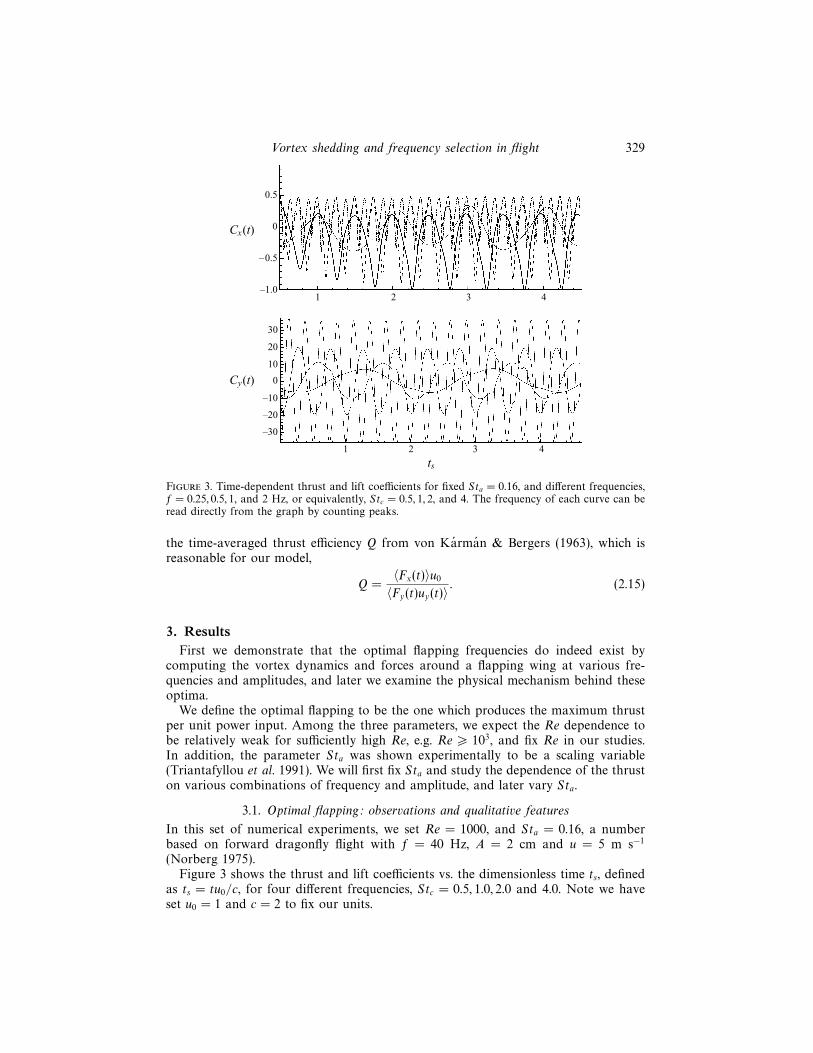
Figure 3. Time-dependent thrust and lift coefficients for fixed Sta = 0.16, and different frequencies,f = 0.25, 0.5, 1, and 2 Hz, or equivalently, Stc = 0.5, 1, 2, and 4. The frequency of each curve can beread directly from the graph by counting peaks.

the time-averaged thrust efficiency Q from von Karman & Bergers (1963), which isreasonable for our model,

Q =〈Fx(t)〉u0

〈Fy(t)uy(t)〉. (2.15)

3. Results

First we demonstrate that the optimal flapping frequencies do indeed exist bycomputing the vortex dynamics and forces around a flapping wing at various fre-quencies and amplitudes, and later we examine the physical mechanism behind theseoptima.

We define the optimal flapping to be the one which produces the maximum thrustper unit power input. Among the three parameters, we expect the Re dependence tobe relatively weak for sufficiently high Re, e.g. Re > 103, and fix Re in our studies.In addition, the parameter Sta was shown experimentally to be a scaling variable(Triantafyllou et al. 1991). We will first fix Sta and study the dependence of the thruston various combinations of frequency and amplitude, and later vary Sta.

3.1. Optimal flapping: observations and qualitative features

In this set of numerical experiments, we set Re = 1000, and Sta = 0.16, a numberbased on forward dragonfly flight with f = 40 Hz, A = 2 cm and u = 5 m s−1

(Norberg 1975).Figure 3 shows the thrust and lift coefficients vs. the dimensionless time ts, defined

as ts = tu0/c, for four different frequencies, Stc = 0.5, 1.0, 2.0 and 4.0. Note we haveset u0 = 1 and c = 2 to fix our units.

330 Z. J. Wang

Stc 4 2 1 0.5

〈Cx〉 0.18 −0.06 −0.24 −0.08〈Cxp〉 −0.02 −0.18 −0.27 −0.12〈Cxν〉 0.20 0.12 0.03 0.04Q(%) / 1.2 13.5 11.5

Table 1. Thrust coefficient 〈Cx〉 and its two contributions from the pressure force (Ctp) and theviscous force (Ctν) as a function of Stc. Efficiency is calculated only in the cases of positive thrust.The Reynolds number is 1000.

The lift coefficients Cy in the bottom plot vary symmetrically about the zero mean,thus the average vertical force is zero as expected from the symmetric flapping. Littlebumps on the three low-frequency curves result from the dynamics of the leading-edgevortices as we shall see in the next figure.

On the other hand, the thrust coefficients Cx are asymmetric about the zero axis,because the fore-and-aft symmetry is broken by the mean forward velocity field. Thefrequency of Cx is twice that of Cy , because the thrust is generated in both the upand down strokes. By definition, a negative value of Cx corresponds to a thrust in themean forward direction. In table 1, we tabulate the average thrust coefficient and theefficiency Q. 〈Cx〉 and Q reach maxima at Stc ∼ 1.

Next we examine the qualitative features of the associated vortex dynamics in thesefour cases. First the vortices in the wake rotate in the opposite direction comparedto a von Karman wake. Hence the induced flow has a component moving backwardwith respect to the wing to generate a thrust (von Karman & Bergers 1963). As aside remark, the apparent downward drift in both the experiments and these picturesis a transient behaviour due to the initial condition. We check this by repeating thesame computation with the initial flap reversed; the small drift is also reversed.

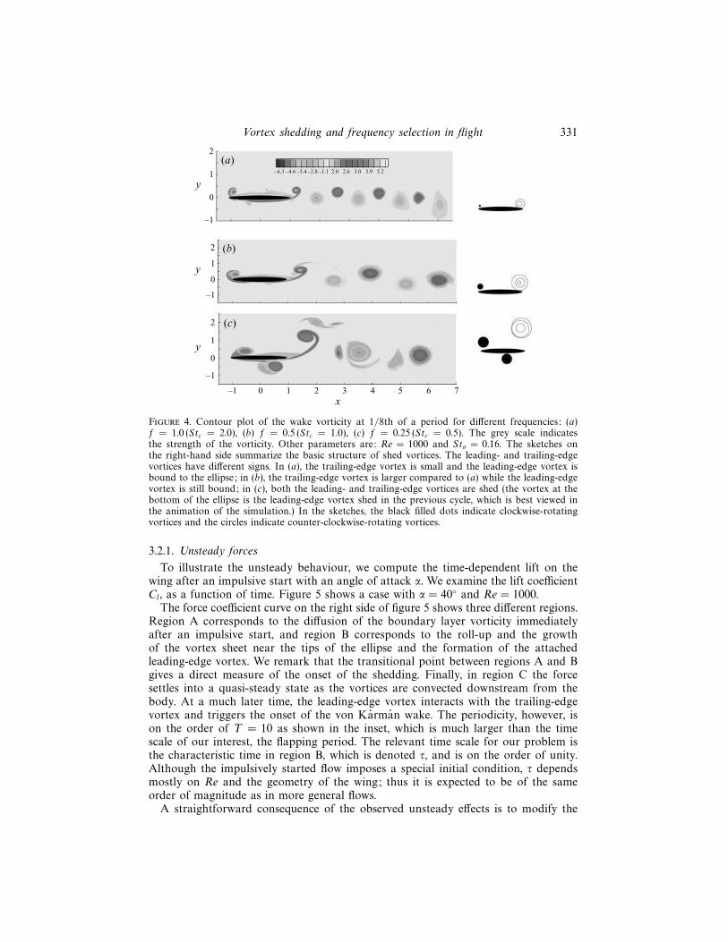
During each period, the trailing-edge vortex begins to shed and grow at the turn ofa flap, but the shedding of the leading-edge vortex depends on the angle of attack andthe flapping frequency. In figure 4, we compare the vorticity contours for differentflapping frequencies at 1/8th of a period. We sketch the basic vortex features nextto these figures. In the case of the highest Stc, the trailing-edge vortex is relativelysmall, as are the net circulation around the wing and the forces. As Stc decreases, thetrailing-edge vortex grows and the forces increase. Finally, as Stc further increases,the leading-edge vortex, which has the opposite sign to the trailing-edge vortex startsto shed and reduce the net circulation and the forces. The middle value of Stccorresponds to the observed optimal thrust and efficiency. To understand these vortexdynamics more quantitatively, we next analyse the growth of vortices and forces in asingle stroke.

3.2. Single-stroke dynamics

The previous pictures suggest that the following two processes may play significantroles: (1) the unsteady forces due to the trailing-edge vortex growth, similar to theWagner effect (Wagner 1921), and (2) the shedding of the leading-edge vortex asa function of Stc. We now investigate these effects in a single stroke moving withvelocity U at an angle of attack α, which serves as a snapshot of a flapping wing, withU the sum of u0 and u1, α = tan−1[u1(t)/u0]. The lift is defined to be orthogonal to U,and its forward component corresponds to the instantaneous thrust in the flappingmodel.

Vortex shedding and frequency selection in flight 331

2

–1

y

2

0y

2

0

y

–1 0 1 2 3 4 5 6 7

–1

1

0

1

1

–1

x

(a)

(b)

(c)

5.23.93.02.62.0–1.1–2.8–3.4–4.6–6.3

Figure 4. Contour plot of the wake vorticity at 1/8th of a period for different frequencies: (a)f = 1.0 (Stc = 2.0), (b) f = 0.5 (Stc = 1.0), (c) f = 0.25 (Stc = 0.5). The grey scale indicatesthe strength of the vorticity. Other parameters are: Re = 1000 and Sta = 0.16. The sketches onthe right-hand side summarize the basic structure of shed vortices. The leading- and trailing-edgevortices have different signs. In (a), the trailing-edge vortex is small and the leading-edge vortex isbound to the ellipse; in (b), the trailing-edge vortex is larger compared to (a) while the leading-edgevortex is still bound; in (c), both the leading- and trailing-edge vortices are shed (the vortex at thebottom of the ellipse is the leading-edge vortex shed in the previous cycle, which is best viewed inthe animation of the simulation.) In the sketches, the black filled dots indicate clockwise-rotatingvortices and the circles indicate counter-clockwise-rotating vortices.

3.2.1. Unsteady forces

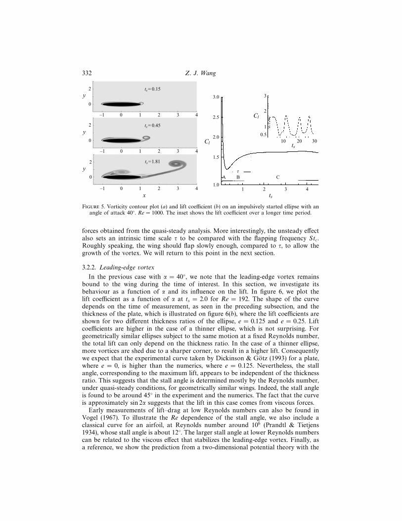
To illustrate the unsteady behaviour, we compute the time-dependent lift on thewing after an impulsive start with an angle of attack α. We examine the lift coefficientCl , as a function of time. Figure 5 shows a case with α = 40◦ and Re = 1000.

The force coefficient curve on the right side of figure 5 shows three different regions.Region A corresponds to the diffusion of the boundary layer vorticity immediatelyafter an impulsive start, and region B corresponds to the roll-up and the growthof the vortex sheet near the tips of the ellipse and the formation of the attachedleading-edge vortex. We remark that the transitional point between regions A and Bgives a direct measure of the onset of the shedding. Finally, in region C the forcesettles into a quasi-steady state as the vortices are convected downstream from thebody. At a much later time, the leading-edge vortex interacts with the trailing-edgevortex and triggers the onset of the von Karman wake. The periodicity, however, ison the order of T = 10 as shown in the inset, which is much larger than the timescale of our interest, the flapping period. The relevant time scale for our problem isthe characteristic time in region B, which is denoted τ, and is on the order of unity.Although the impulsively started flow imposes a special initial condition, τ dependsmostly on Re and the geometry of the wing; thus it is expected to be of the sameorder of magnitude as in more general flows.

A straightforward consequence of the observed unsteady effects is to modify the

332 Z. J. Wang

2

y

2

0

y

2

0

y

–1 0 1 2 3 4

0

x

–1 0 1 2 3 4

–1 0 1 2 3 4

ts = 0.45

ts =1.81

ts = 0.15

3.0

2.5

2.0

1.5

1.01 2 3 4

ts

Cl

s

A B C

2Cl

3

1

0.5

10 20 30ts

Figure 5. Vorticity contour plot (a) and lift coefficient (b) on an impulsively started ellipse with anangle of attack 40◦. Re = 1000. The inset shows the lift coefficient over a longer time period.

forces obtained from the quasi-steady analysis. More interestingly, the unsteady effectalso sets an intrinsic time scale τ to be compared with the flapping frequency Stc.Roughly speaking, the wing should flap slowly enough, compared to τ, to allow thegrowth of the vortex. We will return to this point in the next section.

3.2.2. Leading-edge vortex

In the previous case with α = 40◦, we note that the leading-edge vortex remainsbound to the wing during the time of interest. In this section, we investigate itsbehaviour as a function of α and its influence on the lift. In figure 6, we plot thelift coefficient as a function of α at ts = 2.0 for Re = 192. The shape of the curvedepends on the time of measurement, as seen in the preceding subsection, and thethickness of the plate, which is illustrated on figure 6(b), where the lift coefficients areshown for two different thickness ratios of the ellipse, e = 0.125 and e = 0.25. Liftcoefficients are higher in the case of a thinner ellipse, which is not surprising. Forgeometrically similar ellipses subject to the same motion at a fixed Reynolds number,the total lift can only depend on the thickness ratio. In the case of a thinner ellipse,more vortices are shed due to a sharper corner, to result in a higher lift. Consequentlywe expect that the experimental curve taken by Dickinson & Gotz (1993) for a plate,where e = 0, is higher than the numerics, where e = 0.125. Nevertheless, the stallangle, corresponding to the maximum lift, appears to be independent of the thicknessratio. This suggests that the stall angle is determined mostly by the Reynolds number,under quasi-steady conditions, for geometrically similar wings. Indeed, the stall angleis found to be around 45◦ in the experiment and the numerics. The fact that the curveis approximately sin 2α suggests that the lift in this case comes from viscous forces.

Early measurements of lift–drag at low Reynolds numbers can also be found inVogel (1967). To illustrate the Re dependence of the stall angle, we also include aclassical curve for an airfoil, at Reynolds number around 106 (Prandtl & Tietjens1934), whose stall angle is about 12◦. The larger stall angle at lower Reynolds numberscan be related to the viscous effect that stabilizes the leading-edge vortex. Finally, asa reference, we show the prediction from a two-dimensional potential theory with the

Vortex shedding and frequency selection in flight 333

2.5

2.0

1.5

1.0

0.5

0 10 20 30 40 50 60 70 80 90

Cl

(a)

p (1+e)sin(α)

Re =192 (numerics)Re >>106 (airfoil)2d theoryRe =192 (exp.)

0 10 20 30 40 50 60 70 80 90

α (deg.)

e = 0.125e = 0.25

2.5

2.0

1.5

1.0

0.5

Cl

(b)

Figure 6. (a) Lift coefficient as a function of angle of attack. The experimental curve is taken fromfigure 4 in Dickinson & Gotz (1993). The data are measured at ts = 2.0. The classical curve for anairfoil curve is from Prandtl and Tietjens (1934). (b) Lift coefficient as a function of the thicknessratio of the ellipse.

Kutta condition applied to the trailing edge approximated by the tip of the ellipse.Understandably, the classical theory fits the airfoil data with a horizontal shift, toaccount for the asymmetry, but not the lower Reynolds number flows.

The dynamics of the leading-edge vortex is directly connected to the forces on thewing. At Re ∼ 1000, the lift is dominated by the pressure, which can be expressed bythe vorticity flux as

P (θ) = ρν

∫ θ

0

∂ω

∂nds, (3.1)

where n is the normal vector at the surface, and ds is the line segment along the

334 Z. J. Wang

(a) (b)

100 200 300

–0.4

0

0.4

0.8

P

α = 4.5°

0y

1

2

–1

–1–2 0 1 2 3

100 200 300–1–2 0 1 2 3

100 200 300–1–2 0 1 2 3

–0.8

0.8

P

0

–1.6

–2

–0.8

0.8

P0

–1.6

–2

α = 42.5°

α = 72°

x h

0

y

2

3

1

0

y

2

3

1

Figure 7. Vorticity contours (a) and pressure distribution (b) around a wing for different angle ofattack α. θ = [0, 180◦] correspond to the upper surface, and θ = [180◦, 360◦] the lower surface.

ellipse, which is parameterized by θ. In figure 7 we show the pressure distributionfor three typical cases, α = 4.5◦, α = 42.5◦, and α = 72◦ at time t = 2.2. For eachcase, we also show the corresponding vorticity configuration. We note that in thecases of the smallest and largest α, both leading- and trailing-edge vortices are shed,while in the other case, the leading-edge vortex remains bound. The presence of thisleading-edge vortex induces a lower pressure region, seen as a dip in the pressure

Vortex shedding and frequency selection in flight 335

distribution, which enhances the lift. Although the three-dimensional leading-edgevortex is different, and has a strong component in the axial direction, as seen in therecent work by Ellington (1984), in an early work Savage, Newman & Wong (1978)applied the two-dimensional potential theory to flows around a plate with the presenceof a leading-edge vortex at an assumed position, and they found a substantial increaseof the force. Our computation can provide a further input to the two-dimensionaltheory with the position and strength of the leading-edge vortex, governed by theNavier–Stokes dynamics. This provides a basis for our future modelling of theseleading-edge vortices.

3.3. Optimal flapping: explanations

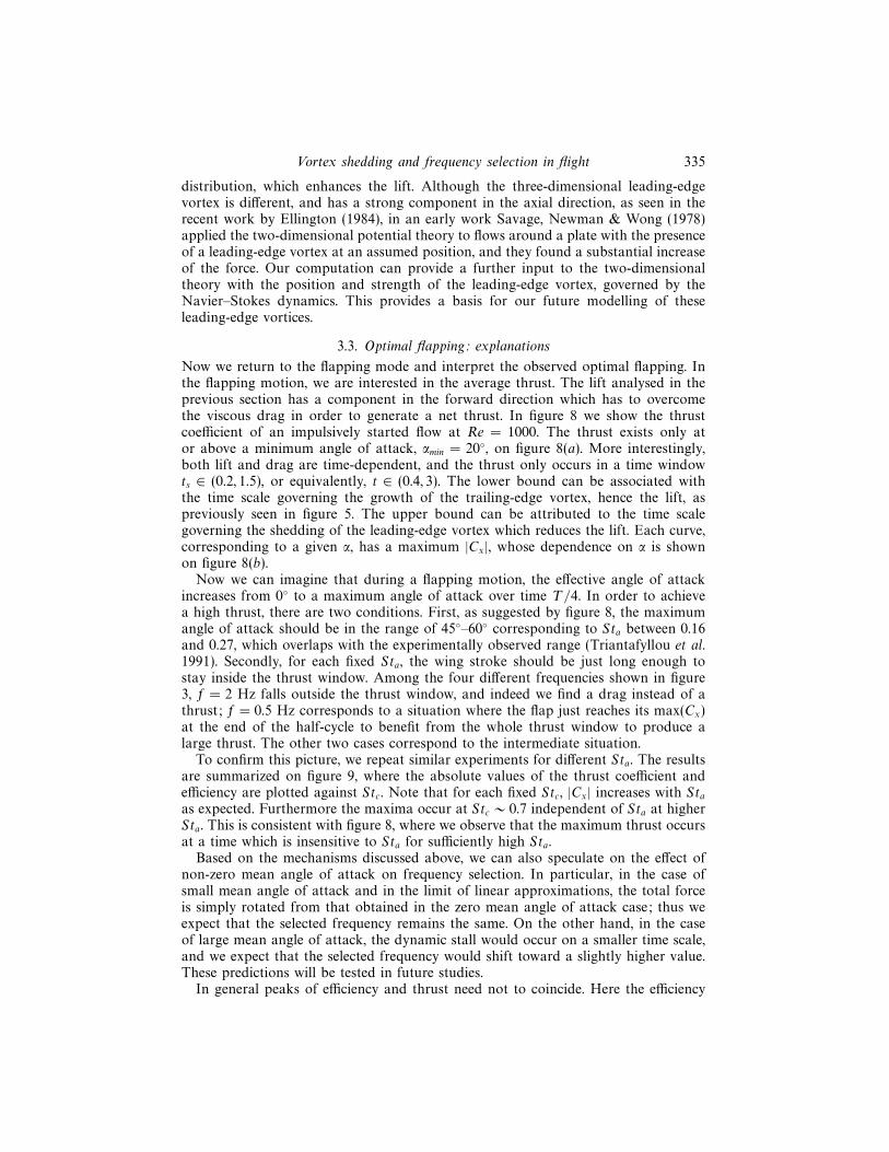
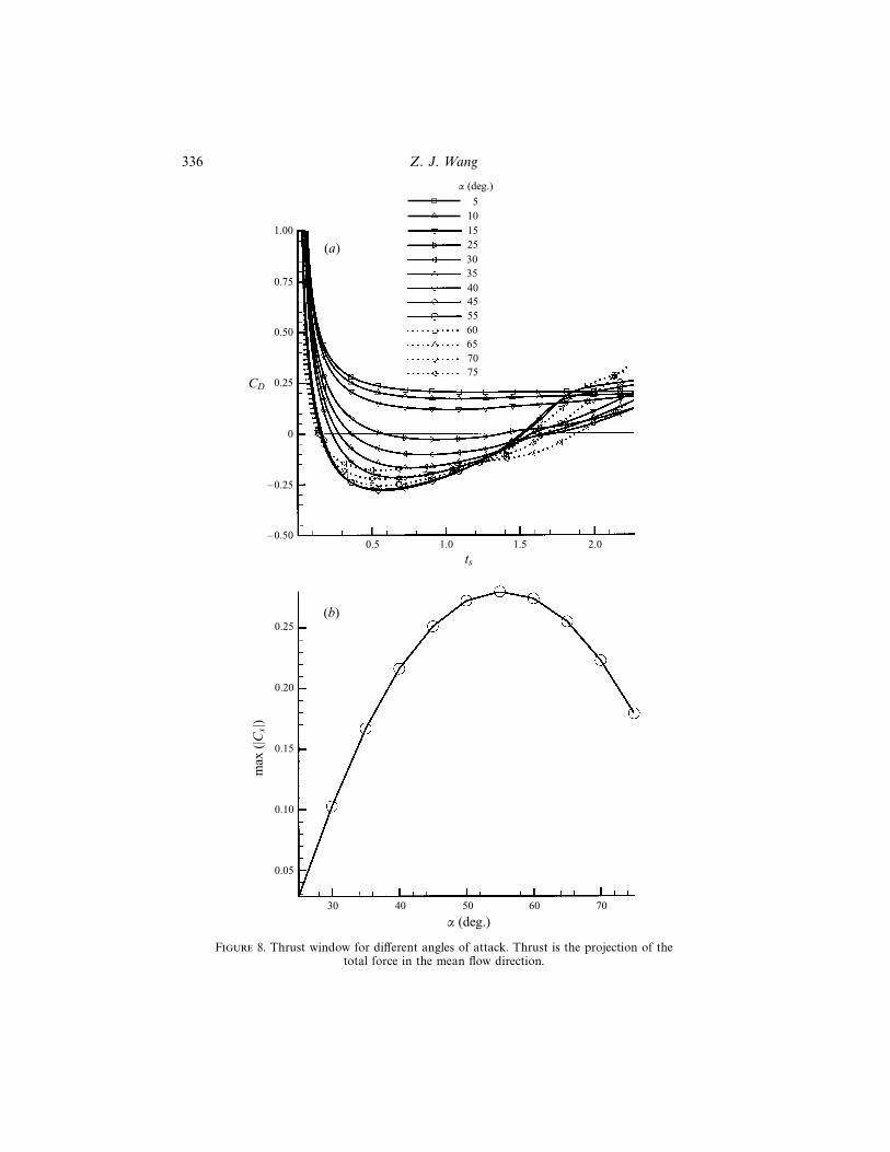
Now we return to the flapping mode and interpret the observed optimal flapping. Inthe flapping motion, we are interested in the average thrust. The lift analysed in theprevious section has a component in the forward direction which has to overcomethe viscous drag in order to generate a net thrust. In figure 8 we show the thrustcoefficient of an impulsively started flow at Re = 1000. The thrust exists only ator above a minimum angle of attack, αmin = 20◦, on figure 8(a). More interestingly,both lift and drag are time-dependent, and the thrust only occurs in a time windowts ∈ (0.2, 1.5), or equivalently, t ∈ (0.4, 3). The lower bound can be associated withthe time scale governing the growth of the trailing-edge vortex, hence the lift, aspreviously seen in figure 5. The upper bound can be attributed to the time scalegoverning the shedding of the leading-edge vortex which reduces the lift. Each curve,corresponding to a given α, has a maximum |Cx|, whose dependence on α is shownon figure 8(b).

Now we can imagine that during a flapping motion, the effective angle of attackincreases from 0◦ to a maximum angle of attack over time T/4. In order to achievea high thrust, there are two conditions. First, as suggested by figure 8, the maximumangle of attack should be in the range of 45◦–60◦ corresponding to Sta between 0.16and 0.27, which overlaps with the experimentally observed range (Triantafyllou et al.1991). Secondly, for each fixed Sta, the wing stroke should be just long enough tostay inside the thrust window. Among the four different frequencies shown in figure3, f = 2 Hz falls outside the thrust window, and indeed we find a drag instead of athrust; f = 0.5 Hz corresponds to a situation where the flap just reaches its max(Cx)at the end of the half-cycle to benefit from the whole thrust window to produce alarge thrust. The other two cases correspond to the intermediate situation.

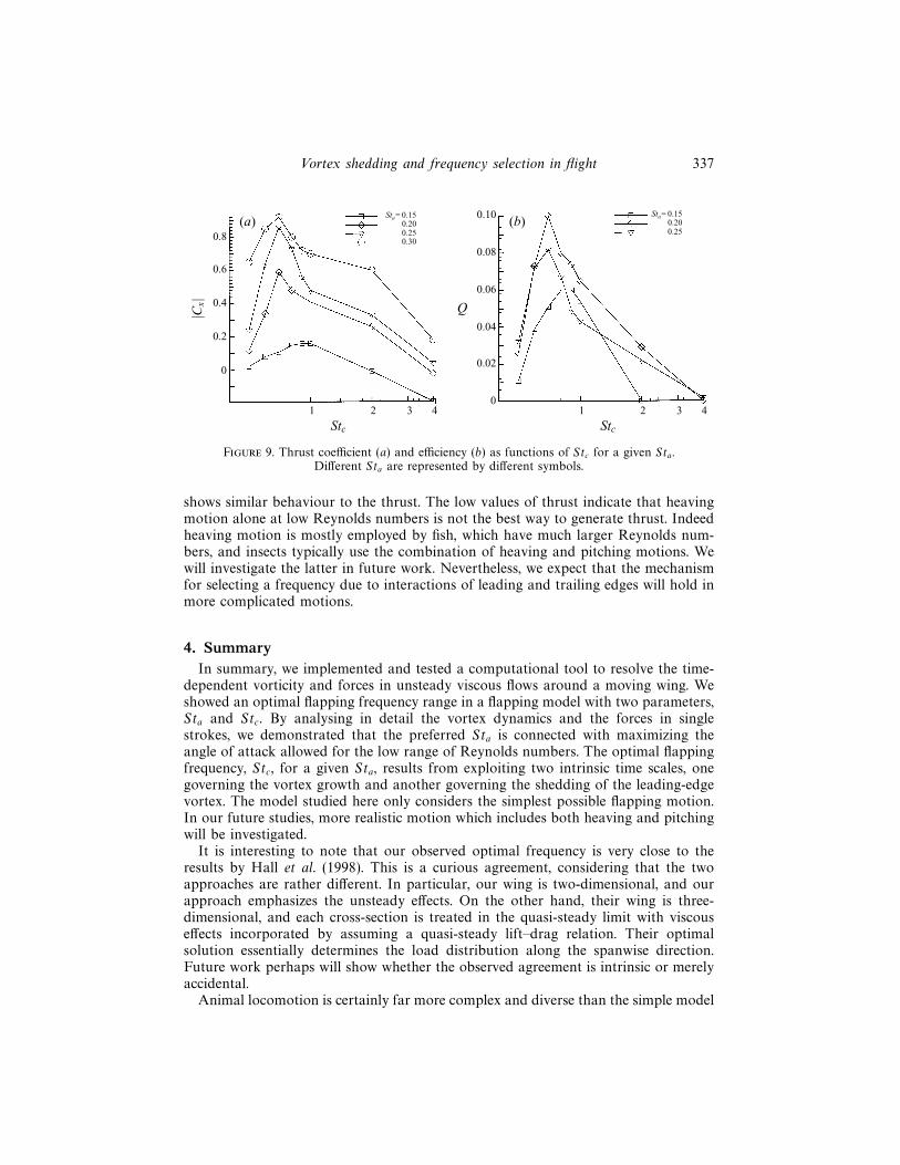
To confirm this picture, we repeat similar experiments for different Sta. The resultsare summarized on figure 9, where the absolute values of the thrust coefficient andefficiency are plotted against Stc. Note that for each fixed Stc, |Cx| increases with Staas expected. Furthermore the maxima occur at Stc ∼ 0.7 independent of Sta at higherSta. This is consistent with figure 8, where we observe that the maximum thrust occursat a time which is insensitive to Sta for sufficiently high Sta.

Based on the mechanisms discussed above, we can also speculate on the effect ofnon-zero mean angle of attack on frequency selection. In particular, in the case ofsmall mean angle of attack and in the limit of linear approximations, the total forceis simply rotated from that obtained in the zero mean angle of attack case; thus weexpect that the selected frequency remains the same. On the other hand, in the caseof large mean angle of attack, the dynamic stall would occur on a smaller time scale,and we expect that the selected frequency would shift toward a slightly higher value.These predictions will be tested in future studies.

In general peaks of efficiency and thrust need not to coincide. Here the efficiency

336 Z. J. Wang

(a)

(b)

1.00

0.75

0.50

0

0.25

–0.25

–0.500.5 1.0 1.5 2.0

ts

CD

5

10

15

25

30

45

55

35

40

60

75

65

70

α (deg.)

α (deg.)

30 40 50 60 70

0.05

0.10

0.15

0.20

0.25

max

(|C

x|)

Figure 8. Thrust window for different angles of attack. Thrust is the projection of thetotal force in the mean flow direction.

Vortex shedding and frequency selection in flight 337

(a)

|Cx|

0

0.2

0.4

0.6

0.8

1 2 3 4

Stc

1 2 3 4

Stc

0

0.02

0.04

0.06

0.08

0.10(b)

Q

Sta= 0.15Sta= 0.20Sta= 0.25Sta= 0.30

Sta= 0.15Sta= 0.20Sta= 0.25

Figure 9. Thrust coefficient (a) and efficiency (b) as functions of Stc for a given Sta.Different Sta are represented by different symbols.

shows similar behaviour to the thrust. The low values of thrust indicate that heavingmotion alone at low Reynolds numbers is not the best way to generate thrust. Indeedheaving motion is mostly employed by fish, which have much larger Reynolds num-bers, and insects typically use the combination of heaving and pitching motions. Wewill investigate the latter in future work. Nevertheless, we expect that the mechanismfor selecting a frequency due to interactions of leading and trailing edges will hold inmore complicated motions.

4. Summary

In summary, we implemented and tested a computational tool to resolve the time-dependent vorticity and forces in unsteady viscous flows around a moving wing. Weshowed an optimal flapping frequency range in a flapping model with two parameters,Sta and Stc. By analysing in detail the vortex dynamics and the forces in singlestrokes, we demonstrated that the preferred Sta is connected with maximizing theangle of attack allowed for the low range of Reynolds numbers. The optimal flappingfrequency, Stc, for a given Sta, results from exploiting two intrinsic time scales, onegoverning the vortex growth and another governing the shedding of the leading-edgevortex. The model studied here only considers the simplest possible flapping motion.In our future studies, more realistic motion which includes both heaving and pitchingwill be investigated.

It is interesting to note that our observed optimal frequency is very close to theresults by Hall et al. (1998). This is a curious agreement, considering that the twoapproaches are rather different. In particular, our wing is two-dimensional, and ourapproach emphasizes the unsteady effects. On the other hand, their wing is three-dimensional, and each cross-section is treated in the quasi-steady limit with viscouseffects incorporated by assuming a quasi-steady lift–drag relation. Their optimalsolution essentially determines the load distribution along the spanwise direction.Future work perhaps will show whether the observed agreement is intrinsic or merelyaccidental.

Animal locomotion is certainly far more complex and diverse than the simple model

338 Z. J. Wang

considered here. Therefore it is difficult to compare directly the exact numerical valuesof the observed optimal frequencies with the biological data. Nevertheless, the scalingresult shown in figure 9, i.e. Stc ∼ 0.7, suggests that the optimal frequencies areinversely proportional to the dimension of the wing. This is consistent with the datacompiled by Greenewalt (1962) in his figures 10 and 12 for birds and insect flight,covering scales of almost three decades, despite the scatter in the data. This apparentagreement does at least encourage one to ask whether the unsteady aerodynamicsmight guide the selection of frequency in animal flight.

Finally we remark that independent of their possible implications in biologicalflight, these observed optimal frequencies should be directly of interest to the designof mechanical flapping wings, especially in the light of recent research efforts in microair vehicles (MAV).

I am grateful to Steve Childress and Mike Shelley for advice and useful discussions,Jianguo Liu for the ec4 code for cavity flows, David Muraki, and John Wettlaufer forcritiques of the manuscript. Finally I thank NERSC for providing the supercomputerCPU time. The work is supported by NSF grant No. DMS-9400912 and DMS-9510356 and DOE grant No. DE-FG02-88ER25053.

Appendix. Testing the code with impulsively started flows past a cylinder

We test the code in three ways for flow past an impulsively started cylinder. Firstwe find a simple example where the approximate solution to the Navier–Stokesequation is known. Secondly, we compare the computed unsteady velocity field withwell-documented experiments by Bouard & Coutanceau (1980). Finally we computethe flow with different resolutions to study its convergence property.

As a first test, we note that after an impulsive start, due to the no-slip boundarycondition a thin boundary layer builds up at the surface of the cylinder and diffusesout radially as time increases. The flow outside the boundary layer, however, can stillbe adequately described by the potential flow:

Ψ = −u0

(

r − a2

r

)

sin θ, (A 1)

u(r) = u0

(

1 − a2

r2

)

cos θ, (A 2)

uθ(r) = −u0

(

1 +a2

r2

)

sin θ, (A 3)

where u0 is the velocity of the cylinder and a the radius. We compute at Re = 100with a resolution 128 × 128. In figure 10, we plot the azimuthal velocity uθ(r) atT = 0.1 as a function of r/a with fixed θ = π/2. The numerical result agrees wellwith the potential solution outside the boundary layer.

To test the dynamics in the vortex wake, we followed the set up of Bouard &Coutanceau (1980) and computed the velocity field in the wake along the symmetryaxis. We compare the time dependent velocity field with the experiments in thecase of Re = 550. The computational grid is 128 × 128. In figure 10 we copied theexperimental points from figure 18 in Bouard & Coutanceau (1980) and overlaidour numerics on top of that. The agreement is remarkably good, considering thatthe numerics is strictly two-dimensional while the experiment is approximately two-dimensional, and the initial conditions are not exactly the same. In addition, we found

Vortex shedding and frequency selection in flight 339

2.00

1.75

1.50

1.25

1.00

1 2 3 4 5 6 7 8 9 10

r/a

(a)

(b)

numerics-1

theory

uh(r)

1.0

0.5

0

–0.5

–1.0

0.5 1 1.5 2.0 2.5

x/D

u

Figure 10. (a) Numerical result for azimuthal velocity uθ(r) vs. r compared with theory. (b) Velocity(u) at different locations along the symmetric axis (x/D) in the wake, where D is the diameterof the cylinder. Different symbols correspond to time of measurement (rescaled by D/u0) with anincrement of 0.5, starting from ts = 0.5 (solid circle). Lines are from the numerics, and points arefrom experiments (Bouard & Coutanceau 1980).

the separation angle at Re = 40 to be 52.6◦, which is close to the experimental value,53.4◦ (Coutanceau & Bouard 1977).

To further test the convergence of our code, we tested with three different resolu-tions: 64 × 64, 128 × 128, and 256 × 256. The time step is fixed to be dt = 10−4. Thissmall time step is due to the over-resolution in the case of 256×256. We ran the code

340 Z. J. Wang

for 100 steps, and examined the vorticity along the boundary of the cylinder at theco-located points. In particular, we expected that the ratios (ω64 − ω32)/(ω128 − ω64)converge to 2p for the pth-order method. We found the numerical ratios to be between16 to 20 along the boundary, consistent with our fourth-order discretization scheme.The convergence study for flow past an ellipse at Re = 10000 was also done in Wang,Liu & Childress (1999).

REFERENCES

Bouard, R. & Coutanceau, M. 1980 The early stage of development of the wake behind animpulsively started cylinder for 40 < Re < 104. J. Fluid Mech. 101, 583.

Childress, S. 1981 Mechanics of Swimming and Flying. Cambridge University Press.

Chopra, M. G. 1976 Large amplitude lunate-tail theory of fish locomotion. J. Fluid Mech. 74, 161.

Coutanceau, M. & Bouard, R. 1977 Experimental determination of the main features of theviscous flow in the wake of a circular cylinder in uniform translation. Part 1. Steady flow. J.Fluid Mech. 79, 231.

Dickinson, M. H. & Gotz, K. G. 1993 Unsteady aerodynamic performance of model wings at lowReynolds numbers. J. Exp. Biol. 174, 45.

Dickinson, M. H., Lehmann, F. O. & Sane, S. P. 1999 Wing rotation and the aerodynamic basis ofinsect flight. Science 284, 1954.

Dudley, R. & Ellington, C. P. 1990 Mechanics of forward flight in bumblebees II. Quasi-steadylift and power requirements. J. Exp. Biol. 148, 53.

E, W. & Liu, J.-G. 1996 Essentially compact schemes for unsteady viscous incompressible flows. J.Comput. Phys. 126, 122.

Ellington, C. P. 1984 The aerodynamics of hovering insect flight. Phil. Trans. R. Soc. Lond. B305, 1.

Ellington, C. P., Berg, C. van den, Willmott, A. P. & Thomas, A. L. R. 1996 Leading-edgevortices in insect flight. Nature 384, 626.

Freymuth, P., Gustafson, K. E. & Leben, R. 1992 Visualization and computation of hoveringmode. In Vortex Method and Vortex Motion (ed. K. Gustafson & J. Sethian), p. 143. SIAM,Philadelphia.

Glauert, H. 1929 The force and moment on an oscillating aerofoil. Tech. Rep. Aero. Res. Comm.1242, 742.

Gopalkrishnan, R., Triantafyllou, M. S. & Triantafyllou, G. S. 1998 Oscillating foils of highpropulsive efficiency J. Fluid Mech. 360, 41.

Gustafson, K. E. & Leben, R. 1991 Computation of dragonfly aerodynamics. Comput. Phys.Commun. 65, 121.

Greenewalt, C. H. 1962 Dimensional Relationships for Flying Animals, vol. 144, no 2, SmithsonianMiscellaneous Collections, Washington DC.

Gursul, I. & Ho, C.-M. 1992 Oscillating foils of high propulsive efficiency. AIAA J. 30, 1117.

Hall, K. C., Pigott, S. A. & Hall, S. R. 1998 Power requirements for large-amplitude flappingflight. J. Aircraft 35, 352.

Karman von, F. & Burgers, J. M. 1963 General aerodynamic theory – perfect fluids. In AerodynamicTheory (ed. W. Durand), vol. 2, Div. E. Springer.

Lighthill, M. J. 1970 Aquatic animal propulsion of high hydromechanical efficiency. J. Fluid Mech.44, 265.

Lighthill, M. J. 1975 Mathematical Biofluiddynamics. SIAM, Philadelphia.

Lighthill, M. J. 1977 Introduction to the scaling of aerial locomotion. In Scaling Effects in AnimalLocomotion (ed. T. Pedley), p. 365. Academic.

Liu, H., Ellington, C. P., Kawachi, K., Berg, C. van den & Willmott, A. P. 1998 A computationalfluid dynamics study of hawkmoth hovering. J. Exp. Biol. 201, 461.

Liu, H. & Kawachi, K. 1998 A numerical study of insect flight J. Comput. Phys. 146, 124.

Maxworthy, T. 1981 The fluid dynamics of insect flight. Ann. Rev. Fluid Mech. 13, 329.

Norberg, R. A. 1975 Hovering flight of the dragonfly Aeschna juncea L., kinematics and dynamics.

Vortex shedding and frequency selection in flight 341

In Swimming and Flying in Nature (ed. T. Y. Wu, C. J. Brokaw & C. Brennen), vol. 2, p. 763.Plenum.

Osborne, M. F. M. 1951 Aerodynamics of flapping flight with application to insects. J. Expl Biol.47, 561.

Pennycuick, C. J. 1968 On flapping motion of pigeons. J. Expl Biol. 49, 527.Phlips, P. J., East, R. A. & Pratt, N. H. 1981 An unsteady lifting line theory of flapping wings

with application to the forward flight of birds. J. Fluid Mech. 112, 321.Prandtl, L. & Tietjens, O. G. 1934 Applied Hydro- and Aeromechanics. McGraw-Hill.Savage, S., Newman, B. G. & Wong, D. T.-M. 1979 The role of vortices and unsteady effects during

the hovering flight of dragonflies. J. Expl Biol. 83, 59.Smith, M. J. C., Wilkin, P. J. & Williams, M. H. 1996 The advances of an unsteady method in

modeling the aerodynamic forces on rigid flapping wings. J. Expl Biol. 199, 1073.Somps, C. & Luttges, M. W. 1985 Dragonfly flight: Novel uses of unsteady separated flows. Science

228, 1326.Spedding, G. R. 1992 The aerodynamics of flight. In Mechanics of Animal Locomotion (ed.

R. M. Alexander), p. 51. Springer.Spedding, G. R. 1993 On the significance of unsteady effects in the aerodynamic performance of

flying animals. Contemp. Maths 141, 401.Triantafyllou, M. S., Triantafyllou, G. S. & Gopalkrishnan, R. 1991 Wake mechanics for

thrust generation in oscillation foils. Phys. Fluids A 3, 12.Tritton, D. J. 1992 Physical Fluid Dynamics. Oxford.Vogel, S. 1967 Flight in drosophila III. Aerodynamic characteristics of fly wings. J. Expl Biol. 46,

431.Wagner, H. 1921 Uber die Entstehung des dynamischen Auftriebes von Tragflueln. Z. Angew.

Math. Mech. 5, 17.Wakeling, J. M. & Ellington, C. P. 1997 Dragonfly flight II. Velocities, accelerations and kine-

matics of flapping flight. J. Expl Biol. 200, 557.Wang, Z. J. 1999 Efficient implementation of the exact far field boundary condition for Poisson

equation. J. Comput. Phys. 153, 666.Wang, Z. J., Liu, J.-G., & Childress, S. 1999 Corner vortex and secondary vortices in flow past an

ellipse. Phys. Fluids 11, 9.Weis-Fogh, T. & Jensen, M. 1956 Biology and physics of locust flight. Proc. R. Soc. B. 239, 415–585.Weis-Fogh, T. 1977 Dimensional analysis of hovering flight. In Scaling Effects in Animal Locomation

(ed. T. Pedley), p. 405. Academic.Wu, T. Y. 1977 Introduction to the scaling of aquatic animal locomotion. In Scaling Effects in

Animal Locomation (ed. T. Pedley), pp. 203–232. Academic.