vps 2008 educ example 1

Insert the front cover image in this header, then position and resize it !

EDUCATION PACKAGE

Tutorial Exercise 1

End Loaded Cantilever and Shell Element Studies

VIRTUAL PERFORMANCE SOLUTION 2008 EDUCATION PACKAGE © 2008 ESI Group Tutorial Exercise 1

page 2 of 28 GR/VPS_/09/01/00/A

EExxeerrcciissee 11

EEnndd LLooaaddeedd CCaannttiilleevveerr aanndd

SShheellll EElleemmeenntt

SSttuuddiieess

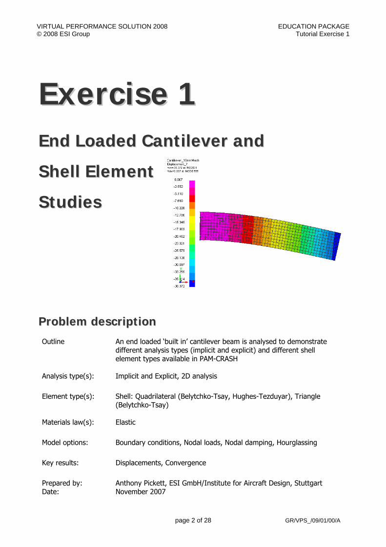
PPrroobblleemm ddeessccrriippttiioonn Outline An end loaded ‘built in’ cantilever beam is analysed to demonstrate

different analysis types (implicit and explicit) and different shell element types available in PAM-CRASH

Analysis type(s): Implicit and Explicit, 2D analysis

Element type(s): Shell: Quadrilateral (Belytchko-Tsay, Hughes-Tezduyar), Triangle (Belytchko-Tsay)

Materials law(s): Elastic

Model options: Boundary conditions, Nodal loads, Nodal damping, Hourglassing

Key results: Displacements, Convergence

Prepared by: Date:

Anthony Pickett, ESI GmbH/Institute for Aircraft Design, Stuttgart November 2007


page 3 of 28 GR/VPS_/09/01/00/A

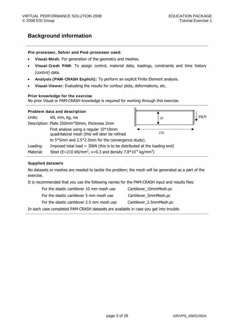
50

250

Background information

Pre-processor, Solver and Post-processor used:

• Visual-Mesh: For generation of the geometry and meshes.

• Visual-Crash PAM: To assign control, material data, loadings, constraints and time history

(control) data.

• Analysis (PAM-CRASH Explicit): To perform an explicit Finite Element analysis.

• Visual-Viewer: Evaluating the results for contour plots, deformations, etc. Prior knowledge for the exercise No prior Visual or PAM-CRASH knowledge is required for working through this exercise.

Problem data and description Units: kN, mm, kg, ms Description: Plate 250mm*50mm, thickness 2mm First analyse using a regular 10*10mm

quadrilateral mesh (this will later be refined to 5*5mm and 2.5*2.5mm for the convergence study). Loading: Imposed total load = 30kN (this is to be distributed at the loading end) Material: Steel (E=210 kN/mm2, ν=0.3 and density 7.8*10-6 kg/mm3)

Supplied datasets

No datasets or meshes are needed to tackle the problem; the mesh will be generated as a part of the exercise.

It is recommended that you use the following names for the PAM-CRASH input and results files:

For the elastic cantilever 10 mm mesh use Cantilever_10mmMesh.pc

For the elastic cantilever 5 mm mesh use Cantilever_5mmMesh.pc

For the elastic cantilever 2.5 mm mesh use Cantilever_2.5mmMesh.pc

In each case completed PAM-CRASH datasets are available in case you get into trouble.

30kN


page 4 of 28 GR/VPS_/09/01/00/A

Part 1: Using VCP to make cantilever beam model

Preparing the mesh (Visual Mesh)

Start the Visual Crash PAM program (VCP) and select the Visual-Mesh option, then click Set Active and Launch.

The program (on windows) may be in the START list of programs in the sub-set OPEN VTOS.

Remark: This will activate the meshing module of the VCP program dedicated to generating finite element meshes.

Select File and option New then specify the model unit system:

• Set Source Units to mm, kg, ms • Set Target Units to mm, kg, ms • Click OK

This specifies the unit systems (kN, mm, kg, ms) and allows a conversion to an alternative (target) system to be made if needed; we use the same for both. Alternatively, an old or partially completed model could be read in for further working using File with option Old and specifying the name of the file.

Some general comments before starting

Most mesh generation programs either allow the mesh to be generated by construction information (points, lines, surfaces, volumes, etc.) or use surface and volume data from CAD packages such as IDEAS and CATIA.

We shall generate the mesh here using some simple construction features in Visual-Mesh. The usual procedure is:

• Specify key points in x,y,z coordinates. • Join these points with lines, arcs, circles, spline curves, etc. • Use these lines as a basis to construct surface (patches) for 2D elements, or volumes for 3D

elements. • Care has to be made during this process to make sure the generated mesh is appropriate to

the loads, boundary conditions, part and material groupings that must be specified later in the process. Some advanced planning is needed!

Note: Visual-Mesh follows similar steps to make the mesh, but some useful tools are available to help simplify and speed the process.


page 5 of 28 GR/VPS_/09/01/00/A

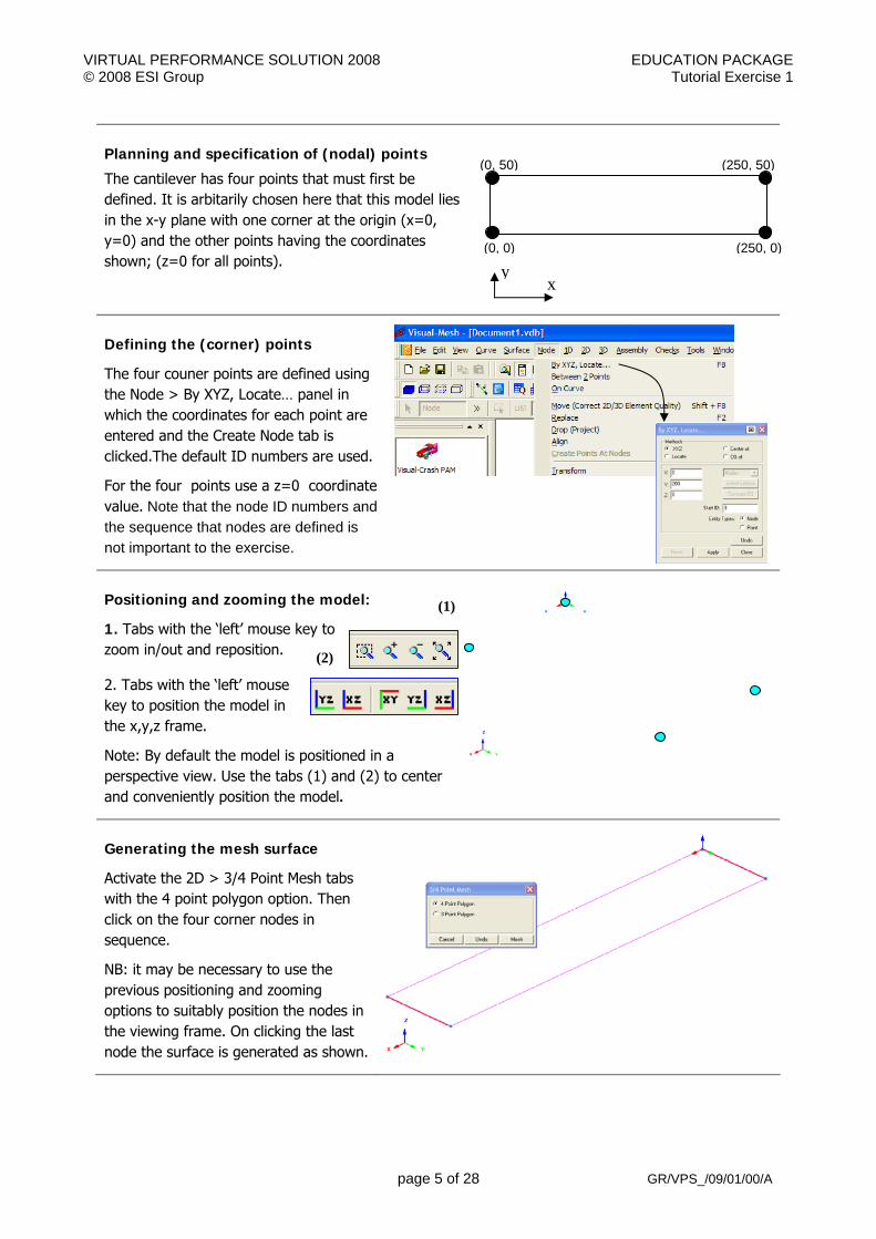
Planning and specification of (nodal) points

The cantilever has four points that must first be defined. It is arbitarily chosen here that this model lies in the x-y plane with one corner at the origin (x=0, y=0) and the other points having the coordinates shown; (z=0 for all points).

Defining the (corner) points

The four couner points are defined using the Node > By XYZ, Locate… panel in which the coordinates for each point are entered and the Create Node tab is clicked.The default ID numbers are used.

For the four points use a z=0 coordinate value. Note that the node ID numbers and the sequence that nodes are defined is not important to the exercise.

Positioning and zooming the model:

1. Tabs with the ‘left’ mouse key to zoom in/out and reposition.

2. Tabs with the ‘left’ mouse key to position the model in the x,y,z frame.

Note: By default the model is positioned in a perspective view. Use the tabs (1) and (2) to center and conveniently position the model.

Generating the mesh surface

Activate the 2D > 3/4 Point Mesh tabs with the 4 point polygon option. Then click on the four corner nodes in sequence.

NB: it may be necessary to use the previous positioning and zooming options to suitably position the nodes in the viewing frame. On clicking the last node the surface is generated as shown.

xy

(250, 0)

(250, 50)

(0, 0)

(1)

(0, 50)

(2)


page 6 of 28 GR/VPS_/09/01/00/A

Generating the mesh

Click on the Mesh tab and a new panel opens to control the mesh to be generated. Element sizes, grading of meshed and connection options (stitching) to possible adjacent meshes can be defined.

Use a 10mm element size and click the tab Create Mesh. The mesh will appear; accept this with the OK tab and click Close to close the mesh panel.

The last step is to remove “double nodes” : in Visual-mesh Check > Coincident Nodes. Press Check and Fuse all to merge double nodes

Ending the Visual-Mesh work

This now completes the meshing work with Visual Mesh. It is probably wise to save the data with File > Export to a suitable folder with a suitable name. Export this as a filename.pc file; which is the default name for a PAM-CRASH dataset.

E.g a suitable name could be Cantilever_10mmMesh.pc

Remark: It is possible to use the File > Save option to save data in a binary .vdb format, which could be useful for large models. However, PAM-CRASH only accepts the ASCII (.pc) format and so this is used as the basis to store data throughout these tutorial exercises.


page 7 of 28 GR/VPS_/09/01/00/A

Defining the model data (Visual-Crash PAM)

Preparation of the model(s) for analysis

This involves:

• Starting Visual Crash PAM for definition of entities (Loads, boundary conditions, etc.,)

• Application of boundary conditions (fixed restraints at the built-in end).

• Application of loading at the opposite end. • Definition of part (geometric) and material data. • Definition of the PAM-CRASH control data.

Starting the Visual-Crash PAM

1. It is probably wise with the training exercises to copy the mesh file just created to a new name and work with the copied file. If things go wrong it is possible to go back to the mesh file and start things again.

2. Copy Cantilever_10mmMesh.pc to Cantilever_10mmModel.pc.

3. Start the Visual-Crash PAM and read in the new file (Cantilever_10mmModel.pc) using FILE > Open.

Remark: For advanced users it is possible to activate Visual-Crash PAM directly in the Contex panel and perform meshing and entity definintion operation in one step, using the same dataset. It is probably not advisable for learning and so we shall separate the two steps.


page 8 of 28 GR/VPS_/09/01/00/A

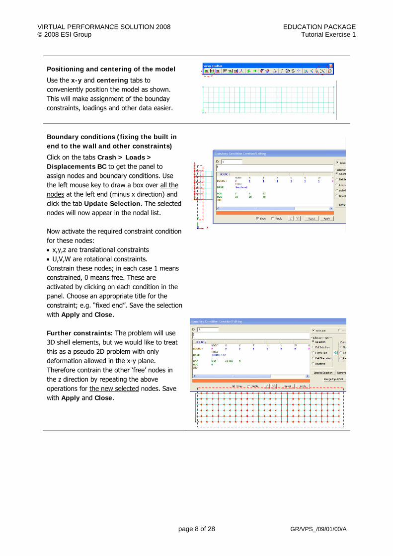
Positioning and centering of the model

Use the x-y and centering tabs to conveniently position the model as shown. This will make assignment of the bounday constraints, loadings and other data easier.

Boundary conditions (fixing the built in end to the wall and other constraints)

Click on the tabs Crash > Loads > Displacements BC to get the panel to assign nodes and boundary conditions. Use the left mouse key to draw a box over all the nodes at the left end (minus x direction) and click the tab Update Selection. The selected nodes will now appear in the nodal list. Now activate the required constraint condition for these nodes: • x,y,z are translational constraints • U,V,W are rotational constraints. Constrain these nodes; in each case 1 means constrained, 0 means free. These are activated by clicking on each condition in the panel. Choose an appropriate title for the constraint; e.g. “fixed end”. Save the selection with Apply and Close. Further constraints: The problem will use 3D shell elements, but we would like to treat this as a pseudo 2D problem with only deformation allowed in the x-y plane. Therefore contrain the other ‘free’ nodes in the z direction by repeating the above operations for the new selected nodes. Save with Apply and Close.


page 9 of 28 GR/VPS_/09/01/00/A

Loading conditions (at the opposite free end)

The aim now is to apply negative (y) loading at the free end. Click on the tabs Crash > Loads > Concentrated Loads to get the panel to assign nodal loads. Use the left mouse key to draw a box over all the nodes at the right end (plus x direction) and click the tab Update Selection. The selected nodes will now appear in the nodal list. Give the nodal loads a suitable title; e.g “load 5kN per node” so it can be easily identified in the PAM-CRASH dataset file. We now assign the loads to these nodes and the load direction. This is done using a load curve (which can have a constant value or a specific time history curve. 1. Click on LCUR and a new panel to define

the load curve will open. Click on NewCurve_1 and OK to define the data.

2. In the new panel define the load curve function. The x-axis is time and y-axis is applied load. Assume the load starts at zero and increases to a constant load of 5kN at 5 msecand is then held constant to the end simulation time for this problem (=10 msec to be defined later). Note that the applied loading is 5kN at each of the 6 nodes (=30kN total load at the free end).

3. Some final points: • The load so far defined is positive and we

would like this to be in the negative y-direction. A convenient way is to set the load scale factor SCALF =-1.

• Assign the load direction IDR=2 (= y direction)

• Make sure the load curve (LCUR=1) is assigned to this set of nodes.

Close and save the selection with Apply and Close.


page 10 of 28 GR/VPS_/09/01/00/A

Assigning the Material and Part data

This is done using two entities which are linked together; namely: 1. The Material data for material data such as

modulus, density and plasticity information. 2. The Part data for (geometric data such as

thickness).

1. Material data

Select Crash > Materials Editor and then select the type of Material Model; in this case use a 101 – ELASTIC_SHELL. Finally define the material data Steel (E=210 kN/mm2, ν=0.3 and density 7.8*10-6 kg/mm3). Save with Apply and Close. Remark: Make sure you use a consistent set of

units. Here kN, mm, msec and kg is used throughout; analysis results will also be in the same consistent units as the input.

2. Part data

This is easily done via the explorer panel: 1. First click on parts and the list of parts will open;

select the required part and the parts panel will open.

2. Set the shell thickness to 2mm. Click just below h and set this to 2 (=2mm).

3. Finally, the material to be linked to this part must be assigned. Click on IMAT and the materials panel will open. Select the required material and click OK.

Finish the part assignment with Apply and Close.

Output results

In order to study convergence it will be useful to have details of time history information for the corner node (A) and an element (eg B) at 50mm from the wall.

For the node click Crash > Output > Nodel TH and select the corner node (click on it with the left mouse key) Click on Update Selection; give a suitable title and finish with Close.

For the element repeat the process using Crash > Output > Element TH and selecting the required element.

B A


page 11 of 28 GR/VPS_/09/01/00/A

The PAM-CRASH control data must be set

This controls the analysis and allows specific data like the problem analysis time (in msecs in this case), specific output information and ouput intevals for the results to be defined.

• For example in the explorer panel, click on the Explorer > Pam Controls > Title and then open the title panel in edit mode by clicking the right mouse key or by clicking twice. A suitable title can now be added. This title will appear on all results plotted later using Visual Viewer and is important to help identify the analysis undertaken (e.g. Cantilever_10mmMesh). Save this information with Apply and Close.

• Similar steps are done for the RUNEND control (open, edit and enter 10.0 for the solution time).

• For the control OCTRL select the POINT option in THPOUTPUTwith 1000 which will save 1000 points of time history information for x-y graph outputs (to the .THP file); and the STATE option in DSYOUTPUT with 10 to give ten plots of the deformed structure (to the .DSYresults file). Save this information with Apply and Close.

Finally, special output options

By default only limited node and element time history information is stored on the .THP and .DSY files; for example, nodal displacements and velocities, and element local stresses. A wide range of additional information is available, but this must be specified. For example in the explore option Controls > Pam Controls > OCTRL click on the tab Advanced. Then click on SHLTHP > ALL > OK and click on SHLPLOT > ALL > OK to output all available shell contour variable to the .DSY and .THP files. Finish with Apply.

Saving the dataset (as a .pc file)

Export the model in the required directory with a suitable name; e.g. overwrite the now updated Cantilever_10mmModel.pc file. Click on File > Export and save the dataset. Be careful to make sure the directory location for the export is correct. Remark 1: Files save in this way have the PAM-CRASH input

file ASCII format and are readable. The File > Save option will save the model in a .vdb internal binary format.

Remark 2: Some other dataset formats (e.g. DYNA3D and NASTRAN) are also possible to be saved: See the Data type options.


page 12 of 28 GR/VPS_/09/01/00/A

The PAM-CRASH (filename.pc) data file

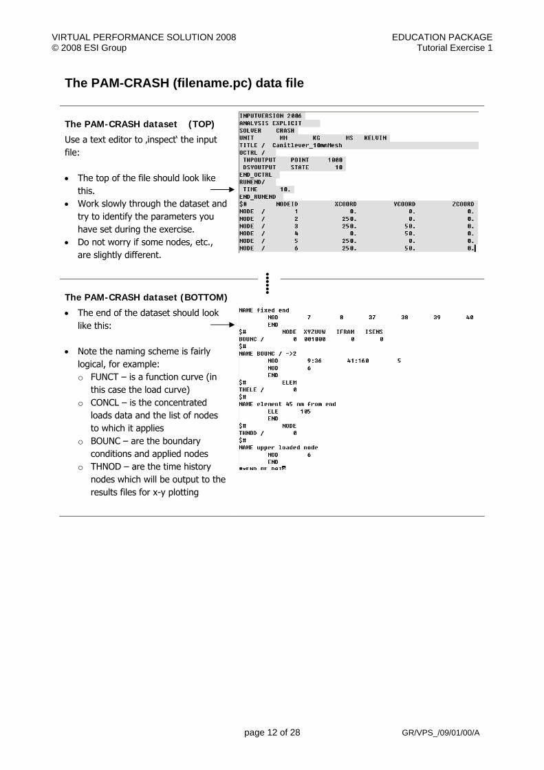
The PAM-CRASH dataset (TOP)

Use a text editor to ‚inspect‘ the input file: • The top of the file should look like

this. • Work slowly through the dataset and

try to identify the parameters you have set during the exercise.

• Do not worry if some nodes, etc., are slightly different.

The PAM-CRASH dataset (BOTTOM)

• The end of the dataset should look like this:

• Note the naming scheme is fairly

logical, for example: o FUNCT – is a function curve (in

this case the load curve) o CONCL – is the concentrated

loads data and the list of nodes to which it applies

o BOUNC – are the boundary conditions and applied nodes

o THNOD – are the time history nodes which will be output to the results files for x-y plotting

......


page 13 of 28 GR/VPS_/09/01/00/A

Part 2: Explicit analysis of the cantilever beam

Running a PAM-CRASH analysis

• Start the simulation run from the PAM-SYSTEM folder on the Desktop. The dataset file name and its location will be requested

• If the dataset is good it will proceed through the dataset initialisation phase into the solution phase

• If there are data errors the run will stop with an abnormal termination message. Inspect the output file for errors (search for ‘ERROR’ and investigate). Correct the dataset; preferably in VISUAL CRASH (or in the editor) and rerun the analysis


page 14 of 28 GR/VPS_/09/01/00/A

Evaluating the results (Visual Viewer) First, we shall look at selected results of the deformed structure and some information that are available for contour plots of the complete structure; these are stored in the .DSY file at selected time intevals (states). Following this we shall look at typical x-y plot information which is stored in the .THP file. The time intevals are different for both the .DSY and .THP output and were specified in the Visual Crash PAM session.

• filename.THP stores x-y time history plot information at selected points, elements, etc. • filename.DSY contains deformation and contour plots of the full structure.

Mesh plot results (.DSY file)

1. Start the Visual-Viewer program. First, you will see that the layout of the program and most options to visualise and manipulate the part are the same as those used in Visual-Mesh and Visual-Crash PAM.

2. Open the results files using File > Open. First open the DSY file (i.e. Cantilever_10mmModel.DSY) which contains deformed state and contour plot information for the complete structure. Alternatively, File > Open Project allows the files filename.DSY, filename.THP and filename.pc to be opened simultaneously-

3. Click Results > Animation Control and you will be able to visualise the model and use the adjacent panel to examine deformations, either at a certain time, or as a continuous animation.

Use the Speed Control option to change the viewing speed in the animation option.

Additional tabs are available for overlaying the Initial Mesh or Simultaneous Display for viewing selected states simultaneously. Click Close to exit this option.


page 15 of 28 GR/VPS_/09/01/00/A

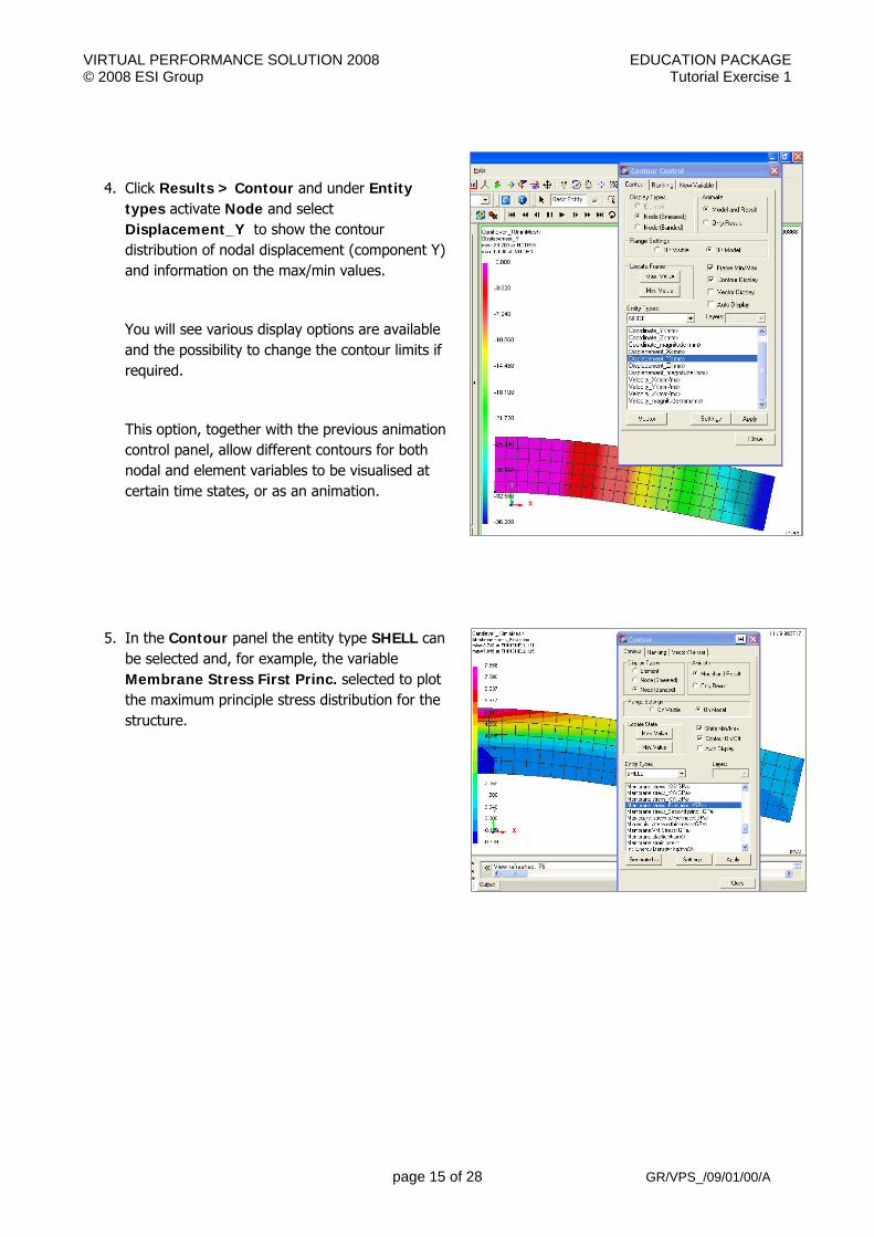
4. Click Results > Contour and under Entity types activate Node and select Displacement_Y to show the contour distribution of nodal displacement (component Y) and information on the max/min values.

You will see various display options are available and the possibility to change the contour limits if required.

This option, together with the previous animation control panel, allow different contours for both nodal and element variables to be visualised at certain time states, or as an animation.

5. In the Contour panel the entity type SHELL can be selected and, for example, the variable Membrane Stress First Princ. selected to plot the maximum principle stress distribution for the structure.


page 16 of 28 GR/VPS_/09/01/00/A

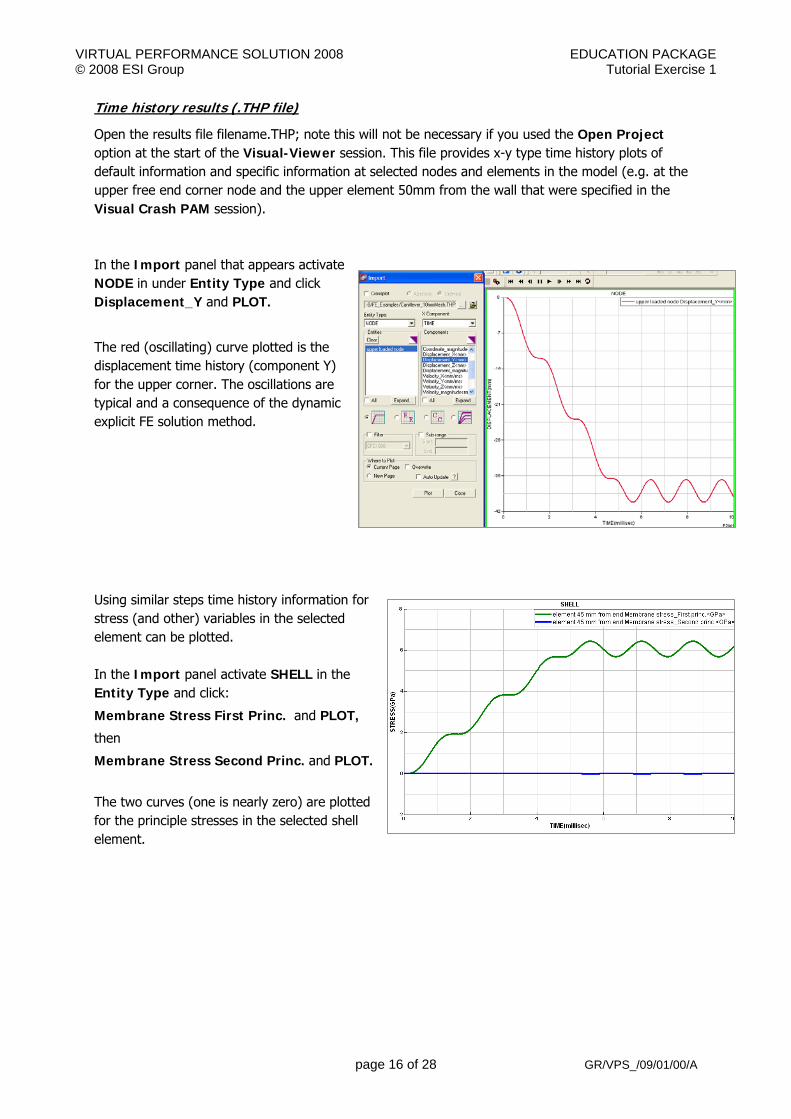
Time history results (.THP file)

Open the results file filename.THP; note this will not be necessary if you used the Open Project option at the start of the Visual-Viewer session. This file provides x-y type time history plots of default information and specific information at selected nodes and elements in the model (e.g. at the upper free end corner node and the upper element 50mm from the wall that were specified in the Visual Crash PAM session). In the Import panel that appears activate NODE in under Entity Type and click Displacement_Y and PLOT.

The red (oscillating) curve plotted is the displacement time history (component Y) for the upper corner. The oscillations are typical and a consequence of the dynamic explicit FE solution method.

Using similar steps time history information for stress (and other) variables in the selected element can be plotted. In the Import panel activate SHELL in the Entity Type and click:

Membrane Stress First Princ. and PLOT,

then

Membrane Stress Second Princ. and PLOT.

The two curves (one is nearly zero) are plotted for the principle stresses in the selected shell element.


page 17 of 28 GR/VPS_/09/01/00/A

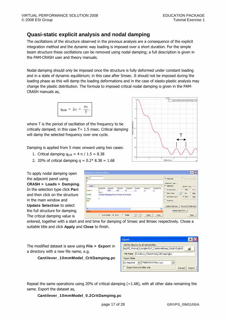
Quasi-static explicit analysis and nodal damping The oscillations of the structure observed in the previous analysis are a consequence of the explicit integration method and the dynamic way loading is imposed over a short duration. For the simple beam structure these oscillations can be removed using nodal damping; a full description is given in the PAM-CRASH user and theory manuals.

Nodal damping should only be imposed once the structure is fully deformed under constant loading and in a state of dynamic equilibrium; in this case after 5msec. It should not be imposed during the loading phase as this will damp the loading deformations and in the case of elasto-plastic analysis may change the plastic distribution. The formula to imposed critical nodal damping is given in the PAM-CRASH manuals as,

where T is the period of oscillation of the frequency to be critically damped; in this case T= 1.5 msec. Critical damping will damp the selected frequency over one cycle.

Damping is applied from 5 msec onward using two cases:

1. Critical damping qcrit = 4 π / 1.5 = 8.38

2. 20% of critical damping q = 0.2* 8.38 = 1.68

To apply nodal damping open the adjacent panel using CRASH > Loads > Damping. In the selection type click Part and then click on the structure in the main window and Update Selection to select the full structure for damping. The critical damping value is entered, together with a start and end time for damping of 5msec and 8msec respectively. Chose a suitable title and click Apply and Close to finish.

The modified dataset is save using File > Export in a directory with a new file name, e.g.

Cantilever_10mmModel_CritDamping.pc

Repeat the same operations using 20% of critical damping (=1.68), with all other data remaining the same. Export the dataset as,

Cantilever_10mmModel_0.2CritDamping.pc

T


page 18 of 28 GR/VPS_/09/01/00/A

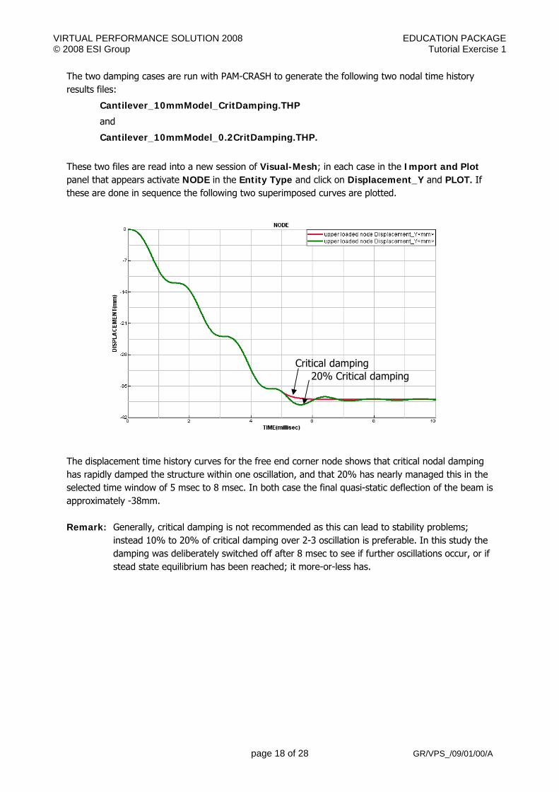
The two damping cases are run with PAM-CRASH to generate the following two nodal time history results files:

Cantilever_10mmModel_CritDamping.THP

and

Cantilever_10mmModel_0.2CritDamping.THP.

These two files are read into a new session of Visual-Mesh; in each case in the Import and Plot panel that appears activate NODE in the Entity Type and click on Displacement_Y and PLOT. If these are done in sequence the following two superimposed curves are plotted.

The displacement time history curves for the free end corner node shows that critical nodal damping has rapidly damped the structure within one oscillation, and that 20% has nearly managed this in the selected time window of 5 msec to 8 msec. In both case the final quasi-static deflection of the beam is approximately -38mm. Remark: Generally, critical damping is not recommended as this can lead to stability problems;

instead 10% to 20% of critical damping over 2-3 oscillation is preferable. In this study the damping was deliberately switched off after 8 msec to see if further oscillations occur, or if stead state equilibrium has been reached; it more-or-less has.

Critical damping20% Critical damping


page 19 of 28 GR/VPS_/09/01/00/A

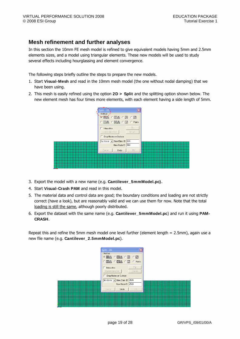
Mesh refinement and further analyses In this section the 10mm FE mesh model is refined to give equivalent models having 5mm and 2.5mm elements sizes, and a model using triangular elements. These new models will be used to study several effects including hourglassing and element convergence.

The following steps briefly outline the steps to prepare the new models.

1. Start Visual-Mesh and read in the 10mm mesh model (the one without nodal damping) that we have been using.

2. This mesh is easily refined using the option 2D > Split and the splitting option shown below. The new element mesh has four times more elements, with each element having a side length of 5mm.

3. Export the model with a new name (e.g. Cantilever_5mmModel.pc).

4. Start Visual-Crash PAM and read in this model.

5. The material data and control data are good; the boundary conditions and loading are not strictly correct (have a look), but are reasonably valid and we can use them for now. Note that the total loading is still the same, although poorly distributed.

6. Export the dataset with the same name (e.g. Cantilever_5mmModel.pc) and run it using PAM-CRASH.

Repeat this and refine the 5mm mesh model one level further (element length = 2.5mm), again use a new file name (e.g. Cantilever_2.5mmModel.pc).


page 20 of 28 GR/VPS_/09/01/00/A

The two refined analysis models are run with PAM-CRASH and are now compared with the already analysed 10mm mesh model. Only the undamped results are used in this comparison.

The three time history (.THP) result files for the 10mm, 5mm and 2.5mm mesh models are read into a new session of Visual-Viewer, in each case a plot of nodal Y-displacement for the free end corner node is plotted. The 10mm element gives the lowest average end displacement (-38mm), whereas the 5 mm and 2.5 mm element mesh models both show a have much greater average end displacements (-47mm).

A close inspection of the mesh at the restrained end, below, shows that the poorly distributed boundary conditions in the refined meshes has caused local hourglassing and led to (incorrect) greater end deflection. The boundary condition nodes come from the original 10mm meshed model, so only every second node in the 5mm mesh and every forth node in the 2.5mm meshed model is restrained. This is bad practice and all nodes should be restrained! However, it is an interesting result and the opportunity is taken in the next section to discuss hourglassing and methods to treat it.


page 21 of 28 GR/VPS_/09/01/00/A

Element types and hourglass control

Hourglassing is a problem of under-integration techniques used in the numerical integration of element stiffness, or other quantities, and is especially common in ‘one point’ integration elements used in explicit FE codes. Furthermore, it can is more easily excited in regular meshed structures. A full description of hourglass theory and its control is given in the PAM-CRASH theory manual.

Essentially, hourglass modes are certain element deformation modes that erroneously predict zero deformation energy at the element integration point, which is at the centre of the element. Three methods could be used here to eliminate, or limit its appearance:

1. Fully constrain all nodes at the boundary (the best and proper modelling approach), would stop the poor loading that has excited hourglassing in this case.

2. Use a different element type that does not have hourglass modes.

3. Apply different hourglass control, or increase the hourglass control parameters (this rarely is very effective).

The 5mm mesh model with 20% critical damping and the poor end restraints is used here to study some of these methods to stop hourglassing and correct prediction of end deflections.

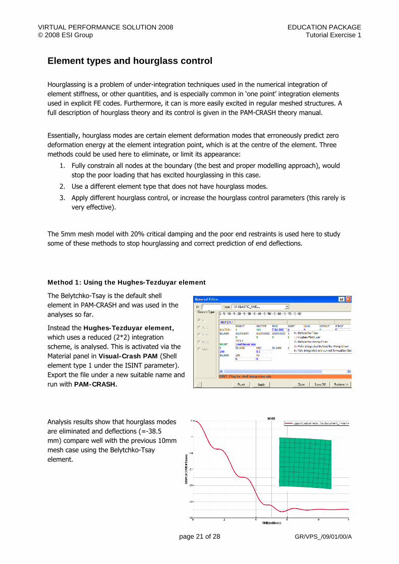
Method 1: Using the Hughes-Tezduyar element

The Belytchko-Tsay is the default shell element in PAM-CRASH and was used in the analyses so far.

Instead the Hughes-Tezduyar element, which uses a reduced (2*2) integration scheme, is analysed. This is activated via the Material panel in Visual-Crash PAM (Shell element type 1 under the ISINT parameter). Export the file under a new suitable name and run with PAM-CRASH.

Analysis results show that hourglass modes are eliminated and deflections (=-38.5 mm) compare well with the previous 10mm mesh case using the Belytchko-Tsay element.


page 22 of 28 GR/VPS_/09/01/00/A

Method 2: Using triangle elements

The Belytschko-Tsay element is used (parameter ISINT in the material cards) and the 5mm mesh model is modified to have triangle elements (note that there is a split option in Visual-Mesh to do this). Export the file under a new suitable name and run with PAM-CRASH. The maximum deflection is about -36mm.

Note in this case the poor boundary conditions have been used but there are no signs of hourglassing. Triangle elements do not have hourglass modes. Also, it can be seen that the end deflection is slightly less than the quadrilateral element mesh result; this is due to this element formulation being slightly stiffer.

Remark: Hourglassing is actually very rare in analyses and should not occur if the standard PAM-CRASH hourglass controls are used in under-integrated elements.


page 23 of 28 GR/VPS_/09/01/00/A

Element convergence (explicit analysis with the Hughes-Tezduyar element)

It is expected that a ‘well behaved’ finite element should show a convergence trend. That is, analysis with an increasingly refined mesh should tend toward a converged solution.

The following results compare maximum deflection for the 2.5mm, 5mm and 10mm mesh models using the fully integrated Hughes-Tezduyar element and 20% critical damping.

The element shows a good convergence trend and the final deflection can be expected to be about 40mm (for this element type).

10mm mesh (125 lements)

5mm mesh (500 lements)2.5mm mesh (2000 elements)

36

38,5

39,75

35,536

36,537

37,538

38,539

39,540

0 500 1000 1500 2000 2500

No. elements

End

defle

ctio

n


page 24 of 28 GR/VPS_/09/01/00/A

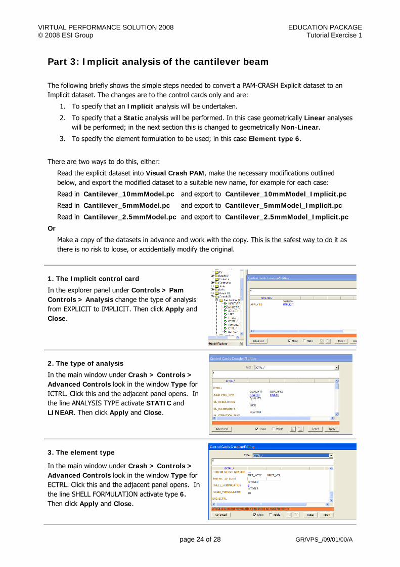
Part 3: Implicit analysis of the cantilever beam

The following briefly shows the simple steps needed to convert a PAM-CRASH Explicit dataset to an Implicit dataset. The changes are to the control cards only and are:

1. To specify that an Implicit analysis will be undertaken.

2. To specify that a Static analysis will be performed. In this case geometrically Linear analyses will be performed; in the next section this is changed to geometrically Non-Linear.

3. To specify the element formulation to be used; in this case Element type 6.

There are two ways to do this, either:

Read the explicit dataset into Visual Crash PAM, make the necessary modifications outlined below, and export the modified dataset to a suitable new name, for example for each case:

Read in Cantilever_10mmModel.pc and export to Cantilever_10mmModel_Implicit.pc

Read in Cantilever_5mmModel.pc and export to Cantilever_5mmModel_Implicit.pc

Read in Cantilever_2.5mmModel.pc and export to Cantilever_2.5mmModel_Implicit.pc

Or

Make a copy of the datasets in advance and work with the copy. This is the safest way to do it as there is no risk to loose, or accidentially modify the original.

1. The Implicit control card

In the explorer panel under Controls > Pam Controls > Analysis change the type of analysis from EXPLICIT to IMPLICIT. Then click Apply and Close.

2. The type of analysis

In the main window under Crash > Controls > Advanced Controls look in the window Type for ICTRL. Click this and the adjacent panel opens. In the line ANALYSIS TYPE activate STATIC and LINEAR. Then click Apply and Close.

3. The element type

In the main window under Crash > Controls > Advanced Controls look in the window Type for ECTRL. Click this and the adjacent panel opens. In the line SHELL FORMULATION activate type 6. Then click Apply and Close.


page 25 of 28 GR/VPS_/09/01/00/A

Static linear implicit results Use PAM-CRASH Implicit to run the three implicit cantilever beam problems; namely,

Cantilever_10mmModel_Implicit.pc Cantilever_5mmModel_Implicit.pc Cantilever_2.5mmModel_Implicit.pc

Results from the analysis are processed in exactly the same way as the previous explicit analyses using Visual Viewer; except that, in this case, only the initial and final deformed states are available and there is no .THP file. The following contour plots from the .DSY files show results of deformations for the three models.

The three implicit analyses show similar results to the explicit analyses with maximum y-deflections being:

for the 10mm mesh = 36.486 mm

for the 5mm mesh = 39.062 mm

for the 2.5mm mesh = 40.879 mm

Remark 1: Generally, the element shows a good convergence trend; that is, the more elements used the more accurate is the result and the results tends to a converged value.

Remark 2 : There is slightly greater displacement indicating this element type is less stiff than the previous element used in the explicit analyses.

Remark 3: For this case the linear implicit analysis is much faster to analyse than the explicit analysis. This is not always the case and the implicit analysis must include significant material and/or geometric nonlinearity than the explicit method can become much faster and computationally more robust, see the next section.


page 26 of 28 GR/VPS_/09/01/00/A

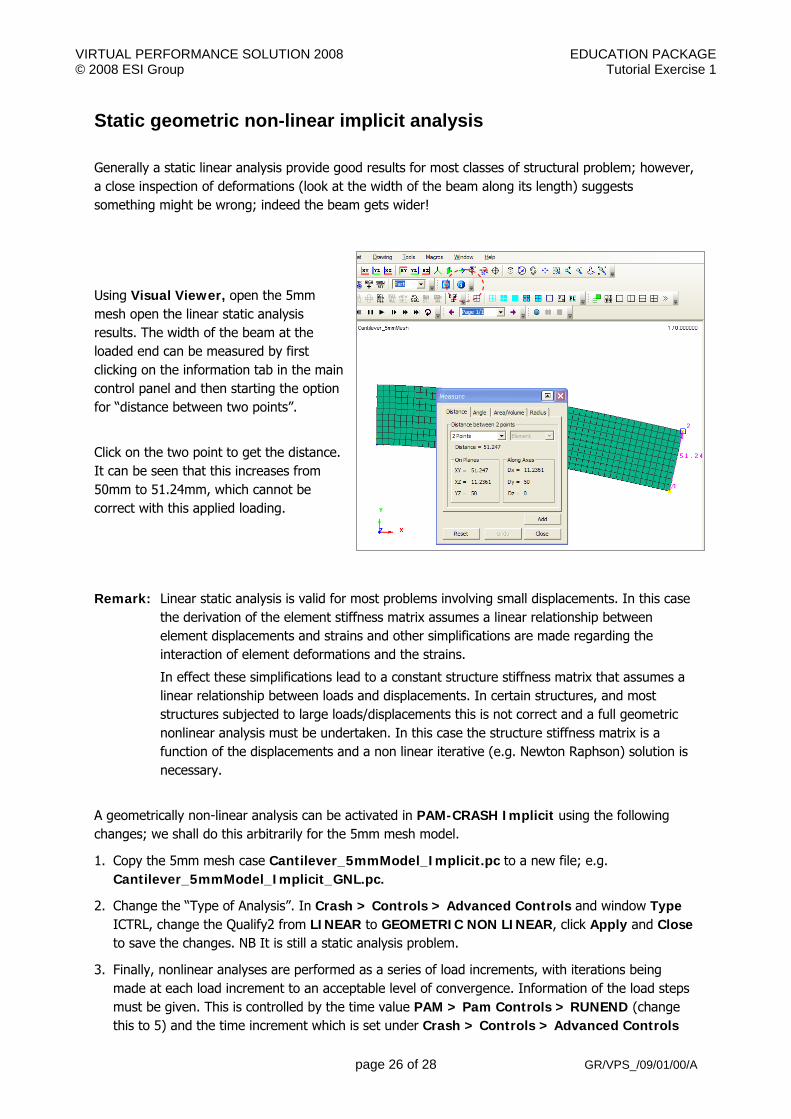
Static geometric non-linear implicit analysis

Generally a static linear analysis provide good results for most classes of structural problem; however, a close inspection of deformations (look at the width of the beam along its length) suggests something might be wrong; indeed the beam gets wider!

Using Visual Viewer, open the 5mm mesh open the linear static analysis results. The width of the beam at the loaded end can be measured by first clicking on the information tab in the main control panel and then starting the option for “distance between two points”.

Click on the two point to get the distance. It can be seen that this increases from 50mm to 51.24mm, which cannot be correct with this applied loading.

Remark: Linear static analysis is valid for most problems involving small displacements. In this case the derivation of the element stiffness matrix assumes a linear relationship between element displacements and strains and other simplifications are made regarding the interaction of element deformations and the strains.

In effect these simplifications lead to a constant structure stiffness matrix that assumes a linear relationship between loads and displacements. In certain structures, and most structures subjected to large loads/displacements this is not correct and a full geometric nonlinear analysis must be undertaken. In this case the structure stiffness matrix is a function of the displacements and a non linear iterative (e.g. Newton Raphson) solution is necessary.

A geometrically non-linear analysis can be activated in PAM-CRASH Implicit using the following changes; we shall do this arbitrarily for the 5mm mesh model.

1. Copy the 5mm mesh case Cantilever_5mmModel_Implicit.pc to a new file; e.g. Cantilever_5mmModel_Implicit_GNL.pc.

2. Change the “Type of Analysis”. In Crash > Controls > Advanced Controls and window Type ICTRL, change the Qualify2 from LINEAR to GEOMETRIC NON LINEAR, click Apply and Close to save the changes. NB It is still a static analysis problem.

3. Finally, nonlinear analyses are performed as a series of load increments, with iterations being made at each load increment to an acceptable level of convergence. Information of the load steps must be given. This is controlled by the time value PAM > Pam Controls > RUNEND (change this to 5) and the time increment which is set under Crash > Controls > Advanced Controls


page 27 of 28 GR/VPS_/09/01/00/A

and in the window Type for TCTRL (parameter DELTA, set this to 0.1). These two values mean that 50 load increments will be made.

4. Export the model to the file Cantilever_5mmModel_Implicit_GNL.pc and run the analysis with PAM-CRASH Implicit.

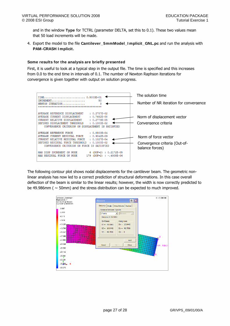
Some results for the analysis are briefly presented

First, it is useful to look at a typical step in the output file. The time is specified and this increases from 0.0 to the end time in intervals of 0.1. The number of Newton Raphson iterations for convergence is given together with output on solution progress.

The following contour plot shows nodal displacements for the cantilever beam. The geometric non-linear analysis has now led to a correct prediction of structural deformations. In this case overall deflection of the beam is similar to the linear results; however, the width is now correctly predicted to be 49.986mm ( ~ 50mm) and the stress distribution can be expected to much improved.

Norm of displacement vector

The solution time

Number of NR iteration for convergence

Convergence criteria

Norm of force vector

Convergence criteria (Out-of-balance forces)

Insert the back cover image in this header, then position and resize it !

vps 2008 educ example 1

Documents