VYSOKE UCENI TECHNICKE V BRNEBRNO UNIVERSITY OF TECHNOLOGY

FAKULTA INFORMACNICH TECHNOLOGIIUSTAV POCITACOVE GRAFIKY A MULTIMEDII

FACULTY OF INFORMATION TECHNOLOGYDEPARTMENT OF COMPUTER GRAPHICS AND MULTIMEDIA

AEROWORKS: POHYBOVA PLATFORMA PRO SIMULA-TORAEROWORKS: SIMULATOR MOTION PLATFORM

DIPLOMOVA PRACEMASTER’S THESIS

AUTOR PRACE Bc. MARTIN MORAVEKAUTHOR

VEDOUCI PRACE Ing. PETER CHUDY, Ph.D. MBASUPERVISOR

BRNO 2012

AbstraktTato diplomová práce se zabývá konceptem simulace letu s využitím Stewartovy platformya postupem výpočtu zpětné kinematiky tohoto manipulátoru. Dále je zde prezentovánprincip washout algoritmu, který zabezpečuje vhodné vnímání zrychlení a polohy pilotem vsimulátoru a zabraňuje tomu, aby platforma dosáhla svých limitů. Digitální filtry navrženépro použití v implementaci washout algoritmu a jejich charakteristiky jsou zde také popsány.Poslední část popisuje architekturu výsledného systému a implementaci jednotlivých částí.

AbstractThis diploma thesis is dealing with the concepts behind the Stewart platform based flightsimulation phenomena along with the method of inverse kinematics computation. Further,a washout algorithm to provide appropriate vestibular sensing to the pilot and ensuringthat platform will not reach its limits is presented. Digital filters designed to be used inthe implementation of the washout algorithm and their characteristics are also covered.The last part describes the architecture of the whole system and the implementation ofindividual parts.

Klíčová slovaStewartova platforma, paralelní manipulátor, letový simulátor, washout algoritmus.

KeywordsStewart platform, parallel manipulator, flight simulator, washout algorithm.

CitaceMartin Morávek: AeroWorks: Simulator Motion Platform, diplomová práce, Brno, FITVUT v Brně, 2012

AeroWorks: Simulator Motion Platform

AnnouncementI have written this Master thesis independently and without the aid of unfair or unautho-rized resources. Whenever content was taken directly or indirectly from other sources, thishas been indicated and the source referenced.

. . . . . . . . . . . . . . . . . . . . . . .Martin MorávekMay 18, 2012

AcknowledgementsI would like to thank my supervisor Ing. Peter Chudý Ph.D. MBA for his support and alsoDipl.-Ing. Andreas Jaroš for providing useful references.

c© Martin Morávek, 2012.Tato práce vznikla jako školní dílo na Vysokém učení technickém v Brně, Fakultě in-formačních technologií. Práce je chráněna autorským zákonem a její užití bez uděleníoprávnění autorem je nezákonné, s výjimkou zákonem definovaných případů.

Contents

1 Introduction 71.1 Purpose of Simulation . . . . . . . . . . . . . . . . . . . . . . . . . . . . . . 71.2 Advantages of Simulators . . . . . . . . . . . . . . . . . . . . . . . . . . . . 71.3 Categories of Simulators . . . . . . . . . . . . . . . . . . . . . . . . . . . . . 81.4 Motion Perception in Simulator . . . . . . . . . . . . . . . . . . . . . . . . . 81.5 Manipulators in Vehicle Simulators Overview . . . . . . . . . . . . . . . . . 9

1.5.1 Serial Manipulators . . . . . . . . . . . . . . . . . . . . . . . . . . . 101.5.2 Parallel Manipulators . . . . . . . . . . . . . . . . . . . . . . . . . . 10

2 History of Flight Simulation 112.1 Barrel Trainer . . . . . . . . . . . . . . . . . . . . . . . . . . . . . . . . . . . 112.2 Link Trainer . . . . . . . . . . . . . . . . . . . . . . . . . . . . . . . . . . . . 112.3 Beginning of Modern Flight Simulators . . . . . . . . . . . . . . . . . . . . . 12

2.3.1 Visual Systems . . . . . . . . . . . . . . . . . . . . . . . . . . . . . . 132.4 Modern Flight Simulation Design . . . . . . . . . . . . . . . . . . . . . . . . 13

3 Six Degree of Freedom Motion Platform 153.1 Origin of 6DOF Motion Platform . . . . . . . . . . . . . . . . . . . . . . . . 153.2 Platform Design and Geometry . . . . . . . . . . . . . . . . . . . . . . . . . 16

3.2.1 Influence of the Geometry . . . . . . . . . . . . . . . . . . . . . . . . 163.3 Inverse Kinematics . . . . . . . . . . . . . . . . . . . . . . . . . . . . . . . . 17

3.3.1 Inverse Kinematics Demonstration Application . . . . . . . . . . . . 193.4 Jacobian Matrix . . . . . . . . . . . . . . . . . . . . . . . . . . . . . . . . . 20

3.4.1 Jacobian of Stewart platform . . . . . . . . . . . . . . . . . . . . . . 203.4.2 Singularities . . . . . . . . . . . . . . . . . . . . . . . . . . . . . . . . 21

4 Washout Algorithm 224.1 Digital Filters in Washout Algorithm . . . . . . . . . . . . . . . . . . . . . . 22

4.1.1 FIR Filters . . . . . . . . . . . . . . . . . . . . . . . . . . . . . . . . 224.1.2 IIR Filters . . . . . . . . . . . . . . . . . . . . . . . . . . . . . . . . . 224.1.3 Digital Integrator . . . . . . . . . . . . . . . . . . . . . . . . . . . . . 23

4.2 Classical Washout Algorithm . . . . . . . . . . . . . . . . . . . . . . . . . . 234.3 Specific Digital filters in Classical Washout . . . . . . . . . . . . . . . . . . 25

5 Coordinate Systems 275.1 Aircraft Body Reference Frame . . . . . . . . . . . . . . . . . . . . . . . . . 27

5.1.1 Angles of Rotation in Body Reference Frame . . . . . . . . . . . . . 275.2 Simulator and Motion Platform Reference Frames . . . . . . . . . . . . . . 28

1

5.2.1 Platform World Reference Frame . . . . . . . . . . . . . . . . . . . . 285.2.2 Platform Body Reference Frame . . . . . . . . . . . . . . . . . . . . 295.2.3 Pilot’s Head Reference Frame . . . . . . . . . . . . . . . . . . . . . . 30

5.3 Earth-Centered Earth-Fixed Frame . . . . . . . . . . . . . . . . . . . . . . . 315.4 Earth-Centered Inertial Frame . . . . . . . . . . . . . . . . . . . . . . . . . 32

6 Aircraft motion in 6DOF 336.1 Translational Motion . . . . . . . . . . . . . . . . . . . . . . . . . . . . . . . 336.2 Angular Motion . . . . . . . . . . . . . . . . . . . . . . . . . . . . . . . . . . 346.3 Static Equilibrium . . . . . . . . . . . . . . . . . . . . . . . . . . . . . . . . 35

6.3.1 Stability-axes Coordinate System . . . . . . . . . . . . . . . . . . . . 356.3.2 Equilibrium Analysis . . . . . . . . . . . . . . . . . . . . . . . . . . . 35

7 Requirements 377.1 Simulator Categories . . . . . . . . . . . . . . . . . . . . . . . . . . . . . . . 377.2 Motion System Requirements . . . . . . . . . . . . . . . . . . . . . . . . . . 38

7.2.1 Motion System Responses . . . . . . . . . . . . . . . . . . . . . . . . 38

8 Implementation 398.1 Used Tools . . . . . . . . . . . . . . . . . . . . . . . . . . . . . . . . . . . . 39

8.1.1 Qt Framework . . . . . . . . . . . . . . . . . . . . . . . . . . . . . . 398.1.2 Qwt Library . . . . . . . . . . . . . . . . . . . . . . . . . . . . . . . 398.1.3 FSUIPC: Application Interfacing Module for Microsoft Flight Simulator 398.1.4 Microsoft Flight Simulator X . . . . . . . . . . . . . . . . . . . . . . 398.1.5 Matlab . . . . . . . . . . . . . . . . . . . . . . . . . . . . . . . . . . 408.1.6 Testing Configuration . . . . . . . . . . . . . . . . . . . . . . . . . . 40

8.2 AeroWorks 6DOF Motion Platform Model . . . . . . . . . . . . . . . . . . . 408.2.1 Pololu Mini Maestro 12-channel USB Servo Controller . . . . . . . . 408.2.2 Savox Digital Servos . . . . . . . . . . . . . . . . . . . . . . . . . . . 42

8.3 Final System Arrangement . . . . . . . . . . . . . . . . . . . . . . . . . . . 438.4 PC Section . . . . . . . . . . . . . . . . . . . . . . . . . . . . . . . . . . . . 438.5 Control Application . . . . . . . . . . . . . . . . . . . . . . . . . . . . . . . 43

8.5.1 Digital Filter Class . . . . . . . . . . . . . . . . . . . . . . . . . . . . 448.5.2 Plots . . . . . . . . . . . . . . . . . . . . . . . . . . . . . . . . . . . . 448.5.3 Communication with the Motion Platform . . . . . . . . . . . . . . . 458.5.4 AeroWorks Communication Protocol . . . . . . . . . . . . . . . . . 458.5.5 State Indicators . . . . . . . . . . . . . . . . . . . . . . . . . . . . . . 45

8.6 Platform Section . . . . . . . . . . . . . . . . . . . . . . . . . . . . . . . . . 468.7 Aircraft Manoeuvres, their Output and Sensing . . . . . . . . . . . . . . . . 47

8.7.1 Takeoff . . . . . . . . . . . . . . . . . . . . . . . . . . . . . . . . . . 478.7.2 High-frequency Vibrations . . . . . . . . . . . . . . . . . . . . . . . . 488.7.3 Landing . . . . . . . . . . . . . . . . . . . . . . . . . . . . . . . . . . 498.7.4 Aircraft Roll Rotations . . . . . . . . . . . . . . . . . . . . . . . . . 49

9 Conclusion 51

A CD Contents 54

B Control Application Screenshot 55

2

List of Figures

1.1 Vestibular System . . . . . . . . . . . . . . . . . . . . . . . . . . . . . . . . 91.2 Heli Trainer – a serial manipulator simulator . . . . . . . . . . . . . . . . . 91.3 Example of a simulator with 6DOF motion platform . . . . . . . . . . . . . 10

2.1 Barrel trainer for Antoinette monoplane . . . . . . . . . . . . . . . . . . . . 112.2 The Link Trainer and instructors desk . . . . . . . . . . . . . . . . . . . . . 122.3 Comet 4 simulator with pitch motion system . . . . . . . . . . . . . . . . . 132.4 Modern flight simulation block scheme . . . . . . . . . . . . . . . . . . . . . 14

3.1 Stewart’s model of simulator platform with linear co-ordinage leg system . . 153.2 Gough’s tyre testing machine . . . . . . . . . . . . . . . . . . . . . . . . . . 163.3 The first flight simulator based on an octahedral hexapod . . . . . . . . . . 173.4 Stewart platform architectures . . . . . . . . . . . . . . . . . . . . . . . . . 183.5 Simple Stewart platform scheme . . . . . . . . . . . . . . . . . . . . . . . . 193.6 Inverse kinematics demonstration application . . . . . . . . . . . . . . . . . 20

4.1 Finite impulse response filter scheme . . . . . . . . . . . . . . . . . . . . . . 234.2 Infinite impulse response filter scheme . . . . . . . . . . . . . . . . . . . . . 234.3 Digital integrator filter scheme . . . . . . . . . . . . . . . . . . . . . . . . . 234.4 Filtering aircraft motions . . . . . . . . . . . . . . . . . . . . . . . . . . . . 244.5 Classical washout algorithm . . . . . . . . . . . . . . . . . . . . . . . . . . . 254.6 Washout filter response . . . . . . . . . . . . . . . . . . . . . . . . . . . . . 254.7 Washout filters response . . . . . . . . . . . . . . . . . . . . . . . . . . . . . 26

5.1 Aircraft body reference frame . . . . . . . . . . . . . . . . . . . . . . . . . . 285.2 Pitch, roll and yaw angles of rotation . . . . . . . . . . . . . . . . . . . . . . 295.3 Platform reference frames . . . . . . . . . . . . . . . . . . . . . . . . . . . . 305.4 Earth-Centered Earth-Fixed Frame . . . . . . . . . . . . . . . . . . . . . . . 315.5 Earth-Centered Inertial Frame . . . . . . . . . . . . . . . . . . . . . . . . . 32

6.1 Equilibrium quantities diagram . . . . . . . . . . . . . . . . . . . . . . . . . 36

8.1 AeroWorks 6DOF motion platform model . . . . . . . . . . . . . . . . . . . 418.2 Pololu Mini Maestro 12-channel USB servo controller . . . . . . . . . . . . . 428.3 System scheme using FSUIPC . . . . . . . . . . . . . . . . . . . . . . . . . . 438.4 Matlab 1–D filter scheme . . . . . . . . . . . . . . . . . . . . . . . . . . . . 448.5 System scheme using AeroWorks communication protocol . . . . . . . . . . 468.6 Control application indicators . . . . . . . . . . . . . . . . . . . . . . . . . . 478.7 Algorithm behaviour at high-frequency vibrations . . . . . . . . . . . . . . . 478.8 Algorithm behaviour at take off . . . . . . . . . . . . . . . . . . . . . . . . . 48

3

8.9 Algorithm behaviour at landing . . . . . . . . . . . . . . . . . . . . . . . . . 498.10 Algorithm behaviour at roll rotations . . . . . . . . . . . . . . . . . . . . . . 50

4

Nomenclature

aAA aircraft acceleration in body reference frame

fAA aircraft specific force in body reference frame

gA gravitational acceleration in body reference frame

ωAA aircraft angular velocities in body reference frame

TS transformation matrix from angular velocity to euler angle rates

LIS body frame to inertial frame rotation matrix

po vehicle position relative to ECI frame

vi velocity of vehicle in Fi

ve velocity of vehicle in ECEF frame

ωe/i angular velocity of ECEF frame in respect to Fi

m mass of vehicle

FA,T vector sum of aerodynamic and thrust forces

MA,T sum of aerodynamics and thrust moment about the centre of mass

h angular momentum vector in Fi

Fi an inertial reference frame

Fb body fixed reference frame

frl fuselage reference line

αfrl angle of attack measured to the frl

αT angle between mathbfFT and frl

FT thrust vector

FR resultant aerodynamic force on aircraft

L lift component of FR

D drag component of FR

R aircraft reference point

C center of mass

T horizontal tail point

5

MR total aerodynamic moment at R

MCM moment at centre of mass

Mp pitching moment created directly by the engines

FN normal force

FX axial force

S total wing area

c mean aerodynamic chord

q dynamic pressure

ECEF Earth-centered Earth-fixed Frame

ECI Earth-centered Inertial Frame

IAS Indicated Air Speed

FCS (Integrated) Fligh Control System

FAA Federal Aviation Administration

FTD Flight Training Device

FFS Full Flight Simulator

AOA Angle of Attack

UI User Interface

FSX Microsoft Flight Simulator X

6

Chapter 1

Introduction

Due to the progress of computing and computer visualization in the end of 20th centurycomputer-controlled simulators have become widely spread. Simulators can be used in awide range of areas, simulating practically any type of vehicle – ground vehicles, ships,aerial vehicles or aerospace spacecrafts.

1.1 Purpose of Simulation

The aim of simulator is to provide similar or the same stimuli to operator’s senses as a realvehicle would. Real vehicle moves along six-dimensional trajectory (3 translational and 3rotational coordinates) from one place to another which can be hundreds of kilometres farapart. On the other hand, simulator’s location is stationary and its workspace is quitelimited. Considering these facts, simulator motion must be very well planned and one cannot simply copy the motions of a real vehicle.

1.2 Advantages of Simulators

There are many obvious advantages of operating simulators over the real vehicles such as

• Safety - vehicle crew can not be harmed while using simulator no matter how badlyis the vehicle operated, also no damage to the simulator or vehicle is possible.

• Training and research - Simulator can be used not only for training which includesbasic control, but also for handling specific critical scenarios which will be hard toinduce in real conditions, or inducing these scenarios would be unacceptably haz-ardous. Practically, any situation and conditions can be simulated, such as variousvehicle setup, different types of environments (weather) or any imaginable failure orserie of failures.

• Running costs - in many cases the running costs of simulator are significantly lowerthan using a real vehicle.

7

1.3 Categories of Simulators

According to [2] simulators can be divided into three categories:

• Engineering (Vehicle Design Simulators) - Serve to examine the properties of humansin general as controllers of given vehicle properties. In the ideal case, the simulationenvironment is considered equivalent to the vehicle environment, allowing perceptionof all of the stimuli as they would occur in the vehicle.

• Research (Simulator Design) Simulators - Serve to examine the properties of humansin general as controllers of given vehicle properties, or to evaluate the effectiveness ofthe simulation in reacting the stimulus environment of the vehicle.

• Examination or Training Simulators - Serve to examine the capabilities of one par-ticular controller with regard to the control of a specific vehicle type, or to developthe skills required by one particular controller in order to control a specific vehicletype.

1.4 Motion Perception in Simulator

The aim of all simulator designers is to offer as realistic simulator impression as possible.There are several ways to achieve this goal. Humans perceive their surrounding throughtheir senses, and the more the sensations in simulator are similar to the sensations in realvehicle, the more realistic the simulator is. Now consider the human senses perception in avehicle simulator and their according inputs.

• Eyesight - considerable part of information about our surroudings is being sensed byour eyes. In simulator this includes especially visualization of vehicle surroundings(generated by computer visualization and 3D graphics) but also an interior of sim-ulator cabin or cockpit as well as the appearance of all kinds of indicators, switchesand displays located on instrument panel. Also the look of other visible componentsas signs and writings is important .

• Hearing - every vehicle produces different kinds of sounds and noises depending onvehicle condition and settings, outer environment and many others. Generating ve-hicle sound should not be neglected in a simulator as sensing these sounds is addingextra information to vehicle operator and improves simulator plausibility.

• Sense of touch - everytime we touch something we sense its surface. In simulatorcabin the same materials as in the real vehicle should be used (mainly on the surfacepilot use to touch while operating the vehicle). This sense is also partially responsiblefor sensing vibrations.

• Olfactory sense - every environment has its specific smell. Olfaction also helps recog-nize different kinds of situations, for example a case of fire or some liquid leakage.

• Vestibular system - vestibular system is responsible for sensing human head linearand angular accelerations. According to [20] , the endolymph of each canal(posterior,anterior, lateral) is continuous with that in the utriculus at one end, and separatedfrom it at the other end by a flexible mechanosensitive barrier called the crista am-pullaris. Crista ampullaris is particularly sensitive to changes in angular acceleration

8

and deceleration of the head. Otolith receptors respond to linear acceleration anddeceleration of the head. This all is located in the inner ear.

Vestibular system sensing in simulator is what we want to improve using a 6 degree-of-freedom motion-platform based simulator.

Figure 1.1: Vestibular system [20] and Crista Ampullaris[30].

1.5 Manipulators in Vehicle Simulators Overview

Manipulators in vehicle simulators are used to stimulate human motion perception andthereby increase the simulation’s plausibility.

Figure 1.2: Heli Trainer – a serial manipulator simulator [19].

9

1.5.1 Serial Manipulators

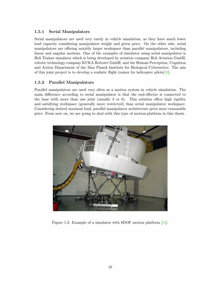
Serial manipulators are used very rarely in vehicle simulation, as they have much lowerload capacity considering manipulator weight and given price. On the other side, serialmanipulators are offering notably larger workspace than parallel manipulators, includinglinear and angular motions. One of the examples of simulator using serial manipulator isHeli Trainer simulator which is being developed by aviation company Heli Aviation GmbH,robotic technology company KUKA Roboter GmbH, and the Human Perception, Cognitionand Action Department of the Max Planck Institute for Biological Cybernetics. The aimof this joint project is to develop a realistic flight trainer for helicopter pilots[19].

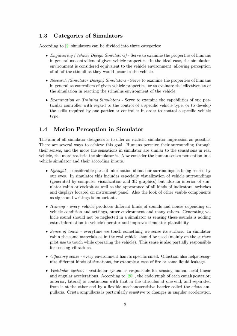
1.5.2 Parallel Manipulators

Parallel manipulators are used very often as a motion system in vehicle simulation. Themain difference according to serial manipulator is that the end-effector is connected tothe base with more than one joint (usually 3 or 6). This solution offers high rigidityand satisfying workspace (generally more restricted) than serial manipulator workspace.Considering desired maximal load, parallel manipulator architecture gives more reasonableprice. From now on, we are going to deal with this type of motion-platform in this thesis.

Figure 1.3: Example of a simulator with 6DOF motion platform [18].

10

Chapter 2

History of Flight Simulation

2.1 Barrel Trainer

Early flight simulators were very simple devices constructed mostly of wood. Their mainpurpose was to help the pilot to get familiar with airplane controls.First flight simulator was Antoinette Barrel Trainer served to train pilots for the An-

toinette monoplane. It was operated by two wheels – one for controlling pitch and one forroll. As can be seen on fig. 2.1, pilot was sitting on a half of barrel which could be tilted bytwo men standing next to the device according the movement of control elements. Despitethe fact that this first simulator was very simple, it served its purpose.

Figure 2.1: Barrel trainer for Antoinette monoplane[26].

2.2 Link Trainer

Later, Ed Link who had not been satisfied by obtaining his pilot licence process that tookseveral years developed a more sophisticated training device named after him The LinkTrainer. Patent for this device was granted in 1931. Ed Link opened a flying school in

11

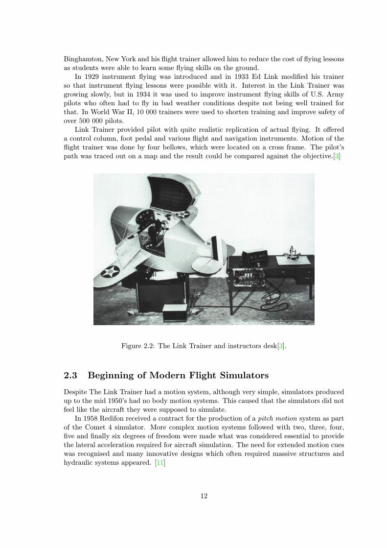
Binghamton, New York and his flight trainer allowed him to reduce the cost of flying lessonsas students were able to learn some flying skills on the ground.In 1929 instrument flying was introduced and in 1933 Ed Link modified his trainer

so that instrument flying lessons were possible with it. Interest in the Link Trainer wasgrowing slowly, but in 1934 it was used to improve instrument flying skills of U.S. Armypilots who often had to fly in bad weather conditions despite not being well trained forthat. In World War II, 10 000 trainers were used to shorten training and improve safety ofover 500 000 pilots.Link Trainer provided pilot with quite realistic replication of actual flying. It offered

a control column, foot pedal and various flight and navigation instruments. Motion of theflight trainer was done by four bellows, which were located on a cross frame. The pilot’spath was traced out on a map and the result could be compared against the objective.[3]

Figure 2.2: The Link Trainer and instructors desk[3].

2.3 Beginning of Modern Flight Simulators

Despite The Link Trainer had a motion system, although very simple, simulators producedup to the mid 1950’s had no body motion systems. This caused that the simulators did notfeel like the aircraft they were supposed to simulate.In 1958 Redifon received a contract for the production of a pitch motion system as part

of the Comet 4 simulator. More complex motion systems followed with two, three, four,five and finally six degrees of freedom were made what was considered essential to providethe lateral acceleration required for aircraft simulation. The need for extended motion cueswas recognised and many innovative designs which often required massive structures andhydraulic systems appeared. [11]

12

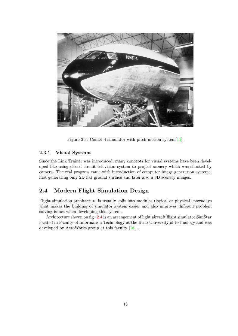
Figure 2.3: Comet 4 simulator with pitch motion system[11].

2.3.1 Visual Systems

Since the Link Trainer was introduced, many concepts for visual systems have been devel-oped like using closed circuit television system to project scenery which was shooted bycamera. The real progress came with introduction of computer image generation systems,first generating only 2D flat ground surface and later also a 3D scenery images.

2.4 Modern Flight Simulation Design

Flight simulation architecture is usually split into modules (logical or physical) nowadayswhat makes the building of simulator system easier and also improves different problemsolving issues when developing this system.Architecture shown on fig. 2.4 is an arrangement of light aircraft flight simulator SimStar

located in Faculty of Information Technology at the Brno University of technology and wasdeveloped by AeroWorks group at this faculty [16] .

13

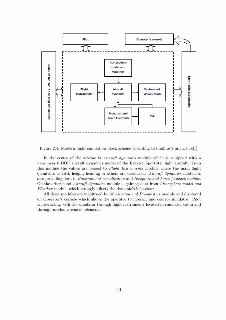
Figure 2.4: Modern flight simulation block scheme according to SimStar’s archicture[5].

In the centre of the scheme is Aircraft dynamics module which is equipped with anon-linear 6 DOF aircraft dynamics model of the Evektor SportStar light aircraft. Fromthis module the values are passed to Flight Instruments module where the main flightquantities as IAS, height, heading or others are visualized. Aircraft dynamics module isalso providing data to Environment visualization and Inceptors and Force feedback module.On the other hand Aircraft dynamics module is gaining data from Atmosphere model andWeather module which strongly affects the dynamic’s behaviour.All these modules are monitored by Monitoring and Diagnostics module and displayed

on Operator’s console which allows the operator to interact and control simulator. Pilotis interacting with the simulator through flight instruments located in simulator cabin andthrough mechanic control elements.

14

Chapter 3

Six Degree of Freedom MotionPlatform

3.1 Origin of 6DOF Motion Platform

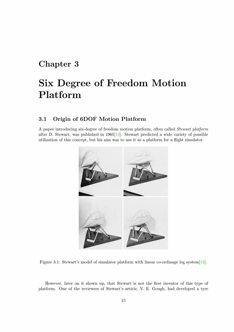
A paper introducing six-degree of freedom motion platform, often called Stewart platformafter D. Stewart, was published in 1965[14]. Stewart predicted a wide variety of possibleutilization of this concept, but his aim was to use it as a platform for a flight simulator.

Figure 3.1: Stewart’s model of simulator platform with linear co-ordinage leg system[14].

However, later on it shown up, that Stewart is not the first inventor of this type ofplatform. One of the reviewers of Stewart’s article, V. E. Gough, had developed a tyre

15

testing machine[6] which had a 6 legs and 6DOF motion platform similar to the Stewart’sone sooner, in 1949. Despite this fact, six degree of freedom motion platform is nowadaysusually called after Stewart.

Figure 3.2: Gough’s tyre testing machine, photo published in review of Stewart’s paper[14].

Third man, that must be taken into consideration is Klaus Cappel, an engineer fromUnited States. In 1962, before Stewart’s paper was published, Cappel had come with a6DOF platform arrangement, which was the same as Mr. Cough’s[4]. Later, Cappel wasasked to design and construct a 6DOF helicopter flight simulator for Sikorsky Aircraft Di-vision of United Technologies. This was the first flight simulator using octahedral hexapodarrangement.

3.2 Platform Design and Geometry

Platform designer is free to choose joints arrangement, leg lengths, upper and lower platformplate diameters, different type of actuators such as electric or hydraulic and many others.This all has considerable effect on platform’s workspace, rigidity and speed.

3.2.1 Influence of the Geometry

Optimal platform geometry depends on the purpose of platform. Considering a flightsimulator, having wide range of linear and angular motions can be useful. A lot has beenwritten on determining platform’s workspace, however this is not a simple task, especiallywith parallel manipulators. For our purpose, one of the designs developed in [12] can beused.

16

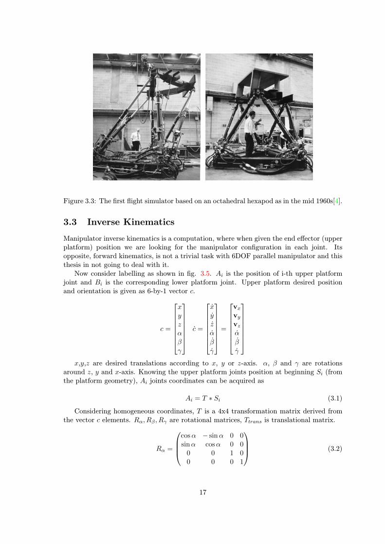
Figure 3.3: The first flight simulator based on an octahedral hexapod as in the mid 1960s[4].

3.3 Inverse Kinematics

Manipulator inverse kinematics is a computation, where when given the end effector (upperplatform) position we are looking for the manipulator configuration in each joint. Itsopposite, forward kinematics, is not a trivial task with 6DOF parallel manipulator and thisthesis in not going to deal with it.Now consider labelling as shown in fig. 3.5. Ai is the position of i-th upper platform

joint and Bi is the corresponding lower platform joint. Upper platform desired positionand orientation is given as 6-by-1 vector c.

c =

xyzαβγ

c =

xyzα

βγ

=

vx

vy

vz

α

βγ

x,y,z are desired translations according to x, y or z-axis. α, β and γ are rotations

around z, y and x-axis. Knowing the upper platform joints position at beginning Si (fromthe platform geometry), Ai joints coordinates can be acquired as

Ai = T ∗ Si (3.1)

Considering homogeneous coordinates, T is a 4x4 transformation matrix derived fromthe vector c elements. Rα, Rβ, Rγ are rotational matrices, Ttrans is translational matrix.

Rα =

cosα − sinα 0 0sinα cosα 0 00 0 1 00 0 0 1

(3.2)

17

Figure 3.4: Stewart platform architectures that yield optimal dexterity[12].

Rβ =

cosβ 0 sinβ 00 1 0 0

− sinβ 0 cosβ 00 0 0 1

(3.3)

Rγ =

1 0 0 00 cos γ − sin γ 00 sin γ cos γ 00 0 0 1

(3.4)

Ttrans =

0 0 0 x0 0 0 y0 0 0 z0 0 0 1

(3.5)

T = Rα ∗Rβ ∗Rγ ∗ Ttrans (3.6)

T =

cosα cosβ cosα sinβ sin γ − sinα cos γ) cosα sinβ cos γ + sinα sin γ xsinα cosβ sinα sinβ sin γ + cosα cos γ sinα sinβ cos γ − cosα sin γ y− sinβ cosβ sin γ cosβ cos γ z

0 0 0 1

(3.7)

Now, knowing all upper platform joints coordinates Ai and base platform points Bi

(vectors has 4 elements as we are using homogeneous coordinates), we can simply obtainlength of each actuator leg li.

Ai = [xai , yai , zai , 1] (3.8)

18

Figure 3.5: Simple Stewart platform scheme.

Bi = [xbi , ybi , zbi , 1] (3.9)

li = ‖Ai −Bi‖ =√

(xai − xbi)2 + (yai − ybi)

2 + (zai − zbi)2 (3.10)

As Stewart platform has only prismatic joints, by deriving the leg lengths we havecomputed complete inverse kinematics of robot (configuration for every joint of the manip-ulator).

3.3.1 Inverse Kinematics Demonstration Application

We have developed a demonstration application for inverse kinematics problem. This appli-cation runs in Matlab [21] environment and it is using the computation method describedabove. The inputs are 3 rotation values (pitch, roll, yaw) and 3 translation values. Outputsare computed leg lengths and Stewart platform schematic representation.For setting platform configuration 6 sliders are used(3 for rotation, 3 for translation).

When value of any of these sliders is changed, a new computation is triggered. At firstpoints that represent platform in neutral configuration are created (3 for upper platformand 3 bottom platform). Then a 4 × 4 transformation matrix is generated by functiongenTmatrix using the values from sliders. All upper platform points are multiplied withthis generated matrix to obtain points position at the new configuration.In the end of computation the length for each linear actuator is computed (as described

above), upper and bottom platforms are rendered together with linear actuators. Finally,camera position, orientation and viewing angle is set up so that the whole platform wouldbe visible.

19

Figure 3.6: Inverse kinematics demonstration application.

3.4 Jacobian Matrix

In robotics, the Jacobian matrix maps the rates of change of position of the end effector(in this case upper platform), to the rates of change of the joints. This means, that theJacobian indicates the effort with which the end effector position can be changed as afunction of actuators configuration[2].

3.4.1 Jacobian of Stewart platform

For Stewart platform is Jacobian matrix defined as

JT =

∂l1∂x

∂l1∂y

∂l1∂z

∂l1∂α

∂l1∂β

∂l1∂γ

∂l2∂x

∂l2∂y

∂l2∂z

∂l2∂α

∂l2∂β

∂l2∂γ

∂l3∂x

∂l3∂y

∂l3∂z

∂l3∂α

∂l3∂β

∂l3∂γ

∂l4∂x

∂l4∂y

∂l4∂z

∂l4∂α

∂l4∂β

∂l4∂γ

∂l5∂x

∂l5∂y

∂l5∂z

∂l5∂α

∂l5∂β

∂l5∂γ

∂l6∂x

∂l6∂y

∂l6∂z

∂l6∂α

∂l6∂β

∂l6∂γ

(3.11)

The relation between leg length changes ∆l and end effector position changes ∆c canbe given as

∆l = J ∗∆c (3.12)

or with platform and joint ratesl = J ∗ c (3.13)

20

dl1dl2dl3dl4dl5dl6

= J ∗

dxdydzdαdβdγ

(3.14)

where[dx dy dz

]Tis differentiation of position vector. This differentiation we un-

derstand as dxdydz

=d

dtP = lim

∆t→0

P (t+∆t)− P (t))

∆t(3.15)

where P is the position vector

P =

xyz

(3.16)

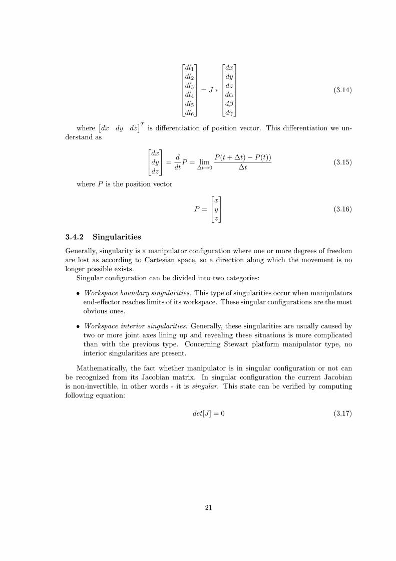
3.4.2 Singularities

Generally, singularity is a manipulator configuration where one or more degrees of freedomare lost as according to Cartesian space, so a direction along which the movement is nolonger possible exists.Singular configuration can be divided into two categories:

• Workspace boundary singularities. This type of singularities occur when manipulatorsend-effector reaches limits of its workspace. These singular configurations are the mostobvious ones.

• Workspace interior singularities. Generally, these singularities are usually caused bytwo or more joint axes lining up and revealing these situations is more complicatedthan with the previous type. Concerning Stewart platform manipulator type, nointerior singularities are present.

Mathematically, the fact whether manipulator is in singular configuration or not canbe recognized from its Jacobian matrix. In singular configuration the current Jacobianis non-invertible, in other words - it is singular. This state can be verified by computingfollowing equation:

det[J ] = 0 (3.17)

21

Chapter 4

Washout Algorithm

The aim of simulator motion platform is to provide appropriate information to the vestibularsystem of a pilot. Compared to the real airplane, the motion platform workspace is verylimited and providing these sensings can be a tricky issue. To ensure that motion platformwill not reach it’s workspace envelope and sufficiently plausible vestibular sensings will beperceived by pilot a washout algorithm is being used.

4.1 Digital Filters in Washout Algorithm

Digital filter is a system which process discrete signal. This signal is sampled on certainfrequency FS and can be represented as array of discrete values. Digital filter can beimplemented by cascading simple blocks. These are:

•∑- summation block which sums up all inputs resulting to one output value

• z−1 - delay block

• bn - multiplication with constant block (used with previous inputs)

• am - multiplication with constant block (used with previous outputs)

If N is the number of bn multiplication blocks and M is the number of am blocks, thenthe filter order is the higher one of these values. By the length of impulse response thedigital filters are divided into two categories - FIR (finite impulse response) and IIR (infiniteimpulse response) filters.

4.1.1 FIR Filters

As shown in fig. 4.1, FIR filter is dealing only with previous input samples. This meansthat the impulse response of Nth order FIR filter lasts N + 1 samples and then goes zero.

4.1.2 IIR Filters

IIR filter output depends not only on previous inputs, but also on previous outputs. Thismakes IIR filter impulse response infinite in time, and also much harder to design IIR filtercoefficients than FIR filter coefficients.

22

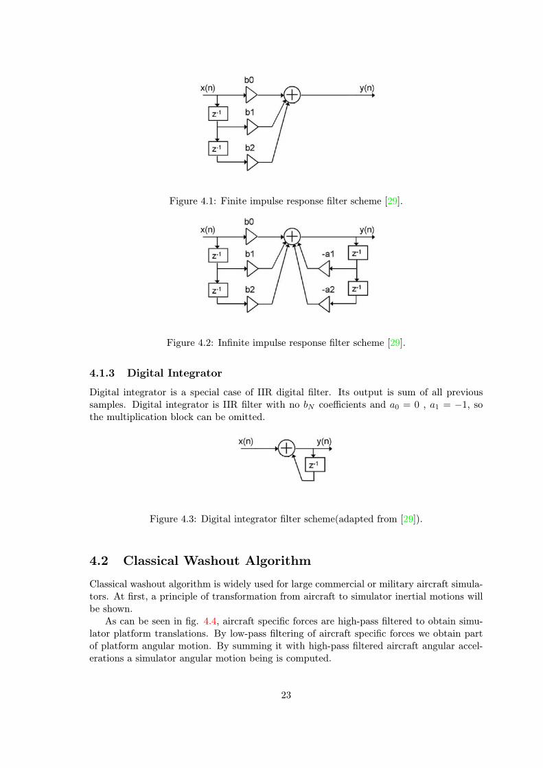
Figure 4.1: Finite impulse response filter scheme [29].

Figure 4.2: Infinite impulse response filter scheme [29].

4.1.3 Digital Integrator

Digital integrator is a special case of IIR digital filter. Its output is sum of all previoussamples. Digital integrator is IIR filter with no bN coefficients and a0 = 0 , a1 = −1, sothe multiplication block can be omitted.

Figure 4.3: Digital integrator filter scheme(adapted from [29]).

4.2 Classical Washout Algorithm

Classical washout algorithm is widely used for large commercial or military aircraft simula-tors. At first, a principle of transformation from aircraft to simulator inertial motions willbe shown.As can be seen in fig. 4.4, aircraft specific forces are high-pass filtered to obtain simu-

lator platform translations. By low-pass filtering of aircraft specific forces we obtain partof platform angular motion. By summing it with high-pass filtered aircraft angular accel-erations a simulator angular motion being is computed.

23

Figure 4.4: Filtering aircraft motions to yield simulator inertial motion cues[2].

Filter ωn [Hz]x translational high-pass 2.5y and z translational high-pass 4.0All rotational high-pass 1.0x translational low-pass 5.0y translational low-pass 8.0

Table 4.1: Recommended washout filters cut-off frequencies[9].

Now a solution for classical washout will be shown as described in [9]. Inputs of thealgorithm are the aircraft cockpit specific forces and the aircraft angular rates. Aircraftspecific forces are defined as fAA = aAA− gA. These forces are high-pass filtered to acquiresimulator translational accelerations. Low frequency aircraft forces have to be filtered out asthey would result in big translational movements of platform and motion base would reachits workspace limits. Accelerations are integrated twice to obtain a platform position.Aircraft specific forces are also passed to low-pass filter, then scaled and rate-limited so

the pitch and roll angles are produced. This technique is called tilt-coordination. The aimis to orient the gravity vector by tilting the platform, relative to pilot’s head same as thelow-frequency specific force would in the real aircraft. Tilt-coordination will allow simulat-ing continuous accelerations without reaching simulator’s limits. However, this techniquecannot be used to simulate continuous vertical acceleration due to obvious reasons and lackof vertical acceleration sensing can be noted.The aircraft angular rates ωAA are high-pass filtered to yield the high-frequency compo-

nent of simulator angular rates (low-frequency component is supplied by tilt-coordinationtechnique). After filtering the angular rates are integrated once to obtain the platformangles.

24

Figure 4.5: Classical washout algorithm presented in [9].

4.3 Specific Digital filters in Classical Washout

In this section specific digital high-pass and low-pass filters that will be used in implemen-tation of classical washout algorithm are presented . Filters are 9th order FIR filters withmultiplication coefficients designed using Matlab software[21]. We decided to use FIR fil-ters concept for its small and constant group delay, and their simplicity. Filter’s magnituderesponse is shown in fig. 4.7 and 4.6. Assume, that the system will be using the samplingfrequency of 40Hz.

Figure 4.6: Washout filter response.

25

Figure 4.7: Washout filters response.

26

Chapter 5

Coordinate Systems

Coordinate systems (or Frames of Reference) and conversion between them are widelyused in aerospace field and are considered as fundamentals. In the process of implementingwashout algorithm and the motion platform control designer must be aware of differentframes of reference and the relationship between them. Coordinate systems described inthis thesis are considered to be standards according to [10] and [7].

5.1 Aircraft Body Reference Frame

Origin of the aircraft body coordinate frame is in the reference point of the aircraft (usuallyat the centre of mass). Translation of this coordinate frame is the same as translation ofaircraft reference point and the frame is rotating in the same way as the rigid body aircraft.

• x-axis is pointing towards the aircraft nose in the symmetry plane.

• y-axis is pointing to the right wing to form a righ hand coordinate system with othertwo axis.

• z-axis is pointing downwards in the symmetry plane of the aircraft.

5.1.1 Angles of Rotation in Body Reference Frame

Considering aircraft body reference frame rotations around x, y and z axis are possible.Positive direction of rotation is according to right hand rule(when right hand’s thumb ispointing in the direction of rotation axis, then the other bended fingers of this hand areindicating positive sense of rotation around this axis).

• Pitch is rotation around y-axis.

• Roll is rotation around x-axis and it is often denoted as bank angle.

• Yaw is rotation around z-axis. It is represented by the heading angle.

27

Figure 5.1: Aircraft body reference frame (adapted from [27]).

5.2 Simulator and Motion Platform Reference Frames

There are three different coordinate frames with the simulator motion platform itself.

5.2.1 Platform World Reference Frame

Origin of the world reference frame is in the centre of base platform and it is fixed to it.Index of World reference frame is W.

• x-axis is pointing forward.

• y-axis is chosen to form a right hand coordinate system with x and y axis.

• z-axis is pointing downwards in the direction of gravity.

28

Figure 5.2: Pitch, roll and yaw angles of rotation[15].

5.2.2 Platform Body Reference Frame

Origin of the platform body reference frame is in the centre of upper (moving) platformand it is translating and rotating with this platform. Transformation from world referenceframe to body reference frame can be obtained from the platform configuration and will bea combination of translation and also rotation. Index of this frame is b.

• x-axis is pointing forward in the direction of upper platform.

• y-axis is chosen to form a right hand coordinate system with x and z-axis.

• z-axis is pointing downwards perpendicularly to the plane of upper platform.

29

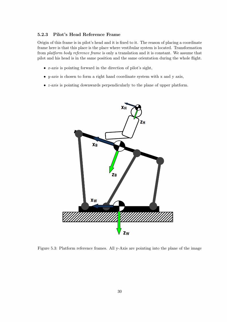
5.2.3 Pilot’s Head Reference Frame

Origin of this frame is in pilot’s head and it is fixed to it. The reason of placing a coordinateframe here is that this place is the place where vestibular system is located. Transformationfrom platform body reference frame is only a translation and it is constant. We assume thatpilot and his head is in the same position and the same orientation during the whole flight.

• x-axis is pointing forward in the direction of pilot’s sight,

• y-axis is chosen to form a right hand coordinate system with x and y axis,

• z-axis is pointing downwards perpendicularly to the plane of upper platform.

Figure 5.3: Platform reference frames. All y-Axis are pointing into the plane of the image

30

5.3 Earth-Centered Earth-Fixed Frame

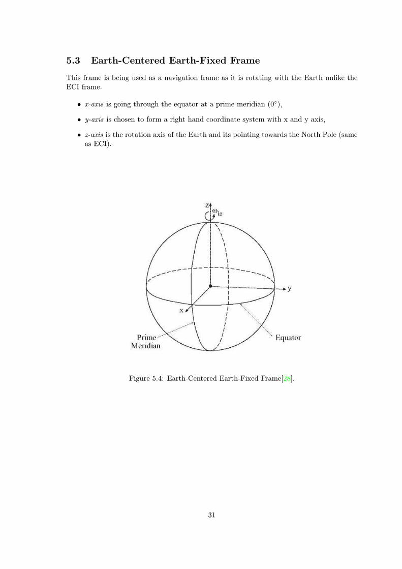
This frame is being used as a navigation frame as it is rotating with the Earth unlike theECI frame.

• x-axis is going through the equator at a prime meridian (0),

• y-axis is chosen to form a right hand coordinate system with x and y axis,

• z-axis is the rotation axis of the Earth and its pointing towards the North Pole (sameas ECI).

Figure 5.4: Earth-Centered Earth-Fixed Frame[28].

31

Figure 5.5: Earth-Centered Inertial Frame[8].

5.4 Earth-Centered Inertial Frame

Origin of this frame is the centre of the Earth. It is not rotating with the Earth.

• x-axis is pointing in direction of vernal equinox(from the center of the Earth to thecentre of the Sun),

• y-axis is chosen to form a right hand coordinate system with x and y axis,

• z-axis is the rotation axis of the Earth and its pointing towards the North Pole.

32

Chapter 6

Aircraft motion in 6DOF

During the flight the aircraft is executing a complex spatial motion. This motion is a6 degree-of-freedom motion that includes rotation (3DOF) and translation (3DOF). Likeevery motion, this one can also be described by motion equations. Following equations anddescriptions are mostly taken over from [13].

6.1 Translational Motion

To describe translation motion of aircraft we will express its velocity in inertial frame vi

and acceleration bve. Newton’s second law F = m · a will also be used.At first we express velocity vi as derivation of position

vi =ipo = ve + ωe/i × po (6.1)

After applying Newton’s second law

FA,T

m+G = ivi (6.2)

After differentiating eq. (6.1) and substituting ivi in eq. (6.2)

FA,T

m+G = bve + ωb/i × ve + ωe/i × ipo (6.3)

Now substitute (6.1) for inertial position derivative ipo

FA,T

m+G = bve + (ωb/i + ωe/i)× ve + ωe/i × (ωe/i × po) (6.4)

or

bve =FA,T

m+ g − (ωb/i + ωe/i)× ve (6.5)

33

where

g = G− ωe/i × (ωe/i × po) (6.6)

The bve formula describes how different accelerations of aircraft rigid body are influ-encing the overall acceleration and can be used in aircraft simulation applications.

6.2 Angular Motion

If we use vehicle’s centre of mass as a reference point, then it is possible to separate rota-tional dynamics from the translational dynamics [13]. To describe aircraft angular motionwe will derive the state equation for angular velocity of a vehicle.The sum of aerodynamic and thrust moments about the centre of mass is

MA,T = ih (6.7)

Now consider a mass element δm, its position vector relative to the centre of mass rand its inertial velocity v (remember that vi represents velocity of the whole aircraft at thecentre of mass).

v = vi + ωb/i × r (6.8)

Angular momentum δh of particle element δm is the moment of the translational mo-mentum about the centre of mass

δh = r× vδm = r× viδm+ r× (ωb/i × r)δm (6.9)

Integrating equation all over the elements of mass, first term will be equal to 0 as vi isconstant, so we obtain the overall angular momentum

h = ωb/i

∫(r · r)δm−

∫r(r · ωb/i)δm (6.10)

Integration will be performed in body-fixed system so that r has constant components.Let

ωbb/i =

PQR

, rb =

xyz

(6.11)

so that

δhb =

PQR

(x2 + y2 + z2)δm−

xyz

(Px+Qy +Rz)δm (6.12)

34

The integral over the whole vehicle is

hb =

P ∫(y2 + z2)δm−Q

∫x y δm−R

∫x z δm

Q∫(x2 + z2)δm−R

∫y z δm− P

∫y x δm

R∫(x2 + y2)δm− P

∫z x δm−Q

∫z y δm

(6.13)

Define moment of inertia about x-axis as Jxx =∫(y2 + z2) δm and cross-product of

inertia Jxy ≡ Jyx =∫x y δm where Jxy and Jyx identity matrices. By substituting these

moments of inertia into angular momentum we obtain

hb =

Jxx −Jxy −Jxz−Jxy Jyy −Jyz−Jxz −Jyz Jzz

PQR

≡ Jbωbb/i (6.14)

Now using eq. (6.7) we can write

MA,T = ih =b h+ ωb/i × h (6.15)

By differentiating eq. (6.14) in Fb we obtain

MbA,T = Jb bωb

b/i + Ωbb/i J

b ωbb/i (6.16)

where Ωbb/i is a cross-product matrix for ω

bb/i. After rearranging eq. (6.16) we express

the state equation for angular velocity

bωbb/i = (Jb)−1

[Mb

A,T − Ωbb/iJ

bωbb/i

](6.17)

Equation (6.17) represents the angular velocity of a vehicle, and when assuming a rigidbody of the vehicle, it can be used for the simulation and analytic purposes of the vehicle’sangular motion in space.

6.3 Static Equilibrium

6.3.1 Stability-axes Coordinate System

When analyzing the static equilibrium we will be using stability-axes coordinate system.This coordinate system can be obtained from the body reference frame when this frame isrotated around y body axis through angle αe in the negative direction (according to righthand rule).

6.3.2 Equilibrium Analysis

Before analyzing the static equilibrium state we must assume several facts. Position ofthe centre of mass C is constant in the body reference frame. Wind velocity is zero, thismeans that vrel = ve. Angle γ is the flight-path angle, and its positive when the aircraft is

35

climbing. Thrust vector FT is laying in the plane of symmetry and is tilted up at an angleαT to the frl.Now we sum force components along x stability axis

FT cos(αfrl + αT )−D −mg sin γ = 0 (6.18)

and along z stability axis

FT sin(αfrl + αT )− L−mg cos γ = 0 (6.19)

The moment at centre of mass is

MCM = MR + rR × FR +Mp (6.20)

We can rewrite this using body-axes components and obtain the equilibrium equation:

0 = MCM = MR + xRFN + zRFX +MP (6.21)

Where the normal force FN and axial force FX are

FN = L cosαfrl +D sinαfrl (6.22)

FX = L sinαfrl −D cosαfrl (6.23)

Now divide eq. (6.21) by qSc so we obtain the moment coefficients

CmCM = CmR +xRcCN +

zRcCx + Cmp (6.24)

CN = CL cosαfrl + CD sinαfrl (6.25)

CX = CL sinαfrl − CD cosαfrl (6.26)

Where c for our purposes can be treated as the wing width. In equilibrium CmCM iszero. Coordinates xR and zR are usually close to zero or zero.

Figure 6.1: Equilibrium quantities diagram[13].

36

Chapter 7

Requirements

This chapter focuses on different requirements according to FAA - Federal Aviation Admin-istration [1] for flight simulator systems will be presented and discussed. Special attentionwill be payed on motion system and force perceiving requirements.

7.1 Simulator Categories

Flight simulators can be divided according to FAA into two basic categories by the level ofsophistication.

• FTD - Flight Training Devices - These simulator systems can be used either foraircraft-specific flight training or for generic training. Motion platform is not requiredwith this category of simulators. Three sub-categories are defined:

– Level 4 FTD - Device may have open or enclosed flight deck, flight deck is aircraft-specific. Displays may be LCD panels or actual aircraft displays or instruments.No aerodynamic programming is required.

– Level 5 FTD - Flight deck, displays and instruments same as Level 4. Primaryand secondary controls (rudder, aileron, elevator, flaps, spoilers, speed brakes,engine controls, landing gear, nosewheel steering, trim, brakes) must be physicalcontrols. Other controls may be touch sensitive.

– Level 6 FTD - Flight deck must be enclosed and airplane-specific and specificaerodynamic programming must be implemented. All applicable airplane sys-tems are required and sound simulation should be significant. Displays maybe LCD panels or actual aircraft displays or instruments, but all controls mustphysically replicate the aircraft in control operation.

• FFS - Full Flight Simulators - Simulators of this category are used for aircraft-specifictraining. Motion platform is required. Further, 4 sub-categories are defined:

– Level A - Simulator must have a flight deck that is a replica of the airplanesimulated with controls, equipment, observable flight deck indicators, circuitbreakers, and bulkheads properly located, functionally accurate and replicating.Direction of movement of controls and switches must be identical to the simulatedairplane. Simulator must provide pilot controls with control forces and control

37

travel that correspond to the simulated airplane. It must also react in the sameway as an airplane under the same flight conditions. (all 4 levels of FFS).

– Level B - Higher requirements in simulator tasks such as normal and crosswindtakeoff, normal and crosswind approaches and landings, taxiing.

– Level C - Simulator must simulate brake and tire failure dynamics includingantiskid failure and decreased brake efficiency due to high brake temperatures.Replication of effects of airframe and engine icing must be implemented. Visualscenes that portray physical relationships known to cause landing illusions topilots must be presented.

– Level D - aerodynamic modelling in the simulator must include low-altitude level-flight ground effect, mach effect at high altitude, normal and reverse dynamicthrust effect on control surfaces aeroelastic representations and nonlinearitiesdue to sideslip. Simulator must provide realistic amplitude and frequency offlight deck noises and sounds.

7.2 Motion System Requirements

Considering a Full Flight Simulator, it must implement a motion system which provides tothe pilot forces that are representative of the motion in an airplane. Simulators of level Aand B must have a force cueing system with minimum of three degrees of freedom (at leastpitch, roll and heave). Level C and D simulators require at least six degrees of freedom(pitch, roll, yaw, heave, sway and surge) For Flight Training Devices motion system is notrequired but plausible. When it is implemented, it must fulfill the specifications – some ofthose are mentioned in the next section.

7.2.1 Motion System Responses

Motion system response time and simulator time are critical issues when the flight plau-sibility to the pilot is involved. Therefore maximal response times according to simulatorcategories have been defined. See table 7.1.

Simulator category Maximal Response timeFTD Level 4 -*FTD Level 5 300ms**FTD Level 6 300ms**FFS Level A 300msFFS Level B 300msFFS Level C 150msFFS Level D 150ms* - not defined** - if no motion system is presented, applied only to other simulatorsystems as visual system or flight instruments

Table 7.1: Simulators maximal response time

38

Chapter 8

Implementation

8.1 Used Tools

8.1.1 Qt Framework

Qt framework is multiplatform application and UI framework for C++ language. It sup-ports working with 2D and 3D graphics, multithread processes, built-in systems, web ap-plications, network, XML, databases and many more. This framework is compatible withmany platforms as Windows, Linux/X11, Embedded Linux, Windows CE and others[24].Using Qt framework was a contribution mainly when dealing with control application

UI and when rendering moving graphs.

8.1.2 Qwt Library

The Qwt library contains GUI components which are primarily useful for programs with atechnical background. Beside a 2D plot widget it provides scales, sliders, dials, compasses,thermometers, wheels and knobs to control or display values, or ranges of type double[25].In our control application, Qwt is used to develop a widget for rendering moving graphs

which are displaying current values of accelerations, angular rates, filters outputs and sim-ulator position and rotation in the time.

8.1.3 FSUIPC: Application Interfacing Module for Microsoft Flight Sim-ulator

Flight Simulator Universal Inter-Process Communication utility (FSUIPC) allows readingand writing different values that are managed by Microsoft Flight Simulator. This accountsfor quantities as flight and engine quantities, navigational quantities, but also the state ofenvironment in simulator like weather, wind direction and turbulences or time.[17]We use FSUIPC for extraction of aircraft accelerations and angular rates and also

information about state of the simulation. We use these values as inputs for the washoutalgorithm.

8.1.4 Microsoft Flight Simulator X

As a flight simulator we are using Microsoft Flight Simulator X. One of the reasons why wedecided to use this simulator is that it is used in SimStar project developed by Aeroworks

39

group at Brno University of technology[16]. Minimal system requirements for this simulatorare:

• Windows XP SP2/Vista/7,

• CPU: 1Ghz,

• Harddrive: 14GB of free space,

• Graphic card: 32MB of memory, support for DirectX 9.

8.1.5 Matlab

MATLAB is a programming environment for algorithm development, data analysis, visual-ization and numerical computation[21]. It contains FDATool (Filter Design and Analysis)which is part of Signal Processing Toolbox. FDATool has been used to design and evaluatedigital filters used in washout algorithm.

8.1.6 Testing Configuration

Stewart platform control application was tested on a pc with following configuration:

• Intel Core2 CPU 1.83GHz,

• 2 GB memory,

• Windows 7 Professional Service Pack 1,

• Intel 82801G USB Universal Host Controller.

Amount of consumed CPU time by the control application while running on this configu-ration was between 15-25% (depending on current flight conditions) what can be consideredas a reasonable value.

8.2 AeroWorks 6DOF Motion Platform Model

For better presentation of this thesis we are using a motion platform model that was con-structed by the AeroWorks group at Brno University of Technology[16]. It contains sixservos which are controlled by a servo controller with USB connector and powered by 5VAC/DC power pack.

8.2.1 Pololu Mini Maestro 12-channel USB Servo Controller

To control servos located in motion platform a 12-channel servo controller is being used.Pololu Mini Maestro 12-channel controller supports three control methods:

• USB for direct connection to a computer,

• TTL serial for use with embedded systems,

• Internal scripting for controller-free applications (max. 8KB script for Mini Maestro12).

40

Figure 8.1: AeroWorks 6DOF motion platform model.

With our application a direct USB connection is being used. Provided GUI controlsoftware (Pololu Maestro Control Center) and device drivers are compatible with WindowsVista, Windows 7 and Linux [23].

Communication protocol

Pololu controller offers different communication protocols for setting single servo’s position,multiple servo’s positions, speed and others. To set positions we are using Set MultipleTargets protocol. Data of this protocol are specified as

0x9F, number of targets, first channel number, first target low bits, first target high bits,second target low bits, second target high bits. . .

These data are send to virtual COM port assigned to Pololu controller. Example ofassembling protocol data in the control application:

servo_buffer.resize(15);

servo_buffer[0] = 0x9F;

servo_buffer[1] = 0x06; //6 channels

//0th channel

servo_buffer[2] = 0x00;

servo_buffer[3] = servo_positions[0] & 0x7F;

servo_buffer[4] = (servo_positions[0] >> 7) & 0x7F;

//1st channel

servo_buffer[5] = servo_positions[1] & 0x7F;

41

Figure 8.2: Pololu Mini Maestro 12-channel USB servo controller[23].

servo_buffer[6] = (servo_positions[1] >> 7) & 0x7F;

//2nd channel

servo_buffer[7] = servo_positions[2] & 0x7F;

servo_buffer[8] = (servo_positions[2] >> 7) & 0x7F;

//3rd channel

servo_buffer[9] = servo_positions[3] & 0x7F;

servo_buffer[10] = (servo_positions[3] >> 7) & 0x7F;

//4th channel

servo_buffer[11] = servo_positions[4] & 0x7F;

servo_buffer[12] = (servo_positions[4] >> 7) & 0x7F;

//5th channel

servo_buffer[13] = servo_positions[5] & 0x7F;

servo_buffer[14] = (servo_positions[5] >> 7) & 0x7F;

8.2.2 Savox Digital Servos

Platform contains six Savox SC-0352 standard size digital servos. Servos are mounted onplatform base plate and connected through rods to upper platform.This model of servo is considered to be used mainly in building RC models but for our

purposes it will serve very well. Speed of the servo on 6V voltage is 60/ 0.14 sec withtorque 6.5kg · cm. As the servo’s gearings are plastic its weight is low–only 42g.

42

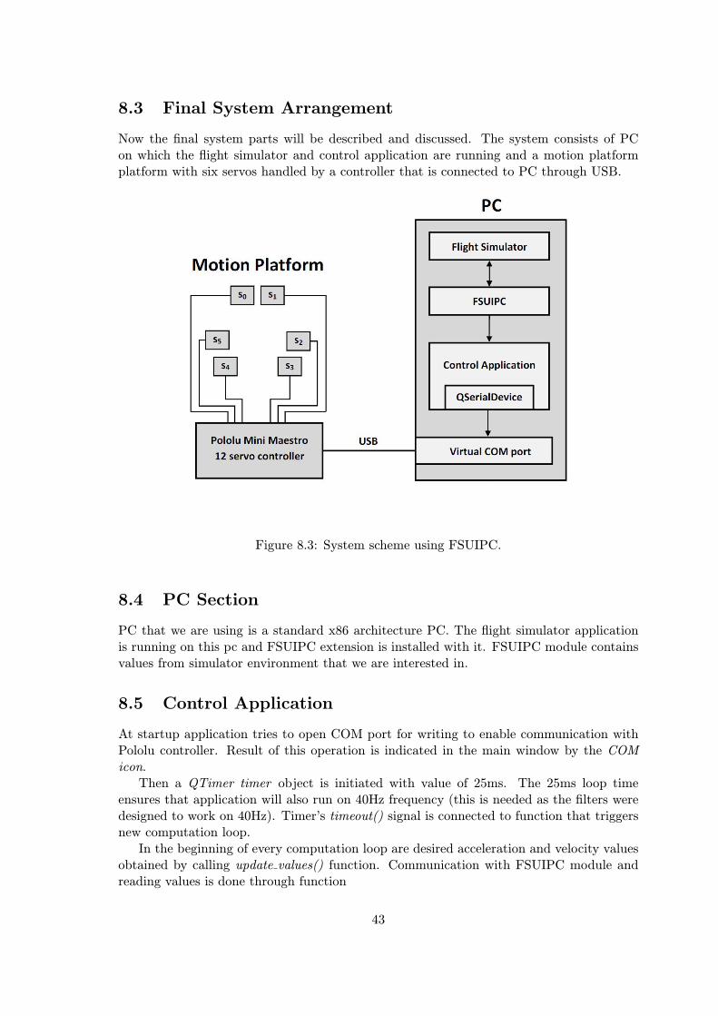
8.3 Final System Arrangement

Now the final system parts will be described and discussed. The system consists of PCon which the flight simulator and control application are running and a motion platformplatform with six servos handled by a controller that is connected to PC through USB.

Figure 8.3: System scheme using FSUIPC.

8.4 PC Section

PC that we are using is a standard x86 architecture PC. The flight simulator applicationis running on this pc and FSUIPC extension is installed with it. FSUIPC module containsvalues from simulator environment that we are interested in.

8.5 Control Application

At startup application tries to open COM port for writing to enable communication withPololu controller. Result of this operation is indicated in the main window by the COMicon.Then a QTimer timer object is initiated with value of 25ms. The 25ms loop time

ensures that application will also run on 40Hz frequency (this is needed as the filters weredesigned to work on 40Hz). Timer’s timeout() signal is connected to function that triggersnew computation loop.In the beginning of every computation loop are desired acceleration and velocity values

obtained by calling update values() function. Communication with FSUIPC module andreading values is done through function

43

bool FSUIPC Read(unsigned int dwOffset, unsigned int dwSize, void *pDest,unsigned int *pdwResult)

where dwOffset is offset of the value that we want to read (offset values can be foundin [17] ), dwSize is size of variable that we want to read and *pDest is a pointer to variableinto which the value will be stored. To check if the operation was succesfull *pdwResult ispointing on variable into which the state of reading will saved. After the reading of valuesis done, FSUIPC Process(unsigned int *pdwResult) function is called to finish the readingcycle.

8.5.1 Digital Filter Class

Then the data are scaled and passed to the filters. Every filter is an object of digital filterclass. This class is implemented according to Matlab’s 1–D digital filter [22] shown infig.8.6. Filter initiation is done by filling vector objects with a and b coefficients andtriggering init() method.

Figure 8.4: Matlab 1–D filter scheme[22].

Passing new input value to filter is implemented by functiondouble digital filter::next cycle(double in). Calling this function triggers new loop of dig-ital filter cycle and returns the output value. Output value can be also read by doubledigital filter::current value() function. Calling this function will not trigger a new loop ofdigital filter cycle.Filters are connected into a cascade of filters, one cascade for each channel (x,y and z

axis or pitch, roll and yaw). Each filter cascade contains high-pass or low-pass filter, in caseof high-frequency translation motions and angular motions followed by integrators.

8.5.2 Plots

The plots initiated at application startup inside the init plots() function. Title, x and yaxis description, y axis range and scale are set for every plot. Initiation of each plot isfinalized by update appearance() function. Plots are based on a Qwt plot class.Outputs of filters cascades and also input accelerations and angular velocities are shown

by plots in the control application window. These plots are:

• Body reference frame accelerations. Accelerations are displayed in m/s2 in rangefrom −5 to 5m/s2. Plot is displaying all three channels (x,y and z) each with its owncolor.

44

• High-pass filtered inertial frame accelerations. This plot is showing output of thehigh-pass filter. Range is from −1 to 1m/s2 as the amplitudes of high-pass filteredsignals are smaller.

• Simulator position. Here is shown the position of motion platform (double integratedaccelerations) separately for each axis.

• Low-pass filtered body accelerations – tilt channel. This plot displays output of low-pass filtered translational motions that are used for tilt channel coordination. Rangeis the same as with not filtered value as low-pass filtering is not lowering the amplitudeof low-frequency signals. Only values for x and y axis are shown as this technique isnot applicable to the accelerations along z axis.

• Body reference frame angular rates. Used units of velocities are degrees/s, and therange is from −20 to 20 degrees/s. Three channels are displayed within this plot (roll,pitch and yaw).

• High-pass filtered angular rates. Here are shown outputs of high-pass filters for eachof three channels. Plot range is smaller than with the previous plot – from −2 to 2degrees/s.

• Integrated angular rates. Data in this plot are outputs of integrators, the platformrotation angles.

All plots show data of the last 40 seconds of flight.

8.5.3 Communication with the Motion Platform

Then the outputs of the washout algorithm and the inverse kinematics of motion platformare computed and target position are loaded into buffer according to Pololu set multipletargets protocol. Buffer content is then send to COM port that is handled by QSerialDeviceclass. This COM port is only virtual as the platform is connected through USB.

8.5.4 AeroWorks Communication Protocol

Stewart platform control application is also able to gather the input data through AeroWorksprotocol. This protol is being used for communication with SimStar simulator located inFaculty of Information Technology on Brno University of Technology.Protocol functionality is implemented in netcom class and fsx class. Connection with

AeroWorks is initiated at control application startup. Desired host address and target portare set up, and also a mutex is created. Then a connection is tested by trying to getinput values for the first time. This is done by executing int GetData() function. If valuereturned by this function is equal to 0, communication is set up correctly. Accelerationand velocity values are stored inside the fsx object. From here they can be passed to thewashout algorithm as in the case of FSUIPC communication.

8.5.5 State Indicators

Control application window is equipped with three state indicators for providing informationabout current conditions of the simulation and the platform.

45

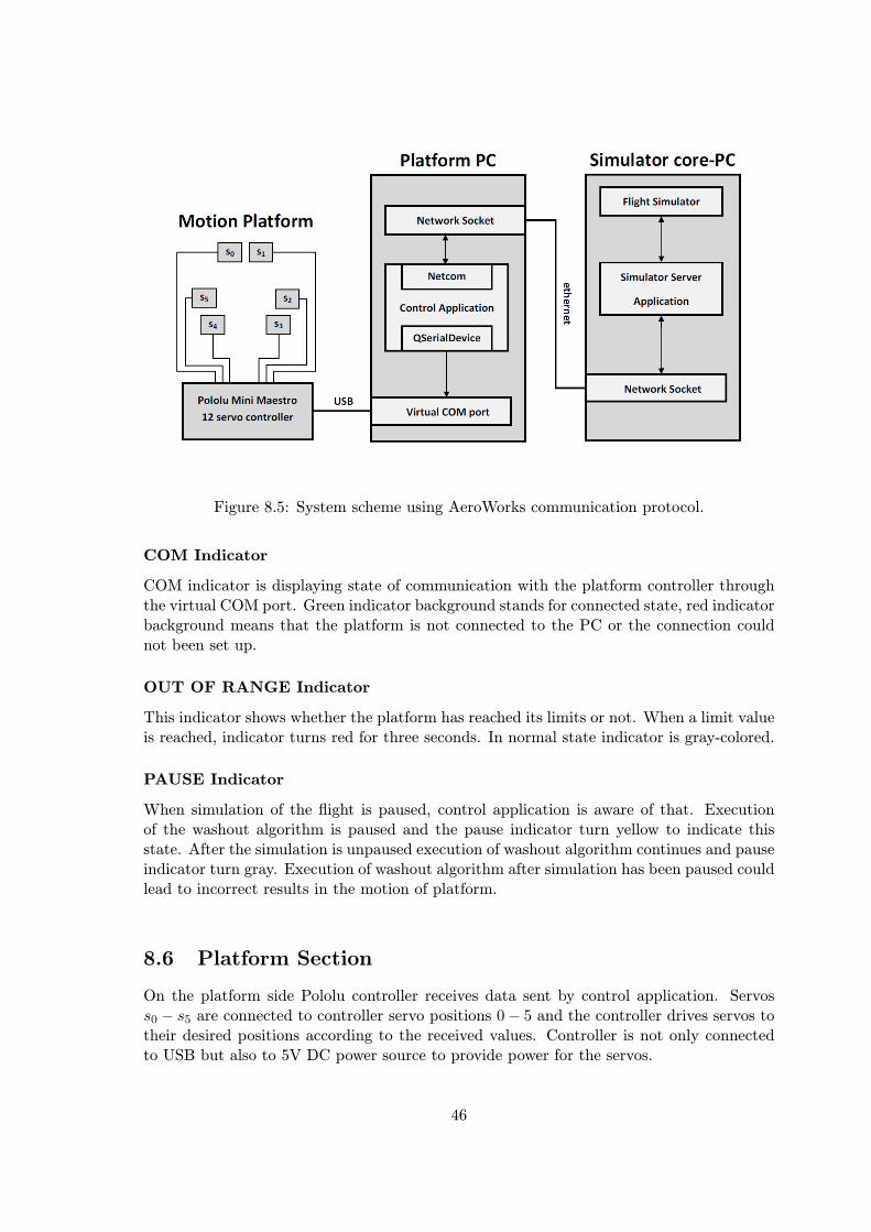
Figure 8.5: System scheme using AeroWorks communication protocol.

COM Indicator

COM indicator is displaying state of communication with the platform controller throughthe virtual COM port. Green indicator background stands for connected state, red indicatorbackground means that the platform is not connected to the PC or the connection couldnot been set up.

OUT OF RANGE Indicator

This indicator shows whether the platform has reached its limits or not. When a limit valueis reached, indicator turns red for three seconds. In normal state indicator is gray-colored.

PAUSE Indicator

When simulation of the flight is paused, control application is aware of that. Executionof the washout algorithm is paused and the pause indicator turn yellow to indicate thisstate. After the simulation is unpaused execution of washout algorithm continues and pauseindicator turn gray. Execution of washout algorithm after simulation has been paused couldlead to incorrect results in the motion of platform.

8.6 Platform Section

On the platform side Pololu controller receives data sent by control application. Servoss0 − s5 are connected to controller servo positions 0− 5 and the controller drives servos totheir desired positions according to the received values. Controller is not only connectedto USB but also to 5V DC power source to provide power for the servos.

46

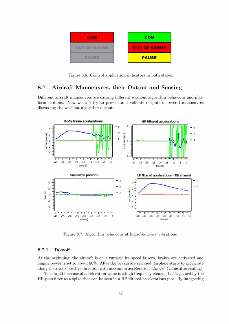
Figure 8.6: Control application indicators in both states.

8.7 Aircraft Manoeuvres, their Output and Sensing

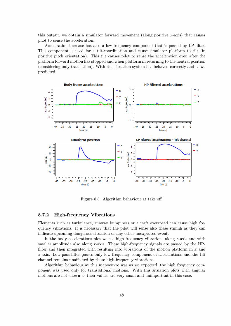
Different aircraft manoeuvres are causing different washout algorithm behaviour and plat-form motions. Now we will try to present and validate outputs of several manoeuvresdiscussing the washout algorithm outputs.

Figure 8.7: Algorithm behaviour at high-frequency vibrations.

8.7.1 Takeoff

At the beginning, the aircraft is on a runway, its speed is zero, brakes are activated andengine power is set to about 80%. After the brakes are released, airplane starts to acceleratealong the x-axis positive direction with maximum acceleration 4.5m/s2 (value after scaling).This rapid increase of acceleration value is a high frequency change that is passed by the

HP-pass filter as a spike that can be seen in a HP filtered accelerations plot. By integrating

47

this output, we obtain a simulator forward movement (along positive x-axis) that causespilot to sense the acceleration.Acceleration increase has also a low-frequency component that is passed by LP-filter.

This component is used for a tilt-coordination and cause simulator platform to tilt (inpositive pitch orientation). This tilt causes pilot to sense the acceleration even after theplatform forward motion has stopped and when platform in returning to the neutral position(considering only translation). With this situation system has behaved correctly and as wepredicted.

Figure 8.8: Algorithm behaviour at take off.

8.7.2 High-frequency Vibrations

Elements such as turbulence, runway bumpiness or aicraft overspeed can cause high fre-quency vibrations. It is necessary that the pilot will sense also these stimuli as they canindicate upcoming dangerous situation or any other unexpected event.In the body accelerations plot we see high frequency vibrations along z-axis and with

smaller amplitude also along x-axis. These high-frequency signals are passed by the HP-filter and then integrated with resulting into vibrations of the motion platform in x andz-axis. Low-pass filter passes only low frequency component of accelerations and the tiltchannel remains unaffected by these high-frequency vibrations.Algorithm behaviour at this manoeuvre was as we expected, the high frequency com-

ponent was used only for translational motions. With this situation plots with angularmotions are not shown as their values are very small and unimportant in this case.

48

8.7.3 Landing

Landing is one of the most critical manoeuvres performed with an aircraft. Practicinglanding is an important part of pilot’s training and sensing accelerations during landing iscrucial for plausible landing simulation.In the beginning, the aircraft is approaching the runway and small acceleration in z-axis

can be seen. When aircraft touches the runway, autobrakes are activated and noticeabledeceleration in shown as the plane is rapidly slowing down. Simulator translational motionwas appropriate in this case and also the tilt channel is showing the expected values.

Figure 8.9: Algorithm behaviour at landing.

8.7.4 Aircraft Roll Rotations

During the flight, the aircraft executes rotations along all three axes. These rotations arerequired to be sensed by pilot as they provide useful information about current aircraftmanoeuvres and its progress.What the system deals with are the angular rates, as they represent the change in the

aircraft rotation that we are interested in. As the range of the platform is quite limited,especially with the rotation, only the high-frequency component of the angular rates isbeing used.With this specific manoeuvre the aircraft is executing roll rotations (around x-axis

in body reference frame), at first in negative sense of rotation then stops rotating forapproximately 6 seconds after that followed by a roll rotation in positive sense. Output ofthe high-pass filter is showing spikes where the rotations have started and ended. In nextstage integrating these high-frequency components gives us the platform rotation. As we

49

can see, when the rotation starts the platform tilts in the same direction as the rotation togive the feeling that the aircraft rotation has started. After that the platform is returningto the neutral position until the end of the rotation comes (positive spike in HP filteroutput). By processing this component and tilting in the opposite sense as the endingrotation (positive in x-axis), platform signalizes that the aircraft rotation has ended. Thenthe whole maneuvre is being repeated but in opposite direction.In this situation, the provided stimuli were as we expected. High-pass filtering worked

correctly. Pilot would sense aircraft rotations in the right way and the platform would notreach its limits. Only plots displaying angular channel are shown with this manoeuvre.

Figure 8.10: Algorithm behaviour at roll rotations.

50

Chapter 9

Conclusion

Motion systems have proved to be an important part of a flight simulator. This thesisintroduced a view into history of motion systems and especially the Stewart platform.Formal background behind the inverse kinematics, aircraft motion in space and washoutalgorithm was presented as well.Application for the control of a 6DOF motion platform was implemented. It can op-

erate independently or in cooperation with AeroWorks SimStar simulator. Outputs of theapplications have shown to be valid.Further possible improvements are filter’s and scale coefficients fine tuning or platform

hardware upgrades. The real validation of provided stimuli would be possible with full sizemotion platform and experienced pilot who would review the motions.

51

Bibliography

[1] Federal aviation administration 14 cfr part 60. Federal Register Vol. 71, No. 209Monday, October 30, 2006 Rules and Regulations.

[2] Sunjoo Kan Advani. The Kinematic Design of Flight Simulator Motion-Bases. DelftUniversity Press, 1998. ISBN 90-407-1671-4.

[3] Joseph De Angelo. The link flight trainer.http://files.asme.org/asmeorg/Communities/History/Landmarks/5585.pdf,2000-06-10.

[4] Ilian Bonev. The true origins of parallel robots.http://www.parallemic.org/Reviews/Review007.html, 2003-01-24 [cit. 2011-12-1].

[5] Peter Chudy and Karol Rydlo. Intuitive flight display for light aircraft.AIAA-2011-6348, 2011.

[6] V. E. Gough and S. G. Whitehall. Universal tyre test machine. Proceedings of the9th International Technical Congress (FISITA ’62), 180:117–137, 1962.

[7] Prof. Dr. Florian Holzapfel. Flight performance lecture slides.

[8] T.S. Kelso. Orbital coordinate systems, part i.http://www.celestrak.com/columns/v02n01/, 2006-04-27.

[9] Lloyd D. Reid Meyer A. Nahon. Simulator motion-drive algorithms - a designer’sperspective. Journal of Guidance, Control, and Dynamics, 13:348–355, 1990.

[10] T.J. Monteodorisio, R.C. Brown, and W.B. Blake. Recommended Practice forAtmospheric and Space Flight Vehicle Coordinate Systems. American Institute ofAeronautics and Astronautics, 1992. R-004-1992.

[11] Ray L. Page. Brief history of flight simulation.

[12] K.H. Pittents and Podhorodeski. A family of stewart platform with optimaldexterity. Journal of Robotics Systems, 10:463–479, 1993.

[13] Brian L. Stevens and Frank L. Lewis. Aircraft Control and Simulation. John Wiley &sons, Inc., 2003. ISBN 0-471-37145-9.

[14] D. Stewart. A platform with six degrees of freedom. Proceedings of the Institution ofMechanical Engineers 1965-1966, 180:371–386.

[15] WWW pages. Acme worldwide enterprises inc. http://www.acme-worldwide.com.

52

[16] WWW pages. Aeroworks. http://merlin.fit.vutbr.cz/AeroWorks/.

[17] WWW pages. Fsuipc. http://www.schiratti.com/dowson.html.

[18] WWW pages. Handbook of aeronautical knowledge.http://www.aboutflight.com/handbook-of-aeronautical-knowledge/

ch-02-aircraft-structure/chapter-summary.

[19] WWW pages. Heli trainer.http://www.heli-aviation.de/en/technology/heli-trainer/.

[20] WWW pages. Human neurophysiology.http://www.humanneurophysiology.com/vestibularsystem.htm.

[21] WWW pages. Mathworks - matlab.http://www.mathworks.com/products/matlab/.

[22] WWW pages. Matlab r2012a documentation – filter.http://www.mathworks.com/help/techdoc/ref/filter.html.

[23] WWW pages. Pololu robotics and electronics. http://www.pololu.com/.

[24] WWW pages. Qt reference documentation. http://doc.trolltech.com/4.5/.

[25] WWW pages. Qwt - qt widgets for technical applications.http://qwt.sourceforge.net.

[26] WWW pages. Variable stability flight simulator.http://s6.aeromech.usyd.edu.au/vsfs/sim history.html.

[27] WWW pages. Virtual aircraft museum.http://http://www.aviastar.org/air/sweden/saab gripen.php.

[28] WWW pages. What when how.http://what-when-how.com/gps-with-high-rate-sensors/ecef-coordinate-systems-gps/.

[29] WWW pages. Which filters are noisier analog or digital?http://www.analog-europe.com/en/which-filters-are-noisier-analog-

or-digital-part-2.html?cmp id=71&news id=222902322.

[30] WWW pages. Histology / cell biology thread.http://www.med-ed.virginia.edu/courses/cell/, 2011.

53

Appendix A

CD Contents

Enclosed CD contains stewart platform control application source files, binary executablefile of this application, Matlab demonstration application source files, this thesis LATEX sourcefiles and a pdf version of this thesis.

54

Appendix B

Control Application Screenshot