WITH A BANG, NOT A WHIMPER:

PRICKING GERMANY'S "STOCKMARKET BUBBLE" IN 1927

AND THE SLIDE INTO DEPRESSION

Hans-Joachim Voth*

ABSTRACT

Asset price inflation presents central banks with a puzzle. We examine thecase of Germany, 1925-7, when the Reichsbank intervened to bring down thestock prices, rectify imbalances, and curb speculation. The evidence stronglysuggests that the German central bank under Hjalmar Schacht was wrong tobe concerned about stockprices – no bubble can be discerned. Moreover, themisguided intervention had important real effects that helped to tip Germany– then the world's second-largest economy – into depression.

JEL classification codes E31, E43, E44, N14, N24Keywords Stockmarket, Asset Prices, Bubbles, Germany, Monetary

Policy.

* Centre for History and Economics, Cambridge CB2 1ST, UK and Economics Department, UniversitatPompeu Fabra, 08005 Barcelona, Spain.

2

Should asset bubbles be pricked? Recent experience suggests that the risks involved can be

substantial. In the US in 1929, as well as in Japan in 1989, it was intervention by the central

bank that eventually brought rapid increases in the valuation of stocks and other assets to an

end. Interest rates were raised when concerns about asset inflation spilling over into the

economy at large became pressing; sooner or later, equity valuations slumped. The extent to

which the Japanese and American market were overvalued at the time of central bank

intervention is controversial. What is clear is that deflating what the central banks saw as asset

bubbles entailed substantial costs for the economy at large. Today's policy debate again

centres on the importance of increases in stock prices at a time when inflation remains

subdued. Instead of intervening directly, the Chairman of the Federal Reserve, Alan

Greenspan, decided to "talk the market down" by emphasizing the dangers of what he saw as

"irrational exuberance". His comments came when the Dow was at 6,500 points. As of

November 1999, it had risen a further 65 percent.1

This paper examines one of the most important historical episodes "when the music

stopped". In early 1927, the Reichsbank's flamboyant president, Hjalmar Schacht, began to

believe that funds were being diverted from "productive uses" to the stockmarket. Also, he

feared that the Reichsbank's holdings of gold and foreign exchange could suffer if the

substantial gains of foreign investors were repatriated. Instead of increasing interest rates, he

decided to lean on the banks to reduce their lending against shares held as collateral. To add

emphasis to his policy, banks that failed to comply were threatened with reduced (or even no)

rediscount facilities. Banks were highly vulnerable to this kind of threat as the liquidity of their

balance sheets was not high.2 On May 12, the Berlin banks issued a joint statement in which

they described far-reaching measures to curtail lending against securities. The next day

became known as "Black Friday" – prices retreated on a broad front, falling by an average of

11%. The impact was felt most severely in the futures market, and then spread to the cash

market. Within one month, shares had lost one quarter of their previous value. At the same

time that prices were falling, turnover also collapsed. Between the second and the third

quarter of 1927, revenue from stamp duty, a direct measure of stockmarket turnover, fell by

more than 50 percent.3

1 Krugman 1999.2 Balderston 1993, p. 207-8.3 Konjunkturstatistisches Handbuch 1936, p. 115.

3

A BUBBLE?

The market's rebound between December 1925 and April 1927 was spectacular indeed – an

increase of 163.8% in real terms over a period of 17 months. But a rapid increase in the index

alone is clearly insufficient to support the claim that there was a bubble in the German stock

market. Hamilton and Whiteman have argued the existence of a bubble is hard to prove

conclusively – test results may simply be driven by an inappropriately-specified model.4 In

testing for the existence of a bubble, we can either compare valuations with some indicator of

'fundamental' value, or we can examine the time-series properties of the data. There are three

pieces of evidence that imply that there was no systematic overvaluation in the German

stockmarket prior to the Reichsbank's intervention. First, valuations of stocks by any

conventional measure do not appear very high. Second, the rebound of German stock

markets is typical of other "re-emerging markets". Finally, there is no time-series evidence for

an asset bubble.

400

600

800

1000

1200

1400

1600 3

4

5

6

7

8

1925 1926 1927 1928 1929

Intervention

Dividend Yield

Stock Price Index

Dividend Yield and Stock Prices in Germany, 1925-30

Figure 1

4 Hamilton 1987, Hamilton and Whiteman 1985.

4

A simple valuation measure is the dividend yield, defined as the ratio of dividends to the stock

price.5 Figure 1 shows the long-term development of the dividend yield (in percentage points)

and the market index. The dividend yield over the period 1926/ early 1927 declined sharply.

During the period 1925-12 to 1927-4, it averaged a mere 3.8%. The lowest value of 3.1% was

reached in January 1927. By contrast, the historic long-term average (1870-1913) was 5.4%.

Nonetheless, prices relative to dividends were not unprecedently high – over the years 1920-

24, the dividend yield had repeatedly dipped below 4%. The lowest value recorded during the

period 1870-1927 was seen in February 1924, when the dividend yield stood at 1.3% – more

than two thirds below the average value during the so-called bubble period.

0

2

4

6

8

100

500

1000

1500

70 75 80 85 90 95 00 05 10 15 20 25

Dividend Yield and Stock Market Index, 1870-1927

stockprice index (100=1870)

divi

dend

yie

ld (

in %

)

dividend yield

stockprice index

Figure 2

Figure 2 examines the reasons for the decline in the dividend yield more closely. The

turnaround in prices preceded that in dividends by approximately six months. The runup in

share prices nonetheless appears justified by the magnitude of gains in dividends paid.

5 The data is from Gielen 1994, and was kindly made available in electronic form by George Bittlingmayer.

5

400

600

800

1000

1200

1400

1600

30

40

50

60

70

80

1925 1926 1927 1928 1929

Stock Price and Dividends, 1925-1930

stockprice index

dividends

stoc

kpric

e in

dex

(187

0=10

0)

dividends

Figure 3

Investing in an equity with a dividend yield below the rate of return on riskless assets will be

rational if investors anticipate (sufficiently large) price increases in the future. Ultimately, these

must be underpinned by the company's ability to generate cash. The extent to which future

dividend increases should be discounted depends on the appropriate interest rate.

Gordon presents a model to calculate the implied dividend growth.6 In the simplest case,

with constant dividend payments, the price of a share should simply be equivalent to the

discounted value of future dividend payments:

where P is the price of a share, D is the dividend payment, R is the discount rate, and N is the

number of years for which the firm is expected to survive.7 If dividends grow at g % p.a., then

the calculation simplifies to

6 Gordon 1962.7 Note that the discounted value of the firm in its final year is set to zero.

( )P

D

R tt

N

=+=

∑11

6

Since D0 and P are observed, we can calculate the implied growth rate of dividends subject to

R:

The difficulty is now in chosing the appropriate rate at which future dividends should be

discounted. The following figure gives implied rates of dividend growth for German shares for

three alternative values of R – the monthly interest rate plus a risk premium of 3%, the

interest rate on mortgage bonds with a gold clause, and an assumed rate of return of 10%.8

Figure 4

8 A risk premium of 3 percent appears to be an upper bound on the appropriate rate – the long term real returnon German equity (over the period 1924-1991) was 1.91 percent. Cf. Jorion and Goetzmann (1999), table 1, p.964.

PD g

R g=

+−

0 1( )

gPR DD P

=−+

7

The implied rates of dividend growth derived from the interest rate market are essentially flat

over the period. Using the return on goldbonds plus the three percent risk premium, the

implied growth rate rises to six percent in the later months of 1926. It then falls during most of

the bull-run, and stands at less than 4.5% before the Reichsbank intervened. The implied

divident growth rates from monthly interest rates are consistently higher, but show a broadly

similar pattern over time. When we use a constant discount rate of 10%, however, the implied

dividend growth rate increases from approximately 2% to over 6% in the final phase of the

bull run, only to settle down to below 5% in the final months of 1928.

Before World War I, the implied rate of dividend growth was 1.81% (1870-1913).9 This

seems to suggest that the German market was indeed beginning to look overvalued by the

standard of Imperial Germany when the Reichsbank under Schacht decided to strike. Yet

how unrealistic was an increase in dividends at an annual rate of 4.6%? Before WWI,

dividends had grown at a rate of 4.5% p.a.10 Investors were therefore only betting on a rate of

dividend growth that would have been a touch higher than during the pre-war era. More

importantly, Weimar Germany's economy delivered dividend growth that outstripped

expectations implicit in the Gordon model, and higher than those accomplished before WWI.

In the years after the intervention to prick the "bubble", and into the first year of the Great

depression, dividends continued to grow at a healthy rate of 6.3% (4/ 1927-12/ 1930). Not

even the constant discount rate of 10%, nor the monthly interest rate plus a 3% premium,

gives implicit rates of dividend growth that are significantly higher than this. The sharp fall in

dividends seen in 1931/ 32 was arguably driven by the unique nature of the Great Slump, and

was not a result of a cyclical downturn that rational investors could have anticipated in

1926/ 27.11

The three alternative discount rates shown in Figure 4 show significantly different trends

over time. The reason for this divergence is that interest rates came down sharply. Monthly

interest rates fell from 11.92% in February of 1925 to 5.77% in June 1926. The yield on

mortgage bonds with gold clauses declined from 8.81% in November 1925 to 6.07% in

February of 1927. That equity prices should react so strongly to changes in interest rates is no

surprise – Shiller's seminal contribution in 1982 has sparked a whole literature demonstrating

9 The rate for the period 1910-13 is almost identical.10 The real rate of increase was 4.08%.11 The extent to which Weimar's economy was already doomed in the second half of the 1920s has been hotlydiscussed by Borchardt (1991), Holtfrerich (1990), Ritschl (1997), and Voth (1995). Balderston (1982) provides

8

that most of the variation in stock prices cannot be explained by subsequent changes in

dividends.12 Instead, it is changes in the discount factor that appear to be driving much of the

variance. Therefore, if there is anything unusual about Weimar's only stockmarket boom, it is

the extent to which dividend increases justified the run-up in prices. During the period when a

bubble was allegedly developing, the average implied rate was 4.6% (using the gold bond

interest rate as the benchmark), or on the same level as in 1925.13 For all the spectacular rise in

prices, implied dividend growth was largely unchanged because the very high interest rates

after the stabilization of the Mark gradually came down. This suggests that the increase in

prices was underpinned by a "normalization" of the fundamentals, and not herd behaviour.

We should therefore note that the relatively low implicit rates of dividend growth are partly a

result of lower interest rates – themselves driven by the Reichsbank's aggressive loosening of

monetary policy which brought the discount rate down from 10 percent in 1925 to 5 percent

in 1927. In other words, it may still be the case that equity valuations were too high by some

standard other than those of the Gordon model; but to say so is to claim that interest rates

were inappropriately low. This would cast a different light on Reichsbank policy, which would

have been as much responsible for creating a bubble as it was for pricking it.

As the German economy emerged out of the mini-slump in 1926, there were good

reasons to believe that both prices and dividends would continue to rise in the near future.

Even during the "bubble" months, share prices were down 59.5% from their 1913 level.

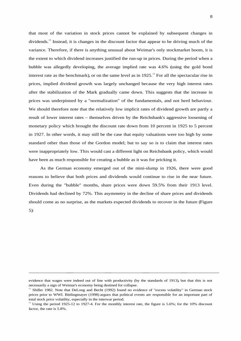
Dividends had declined by 72%. This asymmetry in the decline of share prices and dividends

should come as no surprise, as the markets expected dividends to recover in the future (Figure

5):

evidence that wages were indeed out of line with productivity (by the standards of 1913), but that this is notnecessarily a sign of Weimar's economy being destined for collapse.12 Shiller 1982. Note that DeLong and Becht (1992) found no evidence of "excess volatility" in German stockprices prior to WWI. Bittlingmayer (1998) argues that political events are responsible for an important part oftotal stock price volatility, especially in the interwar period.13 Using the period 1925-12 to 1927-4. For the monthly interest rate, the figure is 5.6%; for the 10% discountfactor, the rate is 5.8%.

9

Determinants of Dividend Yield

Change in Dividend Yield, 1913-25/27

5.5

3.82.2

-3.9

Dividend Yield1913

Reduction inDividend

Fall in StockPrice

DividendYield 12/25-

4/97

Figure 5

As rapid subsequent dividend growth makes clear, investors were correct in thinking that

fundamentals would eventually recover. By paying a higher price for stocks in terms of the

current dividend yield, their behaviour implicitly assumes that dividends would not

permanently remain depressed by almost 60%. By 1927, according to Maddison, real

German GDP per capita was already 10.5% higher than in 1913.14 Even if wages had risen

more than output prices and labour productivity, thus pushing up unit labour cost, it hard to

see that expecting dividend growth of 4.6% was a sign of "irrational exuberance". At such a

rate of growth, it would have taken German firms another 28 years – until 1954 – to pay the

same total dividend as the one distributed in 1913.15 In an economy that had in some ways

returned to 1913 levels of output, this is clearly too pessimistic. That investors failed to profit

from their prudent judgements during the boom is mainly a result of the Reichsbank's

intervention.

Standard valuation measures such as the dividend yield do not suggest that the German

equity market was rapidly becoming overvalued in 1926 and early 1927. Diba and Grossman

argue that, in the case of a rational bubble, first differences of share prices will be non-

14 Maddison 1995. The stock price index does not adjust for those firms listed in 1913 who were now located onthe territory of a foreign state. Total German GDP in 1926 was 2.3% below the 1913 value (using post-1918territory). Note that Ritschl (1997) has recently presented detailed evidence suggesting that Maddison's estimates(based on Hoffmann's (1965) data) may be too optimistic.15 Calculated in real terms.

10

stationary.16 For the period when 'bubble trouble' was allegedly building rapidly, we can

clearly reject the null hypothesis of non-stationarity (Table 1).17

Table 1: Unit Root Tests – Stock Market Returns

sample period 1925:12-1927:04 1926:01-1927:04 1926:02-1927:04 1925:12-1927:05

ADF -4.4** -6.04** -4.3** -3.7*

PP -5.1** -5.3** -4.5** -4.3**

DW 2.4 2.2 2.2 2.1

** indicates significance at the 1% level* indicates significance at the 5% level

An alternative approach is to examine the time-series properties of stock prices. Shiller and

Campbell suggest to test if stock prices and dividends are I(1) and cointegrated; if they are,

there is little reason to suspect that there is a bubble building up.18 The Johansen test allows us

to test for the number of cointegrating vectors. If there is one cointegrating vector for two

variables, then they are cointegrated. If there the null of no vector cannot be rejected, or there

are as many vectors as there are variables, then there is no evidence of cointegration. Table 2

gives the results for using the Johansen procedure for the dividend and and stock price series.19

16 Diba and Grossman 1988.17 For the Philipps-Perron test, I used the Newey-West truncation at 2 lags.18 Campbell and Shiller 1987. Rappoport and White (1993) apply this procedure to the American stockmarket in1929, and find no evidence of a bubble based on this test. Note, however, that they find that their bubble term –derived from a model of the brokers' loan market – also is cointegrated with dividends and stock prices.19 Pretesting showed conclusively that there was no trend in the data; we also assumed no trend in the datagenerating process. Objections might be raised because we use cointegration techniques on a relatively briefperiod. Note, however, that recent work by Choi and Chung (1995) and Hooker (1992) suggests that higherfrequency may compensate for reductions in sample length.

11

Table 2: Johansen Test for Cointegration – Dividends and Stock Price

Eigenvalue Likelihoodratio

5% criticalvalue

1% criticalvalue

Hypothesis: Noof co vectors

1/ 1925-9/ 1935 0.132 18.3 12.53 16.31 0*

0.000003 0.0036 3.84 6.51 1

1/ 1925-12/ 1929 0.28 19.75 12.53 16.31 0*

0.002 0.17 3.84 6.51 1

1/ 1925-12/ 1928 0.38 23.3 12.53 16.31 0*

0.005 0.24 3.84 6.51 1

Note: * indicates significance at the 5% level

For most sample periods covering the "bubble", there is clear evidence from the Johansen

cointegration test that dividends and stock prices are cointegrated – and that there is therefore

no reason to suspect that rapid price increases were fundamentally irrational. However, if we

restrict the sample period to the brief period when price increases were most rapid – January

1926 to April 1927 – the cointegrating relationship between stock prices and dividends is no

longer apparent in the data.20 Simple estimation of cointegrating vectors using two variables

ignores the fundamental importance of the discount factor, as demonstrated by Shiller. If we

include the interest rate on mortgage-backed bonds in our estimation procedure, the results

clearly indicate the presence of one cointegrating vector.21 This suggests that some of the

market's rapid rise in 1926-7 may have been more to do with equities become more attractive

vis-à-vis bonds than with a simple, dividend-driven boom.

The time-series properties of the dividend yield have also been used as a test for

existence of bubbles in stockmarkets.22 A unit root in the price-dividend ratio violates the no-

bubble assumption. Testing for unit roots in the price-dividend ratio during the bubble period

– January 1926 to April 1927 – using both the augmented Dickey-Fuller and the Phillips-

Perron technique allows us to reject the null of non-stationarity.23 This suggests that our failure

to find cointegration between dividends and stock prices during the 'bubble' period may be a

result of the low power of the tests in a restricted sample.

20 The Johansen test rejects the presence of a maximum of only one integrating vectors, i.e. no cointegrationeither.21 We reject the hypothesis of no cointegrating vector at with a likelhood ratio statistic of 49.3 (95% criticalvalue=34.9), but cannot reject the presence of at most one vector (18.6 vs. a 95% critical value of 19.96).22 Craine 1993.23 The PP statistic is –5.6 vs. a 1% critical value of –3.9, whereas the ADF statistic is –5.2 vs. a 1% critical value of–3.9.

12

Clearly, an economy recovering from hyperinflation is in an unusual situation. So is its

stockmarket. Poor stock returns during inflationary periods have been observed in almost all

countries.24 Once countries stabilize, their markets "re-emerge". Unusually high returns are

often associated with this return to normalcy. Table 3 gives descriptive statistics for twenty-

two emerging markets after "emergence", and compares these figures with the results for

Germany during Weimar's only boom.25

Table 3: Monthly returns (in %) and volatility22 're-emerging'

marketsGermany

36 monthsaverage 3.24 2.85std.dev. 0.54 0.09

48 monthsaverage 3.13 2.17std.dev. 0.45 0.08

60 monthsaverage 2.64 1.62std.dev. 0.41 0.07

Note: Observation period in the German case beginning 7/ 1924.

The observation period in the German case was chosen so as to maximize the return, thus

biasing the comparison against finding unspectacular returns in the German stockmarket. For

all observation windows, a starting date of July 24 was found to serve the purpose. In this way,

we are biasing our results in favour of finding dangerously and "exuberantly" rapid equity

price appreciation in post-inflationary Germany. Nonetheless, German monthly returns are

markedly below the average observed in other countries that saw a period of normalization in

their stockmarkets. Volatility in the German case is lower. The longer the time period

considered, the clearer the relative underperformance of the German market. Again, judged

against the background of other stockmarkets recovering from similar blows, the German

market was not behaving unreasonably exuberant.

Finally, we can examine the macroeconomic environment. Bubbles do not accidentally

descend on economies developing normally; a number of authors have argued that they are

24 Fama and Schwert (1977), Beaulieu (1995).25 The information in column 1, table 2 is from Goetzmann and Jorion (1996).

13

systematically related to other imbalances in the economy.26 A number of past episodes

suggests that five main variables can be examined. The majority of bubbles in the past has

been associated with unusually high growth, unusually low inflation, a rapid rise in the money

supply, a deterioration of the current account as well as falling savings rates. On the bubble

checklist compiled by King, the canonical cases score highly – the Japanese and UK bubbles

of the late 1980s, Mexico in the early 1990s, and the current US. Germany in the 1920s, in

contrast, shows few of the familiar signs of a bubble building up. Growth of close to ten

percent in 1927 is the only feature of the macroeconomic picture that fully fits the bill.

Inflation is below trend, but rising relatively quickly towards the end of the period – not a

perfect parallel with the unusual degree of stability seen in the US or Japan. On all other

scores, interwar Germany does not show the normal signs of an economy heading towards

excessive asset inflation.

THE CONSEQUENCES OF THE CRASH – SHARE PRICES, TOBIN'S Q AND THE SLIDE INTO

DEPRESSION

The preceding section established that there was little reason for Schacht's attempt to bring

down the equity market. The next question we need to address is if the central-bank's

intervention and the turmoil it induced in the asset markets had any real effects. Some

contemporaries claimed that the Reichsbank's intervention wreaked havoc in the economy.27

The literature's view is also controversial. While Hardach maintains that the crash had severe

consequences, Ritschl has argued that it was of little consequence.28 Balderston concluded that

weakness in both the bond and the equity market were responsible for the early start of the

depression in Germany.29 We find that the slump in equity prices had important real effects,

and that investment was lower than it would have been otherwise, had it not been for the

intervention by the Reichsbank.

In the case of the US depression after the crash of 1929, analysis of the transmission

mechanism has focused on declines in consumption. A fall in business activity as a direct result

of the crash was not being anticipated by contemporaries.30 Also, wealth effects – reductions in

26 King 1999.27 Weber 1928.28 Hardach 1976, Ritschl 1997, p. 88-90. Ritschl 1999, p. 4 argues for a larger impact on machinery investment.29 Balderston 1983.30 Dominguez et al. 1988.

14

consumer spending as a result of lower net household wealth – appear to have been very

small. However, it may have served to make households illiquid, and uncertainty over future

income may have caused a reduction in expenditure on consumer durables.31 In Germany,

consumer spending continued to rise for a full year after the crash. Even then, it does not

collapse, but remains fairly constant until the onset of the Great Depression. What the crash

did influence was investment activity – the single most important determinant of variations in

GDP during the late 1920s.32

Typically, empirical studies show only a weak connection between investment and Q

(either marginal or average).33 Barro's work on the US in the 1920s and 1980s, however,

demonstrates that stock prices themselves are better predictors of investment and output than

Tobin's Q. The calculated equity component of Q turns out to be a poor proxy for stock

prices.34 Using stock prices, Barro finds that the collapse in share prices in 1929 can explain a

significant part of the decline in US investment, 1930-32. Earlier work on modelling

investment in interwar Germany has already addressed the issue of Tobin's Q and its

predictive value for capital formation. Ritschl argues that investment reacted extremely

sensitively to changes in pseudo-Q.35

31 Mishkin 1978, Romer 1990.32 Temin 1971, Temin 1976, p. 149-60.33 Summers 1981.34 Barro 1990, p. 549.35 Ritschl 1994.

15

400

600

800

1000

1200

1400

1600

-2000

0

2000

4000

6000

8000

10000

25 26 27 28 29 30 31 32 33 34 35

Stock Prices and Investment, 1925-39

stock price index

net investment

Figure 6

Figure 6 compares aggregate investment with the level of stock prices in Germany, 1925-

1935. Both series track each other closely. The sharp run-up in equity prices precedes the

turning point of the investment series. Also the downward turning point is reached just a few

months after the Reichsbank's intervention. Some brief episodes apart, both series begin their

long decline in 1927, after Schacht's intervention. It is only after the stock market index has

bottomed out in 1932, and after it began its recovery, that investment turns upwards.

Granger-causality tests also clearly demonstrate that equity valuations mattered for investment

– for the period 1/ 1925 to 9/ 1935, the standard F-test gives a statistic of 6.2, equivalent to a

probability of 2.5 percent that we cannot reject the null of no granger causality running from

stock prices to investment. The reverse, testing for investment causing stock prices, yields a

statistic of 0.24, equivalent to a 78% probability.

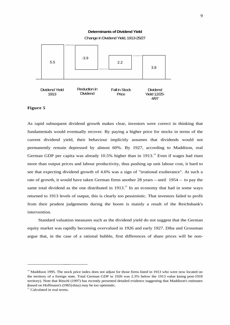
We repeat Ritschl's estimation for the period at hand, again employing the Johansen

technique. Following Barro, we use stockprices directly. For the late 1920s, there is consistent

evidence that stock prices and investment in Weimar's economy are cointegrated (Table 4).36

36 Pretesting established that the data series are not trended; also, we assumed no trend in the data generatingprocess.

16

Table 4: Johansen Test for Cointegration – Investment and Stock Price Index

Eigenvalue Likelihoodratio

5% criticalvalue

1% criticalvalue

Hypothesis: Noof co vectors

1/ 1925-9/ 1935 0.02 2.54 12.5 16.3 0

0.0001 0.014 3.84 6.5 1

1/ 1925-12/ 1929 0.247 16.5 12.5 16.3 0*

0.000005 0.00299 3.84 6.5 1

1/ 1925-12/ 1928 0.32 18.2 12.5 16.3 0*

0.13 0.62 3.84 6.5 1

It is only when the sample period is extended beyond the onset of the Great Depression that

this relationship begins to fall apart. For the period as a whole, investment and stock price

track each other quite closely, and the run-up in prices in 1926/ 27 appears more like a

correction of a prior undervaluation than a period of irrational exuberance. The sharp

correction induced by the curtailment of lombard credit therefore caused investment spending

to be lower than it otherwise would have been.

How important was this correction in economic terms? Using the values from the

estimated cointegrating vector, we can calculate a counterfactual investment performance had

Schacht abstained from his pre-emptive strike. If stock prices had carried on rising at a

moderate rate of two percent p.a., then they would have been some 12 percent higher than

their actual values at the end of 1928. Investment would have been some 14 percent higher.

At the end of 1929, the 'penalty' had widened to 28 percent. Our results thus serve to

reinforce Balderston's argument that the early downturn in Germany after 1927 owed much

to government intervention in asset markets.37

Of course, there is no particular reason to assume that stock prices should have risen at

a rate of 2 percent. As our preceding analysis suggested, a dividend growth rate of 4.6 percent

is what the market expected while the "bubble" was allegedly developing. What the economy

delivered was dividend growth of more than 6 percent p.a.38 Assuming that share prices could

have carried on rising at the rate of dividend growth implies that investment at the end of

1928 would have been 23 percent higher; by the end of 1929, the difference between

37 Balderston 1983, 19938 Some authors have voiced doubts about the viability of dividend increases in the Weimar period – they claimthat dividend growth was not always fully underpinned by profits. This, in itself, is not unusal; year-to-yearchanges in profits are rarely reflected in dividends. A fundamental divergence of the long-term growth rate ofprofits and dividends would be a different matter, but there is no conclusive evidence that would support such aclaim.

17

counterfactual and actual levels grows to 39 percent.39 Much of the "investment shortfall" that

some authors have claimed to have found in interwar Germany may, if it did exist, be the

result of the central bank's attempt to force down stock prices.40

Before we conclude that the negative consequences of Schacht's intervention were grave

and unnecessary, we need to address the reasons why the President of the Reichsbank

intervened. High stock prices appeared to indicate that Germany had recovered from the war,

a signal that Schacht, a vociferous opponent of reparations, was not keen to send.41 He also

feared that the stability of the banking system would suffer if banks were lending too

generously against securities. Also, price pressures were becoming more obvious in the

German economy as the year 1927 wore on. The CPI, which stood at 137.9 in January 1925,

was 2.6 percent higher by the beginning of 1926. By January 1927, it had risen by 5.3 percent

in total over the preceding two years. The mild deflation of 1926 had turned to gradual

inflation. Year-on-year, the rate of price increases began to accelerate. In January 1927,

annualized inflation was 2.6 percent; in February, it was to 3.8 percent, rising to 4.1 percent

in March. In May, when Schacht decided to strike, the annualized rate was still above 4

percent. A later report by the Reichsbank was making familiar points about "wealth effects",

additional purchases of consumer goods as a result of higher net worth. In an economy

impoverished by war and inflation, such a spending spree – the Reichsbank argued – would

have been more probable. Nonetheless, because of the dangers involved, it was imperative to

end excessive speculation.42

39 Disaggregated analysis supports this view – Ritschl (1999) shows that the downturn in domestic Germanmachinery orders coincided exactly with the turning point in the stock market.40 Spoerer (1997) presents conclusive evidence that investment in interwar Germany was not lower than duringthe Empire. Cf. also Voth 1993. For a view to the contrary, Borchardt 1991.41 Beer 1998, p. 201.42 Beer 1998, p. 206.

18

136

140

144

148

152

156

400

600

800

1000

1200

1400

1600

25:01 25:07 26:01 26:07 27:01 27:07 28:01 28:07

CPI

stock price index

Stock Prices and the Consumer Price Index, 1925-28C

PI (

100=

1913

)

stockprice index (100=1870)

Figure 7

That Schacht may have been right in worrying about inflationary pressures does not

necessarily lead to the conclusion that throttling the stock market was a wise policy decision.

Figure 7 plots the consumer price index side-by-side with the stock price index. It is true that

during the stockmarket boom, prices were rising. Yet the overall degree of co-movement is

only remarkably for being so small. The sharp decline in prices in 1926 is not mirrored in

stock prices, and the bust in 1927 only appears to do very little to slow down price pressure in

the economy.

The cause of accelerating price increases is not difficult to find. The Reichsbank had

lowered the discount rate from 10 percent in 1925 to 5 percent in 1927. Only in May 1927

did it increase the rate to 6 percent. A simple test of how loose central bank policy was

contrasts these rates with the ones implied by the Taylor rule.43 The interest rate is set

according to

r gy h r f= + + − +π π π( *)

where r is the central bank's interest rate, π is the inflation rate, y is the percentage deviation

of real output from trend, π-π* is the difference between actual inflation and the desired level

19

π*, rf is the target real interest rate, and g and h are policy variables. A standard Taylor rule

uses π*=2, g=h=0.5, rf=2.44

To derive the appropriate rates for interwar Germany, we need to assess the size of the

output gap. German output was, on some measures, below its pre-war trend. At the same

time, it is not clear that Germany could have easily returned to the pre-war growth path,

given the changes in the structure of international trade and supply shocks such as reductions

in the length of the working week. We do not need to make an explicit decision on this point if

we simply ask – how high would the output gap have to be to justify a rate as low as five

percent? The Taylor rule implies that the German economy would have had to be a full four

percentage points below its productive potential to justify the Reichsbank's discount policy. An

output gap of 2 percent would have suggested a rate of 6 percent; a gap of 0 one of 7 percent.

Given that employment and investment were rising rapidly at the time, it is difficult to argue

that there was still slack on a scale sufficient to explain the Reichsbank's loose monetary

policy. The story is then one of excessive monetary easing by the central bank in the aftermath

of the "mini-slump" of 1926, driving up both domestic demand and, via a lowering of interest

rates, the stock market. The crackdown on "speculation" is therefore equivalent to shooting

the messenger, bearing news of one's own flawed policy.

43 For an overview of rules for targeting inflation, cf. Bernanke, Laubach, Mishkin, and Posen 1999.44 Taylor 1993.

20

CONCLUSION: A "SOFT LANDING" GONE WRONG

Rapid increases in asset prices present the central bank with a dilemma. If there is a danger of

price increases spilling over into the rest of the economy, it may appear sensible to "step on

the brakes" and deflate what appears to be a bubble. At the same time, active intervention in

asset markets, and deliberate attempts to change prices, may be as dangerous as other forms

of tinkering with the price mechanism. Distortions in relative prices may cause misallocation

of resources, and perhaps more importantly, growth and investment can suffer if the central

bank decides to intervene at an inappropriate time. Simulation studies of monetary policy

regularly find that an explicit targeting of asset prices – over and above their effect on the

price level – may amplify "boom-bust" cycles.45

This paper has analysed the stockmarket bust of 1927, when the Reichsbank decided

that the German equity market needed a helping hand in finding an appropriatel low level of

share prices. Without raising rates sharply as such, it was one of the more effective

interventions carried out by a central bank. Within months, share prices had collapsed by

approximate one quarter, never to recover pre-intervention levels before the Great

Depression had run its course. The decline in trading volume was even sharper.46

In assessing the benefits and dangers of this move, we first examined if there is evidence

of a bubble developing in the German market. The conclusion from cointegration analysis, an

examination of the time-series properties of the data, and the dividend yield model was that

the rapid run-up in prices prior to Schacht's intervention was a result of lower interest rates

and a return to normal economic conditions after the end of hyperinflation. Compared to

other markets recovering from a traumatic event such as hyperinflation, price rises in

Germany were not particularly steep.

Pricking a non-existing bubble had significant economic consequences. Weimar's only

investment boom quickly came to an end, and the economy's downturn in 1928 was in part

aided and accelerated by Schacht's ill-considered intervention in the equity market. Our

analysis thus lends indirect support to Temin's argument about the onset of the Great

Depression in Germany. According to Temin, the timing of changes in international capital

flows does not suggest that they played a crucial role in tipping the economy into recession in

45 Bernanke and Gertler 1999.46 Balderston 1983, p. 414-5.

21

1927/ 28. Instead, domestic reasons for a shift in expectations should be sought.47 Note that

Schacht's intervention was also meant to reduce foreign borrowing by German firms and

municipalities. As Temin has shown, the timing of inflows implies that he was much less

effective in achieving this aim than in his desire to curb 'speculation'. Foreign capital

continued to flow into Germany on a significant scale after 1926. The stockmarket crash is

precisely the kind of domestic event that could – as suggested by Temin – have led to sharp

decline in business sentiment. Both GDP and capital stock could have been markedly higher

had it not been for the Reichsbank's intervention. Germany in the 1920s was, in relative

terms, much larger an economic power than it is today – the world's second-largest economy.

On a speculative note, one might therefore add that the early German downturn, and the

consequences it had for her trading partners, did nothing to stabilize the world economy prior

to the outbreak of the Great Depression.48

The German intervention in 1927 can be compared with the Fed's actions in the runup

to the US crash in 1929, and to the Japanese central bank's policy between 1989 and 1991. In

all three cases, the central banks grew increasingly worried about the level of the stock market.

In the US and Japan, they pursued a tight monetary policy and raised rates aggressively after

a change at the top of the bank (the appointment of governor Mieno in December 1989 in

Japan, the growing influence of Adolph Miller in the US following the death of Benjamin

Strong in 1928).49 In the US, the Fed pursued a mix of monetary tightening (after an extended

period of relatively loose monetary conditions) and a deliberate targeting of lending to

"speculators".50 Brokers' loans were directly discouraged, in addition to a rise in overall interest

rates. In contrast, the Japanese central bank largely relied on a general tightening of policy to

bring the stock market down. The overall result – in terms of the size of the market collapse,

as well as spillover effects for the rest of the economy – appears relatively similar. Also, once

the central banks achieved their aim of pricking "bubbles", their subsequent policies seem to

have had little direct influence on output. In Japan, monetary conditions remained tight after

the bubble burst, and the subsequent slump has been amongst the most protracted in

economic history. In the US, the Fed eased monetary policy relatively quickly, especially

47 Temin 1971, p. 248.48 Ritschl (1999) has examined the extent to which the downturn in Germany was predictable. In contrast to thefindings by Dominguez et al. (1987), he finds that most of the decline in output from 1927 onwards waspredictable.49 Bernanke and Gertler 1999; Cecchetti 1992, p. 574.50 Friedman and Schwartz 1963.

22

through a reduction in interest rates, but the slump still ran its course.51 In Germany,

monetary policy was relatively loose until after the crash; it was only when the market had

already slumped that the Reichsbank raised interest rates as well. Nonetheless, the market did

not continue to fall, but essentially traded in a range until the end of 1929.52

200

300

500

6002

4

6

8

10

12

1925 1926 1927 1928 1929 1930

Reichsbank discount rate

stoc

k m

arke

t ind

ex (

1870

=10

0)

intervention

Stock Prices and Reichsbank Discount Rate

Figure 8

Two policy lessons appear to emerge from Germany's "Black Thursday". First, a differential

approach that targets speculators directly (by restricting brokers loans etc.), is no more likely to

avoid negative consequences for the economy as a whole than a more aggressive tightening of

overall monetary policy. Combined with an expansionary monetary policy, such a differential

approach will create major imbalances. The unforeseen severity of the crash implies that fine-

tuning can be hard to achieve. The similiarities in the cases of Japan, the US, and Germany

suggest that balance sheet effects may be crucial in transmitting the effects of asset prices to

the economy as whole.53 Effective countercyclical policy would then imply that policy has to

become expansionary very rapidly once a bubble has burst. Second, the uncertainty

surrounding the potentially grave repercussions of deflating "bubbles" should be taken into

account when appraising the apparent dangers of asset price inflation. Only if spill-over effects

threathen price stability in the economy as a whole is intervention likely to be justified. On

51 White 1990.52 Institut für Konjunkturforschung 1936.53 Bernanke and Gertler 1999.

23

balance, there appear to be good reason to apply the most stringent standards before rapidly

rising stock prices can call for central bank intervention.

24

References

[1] Balderston, T. (1993), T he Origins and Course of the German Economic Crisis, Berlin.

[2] Balderston, T. (1983), 'The Beginning of the Depression in Germany, 1927-30: Investment and the CapitalMarket', Economic History Review 36.

[3] Barro, R. (1990), 'The Stock Market and Investment', T he Review of Financial Studies 3.

[4] Beaulieu, M.-C. (1995), 'Rendements boursiers et inflation: Les pays en emergence', L'Actualite Economique71.

[5] Beer, J. (1998), Der Funktionswandel der deutschen W ertpapierbörsen in der Zwischenkriegszeit (1924-1939),Frankfurt.

[6] Bernanke, B. and M. Gertler (1999), 'Monetary Policy and Asset Price Volatility', paper presented at theFederal Reserve Bank of Kansas City conference, Jackson Hole, Wyoming, August 26-28.

[7] Bernanke, B., T. Laubach, F. Mishkin, and A. Posen (1999), Inflation T argeting: Lessons from the InternationalExperience (Princeton).

[8] Bittlingmayer, G. (1998), 'Output, Stock Volatility, and Political Uncertainty in a Natural Experiment:Germany 1880-1940', Journal of Finance 53.

[9] Borchardt, K. (1991), ‘Economic Causes of the Collapse of the Weimar Republic’, in Knut Borchardt(ed.), Perspectives on M odern German Economic History and Policy, Cambridge.

[10] Campbell, J. and R. Shiller (1987), 'Cointegration and Tests of Present Value Relationships', Journal ofPolitical Economy 95.

[11] Choi, I. and B. Chung (1995), ‘Sampling Frequency and the Power of Tests for a Unit Root: A SimulationStudy’, Economic Letters 49, pp. 131-36.

[12] Craine, R. (1993), 'Rational Bubbles: A Test', Journal of Economic Dynamics and Control 17.

[13] DeLong, B. and M. Becht (1992), '"Excess Volatility" and the German Stock Market, 1876-1990', NBERworking paper No. 4054.

[14] Diba, B. and Grossman (1988), 'Explosive Rational Bubbles in Stock Prices?', American Economic Review 78.

[15] Dominguez, K., R. Fair and M. Shapiro (1988), 'Forecasting the Depression: Harvard versus Yale',American Economic Review 78.

[16] Fama, E. and W. Schwert (1977), 'Asset Returns and Inflation', Journal of Financial Economics 5.

[17] Friedman, M. and A. Schwarz (1963), A Monetary History of the United States, 1867-1960, Princeton.

[18] Gielen, G. (1994), Können Aktienkurse noch steigen?, Wiesbaden.

[19] Goetzmann, W. and P. Jorion (1996), 'Re-emerging Markets', Yale School of Management, mimeo.

[20] Gordon, M. (1962), T he Investment, Financing and Valuation of the Corporation, Homewood, Ill.

[21] Hamilton, J. (1986), 'On Testing for Self-fulfilling Speculative Price Bubbles', International Economic Review27 (1987).

[22] Hamilton, J. and C. Whiteman, 'The Observable Implications of Self-Fulfilling Expectations', Journal ofM onetary Economics 16 (1985).

[23] Hardach, G. (1976), W eltmarktorientierung und relative Stagnation, Berlin.

[24] Hoffmann, W. (1965), Das W achstum der deutschen W irtschaft, Berlin.

[25] Holtfrerich, C.-L. (1990), 'Economic Policy Options and the End of the Weimar Republic', in: IanKershaw, ed., W eimar: W hy Did German Democracy Fail?, New York.

[26] Hooker, M. (1992), 'Testing for Cointegration: Power versus Frequency of Observation', Economic Letters41, pp. 359-62.

[27] Institut für Konjunkturforschung (1936), Konjunkturstatistisches Handbuch, Hamburg: HanseatischeVerlagsanstalt.

[28] Jorion, P., and W. Goetzmann, 'Global Stock Markets in the Twentieth Century', Journal of Finance 54(1999).

[29] King, S. (1999), 'Bubble Trouble', HSBC Global Economics Research Paper.

[30] Krugman, P. (1999), 'Should the Fed Care about Stock Bubbles?', Fortune March 1.

25

[31] Maddison, A. (1995), M onitoring the W orld Economy, Paris.

[32] Mishkin, F. (1987), 'The Household Balance Sheet and the Great Depression', Journal of Economic History37.

[33] Rappoport, P. and E. White (1993), 'Was There a Bubble in the 1929 Stock Market?', Journal of EconomicHistory 53.

[34] Romer, C., 'The Great Crash and the Onset of the Great Depression', Quarterly Journal of Economics 105.

[35] Ritschl, A. (1997), Deutschlands Krise und Konjunktur 1924-1934, Habiliationsschrift, Economics Department,Munich.

[36] ___ (1999), 'International Capital Movements and the Onset of the Great Depression: Some InternationalEvidence', Paper prepared for presentation at the Historisches Kolleg, Munich, May 31.

[37] ___ (1994), 'Goldene Jahre? Zu den Investitionen in der Weimarer Republik', Zeitschrift für W irtschafts- undSozialwissenschaften 114.

[38] Shiller, R. (1981), 'Do Stock Prices Move Too Much to be Justified by Subsequent Changes in Dividends?',American Economic Review 71

[39] Schröder, S. (1993), Steuerlastgestaltung der Aktiengesellschaften und Veranlagung zur Körperschaftssteuer im DeutschenReich und den USA von 1918-1936, Ph.D. thesis, Economics Department, Free University, Berlin.

[40] Spoerer, M. (1996), Von Scheingewinnen zum Rüstungsboom, Stuttgart.

[41] ___ (1997), 'Weimar's Investment Record in Intertemporal and International Perspective', European Reviewof Economic History 1.

[42] Summers, L. (1981), 'Taxation and Corporate Investment: A q-Theory Approach', Brookings Papers onEconomic Activity 1.

[43] Taylor, J. (1993), 'Discretion vs. Policy Rules in Practice', Carnegie-Rochester Conference Series on Public Policy39.

[44] Temin, P. (1971), 'The Beginning of the Great Depression in Germany', Economic History Review 24.

[45] Voth, H.-J. (1995), ‘Did High Wages or High Interest Rates Bring Down the Weimar Republic?’, Journalof Economic History 55.

[46] ___ (1993), 'Wages, Investment and the Fate of the Weimar Republic: A Long-Term Perspective', GermanHistory 11.

[47] White, E. (1990), 'The Stock Market Boom and Crash of 1929 Revisited', Journal of Economic Perspectives 4.

[48] Weber, A. (1928), Hat Schacht recht? Die Abhängigkeit der deutschen W irtschaft vom Ausland, Munich.