W1GHZ

Microwave

Antenna Book

Online(ex-N1BWT)

W1GHZ

Microwave

Antenna Book

Online(ex-N1BWT)

W1GHZ

Microw

ave

Anten

na Bo

okOnline(ex-N1BWT)

W1GHZ

Microw

ave

Antenn

a Boo

kOnline(ex-N1BWT)

W1GHZ

Microwave

Antenna BookOnline(ex-N1BWT)

W1GHZ

Microwave

Antenna BookOnline(ex-N1BWT)

W1GHZMicrowave

Antenna BookOnline(ex-N1BWT)

W1GHZMicrowave

Antenna BookOnline(ex-N1BWT)

Appendix 6CElectromagnetic Fields in Feed Antennas

Paul Wade W1GHZ ©2001

Calculated near-fields

One of the benefits of using a 3D simulator to calculate antenna patterns is that we are able tocalculate the electromagnetic fields in the near-field, inside and close to the antenna, as well as thefar-field radiation patterns. The diagrams included here and for some of the feed antennas inChapter 6 were generated by the Zeland1 Fidelity software. The NEC2 software used for calculationof many of the feeds calculates currents on the segments of the antenna model, but only in tabularform, not amenable to visual interpretation. Examination of the near-field plots for these feedantennas may provide some insight into the operation of the feeds and perhaps aid in the developmentof new designs.

In other sections of this chapter, near-field plots are shown for some of the feeds, but more explana-tion may be necessary to understand them. The intent of this appendix is to use the diagrams as avisual aid to intuition of the feed operation, not as a rigorous explanation. Any rigorous explanationof field theory inevitably requires serious mathematics. If you are inclined to tackle it, I recommendGeorge Southworth’s venerable Principles and Applications of Waveguide Transmission2. Hedevelops the field theory directly from Maxwell’s equations in a clear, step-by-step, manner, withoutpretending that the math is obvious or leaving the difficult parts “as an exercise for the student.”Another, more concise, explanation by Jull3 reveals the secret that other books hide with tensornotation: if we are solving Maxwell’s equations for plane waves, then the partial derivatives may bereplace by jω, so that numerical computation is practical.

Until very recently, field diagrams like this were only available for very simple geometries for whichhand calculation and sketching was feasible, like the field line drawings4 of waveguide modes fromsection 6.5 — some of them are shown in Figure 6C-1. The only other alternative was to build amodel for a frequency low enough that the fields could be tediously probed and measured in finedetail. The availability of very powerful personal computers and advances in software has madecomputations like these possible even for amateur use.

Open waveguides

Some of the simplest feed antennas are plain open-ended waveguides. They have the additionaladvantage that simple waveguides are described in detail in a number of books, so we can verify thatwhat we see in the near-field diagrams corresponds to the published fields which were derivedmathematically.

Our first example is an open-ended section of WR-90 waveguide, commonly used at 10 GHz. Themain area of interest is the electric field at the aperture, since this has the largest influence on thefar-field radiation pattern. Since the aperture is the open end of a waveguide, we could expect theelectric field at the aperture to be similarto the field inside the waveguide. Theelectric field in a rectangular waveguide iswell-known2; it is uniform in the narrowdirection, or E-plane, while in the widedirection (H-plane) it is described bycos(πx/a), where a is the wide dimensionand x is the distance from the center ofthe guide, so that the field intensity ismaximum in the center and falls offsinusoidally to zero at the side wall.Figure 6C-2 is a graphical depiction of thecosine field distribution inside the guide.

The far-field pattern of an antenna and the near-field distribution in the aperture plane are a spatialFourier Transform pair, in the same way that a time-domain waveform has an associated spectrum inthe frequency domain, related to each other by a Fourier Transform. We will not tackle the subject inany depth, but there are a couple of basic properties of Fourier Transform pairs we should be awareof:

1. Increasing the spectrum width in one half of a transform pair decreases the width of the spectrumin the other half of the pair. Thus, an antenna with a small aperture will have a broader far-fieldbeamwidth than an antenna with a larger aperture. An infinitely small aperture, or point source,radiates uniformly in all directions. Sidelobe spacing is also inversely proportional to aperturesize.

2. Abrupt changes in a spectrum will transform to a broader spectrum in the other half of thetransform pair. This means that an antenna with a smoothly tapered aperture distribution willhave smaller sidelobes in the far-field pattern.

For the simple field distributions found inside rectangular waveguide, the Fourier Transforms aresimple and may be looked up in reference books5. The uniform rectangular distribution in the E-planetransforms to a sin(x)/x pattern, one with large distinct sidelobes, somewhat like Figure 1-1, since thefield changes abruptly at the waveguide boundary. The cosine distribution in the H-plane transformsto a cosine pattern in the far-field, like Figure 4-4, but with additional small sidelobes because theidealized cosine field does not extend beyond the waveguide boundary – a smaller abrupt change.Thus, we could easily sketch an idealized far-field pattern for the open-ended rectangular waveguide,if the aperture fields were the same as those inside the guide.

However, the real aperture fields from an open-ended waveguide are not neatly contained within theguide. Figure 6C-3 shows the calculated electric fields, or E-fields, in and around the waveguideusing a color map, with red indicating the maximum field intensity and each color step on the colorbar showing 5 dB lower intensity than the box above it. The units for electric field intensity areVolts/Meter.

The aperture diagrams in the center show the same distribution within the waveguide as Figure 6C-2;the upper one, marked “close up, 3.5 dB/box” has a finer intensity scale to better show this pattern.The uniform electric field in the narrow direction means that there is high field intensity along the longwall of the rim at the aperture. The areas of high field intensity along the wall generate currents in thelong wall rim of the guide at the aperture. These currents behave as additional radiation sources,radiating to the sides and rear; these interfere with the desired radiation source in the center of theguide, resulting in undesired radiation to the sides and rear. Figure 1-2e is an illustration of theradiation resulting from two sources of radiation; the open waveguide, with three unequal sources,is more complex.

Figure 6C-3 also includes two cross sections through the center of the waveguide. On the left is asection along the E-plane, including the probe where the waveguide is excited from a coaxial source.On the right is a section along the H-plane, showing the wide dimension of the rectangularwaveguide.

In the center of the figure is a section along the plane of the aperture, at the open end of thewaveguide. If we could see into the waveguide past the aperture, the probe would be vertical,starting at the bottom of the waveguide, so that we are seeing the aperture in vertical polarization.This polarization view, with the E-field vertically polarized, seems to be the standard orientation forfield and pattern computations, including NEC2. If you must see horizontal polarization, rotate thepage or tilt your head in front of your monitor.

All of the near-field diagrams in this book have the same standard orientation as Figure 6C-3.

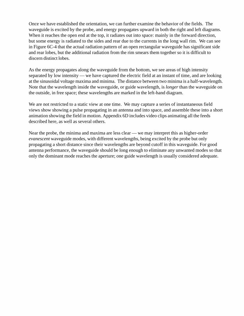
Once we have established the orientation, we can further examine the behavior of the fields. Thewaveguide is excited by the probe, and energy propagates upward in both the right and left diagrams.When it reaches the open end at the top, it radiates out into space: mainly in the forward direction,but some energy is radiated to the sides and rear due to the currents in the long wall rim. We can seein Figure 6C-4 that the actual radiation pattern of an open rectangular waveguide has significant sideand rear lobes, but the additional radiation from the rim smears them together so it is difficult todiscern distinct lobes.

As the energy propagates along the waveguide from the bottom, we see areas of high intensityseparated by low intensity — we have captured the electric field at an instant of time, and are lookingat the sinusoidal voltage maxima and minima. The distance between two minima is a half-wavelength.Note that the wavelength inside the waveguide, or guide wavelength, is longer than the waveguide onthe outside, in free space; these wavelengths are marked in the left-hand diagram.

We are not restricted to a static view at one time. We may capture a series of instantaneous fieldviews show showing a pulse propagating in an antenna and into space, and assemble these into a shortanimation showing the field in motion. Appendix 6D includes video clips animating all the feedsdescribed here, as well as several others.

Near the probe, the minima and maxima are less clear — we may interpret this as higher-orderevanescent waveguide modes, with different wavelengths, being excited by the probe but onlypropagating a short distance since their wavelengths are beyond cutoff in this waveguide. For goodantenna performance, the waveguide should be long enough to eliminate any unwanted modes so thatonly the dominant mode reaches the aperture; one guide wavelength is usually considered adequate.

WR-90 open waveguide at 10.368 GHz, by Zeland Fidelity

Figure 6C-4

Dish diameter = 10 λ Feed diameter = 1 λ

E-plane

H-plane

0 dB -10 -20 -30

Fee

d R

adia

tio

n P

atte

rn

W1GHZ 1998

0 10 20 30 40 50 60 70 80 90-90

-67.5

-45

-22.5

0

22.5

45

67.5

90

Rotation Angle aroundF

eed

Ph

ase

An

gle

E-plane

H-plane

specifiedPhase Center = 0 λ beyond aperture

0.3 0.4 0.5 0.6 0.7 0.8 0.90.25

10

20

30

40

50

60

70

80

90

1 dB

2 dB

3 dB

4 dB

5 dB

6 dB

7 dB8 dB

MAX Possible Efficiency with Phase error

REAL WORLD at least 15% lower

MAX Efficiency without phase error

Illumination Spillover

AFTER LOSSES:

Feed Blockage

Parabolic Dish f/D

Par

abo

lic D

ish

Eff

icie

ncy

%

The electric field of an open-ended circular waveguide, shown in Figure 6C-5, is very similar to theopen rectangular waveguide. However, the aperture field is more complex, requiring Besselfunctions for a mathematical description; Southworth2 skips ahead to diagrams like Figure 6C-1, andwe shall also resort to pictures. Like the rectangular guide, the aperture field intensity for thedominant mode is fairly uniform in the H-plane and has a maximum at the center in the E-plane, butthe maximum region has a constricted waist in the center, as seen in Figure 6C-5. Compare thiswith Figure 6C-1, which depicts the electric field as a series of lines, with closer spacing indicatinghigher field intensity. Also like the rectangular guide, there is high field intensity at the guide walls atthe top and bottom of the aperture; the one at the top of the aperture field plot is quite evident. Theresultant far-field radiation pattern has the large side and rear lobes as we saw in Figure 6.3-1.

Magnetic fields

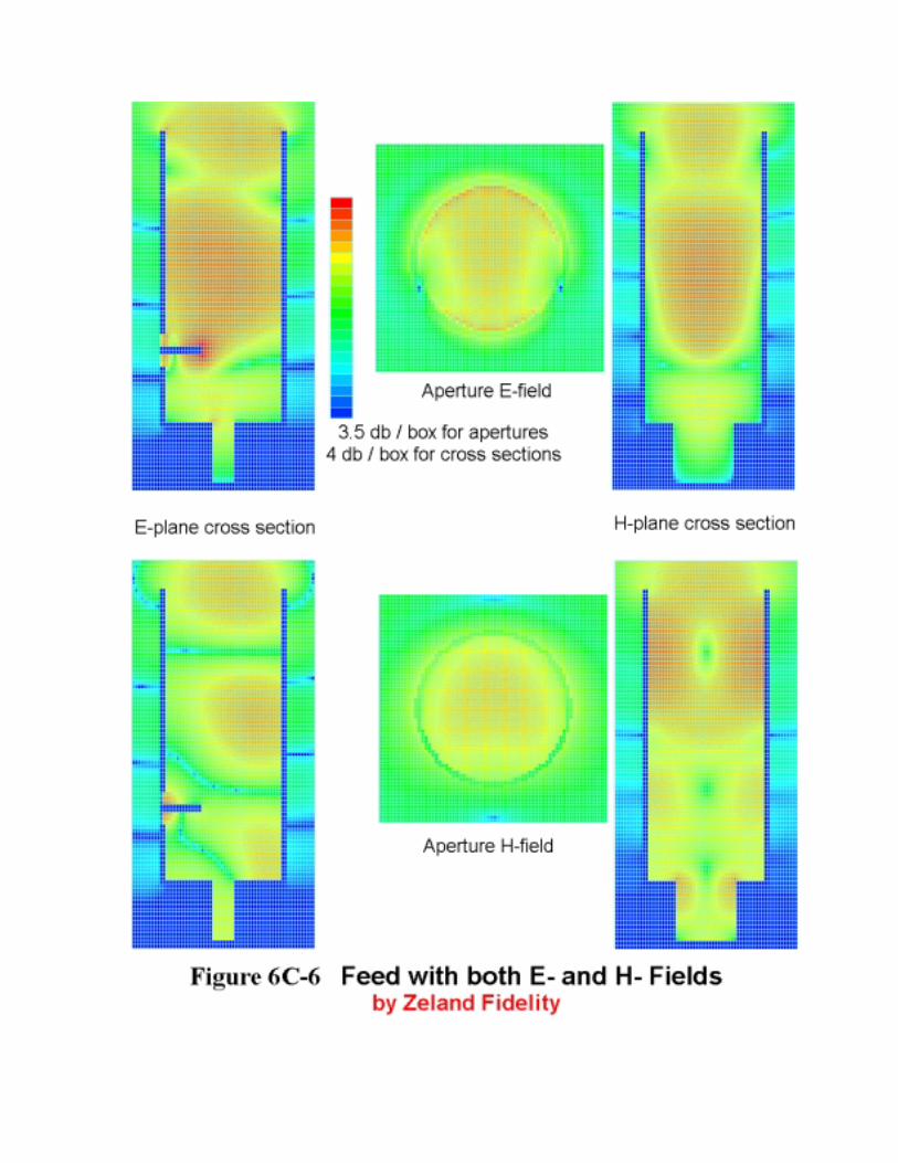
Any electromagnetic wave has both an electric field, or E-field, and an orthogonal magnetic field, orH-field. The electric field is more useful for our purpose: visualization and intuition. In many cases,the magnetic field might be more confusing than illuminating. In any case, I only saved the magneticfield for one example, a dual-band feed for 10 and 24 GHz by W5ZN6 described in Section 6.9. At10 GHz, this feed behaves just like an open-ended circular waveguide – the 24 GHz waveguidesection at the back is well beyond cutoff so it has essentially no effect at 10 GHz.

Figure 6C-6 shows both the electric fields and magnetic fields for this feed; the magnetic field plotsare below the electric. Decide for yourself whether the magnetic fields offer any additional insight.

Power flowing in a waveguide is the vector cross-product of the electric and magnetic fields, withboth magnitude and direction:

P = E x H

Since our color diagrams only show magnitude of the fields, they are of little use for the vectorcalculation. We can see that both electric and magnetic fields are strong in the aperture, so power isflowing, but we cannot discern the direction.

Sidelobe reduction in circular feeds

One of the primary objectives in feed antenna design is to maximize the radiation from the feed thatilluminates the reflector. Clearly, radiation to the sides and rear does not reach the reflector andshould be minimized. W2IMU7 stated that the goal of his dual-mode feed was to “cancel the electricfield at the aperture boundary,” — the high fields we see around the aperture in Figure 6C-5. Figure6C-7 shows the electric field in the W2IMU dual-mode feed. The second mode, excited by the flareto the larger diameter, is not clearly evident in the diagram, but the improvement in the aperture fieldis obvious. The field intensity is maximum in the center of the aperture and much less at the rim, orboundary, in all directions, with reduced field intensity along the outside of the guide walls. The endresult is the low sidelobe levels seen in Figure 6.5-1.

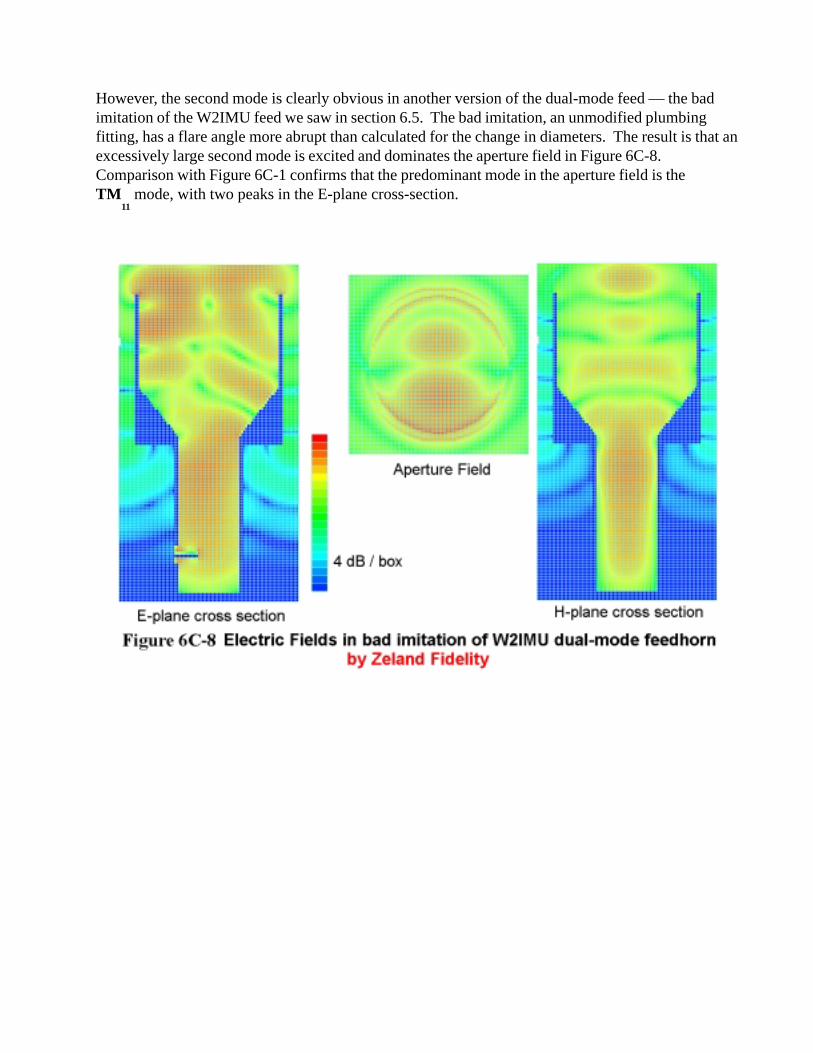
However, the second mode is clearly obvious in another version of the dual-mode feed — the badimitation of the W2IMU feed we saw in section 6.5. The bad imitation, an unmodified plumbingfitting, has a flare angle more abrupt than calculated for the change in diameters. The result is that anexcessively large second mode is excited and dominates the aperture field in Figure 6C-8.Comparison with Figure 6C-1 confirms that the predominant mode in the aperture field is theTM

11 mode, with two peaks in the E-plane cross-section.

Other feeds use choke rings to reduce unwanted lobes. The VE4MA feed, with fields shown inFigure 6C-9, and the Chaparral-type feeds, with fields shown in Figure 6C-10, both have fields in theaperture of the central circular waveguide similar to the plain open waveguide, with high fieldintensity on the rim at top and bottom. The choke rings reduce the field traveling back along theguide walls and so reduce radiation to the side and rear. The multiple choke rings of the Chaparral-type feed are effective over a wider bandwidth than the single-ring of the VE4MA feed, but widebandwidth is rarely important in amateur applications.

The left-hand diagram for the VE4MA feed shows an asymmetry in the field arriving at the aperture –an example of the effect of a short waveguide. One way to look at the problem, if the higher-ordermode explanation doesn’t help, is that the probe is closer to one wall than the other, so energy arrivesfirst at the rim wall nearer the probe. When the guide is longer, the difference in length becomes lesssignificant. Is this a real problem? Calculations on very short feeds often show a few degrees ofsquint in the radiation pattern, but since the illumination angle for these feeds is >100 degrees, theeffect is probably not significant.

Rectangular horns

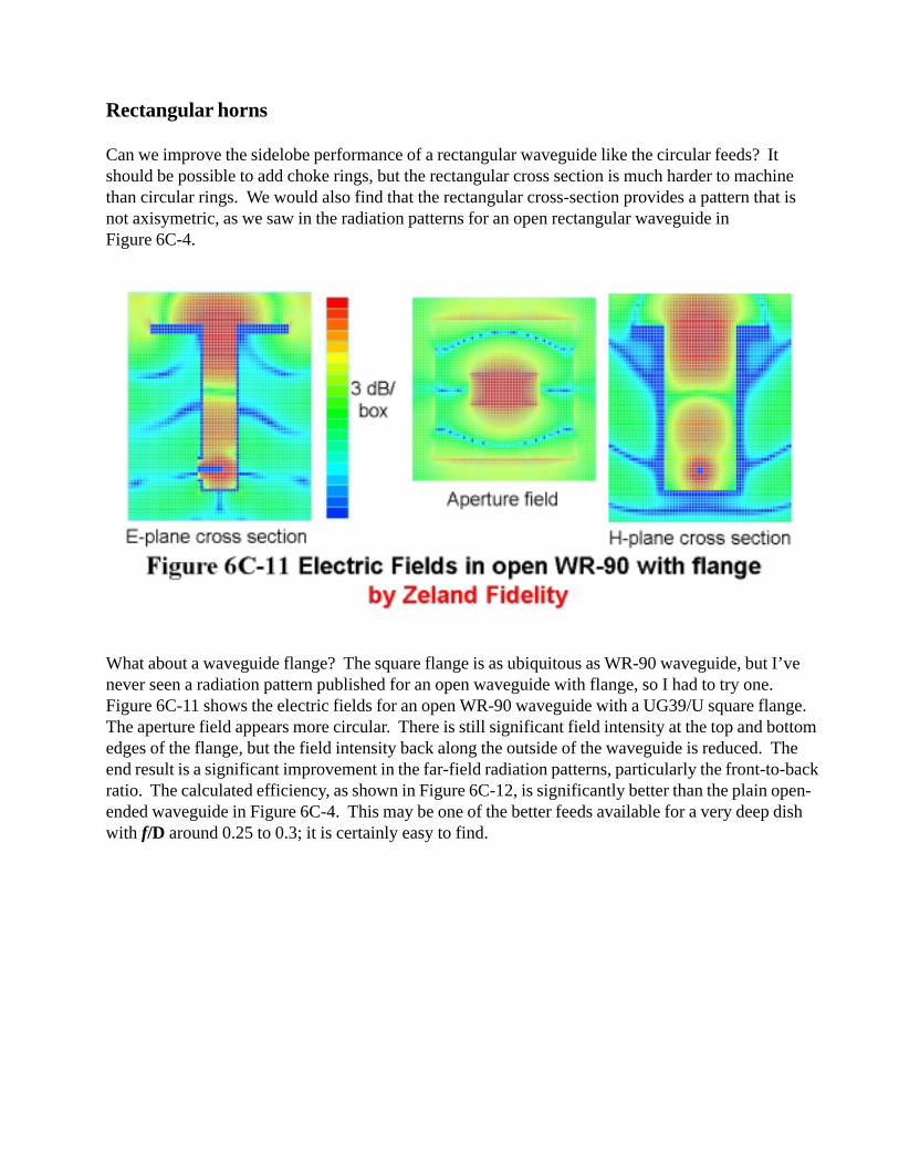
Can we improve the sidelobe performance of a rectangular waveguide like the circular feeds? Itshould be possible to add choke rings, but the rectangular cross section is much harder to machinethan circular rings. We would also find that the rectangular cross-section provides a pattern that isnot axisymetric, as we saw in the radiation patterns for an open rectangular waveguide inFigure 6C-4.

What about a waveguide flange? The square flange is as ubiquitous as WR-90 waveguide, but I’venever seen a radiation pattern published for an open waveguide with flange, so I had to try one.Figure 6C-11 shows the electric fields for an open WR-90 waveguide with a UG39/U square flange.The aperture field appears more circular. There is still significant field intensity at the top and bottomedges of the flange, but the field intensity back along the outside of the waveguide is reduced. Theend result is a significant improvement in the far-field radiation patterns, particularly the front-to-backratio. The calculated efficiency, as shown in Figure 6C-12, is significantly better than the plain open-ended waveguide in Figure 6C-4. This may be one of the better feeds available for a very deep dishwith f/D around 0.25 to 0.3; it is certainly easy to find.

WR90 open with square flange at 10.368 GHz

Figure 6C-12 by Zeland Fidelity

Dish diameter = 10 λ Feed diameter = 1 λ

E-plane

H-plane

0 dB -10 -20 -30

Fee

d R

adia

tio

n P

atte

rn

W1GHZ 1998

0 10 20 30 40 50 60 70 80 90-90

-67.5

-45

-22.5

0

22.5

45

67.5

90

Rotation Angle aroundF

eed

Ph

ase

An

gle

E-plane

H-plane

specifiedPhase Center = 0 λ beyond aperture

0.3 0.4 0.5 0.6 0.7 0.8 0.90.25

10

20

30

40

50

60

70

80

90

1 dB

2 dB

3 dB

4 dB

5 dB

6 dB

7 dB8 dB

MAX Possible Efficiency with Phase error

REAL WORLD at least 15% lower

MAX Efficiency without phase error

Illumination Spillover

AFTER LOSSES:

Feed Blockage

Parabolic Dish f/D

Par

abo

lic D

ish

Eff

icie

ncy

%

For a shallow dish with larger f/D, a rectangular horn can be a good feed. Figure 6C-13 shows theelectric field in the 10 GHz rectangular feedhorn for a DSS offset dish described in section 6.4. Thefield spreads out radially from the throat of the horn along the flare so that it is approaching aspherical wavefront as it reaches the aperture. Thus, the phase center, or apparent source of theradiation, is inside the aperture — for large horns, the phase center is close to the throat.

Like the open-ended waveguide, there is high field intensity at the top and bottom rim of the aperture,resulting in the E-plane sidelobes seen in section 6.4. Still, the horn concentrates the majority of theradiated power in the main lobe. By adjusting the flare angle in the two planes separately, we maymake the pattern more symmetric to provide an efficient feed.

Diagonal horns

A diagonal horn may be fed by a tapered transition from circular guide. We might expect the aperturefield to be somewhat similar to the field in the circular guide, as sketched in section 6.5. Thecalculated fields for a diagonal horn 0.73λ square with no flare, in Figure 6C-14, show no sign of theconstricted waist we saw in the circular guide; rather, the field has filled out toward all four corners,with higher field intensity at the top and bottom corners. The result is a radiation pattern with goodsymmetry in the E- and H-planes, shown in Figure 6C-15, and good calculated dish efficiency.Sidelobe level is somewhat higher in the E-plane due to the high field in the corners. The 45° planesdo not match the principal planes, since neither the aperture nor the fields are really axisymmetric, sothe pattern is not either. These results are comparable to the NEC2 calculations for a slightly smallerdiagonal horn, in section 6.5. The straight diagonal horn offers no real improvement on an opencircular waveguide, so the extra metalwork does not seem worthwhile.

Diagonal horn 0.73λ square, no flare, by Zeland Fidelity

Figure 6C-15

Dish diameter = 10 λ Feed diameter = 1 λ

E-plane

H-plane

45 degree planes0 dB -10 -20 -30

Fee

d R

adia

tio

n P

atte

rn

W1GHZ 1998

0 10 20 30 40 50 60 70 80 90-90

-67.5

-45

-22.5

0

22.5

45

67.5

90

Rotation Angle aroundF

eed

Ph

ase

An

gle

E-plane

H-plane

specifiedPhase Center = 0 λ beyond aperture

0.3 0.4 0.5 0.6 0.7 0.8 0.90.25

10

20

30

40

50

60

70

80

90

1 dB

2 dB

3 dB

4 dB

5 dB

6 dB

7 dB8 dB

MAX Possible Efficiency with Phase error

REAL WORLD at least 15% lower

MAX Efficiency without phase error

Illumination Spillover

AFTER LOSSES:

Feed Blockage

Parabolic Dish f/D

Par

abo

lic D

ish

Eff

icie

ncy

%

A diagonal horn with a gentle 14° flare to an aperture 1.4λ square, designed to feed an offset dish,has calculated fields shown in Figure 6C-16. The aperture field is slightly more uniform than theunflared horn, with a hint of a circular shape. The resulting far-field radiation patterns, shown inFigure 6C-17, have a good front-to-back ratio and low sidelobes in the E- and H-planes butsomewhat higher levels in the 45-degree planes. Calculated efficiency is very similar to thatcalculated using Physical Optics in section 6-5 for the same dimensions.

10 GHz diagonal feedhorn, 1.4λ square, 14° flare,

Figure 6C-14by Zeland Fidelity

Dish diameter = 14 λ Feed diameter = 1.4 λ

E-plane

H-plane

45 degree planes0 dB -10 -20 -30

Fee

d R

adia

tio

n P

atte

rn

W1GHZ 1998

0 10 20 30 40 50 60 70 80 90-90

-67.5

-45

-22.5

0

22.5

45

67.5

90

Rotation Angle aroundF

eed

Ph

ase

An

gle

E-plane

H-plane

specifiedPhase Center = 0.14 λ inside aperture

0.3 0.4 0.5 0.6 0.7 0.8 0.90.25

10

20

30

40

50

60

70

80

90

1 dB

2 dB

3 dB

4 dB

5 dB

6 dB

7 dB8 dB

MAX Possible Efficiency with Phase error

REAL WORLD at least 15% lower

MAX Efficiency without phase error

Illumination Spillover

AFTER LOSSES:

Feed Blockage

Parabolic Dish f/D

Par

abo

lic D

ish

Eff

icie

ncy

%

Penny feed

For a final example, we examine the electric field of a G4ALN “Penny” feed in Figure 6C-18. Thefield becomes bifurcated to radiate out the two slots on opposite sides of the waveguide, so thatradiation must emanate from two distinct sources, like Figure 1-2e; interference and sidelobes areinevitable. The result is that aperture field has poor axial symmetry, like the resultant radiationpatterns in section 6.7. The E-plane cross-section clearly shows diffraction of the field around theedges of the disk, resulting in the poor front-to-back ratio evident in section 6.7. The combination ofhigh sidelobes and poor front-to-back ratio reduces the useful radiation reaching the reflector, so thatdish efficiency with this feed is poor.

Summary

We have examined the calculated electric fields in and around some popular feed antennas to betterunderstand the operation of these antennas. These examples illustrate different features found in thenear field, so that we might better interpret near-field plots of other feeds. The goal is to help usdevelop a better intuition for antenna operation.

References

1. Zeland Software, Inc. http://www.zeland.com

2. Southworth, George C., Principles and Applications of Waveguide Transmission, van Nostrand,1950.

3. E.V. Jull, Aperture Antennas and Diffraction Theory, Peter Peregrinus Ltd., 1981.

4. R.W.P. King, H.R. Mimno, & A.H. Wing, Transmission Lines, Antennas, and Wave Guides,McGraw-Hill, 1945, pp. 254-263.

5. “Fourier Waveform Analysis,” Reverence Data for Radio Engineers, Sixth Edition, Howard W.Sams, 1975, Chapter 44.

6. J. Harrison, W5ZN, “W5ZN Dual Band 10 GHz / 24 GHz Feedhorn,” Proceedings of MicrowaveUpdate ’98, ARRL, 1998, pp. 189-190.

7. R.H. Turrin, (W2IMU), “Dual Mode Small-Aperture Antennas,” IEEE Transactions on Antennasand Propagation, AP-15, March 1967, pp. 307-308. (reprinted in A.W. Love, ElectromagneticHorn Antennas, IEEE, 1976, pp. 214-215.)