w2061

J. Webster (ed.), Wiley Encyclopedia of Electrical and Electronics EngineeringCopyright c© 1999 John Wiley & Sons, Inc.

CONTINUOUS-PHASE MODULATION

Continuous-Phase Modulation

Continuous-phase modulation (CPM) is a general form of digital phase modulation. The earliest digital phasemodulation is the phase-shift keying (PSK) and was established by the mid-1960s. The modulation method isboth linear and memoryless. A PSK signal is generated by shifting the phase of a carrier signal at signalinginterval boundaries between a predetermined set of phase values to represent the digital information that isbeing transmitted. The information-carrying phase is constant in each interval except for discontinuous jumpsat the beginning of each signaling interval. However, such abrupt switching from one phase to another resultsin relatively large spectral side lobes, and consequently, requires a large frequency band to transmit the signal.But, in many practical applications, the available radio spectrum is limited. This fact naturally imposes thedevelopment of spectrum efficient digital signaling techniques. Various methods were proposed in 1970s in theinterest of reducing the bandwidth, constituting a general class of digital phase-modulation techniques (1,2). Inthis class, the carrier phase is constrained to change in a variety of continuous fashion from symbol to symbolunlike that of PSK signals, hence the name continuous phase modulation. The continuous nature of their phaseprovides spectral efficiency compared to the PSK modulated signals, with a varying degree of spectral roll-offfactors. CPM signals are named with respect to the shape of their continuous phase transitions. Examplesinclude minimum-shift keying (MSK), tamed frequency modulation (TFM), and the well-known Gaussianminimum-shift keying (GMSK), which is adopted by global system for mobile communications (GSM).

The continuous-phase nature of CPM signals also introduces memory into the transmitted signal andoffers power gain over PSK signals. CPM achieves all these (spectral and power performance) yet with constantenvelope, which is suitable for nonlinear amplification and is an important attribute in satellite, terrestrialdigital radio, and mobile radio communications. This is another advantage of CPM that made it a populartransmission technique in the last two decades. Consequently, intrinsic to CPM is its continuous phase and theresulting memory, providing spectral efficiency and power gain over their PSK counterparts, respectively.

Signal and System Descriptions

It is essential for a proper understanding of CPM to resort to its mathematical description, and it is necessaryto introduce some terms to establish a systematic classification. To begin with, let us describe the transmittedconstant envelope CPM signal at the nth signaling interval after Aulin and Sundberg (3) as

1

2 CONTINUOUS-PHASE MODULATION

where φ(t, αn ) is the information carrying phase and given by

in which αn is the M-ary modulation symbol corresponding to the nth input xn, drawn from the set { ±1, ±3,. . ., ± (M − 1 )} with the relation αn = 2xn − M + 1 . For example, the modulation symbols for a binary ( M= 2 ) CPM are ±1 while taking values ±1, ±3 for a quarternary system (M = 4). That is, for a sequence ofquarternary input data x = {0, 1, 2, 3}, the modulation symbols are assigned as α = {−3, −1, 1, 3} . E denotesthe symbol energy, T the symbol interval, f 0 the carrier frequency, and π0 is an arbitrary constant phase shift,which without loss of generality can be set to zero in the case of coherent transmission. The vaable h is referredto as modulation index, which is related to the size of phase variation φ(t, αn ), and g(t) is the instantaneousfrequency pulse function. Defining the waveform q(t) as baseband phase pulse

the information-carrying phase of the CPM signal φ(t, αn) in Eq. (2) can be written as

where it is assumed that the pulse g(t) is of finite duration and has length L, hence occupying the interval(0, LT ). The first term on the right-hand side of Eq. (4) governs the change of the phase in response to themodulation symbol αn . The second term is the accumulated phase prior to the input αn, which is constant overthe symbol interval. As seen from Eq. (4), the information-carrying phase φ(t, αn ) at the nth symbol intervaldepends not only on the present modulation symbol αn but also all the transmitted symbols prior to αn . Moreprecisely, the initial value of the phase depends on all the previously transmitted symbols, while the shape ofits transition at the nth interval is influenced by αn as well as the L − 1 symbols prior to αn . It is clear fromEqs. (3) and (4) that the nature of the frequency or phase pulse defines a particular CPM scheme. It is thereforeapparent that an infinite variety of CPM signals can be generated by choosing different pulse shapes g(t) andmodulation index h and the alphabet size M . For example, continuous-phase frequency shift keying (CPFSK)is a special case of CPM, which uses the rectangular pulse g(t) . Another example is a special case of CPFSKwith modulation index h = 0.5, which is the scheme known as MSK. However, it is worth nothing here thatg(t) and q(t) are closely related as seen in Eq. (3), and can be used interchangeably to define a CPM scheme.In order for the modulation to be causal, the phase pulse is chosen such that q(t) = 0 for t ≤ 0 . The frequencypulse is also normalized so as to integrate to 1

2 , that is, q(t) = 12 for t ≥ LT . From Eq. (4), the maximum phase

change in a symbol interval would then be ( M − 1)hπ radians.CPM schemes are classified into two categories depending on the length of their frequency pulse g(t) .

If g(t) extends over only one symbol interval, that is, g(t) = 0, t > T, the CPM signal is called full-responseand corresponds to the case L = 1. It is called partial-response CPM when g(t) spills over more than oneinterval, which corresponds to the case L > 1 . To illustrate the structure of CPM and its performance, mainlythe rectangular (REC), the raised-cosine (RC), and the half-cycle sinusoid (HCS) frequency pulseunctions areused in the subsequent sections. These pulse names are commonly used as LREC, LRC, and LHCS, with

CONTINUOUS-PHASE MODULATION 3

Fig. 1. Various frequency and phase pulse functions. Phase pulse or its derivative frequency pulse characterize CPMschemes with their error and spectral performance.

Fig. 2. Frequency and the corresponding phase pulse shapes given in Fig. 1 with L = 1, corresponding to the full-responsecase.

L representing the length of the pulses in terms of symbol interval T. For instance, an RC pulse extendingover three symbol intervals is represented as 3RC. Figure 1 shows the equations for different frequency pulsefunctions g(t) with their corresponding phase functions q(t). To visualize these pulses, Fig. 2 shows theircorresponding shapes for the 43ull-response (L = 1) case.

Figure 3 illustrates both the full- and the partial-response RC frequency and phase pulse shapes forcomparison. Note that g(t) frequency pulses are normalized such that in both cases they integrate to 0.5. Thismeans that for a binary scheme (M = 2), the maximum phase change in a symbol interval will be only πhradians.

The Structure of CPM Signals

Thus far, we have given a general description of CPM. Now, let us gain better insight into the CPM signal and tothe spectral performance it offers over PSK modulation. For this purpose, we have chosen a binary PSK (BPSK)


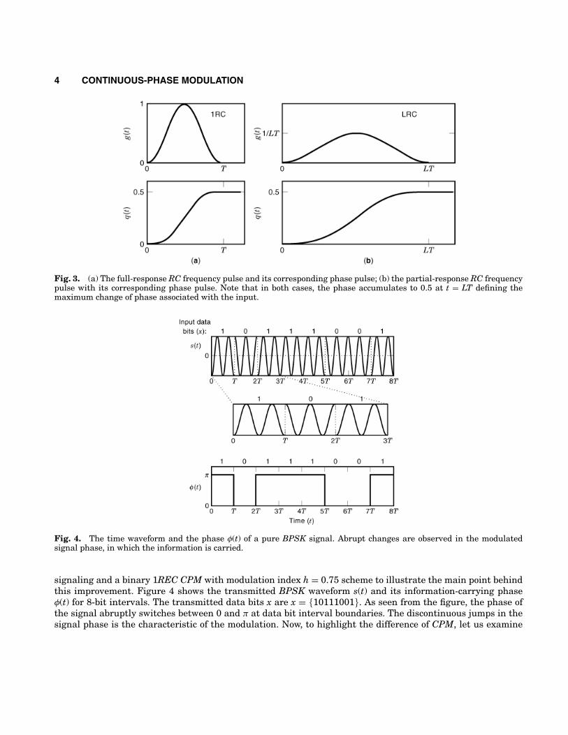
Fig. 3. (a) The full-response RC frequency pulse and its corresponding phase pulse; (b) the partial-response RC frequencypulse with its corresponding phase pulse. Note that in both cases, the phase accumulates to 0.5 at t = LT defining themaximum change of phase associated with the input.

Fig. 4. The time waveform and the phase φ(t) of a pure BPSK signal. Abrupt changes are observed in the modulatedsignal phase, in which the information is carried.

signaling and a binary 1REC CPM with modulation index h = 0.75 scheme to illustrate the main point behindthis improvement. Figure 4 shows the transmitted BPSK waveform s(t) and its information-carrying phaseφ(t) for 8-bit intervals. The transmitted data bits x are x = {10111001}. As seen from the figure, the phase ofthe signal abruptly switches between 0 and π at data bit interval boundaries. The discontinuous jumps in thesignal phase is the characteristic of the modulation. Now, to highlight the difference of CPM, let us examine


Fig. 5. The time waveform and the phase φ(t, α) of a CPM signal. The scheme is 1REC and the information bearing phasechanges in a continuous manner from interval to interval. This may result in a better error and spectral performancecompared to the PSK case.

the waveforms when the same data bits are transmitted by the chosen CPM scheme. Figure 5 illustrates thetime waveform of the transmitted binary CPM signal, and the information carrying phase φ(t, α) correspondingto the data bits x for 8-bit intvals. The transmitted modulation symbols α corresponding to the input data bitsx are α = {1 − 1111 − 1 − 11} as shown in the figure. The envelope of the transmitted signal is constantas in the BPSK case, but the transmitted signal phase no longer exhibits abrupt changes. As seen from thefigure, the signal phase associated with the input data changes continuously, and hence yields the underlyingspectral performance. We refer readers to have a close inspection of Fig. 5 to have a good understanding ofEqs. 1 2 3 4.

Let us give another example to illustrate why of the spectral performance offered by CPM, in which the2RC ( L = 2 ) frequency pulse is used to transmit the data. As is clear from the pulse shape, the CPM signalto transmit the data is of a partial-response type in this case. Figure 6 shows the individual smoothing phasepulses for the transmission of the same input data used in Fig. 5, and the resulting transmitted phase φ(t, α)in Eq. (4) for 2RC scheme with h = 0.75 in (a) and (b), respectively. In producing φ(t, α) in the figure, the inputbit prior to t = 0 is assumed to be 1. For the same data being transmitted, Fig. 6 also illustrates the 1RECscheme, with dotted lines for comparison. One can see that the phase transitions in 2RC case is much smoothercompared to that in 1REC case. Now, let us have a look at the power spectral density (PSD) of the illustratedBPSK, 1REC, and 2RC CPM schemes to see their individual spectral performance. Figure 7 shows the PSDfor the three schemes. It is clear from the figure that the 2RC scheme has better spectral side lobes. Abruptchanges observed in the phase of the BPSK signal imposed larger spectral occupancy. But the continuousnature of the CPM schemes improves the spectral side lobes, and the smoother the phase trajectory the betterthe spectral performance, as observed. It is therefore clear that as much as the continuity, also the smoothnessof the transmitted phase pulses plays an important role on the spectral performance, making their choice tobe of crucial importance. Comparing Figs. 4, 5, 6, 7 provides good insight and helps to better understand thenature of CPM and the spectral improvement it offers over PSK modulation.


Fig. 6. (a) Illustration of the individual partial-response (L = 2) phase pulses corresponding to each input bit, (b) thetransmitted resultant phase. Each input bit defines its own contribution to the total transmitted signal phase.

Fig. 7. Power spectral density of different schemes. Spectral improvement is clear with partial-response signaling. The2RC scheme is superior to both 1REC CPM and the BPSK.

Phase Tree. The information-carrying phase φ(t, α) illustrated before, such as in Fig. 5, corresponds to aunique data stream over 8T intervals. It is instructive to consider all possible values of the modulation symbolsα over an interval, and sketch the set of phase trajectories corresponding to these symbols commencing with acommon initial phase at time t = 0. This is a useful way of visualizing CPM, which results in a so-called phase


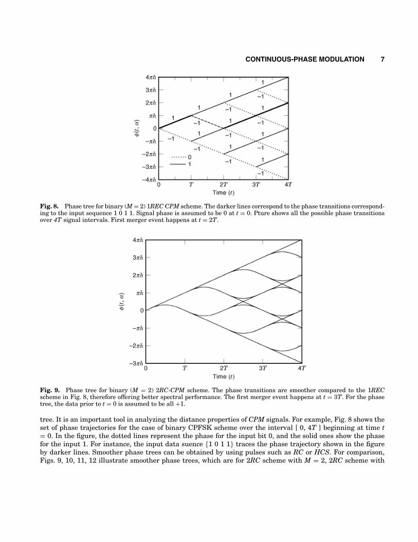
Fig. 8. Phase tree for binary (M = 2) 1REC CPM scheme. The darker lines correspond to the phase transitions correspond-ing to the input sequence 1 0 1 1. Signal phase is assumed to be 0 at t = 0. Pture shows all the possible phase transitionsover 4T signal intervals. First merger event happens at t = 2T.

Fig. 9. Phase tree for binary (M = 2) 2RC-CPM scheme. The phase transitions are smoother compared to the 1RECscheme in Fig. 8, therefore offering better spectral performance. The first merger event happens at t = 3T. For the phasetree, the data prior to t = 0 is assumed to be all +1.

tree. It is an important tool in analyzing the distance properties of CPM signals. For example, Fig. 8 shows theset of phase trajectories for the case of binary CPFSK scheme over the interval [ 0, 4T ] beginning at time t= 0. In the figure, the dotted lines represent the phase for the input bit 0, and the solid ones show the phasefor the input 1. For instance, the input data suence {1 0 1 1} traces the phase trajectory shown in the figureby darker lines. Smoother phase trees can be obtained by using pulses such as RC or HCS. For comparison,Figs. 9, 10, 11, 12 illustrate smoother phase trees, which are for 2RC scheme with M = 2, 2RC scheme with


Fig. 10. Phase tree for quarternary (M = 4) 2RC-CPM scheme. The phase transitions are smoother compared to the 1RECscheme. The maximum change of phase in an interval increased compared to the schemes with M = 2 in Figs. 8 and 9. Thefirst merger event happens at t = 3T as in the case of M = 2, L = 2 in Fig. 9. Note that the first merger depends on only theparameter L. For the phase tree, the data prior to t = 0 is assumed to be all +3.

Fig. 11. Phase tree for binary (M = 2) 3RC-CPM scheme. The phase transitions are smoother compared to the schemeswith L = 1 and L = 2 in Figs. 8 to 10, and the first merger is at t = 4T. For the phase tree,he data prior to t = 0 is assumedto be all +1.

M = 4, 3RC scheme with M = 2, and 3RC scheme with M = 4. Note that the phase axis is scaled in termsof 2πh by treating the modulation index h as a real number, so that the trees shown can be employed for anymodulation index.

Note from the figures that the phase tree exhibits M-ary branching from each phase trajectory every Tseconds, and therefore there are M N distinct phase paths at the end of N symbol intervals. It is clear that


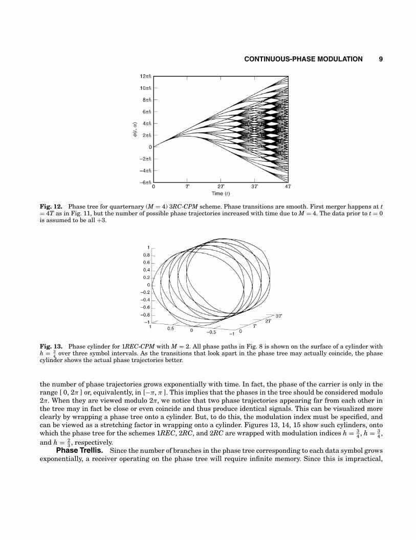
Fig. 12. Phase tree for quarternary (M = 4) 3RC-CPM scheme. Phase transitions are smooth. First merger happens at t= 4T as in Fig. 11, but the number of possible phase trajectories increased with time due to M = 4. The data prior to t = 0is assumed to be all +3.

Fig. 13. Phase cylinder for 1REC-CPM with M = 2. All phase paths in Fig. 8 is shown on the surface of a cylinder withh = 3

4 over three symbol intervals. As the transitions that look apart in the phase tree may actually coincide, the phasecylinder shows the actual phase trajectories better.

the number of phase trajectories grows exponentially with time. In fact, the phase of the carrier is only in therange [ 0, 2π ] or, equivalently, in [−π, π ]. This implies that the phases in the tree should be considered modulo2π. When they are viewed modulo 2π, we notice that two phase trajectories appearing far from each other inthe tree may in fact be close or even coincide and thus produce identical signals. This can be visualized moreclearly by wrapping a phase tree onto a cylinder. But, to do this, the modulation index must be specified, andcan be viewed as a stretching factor in wrapping onto a cylinder. Figures 13, 14, 15 show such cylinders, ontowhich the phase tree for the schemes 1REC, 2RC, and 2RC are wrapped with modulation indices h = 3

4 , h = 34 ,

and h = 23 , respectively.

Phase Trellis. Since the number of branches in the phase tree corresponding to each data symbol growsexponentially, a receiver operating on the phase tree will require infinite memory. Since this is impractical,


Fig. 14. Phase cylinder for 2RC-CPM scheme in Fig. 9 with h = 34 over three symbol intervals. Compare the phase cylinder

with that in Fig. 13 to see the effect of partial response on the shape of actual phase trajectories.

Fig. 15. Phase cylinder for 2RC-CPM with M = 2 and h = 23 . Compare the phase cylinder with that of Fig. 14 to see the

effect of modulation index h on actual phase trajectories.

the modulation index is restricted to be a rational number as h = p/q where p and q are integers that haveno common factors. This constraint ensures that phase trees collapse into a finite state phase trellis, whichcan then be explored by the Viterbi algorithm in the form of a trellis decoder Aulin (4). To explore the statedescription for CPM, let us rewrite Eq. (4) as


where

and

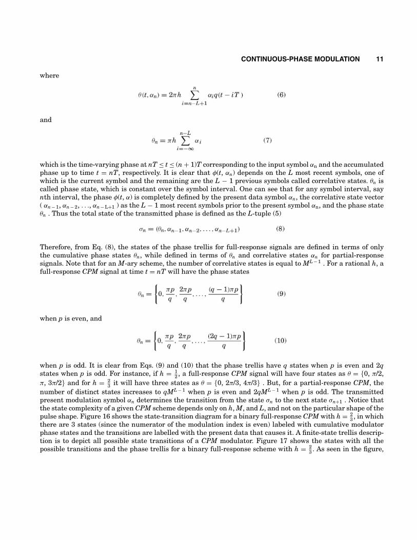
which is the time-varying phase at nT ≤ t ≤ (n + 1)T corresponding to the input symbol αn and the accumulatedphase up to time t = nT, respectively. It is clear that φ(t, αn) depends on the L most recent symbols, one ofwhich is the current symbol and the remaining are the L − 1 previous symbols called correlative states. θn iscalled phase state, which is constant over the symbol interval. One can see that for any symbol interval, saynth interval, the phase φ(t, α) is completely defined by the present data symbol αn, the correlative state vector( αn − 1, αn − 2, . . ., αn − L+1 ) as the L − 1 most recent symbols prior to the present symbol αn, and the phase stateθn . Thus the total state of the transmitted phase is defined as the L-tuple (5)

Therefore, from Eq. (8), the states of the phase trellis for full-response signals are defined in terms of onlythe cumulative phase states θn, while defined in terms of θn and correlative states αn for partial-responsesignals. Note that for an M-ary scheme, the number of correlative states is equal to ML − 1 . For a rational h, afull-response CPM signal at time t = nT will have the phase states

when p is even, and

when p is odd. It is clear from Eqs. (9) and (10) that the phase trellis have q states when p is even and 2qstates when p is odd. For instance, if h = 1

2 , a full-response CPM signal will have four states as θ = {0, π/2,π, 3π/2} and for h = 2

3 it will have three states as θ = {0, 2π/3, 4π/3} . But, for a partial-response CPM, thenumber of distinct states increases to qML − 1 when p is even and 2qML − 1 when p is odd. The transmittedpresent modulation symbol αn determines the transition from the state σn to the next state σn+1 . Notice thatthe state complexity of a given CPM scheme depends only on h, M, and L, and not on the particular shape of thepulse shape. Figure 16 shows the state-transition diagram for a binary full-response CPM with h = 2

3 , in whichthere are 3 states (since the numerator of the modulation index is even) labeled with cumulative modulatorphase states and the transitions are labelled with the present data that causes it. A finite-state trellis descrip-tion is to depict all possible state transitions of a CPM modulator. Figure 17 shows the states with all thepossible transitions and the phase trellis for a binary full-response scheme with h = 2

3 . As seen in the figure,


Fig. 16. State-transition diagram for a binary full-response CPM with h = 23 . There are only three phase states since the

numerator of the modulation index is even. When the signal phase at the beginning of an interval is 0, at the end of thesignal interval becomes 4π/3 if the input bit is 0 as illustrated. Recall that the modulation symbol α = −1 corresponds tothe data input 0.

Fig. 17. The state transitions and the phase trellis for binary 1REC scheme with h = 23 in Fig. 16. Phase trellis is shown

for the scheme, on which the influence of the input 1 0 1 1 1 on the change of phase state is traced.

Fig. 18. State-transition diagram for the binary scheme in Fig. 17 with a change of only L = 2, making the schemepartial-response. Note that the number of phase states are the same, but the total number of states due to the correlativestates are now 6. Transition from one state to another depends on the present phase state and the transmitted symbol inthe previous interval.


Fig. 19. The phase trellis for the binary partial-response CPM with L = 2 and h = 23 in Fig. 18. The phase trellis has

six states whereas there were only three states in the full-response case in Fig. 17. The trace shows the phase transitioncorresponding to the input 1 0 1 1 1.

Fig. 20. Phase tree for binary 2RC scheme with h = 23 . This is for the scheme in Fig. 18 with RC pulse shape. The phase

and the correlative states are marked on the tree. The traced trajectory corresponds to the input data 1 0 1 1.

a trellis structure called phase trellis is obtained by appending this state trellis side by side, each of whichrepresents a symbol interval. In the figure, a trellis path is also traced that represents the transition of thetransmitted phase corresponding to the input data (1 0 1 1 1). Let us consider another example for which theparameters are L = 2, M = 2, and h = 2

3 , and illustrate its state-transition diagram. Figure 18 shows thestate-transition diagram for the considered scheme, in which the number of states is qM L − 1 = 3 × 22 − 1 = 6.In this case, note that the states are labeled with a cumulative state and a data component (the data prior tothe present one). For instance, if the modulator state is σn = (2π / 3, − 1) and the current input is a symbol+1, then the next cumulative state becomes 0 radians, and the next data state (correlative state vector) is +1.Namely, the next state vector is σn = (0, 1). Figure 19 illustrates the phase trellis for a binary partial-responsescheme with L = 2 and h = 2

3 . The same input data example is emphasised also in this figure, assuming the


Fig. 21. Signal-space diagram for a full-response CPM signal with h = 14 and h = 2

3 . There are only eight phase states forh = 1

4 and three phase states for h = 23 . Since the scheme is of constant envelope, start and the end points of the possible

phases reside on a circle.

accumulated phase θn = 0 and αn − 1 = 1. Finally, to clarify the connection between phase tree, phase trellis,and the impact of modulo 2π and rational modulation index, let us redraw the phase tree for the binary 2RCexample with h = 2

3 . Figure 20 shows the tree labeled with the states assigned according to Eq. (8). Note that inthe figure, the phase trajectory corresponding to the input data in Fig. 19 is also traced. If the figure is closelyinspected, one can notice that there is repetition among the states, and there are only six of those that aredistinct. By writing down all the states that can be reached from each state, one ends up with the phase trellisshown in Fig. 19. In this way, the phase tree is converted into a phase trellis showing the phase transitionsfrom one state to another associated with the input data.

Geometric Representation of CPM. Unlike the PSK signals, CPM signals cannot be represented asdiscrete points in signal space, because of their continuous and time-varying phase. However, for constant-envelope CPM signals, only the possible starting and ending points of the phase trajectories can be marked ona circle. The number of marks will represent the number of cumulative phase states. Figure 21 shows a samplesignal-space diagram for a full-response CPM signal with h = 1

4 and h = 23 .

Basic CPM Transmitter

Considering Eqs. (2) and (3), it is seen that the transmitted waveform in Eq. (1) can be regarded as eithera frequency-modulated signal whose frequency is shaped by g(t) or a phase-modulated signal whose phase issmoothed by q(t) . Figure 22 illustrates this by a conceptual block diagram. For instance, this can be most easilyillustrated by using a CPM signal of a 1REC pulse with binary symbols by writing Eq. (1) as

with a constant carrier frequency f 0 and a time-varying phase, or as

with two different frequencies deviating from f 0 and a constant phase. However, in the sequel, we consider onlythe phase-modulation approach. It is of interest to translate this generic transmitter structure into a practical


Fig. 22. Schematic CPM transmitter. CPM signal can be generated by using either a phase- or a frequency-modulationapproach as illustrated.

solution. There are various methods to do this with their own limitations, one of which is the read-only memory(ROM) structure as the most straightforward form of implementation. The following introduces a generalimplementation of such a structure with some practical aspects. For this, the transmitted RF (radio-frequency)band-pass CPM signal in Eq. (1) can also be written by dividing it into its quadrature components as

where the quadrature components are

All the possible values of these quadrature I(t) and Q(t) pulse shapes for the scheme over one symbolinterval are then stored in I-channel and Q-channel ROMs, to be modulated by quadrature carriers of frequencyf 0 as in Eq. (13) after being converted to analog. Figure 23 illustrates this general way of implementing a CPMtransmitter. In the figure, the present data bit xn with the latest L − 1 bits and the phase state address theI-channel and the Q-channel ROMs to fetch the corresponding I(t) and Q(t) . A phase-state ROM provides theaddress for the phase state at the beginning of the signaling interval with a delay of one symbol interval (T),since the phase state at the beginning of the signaling interval is the phase state at the end of the previousinterval. One should note here that the I-channel and the Q-channel ROMs must be clocked with an m multipleof the symbol rate ( m/T ), where m is the number of samples per symbol interval. In general, each signal inthe ROM is identified by an address of M-ary data symbols of length L and a phase state number. For example,consider a CPM signal with parameters M = 4, L = 2, h = 3 using 8 samples/symbol representing each sampleby 8 bits. Since there are 2qML signal alternatives in each signal interval, for which h = p/q where p is odd asin the example, 6 × 42 signal alternatives exist. As 8 samples/symbol are used and each sample is representedby 8 bits, the total size of each of the I-channel ROM and the Q-channel ROM is then 6 × 42 × 8 × 8 = 6144bits. However, to reduce the size needed for the ROMs, by using Eqs. (6) and (7), I(t) and Q(t) in Eq. (14) can be


Fig. 23. Generic CPM ROM transmitter structure. Input bits and the phase state provided by the phase state ROM selectthe signal to be transmitted from the ROMs. I-channel and Q-channel signals are then swept out at a rate of m/T, wherem is the number of samples/symbol, converted to analog, and anti-aliasing filtered by a low-pass filter (LPF) to modulatethe quadrature carriers.

written as

This indicates that the phase transitions starting from only the zero phase state θn = 0 can be stored.Other pulse shapes starting from different phase states can be computed by a simple transformation as givenin Eq. (15). This would consequently reduce the size of each quadrature channel ROM by the number of phasestates. For the example above, a size of 1024 bits will be enough for each ROM in this case. Note that thisreduction in size may be quite significant depending on the value of h, especially for h values with largedenominators. But the penalty for this reduction is four multipliers and 2 small ROMs of 6 × 8 = 48 bits forcos(θn) and sin(θn) as in Eq. (15). From a practical point of view, such small ROMs are not available. But, as faras the very large scale integrated circuit (VLSI) implementation of the modulator is concerned, the requirednumber and size of ROMs can be implemented on-chip. However, Anderson et al. (5) give a variety of methodsfor implementing CPM transmitters.


Performance of CPM

The continuous trajectory of the phase of the transmitted CPM signal, shown in Fig. 5, builds memory intothe signal by introducing a certain dependency between transmitted phases, and thus improves the decodingperformance and side lobes. A power gain is obtained over pure PSK signals with a varying degree of spectralimprovement depending on the CPM signal parameters. The power gain is defined as 10 log10(d2

min/d2ref ) .

Here, d2min is the minimum Euclidean distance of the modulation scheme concerned and d2

ref is the minimumEuclidean distance for the reference pure (unfiltered) PSK modulation operating with the same energy per bit.For instance, the normalized d2

min for the pure BPSK is 2 and is 2.43 for the binary 1REC scheme with h =0.715 . Using this definition, the 1REC scheme obtains a 0.85 dB power gain over BPSK. This means that the1REC scheme needs 0.85 dB less energy per bit to obtain the same error performance compared to that for theBPSK modulation for the same noise power. In the following, we discuss the error and the spectral performanceof CPM signals.

Error Performance of CPM. For a digital communication system, the Euclidean distance (ED) isa useful parameter that gives a good measure of system performance (symbol or bit error probability). Acommonly used criterion for the system performance is the probability of symbol error, which is dominated bythe quantity corresponding to the minimum Euclidean distance. Assuming a Gaussian channel characteristicswith a large signal-to-noise ratio (SNR) Eb/N0, Anderson et al. (5) gives the error rate performance as

where

In Eq. (16), d2min is referred to as normalized squared minimum ED in the signal space, Eb denotes the bit

energy, and N0 represents the single-sided PSD of white Gaussian noise. To develop an ED expression for aCPM signal, let us suppose two signals s(t, α) and s(t, β) with their corresponding phase trajectories φ(t, α) andφ(t, β) of length N symbol intervals. The squared ED between these two signals, d2, is defined as


assuming 2πf 0 T � 1

It is seen from Eq. (19) that the ED is related to the difference between the phase trajectories and thesymbol energy E . However, it is convenient and desirable to express the distance in terms of the bit energy Eband to normalize the ED with respect to twice the bit energy as d2/2Eb, so that different schemes with differentalphabet size can be compared properly. So, we need to obtain the normalized squared ED, D2, from Eq. (19).Noting that E = Eb log2 (M) and writing the phase difference after Aulin and Sundberg (6) as φ(t, γ) = φ(t, α)− φ(t, β) in which γ = α − β and γi = αi − βi, D2 is obtained from Eq. (19) as

Since the minimum of the normalized squared Euclidean distances, d2min, is the dominant parameter on error

performance, one needs to find the minimum normalized squared Euclidean distance among all the possiblecombinations of symbol sequences α and β of length N (for N → ∞ ). Technically speaking,

in which α and β differs in the first symbol producing a nonzero difference symbol. It would be advantageous toknow the ultimately achievable d2

min for a CPM scheme before a system is actually designed, therefore savingcomputation power and time. In the following, for the error performance of CPM d2

min (h) and its upper boundsare considered for full-response and partial-response cases, respectively. We will plot the upper bounds on thedistances that each system can achieve, so that they can be compared to assess the error performance of bothschemes.

Full-Response Minimum Euclidean Distance Bounds. A helpful tool to compute d2min is the phase

tree. The phase tree for a binary 1REC scheme over the interval ( 0, 4T ) is shown in Fig. 24, where themodulation index is general. In the figure, the dotted lines corresponds to the phase trajectory correspondingto input symbol 0 with α = −1, and the solids to input symbol 1 with α = 1 . For the calculation of d2

min fora length of N symbol intervals by using Eqs. (20) and (21), all possible difference sequences corresponding tothe phase trajectory pairs must be considered, and the pairs of phase trajectories leaving the root node at t = 0must not coincide, namely γ0 �= 0 . The minimum of the all quantities obtained by using Eq. (21) is the desiredresult for an observation interval of N symbols.

Good candidates for a bound are infinitely long pairs of signals that merge as soon as possible. For thebinary 1REC scheme, a pair of a sequences are traced in Fig. 24 such that the two phase trajectories coincidefor all t ≥ 2T contributing zero quantity to the distance. This is called the first merger event, and determinesthe upper bound on d2

min for full-response schemes. Later mergers may also be considered in computing theupper bound, but they will all yield larger ED since the ED is a nondecreasing function of observation intervals.For a general M-level signals, Aulin and Sundberg (3) choose a difference symbol sequence as


Fig. 24. The phase tree for binary 1REC CPM with general h. The first inevitable merger is denoted by darker lines. Thismerger determines the ultimately achievable minimum Euclidean distance for the scheme.

and obtain the upper bound on the normalized squared ED, d2UB (h), for pulses having the symmetry property

g(t) = g(T − t), 0 ≤ t ≤ T (such as REC, RC, and HCS pulses), by using Eqs. (20) to (22) as

which for the REC pulse reduces to a simple analytic expression as

As seen also from Fig. 24, first mergers happen at t = 2T = (L + 1) T for all full-response schemes for anyvalue of modulation index. Occurring independent of h, such mergers are called inevitable mergers. However,there are also mergers prior to the first inevitable mergers, depending on the value of some specific modulationindices. Such mergers occur if there is a phase difference that equals to a nonzero integer multiple of 2π, andthe specific h value causing this merger is called weak modulation indices. Such modulation indices alwaysexist. For instance, h = 0.5 is a weak modulation index for the four-level 1REC scheme, producing a merger att = T prior to the first h-independent inevitable merger at t = 2T . At only such modulation indices, the d2

min(h) is always below d2

UB (h) (5). At a weak modulation index, if d2min (h) is particularly far below the upper

bound, the modulation index are called catastrophic.One can compute the upper bounds d2

UB (h) for different pulse shapes by using the Eq. (23) with numericalintegration. Figures 25, 26, 27 illustrate the d2

UB (h) for the three pulse shapes with M as parameter. As seenfrom the figures, no pulse shape always yields the better distance for all modulation indices. A scheme thatis good for small h values (h < 0.3 in the figures) yields poorer for large h values. The performance obviouslydepends on the frequency pulse shape g(t), the modulation index h, and the modulation level M. From thefigures, an important result is observed, which is that the distance increases with increasing M.


Fig. 25. Upper bounds on d2min (h) for binary 1REC, 1RC, and 1HCS systems with M = 2. The RC pulse performs better

for h < 0.5, but the REC pulse improves for h > 0.5. The 1REC with h = 0.5 is known as MSK, and the d2min for MSK is 2

as seen.

Fig. 26. Upper bounds on d2min (h) for binary 1REC, 1RC, and 1HCS systems with M = 4. With a slight difference,

distance for the REC pulse is inferior to the others. However, for the h values greater than approximately 0.3, the RECscheme performs better. Note that the distance bounds are greater for all h values compared to that for M = 2 case in Fig.25.

It is interesting to know the value of N for which the d2min (h) is reached, in other words, the smallest N

at which d2min,N (h) = d2

min(h). The growth of the d2min,N (h) with N is also an important parameter for system

design. A fast-growing d2min (h) with N is preferred since the receiver complexity and the time to demodulate

the signal increase with N. To assess the distance properties of a scheme, it would be interesting to visualize thebehavior of its d2

min,N(h). From Eq. (20), d2min (h) for a given observation interval length of N can be calculated


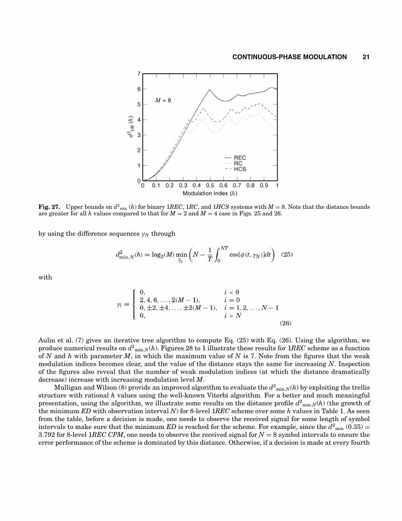
Fig. 27. Upper bounds on d2min (h) for binary 1REC, 1RC, and 1HCS systems with M = 8. Note that the distance bounds

are greater for all h values compared to that for M = 2 and M = 4 case in Figs. 25 and 26.

by using the difference sequences γN through

with

Aulin et al. (7) gives an iterative tree algorithm to compute Eq. (25) with Eq. (26). Using the algorithm, weproduce numerical results on d2

min,N(h). Figures 28 to 1 illustrate these results for 1REC scheme as a functionof N and h with parameter M, in which the maximum value of N is 7. Note from the figures that the weakmodulation indices becomes clear, and the value of the distance stays the same for increasing N. Inspectionof the figures also reveal that the number of weak modulation indices (at which the distance dramaticallydecrease) increase with increasing modulation level M.

Mulligan and Wilson (8) provide an improved algorithm to evaluate the d2min,N(h) by exploiting the trellis

structure with rational h values using the well-known Viterbi algorithm. For a better and much meaningfulpresentation, using the algorithm, we illustrate some results on the distance profile d2

min,N(h) (the growth ofthe minimum ED with observation interval N) for 8-level 1REC scheme over some h values in Table 1. As seenfrom the table, before a decision is made, one needs to observe the received signal for some length of symbolintervals to make sure that the minimum ED is reached for the scheme. For example, since the d2

min (0.35) =3.792 for 8-level 1REC CPM, one needs to observe the received signal for N = 8 symbol intervals to ensure theerror performance of the scheme is dominated by this distance. Otherwise, if a decision is made at every fourth


Fig. 28. Euclidean distance profile d2min,N (h) for CPFSK signal with M = 2. Minimum Euclidean diance increases with

the observation interval N. For N = 1, the distance is well below the upper bound. However, for N ≥ 2, the distance for thescheme mostly achieves the upper bound. h = 1 is a week modulation index for the scheme, as the distance suddenly dropsdown to 1. This is because an early merger happens at t = T. Note the steep decline on distance near the week modulationindex h = 1.

Fig. 29. Euclidean distance profile d2min,N (h) for CPFSK signal with M = 4. For the observation interval N ≥ 2, upper

bound is achieved for most values of h except for and near weak modulation indexes. Note that the number of weakmodulation index has increased compared to the scheme with the M = 2 case in Fig. 28.

symbol interval, the performance of the scheme will be determined by the distance 3.3. The length over whichthe signal must be observed to ensure the minimum ED for the system is called decision depth. As seen fromthe table that the decision depth for the signal depends on the modulation index.


Partial-Response Minimum Euclidean Distance Bounds. The procedure for constructing an upperbound on the minimum ED for partial-response schemes is similar to that of full-response schemes. The phasetree is again used to identify sequences that yield early mergers at a specific time and coinciding ever after.Since the two paths coincide after the merge event, note that the contribution of such paths to the ED afterthe merger will be zero. Recall from the full-response case that the time instant after which a phase differenceof two trajectories diverging at t = 0 can be made zero ever after is in general t = (L + 1)T. This time instantof first inevitable merger for the full-response case ( L = 1) is 2T, while it is T for a partial response schemewith L = 3. However, weak modulation exist as in the case of full-response schemes. One noticeable differenceof partial-response schemes in constructing the upper bounds on ED is that the upper bound is determined bythe first merger event in full-response case, while also later mergers contribute to the upper bound in partial-response case. The upper bound is found by taking the minimum of Euclidean distances associated with manymergers. Aulin and Sundberg (7) state that no mergers are needed to be considered later than the Lth.


Fig. 30. Euclidean distance profile d2min,N (h) for CPFSK signal with M = 8. For the h values greater than about 0.3,

upper bound is mostly not achieved as the number of weak modulation indexes has increased compared to that for the M= 2 and M = 4 cases in Figs. 28 to 29.

Aulin and Sundberg (7) gives the difference sequence for the mth merger as

satisfying �i = 0m γi = 0. To obtain the upper bound for a partial response, Eqs. (20) and (27) is used for m =

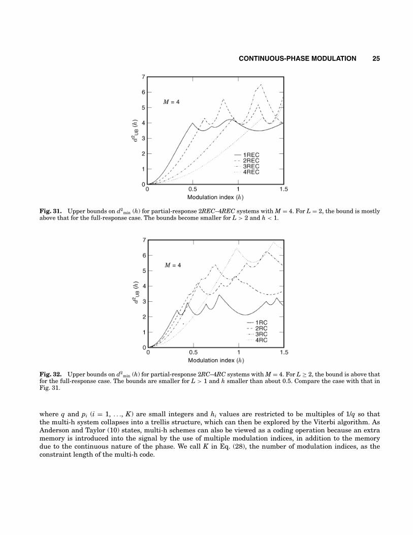
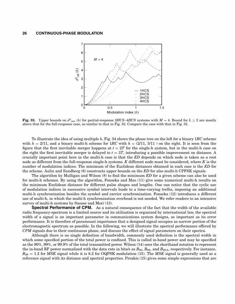
1, . . ., L with [ 0, (m+1)T ] integration intervals. Taking the minimum of all EDs yields the result. Figures 31,32, 33 illustrate the upper bounds for LREC, LRC, and LHCS partial-response schemes with M = 4 and L asparameters. One can notice from the figures that the upper bounds on the ED increase with increasing levelM as in the case of full-response systems. From the figures, another point to be made here is that the upperbounds becomes smaller for small h values with increasing L, but get larger for larger modulation indices.However, partial-response schemes achieves generally greater ED compared to the full-response schemes.

Multi-h CPM. To explain the use of multi-h CPM, let us confine our attention to the full-response caseonly. Remember that the upper bounds on the ED for full-response schemes is determined by the first inevitablemerger, which occurs at t = 2T except at weak modulation index values. Since the ED is a nondecreasingfunction of observation interval N, one way of increasing the ED is to delay the first merger. This generallyleads to an increased distance. This can be done by the use of properly chosen more than one modulationindex, by cyclically changing them in successive signaling intervals, hence the name multi-h. This idea wasfirst introduced by Miyakawa et al. (9) and generalized by Anderson and Taylor (10).

Modulation indices in multi-h schemes are chosen from a set of rational numbers with a common denom-inator q as


Fig. 31. Upper bounds on d2min (h) for partial-response 2REC–4REC systems with M = 4. For L = 2, the bound is mostly

above that for the full-response case. The bounds become smaller for L > 2 and h < 1.

Fig. 32. Upper bounds on d2min (h) for partial-response 2RC–4RC systems with M = 4. For L ≥ 2, the bound is above that

for the full-response case. The bounds are smaller for L > 1 and h smaller than about 0.5. Compare the case with that inFig. 31.

where q and pi (i = 1, . . ., K) are small integers and hi values are restricted to be multiples of 1/q so thatthe multi-h system collapses into a trellis structure, which can then be explored by the Viterbi algorithm. AsAnderson and Taylor (10) states, multi-h schemes can also be viewed as a coding operation because an extramemory is introduced into the signal by the use of multiple modulation indices, in addition to the memorydue to the continuous nature of the phase. We call K in Eq. (28), the number of modulation indices, as theconstraint length of the multi-h code.


Fig. 33. Upper bounds on d2min (h) for partial-response 2HCS–4HCS systems with M = 4. Bound for L ≥ 2 are mostly

above that for the full-response case, as similar to that in Fig. 32. Compare the case with that in Fig. 32.

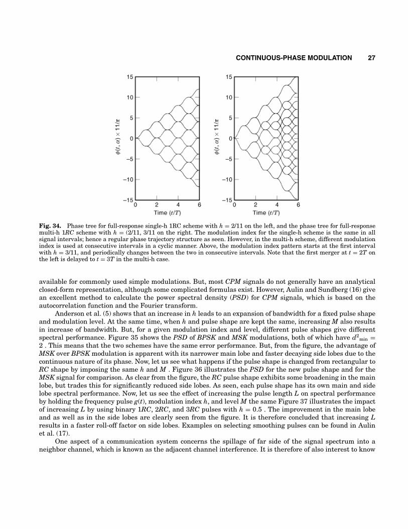
To illustrate the idea of using multiple h, Fig. 34 shows the phase tree on the left for a binary 1RC schemewith h = 2/11, and a binary multi-h scheme for 1RC with h = (2/11, 3/11 ) on the right. It is seen from thefigure that the first inevitable merger happens at t = 2T for the single-h system, but in the multi-h case onthe right the first inevitable merger is delayed to t = 3T, introducing a possible improvement on distance. Acrucially important point here in the multi-h case is that the ED depends on which node is taken as a rootnode as different from the full-response single-h systems. K different node must be considered, where K is thenumber of modulation indices. The minimum of the Euclidean distances obtained in each case is the ED forthe scheme. Aulin and Sundberg (6) constructs upper bounds on the ED for also multi-h CPFSK signals.

The algorithm by Mulligan and Wilson (8) to find the minimum ED for a given scheme can also be usedfor multi-h schemes. By using the algorithm, Fonseka and Mao (11) give some numerical multi-h results onthe minimum Euclidean distance for different pulse shapes and lengths. One can notice that the cyclic useof modulation indices in successive symbol intervals leads to a time-varying trellis, imposing an additionalmulti-h synchronization besides the symbol and carrier synchronization. Fonseka (12) introduces a differentuse of multi-h, in which the multi-h synchronization overhead is not needed. We refer readers to an intensivesurvey of multi-h systems by Sasase and Mori (13).

Spectral Performance of CPM. As a natural consequence of the fact that the width of the availableradio frequency-spectrum is a limited source and its utilization is organized by international law, the spectralwidth of a signal is an important parameter in communications system designs, as important as its errorperformance. It is therefore of paramount importance that a designed signal occupies as narrow portion of theelectromagnetic spectrum as possible. In the following, we will illustrate the spectral performance offered byCPM signals due to their continuous phase, and discuss the effect of signal parameters on their spectra.

Although there is no single definition of bandwidth, commonly used definition is the spectral width inwhich some specified portion of the total power is confined. This is called in-band power and may be specifiedas the 90%, 99%, or 99.9% of the total transmitted power. Wilson (14) uses the shorthand notation to representthe in-band RF power normalized with the data rate in bits/s as B90, B99, and B99.9, respectively. For instance,B99 = 1.2 for MSK signal while it is 8.2 for OQPSK modulation (15). The MSK signal is generally used as areference signal with its distance and spectral properties. Proakis (15) gives some simple expressions that are


Fig. 34. Phase tree for full-response single-h 1RC scheme with h = 2/11 on the left, and the phase tree for full-responsemulti-h 1RC scheme with h = (2/11, 3/11 on the right. The modulation index for the single-h scheme is the same in allsignal intervals; hence a regular phase trajectory structure as seen. However, in the multi-h scheme, different modulationindex is used at consecutive intervals in a cyclic manner. Above, the modulation index pattern starts at the first intervalwith h = 3/11, and periodically changes between the two in consecutive intervals. Note that the first merger at t = 2T onthe left is delayed to t = 3T in the multi-h case.

available for commonly used simple modulations. But, most CPM signals do not generally have an analyticalclosed-form representation, although some complicated formulas exist. However, Aulin and Sundberg (16) givean excellent method to calculate the power spectral density (PSD) for CPM signals, which is based on theautocorrelation function and the Fourier transform.

Anderson et al. (5) shows that an increase in h leads to an expansion of bandwidth for a fixed pulse shapeand modulation level. At the same time, when h and pulse shape are kept the same, increasing M also resultsin increase of bandwidth. But, for a given modulation index and level, different pulse shapes give differentspectral performance. Figure 35 shows the PSD of BPSK and MSK modulations, both of which have d2

min =2 . This means that the two schemes have the same error performance. But, from the figure, the advantage ofMSK over BPSK modulation is apparent with its narrower main lobe and faster decaying side lobes due to thecontinuous nature of its phase. Now, let us see what happens if the pulse shape is changed from rectangular toRC shape by imposing the same h and M . Figure 36 illustrates the PSD for the new pulse shape and for theMSK signal for comparison. As clear from the figure, the RC pulse shape exhibits some broadening in the mainlobe, but trades this for significantly reduced side lobes. As seen, each pulse shape has its own main and sidelobe spectral performance. Now, let us see the effect of increasing the pulse length L on spectral performanceby holding the frequency pulse g(t), modulation index h, and level M the same Figure 37 illustrates the impactof increasing L by using binary 1RC, 2RC, and 3RC pulses with h = 0.5 . The improvement in the main lobeand as well as in the side lobes are clearly seen from the figure. It is therefore concluded that increasing Lresults in a faster roll-off factor on side lobes. Examples on selecting smoothing pulses can be found in Aulinet al. (17).

One aspect of a communication system concerns the spillage of far side of the signal spectrum into aneighbor channel, which is known as the adjacent channel interference. It is therefore of also interest to know


Fig. 35. Power spectral density for MSK and BPSK systems. Due to the continuity of its phase, MSK has lower spectralsidelobes and it drops faster than that of BPSK.

Fig. 36. Power spectral density for MSK and 1RC scheme with h = 0.5. Both systems have the same modulation index.The only difference is the pulse shape. RC scheme has slightly larger first sidelobe, but exhibits a faster roll off in the latersidelobes.

the behavior of the spectrum in the side lobes for a complete description of the signal spectrum. Aulin et al. (3)define the fractional out of band power as a useful plot to show the behavior of the energy density outside theband concerned. The out of band power POB(B) is defined as


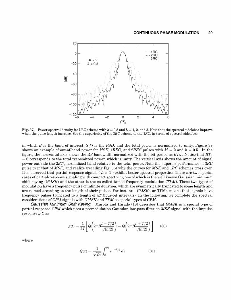
Fig. 37. Power spectral density for LRC scheme with h = 0.5 and L = 1, 2, and 3. Note that the spectral sidelobes improvewhen the pulse length increase. See the superiority of the 3RC scheme to the 1RC, in terms of spectral sidelobes.

in which B is the band of interest, S(f ) is the PSD, and the total power is normalized to unity. Figure 38shows an example of out-of-band power for MSK, 1REC, and 2REC pulses with M = 2 and h = 0.5 . In thefigure, the horizontal axis shows the RF bandwidth normalized with the bit period as BTb . Notice that BTb= 0 corresponds to the total transmitted power, which is unity. The vertical axis shows the amount of signalpower out side the 2BTb normalized band relative to the total power. Note the superior performance of 3RCpulse over that of MSK, and realize (recalling Fig. 36) why the curves for MSK and 1RC schemes cross over.It is observed that partial-response signals ( L > 1 ) exhibit better spectral properties. There are two specialcases of partial-response signaling with compact spectrum, one of which is the well known Gaussian minimumshift keying (GMSK) and the other is the so called tamed frequency modulation (TFM). These two types ofmodulation have a frequency pulse of infinite duration, which are symmetrically truncated to some length andare named according to the length of their pulses. For instance, GMSK4 or TFM4 means that signals havefrequency pulses truncated to a length of 4T (four-bit intervals). In the following, we complete the spectralconsiderations of CPM signals with GMSK and TFM as special types of CPM.

Gaussian Minimum Shift Keying. Murota and Hirade (18) describes that GMSK is a special type ofpartial-response CPM which uses a premodulation Gaussian low-pass filter on MSK signal with the impulseresponse g(t) as

where


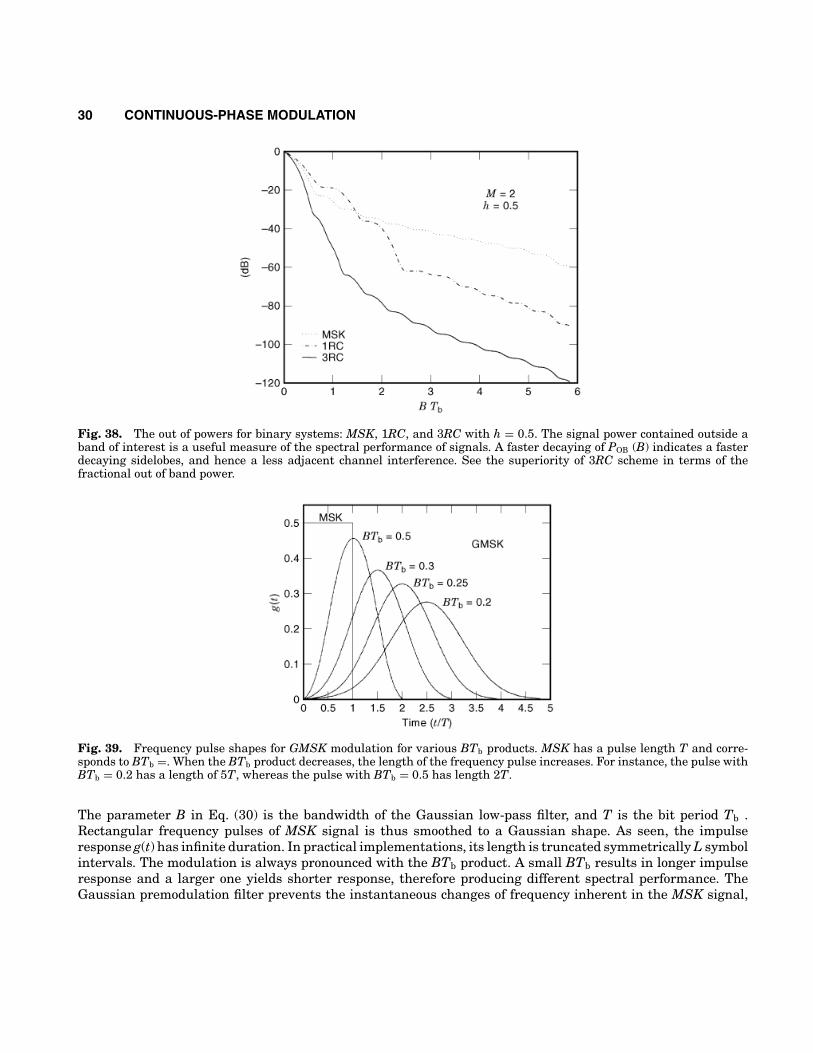
Fig. 38. The out of powers for binary systems: MSK, 1RC, and 3RC with h = 0.5. The signal power contained outside aband of interest is a useful measure of the spectral performance of signals. A faster decaying of POB (B) indicates a fasterdecaying sidelobes, and hence a less adjacent channel interference. See the superiority of 3RC scheme in terms of thefractional out of band power.

Fig. 39. Frequency pulse shapes for GMSK modulation for various BTb products. MSK has a pulse length T and corre-sponds to BTb =. When the BTb product decreases, the length of the frequency pulse increases. For instance, the pulse withBTb = 0.2 has a length of 5T, whereas the pulse with BTb = 0.5 has length 2T.

The parameter B in Eq. (30) is the bandwidth of the Gaussian low-pass filter, and T is the bit period Tb .Rectangular frequency pulses of MSK signal is thus smoothed to a Gaussian shape. As seen, the impulseresponse g(t) has infinite duration. In practical implementations, its length is truncated symmetrically L symbolintervals. The modulation is always pronounced with the BTb product. A small BTb results in longer impulseresponse and a larger one yields shorter response, therefore producing different spectral performance. TheGaussian premodulation filter prevents the instantaneous changes of frequency inherent in the MSK signal,


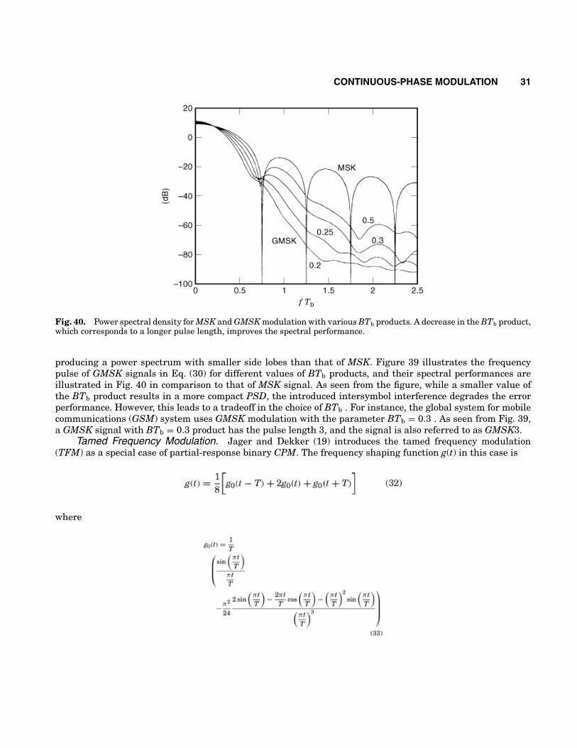
Fig. 40. Power spectral density for MSK and GMSK modulation with various BTb products. A decrease in the BTb product,which corresponds to a longer pulse length, improves the spectral performance.

producing a power spectrum with smaller side lobes than that of MSK. Figure 39 illustrates the frequencypulse of GMSK signals in Eq. (30) for different values of BTb products, and their spectral performances areillustrated in Fig. 40 in comparison to that of MSK signal. As seen from the figure, while a smaller value ofthe BTb product results in a more compact PSD, the introduced intersymbol interference degrades the errorperformance. However, this leads to a tradeoff in the choice of BTb . For instance, the global system for mobilecommunications (GSM) system uses GMSK modulation with the parameter BTb = 0.3 . As seen from Fig. 39,a GMSK signal with BTb = 0.3 product has the pulse length 3, and the signal is also referred to as GMSK3.

Tamed Frequency Modulation. Jager and Dekker (19) introduces the tamed frequency modulation(TFM) as a special case of partial-response binary CPM. The frequency shaping function g(t) in this case is

where


Fig. 41. Frequency pulse shape for TFM with length 4 and for GMSK with the same length.

Figure 41 shows the frequency pulse shape for TFM of length 4 (TFM4), with that of GMSK having the samepulse length 4 (GMSK4) or, equivalently, the parameter BTb = 0.25 for comparison. Figure 42 illustrates thePSD for TFM3 and GMSK3, in which the TFM signal has narrower main but a larger side lobes. However,Chung (20) gives an extension of TFM called generalized tamed frequency modulation (GTFM), which providesflexibility in selecting frequency pulse g(t).

General Remarks on CPM.

• d2min(h) increases with increasing M, and so does the signal bandwidth.

• d2min (h) generally increases with increasing h, and so does the signal bandwidth.

• Number of weak modulation indices increases with M, and most of them are catastrophic, and larger valuesof N are required to reach d2

UB (h) .• The first merger determines the upper bound on d2

min (h) for full-response systems with single-h except atweak modulation indices, but also later mergers must be taken into account for multi-h and partial-responsesystems.

• d2min (h) is a function of the pulse shape g(t), and the REC pulse generally gives greater distance results.

• No pulse shape performs better for the whole range of modulation indices.• CPM signals possess finite state with rational modulation indices, h = p/q .• K different case has to be considered to calculate the d2

min for multi-h schemes having K different modu-lation indices.

• Better d2min is generally obtained with close h values, which requires larger q values and therefore leads

to an increase in system complexity.• Larger values of N are required to reach d2

UB (h) for the modulation indices close to weak ones, which leadsto an increase in system complexity.

• Increasing L results in improved power spectrum for a given h, M, and g(t) .


Fig. 42. Power spectral density for TFM and GMSK modulation both with L = 3. With this parameter, TFM has a slightlynarrower main lobe whereas the GMSK has smaller sidelobes.

Topics in CPM

Rimoldi (21) introduced that any CPM system can be decomposed into a continuous-phase encoder as a lineartime-invariant sequential circuit and a memoryless time-invariant modulator. Campanella et al. (22) presentsan analytical procedure to minimize the effective bandwidth of a binary full-response CPM signal with respectto the shape of the frequency pulse for a given Euclidean distance. Campanella et al. (23) extends the work tothe partial-response case. Asano et al. (24) calculate the optimal signal shapes for full- and partial-responsesignals for various receiver observation intervals, using the performance measures of effective bandwidth andminimum distance. It has been also of interest to combine CPM signals with an external encoder to increasethe power–bandwidth performance of CPM schemes. In this way, extra memory has been introduced into CPMsignals in addition to their own memory due to the continuity of their phase, improving power as well as spectralperformance. Anderson and Sundberg (25) give an intensive survey of the advances in coded CPM modulation.Bhargava et al. (26) presents the calculation of orthogonal basis functions for a vector representation of CPMsignals in the signal space. Ertas and Poon (27) reports multi-h codes for rate 2

3 trellis codes combined withCPFSK signals for a better power–bandwidth performance. Ertas and Ali (28) construct upper bounds on thefree distance for Ungerboeck-type trellis codes combined with CPFSK signals.

The detection of CPM signals is a complex task, and received a great deal of attention in the literature.As the detection process is outside the scope of this article, we refer readers to Sasae and Mori (13) andthe references therein Anderson and Sundberg (25) and the references therein, and the Refs. 29 to 36 forthe synchronization, reduced complexity, coherent and noncoherent detection of multi-h, full-response andpartial-response CPM signals.


BIBLIOGRAPHY

1. F. Amoroso Pulse and spectrum manipulation in the minimum (frequency) shift keying (MSK) format, IEEE Trans.Commun., COM-24: 381–384, 1976.

2. M. Rabzel S. Pasupathy Spectral shaping in minimum shift keying (MSK) type signals, IEEE Trans. Commun., COM-26: 189–195, 1978.

3. T. Aulin C.-E. W. Sundberg Continuous phase modulation. Part I: Full response signaling, IEEE Trans. Commun.,COM-29: 196–209, 1981.

4. T. Aulin Viterbi detection of continuous phase modulated signals, Natl. Telecommun. Conf., Houston, TX, pp. 14.2.1–14.2.7, 1980.

5. J. B. Anderson T. Aulin C.-E. Sundberg Digital Phase Modulation, 1st ed., New York: Plenum, 1986.6. T. Aulin C.-E. Sundberg On the minimum Euclidean distance for a class of signal space codes, IEEE Trans. Inf. Theory,

IT-28: 43–55, 1982.7. T. Aulin N. Rydbeck C.-E. W. Sundberg Continuous phase modulation. Part II: Partial response signaling, IEEE Trans.

Commun., COM-29: 210–225, 1981.8. M. G. Mulligan S. G. Wilson An improved algorithm for evaluating trellis phase codes, IEEE Trans. Inf. Theory, IT-30:

846–851, 1984.9. H. Miyakawa H. Harashima Y. Tanaka A new digital modulation scheme: Multi-mode binary CPFSK, 3rd Int. Conf.

Digital Satellite Commun., Kyoto, pp. 105–112, 1975.10. J. B. Anderson D. P. Taylor A bandwidth-efficient class of signal-space codes, IEEE Trans. Inf. Theory, IT-24: 703–712,

1978.11. J. P. Fonseka R. Mao Multi-h phase codes for continuous phase modulation, Electron. Lett., 28: 1495–1497, 1992.12. J. P. Fonseka Nonlinear continuous phase frequency shift keying, IEEE Trans. Commun., COM-39: 1473–1481, 1991.13. I. Sasase S. Mori Multi-h phase-coded modulation, IEEE Commun. Mag., 29 (12): 46–56, 1991.14. S. G. Wilson R. C. Gaus Power spectra of multi-h phase codes, IEEE Trans. Commun., COM-29: 250–256, 1981.15. J. G. Proakis Digital Communications, 2nd ed., New York: McGraw-Hill, 1989.16. T. Aulin C.-E. Sundberg An easy way to calculate power spectra for digital FM, IEE Proc., Part F, 130: 519–526, 1983.17. T. Aulin G. Lindell C.-E. Sundberg Selecting smoothing pulses for partial-response digital FM, Proc. Inst. Electr. Eng.,

Part F, 128: 237–244, 1981.18. K. Murota K. Hirade GMSK modulation for digital mobile radio telephony, IEEE Trans. Commun., COM-29: 1044–

1050, 1981.19. F. Jager C. B. Dekker Tamed frequency modulation—A novel method to achieve spectrum economy in digital transmis-

sion, IEEE Trans. Commun., COM-26: 534–542, 1978.20. K.-S. Chung Generalized tamed frequency modulation and its application for mobile radio communications, IEEE J.

Select. Areas Commun., JSAC-2: 487–497, 1984.21. B. E. Rimoldi A decomposition approach to CPM, IEEE Trans. Inf. Theory, IT-34: 260–270, 1988.22. M. Campanella U. L. Faso G. Mamola Optimum bandwidth-distance performance in full response CPM systems, IEEE

Trans. Commun., COM-36: 1110–1118, 1988.23. M. Campanella, et al. Optimum bandwidth-distance performance in partial response CPM systems, IEEE Trans.

Commun., COM-44: 148–151, 1996.24. D. K. Asano H. Leib S. Pasupathy Phase smoothing functions for continuous phase modulation, IEEE Trans. Commun.,

COM-42: 1040–1049, 1994.25. J. B. Anderson C.-E. W. Sundberg Advances in constant envelope coded modulation, IEEE Commun. Mag., 29 (12):

36–45, 1991.26. V. K. Bhargava et al. Digital Communications by Satellite: Modulation, Multiple Access, and Coding, New York: Wiley,

1981.27. T. Ertas F. S. F. Poon Trellis coded multi-h CPM for power and bandwidth efficiency, Electron. Lett., 29: 229–230,

1993.28. T. Ertas F. H. Ali Upper bounds on the free distance for trellis coding combined with CPFSK signals, Electron. Lett.,

33: 1438–1440, 1997.29. W. P. Osborne M. B. Luntz Coherent and non-coherent detection of CPFSK, IEEE Trans. Commun., COM-22: 1023–

1036, 1974.


30. T. Aulin C. -E. Sundberg Partially coherent detection of digital full response continuous phase modulated signals, IEEETrans. Commun., COM-30: 1096–1117, 1982.

31. A. Stevenson T. Aulin C.-E. Sundberg A class of reduced complexity viterbi decoders for partial response continuousphase modulation, IEEE Trans. Commun., COM-32: 1079–1087, 1984.

32. J. Huber W. L. Liu An alternative approach to reduced complexity CPM receivers, IEEE J. Select. Areas Commun.,JSAC-7: 1437–1449, 1989.

33. A. Stevenson Reduced state sequence detection of partial response continuous phase modulation, Proc. Inst. Electr.Eng., Part-I, 138: 256–268, 1991.

34. S. Bellini G. Tartara Efficient discriminator detection of partial response continuous phase modulation, IEEE Trans.Commun., COM-33: 883–886, 1985.

35. M. K. Simon D. Divsalar Maximum likelihood block detection of noncoherent continuous phase modulation schemesusing decision feedback, IEEE Trans. Commun., COM-41: 90–98, 1993.

36. J. Huber W. L. Liu Data aided synchronization of coherent CPM receivers, IEEE Trans. Commun., COM-40: 178–189,1992.

TUNCAY ERTASUludag University

w2061

Documents