4 WAG-3 UPDATED AQUIFER MODEL CALIBRATION AND PREDICTIVE SIMULATIONS

The conceptual model of the HI interbed used to evaluate the RI/BRA model’s sensitivity to HI interbed parameterization is used as the basis for the updated aquifer model. The updated model was recalibrated to flow and transport with the goal of achieving or exceeding the same degree of model calibration as that of the RVBRA model. The updated model was then used as a predictive tool to reassess the betdgamma radiation emitting contaminants of potential concern (COPCs) identified in the RVBRA. The simulated contaminants included: iodine- 1 29, cobalt-60, cesium- 137, tritium, plutonium-24 1, strontium-90, and technetium-99.

4.1 Updated Model Calibration

The updated model used the same discretization as the rediscretized RI/BRA model used for the HI interbed parameter sensitivity analysis presented in Section 3.1. As with the RI/BRA model, the updated model incorporated a H basalt, HI interbed, upper I basalt, and lower I basalt structure. The upper I basalt was located north-west of the INTEC where the HI interbed is more steeply angled downward and is defined in approximately the top 25 m of the I basalt. Initial permeability values for the updated model’s H basalt were created from a spatial correlation analysis of pumping test hydraulic conductivity values in INEEL wells. Initial permeability values for the updated model’s HI interbed and I basalt were taken from the RVBRA model. Initial estimates of model transport parameters (porosity and dispersivity) were also taken from the RI/BRA model. Figure 4-1 illustrates the initial H basalt hydraulic conductivity field and includes the pumping test data.

The boundary conditions for the rediscretized model were specified flux at the surface from the Big Lost River and the RyBRA vadose zone model, zero flux at the model bottom, and specified pressure head on the model sides. Initial values for the specified head boundary conditions were created from performing a spatial correlation analysis on the 1999 head data set and interpolating these values onto the model perimeter. These initial model parameter estimates were then adjusted during model calibration.

C-5 1

~15000-

21 3000 ~

21 1000 -

209000 - - E - YI

f 207000 z r 4

205000 - a

203000.

2010001

199000 i 79900 E

L

Figure 4-1 Initial H basalt hydraulic conductivity estimate.

4.1.1 Aquifer Hydraullc Head Calibratlon

The best agreement with the spring 1999 hydraulic head data was obtained by slightly adjusting the model’s southeast specified head boundary condition and setting the H basalt minimum permeability to 1,000 mD (2.4 ft/day). A minimum H basalt permeability was needed to prevent extreme mounding from Big Lost River recharge. The updated model’s hydraulic bead RMS error over all wells within the simulation domain was 1.1 m. The updated model’s steady-state flow field with spring 1999 measured hydraulic bead is presented in Figures 4-2 and 4-3. It is interesting to note that recharge from the spreading areas located southwest of the Radioactive Waste Management Complex (southwest comer of the simulation domain) may be creating sufficient groundwater mounding to locally reverse the gradient. The average hydraulic head of four wells immediately east of the spreading area (RWMC-MA65, USGS-120, RWMC-MA66, and RWMC- MA13) is 1351.5 m and average hydraulic head of six wells immediately south of the RWMC (RWMC-MOlS, USGS-17, USGS-88, RWMC-MMD, USGS-119, and RWMC-MMS) is 1350.1 m suggesting water is flowing towards the SDA from the spreading area.

c-52

Figure 4-2 Rediscretized model hydraulic head (m) with spring 1999 observations.

c-53

21 3000.0

21 2600.0 \

21 2200.0

I 211800.0

E d

! v)

21 1400.0 7 5 !

z"

/." I

,/' o '359 63

t 21 1000.0

I 2 1 0600.0

21 0200.0

i / / 1- 1359.0 0 1359 25 o '359 86

0 1359 39 o 1359 36

o 135986 o 135982 135935

Figure 4-3 Rediscretized model hydraulic head (m) with spring1 999 observations near the INTEC.

4.1.2 CPP-3 Injection Weli Tritium Disposal Cafibration

decreasing basalt porosity to 3% and decreasing the initial basalt permeability estimates by a factor of two. Increasing the HI interbed permeability from 4 mD (0.01 Wday) to 70 mD (0.17 ft/day) and increasing the dispersivity to 20 m in the longitudinal direction 10 m in the transverse direction also improved the calibration. 70 mD (0.17 ftlday) was the average permeability obtained by pumping tests of the HI interbed (Frederick and Johnson, 1996).

The best agreement between simulated and observed tritium concentrations was obtained by

The rediscretized model's calibrated porosity was similar to the value needed to simulate the trichloroethene plume at the Test Area North (TAN) (Martian, 1997). Both the updated model and the TAN

c-54

model departed from previous groundwater modeling of the INEEL by using a variable thickness aquifer based on hydrogeologic data. The QR interbed provided the effective bottom of the contaminated aquifer at TAN and deep well temperature logs provided estimates the actively flowing aquifer below the INTEC. Inverse modeling of a large scale infiltratiodtracer test at the INEEL (Magnuson, 1995) also produced an approximately 3% large scale effective porosity for the fractured basalt.

Figure 4-4 illustrates the model predicted breakthrough and observed tritium concentrations for each calibration well. The updated model’s ModRMS error was 1.86 and the average correlation coefficient was 0.496 for all wells. The updated model’s hydraulic head calibration was significantly improved over the RVBRA calibration. The RMS error was decreased from 1.6 m to 1 . 1 m. However, the magnitude of the tritium calibration error was not significantly improved. The ModRMS error decreased from 1.98 to 1.86 m. The correlation coefficient was significantly improved over the R m R A model’s value. The correlation coefficient increased from 0.239 to 0.496. Both the R m R A and the updated model greatly overpredict tritium concentrations in wells USGS-39, USGS-35, and USGS-34 (upper crescent wells) and match concentrations in wells USGS-36, USGS-37, and USGS-38 (lower crescent wells). The order of magnitude decrease in observed tritium concentration between the upper and lower crescent wells suggests permeability may be lower near the upper crescent wells or local recharge from the Big Lost River may be changing the local gradient and diluting aquifer concentrations. In either case, hydrologic data is not available to explain the different tritium concentrations. Pumping tests of the crescent wells could assist in explaining the very different tritium concentrations seen between wells USGS-34 and USGS-36.

c-55

!

alotion=0.776 ModRMS-1.215

16m V I U

SirnhW Aqulfer Bottom - Flguw 4-4 Updated model tritium calibration wells breakthrough.

C-56

tion=0 959 ModRMS=0.947 orrelotion=0.960 ModRMS=l.415

9.0.10' 2.0.10. 1.0.w

0 1950 1wO is70 2Mo 1050 1wO

Y l W Y.U

=O 229 ModRMS-5 937 tion=-0 005 ModRMS=lO 920 1.0.10.

ma 1wO Y I Y

O ~ W + slmulsted at well screen - slrnuhed ~ u n w ~ o p - - - Slrmlsied N u b r Bnmm - Figure 4-4 contlnued Updated model tritium calibration wells breakthrough.

C-51

=0.896 ModRMS=0.483 -0.928 ModRMS=0.796

1963 iwo 1080 m Year

,132 ModRMS=2.155

ism 1080 ism iseo i9w m Y W

1963 ism 1970 IOM 1080 m 1963 two im Y I U Yaw

4.2 Updated Model Predictive Simulations

The betalgamma radiation emitting COPCs identified in the R m R A were simulated with the updated and recalibrated model. The simulated contaminants included: iodine- 129, cobalt-60, cesium- 137, tritium, plutonium-241, strontium-90, and technetium-99. Table 4- I lists each COPC, the half-life, the partition coefficients (Kd), the risk concentration, and the federal drinking water standard (MCL) concentration. The partition coefficient are those used in the RI/BRA analysis. The simulations used the water and COPC flux from the RI/BRA vadose zone simulations as the upper boundary condition. This upper boundary condition represents the soil contamination and backed up injection well sources. A complete description of contaminant sources can be found in the RUBRA (DOE-ID, 1997).

I Contaminant

The updated model simulation results are presented as peak contaminant concentration anywhere in the aquifer over the simulation period and as aquifer breakthrough concentrations at observation wells. Observed concentrations are graphically compared to simulated concentrations by overplotting the data on the breakthrough curves. Comparison of Pu-241 concentrations is not presented because the Pu-241 isotope has not been reported in the aquifer. Individual simulation results are presented in Sections 4.2.1 through 4.2.7 and the predictive simulations summary along with the cumulative risk of all simulated COPCs is presented in Section 4.2.8, Figures 4-5 and 4-6 illustrate well locations for comparison of simulated and measured contaminant concentrations.

I C4 Risk Federal Drinking Hd-life Sediment & Basalt K, Concentration Water Standard (wars) (mUd rocin, (Dcfi,

Table 4-1 Simulated betdgamma radiation emitting contaminants.

Iodine 129 (1-129) 1 1.57e+7 0. I 0. 1 0.261 1 .o

I Cesium 137 (Cs-137) 1 30.2 I 500. I 20. 1 1.52 I 200.

1 Tritium(H-3) \ 12.3 I 0. I 0. 1 671. I 20,000 I Plutonium 241 (PU-241) I 14.4 I 22. 1 0.88 I 0.145 1 63.**

I Strontium 90 (Sr-90) 1 29.1 1 12. I 0.48 1 0.859 I 8. I Technetium 99 (Tc-991 1 2.11e+5 I 0.2 I 0.008 I 34.3 I 900.

*Based on the 4mredyr critical organ dose as listed in the National Bureau of Standards Handbook 69 (HB69) and 2l/d 365d/yr consumption rate.

**Not listed in NBS 69. 1991 oroposed limits at 4mredyr effective dose eauivalent, which corresuonds to 4.66e-6 risk.

c-59

Figure 4-5 Well locations used for comparison of simulated and measured contaminant concentration.

C-60

2126001 I I

ousgs- 21 1' ocpp-4

/

21 1800

h

E

.- ? 21 1400

v

v)

L r

I 2

21 1000

2 1 0600

21 0200

o"sgs-12J

ousgs-057 ousgs-367 I o"Sgs-111 o u s g s - ' 1 6

209800 89500 89900 90300 90700 91100 91500

Eastings (m)

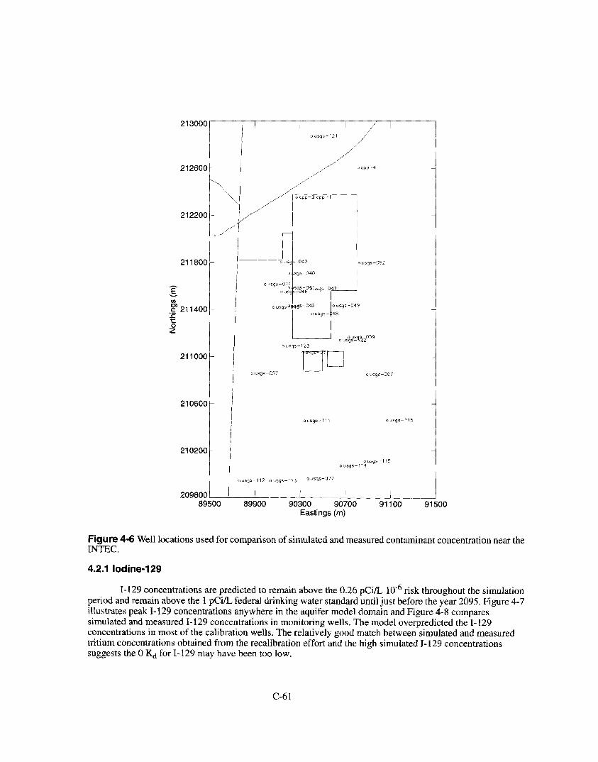
Figure 4-6 Well locations used for comparison of simulated and measured contaminant concentration near the INTEC .

4.2.1 lodine-129

1-129 concentrations are predicted to remain above the 0.26 pCiL risk throughout the simulation period and remain above the 1 pCiL federal drinking water standard until just before the year 2095. Figure 4-7 illustrates peak 1-1 29 concentrations anywhere in the aquifer model domain and Figure 4-8 compares simulated and measured I- 129 concentrations in monitoring wells. The model overpredicted the I- 129 concentrations in most of the calibration wells. The relatively good match between simulated and measured tritium concentrations obtained from the recalibration effort and the high simulated I- 129 concentrations suggests the 0 K d for 1-129 may have been too low.

C-6 1

Iodine-I29

0.0 ! -

35

Flgure 4-7 Peak aquifer concentration for 1-129 (red line is lo4 risk and blue line is MCL concentration).

C-62

axewed + simulated ai well Scnen - slmu!ated m u r r lop - - - Flgum 4-8 Comparison of simulated and measured 1-129 concentrations.

Slrrulated AquW sonom -

(2-63

0 b u ~ ~ ~ l - t s lmula tedatweu~nnn- S ~ U ~ W A ~ U H W T ~ ~ - - - Slmuhted Aquiler Botmm - Figure 4-8 continued Comparison of simulated and measured 1-129 concentrations.

C-64

0b.er.d + Slmu!aw at Well Scnan - Sirnuhid Aqutfer Top - - - Slmulaw Aquifer sOttOm - Flgum 4-8 contlnued Comparison of simulated and measured 1-129 concentrations.

C-65

4.2.2 Cobalt-60

The Co-60 concentrations exceeded the risk concentration during the period 1954 through 1980, but always remained below the MCL concentration. Figure 4-9 illustrates peak aquifer concentration anywhere in the aquifer and Figure 4-10 compares the simulated and measured Co-60 concentrations in monitoring wells. The model underpredicts concentrations in wells near the INTEC (USGS-40, USGS-43, USGS-44 and USGS-37). which indicates the fractured basalt &was too high. The simulated concentrations near the TRA are zero, which contradicts the observed concentrations. The updated and the RI/BRA models did not include Test Reactor Area (TRA) CO-60 sources and the simulated groundwater gradient does not allow a significant amount of the INTEC contamination to reach the TRA.

The WAG-7 preliminary R D R A model (Magnuson and Sondrup, 1998) calculated fractured basalt contaminant &s from fracture surface area rather than the mass of the rock matrix. The fracture surface area based &s basalt/sediment ratios were much less than the 1/25 ratio assumed in the INTEC RDRA analysis. For example, the WAG-7 Co-60 sediment & was 1,OOO mVg and the fractured basalt &was 6.5e-3 mVg.

Cobalt-60 100.0

75.0 - 2 8 s

8

-

'@ 50.0 - -

25.0- -

I -- I 0.01 rT

\I, \ 1

1950 1964 1979 lS94 2008 2022 2037 2052 2066 2080 2095 Year

Figure 4-9 Peak aquifer concentration for Co-60 (red line is risk and blue line is MCL concentration).

C-66

obwwd + srnulated a t w sueen - ~lmv~ated ~ q u ~ t r ~ o p - - - Figure 4-1 0 Comparison of simulated and measured Co-60 concentrations.

(2-67

4.2.3 Cesium-137

Cs-137 concentrations remained above the risk concentrations from 1954 through 2074, hut did not exceed the MCL concentration. Figure 4-1 1 illustrates peak aquifer concentrations anywhere in the aquifer during the simulation period and Figure 4-12 compares simulated and measured 0 - 1 3 7 concentrations in monitoring wells. As with the Co-60, the model under-predicts Cs-137 concentrations near the INTEC and concentrations are underpredicted by a greater extent than with Co-60. The large sediment & for Cs-137 (500 mVg) and corresponding large fracture basalt & (20 d g ) resulted in a more drastic overestimation of the fractured basalt &.

Cesium-137 200.01 I

2- 150.0- 8 '3 100.0- C 0 .-

1950 19& B4 2008 2022 2037 2052 2066 !080 2095 Year

FlgUm 4-1 1 Peak aquifer concentration for Cs-137 (red line is risk and blue line is MCL concentration).

C-68

~

iom

Simulated AquM Bonwn - Figure 4-12 Comparison of simulated and measured Cs-137 concentrations.

C-69

1980 1970 1980 -i WO ~

1980

+ ~ i m u i a t ~ at mi smwn - SirnuiatM ~ q o f f i r ~ o p - - - Simulated Aquw Bonwn - Figure 4-12 contlnued Comparison of simulated and measured Cs-137 concentrations.

C-70

Figure 4-12 continued Comparison of simulated and measured Cs-137 concentrations.

(2-71