Wage Divergence and Asymmetries in Unemploymentin a Model with Biased Technical Change

J. Muysken, M. Sanders* and A. Van ZonDepartment of Economics and MERIT

University of Maastricht

Abstract

In this article we assume two levels of skills and two classes of goods, one produced with atechnology requiring high skills, the other produced with a technology that can be operated byboth low and high skilled workers. Our model generates two distinct labour market regimes.In one regime we show technical change can be the cause of wage divergence between skilledand unskilled workers. This result is consistent with recent evidence on wage differentials.Adding the Phillips-effect shows this wage divergence can be “traded off” againstunemployment of low skilled workers, and hence explains evidence on skill asymmetries inunemployment. Under the alternative regime these effects do not exist but high skilledworkers may replace low skilled workers driving them out of their jobs.

Keywords

Skill biased technological change, job competition, wage divergence, low skilledunemployment.

* Corresponding author

P.O. Box 6166200 MD Maastricht, The Netherlandse-mail: m.sanders@algec.unimaas.nlphone number: +31 43 388 36 91

1

1. Introduction

Over the past decade or so, the labour market perspectives for low skilled workers haveworsened dramatically throughout the OECD. This problem has been widely recognised andmost authors agree that the causes for this deterioration of labour market perspectives are tobe found in the changing composition of labour demand. The OECD formulated the problemas: .... one of the most serious current challenges in the OECD area is the trend

shift in the composition of the demand for labour away from unskilled andtowards skilled labour. (OECD (1994))

Throughout the OECD, however, it is interesting to note the different manifestations of thisseemingly common shift in demand.

Unemployment is high and rising relatively for low-skilled workers in Europe (OECD(1994), Draper and Manders (1997)) as is the duration of their average unemployment spell(Muysken en Ter Weel (1998)). At the same time we find skilled workers in jobs that do notrequire their level of skill, the so called trickling down effect (CBS (1996)).

In the US and other Anglo-Saxon countries, on the contrary, overall unemployment is at anall time low. Low skilled workers still suffer a much higher unemployment rate relative totheir high skilled competitors (OECD (1994)). The most dramatic manifestation of the shiftingdemand, however, is through relative wages. In these countries they show a very strongtendency to diverge. A result that is almost absent in mainland Europe (OECD (1994)).

For understanding these developments two questions have to be addressed. First of all onehas to explain what may have caused the demand for low skilled labour to drop so sharplyover the eighties throughout the developed world. Then one can address the issue of thewidely different responses to this seemingly common cause.

In this paper we will address these issues by presenting a model that shows how biasedtechnical change might cause the relative demand for low skilled workers to drop, but alsoallows for two distinct labour market outcomes in response to this drop in relative demand.We show that the drop in demand can cause either strong wage divergence that can partiallybe traded off against asymmetric unemployment. Or it causes a trickling down effect of highskilled workers pushing low skilled workers out of their jobs, but relative wages remainstable.

Theoretical Background

Two possible reasons for the drop in the demand for low skilled workers have beendistinguished in the literature. On the one hand there are those that link the shift in demand tothe process of globalization and increasing trade with low wage/low skilled countries. Keyreferences are Leamer (1994,1995), Burtless (1994) and Lawrence and Slaughter (1993). Onthe other hand there are those that link this demand shift to pervasive changes in productiontechnology often linked to the IT-revolution. Some notable references are Krugman (1995),Jackman (1995), Howell (1995) and Agenor and Aizenman (1996). The issue remains to beresolved both in theoretical and empirical work on either approach.

Both approaches, however, can be traced back in the classical economic literature. Thetrade hypothesis follows from extensions and elaborations on the standard factor priceequalization theorem formulated by Stolper-Samuelson. The idea of job destruction by

Back in those days the distinction between skilled and unskilled labour was not made of course, but1

the idea of biases against one of the production factors remain valid even today.

2

technical change can be traced back all the way to Ricardo’s Principles and Marx’ Capitaland the ideas of technical bias have been formalised in Hicks’ Theory of Wages. The debate1

on the issue has never really conquered the lime light in economics but notable authors suchas Binswanger (1974a, 1974b), Kennedy (1964), Phelps (1966) and Salter (1960) havecontributed to a sizeable literature on the issue.

From the research available so far we cannot safely disregard either hypothesis and bothwill probably explain current events in the OECD partially. However in this paper weconcentrate on linking technological change to labour demand in a way that allows us to showa possible source of bias in technical change that may cause the shift in demand. The reasonfor our choice of focus is twofold.

First we simply find the idea of biases in technical change intuitively appealing. It seemsevident from casual observation that different forms of technical change involve a particularchange in the organisation of the productive process. Introducing a new product usuallyrequires the set up of a whole new production line, which requires a skilled labour force that iscapable of dealing with the unforseen problems that occur during this phase of introductionand commercialisation of the new product. As the product matures, the firm can develop andintroduce an interface that allows less skilled persons to perform the routine elements in theproduction process and makes the skilled workers more productive.

Secondly the OECD (1994) presents evidence that the importance of trade in explaining thechanges in employment are but a fraction of the impact of productivity changes throughout theOECD, which could be interpreted as evidence that technical change has a more profoundimpact on labour demand in general. Furthermore the relative size of intra OECD trade totrade with non-OECD countries seems to rule out a severe impact of wage competition fromlow wage countries at the aggregate level.

A final indication for the relative importance of the technical bias hypothesis comes fromFeenstra and Hanson (1997) who show there is also evidence of wage divergence indeveloping countries. Although circumstantial this evidence supports our intuition andjustifies our choice of focus.

On the issue of different responses, notably between mainland Europe and the US, abooming literature has developed over the last few years. Many authors have, and justly so,looked at the differences in wage formation and labour market institutions for an explanation(Teulings and Hartog (1998)) and indeed found that many of the differences in labour marketperformance can be explained.

Krugman (1994) was the first to address the issue and in his paper he argues Europe’slabour market rigidities imply an adjustment to the shifting demand in unemployment,whereas the flexible labour markets in the US translate this drop in demand into a decline inrelative (and even absolute) wages: “Moneyless America, Jobless Europe”. Appealing as thisstory seems, however, it does not explain the facts.

Nickell and Bell (1995) have shown European high unemployment is not explained by adrop in low skilled labour demand. Furthermore data from the OECD (1994) show highabsolute unemployment rates but these are not as skill biased as those in the United States asKrugman’s analysis would predict. In this paper we therefore set out to develop a model thatprovides an alternative and perhaps complementary explanation for the observed differencesin labour market responses.

In a later stage we hope to refine the model to deal with more skill levels or a continuum of skills. This2

will hopefully increase the plausibility and intuitive appeal of our model.

This setup is reminiscent of Krugman’s (1979) model of North-South Trade. 3

3

Outline

The challenge is now to build a model in such a way that technical change can cause bothwage divergence and low skilled unemployment or wage stability and the trickling down ofskills. In this article we assume two levels of skill and two classes of goods, one produced2

with a highly sophisticated technology requiring high skills, the other produced with arelatively simple technology that can be operated by both low and high skilled workers. Thusan asymmetry in employment opportunities is assumed.

Technical change can be introduced in the model by allowing the number of either class ofgoods to increase over time. The development of new products, labelled product innovation,causes the number of goods produced on high sophisticated technologies to increase. Theassumption is that producing a new good requires higher flexibility, higher problem solvingcapabilities and more creativity: in short, higher skills on behalf of the worker.

An expansion of the range of goods that can be produced with low skilled labour is labelledprocess innovation. One could think of technical change as an improvement in the interfacebetween production technology and the worker, thus allowing a low skilled worker to performcomplicated tasks, previously only manageable by high skilled workers. Not only does theinterface allow low skilled workers to become productive, it also allows the high skilledworkers to be more productive than before. New goods thus mature as their interface developsover time.3

Using this framework we show that technical change can be the prime cause of wagesdiverging between skilled and unskilled workers under a particular labour market regime. Aresult consistent with the empirical evidence on wage differentials in the Anglo-Saxon world.Adding Phillips-effects to the model shows wage divergence can be “traded off” againstincreasing relative unemployment of low skilled workers under this regime. This result couldexplain the empirical evidence on skill asymmetries in unemployment. The model , however,also yields a second regime in which wages do not diverge but high skilled people occupy jobsin the low skilled sector, consistent with the evidence on employment and wage patterns onmainland Europe. We show that under this regime a chimney effect will occur as long as skillmismatch exists. That is, as long as high skilled workers are employed on low skilled jobs,increasing high skilled jobs may alleviate low skilled unemployment.

The basic model with a competitive labour market is presented in section 2. The model isextended to include unemployment in section 3, whereas in section 4 technological change isintroduced and a comparative statics analysis is presented. Finally, some concluding remarksare made in section 5.

UMn

i1c�

i

1/�

0<�<1

UnHc�H�nLc

�L

1/�

Here we deviate from Krugman (1979) who assumes a one-on-one technology.4

4

(1)

(2)

2. The Basic Model

General Settings

Our simple economy consists of two types of households. We have consumers that consume arange of goods and derive utility thereof. The utility function was taken from Krugman (1979)and has the well known “love of variety” characteristics. All consumers are assumed identicaland are represented by an individual that maximises his and therefore total utility by choosingthe appropriate levels of consumption for each good, subject to his budget constraint.

The variety of goods is produced by a range of production units that can only bedistinguished on the basis of their technology determined input requirements. Some varietiescan only be produced by high skilled labour due to the sophistication of the productionprocess. Others are manufactured in a routine like manner and can thus be produced byemploying either high or low skilled workers. There are no other inputs in our model. Bothconsumers and producers can only distinguish between high- and low-tech goods. Within aclass of goods, however, the goods are perfectly symmetric both in terms of utility andproduction technology.

By assuming price taking behaviour on behalf of the consumer and monopolistic pricesetting by producers we find all high-tech goods command the same price, as do all low-techgoods, within their class.

The producers set prices given demand, wages and their production technology. By thesymmetry and diminishing returns assumed within classes their decision is reduced tochoosing an average output level for high and low-tech goods, where output per variety withina class is the same. In the following subsections we first analyse the consumer decision and4

the producers’ decisions in isolation. Then the goods market equilibrium can be derived. Byconfronting the labour demand that is derived from profit maximization with exogenous andendogenous labour supply respectively we can close the model and analyse the impact oftechnical change in comparative statics.

The Consumer Decision

Consumers maximize their utility. Assume a representative consumer whose utility is givenby:

where c is the consumption of good i and n is the number of varieties of goods produced and i

1/1+� the elasticity of substitution between two varieties. When we distinguish between aclass of goods that can be produced using high skilled labour and one in which both types oflabour can be used, we may write this utility function also as:

cH

cL

PH

PL

1�1

xL[l eL]� 0<�<1

xH[lHH]� 0<�<1

In a symmetric utility function consumers optimize by spreading consumption equally across all5

varieties that command the same price. Hence consumers consume the average amount of all varietieswithin each class and c =(c +c +...+c )/n .H h1 h2 hnH H

�>1. Some tentative evidence in Van Zon, Muysken and Meijers (1998) has shown this value is6

approximately 1.25 in the Netherlands between high and medium and medium and low level skills.

5

(3)

(4)

(5)

where subscripts H(igh) and L(ow) indicate the level of sophistication of the technology usedto produce those goods and c and c are the average amounts of consumption of high andH L

low sophisticated goods, respectively. Finally n and n indicate the number of varieties of5H L

both goods. We maximise the utility function subject to the simple (Walrasian) budgetconstraint, Y= P n c + P n c, where Y is income and P and P are the price levels forH H H L L L H L

both classes of goods. Then relative average consumption of high and low-tech goods is afunction of the relative price:

The Producers and Goods Market Equilibrium

Each variety is produced in a situation of profit maximisation under imperfect competition onthe product markets (varieties are heterogenous by assumption) and perfect competition on thelabour market. Labour (measured in efficiency units) is the only factor of productiondistinguished in the model.

We identify two groups of producers. As was mentioned above, the output of a variety ofhigh sophisticated goods can only be produced by employing high skilled labour. High skilledlabour not employed by the high tech producers is available for the production of lowsophisticated goods as is the entire supply of low skilled labour. The output of any varietyexhibits diminishing returns in the relevant input. Due to the symmetry in production within aclass of products and the diminishing returns, the average output per variety is equal to theoutput of any variety within that class. It can be written as a function of the labour input pervariety. Average output of a low sophisticated variety is given by:

Where l = ( L +� L )/n , is the labour input on all n low sophisticated varieties measured ineL L HL L L

efficiency units. L is the number of low skilled workers employed and L is the number ofL HL

high skilled workers on low sophisticated jobs. The latter workers are assumed to be � timesas efficient as low skilled workers. Equivalently for all n high sophisticated varieties output6

H

is equal to average output:

Where l = L /n is the amount of high skilled labour employed in the production of eachHH HH H

%HPHxHwHlHH

%LPLxLwLle

L

xH

xL

wH/PH

wL/PL

�

�1

PH

PL

wH

wL

���

1��

GME

w

P

6

(6)

(7)

(8)

(9)

Figure 1: Goods Market Equilibrium

high tech variety. Profits for both types of producers are given by:

Where w and w are the wages paid to one efficiency unit of high and low skilled labourH L

respectively. Producers now set prices to maximise profits given the relative demand for theirproduct (3), the production function (4) and (5) and wages. Standard optimization yields theprofit maximizing relative average supply as a function of relative prices and wages:

Equating relative average supply (8) and demand (3) yields the relative prices as a function ofrelative wages for which the goods markets clear:

Equation (9) describes the relative wage-price frontier for which the goods market is inequilibrium. Figure 1 shows this frontier, labeled GME, is a concave line through the origin inP,w-space, where P and w are the relative price and wage ratio respectively.

The Demand for Labour

A similar approach can be followed to derive the relativewage-price frontier for the labour market. Since labour isthe only factor of production in the model, it follows thatthe supply of a certain type of good directly generates acorresponding demand for the appropriate type of labour.

l DH

l DL e

wH/PH

wL/PL

11�

l SHH

l SL e

(L �

HLHL)/nH

(L �

L��LHL)/nL

PH

PL

wH

wL

(L �

HLHL)/nH

(L �

L��LHL)/nL

1�

w

P

LHL/L* H �

LMELHL=0

1

7

(10)

(11)

(12)

Figure 2: Equilibrium in the Labour Market

By substituting for output in (8) by (4) and (5), we can solve for the relative implied demandfor labour (in appropriately skilled efficiency units) as a function of the relative productwages:

Inelastic Labour Supply and Equilibrium in the Labour Market

We now first introduce exogenous labour supply to provide a benchmark case. When labour issupplied inelastic, relative supply in efficiency units can be written as:

Equating (10) and (11) yields the relative wage-price frontier for which the labour market is inequilibrium:

It can be verified in equation (12) that producers will set relative prices proportional torelative wages with a factor of proportion that depends on the relative availability of highskilled workers and the relative size of the high skilled sector. Equation (12) can berepresented in w,P-space as well. It traces out a linear upward sloping line on which the labourmarket is in equilibrium. The slope of the curve is, however, conditional upon the value forL and decreases as L increases. Figure 2 shows the Labour Market Equilibrium, LME,HL HL

conditional on L =0.HL

As we have mentioned above, L refers to the demand for high-skilled workers on low skilledHL

jobs. It can be shown from the first order conditions for low skilled producers that theseworkers will only be employed on these jobs when relative wages match relative efficiency,

LHL

L �

H

L �

H/nH

L �

L/nL

PH

PL

11��

1�1

�

�

�1 PH

PL

11�

�

L �

H/nH

L �

L/nL

w

P

LHL/L* H �

LMELHL=0

A

B

1

GME

8

(13)

Figure 3: The Complete Specialisation Equilibrium

that is L >0 can only occur when w /w ��. It is profitable to replace low skilled workers withHL H L

high skilled workers on low skilled jobs as long as the latter condition is a strict inequality. Onthe other hand, high skilled wages should always exceed those for low skilled jobs, that isw ��.w . Otherwise all high-skilled workers will seek employment on low skilled jobs.H L

Therefore an equilibrium with 0<L <L* is only possible for w /w =�. HL H H L

For the relative wage equal to �, equation (12) can be solved to yield skill mismatch,L /L* , as a function of relative prices only:HL H

The left quadrant in Figure 2 shows this relationship as a downward sloping curve with apositive intercept at the relative price level where the LME -curve intersects w /w =�. HL=0 H L

The reasoning above implies that for higher relative wages, i.e. w>�, no high skilled labourwill be employed on low-skilled jobs. Therefore the LME line with L =0 will be onlyHL

relevant for w>�, as is indicated by the thick line in Figure 2, from point A upwards.

The Equilibrium with Inelastic Labour Supply

In order to determine the simultaneous equilibrium of our model Figure 3 combines the goodsand labour market equilibrium wage-price frontiers. As the GME is a concave line in w,P-space and the LME is upward sloping and linear, we know there is a unique point ofLHL=0

intersection. From (11) we know this point of intersection moves to the right as the number ofhigh skilled workers in the low skilled sector increases, since this would rotate the LME curveclockwise. This implies there are two possible equilibria in the model. Figure 3 shows the straightforward case where the GME-curve intersects the LME-curve

above point A, the point of intersection of the GME-curve and the line w=�. In such anequilibrium the wages paid in the high skilled sector are too high for low tech producers tobenefit from their employment. This implies they will set L = 0 and relative wages nowHL

adjust to bring about equilibrium. The economy would remain in a point such as B and the leftquadrant shows the employment rate of high skilled workers in the low tech sector is 0. Hence

w

P

LHL/L* H �

LMELHL=0

A

C

1

LMELHL=LHL*

GME

LHL*/L* H

9

Figure 4: The Incomplete Specialisation Equilibrium

we label this equilibrium complete specialisation.Another possible equilibrium is illustrated in Figure 4 and prevails when the GME-curve

intersects with the LME -curve below point A. In such an equilibrium low tech producersLHL=0

find it attractive to employ high skilled workers. In the process of competing for high skilledworkers they will drive up the relative wages until w=�. This will rotate the LME-curve to

LME . The economy reaches an equilibrium at point C, where the GME-curve intersectsLHL=LHL*

with w=�. In such an equilibrium L /L* >0 (left panel) and there is positive skill mismatchHL H

L . We label this equilibrium incomplete specialisation. HL*

As can be seen from equations (9) and (12), the GME-curve does not change when laboursupply or the number of varieties change, whereas the LME-curve does. That is, the LME-curve moves clockwise both when L */L * and n /n increase. This implies that when lowH L L H

skilled labour is abundant, the ratio of high wages relative to low wages will be high and nohigh skilled labour will be employed on low skilled jobs. As one might expect, this tendencywill be reinforced by product innovations that increase n . For such innovations increase theH

relative scarcity of high skilled labour. We will discuss the impact of technical change more indetail in section 4.

3. Wage Formation and Unemployment

So far we have not allowed labour supply to respond to these wage adjustments and haveassumed zero unemployment, so unemployment rates can obviously not be compared. Thisissue will be addressed in the next sections by assuming endogenous labour supply andrepeating the analysis outlined above.

Wage Formation and Labour Market Equilibrium with Elastic Labour Supply

When we endogenise labour supply and allow for unemployment the results will obviouslychange, although not qualitatively. We will, for the purpose of this paper, abstract frommicroeconomic foundations underlying our labour supply conditions. For now we refer to f.e.Layard, Nickell and Jackman (1994) and put the exact derivation of our assumptions on theagenda for further research. Moreover, in the Annex to this paper we present an alternativeprocess of wage formation which leads to results similar to the present analysis.

Here we assume a process of wage bargaining, both by high-skilled workers and by low-skilled workers, taking each other’s wage as a reference, in the context of a right-to-manage

wH�wHL

1uHH

1u�

5

0<5<1 �>1

wL1�

wH

�

1uL

1u�

5

For simplicity we assume that unemployment benefits are equal to the wage that would have been7

earned when working, minus benefits from leisure. Therefore being unemployed is not a threat in thebargaining process.

Since we assume that in this wage bargaining process unemployment benefits do not pose any threat,8

high-skilled workers are indifferent between working on low skilled jobs or being unemployed.

Taking the parameters u*, � and 5 for both bargaining processes is just for convenience and does not9

alter the qualitative results.

10

(14)

(15)

model. High skilled workers will negotiate a wage, w , for the high skilled sector taking7H

demand for high skilled employment in that sector, L , into account and using as an outsideHH

option, the wage a high skilled worker can earn in the low skilled sector, �w = w .TheL HL

excess high skilled labour supply, which we assume to be the difference between exogenoustotal high skilled labour supply, L *, and the level of employment in the high skilled sector,H

will turn to the low skilled sector, where the low skilled wage is determined in a bargainingprocess by low-skilled workers.

The high skilled wages bargained in the high skilled sector are given by:

where u =(L *-L )/L * is the mismatch and unemployment rate of high skilled workers andHH H HH H

u* is the exogenous rate that high-skilled workers accept when their demands are met. The8

wage claim is a positive function of the level of employment of high skilled workers on highskilled jobs, expressing their willingness to accept lower wages when mismatch is reduced.Furthermore high skilled workers are assumed to take a fixed mark up, �, over their outsideoption as a base wage.

Low skilled workers are assumed to take the productivity adjusted high skilled wage, w /�,H

as their ultimate target and will bargain for a fraction, 1/�, of that target. The bargained lowskilled wage is obviously a positive function of the level of low skilled employment relative tothe reference level. Hence we assume:9

where u = (L *-L )/L * is the low skilled unemployment rate and u* represents the exogenousL L L L

reference unemployment rate that low skilled workers accept when their demands are met.This equation expresses the trade off between additional unemployment and higher relativewages low skilled workers are willing to make.

L sL

wH

��wL

15 1u�L �

L

L sHH

wH

��wL

15 1u�L �

H

l SHH

l SL e

nL

nH

1

��

wH

wL

15 1u�L �

H

1

��

wH

wL

15 1u�L �

L��LHL

PH

PL

wH

wL

nL

nH

1� 1

��

wH

wL

15 1u�L �

H

1

��

wH

wL

15 1u�L �

L��LHL

1�

11

(16)

(17)

(18)

(19)

These equations can be rewritten to give the following labour supply equations:

and:

for low and high skilled labour respectively. We assume high skilled workers are still allocated between the low and high tech sector,

such that L =L - L holds. Therefore we can write relative labour supply per variety ins * sHL H HH

efficiency units as:

This is the endogenous relative supply version of equation (11). Confronting this with totallabour demand as in equation (10) we find the relation between relative prices and relativewages for which the labour market is in equilibrium. Again the resulting LME-curve isconditional on the level of L :HL

The analysis is less straightforward in this case since under our assumptions on the wageformation process the supply of high skilled labour on high skilled jobs is bound to aminimum level of employment at a relative wage of �. This implies that L is bound by aHL

maximum under incomplete specialisation and an equilibrium is no longer guaranteed to exist.We assume, however, that this constraint does not become binding and the high skilled labourmarket can be induced to release labour into the low skilled jobs at the relative wage �sufficiently to achieve equilibrium. In Figure 5 we have presented the LME-curves conditionalon L =0 and L =L . It can be easily verified that both trace out an upward slopingHL HL HL

max

convex curve through the origin. Hence there will be one unique point of intersection with theGME-curve in the positive w,P-plane. In the upper left quadrant we again show skill mismatch

w

P

LHL/L* H

LMELHL=0

1 �

LMELHLmax

w

P

LHL/L* H �

LMELHL=0

A

C

1

LMELHL=LHL*

GMEIS

GMECSB

PA

12

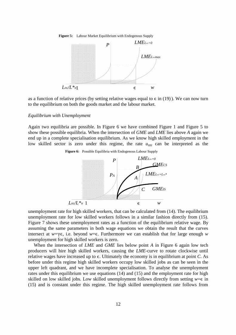
Figure 5: Labour Market Equilibrium with Endogenous Supply

Figure 6: Possible Equilibria with Endogenous Labour Supply

as a function of relative prices (by setting relative wages equal to � in (19) ). We can now turn

to the equilibrium on both the goods market and the labour market.

Equilibrium with Unemployment

Again two equilibria are possible. In Figure 6 we have combined Figure 1 and Figure 5 toshow these possible equilibria. When the intersection of GME and LME lies above A again weend up in a complete specialisation equilibrium. As we know high skilled employment in thelow skilled sector is zero under this regime, the rate u can be interpreted as theHH

unemployment rate for high skilled workers, that can be calculated from (14). The equilibriumunemployment rate for low skilled workers follows in a similar fashion directly from (15).Figure 7 shows these unemployment rates as a function of the equilibrium relative wage. Byassuming the same parameters in both wage equations we obtain the result that the curvesintersect at w=��, i.e. beyond w=�. Furthermore we can establish that for large enough wunemployment for high skilled workers is zero.

When the intersection of LME and GME lies below point A in Figure 6 again low techproducers will hire high skilled workers, causing the LME-curve to rotate clockwise untilrelative wages have increased up to �. Ultimately the economy is in equilibrium at point C. Asbefore under this regime high skilled workers occupy low skilled jobs as can be seen in theupper left quadrant, and we have incomplete specialisation. To analyse the unemploymentrates under this equilibrium we use equations (14) and (15) and the employment rate for highskilled on low skilled jobs. Low skilled unemployment follows directly from setting w=� in(15) and is constant under this regime. The high skilled unemployment rate follows from

w�

uL,H

uL

uH

��

u*

1

��(1-u*)^-5

P

uL,H

uH

1

PA

uHH

uL

eHHeHH

The figure can be extended beyond P , then it will be analogous to Figure 7.10A

13

Figure 7: Unemployment for High and Low Skilled Labour underComplete Specialisation

Figure 8: Unemployment for High and Low Skilled Labour underIncomplete Specialisation

subtracting the employed mismatch, obtained by setting w=� in (19), from the suppliedmismatch u under w=�. The latter is a constant and since the former is a decreasing functionHH

of relative prices - cf. the function e in Figure 8 - we can analyse the equilibriumHH

unemployment rates in P,u-space. Figure 8 presents both unemployment rates underincomplete specialisation . We do not consider the possibility that u is negative (low skilled10

H

producers cannot find high skilled workers to meet their demand) for this would only occurwhen the low tech product range is extremely large and the low skilled labour force isextremely small relative to the high skilled product range and labour force respectively.

In Figure 6 we show that compared to the incomplete specialisation equilibrium wageshave diverged under complete specialisation. By the convexity of the LME-curve, however,we also know that wages have not diverged as much as in the model with exogenous labour

supply. Relative unemployment rates might or might not have diverged between theseregimes. Figure 7 shows unemployment rates move in favour of high skilled workers as wagesdiverge. Hence we may conclude unemployment rates can indeed be traded off against wagedivergence under this regime. It depends on the parameters of the model where most of theadjustment to equilibrium arises. In the next section we will turn to the comparative statics ofthe model, when we allow for technical change.

14

4. Comparative Statics; Introducing Technical Change

In this section we introduce technical change into the model to see how it may explain theempirical evidence referred to in the introduction. First we define technical change in ourmodel as the expansion of either range of product varieties. Increasing the total range ofvarieties implies introducing new products into the economy, which we label product inno-vation.

These new products are both in terms of utility and production technology perfectlysymmetric to the already existing products in the range n . By our assumption of love ofH

variety, consumers will respond to the introduction of these new products by keeping theiraverage consumption of all products in the n range constant given the relative prices.H

However, these prices might change since the production of the additional new goods requiresthe allocation of high skilled labour to the new firms and hence high skilled wages will tend toincrease. Since relative prices are a mark up over relative wages by equation (9) this causesrelative prices to increase as well.

There may, however, be a reserve of high skilled labour in low skilled jobs. The highskilled labour will be attracted by the higher relative wage. This inflow can offset the upwardpressure on wages in the high skilled sector and create an upward pressure in the low skilledlabour market. Hence relative wages can remain stable when the movement of high skilledlabour can offset the initial shock. Both high and low skilled wages rise proportionally undersuch an adjustment.

When such a reserve of mismatched labour is unavailable or insufficient to absorb theshock, high skilled wages will increase relative to low skilled wages and hence relative pricesrise as well. This causes consumers to reduce their average consumption of high tech productsand increase the average consumption of low tech products. As a consequence marginalproductivity moves in favour of high skilled workers, which brings relative marginalproductivity in line with the higher relative wages.

The other type of technical change we can distinguish is the development of processes andinterfaces that allow low skilled workers to produce products that required high skills before.We label these process innovations. In our model this implies an increase in the range n and aL

corresponding decrease in n . In our model this will cause exactly the opposite of the above.H

Consumers will keep the average consumption of products in the range n constant givenL

relative prices and hence the demand for low skilled efficiency units increases. When thereexists a positive mismatch at the outset, relative wages are at �. Hence low tech producers cancompete for additional high skilled labour in the high skilled labour market. This implies anoutflow of high skilled labour from the high skilled sector that puts an upward pressure onhigh skilled wages as well. A new equilibrium is reached when enough high skilled labour hasmoved to low skilled jobs to produce the additional output. Wages again rise in proportionand hence relative wages remain stable (at �) as do relative prices.

LHL/L*H w

P

�

LME

A

B

C

A’

C’

LME’

We assume for now the adjustment to equilibrium does not cause the relative price to fall below the11

critical relative price level for which no further high skilled employment can be attracted by the lowsector producers at a relative wage �.

The latter, provided C lies above w=�.�.12

15

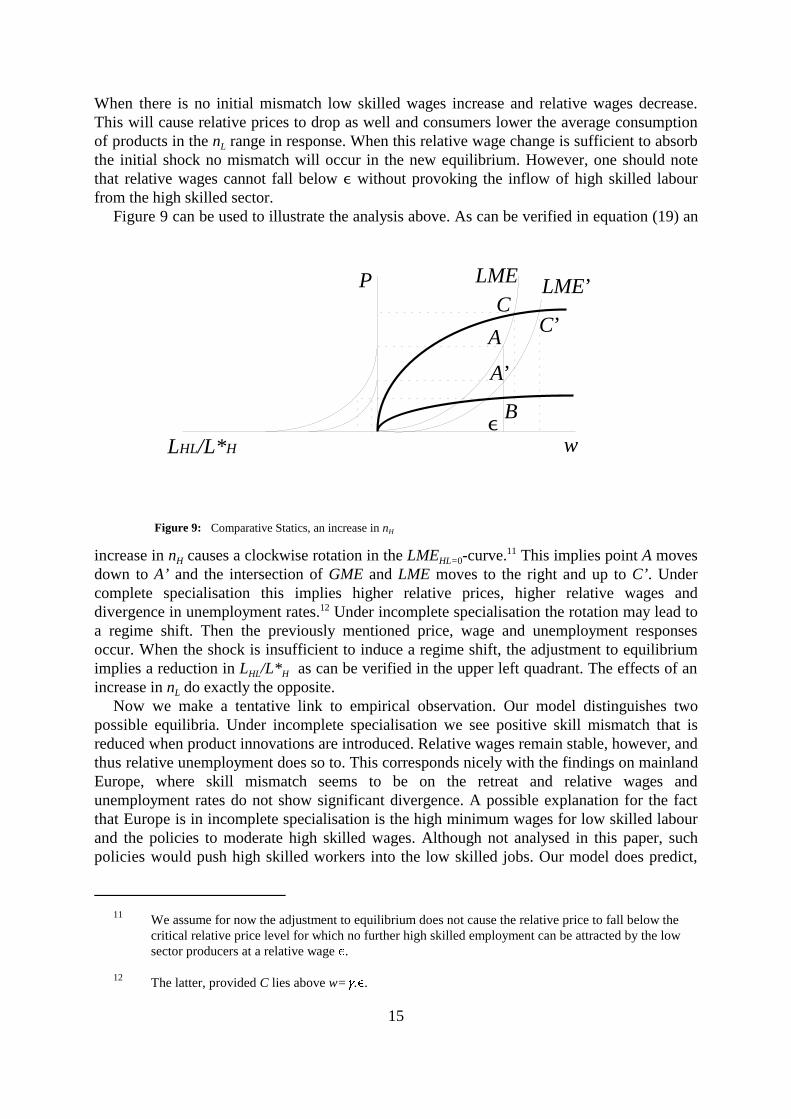
Figure 9: Comparative Statics, an increase in nH

When there is no initial mismatch low skilled wages increase and relative wages decrease.This will cause relative prices to drop as well and consumers lower the average consumptionof products in the n range in response. When this relative wage change is sufficient to absorbL

the initial shock no mismatch will occur in the new equilibrium. However, one should notethat relative wages cannot fall below � without provoking the inflow of high skilled labourfrom the high skilled sector.

Figure 9 can be used to illustrate the analysis above. As can be verified in equation (19) an

increase in n causes a clockwise rotation in the LME -curve. This implies point A movesH HL=011

down to A’ and the intersection of GME and LME moves to the right and up to C’. Undercomplete specialisation this implies higher relative prices, higher relative wages anddivergence in unemployment rates. Under incomplete specialisation the rotation may lead to12

a regime shift. Then the previously mentioned price, wage and unemployment responsesoccur. When the shock is insufficient to induce a regime shift, the adjustment to equilibriumimplies a reduction in L /L* as can be verified in the upper left quadrant. The effects of anHL H

increase in n do exactly the opposite.L

Now we make a tentative link to empirical observation. Our model distinguishes twopossible equilibria. Under incomplete specialisation we see positive skill mismatch that isreduced when product innovations are introduced. Relative wages remain stable, however, andthus relative unemployment does so to. This corresponds nicely with the findings on mainlandEurope, where skill mismatch seems to be on the retreat and relative wages andunemployment rates do not show significant divergence. A possible explanation for the factthat Europe is in incomplete specialisation is the high minimum wages for low skilled labourand the policies to moderate high skilled wages. Although not analysed in this paper, suchpolicies would push high skilled workers into the low skilled jobs. Our model does predict,

16

however, that this stability of relative wages and unemployment will not last as the skillintensive sector expands.

Under complete specialisation our model predicts that increases in the range of skillintensive goods will cause wage divergence and divergence of unemployment rates. Mismatchis absent in this regime. This situation might apply to the United States, the United Kingdomand most countries in the British Commonwealth. In these countries mismatch is apparentlynot considered a big problem since hardly any attention is devoted to it in economic literature.Wage divergence and real wage decreases for low skilled workers, however, is al the moreimportant and Nickell and Bell (1995) show biases in labour demand account for a large partof the asymmetry in unemployment in these countries counter to Krugman’s analysis.

5. Conclusions

In this paper we have presented a model that generates two possible equilibria. Using thecharacteristics of these equilibria we can identify the regime of incomplete specialisation withmainland Europe whereas the Anglo-Saxon world seems to be completely specialised. Thisimplies that both will respond differently to similar technological shocks.

A surge in the development of new products, that remains to be shown over the lastdecades but can certainly not be dismissed beforehand, can explain wage divergence andincreasing asymmetries in unemployment in the Anglo-Saxon world whereas it also causes adecrease in skill mismatch in mainland Europe. We do acknowledge there are many moredifferences between and within these area’s of the OECD and do not intend to explain all ofthe differences in labour market performance solely from this point of view. We do, however,contend that biased technical change can be a common cause without causing the sameeffects.

Furthermore our analysis sheds a different light on the policies implemented in the area’sdistinguished above. Relying on the so called chimney-effect to improve labour marketperspectives for low skilled workers in Europe will eventually be self-defeating as completespecialisation is achieved. The undesirable side effects of such a regime are to be consideredin formulating such policies. Policies of wage moderation do improve the situation for lowskilled workers but imply welfare losses due to inefficient allocation of skills.

As to the US policy of promoting technical change and R&D to create jobs for theunskilled, this may actually backfire. promoting R&D in general may increase thedevelopment and introduction of new products and cause an aggravation of the problem.Technology policy cannot, however, be evaluated without introducing an explicit R&D sectorinto the model. we therefore put this at the top of our research agenda. For now we suffice byconcluding the R&D policy should be targeted in order to deal with the problem ofasymmetric unemployment and wage divergence.

w�!/ ![1��] 1 1u�

1uHH

UHwL[w�] LHH [1u�]L �

H!

LHHnHlL ew

1

1��

LHH [1u�]

1 ![1�/w]

1��

L �

H

For simplicity we assume that unemployment benefits are equal to the wage that would have been13

earned when working, minus benefits from leisure. Therefore being unemployed is not a threat in thebargaining process.

Equation (A3) can also be written as:14

which is very similar to (14).

17

(A1)

(A2)

(A3)

Annex: Alternative for the wage formation process

The aim of this Annex is to present a wage formation process which is different from theprocess presented in the text above, but none-the-less yields a LME-curve with similarproperties. This intends to illustrate the rather general nature of our analysis.

Assume that both high and low skilled wages are set by unions in a context of a right-to-manage model That is, wages are set such that the utility of the union is maximised given theimplications for demand for labour- cf. equations (9') and (10).

The union that represents high skilled workers is assumed to desire the highest possiblewage for it’s members, but this wage must always exceed the low skilled wage by some factor�>1 to compensate for the costs of acquiring the higher skills. Hence w=w /w >�, should holdH L

at all times. Moreover, high skilled employment is valued with an intensity ! relative to13

wages and we assume, some minimum acceptable level of employment, defined as a share of the “natural”employment level (1-u*)L *. The union utility function is thus given by:H

The equilibrium demand for labour can be expressed as a function of relative wages bycombining (9) and (10), which yields:

The union is assumed to take the average employment level in the other sector as given.Hence maximising utility with respect to relative wages subject to the demand for labour inequation (A2) yields:14

ULwH[1��]w1LL [1u�]L �

L!

LLnLlHHw1

1��

LL [1u�]

1 !

1��

L �

L

LHH

LL e

[1u�]

1��![1�/w]L �

H

[1u�]

1��!L �

L��[1��]LHL

Taking the parameters u*, � and 5 for both bargaining processes is just for convenience and does not15

alter the qualitative results.

However, the low-skilled workers ignore the potential presence of high-skilled workers on low skilled16

jobs.

18

(A4)

(A5)

(A6)

(A7)

Preferences for the union representing the low skilled workers similarly express a desire for ahighest possible wage, which must exceed their outside option, the unemployment benefit, w ,u

by at least a factor � to compensate them for the leisure lost. Hence w -�w > 0 at all times.15L u

Assuming unemployment benefits are a constant fraction � of low skilled wages, substituingfor unemployment benefits and multiplying and dividing by the high skilled wage yields theexcess of low skilled wages over their minimum acceptable wage as w (1-��)w . Like in theH

-1

case of the union for high skilled labour we assume the union for low skilled labour also caresfor employment. Moreover we assume for simplicity employment enters the union utility16

function in the same way as for the high skilled workers union:

Again we find the equilibrium demand for labour from combining (9') and (10):

Since the low skilled union takes the level of high skilled wages and average high skilledemployment as exogenous, maximising the utility function with respect to relative wagesgiven labour demand yields:

Finally we assume that in equilibrium L =L +�L holds, hence employers in the low skilledLe L HL

sector are assumed to be indifferent between high or low skilled labour, measured inefficiency units. Combining equations (A3) and (A6) yields the relative aggregate supply oflabour:

LHH

LL e

nH

nL

wP

1�1

PwnL

nH

1� [1u�]

1��![1�/w]L �

H

[1u�]

1��!L �

L��[1��]LHL

1�

19

(A8)

(A9)

Confronting this expression with the aggregate version of (10):

yields the LME-curve:

It can be shown that LME-curve essentially has the same properties as the LME-curve in (19).Both the first and second derivative with respect to w are positive under our parameterrestrictions, implying the LME-curve is upward sloping and convex in P,w-space. The analysisthen can be pursued along the lines after equation (19) in the text.

20

References

Agenor P.R. and J. Aizenman (1996), ‘Wage Dispersion and Technical Progress’, in: NBERWorking Papers Series, No. 5417 CBS (1995), Enquete Beroepsbevolking 1995, The Hague, the Netherlands

Berman, E., J. Bound and Z. Grilliches (1994), Changes in the Demand for Skilled Labor inUS Manufacturing; Evidence from the Annual Survey of Manufactures’, in: QuarterlyJournal of Economics, Vol. CIX, No. 2, 367-397

Binswanger, H. (1974a),’A Microeconomic Approach to Induced Innovation’, in: TheEconomic Journal, 84, 940-957

Binswanger, H. (1974b),’The Measurement of Biased Technical Change with many Factors ofProduction’, in: American Economic Review, 64, No. 5, 964-976

Brauer, D. and S. Hickok (1995),’Explaining the Growing Inequality in Wages across SkillLevels’, in: Economic Policy Review, Federal Reserve Bank of New York, 1 (January), 61-72

Burtless, G (1994),’International Trade and the Rise in Earnings Inequality’, Journal ofEconomic Perspectives, 33 (June), 800-816

Draper, N. and T. Manders (1997), ‘Structural Changes in the Demand for Labour, in: DeEconomist, 145 (4), 521-546

Feenstra, R. and G. Hanson (1997), ‘Productivity Measurement and the Impact of Trade andTechnology on Wages: Estimates for the U.S., 19972-1990', in: NBER Working Paper Series,No. 6052

Groot, W. and H. Maassen van den Brink (1996), ‘Overscholing en Verdringing op deArbeidsmarkt’, in: Economisch Statistiche Berichten, 74 (7), 74-77 Halaby, C. (1994), ‘Overeducation and Skill Mismatch’, in: Sociology of Education, 67, 47-59

Howell, D. (1995),’Collapsing Wages and Rising Inequality: Has Computerisation Shifted theDemand for Skills?’,Challenge, 38 (1), 27-35

Jackman, R. (1995), Unemployment and Wage Inequality in OECD Countries, London Schoolof Economics, Oxford University Press

Kennedy, P. (1964), ‘Induced Bias in Innovation and the Theory of Distribution’, in: TheEconomic Journal, 74, no. 295, 541-547

Koopmans , M. and C. Teulings (1987),’Verdringing op de Arbeidsmarkt’, in: EconomischStatistische Berichten, 72, 592-595

21

Krugman, P. (1979), ‘A Model of Innovation, Technology Transfer and the WorldDistribution of Income’, in: Journal of Political Economy, 87 (2), 253-265

Krugman, P. (1995), ‘Technology, Trade and Factor Prices’, in: NBER Working Paper Series,No. 5355

Lawrence, R. Z. and M. J. Slaughter (1993), ‘International Trade and American Wages in the1980s’, in: Brookings Papers in Economic Activity, 2 (April), 161-210

Layard, R. and S. J. Nickell (1992), Unemployment in the OECD Countries, London Schoolof Economics, Oxford University Press

Leamer, E. (1994), ‘Trade, Wages and Revolving Doors Ideas’, in: NBER Working PapersSeries, No. 4716

Leamer, E. (1995),’A Trade Economist’s View of US Wages and Globalization’, in: Collins,ed. (1995), Imports, Exports and the American Worker, Washington: Brookings

Muysken, J. and B. Ter Weel (1998), ‘Overeducation and Crowding Out of Low-SkilledWorkers’, MERIT Research Memorandum 98-023, Maastricht University, Maastricht

Nickell, S. and B. Bell (1995),’The Collapse in Demand for the Unskilled and Unemploymentacross the OECD’, in: Oxford Review of Economic Policy, 11 (1), 40-62

OECD (1994), Jobs Study, Evidence and Explanations, Part I; Labour Market Trends andUnderlying Forces of Change, OECD, Paris

Phelps and Dandrakis (1966),’A Model of Induced Invention, Growth and Distribution’, in:the Economic Journal, 76, no. 304, 823-840

Salter, W. (1960), Productivity and Technical Change, Cambridge

Teulings and Hartog, (1998), Corporatism or competition?, Cambridge University Press, UK

Zon van A., H. Meijers and J. Muysken (1998), ‘Sweeping the Chimney before kindling theFire as a Workable option for Employment Policy’, in: MERIT Research Memorandum, 2/98-016, MERIT, Maastricht