walch education - dr. d. dambreville's math page -...
TRANSCRIPT


1 2 3 4 5 6 7 8 9 10
ISBN 978-0-8251-7377-6
Copyright © 2014
J. Weston Walch, Publisher
Portland, ME 04103
www.walch.com
Printed in the United States of America
EDUCATIONWALCH
These materials may not be reproduced for any purpose.The reproduction of any part for an entire school or school system is strictly prohibited.
No part of this publication may be transmitted, stored, or recorded in any formwithout written permission from the publisher.

iiiTable of Contents
Introduction . . . . . . . . . . . . . . . . . . . . . . . . . . . . . . . . . . . . . . . . . . . . . . . . . . . . . . . . . . . . . . v
Unit 6: Mathematical ModelingLesson 1: Creating Equations . . . . . . . . . . . . . . . . . . . . . . . . . . . . . . . . . . . . . . . . . . . . U6-1Lesson 2: Piecewise, Step, and Absolute Value Functions . . . . . . . . . . . . . . . . . . . U6-76Lesson 3: Working with Constraint Equations and Inequalities . . . . . . . . . . . . . U6-115Lesson 4: Transformations of Graphs . . . . . . . . . . . . . . . . . . . . . . . . . . . . . . . . . . . U6-157Lesson 5: Comparing Properties Within and Between Functions . . . . . . . . . . . U6-183Lesson 6: Operating on Functions . . . . . . . . . . . . . . . . . . . . . . . . . . . . . . . . . . . . . . U6-240Lesson 7: Inverses of Functions . . . . . . . . . . . . . . . . . . . . . . . . . . . . . . . . . . . . . . . . U6-266Lesson 8: Geometric Modeling. . . . . . . . . . . . . . . . . . . . . . . . . . . . . . . . . . . . . . . . . U6-310
Answer Key . . . . . . . . . . . . . . . . . . . . . . . . . . . . . . . . . . . . . . . . . . . . . . . . . . . . . . . . . . . . . AK-1
Table of Contents


vIntroduction
Welcome to the CCGPS Advanced Algebra Student Resource Book. This book will help you learn how to use algebra, geometry, data analysis, and probability to solve problems. Each lesson builds on what you have already learned. As you participate in classroom activities and use this book, you will master important concepts that will help to prepare you for the EOCT and for other mathematics assessments and courses.
This book is your resource as you work your way through the Advanced Algebra course. It includes explanations of the concepts you will learn in class; math vocabulary and definitions; formulas and rules; and exercises so you can practice the math you are learning. Most of your assignments will come from your teacher, but this book will allow you to review what was covered in class, including terms, formulas, and procedures.
• In Unit 1: Inferences and Conclusions from Data, you will learn about summarizing and interpreting data and using the normal curve. You will explore populations, random samples, and sampling methods, as well as surveys, experiments, and observational studies. Finally, you will compare treatments and read reports.
• In Unit 2: Polynomial Functions, you will begin by exploring polynomial structures and operations with polynomials. Then you will go on to prove identities, graph polynomial functions, solve systems of equations with polynomials, and work with geometric series.
• In Unit 3: Rational and Radical Relationships, you will be introduced to operating with rational expressions. Then you will learn about solving rational and radical equations and graphing rational functions. You will solve and graph radical functions. Finally, you will compare properties of functions.
• In Unit 4: Exponential and Logarithmic Functions, you will start working with exponential functions and begin exploring logarithmic functions. Then you will solve exponential equations using logarithms.
• In Unit 5: Trigonometric Functions, you will begin by exploring radians and the unit circle. You will graph trigonometric functions, including sine and cosine functions, and use them to model periodic phenomena. Finally, you will learn about the Pythagorean Identity.
Introduction

Introductionvi
• In Unit 6: Mathematical Modeling, you will use mathematics to model equations and piecewise, step, and absolute value functions. Then, you will explore constraint equations and inequalities. You will go on to model transformations of graphs and compare properties within and between functions. You will model operating on functions and the inverses of functions. Finally, you will learn about geometric modeling.
Each lesson is made up of short sections that explain important concepts, including some completed examples. Each of these sections is followed by a few problems to help you practice what you have learned. The “Words to Know” section at the beginning of each lesson includes important terms introduced in that lesson.
As you move through your Advanced Algebra course, you will become a more confident and skilled mathematician. We hope this book will serve as a useful resource as you learn.
Lesson 1: Creating EquationsUNIT 6 • MATHEMATICAL MODELING
U6-1Lesson 1: Creating Equations
6.1
Common Core Georgia Performance Standards
MCC9–12.A.CED.1★
MCC9–12.A.CED.2★
MCC9–12.F.IF.4★
MCC9–12.F.IF.5★
MCC9–12.F.IF.7a★
MCC9–12.F.IF.7b★
MCC9–12.F.IF.7c★
MCC9–12.F.IF.7d★ (+)
MCC9–12.F.IF.7e★
MCC9–12.F.IF.8a
MCC9–12.F.IF.8b
MCC9–12.F.BF.1a★
Essential Questions
1. How does the behavior of a linear function differ from that of a quadratic function?
2. How are asymptotes used to describe the end behavior of data?
3. What is meant by inverse properties of exponential and logarithmic functions?
4. What do the periodicity and amplitude of a trigonometric function reveal about the function?
WORDS TO KNOW
asymptote a line that a function gets closer and closer to, but never crosses or touches
axis of symmetry of a parabola
the line through the vertex of a parabola about which
the parabola is symmetric. The equation of the axis of
symmetry is 2
=−xb
a.
base the quantity that is being raised to a power in an exponential expression; in ax, a is the base
constraint a limit or restriction on the domain, range, and/or solutions of a mathematical or real-world problem

U6-2Unit 6: Mathematical Modeling 6.1
data fitting the process of assigning a rule, usually an equation or formula, to a collection of data points as a method of predicting the values of new dependent variables that result from new independent-variable values
domain the set of all input values (x-values) that satisfy the given function without restriction
e an irrational number with an approximate value of 2.71828; e is the base of the natural logarithm (ln x or loge x)
exponential equation an equation of the form y = abx, where x is the independent variable, y is the dependent variable, and a and b are real numbers
exponential function a function in the form f(x) = a(bx) + c, where a, b, and c are constants and b is greater than 0 but not equal to 1
extrema the minima or maxima of a function
half plane a region containing all points that has one boundary, a line or curve that continues in both directions infinitely. The line or curve may or may not be included in the region. A half plane can be used to represent a solution to an inequality statement.
hole a point on the graph of a function representing where the function is undefined; a point on the graph at which the function is not connected
inequality a mathematical statement that compares the value of an expression in one independent variable to the value of a dependent variable using the comparison symbols >, <, ≥, and ≤
interval a set of values between a lower bound and an upper bound
linear equation an equation that can be written in the form ax + by = c, where a, b, and c are constants; can also be written as y = mx + b, in which m is the slope and b is the y-intercept. The graph of a linear equation is a straight line; its solutions are the infinite set of points on the line.

U6-3Lesson 1: Creating Equations
6.1
logarithmic equation an equation of the form y = loga x, which is an inverse of the exponential equation y = ax if x > 0. Given an exponential equation of the form x = by, the logarithmic equation is y = logb x, where y is the exponent, b is the base, and x is the argument.
maximum the greatest value or highest point of a function
minimum the least value or lowest point of a function
natural exponential function
an exponential function with a base of e
natural logarithm a logarithm whose base is the irrational number e; usually written in the form “ln,” which means “loge”
parent function a function with a simple algebraic rule that represents a family of functions. The graphs of the functions in the family have the same general shape as the parent function.
polynomial equation an equation of the general form = + + + + +−
−1
12
21 0y a x a x a x a x an
nn
n , where a1 is a rational number, an ≠ 0, and n is a nonnegative integer and the highest degree of the polynomial
quadratic equation an equation that can be written in the form y = ax2 + bx + c, where x is the independent variable, y is the dependent variable, a, b, and c are constants, and a ≠ 0
range the set of all outputs of a function; the set of y-values that are valid for the function
root the x-intercept of a function; also known as zero
symmetrical having two parts that are mirror images when reflected over a line or rotated around a point
symmetry of a function the property whereby a function exhibits the same behavior (e.g., graph shape, function values) for specific domain values and their opposites
vertex of a parabola the point on a parabola that is the maximum or minimum
zero the x-intercept of a function; also known as root
U6-4Unit 6: Mathematical Modeling 6.1
Recommended Resources
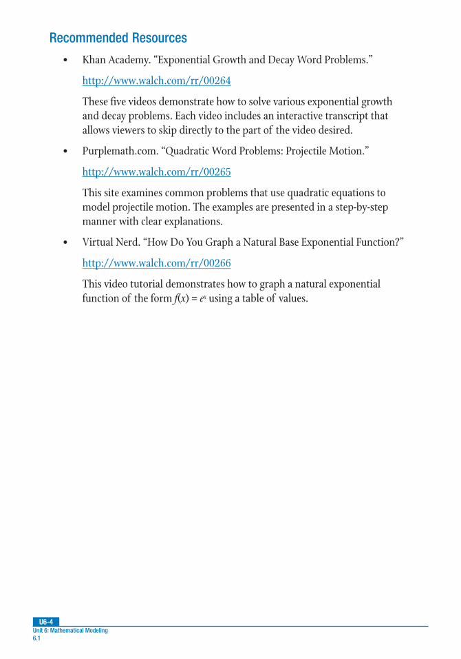
• Khan Academy. “Exponential Growth and Decay Word Problems.”
http://www.walch.com/rr/00264
These five videos demonstrate how to solve various exponential growth and decay problems. Each video includes an interactive transcript that allows viewers to skip directly to the part of the video desired.
• Purplemath.com. “Quadratic Word Problems: Projectile Motion.”
http://www.walch.com/rr/00265
This site examines common problems that use quadratic equations to model projectile motion. The examples are presented in a step-by-step manner with clear explanations.
• Virtual Nerd. “How Do You Graph a Natural Base Exponential Function?”
http://www.walch.com/rr/00266
This video tutorial demonstrates how to graph a natural exponential function of the form f(x) = ex using a table of values.

U6-5Lesson 1: Creating Equations
6.1.1
IntroductionOften, the solutions to equations in real-world situations depend on a single variable. For example, if you are selling lollipops for $1 each for a prom fund-raiser, the amount of money you raise depends only on how many lollipops you sell. Creating equations in one variable to describe a mathematical or real-world situation typically requires analyzing data or viewing a visual display of the data, such as a graph on a coordinate plane. Sometimes you may need to analyze both the data and a visual display of the information.
Key Concepts
• An independent variable, labeled on the x-axis, is the quantity that changes based on values chosen. It is also referred to as the input variable of an equation or function.
• A dependent variable, labeled on the y-axis, is the quantity that changes based on the input values of the independent variable. The dependent variable is often referred to as the output variable of an equation or function.
• Mathematically, the number of data points needed to create an equation in one variable depends on the type of function that is being created.
• A data point (or ordered pair) is a point (x, y) on a two-dimensional coordinate plane that represents the value of an independent variable (x) that results in a specific dependent variable value (y).
• Data points also result from solutions for an equation or inequality in one variable that originate from a real-world situation.
• Recall that an inequality is a mathematical statement that compares the value of an expression in one independent variable to the value of a dependent variable using the comparison symbols >, <, ≥, and ≤.
• The data points or ordered pairs that make the inequality a true statement are the solutions of the inequality statement.
• Recall that a linear equation is an equation that can be written in the form ax + by = c, where a, b, and c are constants, or y = mx + b, in which m is the slope and b is the y-intercept. The graph of a linear equation is a straight line, and its solutions are the infinite set of points on the line.
• Only two data points are needed to write a linear equation in one variable because the graph of a linear equation is a straight line that is determined by two points. Therefore, the x- and y-intercepts and the slope of a straight line can be found using only two data points.
Lesson 6.1.1: Creating Equations in One Variable
U6-6Unit 6: Mathematical Modeling 6.1.1
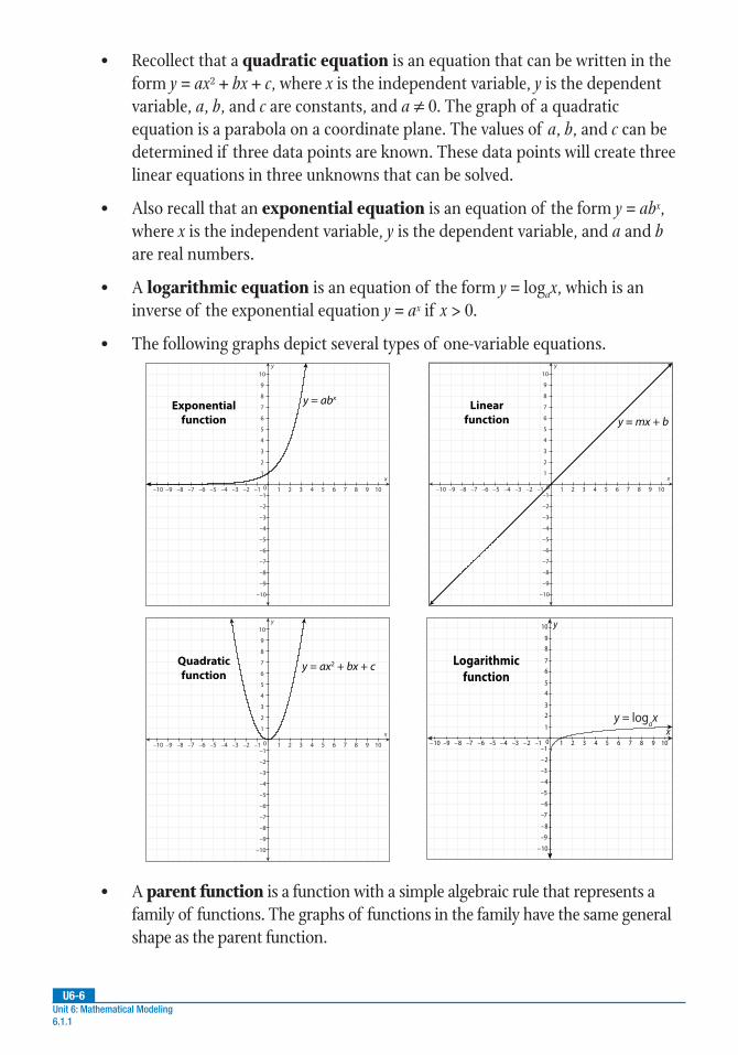
• Recollect that a quadratic equation is an equation that can be written in the form y = ax2 + bx + c, where x is the independent variable, y is the dependent variable, a, b, and c are constants, and a ≠ 0. The graph of a quadratic equation is a parabola on a coordinate plane. The values of a, b, and c can be determined if three data points are known. These data points will create three linear equations in three unknowns that can be solved.
• Also recall that an exponential equation is an equation of the form y = abx, where x is the independent variable, y is the dependent variable, and a and b are real numbers.
• A logarithmic equation is an equation of the form y = logax, which is an inverse of the exponential equation y = ax if x > 0.
• The following graphs depict several types of one-variable equations.
–10 –9 –8 –7 –6 –5 –4 –3 –2 –1 0 1 2 3 4 5 6 7 8 9 10
–10
–9
–8
–7
–6
–5
–4
–3
–2
–1
1
2
3
4
5
6
7
8
9
10
y = abxExponentialfunction
–10 –9 –8 –7 –6 –5 –4 –3 –2 –1 0 1 2 3 4 5 6 7 8 9 10
–10
–9
–8
–7
–6
–5
–4
–3
–2
–1
1
2
3
4
5
6
7
8
9
10
y = mx + bLinearfunction
–10 –9 –8 –7 –6 –5 –4 –3 –2 –1 0 1 2 3 4 5 6 7 8 9 10
–10
–9
–8
–7
–6
–5
–4
–3
–2
–1
1
2
3
4
5
6
7
8
9
10
y = ax2 + bx + cQuadraticfunction
–10 –8 –6 –4 –2 2 4 6 8 1097531–1–3–5–7–9
x
10
9
7
5
3
1
8
6
4
2
0
–2
–4
–6
–8
–10
y
–1
–3
–5
–7
–9
y = logax
Logarithmicfunction
• A parent function is a function with a simple algebraic rule that represents a family of functions. The graphs of functions in the family have the same general shape as the parent function.

U6-7Lesson 1: Creating Equations
6.1.1
• When analyzing the graph of an equation or function, it is important to consider the mathematical constraints on the graph. Constraints are limits or restrictions on the domain, range, and/or solutions of a mathematical or real-world problem. Constraints can result from mathematical and real-world considerations. Recall that the domain is the set of all input values (x-values) that satisfy the given equation or function without restriction, and the range is the set of all outputs (y-values) that are valid for the equation or function.
• Later in the lesson, real-world constraints will be applied to one-variable equations and their parent functions.
• Formulas can be useful in determining how variables relate to one another. Formally, a formula is a mathematical statement of the relationship between two or more variables. The variables’ values are sometimes constrained by mathematical or real-world conditions.
• An inequality in one variable can be written for exponential, linear, logarithmic, and quadratic equations in one variable. The solutions to the inequality are defined as the set of data points or ordered pairs that make the inequality true in the half plane of a coordinate plane.
• A half plane is a region containing all points on one side of a boundary, which is a line or curve that continues in both directions infinitely. The line or curve may or may not be included in the region. A half plane can be used to represent a solution to an inequality statement.
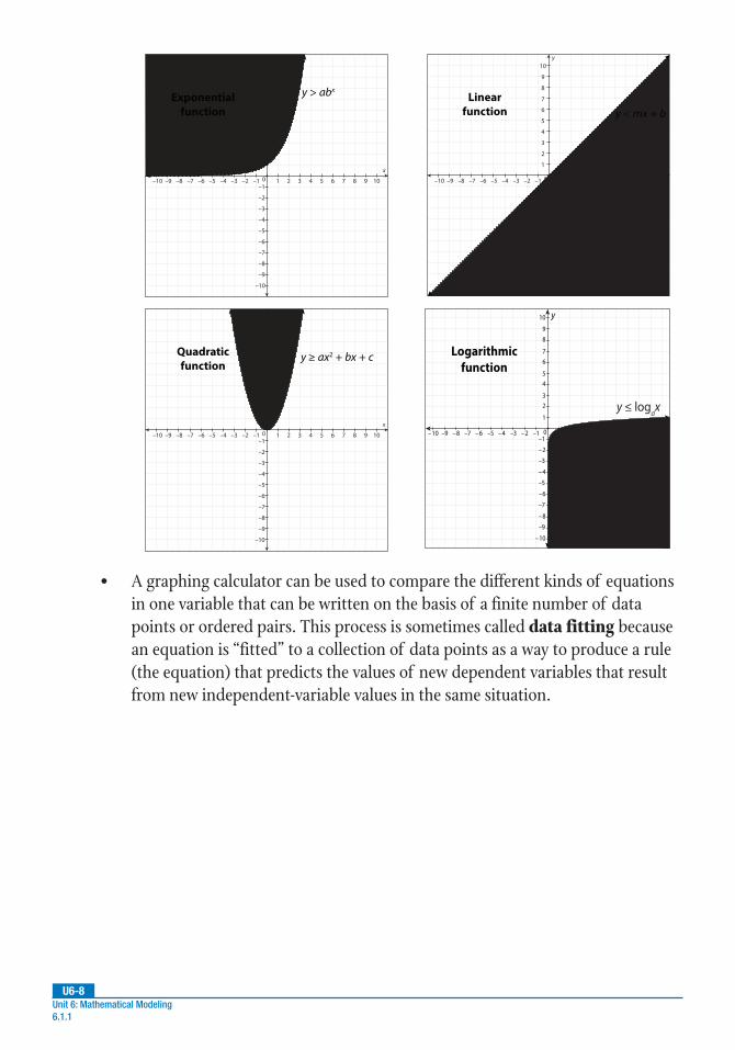
• A half plane is used to represent a linear inequality of the form ax + by > c instead of the straight line that represents a linear equation of the form ax + by = c. (The linear inequality would be y > mx + b for a linear equation in slope-intercept form, y = mx + b.) In fact, the straight line and the half plane together represent the mathematical solutions possible for the inequality. In this case, the straight line is a boundary for the half plane and does not include the points on the line in the solution for the inequality. The inequality is greater than (>), not greater than or equal to (≥). The graphs that follow show the one-variable equations from the previous graphs, now changed to inequalities that use the four different types of inequality conditions (>, <, ≥, and ≤).
U6-8Unit 6: Mathematical Modeling 6.1.1
–10 –9 –8 –7 –6 –5 –4 –3 –2 –1 0 1 2 3 4 5 6 7 8 9 10
–10
–9
–8
–7
–6
–5
–4
–3
–2
–1
1
2
3
4
5
6
7
8
9
10
y > abxExponentialfunction
–10 –9 –8 –7 –6 –5 –4 –3 –2 –1 0 1 2 3 4 5 6 7 8 9 10
–10
–9
–8
–7
–6
–5
–4
–3
–2
–1
1
2
3
4
5
6
7
8
9
10
Linearfunction y < mx + b
–10 –9 –8 –7 –6 –5 –4 –3 –2 –1 0 1 2 3 4 5 6 7 8 9 10
–10
–9
–8
–7
–6
–5
–4
–3
–2
–1
1
2
3
4
5
6
7
8
9
10
y ≥ ax2 + bx + cQuadraticfunction
–10 –8 –6 –4 –2 2 4 6 8 1097531–1–3–5–7–9
x
10
9
7
5
3
1
8
6
4
2
0
–2
–4
–6
–8
–10
y
–1
–3
–5
–7
–9
y ≤ logax
Logarithmicfunction
• A graphing calculator can be used to compare the different kinds of equations in one variable that can be written on the basis of a finite number of data points or ordered pairs. This process is sometimes called data fitting because an equation is “fitted” to a collection of data points as a way to produce a rule (the equation) that predicts the values of new dependent variables that result from new independent-variable values in the same situation.

U6-9Lesson 1: Creating Equations
6.1.1
• To fit an equation to the graph of a set of data points, follow the directions appropriate to your calculator model. Either calculator will return values for the constants that can be substituted into the equation y = ax + b or y = ax2 + bx + c, depending on the type of equation chosen. These values can be verified by calculating the slope and y-intercept of a line passing through the points.
On a TI-83/84:
Step 1: Press [STAT] to bring up the statistics menu. The first option, 1: Edit, will already be highlighted. Press [ENTER].
Step 2: Arrow up to L1 and press [CLEAR], then [ENTER], to clear the list. Repeat this process to clear L2 as needed.
Step 3: From L1, press the down arrow to move your cursor into the list. Enter the x-value of the first ordered pair. Press [ENTER]. Repeat until all x-values have been entered.
Step 4: Press the right arrow key and enter the y-value of the first ordered pair next to its x-value. Press [ENTER]. Repeat until all y-values have been entered.
Step 5: Press [2ND][Y=] to bring up the STAT PLOTS menu.
Step 6: The first option, Plot 1, will already be highlighted. Press [ENTER].
Step 7: Under Plot 1, select ON if it isn’t selected already.
Step 8: Arrow over to Plot 2 and repeat. Check that “Xlist:” is set to “L1” and “Ylist:” is set to “L2.” Press [ENTER] to save any changes.
Step 9: Press [ZOOM] and select 6: ZStandard to produce a four-quadrant grid. Notice the graphed data points.
Step 10: To fit an equation to the data points, press [STAT] and arrow over to the CALC menu. Then, select 4: LinReg(ax+b) or 5: QuadReg, depending on the type of graph desired.
Step 11: Press [2ND][1] to type “L1” for Xlist. Arrow down to Ylist and press [2ND][2] to type “L2” for Ylist, if not already shown.
Step 12: Arrow down to “Calculate” and press [ENTER].

U6-10Unit 6: Mathematical Modeling 6.1.1
On a TI-Nspire:
Step 1: Press the [home] key. Arrow over to the spreadsheet icon, the fourth icon from the left, and press [enter].
Step 2: To clear the lists in your calculator, arrow up to the topmost cell of the table to highlight the entire column, then press [menu]. Choose 3: Data, then 4: Clear Data. Repeat for each column as necessary.
Step 3: Arrow up to the topmost cell of the first column, labeled “A.” Press [X][enter] to type x. Then, arrow over to the second column, labeled “B.” Press [Y][enter] to type y.
Step 4: Arrow down to cell A1 and enter the first x-value. Press [enter]. Enter the second x-value in cell A2 and so on.
Step 5: Move over to cell B1 and enter the first y-value. Press [enter]. Enter the second y-value in cell B2 and so on.
Step 6: To see a graph of the points, press the [home] key. Arrow over to the graphing icon, the second icon from the left, and press [enter]. Press [menu], then select 3: Graph Type, and 4: Scatter Plot.
Step 7: At the bottom of the screen, use the pop-up menus to enter “x” for the x-variable and “y” for the y-variable. Press [enter]. The data points are displayed.
Step 8: If needed, adjust the viewing window. Press [menu], then select 4: Window/Zoom, and then 1: Window Settings. Change the settings as appropriate.
Step 9: To fit an equation to the data points, first press [ctrl] and the up arrow key to display the open windows. Highlight the table of x- and y-values and press [enter]. Press [menu] and select 4: Statistics, and then 1: Stat Calculations. Select the desired type of equation from the list. The coefficients of the desired equation will be listed in a table.
• Note: A word of caution is needed in using a graphing calculator to fit a quadratic equation based on given data. The generated equation is of the “best fit,” which means that it may not exactly fit the data points. In real-world problems, such approximations are a result of using inexact or sometimes unreliable measurements or measuring tools.

U6-11Lesson 1: Creating Equations
6.1.1
Guided Practice 6.1.1Example 1
Aaron wants to have his company’s logo printed on tablet computer cases, so that he can give away the cases as part of a marketing campaign. A specialty printing company will charge Aaron a $750 fee to design and print the personalized cases, plus the cost of the actual cases. The price of each case is $3. How many personalized cases can Aaron purchase if his budget is $1,200?
1. Write an equation in words for determining the total cost to produce the personalized cases.
Review the problem statement to determine the given information and the information that is needed to solve the problem.
The total cost of buying the cases includes a fee plus the cost of the actual cases.
The cost of the cases is determined by the price of each case multiplied by the number of cases.
Summarize this information as an equation in words:
The total cost is the fee plus the price of each case multiplied by the number of cases.
2. Write an equation for the cost for n cases.
Let C represent the cost of the cases.
The cost, C, of n cases is equal to C(n).
From the problem statement, we know that n cases will cost $3 each.
We also know that the fee is $750.
In the word equation written for step 1, substitute C(n) for the total cost, $750 for the fee, n for the number of cases, and $3 for the price of each case:
total cost
is fee plusprice of
each casemultiplied
bynumber of cases
↓ ↓ ↓ ↓ ↓ ↓ ↓C(n) = $750 + $3 • n
The mathematical equation for the cost, C, of n cases is C(n) = 750 + 3n.

U6-12Unit 6: Mathematical Modeling 6.1.1
3. Determine how much money Aaron will have left to spend on cases after paying the fee.
Aaron’s budget is $1,200. Subtract the fee of $750 from the amount Aaron has to spend.
1200 – 750 = 450
After the fee, Aaron has $450 to spend on cases.
4. Determine the number of cases Aaron can buy.
Aaron has $450 to spend on cases and the price of each case is $3. Therefore, divide $450 by $3 to determine the number of cases he can afford.
450
3150=
Aaron can buy 150 cases.
5. Use the equation to check the result.
Check the result by substituting 1,200 for C(n) and 150 for n in the equation determined in step 2.
C(n) = 750 + 3n Equation determined in step 2
(1200) = 750 + 3(150) Substitute 1,200 for C(n) and 150 for n.
1200 = 750 + 450 Multiply.
1200 = 1200 Add.
The answer results in a true statement. Aaron can buy 150 cases with his budget of $1,200.
U6-13Lesson 1: Creating Equations
6.1.1
Example 2
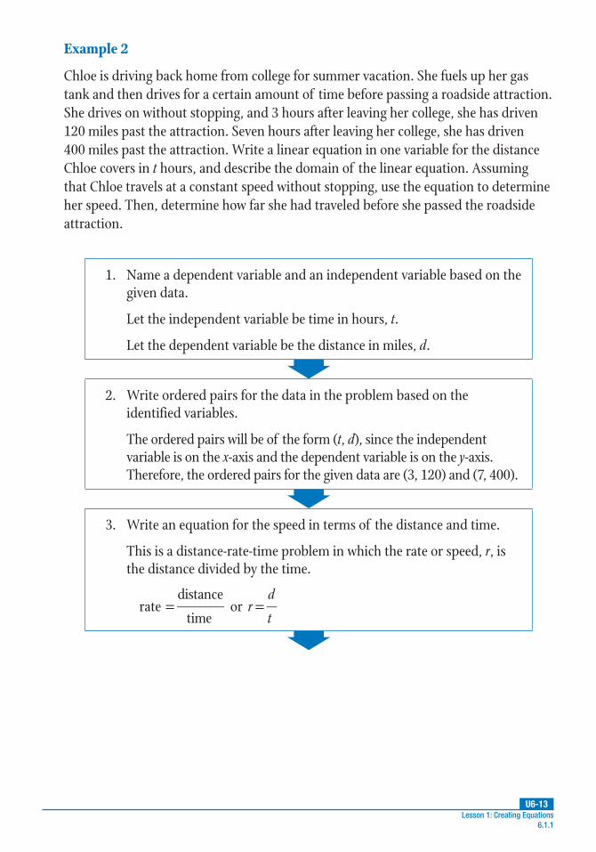
Chloe is driving back home from college for summer vacation. She fuels up her gas tank and then drives for a certain amount of time before passing a roadside attraction. She drives on without stopping, and 3 hours after leaving her college, she has driven 120 miles past the attraction. Seven hours after leaving her college, she has driven 400 miles past the attraction. Write a linear equation in one variable for the distance Chloe covers in t hours, and describe the domain of the linear equation. Assuming that Chloe travels at a constant speed without stopping, use the equation to determine her speed. Then, determine how far she had traveled before she passed the roadside attraction.
1. Name a dependent variable and an independent variable based on the given data.
Let the independent variable be time in hours, t.
Let the dependent variable be the distance in miles, d.
2. Write ordered pairs for the data in the problem based on the identified variables.
The ordered pairs will be of the form (t, d), since the independent variable is on the x-axis and the dependent variable is on the y-axis. Therefore, the ordered pairs for the given data are (3, 120) and (7, 400).
3. Write an equation for the speed in terms of the distance and time.
This is a distance-rate-time problem in which the rate or speed, r, is the distance divided by the time.
ratedistance
time= or r
d
t=

U6-14Unit 6: Mathematical Modeling 6.1.1
4. Use the two ordered pairs from step 2 and the formula for the slope of
a one-variable equation, my y
x x2 1
2 1
=−−
, to find the rate.
The slope formula can be used to find the rate because it is of the
same form as the formula rd
t= .
Recall that the two-point slope formula is my y
x x2 1
2 1
=−−
for points (x1, y1)
and (x2, y2). We can think of this as rd d
t t2 1
2 1
=−−
for points (t1, d1) and
(t2, d2). Thus, the slope m would also be the rate r at which Chloe drives.
Let (3, 120) represent (t1, d1) and (7, 400) represent (t2, d2).
Substitute these values into the formula for slope.
rd d
t t2 1
2 1
=−−
Slope formula written in terms of the rate, r
r(400) (120)
(7) (3)=
−−
Substitute (3, 120) for (t1, d1) and (7, 400) for (t2, d2).
r280
4= Simplify.
r = 70
Chloe’s speed during her 7-hour drive was 70 miles per hour.

U6-15Lesson 1: Creating Equations
6.1.1
5. Use the point-slope formula, y – y1 = m(x – x1), to write the linear equation in one variable.
In the point-slope formula, y – y1 = m(x – x1), m is the slope and (x1, y1) is a point on the line. Use the value r = 70 from the previous step for the slope and either of the given ordered pairs for (x1, y1) in this formula.
Let’s use (3, 120). Simplify and solve for d.
y – y1 = m(x – x1) Point-slope formula
(d) – (120) = (70)[(t) – (3)]Substitute (3, 120) for (x1, y1), d for y, r for m, and t for x.
d – 120 = 70t – 210 Distribute.
d = 70t – 90 Simplify.
6. Find the value of d when t = 0.
t = 0 represents the time at which Chloe left college for the drive home.
d = 70t – 90 Equation from the previous step
d = 70(0) – 90 Substitute 0 for t.
d = –90 Simplify.
When t = 0, d = –90.
7. Interpret the results based on the information given in the problem to determine how far Chloe drove before passing the roadside attraction.
If Chloe drove at a constant speed of 70 miles per hour, the ordered pair (3, 120) implies that she had traveled 3 • 70 or 210 miles from her starting point. The distance 120 in the ordered pair implies that Chloe was 210 – 120 or 90 miles past that starting point when she passed the roadside attraction. Therefore, Chloe drove 90 miles before passing the roadside attraction.

U6-16Unit 6: Mathematical Modeling 6.1.1
Example 3
Write a quadratic equation in one variable that is true for the three data points (0, 0), (1, 2), and (2, 8) by solving a system of three equations based on the standard form of a quadratic equation, y = ax2 + bx + c. Then, use your equation to find the y-value for a fourth point on the same graph that has an x-value of 3.
1. Use the given data points to write three equations using the standard form of a quadratic equation.
Substitute the x- and y-values from each of the three data points into y = ax2 + bx + c and simplify.
For (0, 0): For (1, 2): For (2, 8):y = ax2 + bx + c y = ax2 + bx + c y = ax2 + bx + c(0) = a(0)2 + b(0) + c (2) = a(1)2 + b(1) + c (8) = a(2)2 + b(2) + cc = 0 2 = a + b + c 8 = 4a + 2b + c
Substitute c = 0 into the other two equations to produce two equations in two unknowns.
For (1, 2): For (2, 8):2 = a + b + c 8 = 4a + 2b + c2 = a + b + (0) 8 = 4a + 2b + (0)2 = a + b 8 = 4a + 2b
4 = 2a + b
We now have two separate equations. We must continue to simplify until only one equation that is true for all three given points remains.

U6-17Lesson 1: Creating Equations
6.1.1
2. Examine the resulting equations for any common traits that can be used to simplify them.
Compare 2 = a + b to 4 = 2a + b.
Notice that the constants in both equations are multiples of 2.
Make the left sides of the two equations equal by multiplying the terms in the first equation by 2.
2 = a + b
2 • 2 = 2 • (a + b)
4 = 2a + 2b
3. Use the results to solve for another variable.
Set the right sides of the two equations equal to each other and solve for any variable possible in order to eliminate another variable from the system of equations.
4 = 2a + 2b Revised first equation
4 = 2a + b Second equation
Set the right sides equal and solve.
2a + 2b = 2a + b
2b – b = 2a – 2a
b = 0
Substitute the value found for b into either of the equations 4 = 2a + 2b or 4 = 2a + b. This will allow the value of the third variable to be found.
Solve for a in 4 = 2a + b by substituting 0 for b.
4 = 2a + b
4 = 2a + (0)
4 = 2a
a = 2
U6-18Unit 6: Mathematical Modeling 6.1.1
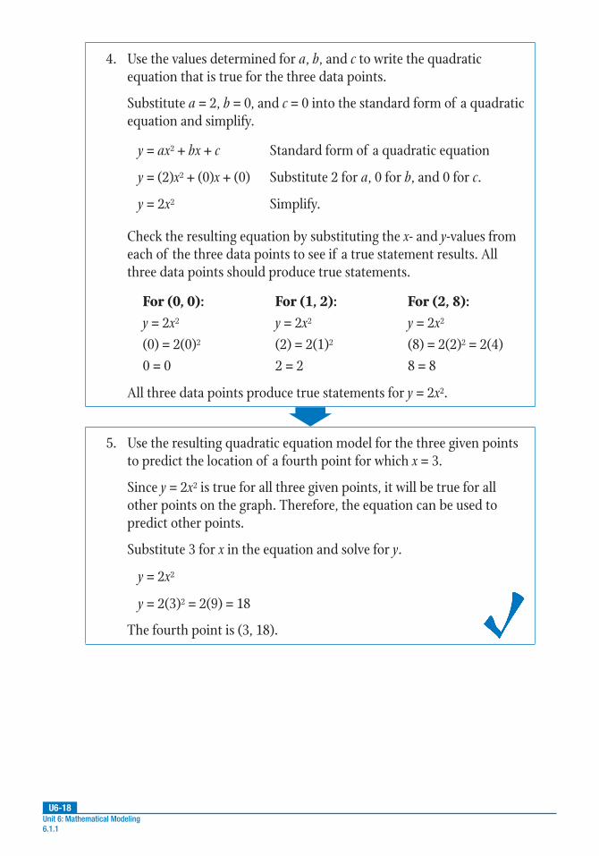
4. Use the values determined for a, b, and c to write the quadratic equation that is true for the three data points.
Substitute a = 2, b = 0, and c = 0 into the standard form of a quadratic equation and simplify.
y = ax2 + bx + c Standard form of a quadratic equation
y = (2)x2 + (0)x + (0) Substitute 2 for a, 0 for b, and 0 for c.
y = 2x2 Simplify.
Check the resulting equation by substituting the x- and y-values from each of the three data points to see if a true statement results. All three data points should produce true statements.
For (0, 0): For (1, 2): For (2, 8):y = 2x2 y = 2x2 y = 2x2
(0) = 2(0)2 (2) = 2(1)2 (8) = 2(2)2 = 2(4)0 = 0 2 = 2 8 = 8
All three data points produce true statements for y = 2x2.
5. Use the resulting quadratic equation model for the three given points to predict the location of a fourth point for which x = 3.
Since y = 2x2 is true for all three given points, it will be true for all other points on the graph. Therefore, the equation can be used to predict other points.
Substitute 3 for x in the equation and solve for y.
y = 2x2
y = 2(3)2 = 2(9) = 18
The fourth point is (3, 18).

U6-19Lesson 1: Creating Equations
6.1.1
Example 4
The data shows the current i in milliamps (mA) in a cell phone circuit in fractions of a second after a cell-tower signal is received.
Time, t (s) 0.1 0.2 0.3 0.4 0.5 0.6 0.7 0.8 0.9Current, i (mA) 2 3 5 8 13 21 34 55 89
Graph these points on a graphing calculator. Use the graph to write an exponential equation of the general form y = abx that approximately fits the data. Then, rewrite the resulting equation so that it includes a power of 10.
1. Name an independent variable and a dependent variable.
In this case, the current increases as a function of the elapsed time.
Dependent variable: i (current in milliamps)
Independent variable: t (time in seconds)
2. Use the table of values to determine the data points.
Follow the format (t, i), using the convention that the independent variable is listed first.
The data points are (0.1, 2), (0.2, 3), (0.3, 5), (0.4, 8), (0.5, 13), (0.6, 21), (0.7, 34), (0.8, 55), and (0.9, 89).

U6-20Unit 6: Mathematical Modeling 6.1.1
3. Plot the points on a graphing calculator and use the graph to find the exponential function for the data.
The graph of the points will allow you to estimate values for the constants a and b in the general form y = abx. With these values, you can write an equation that approximately fits the given data.
On a TI-83/84:
Step 1: Press [STAT] to bring up the statistics menu. The first option, 1: Edit, will already be highlighted. Press [ENTER].
Step 2: Arrow up to L1 and press [CLEAR], then [ENTER], to clear the list. Repeat this process to clear L2 as needed.
Step 3: From L1, press the down arrow to move your cursor into the list. Enter the t-value of the first ordered pair. Press [ENTER]. Repeat until all t-values have been entered.
Step 4: Press the right arrow key and enter the i-value of the first ordered pair next to its t-value. Press [ENTER]. Repeat until all i-values have been entered.
Step 5: Press [2ND][Y=] to bring up the STAT PLOTS menu.
Step 6: The first option, Plot 1, will already be highlighted. Press [ENTER].
Step 7: Under Plot 1, select ON if it isn’t selected already.
Step 8: Arrow over to Plot 2 and repeat. Check that “Xlist:” is set to “L1” and “Ylist:” is set to “L2.” Press [ENTER] to save any changes.
Step 9: Press [WINDOW] to set the viewing window to display the data: Xmin = 0, Xmax = 1, Xscl = 0.1, Ymin = 0, Ymax = 90, Yscl = 10.
Step 10: Press [GRAPH] to see the data graph.
Step 11: To fit an equation to the data points, press [STAT] and arrow over to the CALC menu. Then, select 0: ExpReg.
Step 12: Press [2ND][1] to type “L1” for Xlist. Arrow down to Ylist and press [2ND][2] to type “L2” for Ylist, if not already shown.
Step 13: Arrow down to “Calculate” and press [ENTER]. The resulting equation is of the general form y = abx, in which a and b are constants.
(continued)
U6-21Lesson 1: Creating Equations
6.1.1
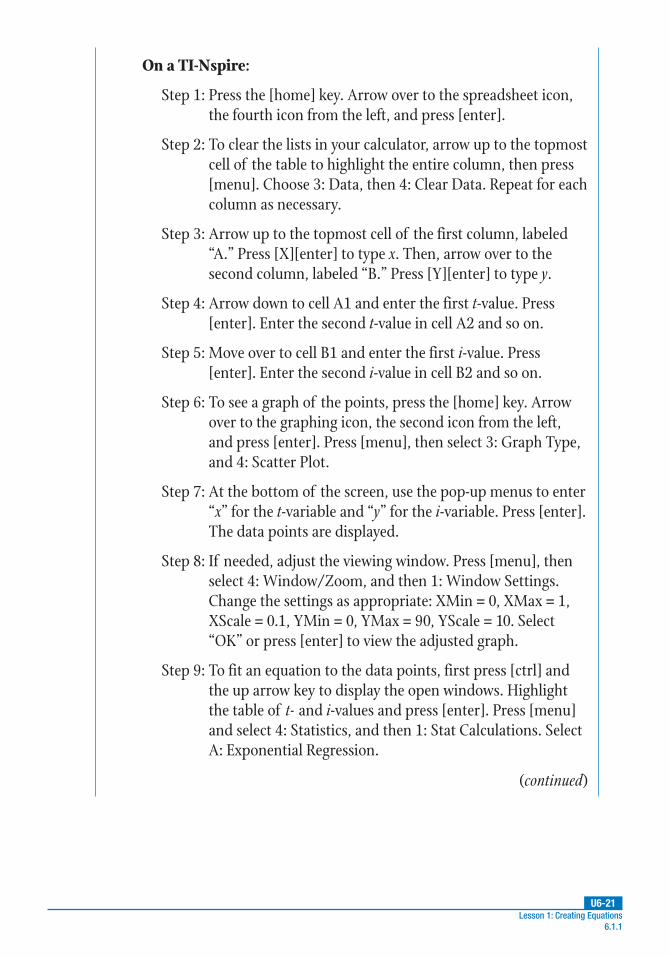
On a TI-Nspire:
Step 1: Press the [home] key. Arrow over to the spreadsheet icon, the fourth icon from the left, and press [enter].
Step 2: To clear the lists in your calculator, arrow up to the topmost cell of the table to highlight the entire column, then press [menu]. Choose 3: Data, then 4: Clear Data. Repeat for each column as necessary.
Step 3: Arrow up to the topmost cell of the first column, labeled “A.” Press [X][enter] to type x. Then, arrow over to the second column, labeled “B.” Press [Y][enter] to type y.
Step 4: Arrow down to cell A1 and enter the first t-value. Press [enter]. Enter the second t-value in cell A2 and so on.
Step 5: Move over to cell B1 and enter the first i-value. Press [enter]. Enter the second i-value in cell B2 and so on.
Step 6: To see a graph of the points, press the [home] key. Arrow over to the graphing icon, the second icon from the left, and press [enter]. Press [menu], then select 3: Graph Type, and 4: Scatter Plot.
Step 7: At the bottom of the screen, use the pop-up menus to enter “x” for the t-variable and “y” for the i-variable. Press [enter]. The data points are displayed.
Step 8: If needed, adjust the viewing window. Press [menu], then select 4: Window/Zoom, and then 1: Window Settings. Change the settings as appropriate: XMin = 0, XMax = 1, XScale = 0.1, YMin = 0, YMax = 90, YScale = 10. Select “OK” or press [enter] to view the adjusted graph.
Step 9: To fit an equation to the data points, first press [ctrl] and the up arrow key to display the open windows. Highlight the table of t- and i-values and press [enter]. Press [menu] and select 4: Statistics, and then 1: Stat Calculations. Select A: Exponential Regression.
(continued)

U6-22Unit 6: Mathematical Modeling 6.1.1
Step 10: At the “Exponential Regression” settings screen, use the pop-up menus to select “x” for X List and “y” for Y List. Press [enter]. The coefficients in the quadratic equation y = abx should be listed in the table with the data points.
Either calculator will return approximate results for a and b of a ≈ 1.2 and b ≈ 120. Substituting these values into the general form y = abx results in the equation y = 1.2 • 120x. Note that this is an equation of best fit, since the constants are approximate.
4. Rewrite the base to include a power of 10.
The base of the exponent variable can be rewritten as a power of 10, and then simplified using the properties of exponents.
y = 1.2 • 120x Equation from the previous step
y = 1.2 • (1.2 •102)x Rewrite 120 as a power of 10.
y = 1.2 • (1.2)x • (10)2x Apply the Power of Powers Property.
y = 1.2x + 1 • 102x Rewrite using the Product of Powers Property.
The exponential equation written in base 10 that fits the data in the table is y = 1.2x + 1 • 102x.

U6-23
PRACTICE
UNIT 6 • MATHEMATICAL MODELINGLesson 1: Creating Equations
Lesson 1: Creating Equations 6.1.1
For problems 1–3, write an equation in one variable that fits the data points exactly without using a calculator.
1. (–2, –3), (1, 2), and (3, 4)
2. 1,2
3−
, (0, 2), and (1, 6)
3. (–5, 2), (1, 2), and (4, 2)
For problems 4–7, write an equation in one variable in the simplest form of the equation type listed, using all three of the graphed data points.
–2 –1.5 –1 –0.5 0.5 1 1.5 2
x
3
2.5
2
1.5
1
0.5
0
–0.5
–1
y
4. an exponential equation
5. a linear equation
6. a logarithmic equation
7. a quadratic equation
Practice 6.1.1: Creating Equations in One Variable
continued

U6-24
PRACTICE
UNIT 6 • MATHEMATICAL MODELINGLesson 1: Creating Equations
Unit 6: Mathematical Modeling 6.1.1
Read the scenario that follows, and use the information in it to complete problems 8–10.
Darien rode her bike from a starting point (0, 0) at a speed that constantly changed according to the equation d(t) = –5t2 + 35t, in which d is the distance in miles and t is the time in hours. After 2 hours, Darien had traveled 50 miles. Her friend Jaceylo biked from the same starting point (0, 0) for 1 hour at a speed of 30 miles per hour. Then, Jaceylo biked at a different speed for another hour. Jaceylo followed the same route as Darien and ended up at the same destination.
8. Write a linear equation to represent the first hour of Jaceylo’s bike ride.
9. Write a linear equation to represent the second hour of Jaceylo’s bike ride.
10. At what speed was Jaceylo traveling over the second hour?

U6-25Lesson 1: Creating Equations
6.1.2
Introduction
Linear equations are ideal for modeling any situation that involves a quantity that is changing at a constant rate. While linear equations are appropriate for some situations, they may be inadequate for situations that involve other rates of change. For instance, if you add a certain amount of money to a piggy bank at regular intervals, your savings will increase at a constant rate. However, if you move your money to a bank savings account that pays compounding interest, your savings will increase exponentially. In this case, an exponential model is better for showing the faster growth rate. The type of equation that is chosen depends on the situation. Sometimes, a graph can be more effective in seeing patterns and in solving problems. There are similarities and differences between the equations and graphs of linear, exponential, quadratic, and polynomial functions that can be observed when solving a variety of problems.
Key Concepts
• Recall that functions and equations can both be written in the form “y =.” Generally, functions are written in the form “f(x) =,” but “y =” is also commonly used.
Linear Functions and Equations
• Linear functions and equations are used to model a rate of change that is constant.
• Recall that linear equations can be written in the form ax + by = c, where a, b, and c are constants. They can also be written as y = mx + b, in which m is the slope and b is the y-intercept.
• The degree of a linear function or equation (i.e., the exponent) is equal to 1.
• The graph of a linear equation or function is a line.
Exponential Functions and Equations
• An exponential function or equation is appropriate to use when the rate of change increases or decreases very rapidly, but not at a constant rate.
• Recall that an exponential equation is an equation of the form y = abx, where x is the independent variable, y is the dependent variable, and a and b are real numbers.
Lesson 6.1.2: Creating Equations in Two Variables

U6-26Unit 6: Mathematical Modeling 6.1.2
• An exponential function is a function in the form f(x) = a(bx) + c, where a, b, and c are constants and b is greater than 0 but not equal to 1.
• In the simpler exponential form f(x) = bx, where b is a real number, b is the base, or the quantity being raised to the power or exponent x.
• The graph of an exponential function is a curved line.
• In the following graph of the exponential function f(x) = 2x, the left side of the curve (to the left of the y-axis) approaches the x-axis but never touches it, whereas the right side of the curve (to the right of the y-axis) increases rapidly as the x-values approach positive infinity.
16
14
12
10
8
6
4
2
0
– 2
– 15 – 10 – 5 5
y
x
f(x) = 2x
• In this example, the x-axis is an asymptote, or a line that a function gets closer and closer to, but never crosses or touches. Asymptotes can be horizontal (located at y = a, where a is a real number) or vertical (at x = a, where a is a real number).
• An exponential equation that includes a variable in the exponent can be solved for that variable by using logarithms to rewrite the equation. Given an exponential equation of the form x = by, the logarithmic equation is y = logb x, where y is the exponent, b is the base, and x is the argument. Note that this logarithmic form is an equivalent rewriting of the exponential form.

U6-27Lesson 1: Creating Equations
6.1.2
• The resulting equation can be solved by taking the log, which is an operation that can be computed by hand or on a calculator.
• Recall that logarithms can also be used to find the inverse of an exponential equation. For example, given an exponential equation y = ax with x > 0, the equivalent logarithmic form is x = loga y, but the inverse is y = loga x. Notice that x and y have been switched because this is an inverse.
Quadratic Functions and Equations
• A quadratic function or equation can be used to model a rate of change that increases and then decreases (or decreases and then increases).
• A quadratic equation is an equation that can be written in the form y = ax2 + bx + c, where x is the independent variable, y is the dependent variable, a, b, and c are constants, and a ≠ 0.
• In a quadratic function, the maximum is the greatest value or highest point, and the minimum is the least value or lowest point. The maximum is the point at which an increasing rate of change begins to decrease; the minimum is where a decreasing rate of change begins to increase.
• The U-shaped graph of a quadratic function is called a parabola. The vertex of a parabola is the minimum or maximum point of a parabola.
• The parabola will have symmetry on either side of the vertex point. A parabola that is symmetrical has two parts that are mirror images when reflected over a line or rotated around a point. That is, each half of the parabola will be exactly the same size and shape but reversed on either side of the vertex.
• The symmetry of a function is the property whereby a function exhibits the same behavior (e.g., graph shape, function values) for specific domain values and their opposites.

U6-28Unit 6: Mathematical Modeling 6.1.2
• The axis of symmetry of a parabola is the line through the vertex of
the parabola about which the parabola is symmetric. For instance, in the
following graph of the function f(x) = x2, the y-axis runs through the center
of the parabola and is the axis of symmetry of the parabola. For a parabola
in standard form, or y = ax2 + bx + c, the equation of the axis of symmetry is
=−2
xb
a. All parabolas have an axis of symmetry.
16
14
12
10
8
6
4
2
0
–2
–15 –10 –5 5
y
x
f(x) = ax2
• For quadratics in the form of f(x) = ax2 + bx + c, the parabola crosses the x-axis at points called zeros. The zero or root is the x-intercept of the function, and is written in the form (0, a), where a is a real number. These roots or solutions are obtained by solving the quadratic equation.
• Most quadratics in the form ax2 + bx + c can be solved by factoring them into two binomials (x ± a)(x ± b) and then solving for x.
• Some quadratics can be solved by a technique called completing the square. This involves using mathematical manipulations on the original equation to convert it into a perfect square trinomial that can be factored into two binomials.
Polynomial Functions and Equations
• A polynomial equation or function consists of multiple terms (quantities separated by a plus or minus sign), in the general form = + + + + +−
−1
12
21 0y a x a x a x a x an
nn
n . In this form, a1 is a rational number, an ≠ 0, and n is a nonnegative integer and the highest degree of the polynomial. Note that the exponents of a polynomial function are never negative.

U6-29Lesson 1: Creating Equations
6.1.2
• Some polynomials are named by their highest degree, such as cubic (third-degree), or quartic (fourth-degree). It is customary to refer to a polynomial with a degree higher than 4 as a higher-order degree polynomial.
• Polynomials are useful in modeling rates of change that have increasing and decreasing behavior over intervals. An interval is a set of values between a lower bound and an upper bound. Sometimes a phenomenon is increasing over a specific interval, and sometimes it is decreasing over a specific interval.
• The graph of a polynomial is a curve that may contain multiple sections that rise to high points (maxima) and dip to low points (minima).
x
y
f(x)
Local minimum
Local maxima
0
• The highest point on the graph of a polynomial is the absolute maximum, while all other high points are called relative maxima. Formally, the relative maximum of a function is the greatest value for a particular interval of the function; it is sometimes referred to as a local maximum.
• Similarly, the lowest point on the graph of a polynomial is called the absolute minimum. Low points in a certain area of the curve are called relative minima. The relative minimum (or local minimum) is the least value for a particular interval of the function.
• The set of all maxima and minima for a polynomial curve are referred to as the extrema.
• You can identify maximum points by observing what happens to the curve before and after a point. For a maximum point, the curve will increase, reach the maximum point, and then decrease. For a minimum point, the curve will decrease, reach the minimum point, and then increase.
• A polynomial curve will cross the x-axis at its zeros. These can be found visually by graphing the function using technology and then estimating where the curve crosses the x-axis.

U6-30Unit 6: Mathematical Modeling 6.1.2
Guided Practice 6.1.2Example 1
A water fountain’s spout releases water into the fountain’s basin at a flow rate of 10 inches per second. The function d(x) = 4 + vx – 10x2 can be used to model this situation, where d is the distance (in inches) the water travels, v is the flow rate of the water, and x is the time in seconds. Rewrite the given function to model the flow rate of the water from the time it leaves the spout to the time it hits the basin. Then, create a graph of this function using a table of values. When is the graph increasing and decreasing? What is the maximum height of the water in the fountain?
1. Rewrite the function to reflect the given flow rate of the water.
The problem states that in the original function d(x) = 4 + vx – 10x2, v represents the speed of the water. The problem also states that the water travels at a speed of 10 inches per second. Therefore, substitute 10 for v.
d(x) = 4 + vx – 10x2 Original function
d(x) = 4 + (10)x – 10x2 Substitute 10 for v.
The function d(x) = 4 + 10x – 10x2 can be used to model the flow rate of the water.
2. Create a graph using a table of values to represent this scenario.
Begin by finding the vertex of the parabola. This will allow you to more efficiently choose values on either side of the parabola.
Recall that the x-value of the vertex is found using the formula for the
axis of symmetry, =−2
xb
a. To use this formula, write the quadratic
equation in standard form, ax2 + bx + c = 0.
d(x) = 4 + 10x – 10x2 written in standard form is –10x2 + 10x + 4 = 0; therefore, a = –10, b = 10, and c = 4.
=−2
xb
aVertex formula
=−−
(10)
2( 10)x Substitute –10 for a and 10 for b.
=1
2x Simplify.
The x-value of the vertex is 1
2.
(continued)
U6-31Lesson 1: Creating Equations
6.1.2
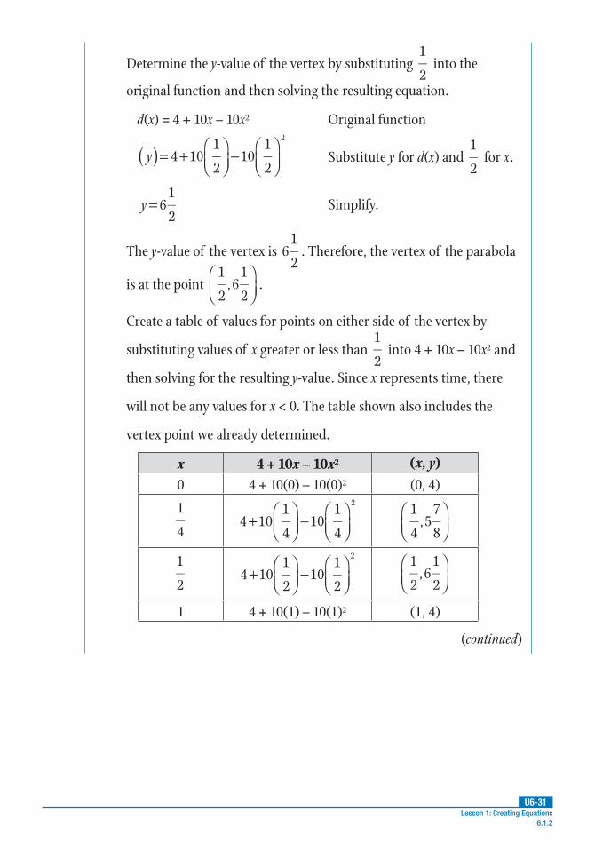
Determine the y-value of the vertex by substituting 1
2 into the
original function and then solving the resulting equation.
d(x) = 4 + 10x – 10x2 Original function
( )= +
−
4 101
210
1
2
2
y Substitute y for d(x) and 1
2 for x.
= 61
2y Simplify.
The y-value of the vertex is 61
2. Therefore, the vertex of the parabola
is at the point
1
2,6
1
2.
Create a table of values for points on either side of the vertex by
substituting values of x greater or less than 1
2 into 4 + 10x – 10x2 and
then solving for the resulting y-value. Since x represents time, there
will not be any values for x < 0. The table shown also includes the
vertex point we already determined.
x 4 + 10x – 10x2 (x, y)0 4 + 10(0) – 10(0)2 (0, 4)
1
4+
−
4 101
410
1
4
2
1
4,5
7
8
1
2 +
−
4 101
210
1
2
2
1
2,6
1
2
1 4 + 10(1) – 10(1)2 (1, 4)
(continued)

U6-32Unit 6: Mathematical Modeling 6.1.2
Sketch the values on a graph.
10
9
8
7
6
5
4
3
2
1
0 2 4 6 8 10
3. Determine when the graph is increasing and decreasing.
The graph of the parabola is increasing between x = 0 and =1
2x , and
decreasing for values of >1
2x .
4. Determine the maximum height of the water in the fountain.
The height of the water is represented by the y-values of the graph.
The maximum height of the water in the fountain occurs
at 61
2 inches.
U6-33Lesson 1: Creating Equations
6.1.2
Example 2
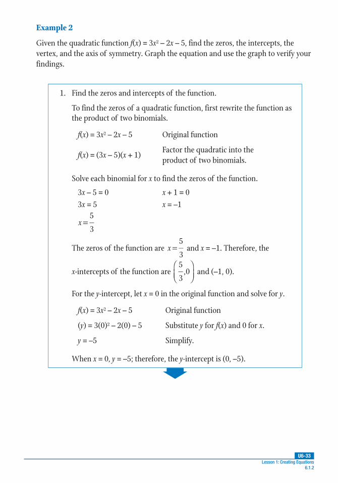
Given the quadratic function f(x) = 3x2 – 2x – 5, find the zeros, the intercepts, the vertex, and the axis of symmetry. Graph the equation and use the graph to verify your findings.
1. Find the zeros and intercepts of the function.
To find the zeros of a quadratic function, first rewrite the function as the product of two binomials.
f(x) = 3x2 – 2x – 5 Original function
f(x) = (3x – 5)(x + 1)Factor the quadratic into the product of two binomials.
Solve each binomial for x to find the zeros of the function.
3x – 5 = 0 x + 1 = 03x = 5 x = –1
=5
3x
The zeros of the function are =5
3x and x = –1. Therefore, the
x-intercepts of the function are
5
3,0 and (–1, 0).
For the y-intercept, let x = 0 in the original function and solve for y.
f(x) = 3x2 – 2x – 5 Original function
(y) = 3(0)2 – 2(0) – 5 Substitute y for f(x) and 0 for x.
y = –5 Simplify.
When x = 0, y = –5; therefore, the y-intercept is (0, –5).

U6-34Unit 6: Mathematical Modeling 6.1.2
2. Find the vertex and the axis of symmetry.
Finding the vertex of the parabola will allow you to more efficiently choose values on either side of the parabola.
Recall that the x-value of the vertex is found using the formula for the
axis of symmetry, =−2
xb
a.
To use this formula, make sure the quadratic is written in standard form, ax2 + bx + c = 0.
In standard form, 3x2 – 2x – 5 = 0, so a = 3, b = –2, and c = –5.
xb
a2= − Vertex formula
x( 2)
2(3)= −
−Substitute 3 for a and –2 for b.
x2
6= Simplify.
x1
3=
The x-value of the vertex is 1
3.
Determine the y-value of the vertex by substituting 1
3 into the
original function and then solving.
f(x) = 3x2 – 2x – 5 Original function
( )=
−
−3
1
32
1
35
2
y Substitute y for f(x) and 1
3 for x.
=−51
3y Simplify.
The y-value of the vertex is −51
3. Therefore, the vertex of the
parabola is at 1
3, 5
1
3−
.
The axis of symmetry is located at =1
3x .

U6-35Lesson 1: Creating Equations
6.1.2
3. Graph the function and use it to verify your findings.
Graph the function, either by hand or using a graphing calculator.
20
18
16
14
12
10
8
6
4
2
0– 2
– 4
– 6
– 8
– 10
– 10 – 5 5 10
y
x
As seen from the graph, the vertex does appear to be located at 1
3, 5
1
3−
, which is also the minimum of the function. It can also be
seen that the equation for the axis of symmetry is =1
3x . The graph of
the function crosses the x-axis at the points 5
3, 0
and (–1, 0), which
are the calculated zeros of the function.
Therefore, the graph verifies the results determined algebraically.

U6-36Unit 6: Mathematical Modeling 6.1.2
Example 3
Madelyn owns a small flower shop and is tallying up her expenses, which include the cost of flowers, wrapping paper, and other supplies, plus business fees for licenses, taxes, and rent. She figures the cost of selling x number of flowers includes a fixed cost of $2,750 in addition to $0.45 per flower sold. Write a cost function C(x) that models Madelyn’s business expenses. Create a table to analyze her costs for sales of 0, 500, 1,000, and 1,500 flowers. Use the table to sketch the graph of the function. What can you conclude about Madelyn’s costs at each sales level based on the shape of the graph?
1. Write a cost function C(x) that models Madelyn’s expenses.
Madelyn has a fixed cost of $2,750, plus a cost of $0.45 times the number of flowers sold, x. Using a linear function model, f(x) = mx + b, we can substitute the values 2750 and 0.45 from the problem to get C(x) = 0.45x + 2750. So, the cost of selling x number of flowers would be C(x) = 0.45x + 2750.
2. Use the cost function to create a table of values for the various flower sales.
The problem statement specified flower sales of 0, 500, 1,000, and 1,500, which represent different x-values.
Substitute these values into the cost function to find the corresponding ordered pairs.
x 0.45x + 2750 (x, C(x))0 0.45(0) + 2750 (0, 2750)
500 0.45(500) + 2750 (500, 2975)1000 0.45(1000) + 2750 (1000, 3200)1500 0.45(1500) + 2750 (1500, 3425)
U6-37Lesson 1: Creating Equations
6.1.2
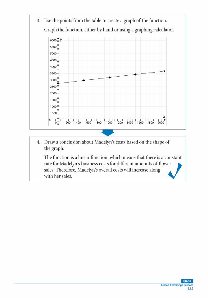
3. Use the points from the table to create a graph of the function.
Graph the function, either by hand or using a graphing calculator.
6000
5500
5000
4500
4000
3500
3000
2500
2000
1500
1000
500
0 200 400 600 800 1000 1200 1400 1600 1800 2000
y
x
4. Draw a conclusion about Madelyn’s costs based on the shape of the graph.
The function is a linear function, which means that there is a constant rate for Madelyn’s business costs for different amounts of flower sales. Therefore, Madelyn’s overall costs will increase along with her sales.
U6-38Unit 6: Mathematical Modeling 6.1.2
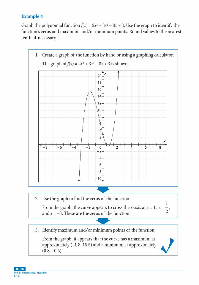
Example 4
Graph the polynomial function f(x) = 2x3 + 3x2 – 8x + 3. Use the graph to identify the function’s zeros and maximum and/or minimum points. Round values to the nearest tenth, if necessary.
1. Create a graph of the function by hand or using a graphing calculator.
The graph of f(x) = 2x3 + 3x2 – 8x + 3 is shown. 22
20
18
16
14
12
10
8
6
4
2
0– 2
– 4
– 6
– 8
– 10
– 8 – 6 – 4 – 2 2 4 6 8
y
x
2. Use the graph to find the zeros of the function.
From the graph, the curve appears to cross the x-axis at x = 1, =1
2x ,
and x = –3. These are the zeros of the function.
3. Identify maximum and/or minimum points of the function.
From the graph, it appears that the curve has a maximum at approximately (–1.8, 15.5) and a minimum at approximately (0.8, –0.5).

U6-39Lesson 1: Creating Equations
6.1.2
Example 5
Grayson owns an art gallery, and keeps track of how well each artist’s work sells each month. Grayson determines the sales of his top artist’s works can be modeled by the function f(x) = –0.0008x4 + 0.026x3 – 0.28x2 + 1.16x, where x is the number of months since the art pieces were unveiled, and f(x) is the number of art pieces sold in multiples of 10. Based on this function, how many pieces by Grayson’s top artist sold in 13 months? Which month had the highest sales of pieces by this artist? Grayson determined that the average sales model for the entire gallery over this same time period is g(x) = –0.0008x3 + 0.026x2 – 0.28x + 1.16. How do the top artist’s sales compare to the average number of sales for the whole gallery?
1. Determine the number of pieces by the top artist that sold in 13 months.
Substitute 13 for x, the number of months, and solve algebraically.
f(x) = –0.0008x4 + 0.026x3 – 0.28x2 + 1.16x
f(13) = –0.0008(13)4 + 0.026(13)3 – 0.28(13)2 + 1.16(13)
f(13) = –22.85 + 57.12 – 47.32 + 15.08
f(13) = 2.03
The function tracks sales of artworks in multiples of 10. Therefore, Grayson’s top artist sold 2.03 • 10, or approximately 20 pieces of art.

U6-40Unit 6: Mathematical Modeling 6.1.2
2. Graph the function by hand or using a calculator.
The graph of f(x) = –0.0008x4 + 0.026x3 – 0.28x2 + 1.16x is shown. The x-axis represents the number of months and the y-axis represents the number of pieces of art sold.
–10 –5 5 10 15 20 25 30
10
5
0
–5
–10
–15
–20
–25
–30
–35
–40
y
x
f(x)
3. Use the graph to determine the maximum.
The maximum represents the month in which the top artist sold the most pieces.
It can be seen from the graph that the maximum point occurs at month 13; therefore, the most sales from the top artist occurred during month 13, or about 1 year and 1 month after the art pieces were unveiled.
Compare the equation and graph of the top artist’s sales model to that of the gallery’s average sales model .
The equation that best models the sales for the gallery is g(x) = –0.0008x3 + 0.026x2 – 0.28x + 1.16.
(continued)
U6-41Lesson 1: Creating Equations
6.1.2
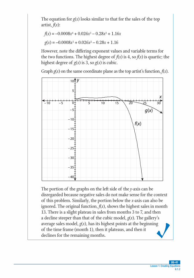
The equation for g(x) looks similar to that for the sales of the top artist, f(x):
f(x) = –0.0008x4 + 0.026x3 – 0.28x2 + 1.16x
g(x) = –0.0008x3 + 0.026x2 – 0.28x + 1.16
However, note the differing exponent values and variable terms for the two functions. The highest degree of f(x) is 4, so f(x) is quartic; the highest degree of g(x) is 3, so g(x) is cubic.
Graph g(x) on the same coordinate plane as the top artist’s function, f(x).
–10 –5 5 10 15 20 25 30
10
5
0
–5
–10
–15
–20
–25
–30
–35
–40
y
x
f(x)
g(x)
The portion of the graphs on the left side of the y-axis can be disregarded because negative sales do not make sense for the context of this problem. Similarly, the portion below the x-axis can also be ignored. The original function, f(x), shows the highest sales in month 13. There is a slight plateau in sales from months 3 to 7, and then a decline steeper than that of the cubic model, g(x). The gallery’s average sales model, g(x), has its highest points at the beginning of the time frame (month 1), then it plateaus, and then it declines for the remaining months.

U6-42
PRACTICE
UNIT 6 • MATHEMATICAL MODELINGLesson 1: Creating Equations
Unit 6: Mathematical Modeling 6.1.2
Use the information that follows to complete problems 1 and 2.
The distance in feet of a hawk swooping down from the sky to grab a mouse on the ground is given by s(t) = 16t2, where t is the time in seconds.
1. Write an equation that represents the time it takes the hawk to reach the mouse if the hawk’s starting height is 576 feet.
2. How long would it take the hawk to reach the mouse from this height?
Use the information that follows to complete problems 3 and 4.
London is a salesperson at a high-end clothing store. She earns $2,000 a month, plus a commission of 20% of the sales she makes. Her goal is to make enough sales to earn $6,000 in one month.
3. Write an equation that represents the amount of sales London needs to make to earn at least $6,000 in one month. Let x represent the amount of sales.
4. Use the equation from problem 3 to determine the amount of sales in dollars London needs to make to earn at least $6,000 in one month.
Practice 6.1.2: Creating Equations in Two Variables
continued
U6-43
PRACTICE
UNIT 6 • MATHEMATICAL MODELINGLesson 1: Creating Equations
Lesson 1: Creating Equations 6.1.2
Use the information that follows to complete problems 5 and 6.
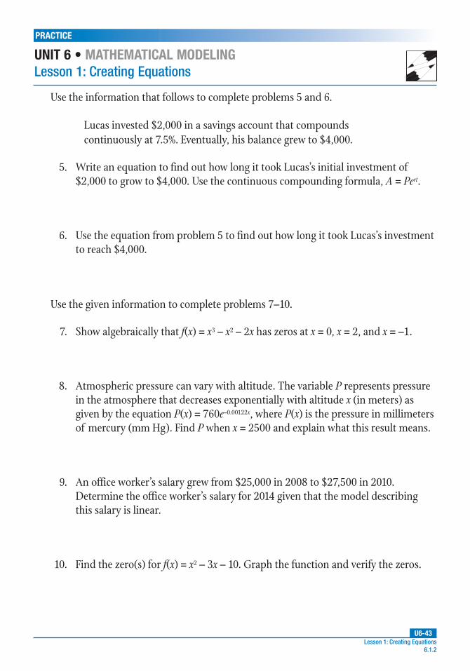
Lucas invested $2,000 in a savings account that compounds continuously at 7.5%. Eventually, his balance grew to $4,000.
5. Write an equation to find out how long it took Lucas’s initial investment of $2,000 to grow to $4,000. Use the continuous compounding formula, A = Pert.
6. Use the equation from problem 5 to find out how long it took Lucas’s investment to reach $4,000.
Use the given information to complete problems 7–10.
7. Show algebraically that f(x) = x3 – x2 – 2x has zeros at x = 0, x = 2, and x = –1.
8. Atmospheric pressure can vary with altitude. The variable P represents pressure in the atmosphere that decreases exponentially with altitude x (in meters) as given by the equation P(x) = 760e–0.00122x, where P(x) is the pressure in millimeters of mercury (mm Hg). Find P when x = 2500 and explain what this result means.
9. An office worker’s salary grew from $25,000 in 2008 to $27,500 in 2010. Determine the office worker’s salary for 2014 given that the model describing this salary is linear.
10. Find the zero(s) for f(x) = x2 – 3x – 10. Graph the function and verify the zeros.
U6-44Unit 6: Mathematical Modeling 6.1.3
Lesson 6.1.3: Creating Exponential and Logarithmic EquationsIntroduction
Exponential functions are ideal for modeling growth and decay phenomena. Equations derived from given information, such as observations, can be used to solve problems that involve forecasting and decision-making based on future events. Equations for modeling growth and decay can also be derived from a general exponential growth model, which is a standard equation that has been proven to work for many cases. In addition to equations, graphs are also helpful because they allow predictions to be made about data.
Key Concepts
• Recall that an exponential function has the general form of f(x) = a(bx) + c.
• An exponential equation with a variable in the exponent can be solved by rewriting it as a logarithm to isolate the variable. For instance, y = bx can be rewritten as x = logb y. The resulting equation is then solved by taking the log, which is an operation that can be computed by hand or on a calculator.
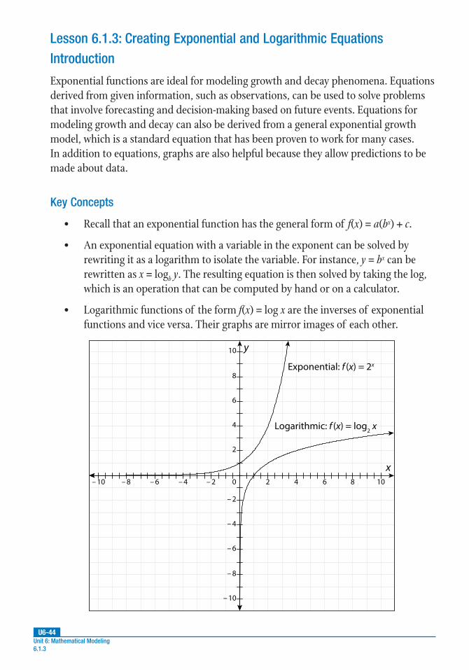
• Logarithmic functions of the form f(x) = log x are the inverses of exponential functions and vice versa. Their graphs are mirror images of each other.
– 10 – 8 – 6 – 4 – 2 2 4 6 8 10
x
10
8
6
4
2
0
– 2
– 4
– 6
– 8
– 10
y
Exponential: f (x) = 2x
Logarithmic: f (x) = log2 x
U6-45Lesson 1: Creating Equations
6.1.3
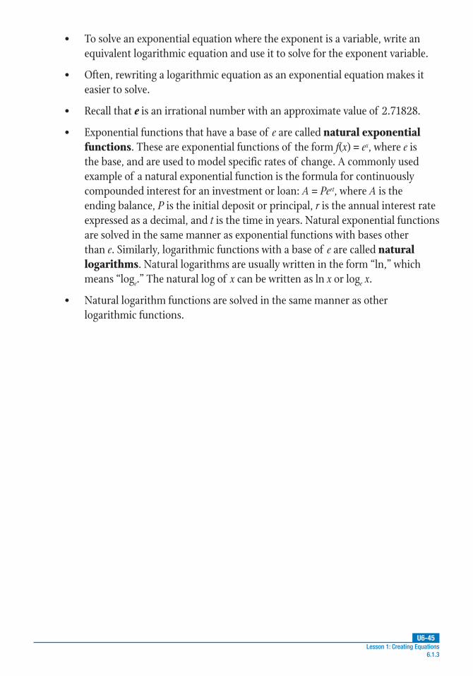
• To solve an exponential equation where the exponent is a variable, write an equivalent logarithmic equation and use it to solve for the exponent variable.
• Often, rewriting a logarithmic equation as an exponential equation makes it easier to solve.
• Recall that e is an irrational number with an approximate value of 2.71828.
• Exponential functions that have a base of e are called natural exponential functions. These are exponential functions of the form f(x) = ex, where e is the base, and are used to model specific rates of change. A commonly used example of a natural exponential function is the formula for continuously compounded interest for an investment or loan: A = Pert, where A is the ending balance, P is the initial deposit or principal, r is the annual interest rate expressed as a decimal, and t is the time in years. Natural exponential functions are solved in the same manner as exponential functions with bases other than e. Similarly, logarithmic functions with a base of e are called natural logarithms. Natural logarithms are usually written in the form “ln,” which means “loge.” The natural log of x can be written as ln x or loge x.
• Natural logarithm functions are solved in the same manner as other logarithmic functions.

U6-46Unit 6: Mathematical Modeling 6.1.3
Guided Practice 6.1.3Example 1
The demand for a particular flat-panel television at a store is given by the exponential function d(x) = 500 – 0.5e0.004x, where d(x) represents the number of TVs sold that week, and x represents the price in dollars. What is the demand level when the TV is priced at $450 versus when it is priced at $400? Which price level will result in higher demand for this TV? Which of the two price levels will yield the most revenue?
1. Determine the demand for the TV at the price level of $450.
Recall that the demand is the number of TVs sold at the given price.
Substitute x = 450 into the original exponential function and solve for d(x).
d(x) = 500 – 0.5e0.004x Original function
d(450) = 500 – 0.5e0.004(450) Substitute 450 for x.
d(450) = 500 – 0.5e1.8 Simplify the exponent.
d(450) ≈ 500 – 0.5(6.05) Evaluate e1.8 using a calculator.
d(450) ≈ 496.98 Simplify.
The demand at the price level of $450 is approximately 496.98.
Since the number of TVs needs to be a whole number, round up so the demand at the price level of $450 is approximately 497 TVs.

U6-47Lesson 1: Creating Equations
6.1.3
2. Determine the demand for the TV at the price level of $400.
Substitute x = 400 into the original exponential function and solve for d(x).
d(x) = 500 – 0.5e0.004x Original function
d(400) = 500 – 0.5e0.004(400) Substitute 400 for x.
d(400) = 500 – 0.5e1.6 Simplify the exponent.
d(400) ≈ 500 – 0.5(4.95) Evaluate e1.6 using a calculator.
d(400) ≈ 497.52 Simplify.
The demand at the price level of $400 is approximately 497.52. Rounded to the nearest whole TV, the demand at $400 is approximately 498 TVs.
3. Determine which price level results in a higher demand.
When comparing the results of steps 1 and 2, we see the demand at the $400 price level is slightly higher (498) than the demand at $450 (497).
4. Which of the two price levels will yield the most revenue?
To determine the revenue for each price level, multiply each price by the number of TVs sold at that price (the demand) and then find the difference.
450 • 497 = 223,650
400 • 498 = 199,200
Though a lower price results in higher demand, the resulting revenue is much lower when the TVs are priced at $400 than when they are priced at $450. The price level of $450 yields higher revenue.

U6-48Unit 6: Mathematical Modeling 6.1.3
Example 2
The percent of males and females between the ages of 18 and 35 who are no more
than x feet tall can be given by the functions =( )1000.6114m x
e x and =( )1000.6661f x
e x , where
m(x) represents the percent of males and f(x) represents the percent of females.
Compare the graphs of the functions. Determine the domain and asymptote for both
graphs, and explain what the domain means in the context of the problem. Then, use
the graphs to draw a conclusion regarding the heights of males and females in this
age range.
1. Graph both functions on the same coordinate plane.
Given that each function has an exponential term of base e in the denominator, using a graphing calculator will be easier than graphing by hand.
The resulting graph of =( )1000.6114m x
e x and =( )1000.6661f x
e x is shown.
Recall that the x-axis represents height in feet and the y-axis represents
the percentage of people at each height.
– 20 – 15 – 10 – 5 5 10 15 20
x
28
26
24
22
20
18
16
14
12
10
8
6
4
2
0– 2
– 4
y
m(x)f(x)

U6-49Lesson 1: Creating Equations
6.1.3
2. Determine the domain of each function and what it means in terms of the context of the problem.
The domain of both graphs is x > 0 because x represents the height in feet of males and females. Height can only be represented by positive numbers, and cannot equal 0. Therefore, the domain is given as the values that are valid heights.
3. Determine the asymptote of each function.
Recall that exponential functions have no vertical asymptotes. It can be seen from the graph that both curves approach y = 0, but do not cross this line. The line y = 0 is a horizontal asymptote. The horizontal asymptote is determined based on the equation. In reality, the curve would approach a line somewhat higher than y = 0 because there are very few individuals in this age range whose height is less than 4 feet.
4. Use the graphs to draw a conclusion regarding the heights of males and females between the ages of 18 and 35.
Both graphs show that the majority of males and females fall between 4 feet and 6 feet in height. The range values on both graphs seem to flatten out or drop drastically once x > 6. The graph representing the percentage of females no more than x feet tall is slightly lower than the graph for males for each domain value, suggesting that females on average are shorter than males.

U6-50Unit 6: Mathematical Modeling 6.1.3
Example 3
The temperature in the freezer compartment of a typical refrigerator is 0°F. The
formula =−−−
5.05 ln40
0 40t
T gives the amount of time (t) in hours that it takes
for the temperature in degrees Fahrenheit (T) of frozen meat to change based on the
surrounding temperature. If a package of frozen meat is moved from the freezer to the
refrigerator compartment to thaw for 7 hours, what will the meat’s temperature be at
the end of those 7 hours? Assuming that the meat has to reach a temperature of 40°F
to be considered thawed enough to cook, is 7 hours enough time to thaw the meat for
cooking? If not, how many total hours would it take to thaw the meat?
1. Determine the temperature of the meat after 7 hours in the refrigerator.
To determine the temperature of the meat after 7 hours, let t = 7. Substitute this value into the provided formula and solve for T, the temperature.
=−−−
5.05 ln40
0 40t
TOriginal formula
=−−−
(7) 5.05 ln40
0 40
TSubstitute 7 for t.
− =−−
1.4 ln40
40
T Simplify the denominator and
divide both sides by –5.05.
=−−
− 40
401.4e
T
Apply the properties of natural logarithms to both sides.
–40e–1.4 = T – 40 Multiply both sides by –40.
–40e–1.4 + 40 = T Add 40 to both sides.
40(1 – e–1.4) = T Factor.
40(1 – 0.25) ≈ T Evaluate e–1.4 using a calculator.
40(0.75) ≈ T Subtract.
30 ≈ T Multiply.
After 7 hours in the refrigerator, the meat will have thawed to approximately 30°F.

U6-51Lesson 1: Creating Equations
6.1.3
2. Determine how many more hours are needed to thaw the meat, if more hours are needed.
After 7 hours, the meat reaches 30°F, but in order to be thawed enough to cook, the meat needs to reach a temperature of 40°F. Therefore, the temperature of the meat needs to increase by 10 degrees.
To determine how many more hours are needed to raise the temperature an additional 10 degrees, first calculate the number of degrees the meat thaws each hour.
=30
7 1
x Create a proportion.
7x = 30 Cross multiply.
x ≈ 4.3 Divide both sides by 7.
The meat’s temperature increased by approximately 4.3°F every hour.
Since the temperature of the meat needs to increase by 10 degrees, divide the remaining 10 degrees by 4.3 to yield the additional hours required to thaw the meat to 40°F.
≈10
4.32.3
Thus, approximately 2.3 more hours must be added on to the original 7 hours.
Therefore, the total amount of time needed to fully thaw the meat would be 7 + 2.3 or approximately 9.3 hours.

U6-52Unit 6: Mathematical Modeling 6.1.3
Example 4
It is predicted that the annual rate of inflation will average about 3% for each of the next 10 years. The estimated cost of goods in any of those years can be written as C(t) = P(1.03)t, where P is the current cost of goods and t is the time in years. If the price of 8 gallons of gas is currently $25, use the function to find the cost of 8 gallons of gas 10 years from now. Graph the original function and use it to verify your calculation.
1. Determine the cost of 8 gallons of gas 10 years from now.
Substitute the known information into the given cost function, C(t) = P(1.03)t, and then solve the resulting equation to determine the price of gas 10 years from now.
Let P (the current cost) equal 25, and let t equal 10.
C(t) = P(1.03)t Original function
C(10) = (25)(1.03)(10) Substitute 25 for P and 10 for t.
C(10) ≈ 33.60 Simplify.
The cost of 8 gallons of gas will be approximately $33.60 in 10 years.
U6-53Lesson 1: Creating Equations
6.1.3
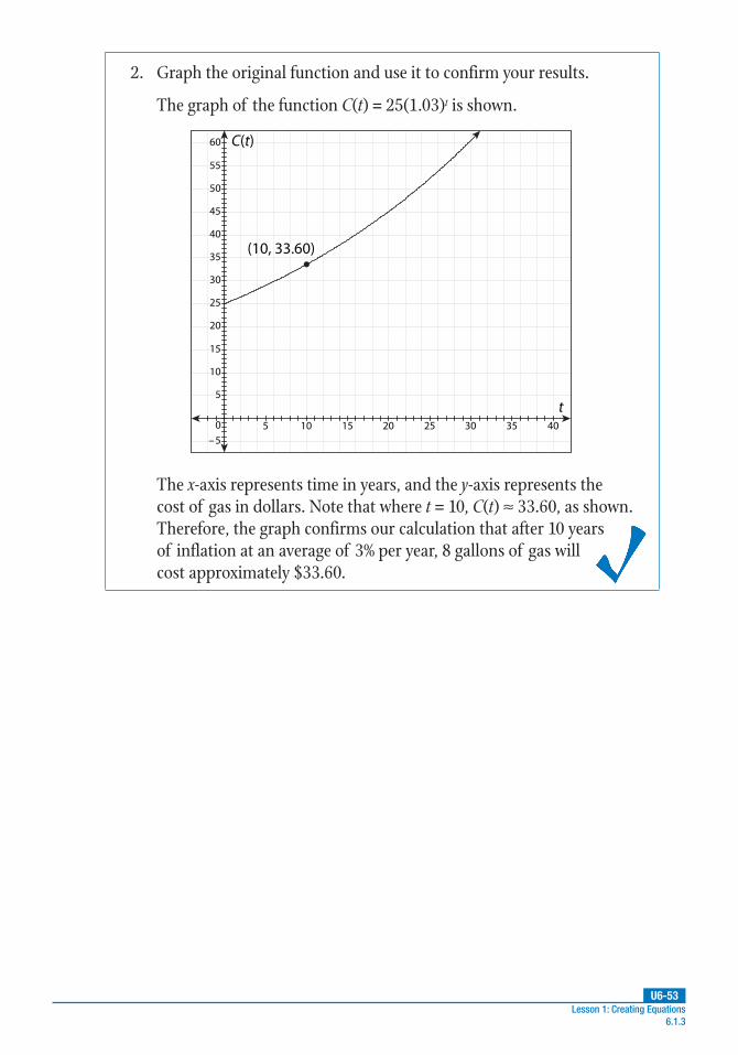
2. Graph the original function and use it to confirm your results.
The graph of the function C(t) = 25(1.03)t is shown.
60
55
50
45
40
35
30
25
20
15
10
5
0
–55 10 15 20 25 30 35 40
C(t)
t
(10, 33.60)
The x-axis represents time in years, and the y-axis represents the cost of gas in dollars. Note that where t = 10, C(t) ≈ 33.60, as shown. Therefore, the graph confirms our calculation that after 10 years of inflation at an average of 3% per year, 8 gallons of gas will cost approximately $33.60.

U6-54
PRACTICE
UNIT 6 • MATHEMATICAL MODELINGLesson 1: Creating Equations
Unit 6: Mathematical Modeling 6.1.3
Use what you know about exponential and logarithmic functions and equations to complete problems 1–6.
1. The function =+ −( )
90
1 271 0.122P xe t models the percentage of adults who are
x years old and show signs of developing heart disease. At what age does the
percentage of adults who show signs of heart disease reach 25%?
2. The squirrel population in a forest grows at a rate of 4% every month. There are 220 squirrels in the forest in August. Use the natural exponential growth equation y = aebt to create a function that could determine how many squirrels, y, would be in the forest after 1 year, where t is the time in years. How many more squirrels will there be after 1 year?
3. If $9,000 is invested at 2.5% compounded annually, what equation would be used to find the balance in the account after 5 years?
4. Use the equation you wrote for problem 3 to find the balance. Round to the nearest hundredth.
5. An isotope of a nuclear material created in a lab is decaying at a rate of 12% each second. If 6 grams of the isotope were created, how many grams remain after 10 seconds? Round your answer to the nearest tenth.
6. Trinity deposited $5,000 into an investment account paying continuously compounded interest at a rate of 6.5%. She checked the balance after 5 years, and again after 10 years. What was the balance of Trinity’s investment each time she checked? Round to the nearest hundredth.
Practice 6.1.3: Creating Exponential and Logarithmic Equations
continued

U6-55
PRACTICE
UNIT 6 • MATHEMATICAL MODELINGLesson 1: Creating Equations
Lesson 1: Creating Equations 6.1.3
Use the information that follows to complete problems 7 and 8.
For the years 1993 to 2012, the average salary y (in thousands) for public school librarians can be modeled by y = –1.562 + 14.584 ln t, where t is the number of years using the range 5 through 24, with t = 5 representing the year 1993.
7. Write an equation to find out when the average salary reached $44,000.
8. Using the equation you wrote for problem 7, what was the year?
Use the information that follows to complete problems 9 and 10.
A city has a population of 48,250 residents and grows by 7.5% each year. The city’s population growth is modeled by the natural exponential equation P = aebt, where a is the starting population, b is the growth rate, and t is the time in years.
9. Use the given equation to write a specific equation to determine how long it will take the city to grow to 114,921 residents.
10. Using the equation you wrote for problem 9, how many years will it take?

U6-56Unit 6: Mathematical Modeling 6.1.4
Lesson 6.1.4: Creating Rational, Radical, and Trigonometric FunctionsIntroduction
Rational functions are ideal for modeling situations that involve relationships between variables that increase or decrease but with some interruption. The graphs of rational functions are helpful in forecasting these “glitches” in data and pinpointing where the continuous patterns of data will stop and start.
Radical equations are most commonly used for scientific and engineering models that involve power, resistance, and speed. Their graphs are curved and also may exhibit areas that are undefined. This kind of information is useful when constructing physical science models because it indicates constraints that must be accommodated.
Additionally, trigonometric functions can be used to model repetitive motions or revolutions of objects, such as a spinning top or a figure skater performing a spin on the ice. The basic trigonometric functions are sine, cosine, and tangent. In this lesson, you will solve problems algebraically and graphically using rational, radical, and trigonometric functions.
Key Concepts
Rational Functions
• Rational functions are functions in the form =( )( )
( )f x
p x
q x, where p(x) and q(x)
are polynomials and q(x) ≠ 0. The numerator, p(x), is a constant or polynomial
function of degree at least 1, and the denominator is a polynomial function
with a degree of at least 1. Examples of rational functions include =+
( )1
1f x
x
and =− −
( )5
22g xx x
.
• Because rational functions consist of fractions, there may be places where the function is undefined. Specifically, when the denominator of the function is 0, the value will be undefined.
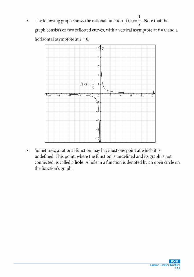
U6-57Lesson 1: Creating Equations
6.1.4
• The following graph shows the rational function =( )1
f xx
. Note that the
graph consists of two reflected curves, with a vertical asymptote at x = 0 and a
horizontal asymptote at y = 0.
–10 –8 –6 –4 –2 2 4 6 8 10
x
10
8
6
4
2
0
–2
–4
–6
–8
–10
y
=f xx
( )1
• Sometimes, a rational function may have just one point at which it is undefined. This point, where the function is undefined and its graph is not connected, is called a hole. A hole in a function is denoted by an open circle on the function’s graph.

U6-58Unit 6: Mathematical Modeling 6.1.4
• For example, the function =− −−
( )2
2
2
f xx x
x is undefined at the point (2, 3), as
shown by the open circle on the graph.
–10 –8 –6 –4 –2 2 4 6 8 10
x
10
8
6
4
2
0
–2
–4
–6
–8
–10
y
• A rational function is undefined at its vertical asymptotes.
• Vertical asymptotes will occur where the denominator is equal to 0 (that is, where the function is undefined).
• If the degree of the numerator is less than the degree of the denominator, then there is a horizontal asymptote at y = 0.
• Also, in a rational function of the form =( )( )
( )f x
p x
q x, if the degree of the
numerator is equal to the degree of the denominator, then there is a horizontal
asymptote at a
b, where a is the leading coefficient of p(x) and b is the leading
coefficient of q(x).
• If the degree of the numerator is greater than the degree of the denominator, then there is no horizontal asymptote.
• The domain of a simple rational function, =( )1
f xx
, is all real numbers except
for x = 0 because =( )1
0f x is undefined.
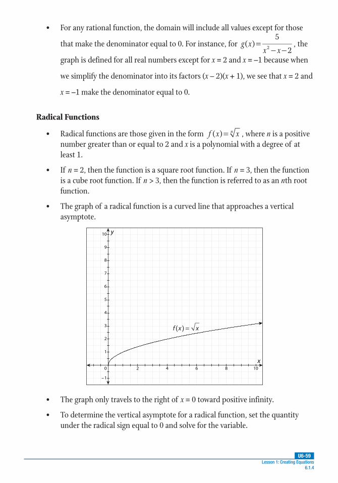
U6-59Lesson 1: Creating Equations
6.1.4
• For any rational function, the domain will include all values except for those
that make the denominator equal to 0. For instance, for =− −
( )5
22g xx x
, the
graph is defined for all real numbers except for x = 2 and x = –1 because when
we simplify the denominator into its factors (x – 2)(x + 1), we see that x = 2 and
x = –1 make the denominator equal to 0.
Radical Functions
• Radical functions are those given in the form =( )f x xn , where n is a positive number greater than or equal to 2 and x is a polynomial with a degree of at least 1.
• If n = 2, then the function is a square root function. If n = 3, then the function is a cube root function. If n > 3, then the function is referred to as an nth root function.
• The graph of a radical function is a curved line that approaches a vertical asymptote.
2 4 6 8 10
x
10
9
8
7
6
5
4
3
2
1
0
–1
y
=f x x( )
• The graph only travels to the right of x = 0 toward positive infinity.
• To determine the vertical asymptote for a radical function, set the quantity under the radical sign equal to 0 and solve for the variable.
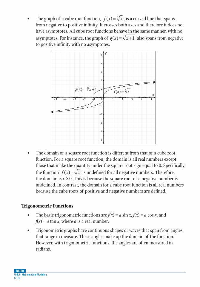
U6-60Unit 6: Mathematical Modeling 6.1.4
• The graph of a cube root function, =( ) 3f x x , is a curved line that spans from negative to positive infinity. It crosses both axes and therefore it does not have asymptotes. All cube root functions behave in the same manner, with no asymptotes. For instance, the graph of = +g x x( ) 13 also spans from negative to positive infinity with no asymptotes.
–5 –4 –3 –2 –1 1 2 3 4 5
x
5
4
3
2
1
0
–1
–2
–3
–4
–5
y
= +g x x( ) 13
=f x x( ) 3
• The domain of a square root function is different from that of a cube root function. For a square root function, the domain is all real numbers except those that make the quantity under the square root sign equal to 0. Specifically, the function =( )f x x is undefined for all negative numbers. Therefore, the domain is x ≥ 0. This is because the square root of a negative number is undefined. In contrast, the domain for a cube root function is all real numbers because the cube roots of positive and negative numbers are defined.
Trigonometric Functions
• The basic trigonometric functions are f(x) = a sin x, f(x) = a cos x, and f(x) = a tan x, where a is a real number.
• Trigonometric graphs have continuous shapes or waves that span from angles that range in measure. These angles make up the domain of the function. However, with trigonometric functions, the angles are often measured in radians.

U6-61Lesson 1: Creating Equations
6.1.4
• The basic sine curve f(x) = sin x is S-shaped and crosses the axis at (0, 0), (0, π), and (0, 2π).
–4 –3 –2 – 2 3 4
x
radians
4
3
2
1
0
–1
–2
–3
–4
y
f(x) = sin x g(x) = cos x
• To convert degrees to radians, multiply the number of degrees by π°180
. For
instance, 90° converted to radians would be π π
°°=90 •
180 2radians.
• The range values for a trigonometric function represent the height or amplitude of the graph.
• In a general sine function of the form f(x) = a sin x, the value of a determines the height of the curve. For instance, the height of the trigonometric curve f(x) = sin x shown in the graph ranges from –1 to 1 on the y-axis. To double the height (amplitude) of the curve, multiply a (understood to be 1) by 2 to yield the equation f(x) = 2 sin x. The height of f(x) = 2 sin x will range from –2 to 2 on the y-axis.
• Trigonometric graphs are endless and technically go on forever. For this reason, when talking about a parent trigonometric function, we define 0 to 2π as a period. The basic curve repeats every period of 2π radians, or 360°. If a graph spans 2 cycles, that means that the graph includes a domain from 0° to 360° twice—that is, it repeats a full cycle twice, from 0 to 2π(2) or 4π. If the graph spans 3 cycles, then the period would be from 0 to 2π(3) or 6π and so on.
• In general, we can write the period of a function as 2πn, where n is the number of times the curve repeats a cycle, 2π. This behavior is known as the periodicity of the function.
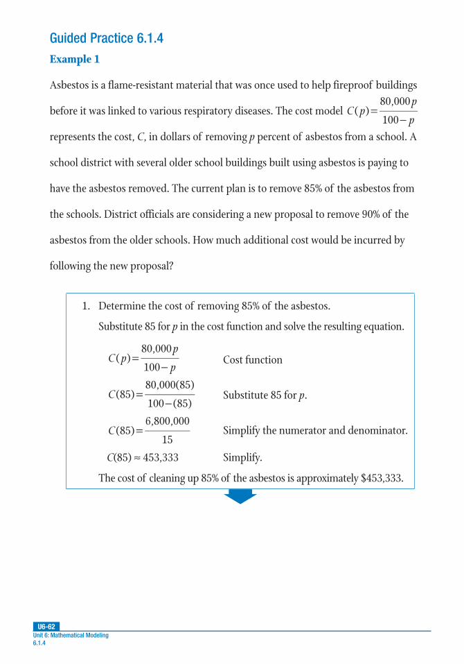
U6-62Unit 6: Mathematical Modeling 6.1.4
Guided Practice 6.1.4Example 1
Asbestos is a flame-resistant material that was once used to help fireproof buildings
before it was linked to various respiratory diseases. The cost model =−
( )80,000
100C p
p
p
represents the cost, C, in dollars of removing p percent of asbestos from a school. A
school district with several older school buildings built using asbestos is paying to
have the asbestos removed. The current plan is to remove 85% of the asbestos from
the schools. District officials are considering a new proposal to remove 90% of the
asbestos from the older schools. How much additional cost would be incurred by
following the new proposal?
1. Determine the cost of removing 85% of the asbestos.
Substitute 85 for p in the cost function and solve the resulting equation.
=−
( )80,000
100C p
p
pCost function
=−
(85)80,000(85)
100 (85)C Substitute 85 for p.
=(85)6,800,000
15C Simplify the numerator and denominator.
C(85) ≈ 453,333 Simplify.
The cost of cleaning up 85% of the asbestos is approximately $453,333.

U6-63Lesson 1: Creating Equations
6.1.4
2. Determine the cost of removing 90% of the asbestos.
Substitute 90 for p in the cost function and solve the resulting equation.
=−
( )80,000
100C p
p
p Cost function
=−
(90)80,000(90)
100 (90)C Substitute 90 for p.
=(90)7,200,000
10C Simplify the numerator and denominator.
C(90) = 720,000 Simplify.
The cost of cleaning up 90% of the asbestos is $720,000.
3. Determine the difference in the costs of the two proposals.
Subtract the results for C(85) and C(90).
720,000 – 453,333 = 266,667
The proposal to remove 90% of the asbestos instead of 85% would cost the school district approximately $266,667 more.
U6-64Unit 6: Mathematical Modeling 6.1.4
Example 2
The human body converts food into glucose (a type of sugar). The glucose enters the
bloodstream, where the hormone insulin helps the cells absorb the glucose to use for
energy. In a healthy person, the amount of insulin in the bloodstream rises and falls
with the amount of glucose present. The amount of insulin left in the bloodstream
after eating a candy bar is represented by the function =−
( )2
1
2
2f xx
x, where f(x) is
the amount of insulin in milligrams per deciliter (mg/dl) in the bloodstream and x
is the elapsed time in minutes since eating the candy bar. Determine the domain of
this function. Then, find the horizontal and vertical asymptotes and interpret their
meaning in the context of this problem. Graph the function to verify your findings.
1. Find the domain of the function.
The domain of a function will be those values of x for which the function is defined. Because f(x) is a rational function, the domain will not include the values that make x2 – 1 = 0 because when the denominator of a fraction is equal to 0, the fraction is undefined. Therefore, the domain of f(x) is x > 1.
In this context, a domain of x > 1 means that we will only consider the amount of insulin remaining after 1 minute has elapsed from the time the candy bar is consumed.

U6-65Lesson 1: Creating Equations
6.1.4
2. Find the horizontal asymptote for the function and interpret it in the context of this problem.
Recall that in a rational function of the form =( )( )
( )f x
p x
q x, if the
degree of p(x) is equal to the degree of q(x), then there is a horizontal
asymptote at a
b, where a is the leading coefficient of p(x) and b is the
leading coefficient of q(x).
For =−
( )2
1
2
2f xx
x, the degree of p(x) = the degree of q(x). Therefore,
to find the horizontal asymptote, divide the leading coefficients of the
numerator and the denominator: 2 and 1. 2 ÷ 1 = 2, so, the horizontal
asymptote is y = 2.
A horizontal asymptote at y = 2 means that as the time in minutes goes on (that is, as x values get larger), the amount of insulin in the bloodstream will keep decreasing as the cells absorb the glucose from the bloodstream. In other words, the insulin level will continue to decrease as time passes, but at a slower rate, and will never drop below 2 mg/dl since the asymptote is located at y = 2.
3. Find and interpret the vertical asymptote.
The vertical asymptotes of a rational function can be found by finding the zeros. Factoring the denominator, x2 – 1, we get (x + 1)(x – 1). Solving each factor for x, we can determine that the function has vertical asymptotes at x = –1 and x = 1.
For this function, the vertical asymptote at x = –1 does not make sense because we cannot measure time as a negative number. Therefore, disregard this asymptote.
A vertical asymptote at x = 1 means that the insulin is not measured until after 1 minute has elapsed. One possible reason for this could be because of the type of insulin test being administered.

U6-66Unit 6: Mathematical Modeling 6.1.4
4. Graph the function and use it to verify your findings.
The graph of =−
( )2
1
2
2f xx
x is shown.
–10 –8 –6 –4 –2 2 4 6 8 10
x
10
8
6
4
2
0
–2
–4
–6
–8
–10
y
From the graph, we can verify the vertical asymptotes at x = –1 and x = 1, and the horizontal asymptote at y = 2. Since the x-axis represents time and the y-axis represents insulin levels, neither of which can be negative, the domain of the function must be in the first quadrant; all other portions of the graph can be ignored. Given the vertical asymptote at x = 1, the domain must be x > 1. Therefore, the graph verifies the previously determined findings.
U6-67Lesson 1: Creating Equations
6.1.4
Example 3
A small airline’s cost per passenger for x number of passengers (in thousands) per year is given by the function = +( ) 0.3 1C x x , where C(x) is measured in millions of dollars and x ≥ 0. Find the airline’s cost for flying 10,000 passengers. If the average ticket price for all classes of tickets is $320 per passenger, find the profit made by the airline for flying 10,000 passengers. How many passengers did the airline have if the total cost was $4 million?
1. Find the profit made by the airline for flying 10,000 passengers.
To compute the cost, let x = 10 because we are given that x is measured in thousands.
= +( ) 0.3 1C x x Original function
= +(10) 0.3(10) 1C Substitute 10 for x.
=(10) 4C Multiply and add.
C(10) = 2 Simplify the expression under the radical.
Since the cost is in millions of dollars, it costs the airline $2 million to fly 10,000 passengers.
2. Calculate the amount of profit given a revenue of $320 per passenger.
To find the profit, first determine the airline’s revenue for 10,000 passengers, then subtract its costs.
At $320 per passenger, the total revenue would be 320 • 10,000 or $3.2 million.
The profit would be $3.2 million – $2 million or $1.2 million.
U6-68Unit 6: Mathematical Modeling 6.1.4
3. Compute the number of passengers required for a total cost of $4 million.
To find the number of passengers, let C(x) = 4, since we’re given that C(x) is measured in millions.
= +( ) 0.3 1C x x Original function
= +(4) 0.3 1x Substitute 4 for C(x).
16 = 0.3x + 1 Square both sides of the equation.
15 = 0.3x Subtract 1 from both sides.
50 = x Divide both sides by 0.3.
Recall that x represents passengers measured in thousands, so x = 50 represents 50 • 1000 = 50,000 passengers.
50,000 passengers would result in a total cost of $4 million.

U6-69Lesson 1: Creating Equations
6.1.4
Example 4
Sketch the graph of f(x) = 2 sin x by hand on the restricted domain from 0 to 4π radians and identify the maxima, minima, and intercepts.
1. Identify the amplitude of the function from its equation, and describe how this value would cause the function’s graph to differ from that of the parent sine function, f(x) = sin x.
The amplitude is the coefficient of the trigonometric term. In this case, it is the number 2 in front of “sin x.” Thus f(x) = 2 sin x is twice the height of the parent sine function, f(x) = sin x, so the maxima will shift up and the minima will shift down by one additional unit.
2. Plot the function.
From the sine graph in the Key Concepts, you know that the basic sine curve f(x) = sin x is S-shaped and crosses the axis at (0, 0), (0, π), and (0, 2π). The curve repeats every period of 2π radians, or 360°. Since f(x) = 2 sin x has an amplitude of 2, its highest and lowest points will be 2 units above and below the x-axis and will occur halfway between the x-intercepts.
Sketch a sine wave following the general shape of the parent function, f(x) = sin x. Remember that the amplitude is now 2 and that the restricted domain is from 0 to 4π.
–4 –3 –2 – 2 3 4
x
radians
4
3
2
1
0
–1
–2
–3
–4
y
f(x) = 2 sin x

U6-70Unit 6: Mathematical Modeling 6.1.4
3. Determine the coordinates of the graph’s intercepts, maxima, and minima for the first two periods of the function.
Refer to the graph to determine the key features.
First period (0 to 2π):
• Intercept: (0, 0)
• Maximum: π
2
,2
• Intercept: (π, 0)
• Minimum: π
−
3
2, 2
• Intercept: (2π, 0)
Second period (2π to 4π):
• Maximum: π
5
2,2
• Intercept: (3π, 0)
• Minimum: π
−
7
2, 2
• Intercept: (4π, 0)

U6-71Lesson 1: Creating Equations
6.1.4
Example 5
The cost, C, of ordering supplies for manufacturing a product can be given by the
function =−
− −( )
9
2 3
2
2C xx
x x, where x is the order size (in hundreds). First, identify all
asymptotes and/or holes in the graph of the function mathematically. Then, use your
findings to graph the function.
1. Factor the original function to make it easier to work with.
Factor the numerator and denominator in the original equation.
=−
− −( )
9
2 3
2
2C xx
x xOriginal function
=+ −− +
( )( 3)( 3)
( 3)( 1)C x
x x
x xFactor the numerator and denominator.
Notice that x cannot equal 3 or –1 because these values would cause the denominator to equal 0 and thus would make the fraction undefined.
2. Find any horizontal asymptotes.
Identify any horizontal asymptotes by using the factored function from the previous step.
Recall that in a rational function of the form =( )( )
( )f x
p x
q x, if the
degree of p(x) is equal to the degree of q(x), then there is a horizontal
asymptote at a
b, where a is the leading coefficient of p(x) and b is the
leading coefficient of q(x).
Since the degree of the numerator is equal to the degree of the denominator in the equation for C(x), divide the leading coefficients of the numerator and denominator: 1 and 1. Therefore, there is a horizontal asymptote at 1 ÷ 1 or y = 1.

U6-72Unit 6: Mathematical Modeling 6.1.4
3. Find any vertical asymptotes and/or holes in the function’s graph.
Identify any vertical asymptotes and/or holes by finding the zeros.
To find the zeros, solve for x in the denominator of the factored function. From (x – 3)(x + 1), we can determine that the zeros are located at x = 3 and x = –1. Simplify the factored function, and then substitute each zero into it to determine any holes or asymptotes.
=+ −− +
( )( 3)( 3)
( 3)( 1)C x
x x
x xFactored function
=++
( )( 3)
( 1)C x
x
xDivide both the numerator and denominator by (x – 3).
=++
=( )(3) 3
(3) 11.5C x Substitute x = 3 and solve.
For the first zero, when x = 3, C(x) = 1.5, so a hole exists at (3, 1.5).
Next, substitute x = –1 into the simplified function and solve.
=− +− +
=( )( 1) 3
( 1) 1undefinedC x
For the second zero, when x = –1, C(x) is undefined, so there is a vertical asymptote at x = –1.

U6-73Lesson 1: Creating Equations
6.1.4
4. Sketch the graph of =−
− −( )
9
2 3
2
2C xx
x x by hand.
Use the zero points and the asymptotes found in previous steps. The vertical asymptote is at x = –1, the horizontal asymptote is at y = 1, and the hole is at (3, 1.5).
Use two to three additional points to create the graph. When finding the extra points, substitute x-values into the original function, not the simplified function. Also, make sure that you choose x-values that adhere to the asymptotes and hole. In other words, avoid using x = 3 and x = –1.
–20 –15 –10 –5 5 10 15 20 x
20
18
16
14
12
10
8
6
4
2
0–2
–4
–6
–8
–10
–12
–14
–16
–18
–20
y
=−
− −C x
x
x x( )
9
2 3
2
2
There is a horizontal asymptote at y = 1 and a vertical asymptote
at x = –1. A hole in the graph exists at the point (3, 1.5).
U6-74
PRACTICE
UNIT 6 • MATHEMATICAL MODELINGLesson 1: Creating Equations
Unit 6: Mathematical Modeling 6.1.4
Use the information that follows to complete problems 1–3.
The concentration, C , of a medication found in the bloodstream
x hours after an injection is given by =+ −5
62Cx
x x.
1. Find any horizontal asymptotes and interpret their meaning in the context of this problem.
2. Find any vertical asymptotes and interpret their meaning in the context of this problem.
3. Identify any holes in the graph of the function and indicate what they mean in the context of this problem.
Use the information that follows to complete problems 4–6.
The owner of a luggage shop created a forecast to predict his future
monthly sales using the function π
= +( ) 74.5 44 cos6
L xx
, where L(x)
represents the sales in thousands of dollars and x is the number of
months over a 15-month period, with x = 0 representing the first
January of the months covered by the forecast.
4. Graph the function.
5. Use the graph to determine which months will have the most sales. What are those months and what are the predicted sales for each individual month?
6. Use the graph to determine which month(s) will have the least sales, and the amount of predicted sales for each month.
Practice 6.1.4: Creating Rational, Radical, and Trigonometric Functions
continued

U6-75
PRACTICE
UNIT 6 • MATHEMATICAL MODELINGLesson 1: Creating Equations
Lesson 1: Creating Equations 6.1.4
Use the information that follows to complete problems 7 and 8.
A store’s profits from selling a certain model of children’s bicycles can be modeled with the function P(x) = 360x – 56,000, where x is the number of bicycles sold.
7. What is the average profit function?
8. What is the average profit per bike from selling 224 bicycles?
Use the given information to complete problems 9 and 10.
9. Use periodicity to find π
π+
sin2
2 .
10. Compare the amplitudes for the graphs of f(x) = 2 sin x and g(x) = sin (x – π).
Lesson 2: Piecewise, Step, and Absolute Value Functions
UNIT 6 • MATHEMATICAL MODELING
U6-76Unit 6: Mathematical Modeling 6.2
Common Core Georgia Performance Standards
MCC9–12.A.CED.2★
MCC9–12.F.IF.4★
MCC9–12.F.IF.5★
MCC9–12.F.IF.7b★
Essential Questions
1. What is the difference between a piecewise function and a step function?
2. What does a solid circle on the graph of a step function indicate? What does an open circle indicate?
3. What happens to the domain of a piecewise function or step function if the inequality symbol in the interval for domain values changes from < or > to ≤ or ≥?
4. What is the standard form of an absolute value function and what does it mean in terms of the graph of the function?
5. Given the graphs of f x x c( )= + and f x x c( )= + , where c is a constant, how do the vertices and shapes of the graphs differ?
WORDS TO KNOW
absolute value function a function of the form f x a x h k( )= − + , where x is the independent variable, and a, h, and k are real numbers.
ceiling function a function represented as y x= . For any input x, the output is the smallest integer greater than or equal to x; also called the least integer function
continuous function a function that does not have a break in its graph across a specified domain
discontinuous function a function that has a break, hole, or jump in the graph
floor function a function represented as y x= . For any input x, the output is the largest integer less than or equal to x; also called the greatest integer function

U6-77Lesson 2: Piecewise, Step, and Absolute Value Functions
6.2
greatest integer function a function represented as y x= . For any input x, the output is the largest integer less than or equal to x; also called the floor function
interval a set of values between a lower bound and an upper bound
least integer function a function represented as y x= . For any input x, the output is the smallest integer greater than or equal to x; also called the ceiling function
piecewise function a function that is defined by two or more expressions on separate portions of the domain
stair function a function that is a series of disconnected constant functions; also known as a step function
step function a function that is a series of disconnected constant functions; also known as a stair function
Recommended Resources
• Algebra-Class.com. “Step Functions.”
http://www.walch.com/rr/00246
This site gives a thorough review of the parts of step functions and how to read them.
• Khan Academy. “Finding a piecewise function definition from a graph.”
http://www.walch.com/rr/00267
This video tutorial covers how to find the equations for the steps of a piecewise function by examining the intervals over which the graph of a function is defined.

U6-78Unit 6: Mathematical Modeling 6.2
• OnlineMathLearning.com. “Piecewise Functions.”
http://www.walch.com/rr/00268
This site contains a collection of five videos that demonstrate graphing piecewise functions. The first three videos graph three different piecewise functions. The fourth video covers finding the domain and range of a piecewise function. The fifth video shows the steps involved in writing a function given a piecewise graph.
• Purplemath.com. “Graphing Absolute-Value Functions.”
http://www.walch.com/rr/00269
This site reviews how to use a table of values to graph an absolute value function.
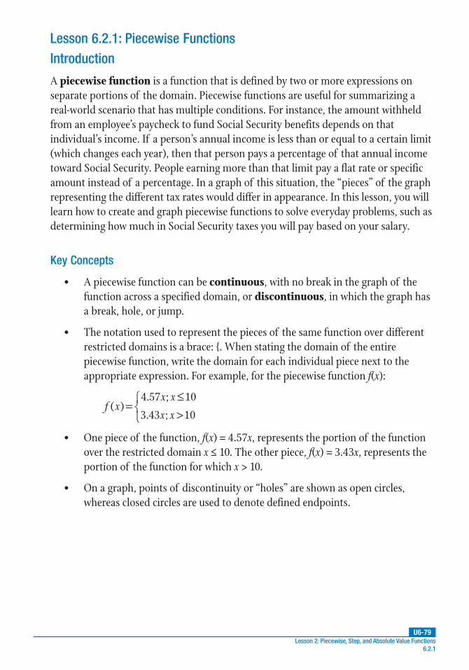
U6-79Lesson 2: Piecewise, Step, and Absolute Value Functions
6.2.1
Introduction
A piecewise function is a function that is defined by two or more expressions on separate portions of the domain. Piecewise functions are useful for summarizing a real-world scenario that has multiple conditions. For instance, the amount withheld from an employee’s paycheck to fund Social Security benefits depends on that individual’s income. If a person’s annual income is less than or equal to a certain limit (which changes each year), then that person pays a percentage of that annual income toward Social Security. People earning more than that limit pay a flat rate or specific amount instead of a percentage. In a graph of this situation, the “pieces” of the graph representing the different tax rates would differ in appearance. In this lesson, you will learn how to create and graph piecewise functions to solve everyday problems, such as determining how much in Social Security taxes you will pay based on your salary.
Key Concepts
• A piecewise function can be continuous, with no break in the graph of the function across a specified domain, or discontinuous, in which the graph has a break, hole, or jump.
• The notation used to represent the pieces of the same function over different restricted domains is a brace: {. When stating the domain of the entire piecewise function, write the domain for each individual piece next to the appropriate expression. For example, for the piecewise function f(x):
f xx x
x x( )
4.57 ; 10
3.43 ; 10=
≤>
• One piece of the function, f(x) = 4.57x, represents the portion of the function over the restricted domain x ≤ 10. The other piece, f(x) = 3.43x, represents the portion of the function for which x > 10.
• On a graph, points of discontinuity or “holes” are shown as open circles, whereas closed circles are used to denote defined endpoints.
Lesson 6.2.1: Piecewise Functions
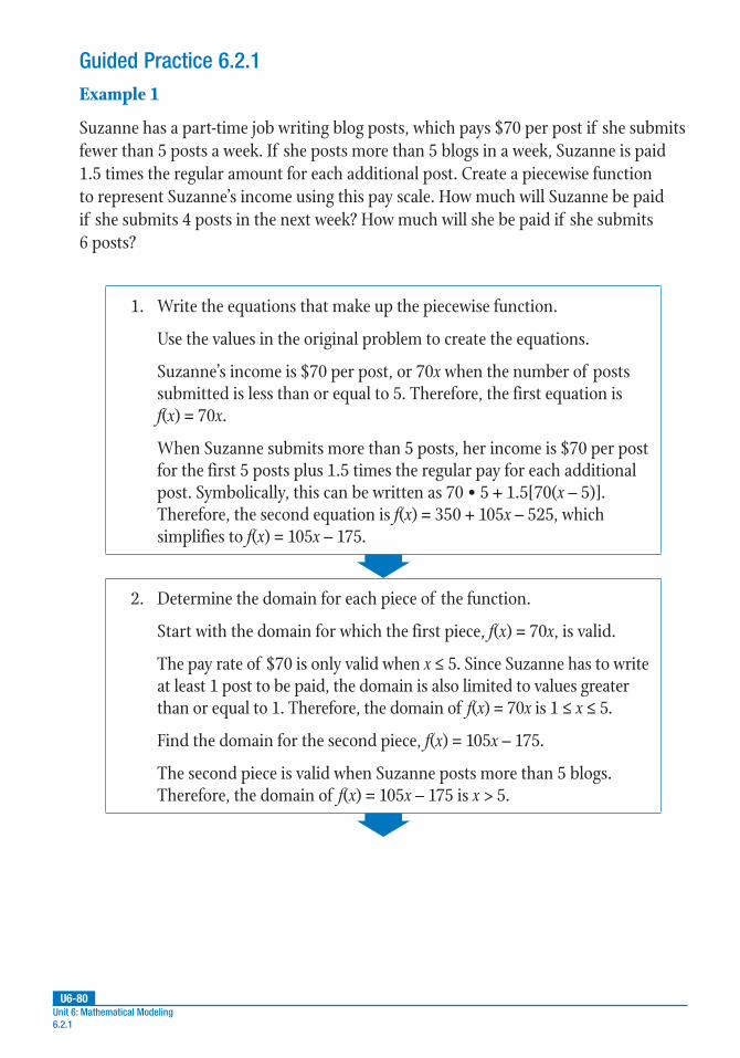
U6-80Unit 6: Mathematical Modeling 6.2.1
Guided Practice 6.2.1Example 1
Suzanne has a part-time job writing blog posts, which pays $70 per post if she submits fewer than 5 posts a week. If she posts more than 5 blogs in a week, Suzanne is paid 1.5 times the regular amount for each additional post. Create a piecewise function to represent Suzanne’s income using this pay scale. How much will Suzanne be paid if she submits 4 posts in the next week? How much will she be paid if she submits 6 posts?
1. Write the equations that make up the piecewise function.
Use the values in the original problem to create the equations.
Suzanne’s income is $70 per post, or 70x when the number of posts submitted is less than or equal to 5. Therefore, the first equation is f(x) = 70x.
When Suzanne submits more than 5 posts, her income is $70 per post for the first 5 posts plus 1.5 times the regular pay for each additional post. Symbolically, this can be written as 70 • 5 + 1.5[70(x – 5)]. Therefore, the second equation is f(x) = 350 + 105x – 525, which simplifies to f(x) = 105x – 175.
2. Determine the domain for each piece of the function.
Start with the domain for which the first piece, f(x) = 70x, is valid.
The pay rate of $70 is only valid when x ≤ 5. Since Suzanne has to write at least 1 post to be paid, the domain is also limited to values greater than or equal to 1. Therefore, the domain of f(x) = 70x is 1 ≤ x ≤ 5.
Find the domain for the second piece, f(x) = 105x – 175.
The second piece is valid when Suzanne posts more than 5 blogs. Therefore, the domain of f(x) = 105x – 175 is x > 5.

U6-81Lesson 2: Piecewise, Step, and Absolute Value Functions
6.2.1
3. Combine the results of steps 1 and 2 to write the piecewise function.
When writing a piecewise function, write the equation of each piece to the right of a brace, with its domain next to it. Each piece and domain is grouped on a separate line.
The piecewise function that represents Suzanne’s weekly income is
( )70 ; 1 5
105 175; 5=
≤ ≤− < <∞
f xx x
x x.
Note that x is not less than 1, since she cannot submit less than a whole post, nor can she submit a negative post. Therefore, in either piece of the function, x is greater than or equal to 1.
4. Use the piecewise function to calculate Suzanne’s income for 4 posts in one week.
If 4 posts are submitted, Suzanne’s income is based on the first equation of the piecewise function, f(x) = 70x, because 4 ≤ 5. Substitute 4 for x in the first piece of the function and then solve.
f(x) = 70x First piece of the function
f(4) = 70(4) Substitute 4 for x.
f(4) = 280 Simplify.
Suzanne’s income for submitting 4 posts in one week is $280.
5. Use the piecewise function to calculate Suzanne’s income for 6 posts.
For 6 posts, Suzanne’s income is based on the second equation of the piecewise function, f(x) = 105x – 175, because 6 > 5. Substitute 6 for x in the second piece of the function and then solve.
f(x) = 105x – 175 Second piece of the function
f(6) = 105(6) – 175 Substitute 6 for x.
f(6) = 630 – 175 Simplify.
f(6) = 455 Subtract.
Suzanne’s income for submitting 6 posts in one week is $455.
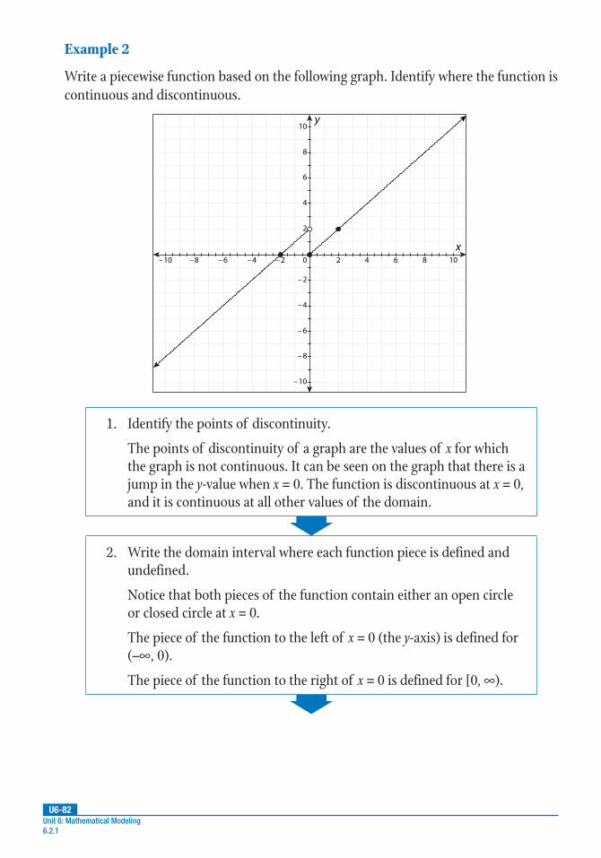
U6-82Unit 6: Mathematical Modeling 6.2.1
Example 2
Write a piecewise function based on the following graph. Identify where the function is continuous and discontinuous.
–10 –8 –6 –4 –2 20 4 6 8 10
x
10
8
6
4
2
–2
–4
–6
–8
–10
y
1. Identify the points of discontinuity.
The points of discontinuity of a graph are the values of x for which the graph is not continuous. It can be seen on the graph that there is a jump in the y-value when x = 0. The function is discontinuous at x = 0, and it is continuous at all other values of the domain.
2. Write the domain interval where each function piece is defined and undefined.
Notice that both pieces of the function contain either an open circle or closed circle at x = 0.
The piece of the function to the left of x = 0 (the y-axis) is defined for (–∞, 0).
The piece of the function to the right of x = 0 is defined for [0, ∞).

U6-83Lesson 2: Piecewise, Step, and Absolute Value Functions
6.2.1
3. Rewrite the domain intervals as inequalities in terms of x.
(–∞, 0) can be rewritten as –∞ < x < 0.
[0, ∞) can be rewritten as 0 ≤ x < ∞.
4. Determine the equations for each piece of the graph.
The piecewise function is comprised of two straight lines; therefore, each piece will be a linear function of the form f(x) = mx + b, where m is the slope and b is the y-intercept.
The piece of the function to the left of x = 0 contains the points (0, 2) and (–1, 1).
Use these points to find the slope of the line. Recall that the slope
formula is my y
x x2 1
2 1
=−−
. Let (x1, y1) be (0, 2) and (x2, y2) be (–1, 1).
Substitute these values into the slope formula and solve for m.
my y
x x2 1
2 1
=−− Slope formula
m(1) (2)
( 1) (0)=
−− −
Substitute 0 for x1, 2 for y1, –1 for x2, and 1 for y2.
m1
1=−−
Simplify.
m = 1 Divide.
It can be observed from the graph that the line crosses the y-axis at the point (0, 2). Therefore, the value of b (the y-intercept) is 2.
The equation of the line to the left of x = 0 in the form f(x) = mx + b is f(x) = 1x + 2, which simplifies to f(x) = x + 2.
Follow the same method to find the equation for the piece of the function to the right of x = 0.
(continued)

U6-84Unit 6: Mathematical Modeling 6.2.1
To find m, substitute the points (0, 0) and (2, 2) shown on the graph
into the slope formula, my y
x x2 1
2 1
=−−
, and solve. Let (x1, y1) be (0, 0)
and (x2, y2) be (2, 2).
my y
x x2 1
2 1
=−− Slope formula
m(2) (0)
(2) (0)=
−−
Substitute 0 for x1, 0 for y1, 2 for x2, and 2 for y2.
m2
2= Simplify.
m = 1 Divide.
It can be observed from the graph that the line crosses the y-axis at the point (0, 0). Therefore, the value of b is 0.
The equation of the line to the right of x = 0 in the form f(x) = mx + b is f(x) = 1x + 0, which simplifies to f(x) = x.
5. Use the results of the previous steps to write the final piecewise function. Indicate the domain intervals for each piece.
The function f(x) = x + 2 is defined for (–∞, 0) or –∞ < x < 0, which can be written as x < 0. The function f(x) = x is defined for [0, ∞) or 0 ≤ x < ∞, which can be written as x ≥ 0.
The piecewise function can be written as ( )2; 0
; 0=
+ <≥
f xx x
x x.

U6-85Lesson 2: Piecewise, Step, and Absolute Value Functions
6.2.1
Example 3
Use the following graph to identify the domain of the function and where the graph is continuous and discontinuous.
1 2 3 4 5 6 7 8 9 10
x
30
28
26
24
22
20
18
16
14
12
10
8
6
4
2
0
y
1. Identify the domain of the piecewise function.
The domain of the function is the x-values for which the function exists.
It can be seen from the graph that the function exists on the intervals (0, 1] and (2, ∞).
2. Use the graph to identify where the function is continuous and discontinuous.
The function is continuous on intervals where the graph is a single unbroken curve. Therefore, the function is continuous on the intervals (0, 1], (2, 5], and (5, ∞).
The function is discontinuous at the x-values that are represented by a break or a jump in the graph. Therefore, this function is discontinuous on the intervals (–∞, 0), (1, 2], and at the point x = 5.

U6-86
PRACTICE
UNIT 6 • MATHEMATICAL MODELINGLesson 2: Piecewise, Step, and Absolute Value Functions
Unit 6: Mathematical Modeling 6.2.1
For problems 1 and 2, evaluate each piecewise function for the given value of x.
1. Evaluate f xx x
xx
( )
13.2 ; 8
2
5; 8
=<
≥
for x = 8.
2. Evaluate f xx x
x x( )
4 8; 5 12
2 6; 5
2
=+ − < ≤− >−
for x = –5.
For problems 3–5, use the description of each piecewise function to solve the problems.
3. A website that helps musicians sell their albums digitally charges transaction fees based on the number of copies sold of each album. The transaction fee is 4% when fewer than 500 albums are sold, 3% for between 500 and 1,000 albums, and 2% for 1,000 or more albums sold. If a musician charges $5 for a particular album, prior to paying any transaction fees, how much would he make on 800 albums sold? What transaction fee percentage would he be charged? How much would he pay in transaction fees?
4. A particular state charges income tax of 6.5% on the first $30,000 of an individual’s annual income, and 8% for any amount greater than $30,000. Mike makes $16,000 a year and Kevin makes $36,000. How much will each man pay in state income taxes? What piecewise function did you use to find this answer?
5. Petra is a diabetic who injects herself with insulin each morning. The following function represents the level of insulin, I(t), in her bloodstream t hours after injection:
I t
t t
t
t t
t
( )
40 100; 0 3
220; 3 8
80 860; 8 10
60; 10 24
=
+ ≤ ≤< ≤
− + < ≤< ≤
If Petra takes her insulin at 6 a.m., find the units of insulin in her bloodstream at 7 a.m., 9 a.m., and 5 p.m.
Practice 6.2.1: Piecewise Functions
continued

U6-87
PRACTICE
UNIT 6 • MATHEMATICAL MODELINGLesson 2: Piecewise, Step, and Absolute Value Functions
Lesson 2: Piecewise, Step, and Absolute Value Functions 6.2.1
For problems 6–10, create a piecewise graph of each scenario and use it to solve the problem.
6. Anson pays a small-business tax at a rate of 15% for the first $20,000 of his company’s income, and pays twice the square root of the income for all income greater than $20,000. Write and graph the function for this scenario. What is the total amount of tax that Anson will pay if his company’s income is $25,000?
7. Sienna rented a car for 6 days for a road trip. The car rental company charges $50 per day plus $0.25 per mile up to and including 100 miles per day. The mileage cost drops to $0.10 per mile for any number of miles greater than 100 per day. What piecewise function determines the total charged for the rental of the car based on the mileage, m? Graph this function and determine the total cost of renting the car if Sienna drove 2,500 miles over the course of her trip.
8. A pet groomer charges $35 per visit for dogs that weigh up to 15 pounds and $40 per visit for dogs that weigh between 15 and 40 pounds. If a dog weighs more than 40 pounds, the charge is $40 plus $2 per pound for the number of pounds greater than 40. Graph the function to determine the charge for a 60-pound dog.
Use what you have learned about piecewise functions to complete problems 9 and 10.
9. Which expression of the piecewise function f xx x
x x( )
2 8; 2
; 22=
+ ≤−
>−
increases over
the interval (–∞, –2)?
10. How many points of discontinuity does the function f x
x x
x
x x
( )
4; 1
2; 1 4
5 ; 4
=+ <≤ ≤
− + ≥
have?

U6-88Unit 6: Mathematical Modeling 6.2.2
Lesson 6.2.2: Step FunctionsIntroduction
A step function is a function that is a series of disconnected constant functions. This type of function is also referred to as a stair function because when graphed, the function resembles a staircase. Step functions are similar to piecewise functions in that these functions consist of several expressions over intervals combined into one function. A step function is useful when there are many cases for small continuous intervals of the domain.
Key Concepts
• A step function is a combination of one or more functions that are defined over restricted intervals, and which may be undefined at other domain points or over other restricted domain intervals.
• A common type of step function is one in which the function values are restricted to integer domain values, such as the number of students who join the computer-gaming club; each student must be represented by a whole number (integer) value.
• By contrast, a function that models temperature changes throughout the day would not be restricted to integer domain values, since temperatures can fluctuate by fractions of degrees.
• Two special types of step functions are called the floor function and the ceiling function.
Floor Functions
• The floor function, sometimes known as the greatest integer function, can be written symbolically as x .
• Floor functions are functions where for any input x, the output is the largest integer less than or equal to x. For example, 2.4 is equal to 2 because 2 is the greatest integer that is less than or equal to 2.4.

U6-89Lesson 2: Piecewise, Step, and Absolute Value Functions
6.2.2
• The following graph displays a floor function, y x = .
–5 –4 –3 –2 –1 0 1 2 3 4 5
–5
–4
–3
–2
–1
1
2
3
4
5 y
x
• Notice the domain (x-values) is all real numbers but the range (y-values) is restricted to integers.
• The floor function is not a continuous function. The open circles indicate where the function is not defined and the closed circles indicate where the function is defined.
• The function increases as the x-values approach positive infinity.
• Adding a constant to a floor function causes its graph to shift up or down depending on the sign of the function. For instance, for f x x c( ) = + , adding c would shift the steps in the graph up by c units, while the steps in the graph of f x x c( ) – = would be shifted down by c units.
Ceiling Functions
• The ceiling function, sometimes known as the least integer function, can be written symbolically as x .
• Ceiling functions are where for any input x, the output is the smallest integer greater than or equal to x. For example, 3.5 is equal to 4 because 4 is the least integer that is greater than or equal to 3.5.
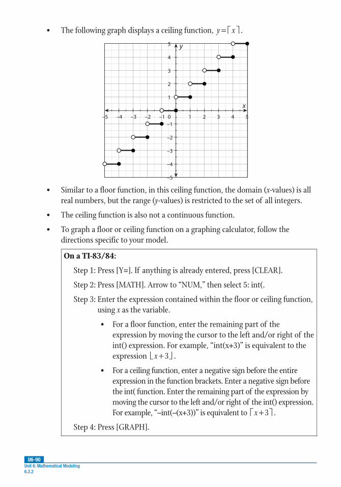
U6-90Unit 6: Mathematical Modeling 6.2.2
• The following graph displays a ceiling function, y x = .
–5 –4 –3 –2 –1 0 1 2 3 4 5
–5
–4
–3
–2
–1
1
2
3
4
5 y
x
• Similar to a floor function, in this ceiling function, the domain (x-values) is all real numbers, but the range (y-values) is restricted to the set of all integers.
• The ceiling function is also not a continuous function.
• To graph a floor or ceiling function on a graphing calculator, follow the directions specific to your model.
On a TI-83/84:
Step 1: Press [Y=]. If anything is already entered, press [CLEAR].
Step 2: Press [MATH]. Arrow to “NUM,” then select 5: int(.
Step 3: Enter the expression contained within the floor or ceiling function, using x as the variable.
• For a floor function, enter the remaining part of the expression by moving the cursor to the left and/or right of the int() expression. For example, “int(x+3)” is equivalent to the expression x 3 + .
• For a ceiling function, enter a negative sign before the entire expression in the function brackets. Enter a negative sign before the int( function. Enter the remaining part of the expression by moving the cursor to the left and/or right of the int() expression. For example, “–int(–(x+3))” is equivalent to x 3 + .
Step 4: Press [GRAPH].

U6-91Lesson 2: Piecewise, Step, and Absolute Value Functions
6.2.2
On a TI-Nspire:
Step 1: Press the [home] key.
Step 2: Arrow over to the graphing icon and press [enter].
Step 3: Enter the expression at the bottom of the application, using x as the variable. Press the catalog key (to the right of the number 9).
• Select floor() to enter a greatest integer expression; for example, typing “floor(x+3)” is equivalent to the expression
x 3 + .
• Select ceiling() to enter a least integer expression; for example, typing “ceiling(x+3)” is equivalent to the expression x 3 + .
Step 4: Press [enter] to plot the expression on the graph.

U6-92Unit 6: Mathematical Modeling 6.2.2
Guided Practice 6.2.2Example 1
Consider the least integer (ceiling) function g x x( )= . How does the value of g(x) change as x changes from 1.5 to 3.8? Graph the function to show the change.
1. Evaluate g(x) at x = 1.5.
A least integer function finds the smallest integer greater than or equal to the given value of x. So, when the function g(x) is evaluated at x = 1.5, the result is g x( ) 1.5 2= = .
2. Evaluate g(x) at x = 3.8.
The smallest integer greater than or equal to 3.8 is 4; therefore, g x( ) 3.8 4= = .
3. Determine how the value of g(x) changes as x changes from 1.5 to 3.8.
When the function g(x) is evaluated at x = 1.5, the result is 2; for x = 3.8, the result is 4. This is a difference of 4 – 2, or 2.
The value of g(x) increases by 2 as x changes from 1.5 to 3.8.

U6-93Lesson 2: Piecewise, Step, and Absolute Value Functions
6.2.2
4. Graph the function g(x) to show this change.
The function g x x( )= can be graphed by hand or using a calculator. The result of either method will resemble the following graph. Notice that each expression is a horizontal line. Endpoints that are not included in the individual domain intervals are represented by an open circle. Endpoints that are included in individual domain intervals are represented by a closed circle.
–2 –1 1 2 3 4 5 6
x
8
7
6
5
4
3
2
1
0
–1
y
(3.8, 4)
(1.5, 2)
Notice the increase of 2 units along the y-axis when x = 1.5 compared to when x = 3.8. This confirms the change in g(x) noted in step 3.

U6-94Unit 6: Mathematical Modeling 6.2.2
Example 2
Consider the function f x x( ) 3= . Graph f(x) and identify the domain and any points of discontinuity for this function.
1. Graph the function by hand or using a graphing calculator.
The graph of f x x( ) 3= is shown. Notice that each expression is a horizontal line. Endpoints that are not included in the individual domain intervals are represented by open circles. Included endpoints in domain intervals are represented by closed circles.
–5 5 10 15
x
15
14
13
12
11
10
9
8
7
6
5
4
3
2
1
0–1
–2
y
2. Identify the domain of f(x).
Notice from the graph that the domain (set of all x-values) is all real numbers.

U6-95Lesson 2: Piecewise, Step, and Absolute Value Functions
6.2.2
3. Identify any points of discontinuity for f(x).
The function is discontinuous for all integer values of x with points of discontinuity on the left end of each line segment when x = …, –2, –1, 0, 1, 2, 3, 4, 5, and so on. Some of the points of discontinuity are (0, 3), (1, 6), and (2, 9); however, if the graph’s axes were extended to show more values, there would be several more. Notice that the y-values increase by 3 each time, and 3 is the coefficient in the original equation f x x( ) 3= .

U6-96Unit 6: Mathematical Modeling 6.2.2
Example 3
Write the equation of the step function shown in the following graph.
–5 –4 –3 –2 –1 1
x
7
6
5
4
3
2
1
0
–1
–2
y
1. Determine the equations for each of the steps of the function.
Begin by looking at the equations of the steps in each interval. It can be seen that there are 5 horizontal steps: f(x) = 1, f(x) = 2, f(x) = 3, f(x) = 4, and f(x) = 5.
Begin writing the function using these equations and the appropriate inequality symbols for the endpoints shown.
f x
x
x
x
x
x
( )
1; ? ?
2; ? ?
3; ? ?
4; ? ?
5; ? ?
=
< ≤< ≤< ≤< ≤< ≤

U6-97Lesson 2: Piecewise, Step, and Absolute Value Functions
6.2.2
2. Identify the intervals for which each step is defined.
Refer to the endpoints of each graphed step. An open circle indicates that the function is undefined at this point and the x-value of the point is not included in the function. A closed circle indicates that the function is defined at this point and the x-value is included in the function.
• The step at f(x) = 1 has an open circle at (–1, 1) and a closed circle at (0, 1). The open circle shows that the function is undefined at (–1, 1) and the value x = –1 is not included in the function. The closed circle means that the function is defined at (0, 1), so x = 0 is included. The step f(x) = 1 is only defined between the values of x = –1 and x = 0, not including –1 but including 0. Therefore, the interval for f(x) = 1 is –1 < x ≤ 0.
• f(x) = 2 has an open circle at (–2, 2) and a closed circle at (–1, 2). The function is undefined at (–2, 2), so x = –2 is not included. The function is defined at (–1, 2), so x = –1 is included. Since f(x) = 2 is only defined between the values of x = –2 and x = –1, not including –2 but including –1, its interval is –2 < x ≤ –1.
• f(x) = 3 is undefined at (–3, 3), so x = –3 is not included. The function is defined at (–2, 3), so x = –2 is included. Since f(x) = 3 is only defined between the values of x = –3 and x = –2, not including –3 but including –2, its interval is –3 < x ≤ –2.
• f(x) = 4 is undefined at (–4, 4) and defined at (–3, 4), so x = –4 is not included but x = –3 is included. Since f(x) = 4 is only defined between the values of x = –4 and x = –3, not including –4 but including –3, its interval is –4 < x ≤ –3.
• f(x) = 5 is undefined at (–5, 5) and defined at (–4, 5), so x = –5 is not included but x = –4 is included. Therefore, its interval is –5 < x ≤ –4.

U6-98Unit 6: Mathematical Modeling 6.2.2
3. Use these intervals to complete the step function of the graph.
Insert each given interval to the right of the equation of its line.
The function f x
x
x
x
x
x
( )
1; 1 0
2; 2 1
3; 3 2
4; 4 3
5; 5 4
=
− < ≤− < ≤−− < ≤−− < ≤−− < ≤−
represents the graph.
Example 4
Consider the greatest integer (floor) function h x x( ) 5 = + . Graph h(x) and the parent floor function, f x x( ) = , on the same coordinate plane. Use the graphs to determine the domain and 4 points of discontinuity for each of the functions.
1. Graph both functions by hand or using a graphing calculator.
The following graph shows f(x) and h(x). Notice that each expression is a horizontal line. Endpoints that are not included in the individual domain intervals are represented by an open circle. Endpoints that are included in individual domain intervals are represented by a closed circle.
–2 –1 1 2 3 4
x
7
6
5
4
3
2
1
0
–1
–2
y
h(x)
f (x)

U6-99Lesson 2: Piecewise, Step, and Absolute Value Functions
6.2.2
2. Identify the domain of each function.
From the graph of h(x) and f(x), it can be seen that both functions have a domain of all real numbers.
3. Identify any points of discontinuity for the functions.
Both functions are discontinuous for all integer values of x, with points of discontinuity on the right end of each line segment when x = …, –2, –1, 0, 1, 2, 3, 4, 5, etc., as shown by the open circles.
Specific points of discontinuity for h x x( ) 5 = + include (–1, 3), (0, 4), (1, 5), and (2, 6).
Specific points of discontinuity for f x x( ) = include (–1, –2), (0, –1), (1, 0), and (2, 1).
Notice from the graph that h(x) has been shifted up 5 units, as indicated by the function’s equation (which includes + 5).

U6-100
PRACTICE
UNIT 6 • MATHEMATICAL MODELINGLesson 2: Piecewise, Step, and Absolute Value Functions
Unit 6: Mathematical Modeling 6.2.2
Practice 6.2.2: Step Functions
Use what you know about creating and interpreting step functions to complete each problem.
1. Graph the function provided and determine whether it is a greatest integer function or a least integer function.
f x
x
x
x
x
x
( )
0; 0 1
1; 1 2
2; 2 3
3; 3 4
4; 4 5
=
≤ <≤ <≤ <≤ <≤ <
2. The cost of sending a package from New York to Texas is $9.80 for packages weighing up to 1 pound, and $2.50 for each additional pound. Write the equation of the step function for the cost of delivering a package. Sketch the graph of the function.
3. During evening hours, a visitor’s parking lot at a college costs $2 for up to but not including 1 hour of parking, $4 for up to but not including 2 hours of parking, $6 for up to but not including 3 hours, and so on. Write the step function for this situation, then compare the price of parking for 4.5 hours to the price for 5 hours.
4. An art shipping company charges $85 to crate and ship art weighing up to 10 pounds. The company charges $10 extra for each pound over the limit. Write the first three steps in the step function for this scenario. State the prices charged for packages with weights that fall within each of the three steps.
continued

U6-101
PRACTICE
UNIT 6 • MATHEMATICAL MODELINGLesson 2: Piecewise, Step, and Absolute Value Functions
Lesson 2: Piecewise, Step, and Absolute Value Functions 6.2.2
5. Write a step function based on the graph below.
2 4 6 8 10 12
x
12
11
10
9
8
7
6
5
4
3
2
1
0
–1
y
Use the given information to complete problems 6–10.
6. What is the difference between the graph of f x x( ) = and the graph of g x x( ) 1 = + when x = 3.2?
7. State the coordinates of three points of discontinuity for the graph of the following function.
f x
x
x
x
( )
1; 0.5 1.5
2; 1.5 2.5
3; 2.5 3.5
=≤ <≤ <≤ <
continued

U6-102
PRACTICE
UNIT 6 • MATHEMATICAL MODELINGLesson 2: Piecewise, Step, and Absolute Value Functions
Unit 6: Mathematical Modeling 6.2.2
8. A lawyer charges his clients $300 per hour or for any fraction of an hour. So, if a session is less than 1 hour, the charge is $300. If the session is between 1 and 2 hours, then the charge is $600, and so on. How much would a session of 4.5 hours cost?
9. A secondhand clothing store charges by the pound. The first pound of clothing costs $11.45, with a flat rate of $3.50 per pound after the first pound. How many pounds of clothing can you purchase with a budget of $15.00?
10. Use the function below to determine the values for f(1), f(3.2), and f(–1).
f x
x
x
x
x
( )
6.5; 4 2
4.1; 2 1
0.9; 1 3
2.1; 3 6
=
− ≤ <−− ≤ <≤ <≤ <
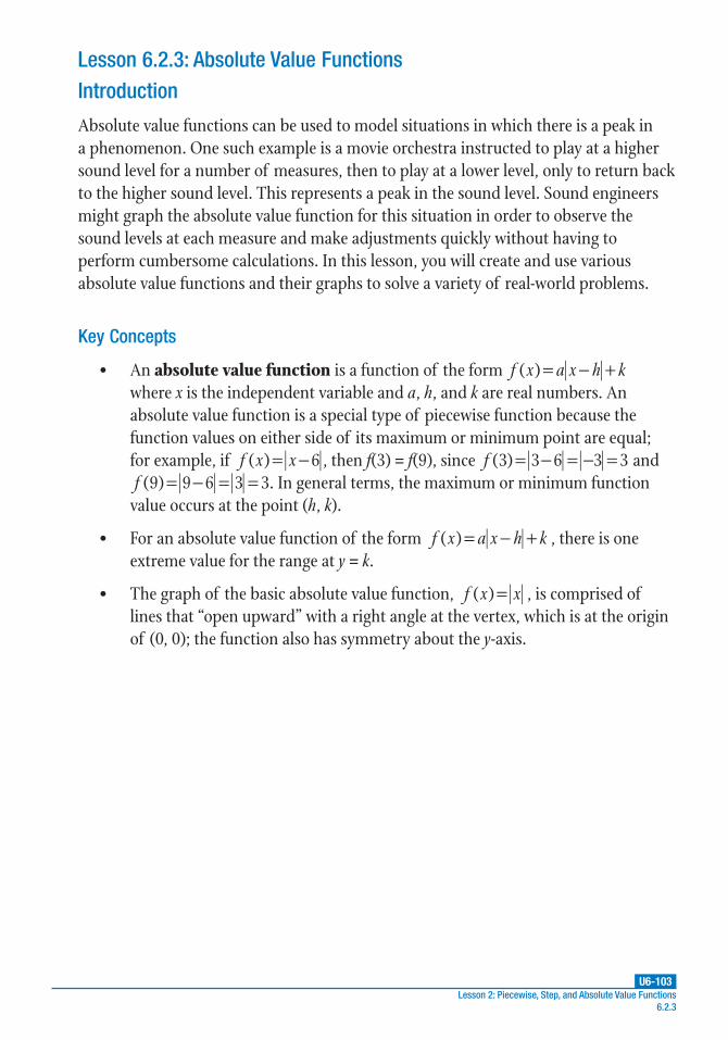
U6-103Lesson 2: Piecewise, Step, and Absolute Value Functions
6.2.3
Introduction
Absolute value functions can be used to model situations in which there is a peak in a phenomenon. One such example is a movie orchestra instructed to play at a higher sound level for a number of measures, then to play at a lower level, only to return back to the higher sound level. This represents a peak in the sound level. Sound engineers might graph the absolute value function for this situation in order to observe the sound levels at each measure and make adjustments quickly without having to perform cumbersome calculations. In this lesson, you will create and use various absolute value functions and their graphs to solve a variety of real-world problems.
Key Concepts
• An absolute value function is a function of the form f x a x h k( )= − + where x is the independent variable and a, h, and k are real numbers. An absolute value function is a special type of piecewise function because the function values on either side of its maximum or minimum point are equal; for example, if f x x( ) 6= − , then f(3) = f(9), since f (3) 3 6 3 3= − = − = and f (9) 9 6 3 3= − = = . In general terms, the maximum or minimum function
value occurs at the point (h, k).
• For an absolute value function of the form f x a x h k( )= − + , there is one extreme value for the range at y = k.
• The graph of the basic absolute value function, f x x( ) = , is comprised of lines that “open upward” with a right angle at the vertex, which is at the origin of (0, 0); the function also has symmetry about the y-axis.
Lesson 6.2.3: Absolute Value Functions
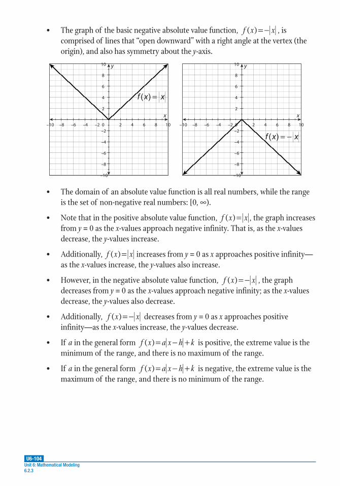
U6-104Unit 6: Mathematical Modeling 6.2.3
• The graph of the basic negative absolute value function, f x x( )=− , is comprised of lines that “open downward” with a right angle at the vertex (the origin), and also has symmetry about the y-axis.
–10 –8 –6 –4 –2 0 2 4 6 8 10
–10
–8
–6
–4
–2
2
4
6
8
10 y
x
f x x( ) =
–10 –8 –6 –4 –2 0 2 4 6 8 10
–10
–8
–6
–4
–2
2
4
6
8
10 y
x
f x x( ) = −
• The domain of an absolute value function is all real numbers, while the range is the set of non-negative real numbers: [0, ∞).
• Note that in the positive absolute value function, f x x( ) = , the graph increases from y = 0 as the x-values approach negative infinity. That is, as the x-values decrease, the y-values increase.
• Additionally, f x x( ) = increases from y = 0 as x approaches positive infinity—as the x-values increase, the y-values also increase.
• However, in the negative absolute value function, f x x( )=− , the graph decreases from y = 0 as the x-values approach negative infinity; as the x-values decrease, the y-values also decrease.
• Additionally, f x x( )=− decreases from y = 0 as x approaches positive infinity—as the x-values increase, the y-values decrease.
• If a in the general form f x a x h k( )= − + is positive, the extreme value is the minimum of the range, and there is no maximum of the range.
• If a in the general form f x a x h k( )= − + is negative, the extreme value is the maximum of the range, and there is no minimum of the range.

U6-105Lesson 2: Piecewise, Step, and Absolute Value Functions
6.2.3
• Graphing calculators can be an efficient way to graph absolute value functions. Follow the directions specific to your model.
On a TI-83/84:
Step 1: Press [Y=]. At [Y1], press [2ND][0] to bring up the Catalog menu. Select “abs(”. Enter the expression contained within the absolute value bars, using [X, T, θ, n] for x. Enter the remaining part of the expression by moving the cursor to the left and/or right of the absolute value bars. Enter additional absolute value functions on separate lines.
Step 2: Press [GRAPH]. Adjust the viewing window as needed.
On a TI-Nspire:
Step 1: Press the [home] key. Arrow down and over to the graphing icon and press [enter].
Step 2: Enter the expression at the bottom of the application, using x as the variable. Type “abs(x)” to enter an absolute value; for example, typing “abs(x+4)–5” is equivalent to the expression x 4 5+ − . Press [enter]. Adjust the viewing window as needed.

U6-106Unit 6: Mathematical Modeling 6.2.3
Guided Practice 6.2.3Example 1
Jonas rolls a basketball up a ramp and down the ramp’s other side. If the ball’s path were sketched on a coordinate plane, it would contain the points (0, 0), (10, 5), and (20, 0). Use the given points to write an absolute value function in the form f x a x h k( )= − + .
1. Determine the vertex (h, k) of the absolute value function.
Identify the variables h and k from the original problem. By the standard form of an equation of an absolute value graph, f x a x h k( )= − + , we know that the vertex (h, k) is the highest point of the graph of the absolute function. The highest point given in the original problem is (10, 5). Therefore, the vertex is (10, 5), with h = 10 and k = 5.
2. Use a given point and the values of h and k to solve for a.
The problem states that the ball travels upward, then downward. Since the path of the ball forms a shape that opens downward, we know that a is a negative number. Choose one of the given points to substitute into the general absolute value function, along with the values of h and k, to find a. A convenient point to use is (0, 0).
f x a x h k( )= − + Standard form of an absolute value function
f x a x( ) (10) (5)= − + Substitute 10 for h and 5 for k.
a(0) (0) 10 5= − + Substitute (0, 0) into the equation.
a0 10 5= − + Simplify.
a0 (10) 5= + Apply the absolute value.
–5 = 10a Subtract 5 from both sides.
a1
2=−
Divide and apply the Symmetric Property of Equality.
The value of a is 1
2− . As anticipated, it is a negative number.
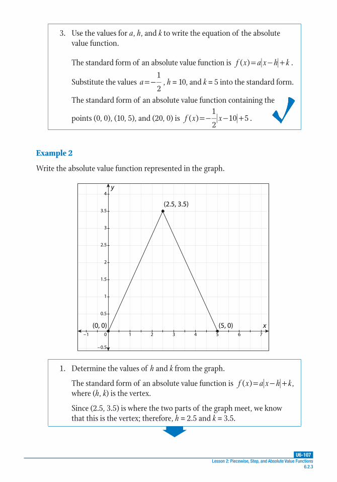
U6-107Lesson 2: Piecewise, Step, and Absolute Value Functions
6.2.3
3. Use the values for a, h, and k to write the equation of the absolute value function.
The standard form of an absolute value function is f x a x h k( )= − + .
Substitute the values a1
2=− , h = 10, and k = 5 into the standard form.
The standard form of an absolute value function containing the
points (0, 0), (10, 5), and (20, 0) is f x x( )1
210 5=− − + .
Example 2
Write the absolute value function represented in the graph.
–1 1 2 3 4 5 6 7
x
4
3.5
3
2.5
2
1.5
1
0.5
0
–0.5
y
(2.5, 3.5)
(0, 0) (5, 0)
1. Determine the values of h and k from the graph.
The standard form of an absolute value function is f x a x h k( )= − + , where (h, k) is the vertex.
Since (2.5, 3.5) is where the two parts of the graph meet, we know that this is the vertex; therefore, h = 2.5 and k = 3.5.

U6-108Unit 6: Mathematical Modeling 6.2.3
2. Determine the value of a.
Choose one of the given points to substitute into the general absolute value function, along with the values of h and k, to find a. A convenient point to use is (0, 0).
f x a x h k( )= − + Standard form for an absolute value function
f x a x( ) (2.5) (3.5)= − + Substitute 2.5 for h and 3.5 for k.
a(0) (0) 2.5 3.5= − + Substitute (0, 0) into the equation.
a0 2.5 3.5= − + Simplify.
0 = 2.5a + 3.5 Apply the absolute value.
–3.5 = 2.5a Subtract 3.5 from both sides.
a = –1.4Divide and apply the Symmetric Property of Equality.
The value of a is –1.4. A negative value for a means the graph opens downward, which corresponds with the provided graph.
3. Use the values for a, h, and k to write the equation of the absolute value function.
The standard form of an absolute value function is f x a x h k( )= − + . Substitute the values a = –1.4, h = 2.5, and k = 3.5 into this form.
The standard form of the absolute value function shown in the graph is f x x( ) 1.4 2.5 3.5=− − + .

U6-109Lesson 2: Piecewise, Step, and Absolute Value Functions
6.2.3
Example 3
Graph f x x( ) 6 1= + − by hand. Use the graph to identify the domain and the vertex.
1. Determine the values of h and k in the given function.
The standard form of an absolute value function is f x a x h k( )= − + , where the vertex is (h, k).
Identify the vertex of f x x( ) 6 1= + − by comparing the values in the given function to those of the standard form.
f x a x h k
f x x
( )
( ) 6 1
= − +
↓ ↓= + −
Note that the signs of the values in the given function that correspond to h and k are the opposite of the signs in the standard form. Rewrite the given function so that 6 and 1 have the same signs as h and k in the standard form.
f x x( ) 6 1= + − Given function
f x x( ) ( 6) ( 1)= − − + − Change the signs of 6 and 1 using operations.
x 6+ rewritten in standard form is x ( 6)− − ; therefore, h = –6.
1 rewritten in standard form is –1; therefore, k = –1.
The vertex (h, k) of the function f x x( ) 6 1= + − is (–6, –1).
2. Use the vertex to create a table of values.
The vertex is (–6, –1). Choose x-values that are less than and greater than x = –6 to find the coordinates of the points on either side of the vertex point (–6, –1).
For example, –8 and –7 are less than –6, and –5 and –4 are greater than –6.
(continued)

U6-110Unit 6: Mathematical Modeling 6.2.3
Substitute these values into the given function.
x ( ) 6 1f x x= + − y (x, y)
–8 f x( ) ( 8) 6 1= − + − 1 (–8, 1)
–7 f x( ) ( 7) 6 1= − + − 0 (–7, 0)
–6 f x( ) ( 6) 6 1= − + − –1 (–6, –1)
–5 f x( ) ( 5) 6 1= − + − 0 (–5, 0)
–4 f x( ) ( 4) 6 1= − + − 1 (–4, 1)
3. Plot the points from the table on a coordinate plane and sketch the graph.
The resulting graph of f x x( ) 6 1= + − should resemble the following.
–10 –8 –6 –4 –2 2 4 6 8 10
x
10
8
6
4
2
0
–2
–4
–6
–8
–10
y
4. Identify the domain and the vertex from the graph.
From the graph, notice that the function exists for all x-values, so the domain is all real numbers. The vertex point of the graph is (–6, –1), which confirms the result found mathematically.

U6-111Lesson 2: Piecewise, Step, and Absolute Value Functions
6.2.3
Example 4
Graph f x x( ) = , g x x( ) 5= + , and h x x( ) 5= using a graphing calculator. Compare the domains, intercepts, vertices, and symmetry.
1. Use a graphing calculator to graph each function.
Follow the directions appropriate to your model.
The graphed functions should resemble the following:
–10 –5 50 10 15 20
x
24
22
20
18
16
14
12
10
8
6
4
2
–2
y
h(x)
g(x)
f(x)
2. Compare the domains of the functions.
Look at the values of x for which the functions are defined. For each of the graphs, the lines are continuous as the values of x go from negative infinity to positive infinity.
Therefore, the domain for all three graphs is all real numbers.

U6-112Unit 6: Mathematical Modeling 6.2.3
3. Compare the x- and y-intercepts of each function.
f x x( ) = and h x x( ) 5= both have x- and y-intercepts at (0, 0). g x x( ) 5= + has a y-intercept at (0, 5), but no x-intercept.
4. Compare the vertices of each function.
For these graphs, the vertex will be the lowest point on the absolute value function.
f x x( ) = and h x x( ) 5= each have a vertex at (0, 0); g x x( ) 5= + has a vertex at (0, 5).
5. Compare the lines of symmetry of each function.
A line that goes through the vertex point of the absolute value graph is a line of symmetry.
The line x = 0 (the y-axis) is the line of symmetry for all three functions.
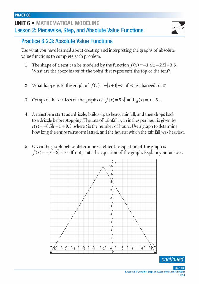
U6-113
PRACTICE
UNIT 6 • MATHEMATICAL MODELINGLesson 2: Piecewise, Step, and Absolute Value Functions
Lesson 2: Piecewise, Step, and Absolute Value Functions 6.2.3
Use what you have learned about creating and interpreting the graphs of absolute value functions to complete each problem.
1. The shape of a tent can be modeled by the function f x x( ) 1.4 2.5 3.5=− − + . What are the coordinates of the point that represents the top of the tent?
2. What happens to the graph of f x x( ) 1 3=− + − if –3 is changed to 3?
3. Compare the vertices of the graphs of f x x( ) 5= and g x x( ) 5= − .
4. A rainstorm starts as a drizzle, builds up to heavy rainfall, and then drops back to a drizzle before stopping. The rate of rainfall, r, in inches per hour is given by r t t( ) 0.5 1 0.5=− − + , where t is the number of hours. Use a graph to determine how long the entire rainstorm lasted, and the hour at which the rainfall was heaviest.
5. Given the graph below, determine whether the equation of the graph is f x x( ) 2 10=− − − . If not, state the equation of the graph. Explain your answer.
–12 –10 –8 –6 –4 –2 20 4 6 8
x
10
9
8
7
6
5
4
3
2
1
y
Practice 6.2.3: Absolute Value Functions
continued

U6-114
PRACTICE
UNIT 6 • MATHEMATICAL MODELINGLesson 2: Piecewise, Step, and Absolute Value Functions
Unit 6: Mathematical Modeling 6.2.3
6. What is the change in y-values for f x x( ) 2 3=− + + as x changes from 0 to 0.5?
7. A student’s grades slowly decline starting from the beginning of the semester, reach a low point, and then begin to improve by the end. What would need to be true about the shape of the graph of this absolute value function and the value of a in the equation?
8. What are the domain and vertex of the function f x x( ) 2= − ? How do they compare with those of the function g x x( ) 2= + ?
9. Compare the vertices of f x x( ) = and g x x( ) 2= + .
10. Compare the vertices and lines of symmetry of f x x( ) = and g x x( ) 2= .

Lesson 3: Working with Constraint Equations and Inequalities
UNIT 6 • MATHEMATICAL MODELING
U6-115Lesson 3: Working with Constraint Equations and Inequalities
6.3
Common Core Georgia Performance Standards
MCC9–12.A.CED.2★
MCC9–12.A.CED.3★
MCC9–12.A.CED.4★
Essential Questions
1. How are equations used to represent situations?
2. What does the solution for a system of equations represent?
3. What are constraints and how do they affect solutions?
4. How do you graph a system of linear inequalities?
5. How do you interpret the solution for a system of linear inequalities?
WORDS TO KNOW
boundary line a solid or dotted line that represents the edge of a linear inequality
boundary region a shaded area on a graph that represents a set of solutions to a linear inequality or system of linear inequalities; also called the feasible region
constraint a limit or restriction on the domain, range, and/or solutions of a mathematical or real-world problem
feasible region a shaded area on a graph that represents a set of solutions to a linear inequality or system of linear inequalities; also called the boundary region
feasible solution a set of acceptable solutions to a constraint equation, in the form (x, y); also known as a reasonable solution
U6-116Unit 6: Mathematical Modeling 6.3
inequality a mathematical statement that compares the value of an expression in one independent variable to the value of a dependent variable using the comparison symbols >, <, ≥, ≤, and ≠
intersection on a coordinate plane, the point at which the graphs of two or more equations or inequalities cross
linear inequality an inequality that has one or more variables to the first power and contains at least one of the following symbols: <, >, ≤, ≥, or ≠
ratio the relationship between two quantities; can be expressed in words, fractions, decimals, or as a percentage
reasonable solution a set of acceptable solutions to a constraint equation, in the form (x, y); also known as a feasible solution
substitution method solving one of a pair of equations for one of the variables and substituting that into the other equation
system of equations a set of equations with the same unknowns
system of inequalities a set of inequalities with the same unknowns
Recommended Resources
• Khan Academy. “Multiple Examples of Multiple Constraint Problems.”
http://www.walch.com/rr/00270
These video tutorials review creating a constraint equation, finding solutions, and interpreting the solutions in the context of problems. Each video includes an interactive transcript.
• MathIsFun.com. “Systems of Linear Equations.”
http://www.walch.com/rr/00271
This site provides a thorough explanation of systems of linear equations and how to interpret their solutions (or lack thereof ).
• OnlineMathLearning.com. “Represent Constraints (Equations, Inequalities).”
http://www.walch.com/rr/00272
This site offers five video tutorials on how to use linear equations and inequalities to create different scenarios that involve constraints.
U6-117Lesson 3: Working with Constraint Equations and Inequalities
6.3.1
Introduction
Constraint equations are used to model real-life situations that involve limits. Unlike other types of equations used for modeling, constraint equations account for restrictions that exist in a situation. For example, when projecting budgets in business, conditions or restrictions often exist on available time, space, and money.
When graphing a linear constraint equation, acceptable solutions will appear on the graphed line. Since a line has an infinite number of points, an infinite number of solutions work for that equation. A constraint equation shows what restrictions must be placed on the variables to identify solutions that reflect the real-world limits of the situation.
Key Concepts
• A constraint equation is an equation that expresses a restriction in the relationship between two quantities.
• A linear constraint equation is most often given in the form ax + by = c, where a, b, and c are constants, but can be rewritten in slope-intercept form, y = mx + b, where m is the slope and b is the y-intercept. Also, there is a ratio between the two quantities x and y, with a and b serving as conditions or restrictions set on x and y. A ratio is the relationship between two quantities, and can be expressed in words, fractions, decimals, or as a percentage.
• The graph of a linear constraint equation is a line whose points represent the feasible solutions (or reasonable solutions) of the equation. The acceptable solutions for a linear equation are given in the form (x, y).
• Recall that the domain is the set of all x-values that are valid for a given situation’s equation.
• A typical line graph for a constraint equation would show an x-intercept at (x, 0) if the line crosses the x-axis. Similarly, the line for a constraint equation would show a y-intercept at (0, y) if the line crosses the y-axis.
Lesson 6.3.1: Creating Constraint Equations
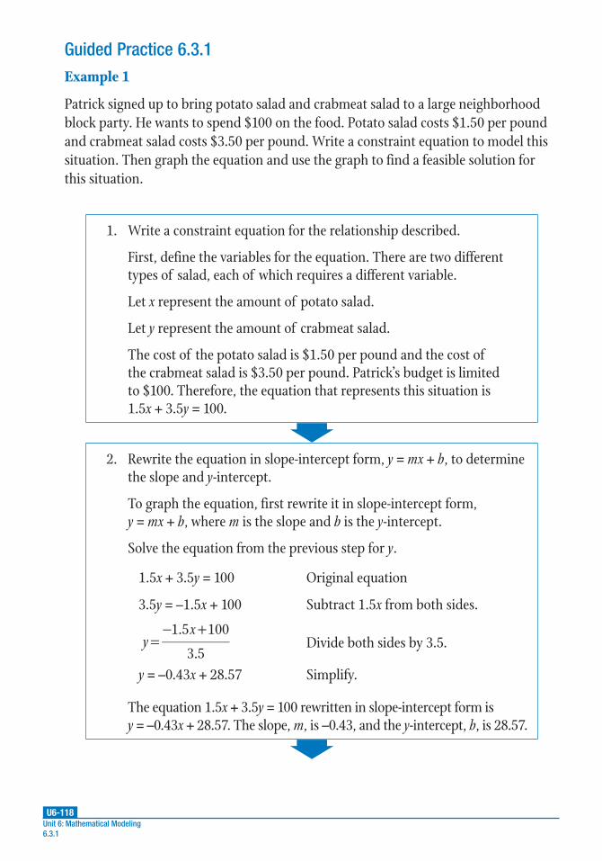
U6-118Unit 6: Mathematical Modeling 6.3.1
Guided Practice 6.3.1Example 1
Patrick signed up to bring potato salad and crabmeat salad to a large neighborhood block party. He wants to spend $100 on the food. Potato salad costs $1.50 per pound and crabmeat salad costs $3.50 per pound. Write a constraint equation to model this situation. Then graph the equation and use the graph to find a feasible solution for this situation.
1. Write a constraint equation for the relationship described.
First, define the variables for the equation. There are two different types of salad, each of which requires a different variable.
Let x represent the amount of potato salad.
Let y represent the amount of crabmeat salad.
The cost of the potato salad is $1.50 per pound and the cost of the crabmeat salad is $3.50 per pound. Patrick’s budget is limited to $100. Therefore, the equation that represents this situation is 1.5x + 3.5y = 100.
2. Rewrite the equation in slope-intercept form, y = mx + b, to determine the slope and y-intercept.
To graph the equation, first rewrite it in slope-intercept form, y = mx + b, where m is the slope and b is the y-intercept.
Solve the equation from the previous step for y.
1.5x + 3.5y = 100 Original equation
3.5y = –1.5x + 100 Subtract 1.5x from both sides.
yx1.5 100
3.5=− +
Divide both sides by 3.5.
y = –0.43x + 28.57 Simplify.
The equation 1.5x + 3.5y = 100 rewritten in slope-intercept form is y = –0.43x + 28.57. The slope, m, is –0.43, and the y-intercept, b, is 28.57.

U6-119Lesson 3: Working with Constraint Equations and Inequalities
6.3.1
3. Graph the result by hand or using a graphing calculator.
The graph should resemble the following.
10 20 30 40 50 60 70 80
x
40
38
36
34
32
30
28
26
24
22
20
18
16
14
12
10
8
6
4
20
–2
y
Notice that the graph includes negative values; however, it is important to note that given the scenario, the values should be restricted to the first quadrant, and should not include any negative values. This is because the constraint equation in this problem involves domains that are non-negative. For example, it would be impossible to purchase a negative amount of potato salad or crabmeat salad.
4. Use the graph to identify a feasible solution to the problem.
Pick any point on the line and identify the x- and y-coordinates. Approximate the coordinates if needed.
One possible solution would be (20, 20). This means that Patrick can buy 20 pounds of potato salad at $1.50 per pound, since $1.50(20) = $30, and 20 pounds of crabmeat salad at $3.50 per pound, since $3.50(20) = $70, for a total of $100 spent.
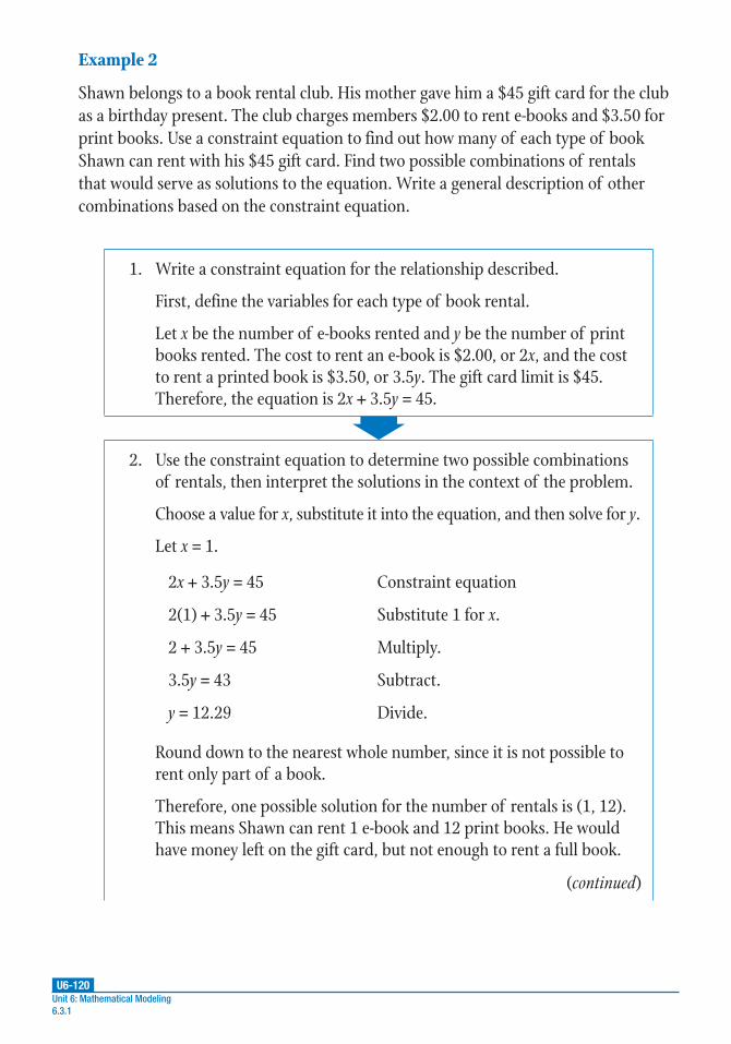
U6-120Unit 6: Mathematical Modeling 6.3.1
Example 2
Shawn belongs to a book rental club. His mother gave him a $45 gift card for the club as a birthday present. The club charges members $2.00 to rent e-books and $3.50 for print books. Use a constraint equation to find out how many of each type of book Shawn can rent with his $45 gift card. Find two possible combinations of rentals that would serve as solutions to the equation. Write a general description of other combinations based on the constraint equation.
1. Write a constraint equation for the relationship described.
First, define the variables for each type of book rental.
Let x be the number of e-books rented and y be the number of print books rented. The cost to rent an e-book is $2.00, or 2x, and the cost to rent a printed book is $3.50, or 3.5y. The gift card limit is $45. Therefore, the equation is 2x + 3.5y = 45.
2. Use the constraint equation to determine two possible combinations of rentals, then interpret the solutions in the context of the problem.
Choose a value for x, substitute it into the equation, and then solve for y.
Let x = 1.
2x + 3.5y = 45 Constraint equation
2(1) + 3.5y = 45 Substitute 1 for x.
2 + 3.5y = 45 Multiply.
3.5y = 43 Subtract.
y = 12.29 Divide.
Round down to the nearest whole number, since it is not possible to rent only part of a book.
Therefore, one possible solution for the number of rentals is (1, 12). This means Shawn can rent 1 e-book and 12 print books. He would have money left on the gift card, but not enough to rent a full book.
(continued)

U6-121Lesson 3: Working with Constraint Equations and Inequalities
6.3.1
Repeat this process with a new value for x. Let x = 10.
2x + 3.5y = 45 Constraint equation
2(10) + 3.5y = 45 Substitute 10 for x.
20 + 3.5y = 45 Multiply.
3.5y = 25 Subtract.
y = 7.14 Divide
After rounding down to the nearest whole number, another possible solution for the number of rentals is (10, 7). Shawn can rent 10 e-books and 7 print books and still have some money left on the gift card.
3. Describe other combinations based on the constraint equation.
In general, any integer point (x, y) below the line 2x + 3.5y = 45 would be a feasible combination of printed books and e-books Shawn can rent with his gift card.

U6-122Unit 6: Mathematical Modeling 6.3.1
Example 3
Ann is trying to decide whether to sign up for a new “pay as you go” cell phone plan. The plan charges $0.25 per minute for calls and $0.10 per text message, which includes all taxes and fees. She wants to spend no more than $100 monthly for cell service. Write the constraint equation and then graph the solution. Finally, determine the domain of the graph (minutes for calls) and interpret how it relates to this situation.
1. Write a constraint equation for the relationship described.
Let x be the number of minutes of calls made in a month, and let y be the number of texts sent in a month.
Calls cost $0.25 per minute, or 0.25x, and texts cost $0.10, or 0.1y. Ann’s total monthly budget is $100. Therefore, the equation is 0.25x + 0.1y = 100.
2. Rewrite the equation in slope-intercept form, y = mx + b, to determine the slope and y-intercept.
To graph the equation, first rewrite it in slope-intercept form, y = mx + b, where m is the slope and b is the y-intercept.
Solve 0.25x + 0.1y = 100 for y.
0.25x + 0.1y = 100 Original equation
0.1y = –0.25x + 100 Subtract 0.25x from both sides.
=− +
yx0.25 100
0.1Divide both sides by 0.1.
y = –2.5x + 1000 Simplify.
The equation 0.25x + 0.1y = 100 rewritten in slope-intercept form is y = –2.5x + 1000, where –2.5 is the slope and 1,000 is the y-intercept.
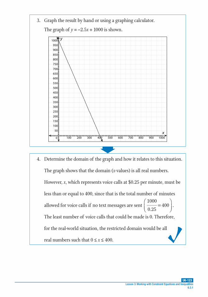
U6-123Lesson 3: Working with Constraint Equations and Inequalities
6.3.1
3. Graph the result by hand or using a graphing calculator.
The graph of y = –2.5x + 1000 is shown.
100 200 300 400 500 600 700 800 900 1000
x
1000
950
900
850
800
750
700
650
600
550
500
450
400
350
300
250
200
150
100
50
0
y
4. Determine the domain of the graph and how it relates to this situation.
The graph shows that the domain (x-values) is all real numbers.
However, x, which represents voice calls at $0.25 per minute, must be
less than or equal to 400, since that is the total number of minutes
allowed for voice calls if no text messages are sent 1000
0.25400=
.
The least number of voice calls that could be made is 0. Therefore,
for the real-world situation, the restricted domain would be all
real numbers such that 0 ≤ x ≤ 400.

U6-124Unit 6: Mathematical Modeling 6.3.1
Example 4
Marla is setting up a full-service hair salon and needs to plan the number of washing and styling stations the salon will have. She has $12,800 budgeted for washing and styling stations. Each washing station will cost $320, and each styling station will cost $400. Write the constraint equation for this situation, and use it to identify the intercepts of the graph. Explain what the intercepts mean in the context of the situation, and whether they represent reasonable solutions given the real-world constraints.
1. Write a constraint equation for the relationship described.
Let x be the number of washing stations and y be the number of styling stations.
The cost per washing station is $320, or 320x, and the cost per styling station is $400, or 400y. Marla’s budget is $12,800. Therefore, the equation is 320x + 400y = 12,800.
2. Use the constraint equation to identify the x- and y-intercepts.
To find the x-intercept, let y = 0, substitute this value into the constraint equation, and then solve for x.
320x + 400y = 12,800 Original equation
320x + 400(0) = 12,800 Substitute 0 for y.
320x = 12,800 Simplify.
x12,800
320= Divide both sides by 320.
x = 40 Simplify.
The x-intercept is (40, 0).(continued)

U6-125Lesson 3: Working with Constraint Equations and Inequalities
6.3.1
To find the y-intercept, let x = 0, substitute this value into the constraint equation, and then solve for y.
320x + 400y = 12,800 Original equation
320(0) + 400y = 12,800 Substitute 0 for x.
400y = 12,800 Simplify.
y12,800
400= Divide both sides by 400.
y = 32 Simplify.
The y-intercept is (0, 32).
3. Explain what the intercepts mean and whether they represent reasonable solutions given the context.
In this situation, the x-intercept (40, 0) means that Marla could buy 40 washing stations if she does not buy any styling stations. This is possible but unrealistic, because it is not likely that a salon would have washing stations but no styling stations.
Similarly, the y-intercept (0, 32) means that Marla could buy 32 styling stations if she does not buy any washing stations. This could make sense for a salon that does not offer hair washing, but since the original problem states that Marla plans a “full-service” hair salon, the implication is that the hairdressers would need to both wash and style hair. Therefore, neither intercept is a reasonable solution to the problem given the context.

U6-126
PRACTICE
UNIT 6 • MATHEMATICAL MODELINGLesson 3: Working with Constraint Equations and Inequalities
Unit 6: Mathematical Modeling 6.3.1
Use what you know about constraints to complete problems 1–4.
1. Daniel’s grandfather often complains about how he used to be able to buy a huge lunch of 3 hamburgers and 2 fish sandwiches for only $7.35. Write a constraint equation to model this situation.
2. Explain why the domain of the equation in problem 2 cannot be less than or equal to 0 in terms of the situation.
3. Charlotte purchased 2 pairs of tights and 4 pairs of socks for a total of $18.48 at an outlet store. If the cost of the 2 pairs of tights was equal to the cost of the 4 pairs of socks, how much did each individual pair of tights and socks cost?
4. Two people rent a moving truck from the same company. The moving company charges per day, with additional charges for each mile. The first person pays $1,845 to move 2,060 miles over 5 days, and the second person pays $840 to move 880 miles over 3 days. Write two equations that would represent the constraints in this situation.
Use the given information to complete problems 5–7.
Adelle and her friend Chrissy went on a hike. They walked at a rate of 3 miles per hour. After a while, they realized it was getting dark so they ran back at 6 mph. When they got back, they had walked and run a total of 12 miles.
5. Write a constraint equation for the situation described, using w for the number of hours they walked and r for the number of hours they ran.
6. Find two reasonable solutions that would satisfy the constraint equation.
7. Graph the equation and label the solutions from problem 6 on the graph.
Practice 6.3.1: Creating Constraint Equations
continued

U6-127
PRACTICE
UNIT 6 • MATHEMATICAL MODELINGLesson 3: Working with Constraint Equations and Inequalities
Lesson 3: Working with Constraint Equations and Inequalities 6.3.1
Use the given information to complete problems 8–10.
Robin invested $27,000 in two saving accounts. One pays 10% annual interest, and the other pays 12% annual interest. He invested $12,500 in the 10% account, and $14,500 in the 12% account. At the end of the first year, his combined total return from the two accounts was $2,990.
8. Write two constraint equations to model Robin’s investment.
9. Graph the equations you wrote for problem 8.
10. Identify and explain the domain and intercepts of the graph.

U6-128Unit 6: Mathematical Modeling 6.3.2
Introduction
Inequalities are mathematical statements that compare the value of an expression in one independent variable to the value of a dependent variable using the comparison symbols >, <, ≥, ≤, and ≠. Like linear equations, inequalities are also used to model a variety of real-life situations that involve restrictions or constraints.
Key Concepts
• A linear inequality is an inequality that has one or more variables to the first power and contains at least one inequality symbol.
• A linear inequality can be an individual mathematical statement or two or more statements presented as a system—that is, a set of more than one equation or inequality with the same unknowns. Each mathematical statement represents a restriction expressed in the situation, whether individually or in a system. Each statement uses inequality signs to represent words such as “less than” and “greater than” in the situation presented. The following table summarizes these inequality symbols and the wording they represent.
Symbol Meaning> greater than, more than< less than≥ greater than or equal to, at least≤ less than or equal to, at most
• The graph of a linear inequality is similar to that of a linear equation, but the line appears as either solid or dashed depending on the inequality sign used. This dashed or solid line that represents the edge of a linear inequality is called a boundary line. In a constraint inequality context, the boundary line denotes the limit of the feasible region or boundary region of acceptable solutions that satisfy the constraint.
• For example, if the boundary line is solid, the inequality contains either ≤ or ≥. On the other hand, if the boundary line is dashed, the inequality contains either < or >. On a graph, the boundary/feasible region is shaded; such shading shows on which side of the boundary line the acceptable solutions to the system can be found.
• The x- and y-intercepts of a constrained inequality are also similar to those of a linear constraint equation in that they indicate the points where the line crosses the x- and y-axes, respectively.
Lesson 6.3.2: Creating Constraint Inequalities

U6-129Lesson 3: Working with Constraint Equations and Inequalities
6.3.2
• A system of equations is a set of equations that have the same unknowns.
For example, x y
x y
6
–3 2
+ =+ =
is a system of equations using the variables x and y,
grouped together with a brace, {.
• Similarly, a system of inequalities is a set of inequalities with the same
unknowns. Generally, the system contains two or more linear inequalities
in two or more unknown variables, which represent separate constraints or
restrictions for the same situation. Systems of linear inequalities are often
written together in a single brace, such as x y
y x
3 2 7
5
+ ≤+ >
.
• The solution to a system of inequalities is the set of domain values that satisfy both inequalities.
• The solutions to a set of linear inequalities or equations in two variables x and y can be found using substitution. The substitution method requires solving one of the equations in the set for one of the variables, then substituting that value into the other equation to solve for the other variable.
• The intersection of the inequalities in a system is the point on a graph where the lines cross. (Note: Not all systems of linear inequalities have a point of intersection.)
• The graph of a system of linear inequalities is similar to that of a linear inequality in that there are boundaries and shaded regions. The only difference is that the graph of a system shows two or more lines. Each line is solid or dashed depending on the inequality used in the original inequalities.
• In addition, shaded regions represent linear inequalities and correspond to the direction of the inequality symbols in the original inequality statement. For instance, linear inequality statements when solved for y that contain “less than” inequalities (<, ≤) are shaded under the line, whereas “greater than” inequalities (>, ≥) are shaded above the line on the graph. Shaded regions of systems of inequalities will often overlap when indicating where feasible solutions are on the graph.

U6-130Unit 6: Mathematical Modeling 6.3.2
Guided Practice 6.3.2Example 1
Willow is selling bracelets for $5 each and necklaces for $7 each. If she sold 10 bracelets, determine how many necklaces she would need to sell in order to make at least $100.
1. Define the variables in this situation.
Let b be the number of bracelets sold and n be the number of necklaces sold.
2. Write the inequality that represents the condition in this situation.
The cost of a bracelet is $5, or 5b, and the cost of a necklace is $7, or 7n.
Willow wants to make at least $100, which includes $100 and any amount above that. Therefore, the inequality is 5b + 7n ≥ 100.
3. Determine how many necklaces Willow would need to sell to reach her goal if she sold 10 bracelets.
To determine the number of necklaces she would need to sell, let b = 10 and solve 5b + 7n ≥ 100 for n.
5b + 7n ≥ 100 Original inequality
5(10) + 7n ≥ 100 Substitute 10 for b.
50 + 7n ≥ 100 Multiply.
7n ≥ 50 Subtract 50 from both sides.
n ≥ 7.1 Divide by 7 on both sides.
Round n to the nearest whole necklace: n ≥ 8.
Confirm your results by substituting 10 for b and 8 for n into the inequality to see if the result is a true statement.
5b + 7n ≥ 100
5(10) + 7(8) ≥ 100
50 + 56 ≥ 100
106 ≥ 100
This is a true statement.
If Willow sold 10 bracelets, she would need to sell 8 necklaces to make at least $100.
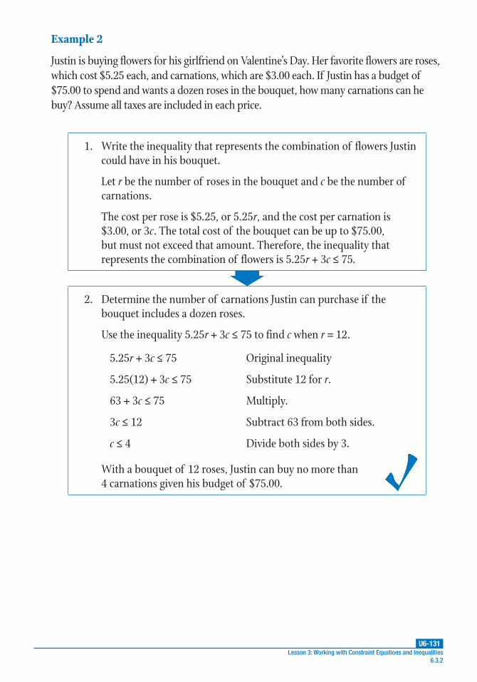
U6-131Lesson 3: Working with Constraint Equations and Inequalities
6.3.2
Example 2
Justin is buying flowers for his girlfriend on Valentine’s Day. Her favorite flowers are roses, which cost $5.25 each, and carnations, which are $3.00 each. If Justin has a budget of $75.00 to spend and wants a dozen roses in the bouquet, how many carnations can he buy? Assume all taxes are included in each price.
1. Write the inequality that represents the combination of flowers Justin could have in his bouquet.
Let r be the number of roses in the bouquet and c be the number of carnations.
The cost per rose is $5.25, or 5.25r, and the cost per carnation is $3.00, or 3c. The total cost of the bouquet can be up to $75.00, but must not exceed that amount. Therefore, the inequality that represents the combination of flowers is 5.25r + 3c ≤ 75.
2. Determine the number of carnations Justin can purchase if the bouquet includes a dozen roses.
Use the inequality 5.25r + 3c ≤ 75 to find c when r = 12.
5.25r + 3c ≤ 75 Original inequality
5.25(12) + 3c ≤ 75 Substitute 12 for r.
63 + 3c ≤ 75 Multiply.
3c ≤ 12 Subtract 63 from both sides.
c ≤ 4 Divide both sides by 3.
With a bouquet of 12 roses, Justin can buy no more than 4 carnations given his budget of $75.00.
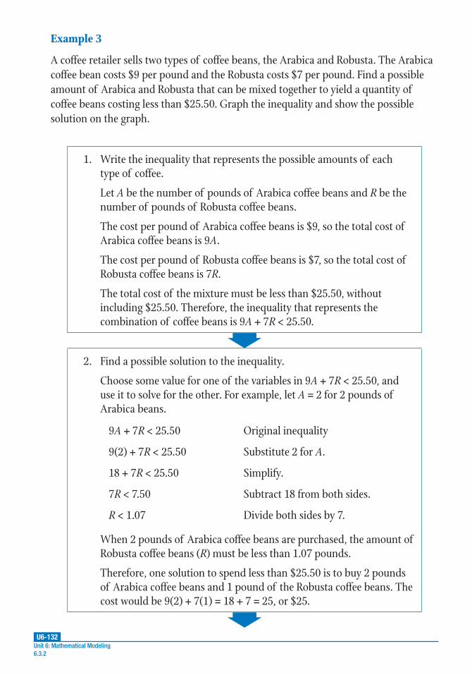
U6-132Unit 6: Mathematical Modeling 6.3.2
Example 3
A coffee retailer sells two types of coffee beans, the Arabica and Robusta. The Arabica coffee bean costs $9 per pound and the Robusta costs $7 per pound. Find a possible amount of Arabica and Robusta that can be mixed together to yield a quantity of coffee beans costing less than $25.50. Graph the inequality and show the possible solution on the graph.
1. Write the inequality that represents the possible amounts of each type of coffee.
Let A be the number of pounds of Arabica coffee beans and R be the number of pounds of Robusta coffee beans.
The cost per pound of Arabica coffee beans is $9, so the total cost of Arabica coffee beans is 9A.
The cost per pound of Robusta coffee beans is $7, so the total cost of Robusta coffee beans is 7R.
The total cost of the mixture must be less than $25.50, without including $25.50. Therefore, the inequality that represents the combination of coffee beans is 9A + 7R < 25.50.
2. Find a possible solution to the inequality.
Choose some value for one of the variables in 9A + 7R < 25.50, and use it to solve for the other. For example, let A = 2 for 2 pounds of Arabica beans.
9A + 7R < 25.50 Original inequality
9(2) + 7R < 25.50 Substitute 2 for A.
18 + 7R < 25.50 Simplify.
7R < 7.50 Subtract 18 from both sides.
R < 1.07 Divide both sides by 7.
When 2 pounds of Arabica coffee beans are purchased, the amount of Robusta coffee beans (R) must be less than 1.07 pounds.
Therefore, one solution to spend less than $25.50 is to buy 2 pounds of Arabica coffee beans and 1 pound of the Robusta coffee beans. The cost would be 9(2) + 7(1) = 18 + 7 = 25, or $25.

U6-133Lesson 3: Working with Constraint Equations and Inequalities
6.3.2
3. Graph the inequality using technology.
Follow the instructions appropriate to your calculator model.
On a TI-83/84:
Note: Directions differ for the TI-83 and TI-84.
Step 1: For the TI-83, press [MODE]. Use the arrow keys and [ENTER] to select “Dot,” then “Simul.” For the TI-84, press [APPS], then arrow down to select 7: Inequalz. Press [ENTER] twice. The menu for inequalities will appear.
Step 2: Press [Y=]. Enter the inequality at Y1. To select the appropriate inequality symbol:
• On the TI-83, press [2ND][TEST] to bring up a menu of inequality symbols.
• On the TI-84, arrow left to highlight the equal sign at Y1, which will bring up a menu of symbols on the bottom of the screen. Press [ALPHA] plus the function button ([F1]–[F5]) that’s immediately below the symbol you want to insert. Arrow right to enter the rest of the inequality.
Step 3: Press [GRAPH]. Press [WINDOW] to adjust the graph’s axes, if needed.
On a TI-Nspire:
Step 1: Press [home]. Arrow over to the graphing icon, the second icon from the left, and press [enter].
Step 2: At f1(x), enter the inequality using the appropriate symbols. Press [enter]. Note: The inequality needs to be entered in slope-intercept form.
Step 3: To adjust the window settings, press [menu], then select 4: Window/Zoom.
(continued)
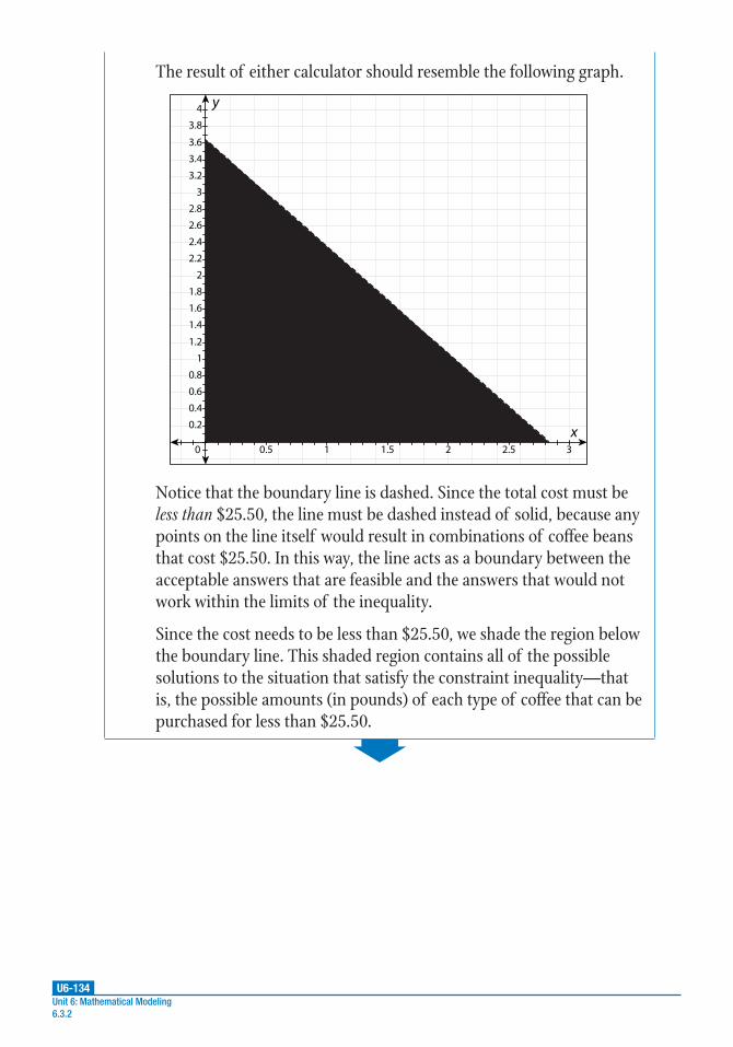
U6-134Unit 6: Mathematical Modeling 6.3.2
The result of either calculator should resemble the following graph.
0.5 1 1.5 2 2.5 3
x
4
3.8
3.6
3.4
3.2
3
2.8
2.6
2.4
2.2
2
1.8
1.6
1.4
1.2
1
0.8
0.6
0.4
0.2
y
0
Notice that the boundary line is dashed. Since the total cost must be less than $25.50, the line must be dashed instead of solid, because any points on the line itself would result in combinations of coffee beans that cost $25.50. In this way, the line acts as a boundary between the acceptable answers that are feasible and the answers that would not work within the limits of the inequality.
Since the cost needs to be less than $25.50, we shade the region below the boundary line. This shaded region contains all of the possible solutions to the situation that satisfy the constraint inequality—that is, the possible amounts (in pounds) of each type of coffee that can be purchased for less than $25.50.
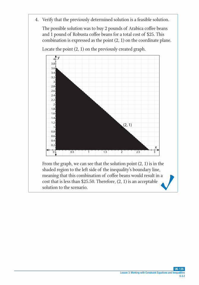
U6-135Lesson 3: Working with Constraint Equations and Inequalities
6.3.2
4. Verify that the previously determined solution is a feasible solution.
The possible solution was to buy 2 pounds of Arabica coffee beans and 1 pound of Robusta coffee beans for a total cost of $25. This combination is expressed as the point (2, 1) on the coordinate plane.
Locate the point (2, 1) on the previously created graph.
0.5 1 1.5 2 2.5 3
x
4
3.8
3.6
3.4
3.2
3
2.8
2.6
2.4
2.2
2
1.8
1.6
1.4
1.2
1
0.8
0.6
0.4
0.2
y
0
(2, 1)
From the graph, we can see that the solution point (2, 1) is in the shaded region to the left side of the inequality’s boundary line, meaning that this combination of coffee beans would result in a cost that is less than $25.50. Therefore, (2, 1) is an acceptable solution to the scenario.

U6-136
PRACTICE
UNIT 6 • MATHEMATICAL MODELINGLesson 3: Working with Constraint Equations and Inequalities
Unit 6: Mathematical Modeling 6.3.2
Use the following information to complete problems 1–3.
It’s Lindsay’s turn to provide snacks for her scout troop’s next meeting. She is planning to purchase bags of fruit for $5 each and bags of popcorn for $1 each. She only has $20 to spend. (Assume that all prices include tax.)
1. What inequality could be used to determine the combination of purchases needed?
2. Explain two possible combinations of popcorn and fruit purchases given the budget of $20.
3. Individually, what is the smallest amount of each item that she can purchase? Explain.
Use the following information to complete problems 4 and 5.
Bradley and Jennie own a pet day spa for dogs and cats. Up to 8 hours of each workday is spent feeding and playing with the animals. In terms of feeding times, the cats will require 12 minutes per day and the dogs will require 20 minutes per day. In terms of playtime, the cats need 16 minutes per day, while the dogs need 20 minutes per day. (Assume that the couple will spend 50% of the time feeding and 50% of the time playing.)
4. Write an inequality to reflect the time spent feeding the animals. Then, write an inequality for the time spent playing with them.
5. Graph and shade the solution set for each constraint inequality.
Practice 6.3.2: Creating Constraint Inequalities
continued
U6-137
PRACTICE
UNIT 6 • MATHEMATICAL MODELINGLesson 3: Working with Constraint Equations and Inequalities
Lesson 3: Working with Constraint Equations and Inequalities 6.3.2
Use the following information to complete problems 6–8.
Wallace sells appliances at a local store. He earns a commission of $60 for each washing machine he sells and $130 for each refrigerator he sells.
6. List the variables for this situation.
7. Write a constraint inequality for this scenario if Wallace wants to make a commission of $1,000 or more.
8. Use the constraint inequality from problem 7 to determine the intercepts mathematically. Explain what the intercepts mean in terms of how many washing machines and refrigerators Wallace must sell in order to earn his desired commission.
Use what you have learned about creating constraint equations and inequalities to complete problems 9 and 10.
9. A photographer sells $20 photo albums and $50 framed photos at a craft fair. If she sells twice as many albums as photos, what combination of products does she need to sell in order to make at least $200 at the fair?
10. Jamie is looking for loose coins in his couch to purchase a pack of chewing gum for $1.25. He found 10 dimes and quarters. Write a system of equations to determine how many dimes and quarters he must find to have at least $1.25. How many dimes and quarters must he find?

U6-138Unit 6: Mathematical Modeling 6.3.3
Introduction
Mathematical formulas that involve exponents, logarithms, powers, and roots have constraints on the values that can be assigned or associated with two or more variables. Real-world formulas involving measurements like area, length, time, and volume have additional restraints, whereas others (such as current, direction, and voltage) can have positive and negative values in addition to the limits imposed by real-world relationships. Rearranging variables in a formula can result in changes to these constraints, so the result of rearranging variables has to be checked and redefined in those cases. Formulas can often be analyzed and visualized in the same way that equations and functions can, and the data resulting from formulas can be presented as data in tables or in graphs.
Key Concepts
• A formula relates two or more variables in a mathematical or a real-world problem context.
• The values of the variables in a formula can be constrained or limited by
mathematical or real-world conditions. For example, the formula A bh1
2= for
the area of a triangle contains three quantities that are positive. If a triangle is
graphed on a coordinate plane and its orientation on the plane results in either
b or h being assigned a negative value, then the other variable must also be
assigned a negative value so that the area of the triangle is positive.
Lesson 6.3.3: Rearranging Formulas

U6-139Lesson 3: Working with Constraint Equations and Inequalities
6.3.3
• Rearranging a formula can leave the constraints on variable values the same
or it can change them. For example, in the distance-rate-time formula d = rt,
time is constrained by the condition t ≥ 0, with t = 0 signifying the time at
which motion begins. The formula can be rewritten as rd
t= ; however, r
d
t=
is undefined at t = 0, so in this case t > 0. This corresponds to the real-world
condition that r ≠ 0 only when t ≠ 0, since at t = 0, there is no distance covered
and no motion.
• Formulas can be rearranged to express one or more variables in terms of another variable. A rearranged formula can reduce the number of variables to be calculated.
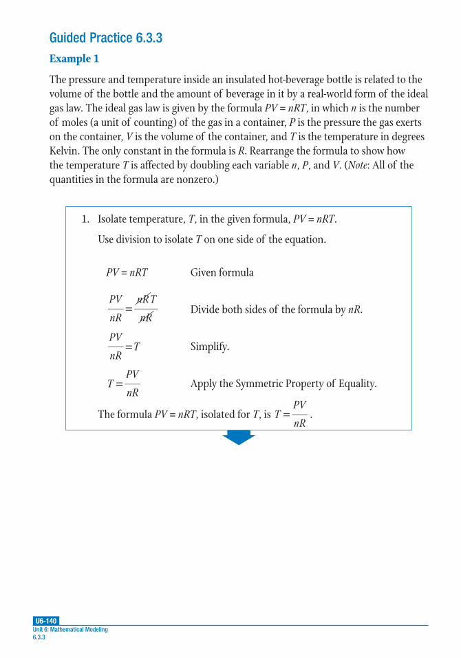
U6-140Unit 6: Mathematical Modeling 6.3.3
Guided Practice 6.3.3Example 1
The pressure and temperature inside an insulated hot-beverage bottle is related to the volume of the bottle and the amount of beverage in it by a real-world form of the ideal gas law. The ideal gas law is given by the formula PV = nRT, in which n is the number of moles (a unit of counting) of the gas in a container, P is the pressure the gas exerts on the container, V is the volume of the container, and T is the temperature in degrees Kelvin. The only constant in the formula is R. Rearrange the formula to show how the temperature T is affected by doubling each variable n, P, and V. (Note: All of the quantities in the formula are nonzero.)
1. Isolate temperature, T, in the given formula, PV = nRT.
Use division to isolate T on one side of the equation.
PV = nRT Given formula
PV
nR
nR T
nR= Divide both sides of the formula by nR.
PV
nRT= Simplify.
TPV
nR= Apply the Symmetric Property of Equality.
The formula PV = nRT, isolated for T, is TPV
nR= .
U6-141Lesson 3: Working with Constraint Equations and Inequalities
6.3.3
2. Determine how T is affected in the rearranged formula if n is doubled and P and V stay the same.
We are given that R is a constant, so it will not be affected by changes to the other variables.
Let the original value of n be n1. If n1 is doubled, the resulting value of n is 2n1.
Write the revised ideal gas law from step 1 for both conditions.
Formula rewritten for n1 (the original value of n):
TPV
n R11
=
Formula rewritten for 2n1 (twice the original value of n):
TPV
n R221
=
Factor out 1
2 from T
PV
n R221
= :
TPV
n R
1
221
= •
Notice that T2 is half of T1. In other words, doubling the value of n reduces the temperature by half. In general, increasing n will decrease T if P and V stay the same.

U6-142Unit 6: Mathematical Modeling 6.3.3
3. Determine how T is affected in the rearranged formula if P is doubled and n and V stay the same.
Let the original value of P be P1. If P1 is doubled, the resulting value of P is 2P1.
Write the revised ideal gas law from step 1 for both conditions.
Formula rewritten for P1 (the original value of P):
TP V
nR11=
Formula rewritten for 2P1 (twice the original value of P):
TP V
nR
22
1=
Factor out 2 from TP V
nR
22
1= :
TP V
nR22
1= •
Notice that T2 is twice T1. In other words, doubling the value of P doubles the temperature. In general, increasing P increases T if n and V stay the same.
4. Determine how T is affected in the rearranged formula if V is doubled and n and P stay the same.
Note that V, like P, is a factor of the numerator of the formula TPV
nR= .
Since both V and P are in the numerator, changes in the volume, V, would have the same effect on temperature, T, as changes in pressure, P. In other words, if we were to double the volume instead of the pressure, the temperature would still be doubled.
Therefore, increasing V increases T if n and P stay the same.

U6-143Lesson 3: Working with Constraint Equations and Inequalities
6.3.3
Example 2
The distance, d, an object moves in one direction can be described by the formula
d vt at1
22= + , in which v is the velocity of the object when timing starts, a is the
acceleration of the object when timing starts, t is the duration of the motion, and d
is the initial distance of the object relative to some arbitrary reference point (e.g., the
origin on a coordinate plane) when the timing starts. Rearrange the formula for d so
that it can be solved for t using the quadratic formula, xb b ac
a
4
2
2
=− ± −
. In this
problem, the quantities a, d, and v are constants that can be positive, negative, or 0.
Apply the condition t > 0 to the resulting values of t and interpret the result(s) for
real-world motion if the following values are given: a = –2 meters per second squared,
d = 10 meters from a reference point, and v = 5 meters per second. Describe the
motion of the object using these values.
1. Rewrite the given formula for d so that all of the terms are one side of the equation.
Rewriting the formula so all terms are on one side of the equation corresponds to having 0 on one side of the equation. Results that are in the form ax2 + bx + c = 0 reveal the values to be substituted into the quadratic formula.
d vt at1
22= + Given equation
at vt d01
22= + − Subtract d from both sides of the equation.
at vt d0 2 22= + − Multiply both sides of the equation by 2.
at vt d2 2 02 + − = Apply the Symmetric Property of Equality.
at2 + 2vt – 2d = 0 is a quadratic in the form ax2 + bx + c = 0.
U6-144Unit 6: Mathematical Modeling 6.3.3
2. Identify the values of the resulting equation that correspond to a, b, c, and x in the quadratic formula.
The quadratic formula is xb b ac
a
4
2
2
=− ± −
. For the equation
at2 + 2vt – 2d = 0, a = a, b = 2v, c = –2d, and x = t.
3. Use the quadratic formula and the values determined in the previous step to write an equation that can be solved for t.
xb b ac
a
4
2
2
=− ± −
Quadratic formula
tv v a d
a( )
(2 ) (2 ) 4( )( 2 )
2( )
2
=− ± − − Substitute a for a, 2v for b, –2d
for c, and t for x.
tv
a
v ad
a
4 8
2
2
=− ±+
Simplify.
tv
a
v ad
a
2(2 4 )
2
2
=− ±+ Factor out 2 from under the
radical sign.
tv
a
v ad
a
22
=− ±+
Divide.
The resulting equation is tv
a
v ad
a
22
=− ±+
.
4. Apply the real-world condition t > 0 to the “positive” result of the simplified quadratic equation.
Taking the positive result of the radical expression of the inequality
v
a
v ad
a
20
2
− ±+
> yields v
a
v ad
a
20
2
− ++
> .
v
a
v ad
a
20
2
− ++
> simplifies to v ad
a
v
a
22 +> .
This result can also be interpreted on the basis of the signs of the quantities a, d, and v. The radical sign also places a mathematical constraint on the relationship of d to v: v2 + 2ad ≥ 0 or v2 ≥ –2ad. Therefore, a < 0, v > 0, and d < 0.

U6-145Lesson 3: Working with Constraint Equations and Inequalities
6.3.3
5. Apply the real-world condition t > 0 to the “negative” result of step 3.
Taking the negative result of the radical expression of the inequality
v
a
v ad
a
20
2
− ±+
> yields v
a
v ad
a
20
2
− −+
> .
v
a
v ad
a
20
2
− −+
> simplifies to v ad
a
v
a
22 +< .
This result can also be interpreted on the basis of the signs of the quantities a, d, and v. The radical sign also places a mathematical constraint on the relationship of d to v: v2 + 2ad > 0 or v2 ≥ –2ad. Therefore, a < 0, v > 0, and d < 0.
6. Apply the real-world condition t > 0 to the “negative” result of step 3.
Taking the negative result of the radical expression of the inequality
v
a
v ad
a
20
2
− ±+
> yields v
a
v ad
a
20
2
− −+
> .
v
a
v ad
a
20
2
− −+
> simplifies to v ad
a
v
a
22 +< .
This result can also be interpreted on the basis of the signs of the quantities a, d, and v. The radical sign also places a mathematical constraint on the relationship of d to v: v2 + 2ad > 0 or v2 ≥ –2ad. Therefore, a < 0, v > 0, and d < 0.
U6-146Unit 6: Mathematical Modeling 6.3.3
7. Find t for the given values of a = –2 meters per second squared, d = 10 meters from a reference point, and v = 5 meters per second. Describe the motion of the object using these values.
Substitute these values into the simplified quadratic equation for t from step 3.
tv
a
v d
a
22
=− ±+
Simplified quadratic equation
t(5)
( 2)
(5) 2(10)
( 2)
2
=−−
±+−
Substitute –2 for a, 10 for d, and 5 for v.
t 2.545
2= ± Simplify.
t 2.5 1.5 5= ±
t ≈ –0.85 or t ≈ 5.85
These results give t ≈ –0.85 or t ≈ 5.85. Since t > 0, only the positive value for t is relevant.
Since only the positive value for t is relevant, the relationships found in step 4 for the positive radical expression should apply: a < 0 and v > 0.
Note that the given value for a is less than 0 and the given value for v is greater than 0, which follows the pattern of the restrictions on a and v.
U6-147Lesson 3: Working with Constraint Equations and Inequalities
6.3.3
8. Use the value of t found in the previous step to calculate d and compare it to the conditions in step 6. Interpret the result for d.
Remember that for the positive radical expression, the value of d for a < 0 and v > 0 should be given by d < 0.
d vt at1
22= + Original formula
d (5)(5.85)1
2( 2)(5.85)2≈ + − Substitute –2 for a, 5.85 for t, and
5 for v.
d ≈ –4.97 Simplify.
This value of d meets the criteria that d < 0.
Interpreting these values in the context of the problem, the object started out at 10 meters in a positive direction from the reference point. The acceleration and velocity result in motion that takes the object back (a negative distance) toward the reference point by almost 5 meters.

U6-148Unit 6: Mathematical Modeling 6.3.3
Example 3
The formula for a standard earthquake-body wave scale, mb, is given by
mA
TQb log=
+ , in which A is the amplitude of the ground motion in microns
(10–6 meter), T is the period of the wave, and Q is a correction constant. Determine a
formula for the frequency of the earthquake wave if the frequency F is defined as the
reciprocal of the wave period. Rearrange the formula to find the range of F values for
when the range of T values is [4, 5] seconds. Then, rearrange the formula to find the
range of values of A for when the range of values of mb is [6, 9], the range of T values
is [4, 5] seconds, and Q = 2.
1. Substitute an expression for F in place of T in the formula.
Frequency F can be written as FT
1= . The argument of the logarithm
A
T can be written as A
T
1
. Therefore, the argument of the
logarithm can be written as AF.
mA
TQb log=
+ Original formula
mb = log (AF) + Q Substitute AF for A
T.
The formula, using F in place of T, is mb = log (AF) + Q.

U6-149Lesson 3: Working with Constraint Equations and Inequalities
6.3.3
2. Use the definition of the logarithm to rewrite the formula with an exponential term. Then, solve it for F.
Isolate the logarithm from the rest of the formula, then simplify the result and solve it for F.
mb = log (AF) + Q Modified formula
mb – Q = log (AF) Subtract Q from both sides.
AFm Qb10 =− Definition of the logarithm
AFm
Q
b10
10= Simplify the exponential term.
FA
m
Q
b10
•10= Divide both sides by A.
The rewritten formula is FA
m
Q
b10
•10= .
3. Use the relationship between the period and the frequency to calculate the range of frequency values.
The period T is related to the frequency F by the relationship FT
1= .
If the range of T is [4, 5] seconds, then the range of F values is the
reciprocal of the period interval values, or 1
5,
1
4
.
U6-150Unit 6: Mathematical Modeling 6.3.3
4. Write the formula for the earthquake-magnitude scale so that the factors with known values are isolated from A.
To find the range of values of A for when the range of values of mb
is [6, 9] and Q = 2, first substitute 2 for Q in the rewritten formula,
FA
m
Q
b10
•10= , and then rearrange the formula so that it’s in terms of A.
FA
m
Q
b10
•10= Rewritten formula
FA
mb10
•10( 2)= Substitute 2 for Q.
FA
mb10 2
=−
Simplify using the rules of exponents.
AF mb10 2= − Multiply both sides by A.
AF
mb10 2
=−
Divide both sides by F.
A
T
mb101
2
=
−
Substitute T
1 for F.
A T mb•10 2= − Simplify.
The formula, written in terms of A when Q = 2, is A T mb•10 2= − .
U6-151Lesson 3: Working with Constraint Equations and Inequalities
6.3.3
5. Use the result of the previous step to write the maximum and minimum values of the range of values for A.
Use the formula, A T mb•10 2= − , to determine the minimum and maximum values using the given ranges of T and mb.
The range values for T are given as [4, 5], so the minimum value for T is 4 and the maximum value is 5.
The range values for mb are given as [6, 9]. Therefore, the minimum value for mb is 6 and the maximum value is 9.
Substitute the minimum values, T = 4 and mb = 6:
A T mb•10minimum2= − Formula for the minimum value of A
A 4 •10minimum6 2( )= ( )− Substitute 4 for T and 6 for mb.
A 4•10minimum4= Simplify.
The minimum value of A is 4 • 104, or about 40,000 centimeters.
Substitute the maximum values, T = 5 and mb = 9:
A T mb•10maximum2= − Formula for the maximum value of A
A 5 •10maximum9 2( )= ( )− Substitute 5 for T and 9 for mb.
A 5•10maximum7= Simplify.
The maximum value of A is 5 • 107, or about 50 meters.

U6-152Unit 6: Mathematical Modeling 6.3.3
Example 4
The diffusion rate of a gas in the combustion chamber of a diesel engine is directly proportional to the square root of the molecular mass of the gas. This relationship is given by the formula r k m•= , in which k is a constant. Find the diffusion rate for two gases A and B if the molecular mass of gas A is three more than two times the molecular mass of gas B. Describe how the resulting two rates are related.
1. Use the variables mA, mB, rA, and rB to represent the variables and write the formulas for gas A and gas B.
Substitute the variables and write the formulas.
For gas A:
r k m•= Original formula
r k mA A•= Represent r as rA and m as mA.
For gas B:
r k m•= Original formula
r k mB B•= Represent r as rB and m as mB.
2. Write an equation for the molecular mass of gas A in terms of the molecular mass of gas B.
We are given that the mass of gas A is three more than two times the mass of gas B.
This can be written as mA = 2 • mB + 3.
3. Substitute the result of step 2 into the formula for gas A.
r k mA A•= becomes r k mA B• 2• 3= + .

U6-153Lesson 3: Working with Constraint Equations and Inequalities
6.3.3
4. Rearrange the formulas for rA and rB to isolate k.
For gas A:
r k mA B• 2• 3= + Rewritten formula for rA
r
mkA
B2• 3+= Divide both sides of the formula
by the radical expression.
For gas B:
r k mB B•= Formula for rB
r
mkB
B
= Divide both sides of the formula by the radical expression.
5. Set the resulting formulas equal to each other.
Since both formulas are equivalent to k, they are equivalent to each other.
r
m
r
mA
B
B
B2• 3+=
6. Rearrange the resulting equation to solve for rA.
r
m
r
mA
B
B
B2• 3+= Equation from the previous step
rr m
mAB B
B
• 2• 3=
+ Multiply both sides by the denominator on the left side of the equation to isolate rA.
r rm
mA BB
B
•2 3
=+
Simplify.
r rmA B
B
• 23
= + Continue to simplify.

U6-154Unit 6: Mathematical Modeling 6.3.3
7. Describe how the two rates are related.
The rate of diffusion of gas A is greater than the rate of gas B by a
factor of mB
23
+ . This is another way of writing the ratio of the
square root of the molecular mass of gas A to the square root
of the molecular mass of gas B.
U6-155
PRACTICE
UNIT 6 • MATHEMATICAL MODELINGLesson 3: Working with Constraint Equations and Inequalities
Lesson 3: Working with Constraint Equations and Inequalities 6.3.3
For problems 1–4, rearrange the given formulas to complete the problems.
1. If I = Q • t, V = I • R, and P = E • I, write P in terms of Q, R, and t.
2. If k AE A
RTalog log
•
2.3= − , write a formula for Ea.
3. Find [A–] if KapH p logA
HA
[ ][ ]= +
−
, where [A–] and [HA] are ions.
4. In optics, the focal length of a thin lens, f, is related to the distance of the object
being imaged from the lens, o, and the distance of the image formed from the
lens, i, by the formula f i o
1 1 1= + . Rearrange the formula to find i. Under what
condition is i < 0 if f > 0?
Use the given information to complete problems 5–10. Rearrange the formulas if necessary.
5. The escape velocity of an object moving in Earth’s orbit is given by the formula
vGM
rE
E
2escape = , in which G is a constant, ME is the approximate mass of
Earth, and rE is the average radius of Earth. How does the value of vescape vary
if the difference of Earth’s actual radius and its average radius is given by the
inequality r rE 7500actual − < ?
Practice 6.3.3: Rearranging Formulas
continued
U6-156
PRACTICE
UNIT 6 • MATHEMATICAL MODELINGLesson 3: Working with Constraint Equations and Inequalities
Unit 6: Mathematical Modeling 6.3.3
6. The impedance, a measure of resistance in an alternating current circuit, is
given by the formula Z R L C2 2χ χ( )= + − , in which the three unknowns are
resistances of different types of circuit elements. Rewrite the formula to find Lχ
if the other two variables are known.
7. In microbiology, the growth rate constant µ of a colony of bacteria related to the
time for one generation to grow and mature tgen is given by the formula t
ln2
gen
µ = .
Rewrite the formula for µ as a base-10 exponential formula.
8. The formula for the ideal gas law, PV = nRT, relates the number of moles of a gas, n, to its pressure P, temperature T, and the volume V of the container in which it is held. The quantity R is a constant. All of the quantities are positive. Problems using the ideal gas law are often accompanied by the conditional phrase “at standard temperature and pressure.” Rewrite the ideal gas law with P and T on one side of the equation, and describe the meaning of the rewritten formula.
9. How are the three variables [A], [B], and [AB] related if K[A]•[B]
[AB]eq = and
Keq < 1? (Note: [A], [B], and [AB] are the concentrations of the elements A and B
and the compound AB; e.g., moles per liter, grams per milliliter, etc.)
10. To study hereditary traits, biologists often look closely at alleles, or alternative forms of genes. In population genetics, the frequency of the first allele, p, is related to the frequency of the second allele, q, by the formula p2 + 2pq + q2 = 1. Write p in terms of q. Then, find p if q is half of p. (Note: p > 0 and q > 0.)

Lesson 4: Transformations of Graphs
UNIT 6 • MATHEMATICAL MODELING
U6-157Lesson 4: Transformations of Graphs
6.4
Common Core Georgia Performance Standard
MCC9–12.F.BF.3
Essential Questions
1. How can you tell if a parent function, f(x), has been changed by the transformations g(x) = k • f(x) or g(x) = f(x) + k?
2. How do the transformations g(x) = f(kx) and g(x) = f(x + k) differ in their effect on a parent function, f(x)?
3. How do you distinguish between odd and even functions based on their algebraic expressions and their graphs?
4. What function results when you add, subtract, multiply, or divide two or more functions?
5. What function results when you use a function, f(x), as the independent variable in another function, g(x)?
WORDS TO KNOW
even function a function that, when evaluated for –x, results in a function that is the same as the original function; f(–x) = f(x)
family of functions a set of functions whose graphs have the same general shape as their parent function. The parent function is the function with a simple algebraic rule that represents the family of functions.
odd function a function that, when evaluated for –x, results in a function that is the opposite of the original function; f(–x) = –f(x)
parent function a function with a simple algebraic rule that represents a family of functions. The graphs of the functions in the family have the same general shape as the parent function.

U6-158Unit 6: Mathematical Modeling6.4
Recommended Resources
• MathIsFun.com. “Operations with Functions.”
http://www.walch.com/rr/00240
This site uses a scaffolded, step-by-step approach to review basic operations with functions.
• Purplemath.com. “Function Notation: Even and Odd.”
http://www.walch.com/rr/00241
This site provides a review of how to determine whether a function is even, odd, or neither using algebraic methods and by evaluating the function’s graph. The sample functions are accompanied by illustrations that would be helpful to visual learners.
• SheLovesMath.com. “Parent Functions and Transformations.”
http://www.walch.com/rr/00242
This comprehensive site reviews basic parent functions and transformations of those functions. The site provides a balanced mix of scaffolded examples and visuals that will help users with a variety of learning-style preferences.
U6-159Lesson 4: Transformations of Graphs
6.4.1
Lesson 6.4.1: Transformations of Parent GraphsIntroduction
Functions can be transformed, or changed, by performing operations on the dependent and independent variable. For example, adding a constant k to the independent variable of a function results in a new function of the form g(x) = f(x + k). On the other hand, adding a constant to the dependent variable of a function results in a new function of the form g(x) = f(x) + k. Similarly, multiplying the independent variable by a constant yields a new function of the form g(x) = f(kx), while multiplying the dependent variable by the constant yields a new function of the form g(x) = k • f(x). The operation performed, and the variable upon which it is performed, can result in various changes to the graph of the function.
Key Concepts
• Recall that a parent function is a function with a simple algebraic rule that represents a family of functions. The parent function is the simplest form of a function that is changed by the addition or multiplication of constants.
• For linear and quadratic functions, the parent functions can be defined as f(x) = x and f(x) = x2, respectively.
• A family of functions is a set of functions whose graphs have the same general shape as their parent function.
• For example, the functions f(x) = 25x, g(x) = 75x, and h(x) = 110x constitute a family of functions, that are of the general forms a(x) = k • b(x) or c(x) = b(kx).
• Transformations of the dependent or independent variables of a function can shift the location of the function on the coordinate plane. Or, they can make the end behavior of the function more pronounced or less pronounced.
• Transformations can also change the domain and range of the parent function. Solutions to real-world problems involving transformations should include a check of the domain and range values to ensure that the solutions continue to reflect the realities of the problem conditions.
• Graphing a transformed function and its corresponding parent function on a coordinate plane can help show the similarities and differences of the characteristics of each function.
• Three types of transformations can be demonstrated algebraically or graphically.

U6-160Unit 6: Mathematical Modeling6.4.1
Case 1: Addition of a Constant
• Aconstantcanbeaddedtothedependentorindependentvariable.
• Thetransformationg(x)=f(x+k)addsaconstant,k,tothevalueof theindependentvariable,x.
• Thetransformationg(x)=f(x)+kaddsaconstant,k,tothevalueof thedependentvariable,f(x).
• Thefunctionsg(x)=5x+5andh(x)=5x+5 aresuchtransformationsof thefunctionf(x)=5x.Allthreefunctionsareshownonthefollowinggraph.Noticehowthetransformedfunctionsg(x)andh(x)havebeenshiftedalongtheaxes.
– 10 – 8 – 6 – 4 – 2 2 4 6 8 10
x
10
8
6
4
2
0
– 2
– 4
– 6
– 8
– 10
y
f(x) = 5x
g(x) = 5x + 5
h(x) = 5x + 5

U6-161Lesson 4: Transformations of Graphs
6.4.1
Case 2: Multiplication by a Constant
• Thedependentorindependentvariablecanbemultipliedbyaconstant.
• Thetransformationg(x)=f(kx)multipliestheindependentvariable,x, byaconstant,k.
• Thetransformationg(x)=k •f(x)multipliesthevalueof thedependentvariable,f(x),byaconstant,k.
• Thefunctionsg(x)=3xandh(x)=–6xaresuchtransformationsof thefunctionf(x)=x.Allthreefunctionsareshownonthefollowinggraph.
–10 –8 –6 –4 –2 2 4 6 8 10
x
10
8
6
4
2
0
–2
–4
–6
–8
–10
y
f(x) = x
g(x) = 3xh(x) = –6x

U6-162Unit 6: Mathematical Modeling6.4.1
Case 3: Addition of a Constant and Multiplication by a Constant
• Thefirsttwocasescanbecombinedtoshowbothadditionandmultiplication.
• Forexample,thequadraticfunctiong(x)=2(x–3)2+5representstwoadditiontransformationsandamultiplicationtransformationof theparentfunctionf(x)=x2.
• First,5isaddedtothefunction:f(x)+5=x2+5
• Then,3issubtractedfromx:f(x–3)+5=(x–3)2+5
• Finally,thex-squaredtermismultipliedby2:2[f(x–3)]+5=2[(x–3)2]+5
• Theresultingfunctionisrenamedg(x):g(x)=2[f(x–3)]+5=2(x–3)2+5
• Thetwofunctionsf(x)andg(x)areshownonthefollowinggraph.
–4 –2 2 4
x
14
12
10
8
6
4
2
0
–2
–4
y
g(x) = 2(x – 3)2 + 5
f(x) = x2
• Agraphingcalculatoralsoprovidesanefficientwaytochangecoefficientsaswellasaddtermstofunctions.ThefollowingdirectionsdemonstratehowtodothisontheTI-83/84andTI-Nspirecalculators.

U6-163Lesson 4: Transformations of Graphs
6.4.1
On a TI-83/84:
Step 1: Graph the family of functions of the form f(x) = ax + b for three values of a (a = 1, 2, and 3) and one value of b (b = 1). Then, graph the family of functions for three values of b (b = 2, 4, and 6) and one value of a (a = 1).
Step 2: Press [Y=]. Then, enter the form of the function using the “list” tool for the coefficient a at the cursor next to “\Y1=” and enter the three values of a in the “list” space in the equation: [2ND][(][1][,][2][,][3][2ND][)][X, T, θ, n][+][1].
Step 3: Press [ENTER] to save the equations. Then, press [GRAPH].
Step 4: Next, press [Y=] and move the cursor to the “\Y2=” line. Enter the form of the second family of functions using the “list” tool for the constant that is added to the x term: [X, T, θ, n][+][2ND][(][2][,][4][,][6][2ND][)].
Step 5: Press [ENTER] to save the equations. Then, press [GRAPH].
On a TI-Nspire:
Step 1: Graph the family of functions of the form f(x) = ax + b for three values of a (a = 1, 2, and 3) and one value of b (b = 1). Then, graph the family of functions for three values of b (b = 2, 4, and 6) and one value of a (a = 1).
Step 2: Press [home]. Arrow down to the graphing icon and press [enter].
Step 3: Enter the form of the function using the “list” tool for the coefficient a at the cursor next to “f1(x) =” and enter the three values of a in the “list” space in the equation: [ctrl][)][1][,][2][,][3]. Then, press the right arrow key to move your cursor outside of the “list” field and continue entering the equation.
Step 4: Press [enter] to graph the equations.
Step 5: To graph the second family of functions, press [menu] and arrow down to 3: Graph Type, then arrow right to 1: Function. Press [enter].
Step 6: Enter the form of the second family of functions at the cursor next to “f2(x) =” using the “list” tool for the constant that is added to the x term: [X][+][ctrl][)][2][,][4][,][6]. Then, press the right arrow key to move your cursor outside of the “list” field and continue entering the equation.
Step 7: Press [enter] to graph the equations.

U6-164Unit 6: Mathematical Modeling6.4.1
Guided Practice 6.4.1Example 1
Compare the graphs of the exponential functions a(x) = ex + 2, b(x) = ex + 2, c(x) = e2x, and d(x) = 2 • ex. Compare each graph’s x- and y-intercepts, domain, and range to those of the parent function, f(x) = ex. Finally, determine the value of x at the intersection point of the functions a(x) and b(x).
1. Graph each of the given functions on a graphing calculator.
The resulting graph should appear as follows.
– 4 – 2 2 4
x
10
9
8
7
6
5
4
3
2
1
0
y
a(x) = ex + 2
f(x) = ex
b(x) = ex + 2
c(x) = e2xd(x) =
2 • ex
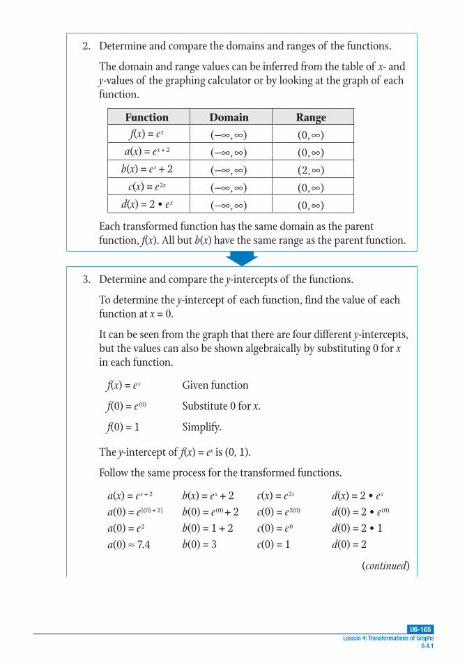
U6-165Lesson 4: Transformations of Graphs
6.4.1
2. Determine and compare the domains and ranges of the functions.
The domain and range values can be inferred from the table of x- and y-values of the graphing calculator or by looking at the graph of each function.
Function Domain Rangef(x) = ex −∞ ∞( , ) ∞(0, )
a(x) = ex + 2 −∞ ∞( , ) ∞(0, )b(x) = ex + 2 −∞ ∞( , ) ∞(2, )
c(x) = e2x −∞ ∞( , ) ∞(0, )d(x) = 2 • ex −∞ ∞( , ) ∞(0, )
Each transformed function has the same domain as the parent function, f(x). All but b(x) have the same range as the parent function.
3. Determine and compare the y-intercepts of the functions.
To determine the y-intercept of each function, find the value of each function at x = 0.
It can be seen from the graph that there are four different y-intercepts, but the values can also be shown algebraically by substituting 0 for x in each function.
f(x) = ex Given function
f(0) = e (0) Substitute 0 for x.
f(0) = 1 Simplify.
The y-intercept of f(x) = ex is (0, 1).
Follow the same process for the transformed functions.
a(x) = ex + 2 b(x) = ex + 2 c(x) = e2x d(x) = 2 • ex
a(0) = e [(0) + 2] b(0) = e (0) + 2 c(0) = e2(0) d(0) = 2 • e (0)
a(0) = e2 b(0) = 1 + 2 c(0) = e0 d(0) = 2 • 1a(0) ≈ 7.4 b(0) = 3 c(0) = 1 d(0) = 2
(continued)

U6-166Unit 6: Mathematical Modeling6.4.1
For each transformed function, write the y-intercept.
• a(x) = ex + 2: approximately (0, 7.4)
• b(x) = ex + 2: (0, 3)
• c(x) = e2x: (0, 1)
• d(x) = 2 • ex: (0, 2)
The y-intercept of c(x) is the same as that of the parent function, f(x); all the other transformations have been shifted up along the y-axis.
4. Determine and compare the x-intercepts of the functions.
To find the x-intercepts, solve each function for y = 0.
None of the functions exist at y = 0. The function b(x) does not exist for values of y that are less than or equal to 2. It can be seen from the graph that the other functions approach but do not reach y = 0.
5. Determine the value of x at the intersection point of the functions a(x) and b(x).
At their intersection point, a(x) = b(x). Therefore, set the right sides of the equations for a(x) and b(x) equal and solve for x.
= ++e ex x 22 Set a(x) equal to b(x).
− =+e ex x 22 Subtract ex from both sides.
− =e ex ( 1) 22 Rewrite using the Distributive Property.
=−
ee
x2
12Divide both sides by e2 – 1.
=−
x
eln
2
12Solve for x using natural logarithms.
( )= − −x eln2 ln 12 Simplify.
x ≈ –1.16The value of x at the intersection point of the functions a(x) and b(x) is approximately –1.16.

U6-167Lesson 4: Transformations of Graphs
6.4.1
Example 2
The graph shows a parent quadratic function f(x) = x2 and two quadratic functions, g(x) and h(x), derived from it. Use the maximum or minimum point of the quadratic functions to derive their equations, and write the functions in a form that indicates the transformation(s) of the parent function. Then, describe what transformation(s) the parent function underwent to result in each transformed function.
–4 –2 2 4
x
5
4
3
2
1
–1
–2
–3
–4
–5
y
g(x)f(x)
h(x)
0
1. Use the vertex form of a quadratic function, f(x) = a(x – h)2 + k, to determine the equation of the transformed function g(x).
Replace f(x) in the equation of the vertex form with y:
y = a(x – h)2 + k
Recall that the vertex of the graph of the quadratic function is also known as the maximum or minimum point of the function and is represented by the coordinate (h, k). (x, y) represents some point on the graph of the function.
To determine the equation of g(x), first identify the vertex of the graph of g(x).
It can be seen from the graph that the vertex of g(x) is (1, –1).
(continued)

U6-168Unit 6: Mathematical Modeling6.4.1
Next, identify an additional point on the graph of g(x).
It can be seen from the graph that an additional point on the graph of g(x) is (0, 1).
Use the vertex (1, –1) and the additional point (0, 1) to find the value of a in the standard form of the equation.
y = a(x – h)2 + k Standard form of a quadratic equation
(1) = a[(0) – (1)]2 + (–1) Substitute (1, –1) for (h, k) and (0, 1) for (x, y).
1 = a(–1)2 – 1 Simplify.
1 = a – 1 Apply the exponent.
2 = a Add 1 to both sides.
The value of a is 2.
Use the value of a and the coordinate of the vertex to write the equation of the transformed function g(x).
y = a(x – h)2 + k Standard form of a quadratic equation
[g(x)] = (2)[x – (1)]2 + (–1) Let a = 2, y = g(x), and (h, k) be (1, –1).
g(x) = 2(x – 1)2 – 1 Simplify.
The equation of the transformed function g(x) in vertex form is g(x) = 2(x – 1)2 – 1.

U6-169Lesson 4: Transformations of Graphs
6.4.1
2. Use the standard form y = a(x – h)2 + k to determine the equation of the transformed function h(x).
It can be seen from the graph of h(x) that the vertex is (–1, 2) and an additional point is (0, –1).
Use the vertex (–1, 2) and the additional point (0, –1) to find the value of a in the standard form equation.
y = a(x – h)2 + k Standard form of a quadratic equation
(–1) = a[(0) – (–1)]2 + (2) Substitute (–1, 2) for (h, k) and (0, –1) for (x, y).
–1 = a(1)2 + 2 Simplify.
–1 = a + 2 Apply the exponent.
–3 = a Subtract 2 from both sides.
The value of a is –3.
Use the value of a and the coordinate of the vertex to write the equation of the transformed function h(x).
y = a(x – h)2 + k Standard form of a quadratic equation
[h(x)] = (–3)[x + (1)]2 + (2) Let a = –3, y = h(x), and (h, k) be (–1, 2).
h(x) = –3(x + 1)2 + 2 Simplify.
The equation of the transformed function h(x) is h(x) = –3(x + 1)2 + 2.
U6-170Unit 6: Mathematical Modeling6.4.1
3. Describe the transformation(s) of the parent function that resulted in the functions g(x) and h(x).
The transformed functions are g(x) = 2(x – 1)2 – 1 and h(x) = –3(x + 1)2 + 2.
To describe the transformation(s) of the parent function f(x) = x2, start inside the parentheses and work outward.
For g(x):
• 1 was subtracted from x to give x – 1 in place of x.
• Then, 2 was multiplied by the “new” squared term, (x – 1)2.
• Lastly, 1 was subtracted from the new squared term and its new coefficient to give the final result, g(x) = 2(x – 1)2 – 1.
For h(x):
• 1 was added to x to give x + 1 in place of x.
• Then, –3 was multiplied by the “new” squared term, (x + 1)2.
• Finally, 2 was added to the new squared term and its new coefficient to give the final result, h(x) = –3(x + 1)2 + 2.

U6-171Lesson 4: Transformations of Graphs
6.4.1
Example 3
Identify the transformation(s) of the parent function f(x) = log x that result in the function g(x) = 1 + 2 • log (3x + 4). Describe the effect of the transformation(s) on the domain and range of the function g(x). Finally, determine the y-intercept(s) of g(x).
1. Identify the transformation(s) of the parent function.
To determine how the parent function f(x) = log x was transformed, compare it to g(x) = 1 + 2 • log (3x + 4).
• First, note that in g(x), the constant 1 is added to 2 • log (3x + 4). Adding a constant to the function value is the transformation g(x) = f(x) + k.
• Also notice that 2 is multiplied by log (3x + 4). Multiplying the function value by a constant is the transformation g(x) = k • f(x).
• The coefficient 3 is in the argument of the logarithm, log (3x + 4). Multiplying the independent variable by a constant is the transformation g(x) = f(kx).
• Furthermore, note the addition of 4 in the argument of the logarithm, log (3x + 4). Adding a constant to the independent variable in the argument of the logarithm is the transformation g(x) = f(x + k).
Therefore, four transformations—g(x) = f(x) + k, g(x) = k • f(x), g(x) = f(kx), and g(x) = f(x + k)—have been performed on the parent function f(x) = log x.

U6-172Unit 6: Mathematical Modeling6.4.1
2. Compare the domain and range of the parent function to those of the transformed function g(x).
The domain of the parent function is ∞(0, ) .
Since g(x) is a logarithmic function, the domain of g(x) is defined
by the argument of the logarithmic term, 3x + 4. The condition
3x + 4 > 0 or >−x4
3 exists on the argument. Therefore, the domain
of g(x) is − ∞
4
3, .
The range of both functions is ( )−∞ ∞, .
The transformations of f(x) that result in g(x) alter the rate at which the function values change, but not their upper and lower bounds.
3. Calculate the y-intercept of g(x).
The y-intercept of g(x) is defined by the function value g(0). Substitute 0 for x and solve for g(0):
g(x) = 1 + 2 • log (3x + 4)
g(0) = 1 + 2 • log [3(0) + 4]
g(0) = 1 + 2 • log 4
g(0) ≈ 2.2
The y-intercept of g(x) = 1 + 2 • log (3x + 4) is approximately 2.2, or (0, 2.2).

U6-173
PRACTICE
UNIT 6 • MATHEMATICAL MODELINGLesson 4: Transformations of Graphs
Lesson 4: Transformations of Graphs6.4.1
For problems 1–3, use the graph of functions f(x) and g(x) to determine the value of the constant for the given general form of both functions. Then, write the equations of f(x) and g(x) in the given form.
1. general form: a(x + b)
–10 –8 –6 –4 –2 2 4 6 8 10
x
10
8
6
4
2
0
–2
–4
–6
–8
–10
y
g(x)
f(x)
2. general form: ax2
– 10 – 8 – 6 – 4 – 2 2 4 6 8 10
x
10
8
6
4
0
– 2
– 4
– 6
– 8
– 10
y
g(x)
f(x)
Practice 6.4.1: Transformations of Parent Graphs
continued
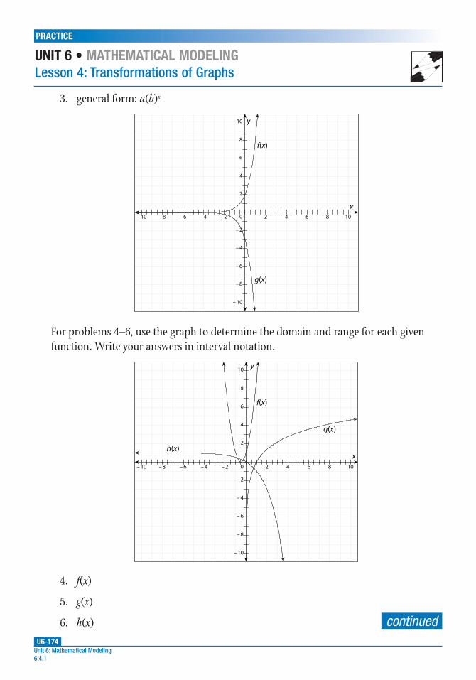
U6-174
PRACTICE
UNIT 6 • MATHEMATICAL MODELINGLesson 4: Transformations of Graphs
Unit 6: Mathematical Modeling6.4.1
3. general form: a(b)x
– 10 – 8 – 6 – 4 – 2 2 4 6 8 10
x
10
8
6
4
2
0
– 2
– 4
– 6
– 8
– 10
y
g(x)
f(x)
For problems 4–6, use the graph to determine the domain and range for each given function. Write your answers in interval notation.
– 10 – 8 – 6 – 4 – 2 2 4 6 8 10
x
10
8
6
4
2
0
– 2
– 4
– 6
– 8
– 10
y
h(x)
g(x)
f(x)
4. f(x)
5. g(x)
6. h(x) continued

U6-175
PRACTICE
UNIT 6 • MATHEMATICAL MODELINGLesson 4: Transformations of Graphs
Lesson 4: Transformations of Graphs6.4.1
Use the information given in each problem to complete problems 7–10.
7. The area of a circle is given by the function A(a, b) = π(a – b)2. What happens to the value of A(a, b) if the value of a is doubled and b is increased by 2?
8. The volume of water flowing into a reservoir is given by the function
V(r, t) = r • t, in which r is the rate in gallons per second and t is the time in
hours. What happens to the value of t if the volume is doubled and r is
decreased by a factor of 2
3?
9. The pH of a polluted stream is given by the function p(c) = –log c, in which c is the concentration of acid ions in the stream. The range of p is (0, 14) since the pH scale runs from 0 to 14. How does the domain of c change if the range of p changes to (7, 10)? Recall that on the pH scale, an acidic solution has a pH greater than 7, whereas a basic solution has a pH less than 7.
10. The profit p from selling n units of a product is given by the function p(n) = 375n – 25,000. What is the domain of n if the range of p(n) is (0, 5000)? How does the domain of p change if the constant term –25,000 changes to –40,000 and the coefficient of n increases to 400?
U6-176Unit 6: Mathematical Modeling6.4.2
Lesson 6.4.2: Recognizing Odd and Even FunctionsIntroduction
When working with functions, it can be useful to recognize when a specific domain value or its opposite changes a function value in a particular way. For some functions, f(x) = f(–x); that is, evaluating a function for –x results in a function equation that is the same as the original function. Such a function is defined as an even function. An odd function is a function that, when evaluated for –x, results in a function equation that is the opposite of the original function; f(–x) = –f(x). Even and odd functions can be changed into other functions using transformations. In some cases, these changed functions are still even or odd functions, but in other cases they no longer meet the criteria for being even or odd.
Key Concepts
• A function f(x) for which f(x) = f(–x) is defined as an even function.
• A function f(x) for which f(x) = –f(–x) is defined as an odd function.
• Whether a function is even, odd, or neither can be determined algebraically by substituting –x for x and comparing the result to the original function.
• The transformations g(x) = f(kx), g(x) = k • f(x), and g(x) = f(x + k) of an even function result in an even function.
• The transformation g(x) = f(x) + k of an even function results in an even function.
• The transformation g(x) = f(x) + k of an odd function results in a new function that is neither even nor odd.
• A function that contains terms with both odd and even exponents is neither an even nor an odd function.
• To quickly determine if a function is even, odd, or neither, look at its graph:
• The graph of an even function is symmetric about the y-axis.
• The graph of an odd function is symmetric about the origin.
• The graph of a function that is neither odd nor even is not symmetric about either the y-axis or the origin.
• The graphs of trigonometric functions can also be described as even or odd. For example, sine functions are odd, whereas cosine functions are even.
• A graphing calculator can be especially useful for evaluating evenness or oddness for higher-degree polynomials or other non-polynomial functions.
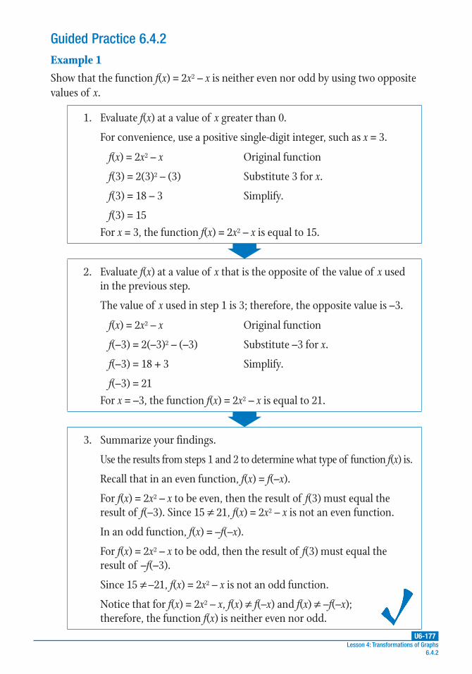
U6-177Lesson 4: Transformations of Graphs
6.4.2
Guided Practice 6.4.2Example 1
Show that the function f(x) = 2x2 – x is neither even nor odd by using two opposite values of x.
1. Evaluate f(x) at a value of x greater than 0.
For convenience, use a positive single-digit integer, such as x = 3.
f(x) = 2x2 – x Original function
f(3) = 2(3)2 – (3) Substitute 3 for x.
f(3) = 18 – 3 Simplify.
f(3) = 15For x = 3, the function f(x) = 2x2 – x is equal to 15.
2. Evaluate f(x) at a value of x that is the opposite of the value of x used in the previous step.
The value of x used in step 1 is 3; therefore, the opposite value is –3.
f(x) = 2x2 – x Original function
f(–3) = 2(–3)2 – (–3) Substitute –3 for x.
f(–3) = 18 + 3 Simplify.
f(–3) = 21For x = –3, the function f(x) = 2x2 – x is equal to 21.
3. Summarize your findings.
Use the results from steps 1 and 2 to determine what type of function f(x) is.
Recall that in an even function, f(x) = f(–x).
For f(x) = 2x2 – x to be even, then the result of f(3) must equal the result of f(–3). Since 15 ≠ 21, f(x) = 2x2 – x is not an even function.
In an odd function, f(x) = –f(–x).
For f(x) = 2x2 – x to be odd, then the result of f(3) must equal the result of –f(–3).
Since 15 ≠ –21, f(x) = 2x2 – x is not an odd function.
Notice that for f(x) = 2x2 – x, f(x) ≠ f(–x) and f(x) ≠ –f(–x); therefore, the function f(x) is neither even nor odd.

U6-178Unit 6: Mathematical Modeling6.4.2
Example 2
Describe how the graph of the function g(x) = x3 – 2x can be used to determine if the function is even or odd.
1. Graph the function by hand or using a graphing calculator.
The graph of g(x) = x3 – 2x is as follows.
–10 –8 –6 –4 –2 2 4 6 8 10
x
10
8
6
4
2
0
–2
–4
–6
–8
–10
y
g(x) = x3 – 2x
2. Visually compare the parts of the graph to the right and left of the y-axis.
From the graph, it can be seen that graph is symmetric about the origin.
Notice that when x = 1, y = –1, or (1, –1).
Also notice that when x = –1, y = 1, or (–1, 1).
Therefore, it can be hypothesized that opposite values of x result in opposite values of y.
3. Summarize your findings.
The function g(x) is an odd function since it can be seen from the graph that g(x) = –g(–x).
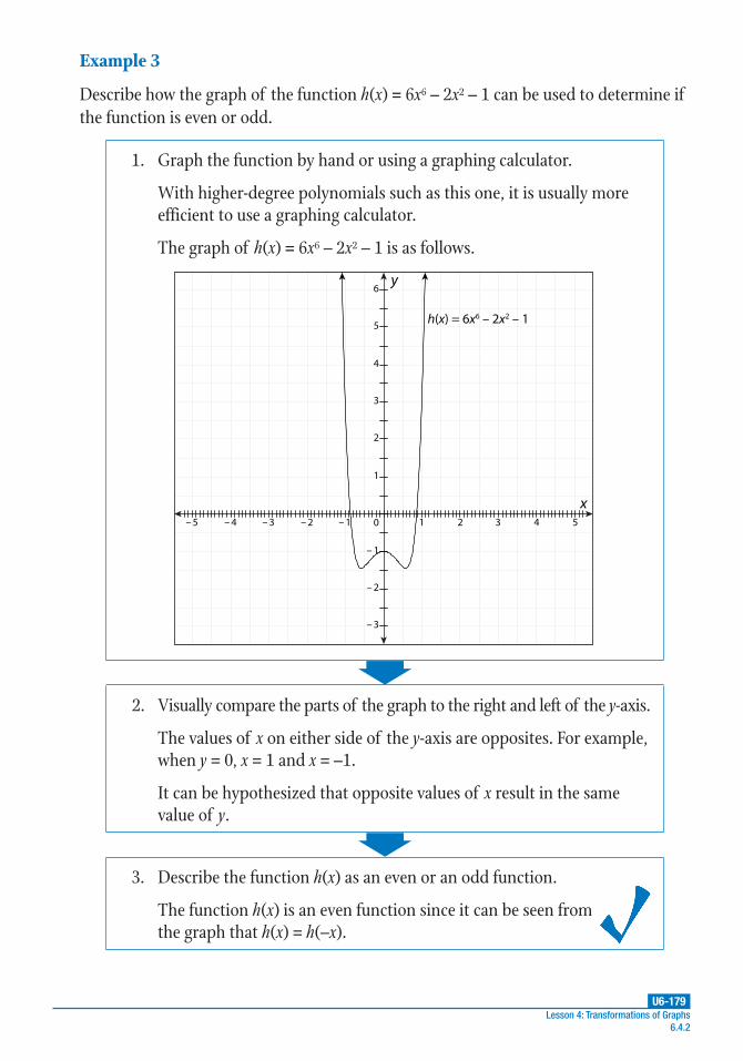
U6-179Lesson 4: Transformations of Graphs
6.4.2
Example 3
Describe how the graph of the function h(x) = 6x6 – 2x2 – 1 can be used to determine if the function is even or odd.
1. Graph the function by hand or using a graphing calculator.
With higher-degree polynomials such as this one, it is usually more efficient to use a graphing calculator.
The graph of h(x) = 6x6 – 2x2 – 1 is as follows.
– 5 – 4 – 3 – 2 – 1 1 2 3 4 5
x
6
5
4
3
2
1
0
– 1
– 2
– 3
y
h(x) = 6x6 – 2x2 – 1
2. Visually compare the parts of the graph to the right and left of the y-axis.
The values of x on either side of the y-axis are opposites. For example, when y = 0, x = 1 and x = –1.
It can be hypothesized that opposite values of x result in the same value of y.
3. Describe the function h(x) as an even or an odd function.
The function h(x) is an even function since it can be seen from the graph that h(x) = h(–x).

U6-180Unit 6: Mathematical Modeling6.4.2
Example 4
Compare the functions f(x) = log x2 and g(x) = 2 • log x using the definitions of even and odd functions.
1. Determine the domain values for which f(x) exists.
The domain of f(x) is ( )−∞ ∩ ∞,0) (0, since the argument of the logarithm squares the value of x.
2. Describe f(x) using the definitions of even and odd functions.
The function f(x) = log x2 can be described as an even function since it can be written as f(x) = f(–x) = log x2. (Recall that the square of a negative term is positive.)
3. Determine the domain values for which g(x) exists.
g(x) is a logarithmic function; therefore, the domain of g(x) is ( )∞0, .
4. Describe g(x) using the definitions of even and odd functions.
Notice that the function f(x) = log x2 can be written as f(x) = 2 • log x, which is the same as g(x) = 2 • log x.
The function f(x) = 2 • log x is neither even nor odd since f(x) ≠ f(–x) ≠ –f(–x); therefore, g(x) is also neither even nor odd.
5. Summarize your findings.
The function f(x) = log x2 is an even function, but its rewritten form, g(x), is not.
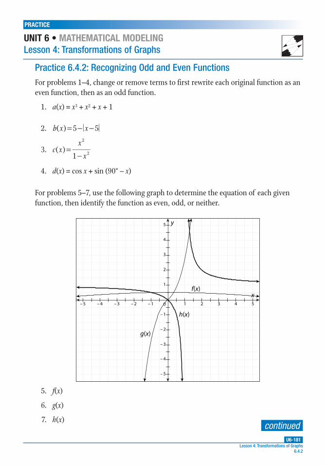
U6-181
PRACTICE
UNIT 6 • MATHEMATICAL MODELINGLesson 4: Transformations of Graphs
Lesson 4: Transformations of Graphs6.4.2
For problems 1–4, change or remove terms to first rewrite each original function as an even function, then as an odd function.
1. a(x) = x3 + x2 + x + 1
2. = − −b x x( ) 5 5
3. =−
c xx
x( )
1
2
2
4. d(x) = cos x + sin (90° – x)
For problems 5–7, use the following graph to determine the equation of each given function, then identify the function as even, odd, or neither.
– 5 – 4 – 3 – 2 – 1 1 2 3 4 5
x
5
4
3
2
1
0
– 1
– 2
– 3
– 4
– 5
y
h(x)
g(x)
f(x)
5. f(x)
6. g(x)
7. h(x)
Practice 6.4.2: Recognizing Odd and Even Functions
continued

U6-182
PRACTICE
UNIT 6 • MATHEMATICAL MODELINGLesson 4: Transformations of Graphs
Unit 6: Mathematical Modeling6.4.2
Use the information and the graph that follows to complete problems 8–10.
Most spiders have 8 eyes—2 “primary” eyes that detect images, and 6 “secondary” eyes that detect shadows and the difference between light and dark. The two types work together to detect the average intensity of light. A primary eye can see polarized light, which is phase shifted from what a secondary eye sees. Mathematically, the light seen by each type of eye can be represented by the functions I1(t) = Imax • (1 + cos t) and I2(t) = Imax • (1 – cos t), in which Imax is the maximum intensity of each oscillating light wave, and each cosine term represents the varying intensity of the light with time. The graph shows the two cosine terms, I1(t) and I2(t), and the average intensity function, I(t).
–5 –4 –3 –2 –1 1 2 3 4 5
I(t)
5
4
3
2
1
0
–1
–2
–3
–4
–5
I
t
I2(t)I
1(t)
8. Are the functions I1(t) and I2(t) even, odd, or neither?
9. Write a function for the average intensity of the light waves. (Hint: Recall the definition of an arithmetic mean or “average” of two numbers.)
10. Suppose one light wave is represented as f(x) = cos x and the other is represented by g(x) = cos (90° – x). Use the definitions of even and odd functions to determine if f(x) and g(x) are even or odd functions.

Lesson 5: Comparing Properties Within and Between Functions
UNIT 6 • MATHEMATICAL MODELING
U6-183Lesson 5: Comparing Properties Within and Between Functions
6.5
Essential Questions
1. What is the significance of a difference in x- or y-intercepts of different forms of the same function or in comparing two or more functions in real-world situations?
2. In a real-world problem, how does a function model change when different domains result in positive and negative values?
3. When are maximum and minimum function values relevant to solving or visualizing real-world problems?
4. What are the limitations on the domain of a real-world function and how do these limitations affect function values and possible solutions to real-world problems?
5. How do variations in the rate of change of a function value affect the interpretation of real-world problems in which rate of change is a factor?
Common Core Georgia Performance Standards
MCC9–12.F.IF.4★
MCC9–12.F.IF.5★
MCC9–12.F.IF.6★
MCC9–12.F.IF.9
WORDS TO KNOW
asymptote an equation that represents sets of points that are not allowed by the conditions in a parent function or model; a line that a function gets closer and closer to, but never crosses or touches
average rate of change the ratio of the difference of output values to
the difference of the corresponding input values: −−
f b f a
b a
( ) ( ); a measure of how a quantity changes over
some interval

U6-184Unit 6: Mathematical Modeling6.5
boundary condition a constraint or limit on a function or domain value based on real-world conditions or restraints in the problem or its solution
delta (D) a Greek letter commonly used to represent the change in a value
extrema the minima or maxima of a function
initial condition a constraint or limit on a function or domain value that exists in the form of a y-intercept or other starting-point mathematical restraint in a real-world problem or solution
local maximum the greatest value of a function for a particular interval of the function; also known as a relative maximum
local minimum the smallest value of a function for a particular interval of the function; also known as a relative minimum
periodic function a function whose values repeat at regular intervals
rate of change a ratio that describes how much one quantity changes with respect to the change in another quantity; also known as the slope of a line
relative maximum the greatest value of a function for a particular interval of the function; also known as a local maximum
relative minimum the smallest value of a function for a particular interval of the function; also known as a local minimum
symmetry of a function the property whereby a function exhibits the same behavior (e.g., graph shape, function values, etc.) for specific domain values and their opposites

U6-185Lesson 5: Comparing Properties Within and Between Functions
6.5
Recommended Resources
• Interactivate. “Data Flyer.”
http://www.walch.com/rr/00243
This applet allows users to create graphs by entering data points, then derive the function equation that fits the graph. Graphs can be manipulated to see how changing the constant and/or coefficient affects the shape of the graph.
• OnlineMathLearning.com. “Compare Two Functions.”
http://www.walch.com/rr/00244
This site offers users access to several videos comparing the properties and features of different types of functions.
• Virtual Nerd. “How Do You Make an Approximate Graph from a Word Problem?”
http://www.walch.com/rr/00245
This video tutorial covers how to sketch the graph of a problem using information derived from a word problem.
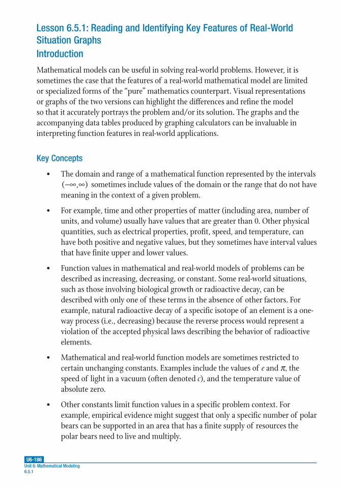
U6-186Unit 6: Mathematical Modeling6.5.1
Introduction
Mathematical models can be useful in solving real-world problems. However, it is sometimes the case that the features of a real-world mathematical model are limited or specialized forms of the “pure” mathematics counterpart. Visual representations or graphs of the two versions can highlight the differences and refine the model so that it accurately portrays the problem and/or its solution. The graphs and the accompanying data tables produced by graphing calculators can be invaluable in interpreting function features in real-world applications.
Key Concepts
• The domain and range of a mathematical function represented by the intervals −∞ ∞( , ) sometimes include values of the domain or the range that do not have
meaning in the context of a given problem.
• For example, time and other properties of matter (including area, number of units, and volume) usually have values that are greater than 0. Other physical quantities, such as electrical properties, profit, speed, and temperature, can have both positive and negative values, but they sometimes have interval values that have finite upper and lower values.
• Function values in mathematical and real-world models of problems can be described as increasing, decreasing, or constant. Some real-world situations, such as those involving biological growth or radioactive decay, can be described with only one of these terms in the absence of other factors. For example, natural radioactive decay of a specific isotope of an element is a one-way process (i.e., decreasing) because the reverse process would represent a violation of the accepted physical laws describing the behavior of radioactive elements.
• Mathematical and real-world function models are sometimes restricted to certain unchanging constants. Examples include the values of e and π, the speed of light in a vacuum (often denoted c), and the temperature value of absolute zero.
• Other constants limit function values in a specific problem context. For example, empirical evidence might suggest that only a specific number of polar bears can be supported in an area that has a finite supply of resources the polar bears need to live and multiply.
Lesson 6.5.1: Reading and Identifying Key Features of Real-World Situation Graphs
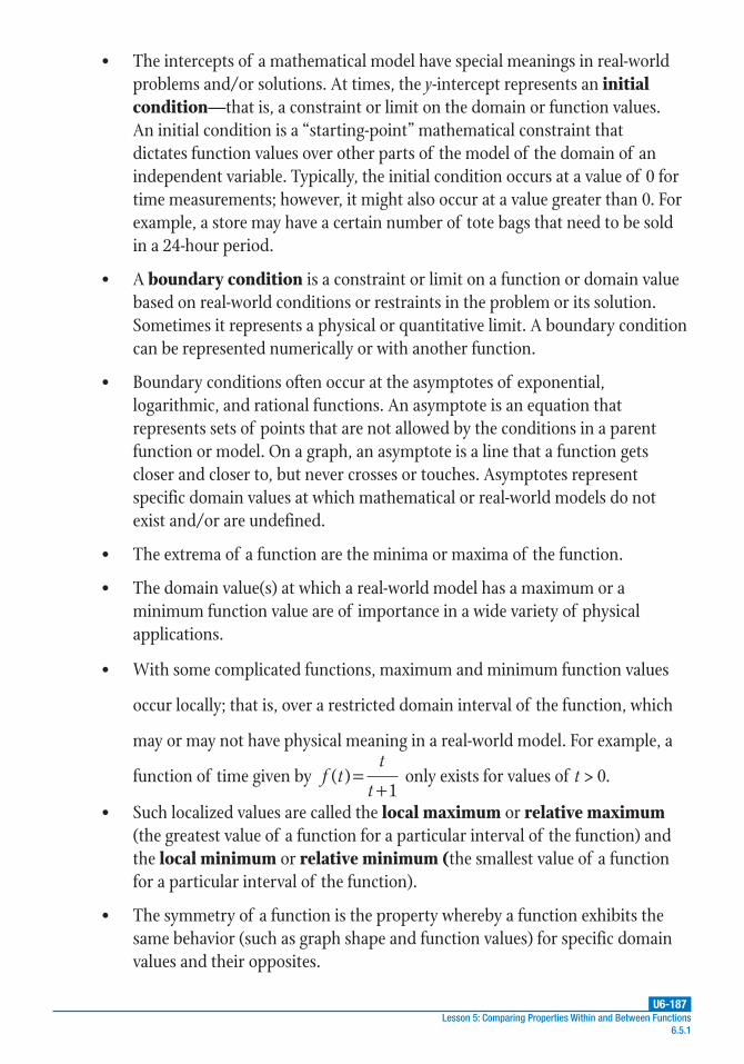
U6-187Lesson 5: Comparing Properties Within and Between Functions
6.5.1
• The intercepts of a mathematical model have special meanings in real-world problems and/or solutions. At times, the y-intercept represents an initial condition—that is, a constraint or limit on the domain or function values. An initial condition is a “starting-point” mathematical constraint that dictates function values over other parts of the model of the domain of an independent variable. Typically, the initial condition occurs at a value of 0 for time measurements; however, it might also occur at a value greater than 0. For example, a store may have a certain number of tote bags that need to be sold in a 24-hour period.
• A boundary condition is a constraint or limit on a function or domain value based on real-world conditions or restraints in the problem or its solution. Sometimes it represents a physical or quantitative limit. A boundary condition can be represented numerically or with another function.
• Boundary conditions often occur at the asymptotes of exponential, logarithmic, and rational functions. An asymptote is an equation that represents sets of points that are not allowed by the conditions in a parent function or model. On a graph, an asymptote is a line that a function gets closer and closer to, but never crosses or touches. Asymptotes represent specific domain values at which mathematical or real-world models do not exist and/or are undefined.
• The extrema of a function are the minima or maxima of the function.
• The domain value(s) at which a real-world model has a maximum or a minimum function value are of importance in a wide variety of physical applications.
• With some complicated functions, maximum and minimum function values
occur locally; that is, over a restricted domain interval of the function, which
may or may not have physical meaning in a real-world model. For example, a
function of time given by =+
f tt
t( )
1 only exists for values of t > 0.
• Such localized values are called the local maximum or relative maximum (the greatest value of a function for a particular interval of the function) and the local minimum or relative minimum (the smallest value of a function for a particular interval of the function).
• The symmetry of a function is the property whereby a function exhibits the same behavior (such as graph shape and function values) for specific domain values and their opposites.

U6-188Unit 6: Mathematical Modeling6.5.1
• Symmetry can be useful in determining if all of the solutions of a model have been identified and if they have relevance for the solution of the real-world context being modeled.
• Symmetries can exist across axes or across lines representing linear equations such as f(x) = x, as is the case with functions and their inverses. A special type of symmetry exists for periodic functions. A periodic function is a function whose values repeat at regular intervals —that is, it exhibits the same function values or properties over repeating restricted domains.
• The behavior of functions for very large and very small domain values can be important in solving real-world problems and describing restrictions on the domain and range values over which a mathematical model can describe a real-world situation.
• For example, compare the functions =+
f tt
t( )
1 and =
+g t
t
t( )
2. For small
values of t such as t = 1, the function values can vary by significant amounts:
f(1) = 0.5 and g =(1) 0.3. For very large values of t, both functions approach
a value of 1; for example, for t = 100, f(100) is about 0.9901, whereas g(100) is
about 0.98. The difference between these two models for “large” values of t is
about 1 percent. On the other hand, for very small values of t, such as t = 0.01,
f(0.01) is about 0.01 whereas g(0.01) is about 0.005; the difference between the
function values for this “small” value of t is about 100 percent.

U6-189Lesson 5: Comparing Properties Within and Between Functions
6.5.1
Example 1
The function for finding the amount of time it takes two workers to complete a job
is given by = +t t t
1 1 1
both 1 2
. Compare this to the function = +1 1 1
2 1 2f d d, which relates
the focal length f2 of a lens to the distances between the lens and an object (d1)
and between the lens and the image of the object created by the lens (d2). F2 and F1
represent the focal points of the two-sided lens. How are the domains and ranges of
these two functions alike and different? Solve each function for the function variable
on the left side of each equation. How do the variable relationships differ?
1. State the restrictions, if any, on the domain and range of the first function, tboth.
None of the variables can equal 0 since they are in the denominators of fractions. The variables measure time, so the values of all three variables are assumed to be greater than 0. Therefore, for tboth, the restricted domain is t1 > 0 and t2 > 0, and the range is tboth > 0.
2. State the restrictions, if any, on the domain and range of the second function, f2.
None of the variables can equal 0 since they are in the denominators of fractions. According to the diagram, the variables can be positive or negative. The location of the image and/or the object being magnified could be “inside” the focal length f2 ; i.e., between the focal point F2 and the origin. Therefore, for f2, the restricted domain is d1 ≠ 0 and d2 ≠ 0, and the range is f2 ≠ 0 .
Guided Practice 6.5.1
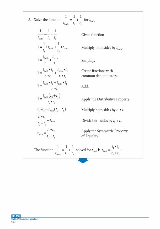
U6-190Unit 6: Mathematical Modeling6.5.1
3. Solve the function = +t t t
1 1 1
both 1 2
for tboth.
= +t t t
1 1 1
both 1 2
Given function
= +t
tt
t11
•1
•1
both2
both Multiply both sides by tboth.
= +t
t
t
t1 both
1
both
2
Simplify.
= +t t
t t
t t
t t1
•
•
•
•both 2
1 2
both 1
2 1
Create fractions with common denominators.
=+t t t t
t t1
• •
•both 2 both 1
1 2
Add.
( )=
+t t t
t t1
•both 2 1
1 2
Apply the Distributive Property.
( )= +t t t t t•1 2 both 2 1 Multiply both sides by t1 • t2.
+=
t t
t tt
•1 2
2 1both Divide both sides by t2 + t1.
=+
tt t
t t
•both
1 2
2 1
Apply the Symmetric Property of Equality.
The function = +t t t
1 1 1
both 1 2
solved for tboth is =+
tt t
t t
•both
1 2
2 1
.
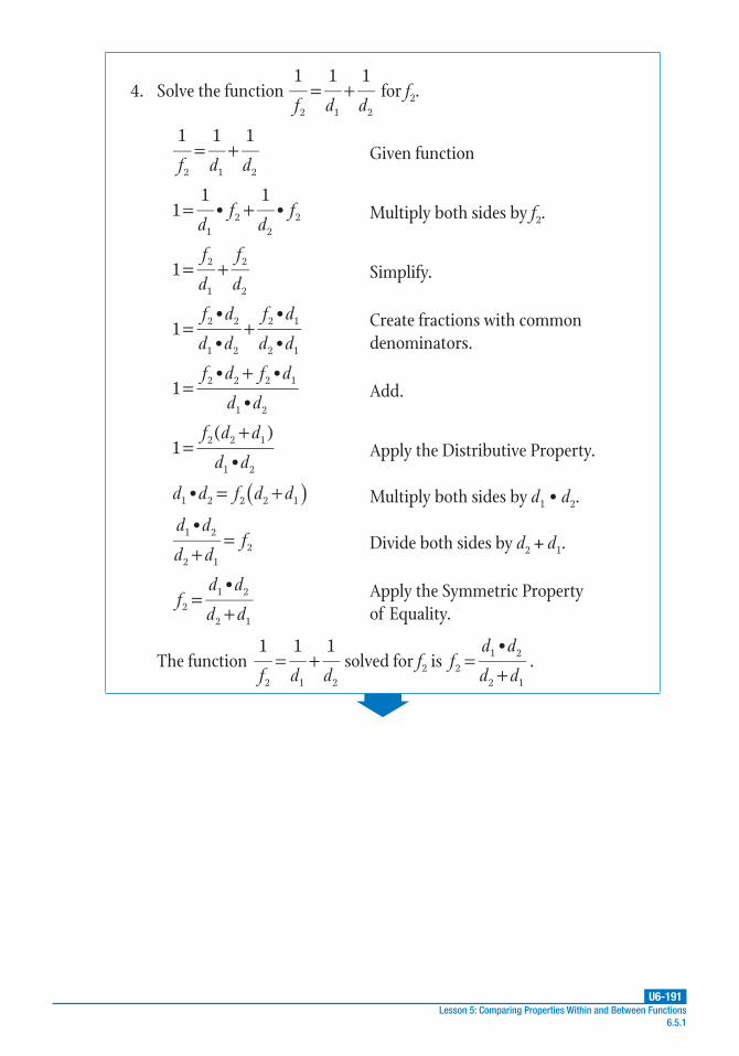
U6-191Lesson 5: Comparing Properties Within and Between Functions
6.5.1
4. Solve the function = +1 1 1
2 1 2f d d for f2.
= +1 1 1
2 1 2f d dGiven function
= +11
•1
•1
22
2df
df Multiply both sides by f2.
= +1 2
1
2
2
f
d
f
dSimplify.
= +1•
•
•
•2 2
1 2
2 1
2 1
f d
d d
f d
d dCreate fractions with common denominators.
=+
1• •
•2 2 2 1
1 2
f d f d
d dAdd.
=+
1( )
•2 2 1
1 2
f d d
d dApply the Distributive Property.
( )= +•1 2 2 2 1d d f d d Multiply both sides by d1 • d2.
+=
•1 2
2 12
d d
d df Divide both sides by d2 + d1.
=+•
21 2
2 1
fd d
d dApply the Symmetric Property of Equality.
The function = +1 1 1
2 1 2f d d solved for f2 is =
+•
21 2
2 1
fd d
d d.

U6-192Unit 6: Mathematical Modeling6.5.1
5. Use the restrictions on the domain and range of each function to compare the relationships between the variables in the functions.
For tboth, the restricted domain is t1 > 0 and t2 > 0, and the range is
tboth > 0. As a result of these restrictions, the variables in =+
tt t
t t
•both
1 2
2 1
are all positive, so the function value will always be positive.
For f2, the restricted domain is d1 ≠ 0 and d2 ≠ 0, and the range is
f2 ≠ 0. As a result of these restrictions, the variables in =+•
21 2
2 1
fd d
d d
could be positive or negative, so f2 could be positive or negative.
Also, the condition d2 + d1 ≠ 0 must be observed in order for the
function f2 to exist.
In summary, the domain and range values for tboth will always be positive. Values of the range of the second function, f2, can be positive or negative, but the function is only valid for domain values that do not sum to 0 (d2 + d1 ≠ 0).

U6-193Lesson 5: Comparing Properties Within and Between Functions
6.5.1
Example 2
Working together, carpenters Benjamin and Ava can build a table in 4 hours. Use the
function =+
tt t
t t
•both
1 2
1 2
to create a graph and to find the time required for each carpenter
to build a table separately if Benjamin takes t hours and Ava takes t + 2 hours.
1. Define the variables in the function.
Using the given information, let t1 = t hours, t2 = t + 2 hours, and tboth = 4 hours.
2. Substitute the defined variables into the given function and simplify.
=+
tt t
t t
•both
1 2
1 2
Given function
( ) ( ) ( )( ) ( )=
++ +
t t
t t4
• 2
2Substitute t for t1, t + 2 for t2, and 4 for tboth.
=+
+ +t t
t t4
2
( 2)
2
Simplify the numerator.
=++
t t
t4
2
2 2
2
Simplify the denominator.
4(2t + 2) = t2 + 2t Multiply both sides by 2t + 2.
8t + 8 = t2 + 2t Distribute.
0 = t2 – 6t – 8 Rewrite the equation so that all terms are on one side.
The simplified function can be written as 0 = t2 – 6t – 8.
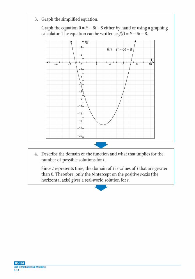
U6-194Unit 6: Mathematical Modeling6.5.1
3. Graph the simplified equation.
Graph the equation 0 = t2 – 6t – 8 either by hand or using a graphing calculator. The equation can be written as f(t) = t2 – 6t – 8.
–4 –2 2 4 6 8 10
t
4
2
0
–2
–4
–6
–8
–10
–12
–14
–16
–18
–20
f(t)
f(t) = t2 – 6t – 8
4. Describe the domain of the function and what that implies for the number of possible solutions for t.
Since t represents time, the domain of t is values of t that are greater than 0. Therefore, only the t-intercept on the positive t-axis (the horizontal axis) gives a real-world solution for t.
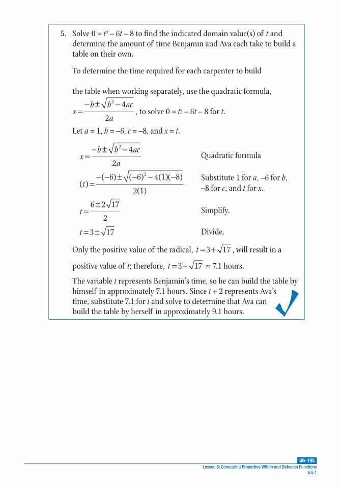
U6-195Lesson 5: Comparing Properties Within and Between Functions
6.5.1
5. Solve 0 = t2 – 6t – 8 to find the indicated domain value(s) of t and determine the amount of time Benjamin and Ava each take to build a table on their own.
To determine the time required for each carpenter to build
the table when working separately, use the quadratic formula,
=− ± −
xb b ac
a
4
2
2
, to solve 0 = t2 – 6t – 8 for t.
Let a = 1, b = –6, c = –8, and x = t.
=− ± −
xb b ac
a
4
2
2
Quadratic formula
=− − ± − − −
t( )( 6) ( 6) 4(1)( 8)
2(1)
2 Substitute 1 for a, –6 for b, –8 for c, and t for x.
=±
t6 2 17
2Simplify.
= ±t 3 17 Divide.
Only the positive value of the radical, = +t 3 17 , will result in a
positive value of t; therefore, = +t 3 17 ≈ 7.1 hours.
The variable t represents Benjamin’s time, so he can build the table by himself in approximately 7.1 hours. Since t + 2 represents Ava’s time, substitute 7.1 for t and solve to determine that Ava can build the table by herself in approximately 9.1 hours.

U6-196Unit 6: Mathematical Modeling6.5.1
Example 3
The diagram shows the distance (d1) between an object and a lens and the distance (d2)
between the lens and the image it creates of the object. F1 and F2 represent the focal
points of the two-sided lens. (Note that these points are symmetric about the lens
at line l.) Use the diagram and the function =+•
11 2
1 2
fd d
d d to find d1 and d2 if the focal
length f1 of the lens is –1 and d2 = –d1 + 2.
f1
f2
F1
F2
d1
d2
0
Object
Image
Lensl
1. Define the variables in the function.
Using the given information, let f1 = –1 and d2 = –d1 + 2.
2. Substitute the defined variables into the given function and simplify.
Substitute each of the defined variables into the given function.
=+•
11 2
1 2
fd d
d d Given function
( 1)•( 2)
( 2)1 1
1 1
− =− +
+ − +d d
d dSubstitute –1 for f1 and –d1 + 2 for d2.
12•
( 2)1
21
1 1
( )− =
− ++ − +d d
d dDistribute the numerator.
12•
21
21( )
− =− +d d
Simplify the denominator.
–2 = –(d1)2 + 2 • d1 Multiply both sides by 2.
0 = (d1)2 – 2 • d1 – 2 Set all terms on one side with a positive leading coefficient.
The simplified function can be written as 0 = (d1)2 – 2d1 – 2.

U6-197Lesson 5: Comparing Properties Within and Between Functions
6.5.1
3. Graphthesimplifiedequation.
Graphtheequation0=(d1)2–2d1 –2byhandorusingagraphingcalculator.Thisequationcanbewrittenasf(d1)=(d1)2–2d1 –2.
– 10 – 8 – 6 – 4 – 2 2 4 6 8 10
x
10
8
6
4
2
0
– 2
– 4
– 6
– 8
– 10
y
f(d1) = (d1)2 – 2d1 – 2
4. Describethedomainof thefunctionandwhatthatimpliesforthenumberof possiblesolutionsford1andd2.
Thevariablescannotequal0,buttheycanbepositiveornegative.Thelensdiagramshowsthatd1andd2canbepositiveornegative,dependingonwheretheobjectislocatedrelativetothelens.
TheobjectcouldbelocatedbetweenthefocalpointF2andthelensoranywheretotheleftof thefocalpointF2,asshowninthediagram.Thiscreatesthepossibilityof aninfinitenumberof possiblesolutionsford1andd2.

U6-198Unit 6: Mathematical Modeling6.5.1
5. Solve 0 = (d1)2 – 2d1 – 2 to find the value(s) of d1 as described in step 4.
To solve 0 = (d1)2 – 2d1 – 2, use the quadratic formula,
=− ± −
xb b ac
a
4
2
2
.
Let a = 1, b = –2, c = –2, and x = d1.
=− ± −
xb b ac
a
4
2
2
Quadratic formula
d( 2) (–2) 4(1)(–2)
2(1)1
2
( )=− − ± − Substitute 1 for a, –2 for b,
–2 for c, and d1 for x.
112
21 = ±d Simplify.
d 1 31 = ±
The solutions are 1 3 2.731 = + ≈d or 1 3 0.731 = − ≈−d .
6. Find d2 and interpret the solutions in terms of the locations of the object and image in relation to the lens.
The two distances are related by the formula d2 = –d1 + 2. Since d1 ≈ 2.73 or –0.73, substitute each of these values into the formula and solve for d2.
d2 = –d1 + 2 d2 = –d1 + 2
d2 ≈ –(2.73) + 2 d2 ≈ –(–0.73) + 2
d2 ≈ –0.73 d2 ≈ 2.73
The focal length, f1, was given as –1, which means it is measured to
the left of the lens.
A negative value for d2 means the image is on the left side of the lens. A positive value for d2 means the image is on the right side of the lens.

U6-199Lesson 5: Comparing Properties Within and Between Functions
6.5.1
Example 4
The table shows the number of earthquakes of six different average magnitudes detected over the course of a year by the Earthquake Hazards Program of the U.S. Geological Survey.
Magnitude, m 6.0 6.5 7.0 7.5 8.0 8.5Number, N 210 56 15 3 1 0
Use a graphing calculator to find a natural logarithm function that fits this data. Then choose the scales for a graph of the data based on real-world factors. (Note: The earthquake magnitude is the power of an exponent, which can be positive, negative, or 0.) Describe the shape of the resulting graph.
1. Identify the dependent and independent variables.
The number of earthquakes N depends on the magnitude m, so N is the dependent variable and m is the independent variable.
2. Use these variables to write the general form of the natural logarithm function.
The parent function of the natural logarithm function is f(x) = ln x, so this function will be of the form N(m) = ln m.
3. Use a graphing calculator to generate a natural logarithm function from the table data.
You will need to refer to the resulting table of values later, so keep your work on the calculator screen.
On a TI-83/84:
Step 1: Press [2ND][Y=] to bring up the STAT PLOTS menu.
Step 2: The first option, Plot 1, will already be highlighted. Press [ENTER].
Step 3: Under Plot 1, select ON if it isn’t selected already.
(continued)
U6-200Unit 6: Mathematical Modeling6.5.1
Step 4: Press [STAT]. Select 1: Edit… to open a table. Arrow up to L1, then press [CLEAR][ENTER] to clear the list. Repeat as needed. Press [ENTER].
Step 5: From L1, press the down arrow to move your cursor into the list. Enter the values from the table for each magnitude, pressing [ENTER] after each number to navigate to the next blank spot in the list.
Step 6: Arrow over to the L2 column. Enter the corresponding values representing the number of earthquakes for each magnitude.
Step 7: To fit an equation to the data points, press [STAT] and arrow over to the CALC menu. Then, select 9: LnReg, “natural logarithm regression.”
Step 8: Press [2ND][1] to type “L1” for Xlist. Press [,], then arrow down to Ylist and press [2ND][2] to type “L2” for Ylist, if not already shown.
Step 9: Arrow down to “Calculate” and press [ENTER] to generate a natural logarithm function of the form y = a + b • ln x.
On a TI-Nspire:
Step 1: Press [home]. Arrow over to the spreadsheet icon, the fourth icon from the left, and press [enter].
Step 2: To clear the lists in your calculator, arrow up to the topmost cell of the table to highlight the entire column, then press [menu]. Choose 3: Data, then 4: Clear Data. Repeat for each column as necessary.
Step 3: Arrow over to column A. Name the column “m” and enter the values from the table for each magnitude, pressing [enter] to navigate to the next blank cell.
Step 4: Arrow over to column B. Name the column “n” and enter the corresponding values representing the number of earthquakes for each magnitude.
(continued)

U6-201Lesson 5: Comparing Properties Within and Between Functions
6.5.1
Step 5: To generate a natural logarithm function with the data, press [menu]. Select 4: Statistics, then 1: Stat Calculations, and then B: Logarithmic Regression…. Press [enter].
Step 6: Use the pop-up menus to enter “m” in the X List field and “n” in the Y List field. Tab to OK and press [enter]. This will generate a natural logarithm function of the form y = a + b • ln x. The coefficients appear on the right side of the screen in column D.
Either calculator will return approximate results of a ≈ 1075.78 and b ≈ –520.92.
4. Write the function and enter it on the graphing calculator.
To write a natural logarithm function of the form y = a + b • ln x, let y = N(m), a = 1075.78, b = –520.92, and x = m.
The function that approximately fits the table data is N(m) = 1075.78 – 520.92 • ln m.
Enter the function on the graphing calculator.
5. Select a scale for the dependent and independent variable axes on a graph of the data.
The m values range from 6.0 to 8.5, so an independent variable scale could be from m = 0 to m = 10. The N values range from 0 to 210, so a dependent variable scale could be from N = 0 to N = 250 with a scale of 25 for each interval on the axis. Other scales are acceptable as long as they show all of the data points in the table.
6. Use the results to adjust the scales of the graphing calculator’s viewing window, then graph the natural logarithm function and table data.
On a TI-83/84:
Step 1: Press [WINDOW] and change the x and y scales to the values identified earlier: Xmin = 0, Xmax = 10, Xscl = 1, Ymin = 0, Ymax = 250, and Yscl = 25.
Step 2: Press [GRAPH] to view the data plot and function.(continued)

U6-202Unit 6: Mathematical Modeling6.5.1
On a TI-Nspire:
Step 1: Press [home]. Arrow over to the graphing icon, the second icon from the left, and press [enter].
Step 2: Press [menu], then select 4: Window/Zoom, and then 1: Window Settings. Change the settings as identified earlier: XMin = 5, XMax = 10, XScale = Auto, YMin = 0, YMax = 250, and YScale = 25. Tab to “OK” and press [enter] to save the settings.
Step 3: Press [menu] when the new window appears and select 3: Graph Type and 4: Scatter Plot.
Step 4: At the bottom of the graph window, beside x type m. Press [tab].
Step 5: Beside y, type n. Press [enter]. The points will appear on the graph.
The result on either calculator includes the data points and the natural logarithm function. (Note: Save this data for use with Example 5.)
2 4 6 8 10
m
240
220
200
180
160
140
120
100
80
60
40
20
0
N(m)
N(m) = 1075.78 – 520.92 • ln m

U6-203Lesson 5: Comparing Properties Within and Between Functions
6.5.1
7. Describe the shape of the graph in terms of how the function values change as the earthquake magnitude increases from 6.0 to 8.5 and in terms of changes in N as m changes.
The function value decreases from m = 6.0 to m = 8.5, and the rate of increase also decreases from m = 6.0 to m = 8.5.
The value of N decreases with each step in the value of m(0.5), but the amount of decrease is constant over each interval. For example, N decreases from 210 to 56 for m from 6.0 to 6.5, and N decreases from 56 to 15 for m from 6.5 to 7.
Example 5
Modify the earthquake data from Example 4 (repeated below) by adding a second dependent variable in the graphing calculator table for the natural logarithm of the number of earthquakes—ln N—of each value of m. Graph this new variable and the earthquake magnitude m and describe the resulting graph. Suggest an explanation for the shape and domain of the new graph given that the earthquake magnitude m is defined as the power of an exponent. What restrictions exist on m?
Magnitude, m 6.0 6.5 7.0 7.5 8.0 8.5Number, N 210 56 15 3 1 0
1. Modify the graphing calculator data from Example 4 to add values for ln N of each value of m.
On your graphing calculator, return to the table of values for m and N that you created in Example 4. (If you need to enter the values again, refer to the calculator directions in that example.)
On a TI-83/84:
Note: Recall that L1 represents the independent variable m and L2 represents the dependent variable N; therefore, L3 will represent the third variable, ln N.
Step 1: Press [2ND][Y=] to bring up the STAT PLOTS menu.
Step 2: Select 1: Plot 1..., then arrow down to Data List and press [2ND][3] to change the variable to L3. Press [ENTER] to save the change.
(continued)

U6-204Unit 6: Mathematical Modeling6.5.1
Step 3: Press [STAT]. Select 1: Edit... and press [ENTER].
Step 4: The first N value from column L2 is cell L2(1). To enter the natural logarithm of this value, arrow to the first blank cell in L3. Press [LN][2ND][2][(][1][)]. Press [ENTER].
Step 5: Repeat Step 4 for the other nonzero numbers in the L2 column, following the pattern [LN][2ND][2] and changing the number in parentheses depending on the row.
Step 6: Delete the data from cells L1(6) and L2(6) by pressing [DEL] in each of those cells so the calculator can produce the graph for the variables L1 and L3.
On a TI-Nspire:
Step 1: Press [ctrl] and then press up on the NavPad to view all open documents. Select the table document from Example 4.
Step 2: Navigate to the first cell in column C and press up on the NavPad to highlight the column. Press [clear] to delete the data. Repeat for column D.
Step 3: Highlight the top cell in column C. Use your keypad to enter a name for the natural logarithm of N, such as “lnn.” (Note: The “ln” operation key cannot be used for this since it is a variable name.)
Step 4: The first N value from column B is cell B1. To enter the natural logarithm of this value, arrow to the first blank cell in column C. Press [=][ctrl][ex][B][1]. Press [enter].
Step 5: Repeat Step 4 for the other nonzero numbers in the B column, following the pattern [=][ctrl][ex][B] and changing the last number depending on the row. Do not repeat for the last cell, B6, because the logarithm of 0 is undefined.
Step 6: Clear the data from cells A6 and B6 so the calculator can calculate the graph for the m and “lnn” variables.

U6-205Lesson 5: Comparing Properties Within and Between Functions
6.5.1
2. Select a scale for the dependent and independent variable axes on a graph of the revised data.
The settings for the independent variable m can be the same as those used in Example 4, since those did not change. However, the values of the dependent variable “lnn” vary between 0 and 5.3471, so this scale should be reset to values from –1 to 6. Other scales are acceptable as long as they show all of the data points.
On a TI-83/84:
Step 1: Press [WINDOW] and change the x and y scales as needed to reflect the modified values: Xmin = –1, Xmax = 10, Xscl = 1, Ymin = –1, Ymax = 6, and Yscl = 1.
Step 2: Press [GRAPH] to view the data plot.
On a TI-Nspire:
Step 1: Press [home]. Arrow over to the graphing icon, the second icon from the left, and press [enter].
Step 2: Press [menu], then select 4: Window/Zoom, and then 1: Window Settings. Change the settings as needed to reflect the modified values: XMin = –1, XMax = 10, XScale = Auto, YMin = –1, YMax = 6, and YScale = Auto. Tab to “OK” and press [enter] to save the settings.
Step 3: Press [menu] when the new window appears and select 3: Graph Type and 4: Scatter Plot.
Step 4: At the bottom of the graph window, beside x type m. Press [tab].
Step 5: Beside y, type lnn. Press [enter]. The points will appear on the graph.
(continued)

U6-206Unit 6: Mathematical Modeling6.5.1
The resulting graph is as follows.
10 2 3 4 5 6 7 8 9 10
x
6
5.5
5
4.5
4
3.5
3
2.5
2
1.5
1
0.5
y
3. Describe the shape of the graph.
The graph is a straight line with a negative slope.
4. Suggest an explanation for the shape and domain of the new graph based on the definition of m from the problem statement.
The variable m is described as “the power of an exponent,” which is also a definition of a logarithm. This means that in this graph, one logarithm is plotted against another logarithm plus a constant. The average rate of change of one logarithm relative to the other logarithm is constant in this case, which results in a straight line.
Mathematically, since ln N is undefined for m = 8.5, the domain of the quake magnitudes is restricted to values of m that are less than 8.5. However, since this is a logarithm, recall that the independent variable m will not be less than or equal to 0, as evidenced by the point (8.5, 0). So, since for this real-world situation ln N cannot be less than 0, the domain of the quake magnitudes is restricted to values of m that are less than or equal to 8.5.

U6-207
PRACTICE
UNIT 6 • MATHEMATICAL MODELINGLesson 5: Comparing Properties Within and Between Functions
Lesson 5: Comparing Properties Within and Between Functions6.5.1
The following graph shows the time it takes for three different models of microcircuit lithography-fabricator robots to complete the 10 steps in the production of a tablet computer CPU. The functions f(t), g(t), and h(t) model the productivity of the three robots as they produce a finished and ready-to-test CPU for the next stage of the tablet computer assembly. Use the graph to complete problems 1–3.
1 2 3 4 5 6 7 8 9 10
x
10
9
8
7
6
5
4
3
2
1
0
y
f(t)g(t)
h(t)
Hours
Step
s
1. Describe the behavior of the function model for each of the three robots as they complete the 10 steps over the time interval shown.
2. What is the significance of the point of intersection of the graphs of the three models?
3. Compare the time at which the three robots complete the 10 steps in the real-world of manufacturing and compare that time to the time at which each of the mathematical models indicate that the 10 steps are completed.
Practice 6.5.1: Reading and Identifying Key Features of Real-World Situation Graphs
continued

U6-208
PRACTICE
UNIT 6 • MATHEMATICAL MODELINGLesson 5: Comparing Properties Within and Between Functions
Unit 6: Mathematical Modeling6.5.1
The following graph shows data points representing the increase in the yield of corn Y(t) from 1950 through 2010 in metric tons per hectare (10,000 square meters). The curved line represents a function model of the varying amounts of nitrogen applied to those crops in kilograms per hectare for that time period, which is given by N(t) = 180(1 – 2–t). The year 1950 corresponds to x = 1, the year 1960 to x = 2, and so on. The two different dependent variables are shown on the same graph by using a different y-axis scale for each when analysis or calculations are done. Use the graph to complete problems 4–6.
1 2 3 4 5 6 7 8 9 10
t
18
17
16
15
14
13
12
11
10
9
8
7
6
5
4
3
2
1
180
170
160
150
140
130
120
110
100
90
80
70
60
50
40
30
20
10
0
Y(t)N(t)
4. The y-axis scale for the corn production runs from 0 to 18. Describe a function model or combination of models for the corn-production data points.
5. Determine an appropriate y-axis scale for the amount of nitrogen applied per hectare. Describe how the amount of nitrogen applied changes over the time period from 1950 to 2010.
6. Compare the function you picked for the rate of corn production with the given function model for the rate of application of nitrogen to the crops over the period from 1950 to 2010. Compare and contrast the behavior of each function.
continued

U6-209
PRACTICE
UNIT 6 • MATHEMATICAL MODELINGLesson 5: Comparing Properties Within and Between Functions
Lesson 5: Comparing Properties Within and Between Functions6.5.1
The following graph shows two sine-function models for the growth in numbers of hybrid-electric cars, H(t), and battery-electric cars, B(t), from 2007 and projected out to 2020, for which t is the time in years. The year 2007 corresponds to x = 1, the year 2008 to x = 2, and so on. The y-axis is the historical and projected market share of the two types of vehicles from 0 percent to 6 percent. Use the graph to complete problems 7–10.
20 4 6 8 10 12
t
6
5.5
5
4.5
4
3.5
3
2.5
2
1.5
1
0.5
y
H(t)
B(t)
7. Determine the restricted domain of the function H(t) = 3.2 + 2.2 sin (0.25 • t – 1.5) and its range over that domain.
8. What does the function value H(0) describe?
9. Determine the range of the function B(t) = 1 + sin (0.2 • t – 1.5) over the restricted domain of H(t).
10. Predict which type of vehicle will have the greater rate of market-share increase based on these models. Explain your answer in terms of the period of the two sine-function models.

U6-210Unit 6: Mathematical Modeling6.5.2
Introduction
The rate of change is a ratio that describes how much one quantity changes with respect to the change in another quantity. For a function, the rate of change is the amount by which function values change for each change in domain values. When the rate of change of a function increases by the same amount for every consecutive domain value, the rate of change is said to be constant. Linear functions exhibit this trait; however, not all functions have a constant rate of change.
Key Concepts
• The rate of change of a single function is dependent on the change that occurs between two points (ordered pairs) on the graph of that function. Recall that this is the same as the slope when the function is a line.
• The rate of change of a function is the difference between the values of the
function at two different domain values; mathematically, this can be represented
by the formula �
�
( ) ( ) ( ) ( ) ( )1 2
1 2
2 1
2 1
=−−
=−−
=rf x f x
x x
f x f x
x x
f x
x, in which f1(x) is
the function value at the domain value x1 and f2(x) is the function value at the
domain value x2.
• The uppercase Greek letter delta (D) is commonly used to represent the “change” in a value; for example, Df(x) can be read as “change in f of x.” Therefore, Df(x) and Dx are more concise ways of representing the numerator and denominator, respectively, in the rate of change formula.
• Note that the order in which the function values are compared must be the same as the order in which the domain values are compared. Mixing up the order of the values in the numerator with the order of the values in the denominator will result in an incorrect rate calculation.
• The average rate of change is the average of all of the different rates of
change of a function value over a restricted domain. Formally, it is the ratio of
the difference of output values to the difference of the corresponding input
values: −−
f b f a
b a
( ) ( ).
Lesson 6.5.2: Calculating Average Rates of Change

U6-211Lesson 5: Comparing Properties Within and Between Functions
6.5.2
• The average rate of change of a function or a specific variable is useful in those mathematical or real-world problems in which the average rate of change of different function values varies over equal restricted domain intervals.
• The average rate of change is often calculated by substituting the function values that correspond to the endpoints or bounds of a restricted domain interval into the formula for calculating the rate of change.
• The rate of change of a function or variable in a real-world situation can be positive, negative, 0, undefined, or a constant, depending on the situation. In particular, the rate of change of a variable can be negative or 0 even if the variable values are always positive, such as in problems involving area, mass, time, volume, and any number of similar quantities.
• A special case of the constant rate of change can be found with linear
functions. For a linear function ax + by = c, the rate of change of the function
values y is a constant given by the quantity −a
b. This quantity is the slope
of the straight-line graph that represents the linear function. In the slope-
intercept form of the linear function f(x) = mx + b, the constant m is the rate of
change of the function values.
• The average rate of change of a quantity can have special meaning in situations in which the restricted domain over which it is computed is very small or approaches 0. A graphing calculator can be helpful in approximating or visualizing the rate of change in such applications.
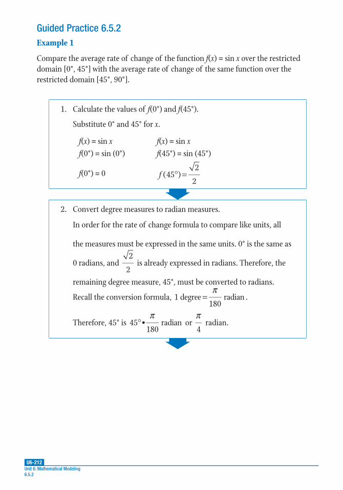
U6-212Unit 6: Mathematical Modeling6.5.2
Example 1
Compare the average rate of change of the function f(x) = sin x over the restricted domain [0°, 45°] with the average rate of change of the same function over the restricted domain [45°, 90°].
1. Calculate the values of f(0°) and f(45°).
Substitute 0° and 45° for x.
f(x) = sin x f(x) = sin x f(0°) = sin (0°) f(45°) = sin (45°)
f(0°) = 0 ° =f (45 )2
2
2. Convert degree measures to radian measures.
In order for the rate of change formula to compare like units, all
the measures must be expressed in the same units. 0° is the same as
0 radians, and 2
2 is already expressed in radians. Therefore, the
remaining degree measure, 45°, must be converted to radians.
Recall the conversion formula, π
=1 degree180
radian .
Therefore, 45° is π
°45 •180
radian or π4
radian.
Guided Practice 6.5.2

U6-213Lesson 5: Comparing Properties Within and Between Functions
6.5.2
3. Calculate the rate of change over the restricted domain [0°, 45°].
Substitute the results from the previous steps into the formula for the rate of change.
=−−
rf x f x
x x
( ) ( )1 2
1 2
Rate of change formula
π
( )
( )=
−
−
r
2
20
40
Substitute 2
2 for f1(x), 0 for f2(x),
π4
for x1, and 0 for x2.
π=r
4 2
2Simplify.
π=r
2 2
r ≈ 0.9
The rate of change over the restricted domain [0°, 45°] is approximately 0.9 radian.
4. Calculate the rate of change over the restricted domain [45°, 90°].
As determined in step 1, ° =f (45 )2
2.
Calculate the value of f(90°).
f(x) = sin x
f(90°) = sin (90°)
f(90°) = 1
Convert degree measures to radian measures.
As found in step 2, 45° is equal to π4
radian.(continued)

U6-214Unit 6: Mathematical Modeling6.5.2
Using the conversion formula, 90° is π
°90 •180
radian or π2
radians.
Substitute the results of the previous steps into the formula for the
rate of change.
=−−
rf x f x
x x
( ) ( )1 2
1 2
Rate of change formula
π π
( )=
−
−
r
2
21
4 2
Substitute 2
2 for f1(x), 1 for f2(x),
π4
for x1,
and π2
for x2.
π π=
−
−r
2 2
22
4
Simplify.
π( )
=−
−r
4 2 2
2Continue to simplify.
π( )
=−
r2 2 2
r ≈ 0.37
The rate of change over the restricted domain [45°, 90°] is approximately 0.37 radian.
5. Summarize the results of steps 1–4 for the two average rates of change for f(x) = sin x.
The function is increasing over both restricted domains. However, the rate of change of the increase is greater over the interval [0°, 45°] than over the interval [45°, 90°].

U6-215Lesson 5: Comparing Properties Within and Between Functions
6.5.2
Example 2
Two school clubs are selling plants to raise money for a trip. The juggling club started out with 250 plants and had 30 left after selling them for 7 days. The mock trial club started out with 450 plants and had 50 left after selling them for 8 days. Compare the rates at which the two clubs are selling their plants. If the two clubs started selling plants at the same time, which club will sell out of plants first? Explain.
1. Determine how many plants the juggling club has sold.
The juggling club has sold 250 – 30 or 220 plants.
2. Calculate the average number of plants the juggling club sold per day.
The juggling club sold 220 plants over 7 days. Divide to determine the average.
≈220
731
The juggling club sold an average of approximately 31 plants each day.
3. Determine how many plants the mock trial club has sold.
The mock trial club has sold 450 – 50 or 400 plants.
4. Calculate the average number of plants the mock trial club sold per day.
The mock trial club sold 400 plants over 8 days. Divide to determine the average.
=400
850
The mock trial club sold an average of 50 plants each day.

U6-216Unit 6: Mathematical Modeling6.5.2
5. Describe the rates at which the two clubs sold their plants. Compare the kinds of numbers that represent days, plants, and rates.
The variables “days” and “plants” are positive whole numbers, whereas “rate” can be a negative number. In this situation, the rates for the two clubs are negative, because the rates reflect a reduction in the number of plants each club has in stock. The rate for the juggling club is approximately –31 plants per day because the quantity of plants is being reduced by an average of about 31 per day; similarly, the rate for the mock trial club is –50 plants per day.
6. Calculate how long it will take the juggling club to sell its remaining plants.
The juggling club has 30 plants left and is selling them at a rate of about –31 plants per day, so the juggling club’s plants will sell out in 1 day.
7. Calculate how long it will take the mock trial club to sell its remaining plants.
The mock trial club has 50 plants left and is selling them at a rate of –50 plants per day, so the mock trial club’s plants will sell out in 1 day.
8. Explain which club will sell out of plants first.
Both clubs will sell off their remaining stock in 1 day. However, assuming each club started selling the plants on the same day, the juggling club will sell out first because it took 1 day less to sell off its initial stock of plants. (Recall that the juggling club sold plants for 7 days and the mock trial club sold plants for 8 days.)
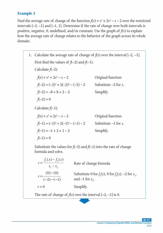
U6-217Lesson 5: Comparing Properties Within and Between Functions
6.5.2
Example 3
Find the average rate of change of the function f(x) = x3 + 2x2 – x – 2 over the restricted intervals [–2, –1] and [–1, 1]. Determine if the rate of change over both intervals is positive, negative, 0, undefined, and/or constant. Use the graph of f(x) to explain how the average rate of change relates to the behavior of the graph across its whole domain.
1. Calculate the average rate of change of f(x) over the interval [–2, –1].
First find the values of f(–2) and f(–1).
Calculate f(–2).
f(x) = x3 + 2x2 – x – 2 Original function
f(–2) = (–2)3 + 2(–2)2 – (–2) – 2 Substitute –2 for x.
f(–2) = –8 + 8 + 2 – 2 Simplify.
f(–2) = 0
Calculate f(–1).
f(x) = x3 + 2x2 – x – 2 Original function
f(–1) = (–1)3 + 2(–1)2 – (–1) – 2 Substitute –1 for x.
f(–1) = –1 + 2 + 1 – 2 Simplify.
f(–1) = 0
Substitute the values for f(–2) and f(–1) into the rate of change formula and solve.
=−−
rf x f x
x x
( ) ( )1 2
1 2
Rate of change formula
=−
− − −r
(0) (0)
( 2) ( 1)Substitute 0 for f1(x), 0 for f2(x), –2 for x1, and –1 for x2.
r = 0 Simplify.
The rate of change of f(x) over the interval [–2, –1] is 0.
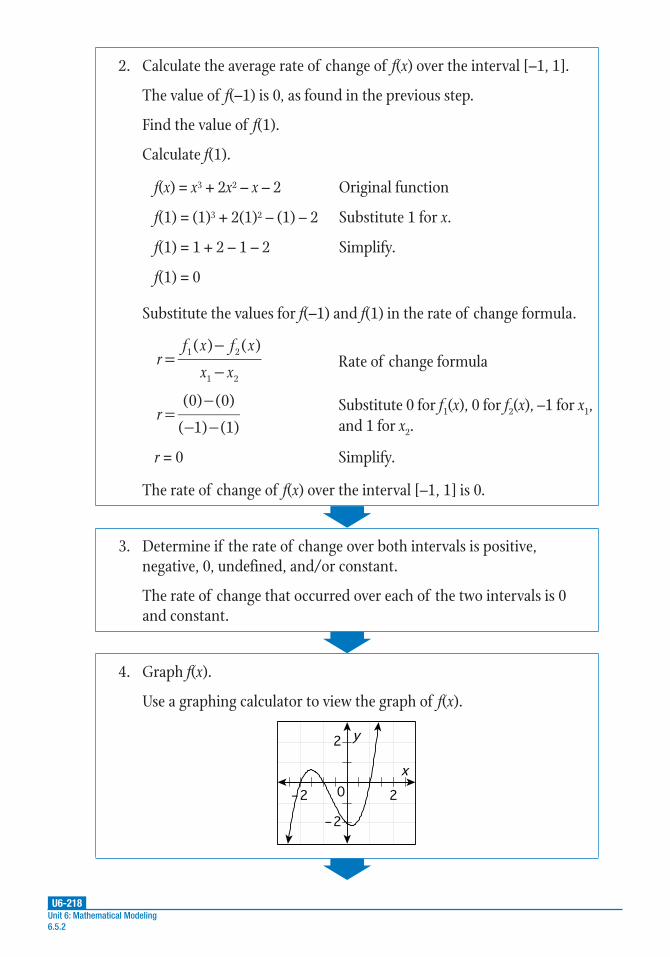
U6-218Unit 6: Mathematical Modeling6.5.2
2. Calculate the average rate of change of f(x) over the interval [–1, 1].
The value of f(–1) is 0, as found in the previous step.
Find the value of f(1).
Calculate f(1).
f(x) = x3 + 2x2 – x – 2 Original function
f(1) = (1)3 + 2(1)2 – (1) – 2 Substitute 1 for x.
f(1) = 1 + 2 – 1 – 2 Simplify.
f(1) = 0
Substitute the values for f(–1) and f(1) in the rate of change formula.
=−−
rf x f x
x x
( ) ( )1 2
1 2
Rate of change formula
=−
− −r
(0) (0)
( 1) (1)Substitute 0 for f1(x), 0 for f2(x), –1 for x1, and 1 for x2.
r = 0 Simplify.
The rate of change of f(x) over the interval [–1, 1] is 0.
3. Determine if the rate of change over both intervals is positive, negative, 0, undefined, and/or constant.
The rate of change that occurred over each of the two intervals is 0 and constant.
4. Graph f(x).
Use a graphing calculator to view the graph of f(x).
–2 20x
2
–2
y

U6-219Lesson 5: Comparing Properties Within and Between Functions
6.5.2
Example 4
Three linear functions—f(x), g(x), and h(x)—share a common intersection point of (1, 1) on a coordinate plane. The function f(x) also passes through the point (–2, –3), while the function g(x) passes through the point (–2, 3), and the function h(x) passes through the point (2, 3). Which function has the greatest rate of change? What are the equations of the functions?
1. Calculate the rate of change for f(x).
The rate of change formula can be applied to the two points that satisfy the function f(x): (1, 1) and (–2, –3).
=−−
rf x f x
x x
( ) ( )1 2
1 2
Rate of change formula
=− −− −
r(1) ( 3)
(1) ( 2)Substitute 1 for f1(x), –3 for f2(x), 1 for x1, and –2 for x2.
=r4
3Simplify.
The rate of change for f(x) is 4
3.
5. Describe what happens to the function values over the restricted domains [–2, –1] and [–1, 1].
The function value goes from 0 to a maximum value and back to 0 over the restricted domain [–2, –1].
The function value goes from 0 to a minimum value and back to 0 over the restricted domain [–1, –1]. For the domain interval ( , 2)−∞ − , the function value range is given by the interval ( ,0)−∞ ; for the domain interval (1, )+∞ , the function value range is given by the interval (0, )+∞ .
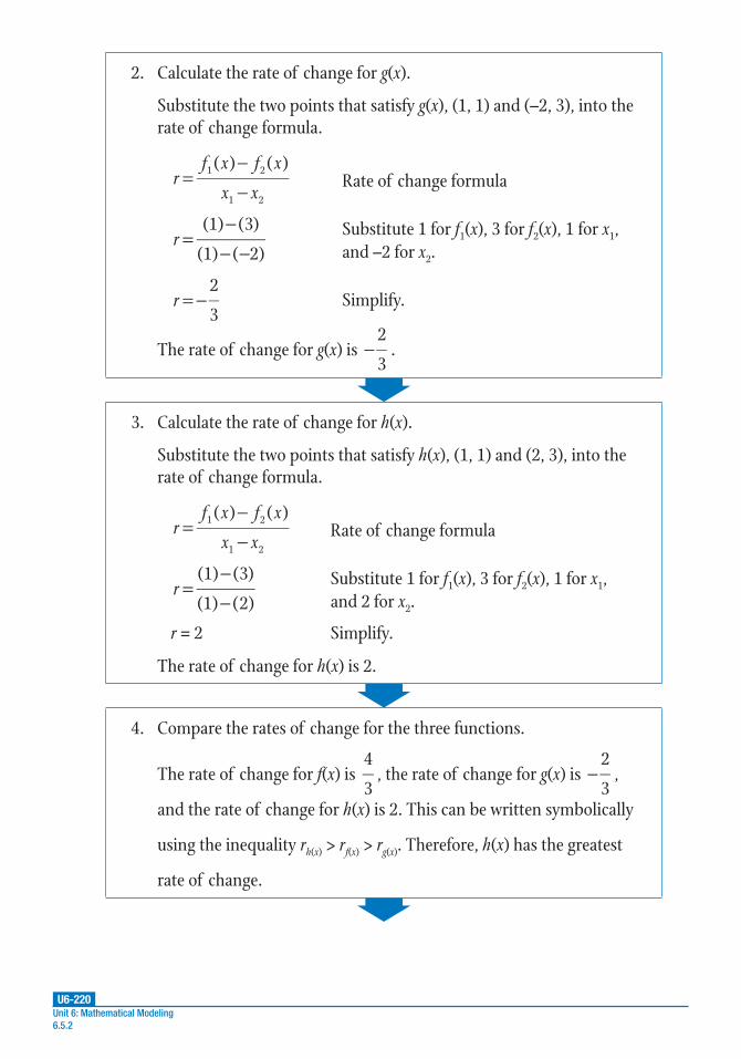
U6-220Unit 6: Mathematical Modeling6.5.2
2. Calculate the rate of change for g(x).
Substitute the two points that satisfy g(x), (1, 1) and (–2, 3), into the rate of change formula.
=−−
rf x f x
x x
( ) ( )1 2
1 2
Rate of change formula
=−− −
r(1) (3)
(1) ( 2)Substitute 1 for f1(x), 3 for f2(x), 1 for x1, and –2 for x2.
=−r2
3Simplify.
The rate of change for g(x) is −2
3.
3. Calculate the rate of change for h(x).
Substitute the two points that satisfy h(x), (1, 1) and (2, 3), into the rate of change formula.
=−−
rf x f x
x x
( ) ( )1 2
1 2
Rate of change formula
=−−
r(1) (3)
(1) (2)Substitute 1 for f1(x), 3 for f2(x), 1 for x1, and 2 for x2.
r = 2 Simplify.
The rate of change for h(x) is 2.
4. Compare the rates of change for the three functions.
The rate of change for f(x) is 4
3, the rate of change for g(x) is −
2
3,
and the rate of change for h(x) is 2. This can be written symbolically
using the inequality rh(x) > rf(x) > rg(x). Therefore, h(x) has the greatest
rate of change.

U6-221Lesson 5: Comparing Properties Within and Between Functions
6.5.2
5. Use the point-slope form of a linear equation to write the equation of each function.
The point-slope form of a linear equation is y – y1 = m(x – x1), in which m is the rate of change and x1 and y1 are coordinates of a point that makes the function a true statement. Use the shared point (1, 1) for the point for each function.
For f(x):
y – y1 = m(x – x1) Point-slope formula
( ) ( )− =
− f x x( ) 1
4
31 Substitute 1 for x1, 1 for y1, and
4
3 for m.
= −f x x( )4
3
1
3Simplify.
For g(x):
y – y1 = m(x – x1) Point-slope formula
( ) ( )− = −
− g x x( ) 1
2
31
Substitute 1 for x1, 1 for y1, and −2
3
for m.
=− +g x x( )2
3
5
3Simplify.
For h(x):
y – y1 = m(x – x1) Point-slope formula
h(x) – (1) = (2)[x – (1)] Substitute 1 for x1, 1 for y1, and 2 for m.
h(x) = 2x – 1 Simplify.
The equations for the three functions are = −f x x( )4
3
1
3,
=− +g x x( )2
3
5
3, and h(x) = 2x – 1.

U6-222Unit 6: Mathematical Modeling6.5.2
Example 5
The table gives the function values for f(x) = log x over the restricted domain [0.001, 1,000]. Use the data to calculate and compare the rates of change of f(x) for the intervals [0.001, 0.01], [0.01, 0.1], [0.1, 1], and [1, 10]. Describe how the rates change as the values of x become larger and smaller.
x 0.001 0.01 0.1 1 10 100 1,000f(x) –3 –2 –1 0 1 2 3
1. Calculate the rate of change of f(x) over the interval [0.001, 0.01].
Substitute the table values for x and f(x) into the concise form of the
rate of change formula, rf x
x
�
�
( )= .
rf x
x
�
�
( )= Concise form of the rate of
change formula
=− − −
−r
( 3) ( 2)
(0.001) (0.01)Substitute (–3) – (–2) for Df(x) and (0.001) – (0.01) for Dx.
=−
−r
1
0.009Simplify.
=r 111.1
The rate of change of f(x) over the interval [0.001, 0.01] is 111.1 .
2. Calculate the rate of change of f(x) over the interval [0.01, 0.1].
Substitute the table values for x and f(x) into rf x
x
�
�
( )= .
rf x
x
�
�
( )= Formula
=− − −
−r
( 2) ( 1)
(0.01) (0.1)Substitute (–2) – (–1) for Df(x) and (0.01) – (0.1) for Dx.
=−
−r
1
0.09Simplify.
=r 11.1
The rate of change of f(x) over the interval [0.01, 0.1] is 11.1 .

U6-223Lesson 5: Comparing Properties Within and Between Functions
6.5.2
3. Calculate the rate of change of f(x) over the interval [0.1, 1].
Substitute the table values for x and f(x) into rf x
x
�
�
( )= .
rf x
x
�
�
( )= Formula
=− −
−r
( 1) (0)
(0.1) (1)Substitute (–1) – (0) for Df(x) and (0.1) – (1) for Dx.
=−−
r1
0.9Simplify.
=r 1.1
The rate of change of f(x) over the interval [0.1, 1] is 1.1 .
4. Calculate the rate of change of f(x) over the interval [1, 10].
Substitute the table values for x and f(x) into rf x
x
�
�
( )= .
rf x
x
�
�
( )= Formula
=−−
r(0) (1)
(1) (10)Substitute (0) – (1) for Df(x) and (1) – (10) for Dx.
=−−
r1
9Simplify.
=r 0.1
The rate of change of f(x) over the interval [1, 10] is 0.1 .
5. Describe how the rate of change will change as the values of the domain interval increase.
Compare the rate of change r for each interval of interest for f(x):
• For [0.001, 0.01], r = 111.1 .
• For [0.01, 0.1], r = 11.1 .
• For [0.1, 1], r = 1.1 .
• For [1, 10], r = 0.1 .
As the values of x increase, the rate of change decreases.
U6-224
PRACTICE
UNIT 6 • MATHEMATICAL MODELINGLesson 5: Comparing Properties Within and Between Functions
Unit 6: Mathematical Modeling6.5.2
For problems 1–4, find the average rate of change between x = 0 and x = 1 for the function given.
1. a(x) = 2x – x2
2. b(x) = x3 – 3x
3. c(x) = sin (x – 1)
4. d(x) = –cos (1 – x)
For problems 5–7, determine the average rate of change r over the domain intervals [–2, –1] and [–1, 0] for the function given.
5. =−
f xx
x( )
1
6. g(x) = sin 2x
7. h(x) = log (x + 3)
Practice 6.5.2: Calculating Average Rates of Change
continued

U6-225
PRACTICE
UNIT 6 • MATHEMATICAL MODELINGLesson 5: Comparing Properties Within and Between Functions
Lesson 5: Comparing Properties Within and Between Functions6.5.2
The following graph shows the amount of nitrogen fertilizer needed to produce the leaves and stems of two different varieties of corn for use as biofuel stock. The function f(x) represents one variety, and the function g(x) represents the other. Over the “leaf ” interval [0, 2.25], the plant uses the nitrogen mostly for growing the leaves. Over the “stem” interval [2.25, 9], the plant uses the nitrogen mostly for growing the stems, which are of the most use in producing biofuel. Use the graph to complete problems 8–10.
2 4 6 8 10 12 14 16 18
x
200
190
180
170
160
150
140
130
120
110
100
90
80
70
60
50
40
30
20
10
0
y
f(x)
g(x)
Yield (metric tons/hectare)
Nit
rog
en (k
ilog
ram
s/h
ecta
re)
8. Compare the average rates of change of the fertilizer needed for the two different corn varieties represented by the graphs of f(x) and g(x) over the “leaf ” interval.
9. Compare the average rates of change of the fertilizer needed for the two different corn varieties represented by the graphs of f(x) and g(x) over the “stem” interval.
10. Which variety of corn would most likely be preferred by biofuel producers? Why?
U6-226Unit 6: Mathematical Modeling6.5.3
Introduction
Functions can be compared for a variety of purposes. Functions of the same type—for example, quadratic functions—can be compared on the basis of maximum or minimum function values, symmetry about an axis or other vertical line on the coordinate plane, or on the basis of how well the function fits real-world data.
Functions of different types—such as polynomial functions and rational functions—can likewise be compared on the basis of one or more characteristics, such as the number of real solutions or the rate of change over a restricted domain interval.
Key Concepts
• The function characteristics that are used to compare and contrast function types can depend on the purpose of the comparison.
• Recall that the extrema of a function, or the points on a graph of a function at which a maximum or minimum function value occurs, can apply to the function across its entire domain or they can be localized, as in the case of polynomial functions of degree three and higher.
• For example, a cubic equation might be used to model a real-world problem that has a single solution. Graphing a proposed model for the problem can quickly show whether the model meets the criteria of having only one real solution.
• The rate of change of a function value can be calculated to determine which of several different functions (or functions of the same form) best represent a condition of decreasing or increasing function values.
• The symmetry exhibited by a function can be about a vertical line on a coordinate plane or it can be exhibited across a line of symmetry that takes the form of a linear function.
• Symmetry of domain and function values can also be observed in the algebraic form of a function, such as in even or odd functions.
• Domains and ranges can also be used to compare the validity of a function serving as a model for real-world phenomena. In some cases, only a restricted domain or range of a mathematical model is relevant to a specific problem.
• A function’s behavior at domain values that are very large or small can be relevant to some real-world problems. Functions might serve as reliable models over a narrowly restricted mathematical domain, but might fail to describe real-world phenomena when domain values increase or decrease by large values.
Lesson 6.5.3: Comparing Functions

U6-227Lesson 5: Comparing Properties Within and Between Functions
6.5.3
Example 1
Two functions f(x) = –2(x – 5)2 + 3 and g(x) = –4x2 + 8x + 3 each represent the volume of a rectangular solid. Which solid’s function, f(x) or g(x), has the greater maximum volume?
1. Determine the coordinates of the maximum point of f(x).
To determine the coordinates of the maximum point of a function, first determine the type of function and compare it to the standard form for that function.
The function f(x) = –2(x – 5)2 + 3 is a quadratic function.
The vertex form for a quadratic function is f(x) = a(x – h)2 + k, where the coordinates of the maximum (a < 0) or minimum (a > 0) function value are (h, k).
Since f(x) = –2(x – 5)2 + 3 is already written in vertex form, it can be seen that for f(x), h = 5, k = 3 and a = –2, which is less than 0; therefore, the maximum point of f(x) is located at (5, 3).
2. Determine the coordinates of the maximum point of g(x).
g(x) = –4x2 + 8x + 3 is also a quadratic function, but it is written in standard form, f(x) = ax2 + bx + c, where a = –4, b = 8, and c = 3.
Recall that the x-coordinate of the maximum or minimum of a
quadratic in this form is =−xb
a2.
=−xb
a2Formula for the x-coordinate
=−−
x(8)
2( 4)Substitute –4 for a and 8 for b.
=−−
x8
8Simplify.
x = 1
(continued)
Guided Practice 6.5.3
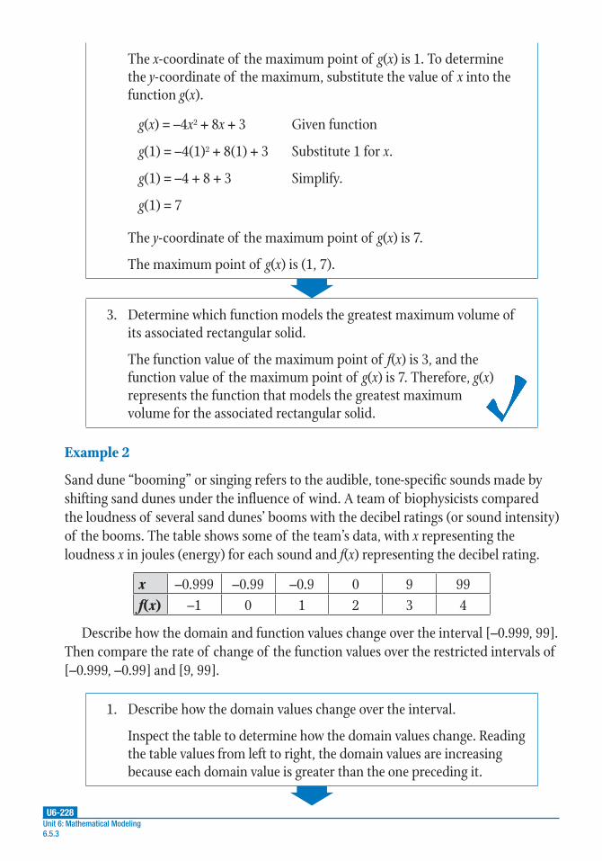
U6-228Unit 6: Mathematical Modeling6.5.3
The x-coordinate of the maximum point of g(x) is 1. To determine the y-coordinate of the maximum, substitute the value of x into the function g(x).
g(x) = –4x2 + 8x + 3 Given function
g(1) = –4(1)2 + 8(1) + 3 Substitute 1 for x.
g(1) = –4 + 8 + 3 Simplify.
g(1) = 7
The y-coordinate of the maximum point of g(x) is 7.
The maximum point of g(x) is (1, 7).
3. Determine which function models the greatest maximum volume of its associated rectangular solid.
The function value of the maximum point of f(x) is 3, and the function value of the maximum point of g(x) is 7. Therefore, g(x) represents the function that models the greatest maximum volume for the associated rectangular solid.
Example 2
Sand dune “booming” or singing refers to the audible, tone-specific sounds made by shifting sand dunes under the influence of wind. A team of biophysicists compared the loudness of several sand dunes’ booms with the decibel ratings (or sound intensity) of the booms. The table shows some of the team’s data, with x representing the loudness x in joules (energy) for each sound and f(x) representing the decibel rating.
x –0.999 –0.99 –0.9 0 9 99f(x) –1 0 1 2 3 4
Describe how the domain and function values change over the interval [–0.999, 99]. Then compare the rate of change of the function values over the restricted intervals of [–0.999, –0.99] and [9, 99].
1. Describe how the domain values change over the interval.
Inspect the table to determine how the domain values change. Reading the table values from left to right, the domain values are increasing because each domain value is greater than the one preceding it.

U6-229Lesson 5: Comparing Properties Within and Between Functions
6.5.3
2. Describe how the function values (or range) change over the domain interval.
The function or range values increase at a constant rate of 1 unit for each of the domain values.
3. Calculate the rate of change for the intervals [–0.999, –0.99] and [9, 99].
Substitute the table values for x and f(x) into the concise form of the
rate of change formula, rf x
x
�
�
( )= .
For the interval [–0.999, –0.99]:
rf x
x
�
�
( )= Concise formula for the rate of change
=− −
−r
( 1) (0)
( 0.999) – (–0.99)Substitute (–1) – (0) for Df(x) and (–0.999) – (–0.99) for Dx.
=−
−r
1
0.009Simplify.
=r 111.1
The rate of the change for the interval [–0.999, –0.99] is 111.1 .
For the interval [9, 99]:
rf x
x
�
�
( )= Concise formula for the rate of change
=−−
r(3) (4)
(9) (99)Substitute (3) – (4) for Df(x) and (9) – (99) for Dx.
=−−
r1
90Simplify.
=r 0.01
The rate of the change for the interval [9, 99] is 0.01 .

U6-230Unit 6: Mathematical Modeling6.5.3
Example 3
Use the data from the table in Example 2 (shown in the table that follows) to find the function that fits the data if the general form of the function is f(x) = a + log (x + b).
x –0.999 –0.99 –0.9 0 9 99f(x) –1 0 1 2 3 4
1. Determine the number of data points that will be needed to find the function.
The general form has four variables—a, b, f(x), and x. However, each data point has both an x and an f(x) value, which leaves two unknowns, a and b. Therefore, two equations in a and b will be needed to find the function.
2. Pick two points from the table and substitute them into the general form of the function to write equations for the points.
Any two points can be chosen. Let the two points be (9, 3) and (99, 4).
For (9, 3):
f(x) = a + log (x + b) General form
(3) = a + log [(9) + b] Substitute 9 for x and 3 for f(x).
3 = a + log (9 + b) Simplify.
(continued)
4. Compare the rates of change of the function values for the two intervals.
Both rates of change are positive, but the rate of change over the interval [–0.999, –0.99] is 10,000 times greater than the rate of change over the interval [9, 99].

U6-231Lesson 5: Comparing Properties Within and Between Functions
6.5.3
For (99, 4):
f(x) = a + log (x + b) General form
(4) = a + log [(99) + b] Substitute 99 for x and 4 for f(x).
4 = a + log (99 + b) Simplify.
The equations for the data points (9, 3) and (99, 4) are 3 = a + log (9 + b) and 4 = a + log (99 + b).
3. Use the resulting equations to eliminate one of the unknown variables (a or b).
Either variable can be eliminated; let’s eliminate a.
To eliminate a, subtract one equation from the other.
[4 = a + log (99 + b)] – [3 = a + log (9 + b)]Set up the subtraction equation.
1 = log (99 + b) – log (9 + b) Subtract like terms.
=++
b
b1 log
99
9
Simplify using the quotient rule of logarithms.
=++
b
b10
99
91
Simplify using the definition of a common logarithm.
10 • (9 + b) = 99 + b Multiply both sides by (9 + b).
90 + 10b = 99 + b Distribute.
10b = 9 + bSubtract 90 from both sides.
9b = 9 Subtract b from both sides.
b = 1 Divide by 9.
The value of b is 1.
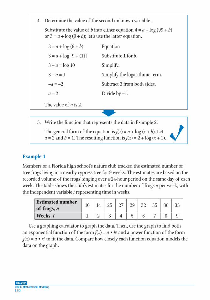
U6-232Unit 6: Mathematical Modeling6.5.3
4. Determine the value of the second unknown variable.
Substitute the value of b into either equation 4 = a + log (99 + b) or 3 = a + log (9 + b); let’s use the latter equation.
3 = a + log (9 + b) Equation
3 = a + log [9 + (1)] Substitute 1 for b.
3 – a = log 10 Simplify.
3 – a = 1 Simplify the logarithmic term.
–a = –2 Subtract 3 from both sides.
a = 2 Divide by –1.
The value of a is 2.
5. Write the function that represents the data in Example 2.
The general form of the equation is f(x) = a + log (x + b). Let a = 2 and b = 1. The resulting function is f(x) = 2 + log (x + 1).
Example 4
Members of a Florida high school’s nature club tracked the estimated number of tree frogs living in a nearby cypress tree for 9 weeks. The estimates are based on the recorded volume of the frogs’ singing over a 24-hour period on the same day of each week. The table shows the club’s estimates for the number of frogs n per week, with the independent variable t representing time in weeks.
Estimated number of frogs, n
10 14 25 27 29 32 35 36 38
Weeks, t 1 2 3 4 5 6 7 8 9
Use a graphing calculator to graph the data. Then, use the graph to find both an exponential function of the form f(x) = a • bx and a power function of the form g(x) = a • xb to fit the data. Compare how closely each function equation models the data on the graph.

U6-233Lesson 5: Comparing Properties Within and Between Functions
6.5.3
1. Create a scatter plot of the table values using a graphing calculator.
Follow the instructions appropriate to your calculator model.
On a TI-83/84:
Step 1: Press [STAT] to bring up the statistics menu. The first option, 1: Edit, will already be highlighted. Press [ENTER].
Step 2: Arrow up to L1 and press [CLEAR], then [ENTER], to clear the list (or repeatedly hit the [DEL] key until all old data is deleted). Repeat this process to clear L2 and L3 if needed.
Step 3: From L1, press the down arrow to move your cursor into the list. Enter each t value from the table into L1, pressing [ENTER] after each number to navigate down to the next blank spot in the list.
Step 4: Arrow over to L2 and enter the n values as listed in the table.
Step 5: Press [GRAPH] to see how n varies with t.
Step 6: To adjust the viewing window, press [WINDOW]. Choose settings as appropriate; for example, the x-axis could run from 1 to 10 and the y-axis could run from 0 to 40.
On a TI-Nspire:
Step 1: Press [home]. Arrow over to the spreadsheet icon, the fourth icon from the left, and press [enter].
Step 2: To clear the lists in your calculator, arrow up to the topmost cell of the table to highlight the entire column, then press [menu]. Use the arrow key to choose 3: Data, then 4: Clear Data, then press [enter]. Repeat for each column as necessary.
Step 3: Select the top cell in column A and enter “t” since it is the independent variable. Then select the top cell in column B and enter “n” for the dependent variable.
Step 4: Enter the ordered pairs in the cells A1 through A9 and B1 through B9.
Step 5: To see the graph, press [menu], and then select 3: Graph Type and 4: Scatter Plot.
Step 6: Select “t” from the x pop-up menu and “n” from the y pop-up menu to see the points.
(continued)

U6-234Unit 6: Mathematical Modeling6.5.3
Step 7: To adjust the viewing window, press [menu] and then select 4: Window/Zoom and 1: Window Settings. Choose settings as appropriate; for example, the x-axis could run from 1 to 10 and the y-axis could run from 0 to 40.
The resulting scatter plot should resemble the following.
2 4 6 8 10
t
40
38
36
34
32
30
28
26
24
22
20
18
16
14
12
10
8
6
4
2
0
n
2. Next, use the graphing calculator to fit the data to an exponential function and a power function.
Follow the instructions appropriate to your calculator model. Round the values for a and b to two significant figures.
On a TI-83/84:
Step 1: Press [STAT] and arrow over to the CALC menu.
Step 2: For an exponential function, arrow down to 0: ExpReg. Press [ENTER]. Enter the L1 variable ([2ND][1]) followed by a comma [,] and the L2 variable ([2ND][2]). Press [ENTER]. The results will be in the form f(x) = a • bx, with a ≈ 12 and b ≈ 1.2.
Step 3: For a power function, select A: PwrReg from the CALC menu as described in Step 1. Repeat Step 2. The results will be in the form g(x) = a • xb, with a ≈ 10 and b ≈ 0.6.
(continued)

U6-235Lesson 5: Comparing Properties Within and Between Functions
6.5.3
On a TI-Nspire:
Step 1: Go back to the data table for n and t. Press [menu] and select 4: Statistics and then 1: Stat Calculations.
Step 2: For an exponential function, select A: Exponential Regression.
Step 3: For X List, select the t variable from the pop-up menu. For Y List, select the n variable from the pop-up menu. Tab to “OK” to see the equation of the function.
Step 4: The results will be in the form f(x) = a • bx, with a ≈ 12 and b ≈ 1.2.
Step 5: For a power function, repeat Step 1, then select 9: Power Regression from the Stat Calculations menu.
Step 6: Repeat Step 3.
Step 7: The results will be in the form g(x) = a • xb, with a ≈ 10 and b ≈ 0.6.
3. Write the equations of the calculated exponential and power functions from using the variables n and t.
Substitute n, t, and the rounded values for a and b into the general form of each type of function.
Exponential function f(x) = a • bx
Power function g(x) = a • xb
TI-83/84 n(t) = 12 • (1.2)t n(t) = 10 • t0.6 TI-Nspire n(t) = 12 • (1.2)t n(t) = 10 • t0.6

U6-236Unit 6: Mathematical Modeling6.5.3
4. Plot the exponential and power functions from the previous step on the scatter plots produced by the tree-frog data.
Return to your graph of the scatter plot and enter the equations for the functions f(x) and g(x) from step 3 to add them to the graph. The resulting combined graph should resemble the following.
2 4 6 8 10
t
40
38
36
34
32
30
28
26
24
22
20
18
16
14
12
10
8
6
4
2
0
n
n(t) = 12 • (1.2)t
n(t) = 10 • t0.6
5. Describe how well the exponential function fits the data points.
The exponential function n(t) = 12 • (1.2)t best fits the data from about t = 3 to t = 6. Before t = 3, the exponential function value is greater than the scatter plot function values. For t > 6, the exponential function values diverge from and are greater than the scatter plot function values.
6. Describe how well the power function fits the data points.
The power function n(t) = 10 • t0.6 approximately fits the data from t = 1 to t = 9. The power function values are consistently less than the scatter plot function values from t = 3 to t = 9, but they follow the trend of the increasing scatter plot function values.
7. Determine which function type, exponential or power, best fits the data.
The function values of the power function n(t) = 10 • t0.6 fit the scatter plot data better over this domain interval [1, 9].
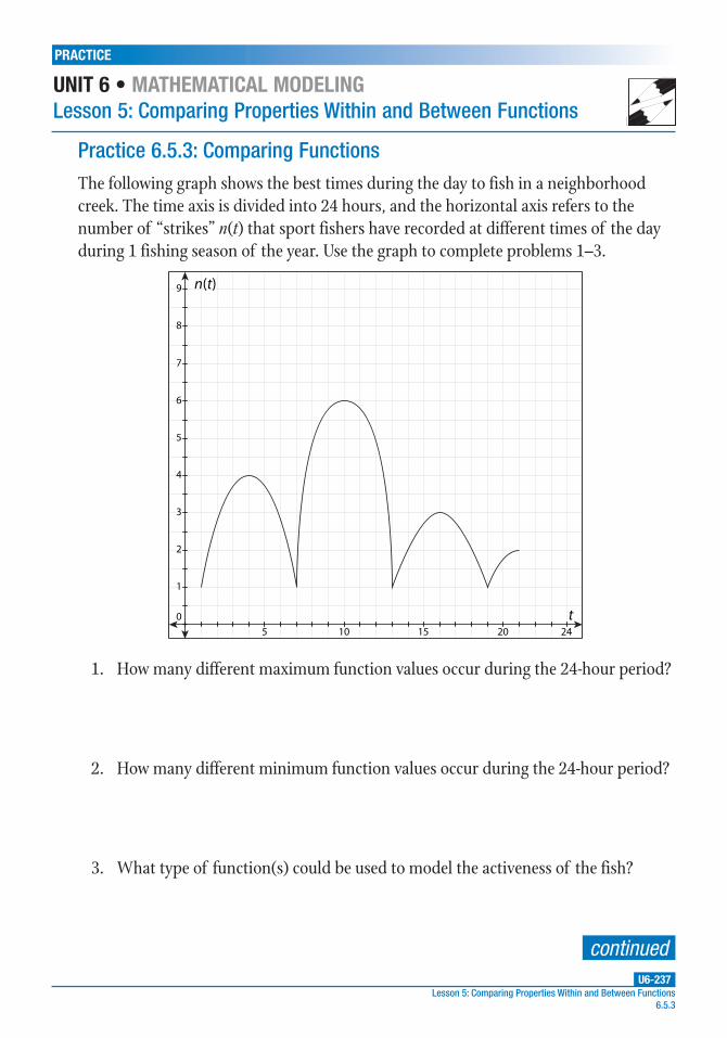
U6-237
PRACTICE
UNIT 6 • MATHEMATICAL MODELINGLesson 5: Comparing Properties Within and Between Functions
Lesson 5: Comparing Properties Within and Between Functions6.5.3
The following graph shows the best times during the day to fish in a neighborhood creek. The time axis is divided into 24 hours, and the horizontal axis refers to the number of “strikes” n(t) that sport fishers have recorded at different times of the day during 1 fishing season of the year. Use the graph to complete problems 1–3.
5 10 15 20 24
9
8
7
6
5
4
3
2
1
0 t
n(t)
1. How many different maximum function values occur during the 24-hour period?
2. How many different minimum function values occur during the 24-hour period?
3. What type of function(s) could be used to model the activeness of the fish?
Practice 6.5.3: Comparing Functions
continued

U6-238
PRACTICE
UNIT 6 • MATHEMATICAL MODELINGLesson 5: Comparing Properties Within and Between Functions
Unit 6: Mathematical Modeling6.5.3
Use the following information for problems 4–7.
Bansi, Josh, and Penn are tossing driftwood pieces off of Flat Rock Point, a cliff-top overlook point on the California coast. It takes the driftwood 5 seconds to fall to the rocks in the Pacific Ocean below.
4. Find the average vertical rate of change of Bansi’s driftwood over the time interval [1, 1.01] if the function describing the vertical distance Bansi’s throw travels is B(t) = –16t2 + 5t.
5. Find the average vertical rate of change of Josh’s driftwood over the time interval [1, 1.01] if the function describing the vertical distance Josh’s throw travels is J(t) = –16t2 + 4t.
6. Find the average vertical rate of change of Penn’s driftwood over the time interval [1, 1.01] if the function describing the vertical distance Penn’s throw travels is P(t) = –16t2 + 3t.
7. What do the results of problems 4–6 imply about how to calculate the average vertical rate of change of the driftwood at any time t? Write a function for the average vertical rate of change or speed.
continued

U6-239
PRACTICE
UNIT 6 • MATHEMATICAL MODELINGLesson 5: Comparing Properties Within and Between Functions
Lesson 5: Comparing Properties Within and Between Functions6.5.3
For problems 8–10, find the domain interval over which the rates of change of the two functions are equal. Use the interval [x, x + k] to calculate the rate of change.
8. a(x) = ex; b(x) = 2 – ee
9. c(x) = log x; d(x) = log (x – 10)
10. e(x) = 2x; f(x) = x2

Lesson 6: Operating on FunctionsUNIT 6 • MATHEMATICAL MODELING
U6-240Unit 6: Mathematical Modeling 6.6
Common Core Georgia Performance Standards
MCC9–12.F.BF.1b★
MCC9–12.F.BF.1c★ (+)
Essential Questions
1. Why is it advantageous to represent functions in multiple ways (e.g., with data tables, equations, and graphs)?
2. Why is it important to consider the context of a problem when determining the domain of a function?
3. What is the process of adding or subtracting two functions?
4. What is the process of multiplying or dividing two functions?
5. How is the domain of the result of a composition of functions different from the individual domains of the functions themselves?
WORDS TO KNOW
addition function the result of adding two or more functions
combination of functions the process of combining two or more functions using the operations of addition, subtraction, multiplication, or division to create a new function
composite function the function that results from composing two separate functions, f(x) and g(x), so that the output of g(x) is the input of f(x), or vice versa. The composite function denoted by f(g(x)) is the result of composing f(x) and g(x).
composition of functions the process of substituting one function for the independent variable of another function to create a new function
product function the result of multiplying two or more functions
quotient function the result of dividing two functions
subtraction function the result of subtracting two or more functions
U6-241Lesson 6: Operating on Functions
6.6
Recommended Resources
• LearnZillion.com. “Combining Functions by Adding and Subtracting.”
http://www.walch.com/rr/00273
This video presentation illustrates the creation of a new function through adding two other functions.
• MathIsFun.com. “Composition of Functions.”
http://www.walch.com/rr/00274
This site offers step-by-step examples of how to compose functions, how to find the domain of the result, and how to check your work. Interactive practice questions at the bottom of the page provide detailed feedback.
• Purplemath.com. “Operations on Functions.”
http://www.walch.com/rr/00275
This website gives a detailed review of performing addition, subtraction, multiplication, and division on functions. An optional interactive widget allows users to input and solve function operations, and provides the answers; however, to see the steps leading up to the solution, users must sign up for a free Mathway account.

U6-242Unit 6: Mathematical Modeling 6.6.1
Lesson 6.6.1: Adding, Subtracting, Multiplying, and Dividing FunctionsIntroduction
A variety of functions can be used to model many different situations involving relationships between two quantities. For example, whereas linear functions are ideal for modeling relationships of quantities with constant rates of change, exponential functions are better for modeling relationships with rapid rates of change between variables. In some cases, it may be necessary to combine functions to describe more complicated relationships. The combination of functions refers to the process of combining two or more functions using the operations of addition, subtraction, multiplication, or division to create a new function. By learning how to combine functions algebraically, we can create functions that are more appropriate for a given situation in order to analyze the variables involved. Performing operations on functions is similar to operations with polynomials because functions consist of polynomials.
Key Concepts
Adding and Subtracting Functions
• The addition of two or more functions can be given by an addition function, (f1 + f2)(x) or f1(x) + f2(x) + f3(x) + … + fn(x), where each function may be of any degree.
• The subtraction of two or more functions can be written similarly as a subtraction function, (f1 – f2)(x) or f1(x) – f2(x) – f3(x) – … – fn(x), where each function may be of any degree.
• Adding or subtracting two functions f(x) and g(x) can be written as (f + g)(x) or (f – g)(x), respectively.
• When adding or subtracting functions, the degree of the resulting combined function is equal to the highest degree of the polynomials involved.
• For instance, the degree of the sum of f(x) = 3x + 1 and g(x) = 2x2 + 5x – 6 will be degree 2, because that is the highest degree of the two polynomials being added.
• Recall that the domain of a function is the set of all input values, or x-values, that satisfy the given function without restriction.
• The domain of an addition or subtraction function is the same as the domain of the individual functions.

U6-243Lesson 6: Operating on Functions
6.6.1
Multiplying Functions
• The multiplication of two or more functions can be given by a product function, (f1 • f2)(x) or f1(x) • f2(x) • f3(x) • … • fn(x), where each function may be of any degree.
• Multiplying two functions f(x) and g(x) can be written as (f • g)(x).
• In terms of the degree of the resulting product function, the multiplication of functions is a bit different from that of addition and subtraction functions.
• Recall that by the properties of exponents, am • an = am + n. Therefore, when two functions of any degree are multiplied, their exponents are added, so the degree of the resulting product function will always be higher than the degrees of the two original functions.
• If the two functions are linear, the resulting product is a quadratic with degree 2 and is obtained by using the Distributive Property of Multiplication.
• For example, if f(x) = x + 5 and g(x) = x, then the resulting product function (f • g)(x) will be (x + 5)(x) or x2 + 5x, which is a quadratic.
• If multiplying a linear function with a degree of 1 and a quadratic function with a degree of 2, then the resulting product function is a cubic function with a degree of 3.
• The domain of a product function is the same as the domain of the individual functions.
Dividing Functions
• The division of two functions, f1(x) and f2(x), results in a quotient function,
( )1
2
f
fx or
( )
( )1
2
f x
f x. Again, the involved functions may be of any degree.
• Dividing two functions f(x) and g(x) can be written as ( )
( )
f x
g x.
• When dividing two functions, determine whether one or both functions are
factorable. If so, use factoring techniques to simplify the numerator and/
or denominator. If neither function is factorable, leave the final quotient

U6-244Unit 6: Mathematical Modeling 6.6.1
with variables in the denominator. If factoring is not required, then subtract
the powers of the functions in the numerator and denominator to simplify
the quotient completely. For example, if f1(x) = 9x2 and f2(x) = x, then
( )
( )
99 91
2
22 1= = =−f x
f x
x
xx x . (Recall that by the Quotient of Powers Property of
exponents, = −a
aa
m
nm n .)
• The domain of a quotient function typically contains fewer values than the individual functions.
• For example, if f1(x) = x + 2 and f2(x) = x2 – 4, then the quotient function
( )
( )1
2
f x
f x would be
( )
( )
2
41
22=+−
f x
f x
x
x. When simplified, the quotient function
results in ( )
( )
2
( 2)( 2)
1
21
2
=+
+ −=
−f x
f x
x
x x x, which has a domain of all real
numbers except for x = 2 and x = –2, because those two values result in one
or the other of the factors of the denominator being equal to 0. When you
factor and cancel a common factor, you algebraically prove that there is a
hole in the graph—a removable point discontinuity. Therefore, both the
x- and y-coordinates for this point must be removed from the domain and
range, respectively.
• For ( )
( )
1
21
2
=−
f x
f x x, at x = 2, the denominator is 0, and so the function is
undefined. This domain contains fewer numbers than the domains of the
original functions, f1(x) = x + 2 and f2(x) = x2 – 4, which have a domain of all
real numbers.

U6-245Lesson 6: Operating on Functions
6.6.1
• In some cases, the resulting quotient function from two functions f1(x)
and f2(x) does not have variables in the denominator. For example, if
f1(x) = x2 + 5x + 6 and f2(x) = x + 3, then the quotient function ( )
( )1
2
f x
f x would be
( )
( )
5 6
3
( 3)( 2)
321
2
2
=+ ++
=+ +
+= +
f x
f x
x x
x
x x
xx . Again, the common factor x + 3,
which was canceled out, gives the x-value that is not in the domain of the
function due to a removable point discontinuity occurring at this value. If
x + 3 = 0, then x = –3 would not be found in the domain of this function.
• This table shows how two functions f(x) and g(x) can be combined through addition, subtraction, multiplication, or division to produce a new function h(x).
Combining f (x) and g(x) Using Operations
Combination Descriptionh(x) = (f + g)(x) (f + g)(x) = f(x) + g(x); also, (f + g)(x) = (g + f )(x) = g(x) + f(x)h(x) = (f – g)(x) (f – g)(x) = f(x) – g(x); (f – g)(x) ≠ (g – f )(x)h(x) = (g – f)(x) (g – f )(x) = g(x) – f(x); (g – f )(x) ≠ (f – g)(x) h(x) = (f • g)(x) (f • g)(x) = f(x) • g(x); also, (f • g)(x) = (g • f )(x) = g(x) • f(x)
h xf
gx( ) ( )=
f
gx
f x
g x
f
gx
g
fx( )
( )
( ); ( ) ( )
=
≠
=
h xg
fx( ) ( )
g
fx
g x
f x( )
( )
( );
= g
fx
f
gx( ) ( )
≠

U6-246Unit 6: Mathematical Modeling 6.6.1
Guided Practice 6.6.1Example 1
Given f(x) = –2x2 – 2x + 1 and g(x) = x + 1, find (f + g)(x), (f – g)(x), (f • g)(x), and ( )
( )
f x
g x.
1. Find (f + g)(x).
To find (f + g)(x), add the polynomials of the two functions, f(x) = –2x2 – 2x + 1 and g(x) = x + 1.
(f + g)(x) = f(x) + g(x)Write (f + g)(x) as the addition of two separate functions.
(f + g)(x) = (–2x2 – 2x + 1) + (x + 1)Substitute –2x2 – 2x + 1 for f(x) and x + 1 for g(x).
(f + g)(x) = –2x2 – x + 2 Combine like terms.
The result of (f + g)(x) is –2x2 – x + 2.
2. Find (f – g)(x).
To find (f – g)(x), subtract the polynomial of g(x) = x + 1 from that of f(x) = –2x2 – 2x + 1.
(f – g)(x) = f(x) – g(x)Write (f – g)(x) as the subtraction of two separate functions.
(f – g)(x) = (–2x2 – 2x + 1) – (x + 1)Substitute –2x2 – 2x + 1 for f(x) and x + 1 for g(x).
(f – g)(x) = –2x2 – 2x + 1 – x – 1 Simplify the subtraction.
(f – g)(x) = –2x2 – 3x Combine like terms.
The result of (f – g)(x) is –2x2 – 3x.
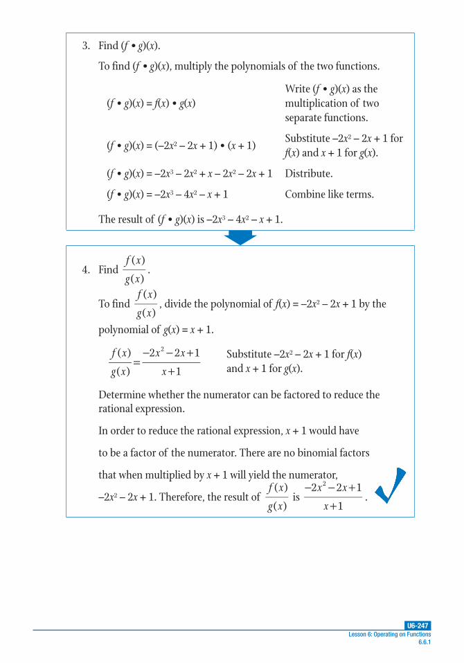
U6-247Lesson 6: Operating on Functions
6.6.1
3. Find (f • g)(x).
To find (f • g)(x), multiply the polynomials of the two functions.
(f • g)(x) = f(x) • g(x)Write (f • g)(x) as the multiplication of two separate functions.
(f • g)(x) = (–2x2 – 2x + 1) • (x + 1)Substitute –2x2 – 2x + 1 for f(x) and x + 1 for g(x).
(f • g)(x) = –2x3 – 2x2 + x – 2x2 – 2x + 1 Distribute.
(f • g)(x) = –2x3 – 4x2 – x + 1 Combine like terms.
The result of (f • g)(x) is –2x3 – 4x2 – x + 1.
4. Find ( )
( )
f x
g x.
To find ( )
( )
f x
g x, divide the polynomial of f(x) = –2x2 – 2x + 1 by the
polynomial of g(x) = x + 1.
( )
( )
2 2 1
1
2
=− − +
+f x
g x
x x
x Substitute –2x2 – 2x + 1 for f(x)
and x +
1
for g(x).
Determine whether the numerator can be factored to reduce the rational expression.
In order to reduce the rational expression, x + 1 would have
to be a factor of the numerator. There are no binomial factors
that when multiplied by x + 1 will yield the numerator,
–2x2 – 2x + 1. Therefore, the result of ( )
( )
f x
g x is
2 2 1
1
2− − ++
x x
x.

U6-248Unit 6: Mathematical Modeling 6.6.1
Example 2
The sports booster club raises money for equipment each year by selling T-shirts. The fixed cost for producing the shirts is $200, plus a variable cost of $5 per shirt. This year, the group is selling the shirts for $8 each. The profit from the T-shirt sale can be determined by subtracting the total cost from the total revenue. If the revenue function for n shirts is R(n) and the cost function is C(n), what is the profit function, P(n)? State the domain of all the functions in the context of this problem.
1. Determine the total cost function C(n), where C is the cost of producing n shirts.
Write the total cost function based on the fixed and variable costs given in the problem.
The fixed cost for producing the shirts is $200. The variable cost to produce each shirt is $5.
Therefore, the function can be written as C(n) = 200 + 5n.
2. Determine the revenue R(n), where R is the revenue from selling n shirts.
Write the total revenue function based on the sale price per shirt.
The shirts will be sold for $8 each; therefore, the function can be written as R(n) = 8n.
3. Determine the profit function, P(n).
The profit is the difference between the revenue and the cost.
To find the profit function, find R(n) – C(n).
P(n) = R(n) – C(n) Write the functions as a subtraction problem.
P(n) = (8n) – (200 + 5n) Substitute 8n for R(n) and 200 + 5n for C(n).
P(n) = 8n – 200 – 5n Distribute the subtraction.
P(n) = 3n – 200 Combine like terms.
The profit function is P(n) = 3n – 200.
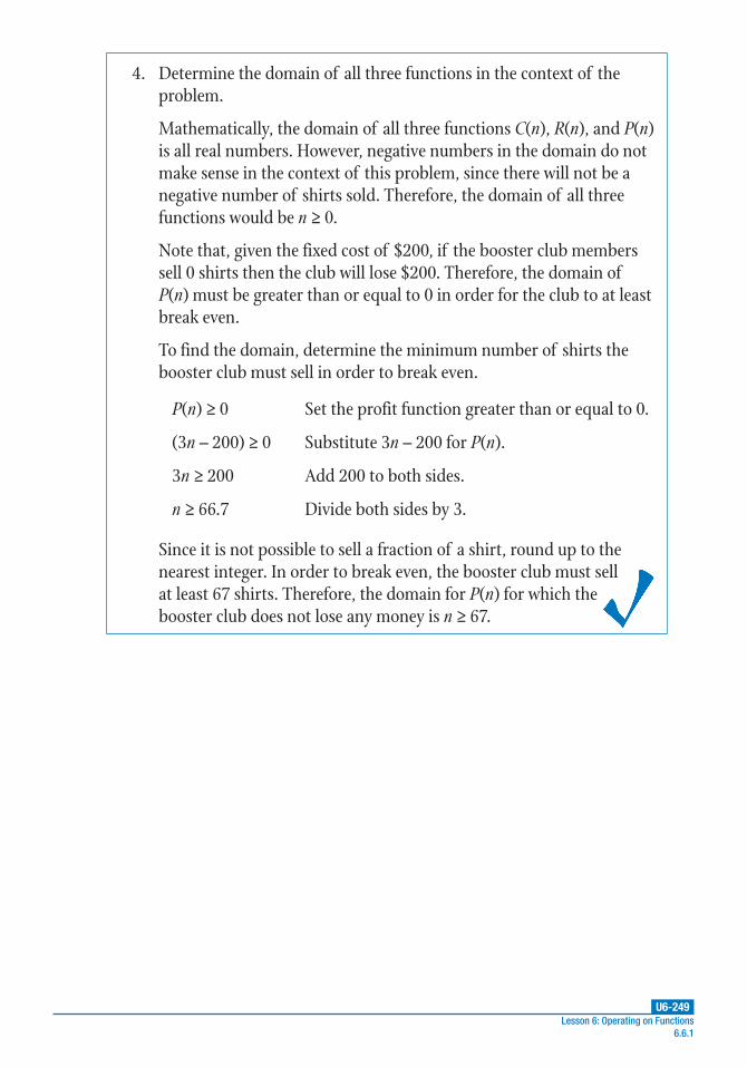
U6-249Lesson 6: Operating on Functions
6.6.1
4. Determine the domain of all three functions in the context of the problem.
Mathematically, the domain of all three functions C(n), R(n), and P(n) is all real numbers. However, negative numbers in the domain do not make sense in the context of this problem, since there will not be a negative number of shirts sold. Therefore, the domain of all three functions would be n ≥ 0.
Note that, given the fixed cost of $200, if the booster club members sell 0 shirts then the club will lose $200. Therefore, the domain of P(n) must be greater than or equal to 0 in order for the club to at least break even.
To find the domain, determine the minimum number of shirts the booster club must sell in order to break even.
P(n) ≥ 0 Set the profit function greater than or equal to 0.
(3n – 200) ≥ 0 Substitute 3n – 200 for P(n).
3n ≥ 200 Add 200 to both sides.
n ≥ 66.7 Divide both sides by 3.
Since it is not possible to sell a fraction of a shirt, round up to the nearest integer. In order to break even, the booster club must sell at least 67 shirts. Therefore, the domain for P(n) for which the booster club does not lose any money is n ≥ 67.

U6-250Unit 6: Mathematical Modeling 6.6.1
Example 3
To increase a basketball team’s fan base, the team’s owners agree to gradually reduce the price of season tickets for games according to the function P(g) = 25 – 0.1g, where P is the price in hundreds of dollars and g is the number of games played so far in the season. Since the beginning of this promotion, the number of fans in attendance, N, has been modeled by the function N(g) = 10 + 0.2g. Create a product function, f(g), from the functions P(g) and N(g). Explain what the product function means in the context of this problem. Graph the product function and use the graph to identify the type of equation and its domain (within the context of the problem).
1. Create a product function f(g) from the functions P(g) and N(g).
To create a product function, multiply P(g) = 25 – 0.1g and N(g) = 10 + 0.2g.
f(g) = P(g) • N(g) Write the functions as a multiplication problem.
f(g) = (25 – 0.1g) • (10 + 0.2g) Substitute 25 – 0.1g for P(g) and 10 + 0.2g for N(g).
f(g) = 250 + 5g – g – 0.02g2 Distribute.
f(g) = –0.02g2 + 4g + 250 Combine like terms.
The product function is f(g) = –0.02g2 + 4g + 250.
2. Explain what the product function means in the context of this problem.
The product function f(g) = –0.02g2 + 4g + 250 represents the revenue from season ticket sales in hundreds of dollars for the number of games played thus far.

U6-251Lesson 6: Operating on Functions
6.6.1
3. Graph the product function and identify its type and domain.
The graph of f(g) = –0.02g2 + 4g + 250 is shown.
–300 –200 –100 100 200 300
x
500
450
400
350
300
250
200
150
100
50
0–50
–100
–150
–200
–250
–300
–350
y
The graph has the shape of a parabola that opens downward. Therefore, f(g) = –0.02g2 + 4g + 250 is a quadratic function.
Mathematically, the domain of the function is all real numbers. However, in the context of this problem, the valid domain must be positive real numbers because the number of games cannot be negative. Therefore, the domain is 0 ≤ x ≤ 250.

U6-252Unit 6: Mathematical Modeling 6.6.1
Example 4
If f(x) = x + 3 and g(x) = –x2 + 4, what types of functions are f(x), g(x), and ( )
( )
f x
g x? What is
the domain of ( )
( )
f x
g x? How does its domain compare with the domains of f(x) and g(x)?
1. Determine the type of each given function.
To determine the type of function, first identify the degree of each function.
The degree of f(x) = x + 3 is 1, so this function is linear.
The degree of g(x) = –x2 + 4 is 2, so this function is quadratic.
The quotient function is ( )
( )
3
42=+
− +f x
g x
x
x. Since there is a variable in
the denominator of 3
42
+− +
x
x,
( )
( )
f x
g x is a rational function.
2. Determine the domain of ( )
( )
f x
g x.
The domain of ( )
( )
f x
g x will be all values except for those that make the
function undefined. Find the values that make the denominator of the
quotient function equal to 0.
–x2 + 4 Denominator of the quotient function
= –1(x2 – 4) Factor out –1.
= –1(x + 2)(x – 2) Factor the polynomial.
Set both factors equal to 0 and solve for x.
x + 2 = 0 x – 2 = 0
x = –2 x = 2
The domain of ( )
( )
f x
g x is all real numbers except for x = 2 and x = –2,
since those values of x make the denominator equal to 0 and thus
make the function undefined.

U6-253Lesson 6: Operating on Functions
6.6.1
3. How does the domain of the quotient function compare with the domains of f(x) and g(x)?
The domain of the quotient function ( )
( )
f x
g x is different from the
domains of the individual functions; the quotient function is
undefined at x = 2 and x = –2, whereas the individual functions
have domains of all real numbers.

U6-254
PRACTICE
UNIT 6 • MATHEMATICAL MODELINGLesson 6: Operating on Functions
Unit 6: Mathematical Modeling 6.6.1
Use what you have learned about operating with functions to complete problems 1 and 2.
1. The value of a collectors-edition DVD boxed set of horror movies was $225 when it first came out. The boxed set has decreased in value at rate of $12.75 per year since. Write an equation, D(t), to represent the average dollar value of the DVD boxed set in terms of years, t.
2. A research study aims to discover a possible link between the number of cell phone users and the number of photo-editing software users in a given year. The number of cell phone users is given by C(x) = 0.8x2 + 5x + 4, and the number of editing software users is given by E(x) = 0.9x, where x is the year of the study. Write an equation for (C + E)(x) and explain its meaning.
Use the following information to complete problems 3–6.
A manufacturer of hair styling tools produces flat irons at a cost of $5.60 per flat iron (x) and a fixed cost of $24,000. Each flat iron sells for $99.50.
3. Write the revenue function, R(x), based on the number of flat irons sold.
4. Write the cost function, C(x), based on the number of flat irons produced.
5. Based on functions R(x) and C(x), what is the profit function, P(x)?
6. Compare the domain of P(x) to the domains of R(x) and C(x).
Practice 6.6.1: Adding, Subtracting, Multiplying, and Dividing Functions
continued

U6-255
PRACTICE
UNIT 6 • MATHEMATICAL MODELINGLesson 6: Operating on Functions
Lesson 6: Operating on Functions 6.6.1
For problems 7 and 8, let P(t) = –9t3 + 5t2 – 18t + 9 represent the retail sales (in billions of dollars) in t years of a particular model of personal watercraft.
7. The function ( )P t represents the average retail sales of the personal watercraft over several years. What is the equation of the average sales function for P(t)?
8. Explain why the domain of the average sales function is t > 0.
The cost to produce a particular toy is modeled by C(x) = 12.30x + 98,000. Use this information to complete problems 9 and 10.
9. What is the equation of the average cost function, C x( ), representing the toy’s costs for multiple years?
10. What types of functions are represented by the cost function and the average cost function?

U6-256Unit 6: Mathematical Modeling 6.6.2
Introduction
The composition of functions is the process of substituting one function for the independent variable of another function to create a new function. The resulting composite function can be used to describe how the change in one quantity (A) affects the change in another quantity (B). In other words, a composition describes what happens when the output of A becomes the input of B. Composite functions can be used to model situations in the real world that describe this phenomenon.
Key Concepts
• A composite function is a function that results from composing two separate functions, f(x) and g(x), so that the output of g(x) is the input of f(x), or vice versa.
• By definition, the composition of two functions f(x) and g(x) can be written as a new function, f(g(x)) or g(f(x)). These notations are read as “f of g of x” and “g of f of x,” respectively.
• f(g(x)) can be written as ( )( )f g x ; either notation means that the function g(x) is substituted for the independent variable x in the function f(x).
• Similarly, g(f(x)), where f(x) is substituted for x in the function g(x), can be written as ( )( )g f x .
• The value of the composite function f(g(x)) is not the same as the value of g(f(x)).
• A composite function can be determined by substituting one function’s formula in place of each “x” in the other function’s formula. For example, let f(x) = x2 and g(x) = 3x. To find f(g(x)), substitute 3x for x in the f(x) function to yield f(3x) = (3x)2, and then simplify. Thus, f(g(x)) = 9x2.
• The domain of a composite function f(g(x)) will be a subset of the domain of the function g(x). Graphically, the domain of the composite function can be determined in terms of coordinates on the graph. Given the point (a, b) in the domain of f(x) and the point (b, c) in the domain of g(x), then the point (a, c) will be in the domain of the composite function, f(g(x)).
• A function can compose with itself, such as f(f(x)), read as “f of f of x.” If f(x) = x + 1, then f(f(x)) = (x + 1) + 1 = x + 2.
Lesson 6.6.2: Composing Functions

U6-257Lesson 6: Operating on Functions
6.6.2
• Graphing calculators can be helpful when graphing composite functions. Use the directions specific to your calculator model to graph composite functions.
On a TI-83/84:
Step 1: Press [Y=].
Step 2: At Y1, enter the first equation, f(x).
Step 3: At Y2, enter the second equation, g(x).
Step 4: At Y3, enter the composite function, ( ( ))=f g f g x , in the form Y1(Y2). Be sure to include the parentheses. Note: To copy the equations for Y1 and Y2 into the Y3 field, press [VARS], then arrow over to Y-Vars. Select 1: Function, and press [ENTER]. In the Function menu, select 1 for Y1. Repeat for each additional function, selecting 2 for Y2, etc.
Step 5: Press [GRAPH]. Press [WINDOW] to adjust the viewing area if necessary.
On a TI-Nspire:
Step 1: Press [home]. Press B to bring up the graphing scratchpad. To clear the scratchpad of any existing equations, press [doc], then arrow down to B: Clear Scratchpad. Press [enter], then use the keypad to select the graphing tab and return to the graphing screen.
Step 2: If no equation entry box (with “f 1(x) =”) is shown, use the touchpad to select the “>>” icon at the bottom left corner of the graphing screen. This will bring up an equation entry box.
Step 3: Type the equation of the first function next to f 1(x). Press [enter].
Step 4: To add the second function, select the “>>” icon to bring up an entry box for f 2(x). Enter the second function at f 2(x) and press [enter].
Step 5: To add the composite function, select the “>>” icon to bring up an entry field for f 3(x). Type the composite equation into the f 3(x) box as f 3(x): = f 1(f 2(x)).
Step 6: If necessary, adjust the viewing area by pressing [menu] and selecting 4: Window/Zoom, then A: Zoom – Fit.

U6-258Unit 6: Mathematical Modeling 6.6.2
Guided Practice 6.6.2Example 1
Given the graphs of f(x) and g(x) as shown, find f(g(1)), g(f(–2)), and f(f(0)).
–5 –4 –3 –2 –1 1 2 3 4 5
x
5
4
3
2
1
0
–1
–2
–3
–4
–5
y
f(x)
–5 –4 –3 –2 –1 1 2 3 4 5
x
5
4
3
2
1
0
–1
–2
–3
–4
–5
y
g(x)
1. Use the graphs to find f(g(1)).
First, determine the value of g(1) using the graph of g(x). Since the graph of g(x) has a point at (1, –1), g(1) = –1.
Next, use this output value of g(1) as the input for f(x). In other words, find f(–1) from the graph of f(x).
Since the graph of f(x) has a point at (–1, –3), f(–1) = –3.
Therefore, the value of f(g(1)) is –3.
2. Use the graphs to find g(f(–2)).
First, determine the value of f(–2) using the graph of f(x). Since the graph of f(x) has a point at (–2, –1), f(–2) = –1.
Next, use this output value of f(–2) as the input for g(x). In other words, find g(–1) from the graph of g(x).
Since the graph of g(x) has a point at (–1, 3), g(–1) = 3.
Therefore, the value of g(f(–2)) is 3.

U6-259Lesson 6: Operating on Functions
6.6.2
3. Use the graphs to find f(f(0)).
First, determine the value of f(0) using the graph of f(x). Since the graph of f(x) has a point at (0, –2), f(0) = –2.
Next, use this output value of f(0) as the input for f(x). In other words, find f(–2) from the graph of f(x).
Since the graph of f(x) has a point at (–2, –1), f(–2) = –1.
Therefore, the value of f(f(0)) is –1.
Example 2
Let f(x) = 2x + 3 and ( )5 1
2 3=
+−
g xx
x. Find f(g(x)) and g(f(x)), and determine whether the
two composite functions are equal.
1. Find f(g(x)).
Use the given functions to write a function for f(g(x)). The output
of g(x) is being used as the input for f(x); therefore, in f(x), substitute 5 1
2 3
+−
x
x for x and simplify.
f(x) = 2x + 3 Original function for f(x)
( ( )) 25 1
2 33=
+−
+f g x
x
xSubstitute
5 1
2 3
+−
x
x for x and
rename f(x) as f(g(x)).
( ( ))10 2
2 33=
+−
+f g xx
xDistribute.
Therefore, ( ( ))10 2
2 33=
+−
+f g xx
x.

U6-260Unit 6: Mathematical Modeling 6.6.2
2. Find g(f(x)).
Use the given functions to write a function for g(f(x)). The output of f(x) is being used as the input for g(x); therefore, in g(x), substitute 2x + 3 for x and simplify.
( )5 1
2 3=
+−
g xx
x Original function for g(x)
( ( ))5(2 3) 1
2(2 3) 3=
+ ++ −
g f xx
x
Substitute 2x + 3 for x and rename g(x) as g(f(x)).
( ( ))10 15 1
4 6 3=
+ ++ −
g f xx
xDistribute.
( ( ))10 16
4 3=
++
g f xx
xSimplify.
Therefore, ( ( ))10 16
4 3=
++
g f xx
x.
3. Determine whether f(g(x)) and g(f(x)) are equal.
The composite functions are ( ( ))10 2
2 33=
+−
+f g xx
x and
( ( ))10 16
4 3=
++
g f xx
x. Since
10 2
2 33
10 16
4 3
+−
+ ≠++
x
x
x
x, g(f(x)) is not
equal to f(g(x)).

U6-261Lesson 6: Operating on Functions
6.6.2
Example 3
Given h(x) = 3x + 12 and k(x) = x, determine the equation of the composite function k(h(x)), graph the composite function, and then determine its domain.
1. Determine the equation of the composite function k(h(x)).
The output of h(x) is being used as the input for k(x); therefore, substitute 3x + 12 for x in the function k(x).
k(x) = x Original function for k(x)
k(h(x)) = (3x + 12) Substitute 3x + 12 for x and rename k(x) as k(h(x)).
The equation of the composite function is k(h(x)) = 3x + 12.
2. Graph the composite function by hand or using a graphing calculator.
The graph of k(h(x)) = 3x + 12 is shown.
–10 –8 –6 –4 –2 2 4 6 8 10
x
10
8
6
4
2
0
–2
–4
–6
–8
–10
y
3. Determine the domain of the composite function.
k(h(x)) = 3x + 12 is defined at all values of x, so the domain is all real numbers.

U6-262Unit 6: Mathematical Modeling 6.6.2
Example 4
The number of old-fashioned rocking chairs, n, sold at a furniture store is a function
of the price of each chair, p, as modeled by ( )5(360 )
80=
−−
n pp
p for p > 80. The cost to
the store, c, in dollars for each chair is a function of the number of chairs, n, that the
store sells each week, and is modeled by c(n) = 0.002(n + 2)2 + 80. Express the cost of
each chair as a function of the selling price if c(p) = c(n(p)), and determine the type of
function created by this composition. What is the cost of each chair if the selling price
is $120? What would the profit per chair be at that selling price?
1. Express the cost of each chair as a function of the selling price, and determine the type of function.
Find c(p) given n(p) and c(n). Since c(p) = c(n(p)), this means that the
output of n(p) is being used as the input of c(n). Therefore, substitute 5(360 )
80
−−
p
p for the variable n in c(n).
c(n) = 0.002(n + 2)2 + 80 Original function for c(n)
( ) 0.0025(360 )
802 80
2
=−
−
+
+c p
p
p
Substitute 5(360 )
80
−−
p
p for
n and rename c(n) as c(p).
( ) 0.0021800 5
802 80
2
=−
−
+
+c p
p
p
Distribute the numerator inside the parentheses.
The cost of each chair as a function of the selling price can be
expressed as ( ) 0.0021800 5
802 80
2
=−
−
+
+c p
p
p, which is a rational
function because there is a variable in the denominator.
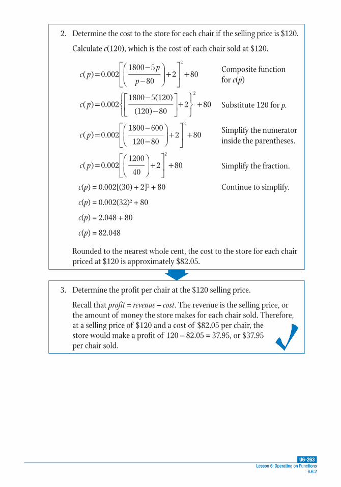
U6-263Lesson 6: Operating on Functions
6.6.2
2. Determine the cost to the store for each chair if the selling price is $120.
Calculate c(120), which is the cost of each chair sold at $120.
( ) 0.0021800 5
802 80
2
=−
−
+
+c p
p
pComposite function for c(p)
( ) 0.0021800 5(120)
(120) 802 80
2
=−−
+
+c p Substitute 120 for p.
( ) 0.0021800 600
120 802 80
2
=−−
+
+c p Simplify the numerator
inside the parentheses.
( ) 0.0021200
402 80
2
=
+
+c p Simplify the fraction.
c(p) = 0.002[(30) + 2]2 + 80 Continue to simplify.
c(p) = 0.002(32)2 + 80
c(p) = 2.048 + 80
c(p) = 82.048
Rounded to the nearest whole cent, the cost to the store for each chair priced at $120 is approximately $82.05.
3. Determine the profit per chair at the $120 selling price.
Recall that profit = revenue – cost. The revenue is the selling price, or the amount of money the store makes for each chair sold. Therefore, at a selling price of $120 and a cost of $82.05 per chair, the store would make a profit of 120 – 82.05 = 37.95, or $37.95 per chair sold.

U6-264
PRACTICE
UNIT 6 • MATHEMATICAL MODELINGLesson 6: Operating on Functions
Unit 6: Mathematical Modeling 6.6.2
Use the following information to complete problems 1 and 2.
A pebble dropped in a still pond causes ripples of circles. The radius in feet of the largest circle is r(t) = 0.6t, where t is the time in seconds after the pebble hits the water.
1. Given that the area of a circle is A(r) = πr2, find A(r(t)).
2. What does the composite function mean in this context?
Use the following information to complete problems 3–7.
C(x) = 60x + 750 represents the weekly cost of producing x units in a manufacturing process. The number of units P produced in t hours is P(t) = 50t.
3. What is C(P(t))?
4. Interpret the meaning of C(P(t)) in the context of the problem.
5. Find P(C(x)).
6. Interpret the meaning of P(C(x)) in the context of the problem.
7. Which composite function would you use to find the number of units produced in 4 hours? How many units are produced?
Practice 6.6.2: Composing Functions
continued

U6-265
PRACTICE
UNIT 6 • MATHEMATICAL MODELINGLesson 6: Operating on Functions
Lesson 6: Operating on Functions 6.6.2
Use the following information to complete problem 8.
The oldest of three siblings is twice the age of the middle one. The age of the youngest is twice the middle sibling’s age less six years.
8. Write a composite function, A, that gives the oldest sibling’s age in terms of the youngest one’s age. Use m for the age (in years) of the middle sibling.
Use the following information to complete problems 9 and 10.
The temperature of food in a freezer is given by N(T) = 10T 2 – 20T + 600, where T is the temperature in degrees Celsius. When the food is moved from the freezer to the refrigerator to thaw, its temperature can be given by P(t) = 2t + 1, with t representing the time in hours.
9. Find N(P(t)).
10. Interpret the meaning of N(P(t)) in the context of the problem.

Lesson 7: Inverses of FunctionsUNIT 6 • MATHEMATICAL MODELING
U6-266Unit 6: Mathematical Modeling 6.7
Common Core Georgia Performance Standards
MCC9–12.F.BF.4a
MCC9–12.F.BF.4b (+)
MCC9–12.F.BF.4c (+)
Essential Questions
1. How can you determine if the functions f(x) and g(x) are inverse functions of each other if f(a) = b and g(b) = a?
2. How do the graphs of a function f(x) and its inverse f –1(x) compare?
3. How do the domains and ranges of a function and its inverse compare?
4. How can you identify a function that does not have an inverse?
WORDS TO KNOW
axis of symmetry a line that divides a figure into symmetric parts
composition of functions the process of substituting one function for the independent variable of another function to create a new function
domain the set of all input values (x-values) that satisfy the given function without restriction
function a relation in which every element of the domain is paired with exactly one element of the range; that is, for every value of x, there is exactly one value of y
inverse function the function that results from switching the x- and y-variables in a given function; the inverse of f(x) is written as f –1(x)
inverse relation a relation g(x) such that g(f(x)) = x and f(g(y)) = y where f(x) is a function

U6-267Lesson 7: Inverses of Functions
6.7
one-to-one correspondence
the feature of a function whereby each value in the domain corresponds to a unique function value; that is, if x = a and x = b, the two points would be (a, f(a)) and (b, f(b)), and if a ≠ b, then f(a) ≠ f(b) for a function to exhibit one-to-one correspondence
quadratic function a function defined by a second-degree expression of the form f(x) = ax2 + bx + c, where a ≠ 0 and a, b, and c are constants. The graph of any quadratic function is a parabola.
range the set of all outputs of a function; the set of y-values that are valid for the function
relation a relationship between two variables in which at least one value of the domain or independent variable, x, is matched with one or more values of the dependent or range variable, y
restricted domain a subset of a function’s defined domain
symmetrical having two parts that are mirror images when reflected over a line or rotated around a point
symmetry of a function the property whereby a function exhibits the same behavior (e.g., graph shape, function values) for specific domain values and their opposites
U6-268Unit 6: Mathematical Modeling 6.7
Recommended Resources
• Analyzemath.com. “Inverse of Quadratic Functions.”
http://www.walch.com/rr/00227
This site provides easy-to-follow, simple examples of how to find the inverse of a quadratic function with a restricted domain. Note: The shorthand “sqrt(x)” is used for x .
• ChiliMath. “Finding the Inverse Function of a Quadratic Function.”
http://www.walch.com/rr/00228
This tutorial covers how to quickly determine whether a quadratic function has an inverse, and if so, how to find the inverse. Example problems work through the solutions step-by-step.
• MathIsFun.com. “Inverse Functions.”
http://www.walch.com/rr/00229
This site uses a step-by-step approach to explain and review inverse functions.
• Purplemath.com. “Inverse Functions: Definition of ‘Inverse’ / Drawing the Inverse from a Graph.”
http://www.walch.com/rr/00276
This site describes techniques for using the graph of a function to find its inverse. The examples give insight into what the inverse of a function means visually by examining specific points on a graph.
U6-269Lesson 7: Inverses of Functions
6.7.1
Introduction
Several kinds of relationships exist between variables. For example, a relation is a relationship between two variables in which at least one value of the domain or independent variable, x, is matched with one or more values of the dependent or range variable, y. The domain refers to the set of all input values (x-values) that satisfy the given function without restriction and the range refers to the values of the dependent variable of the function. Sometimes, a relation is said to be a function, a relation in which every element of the domain is paired with exactly one element of the range; that is, for every value of x, there is exactly one value of y. Both relations and functions have inverses. In this section, we will explore how to determine the inverse of a quadratic function, as well as how to verify where the inverse exists.
Key Concepts
• Determining the inverse of a function often requires examining the original function’s domain and range.
• An inverse relation is a relation g(x) such that g(f (x)) = x and f ( g ( y)) = y where f (x) is a function.
• If the inverse relation g(x) is also a function, it is said to be an inverse function. It is the function that results from switching the x- and y-variables in the given function, f(x). The inverse of f(x) is also written as f –1(x).
• Note that this f –1(x) notation does not mean to take the –1 power of f(x). Both notations, f –1(x) and g(x), are used to represent an inverse.
• A function g(x) is the inverse of a function f(x) if g( f (x)) = x and f ( g( y)) = y; or, g(x) is the inverse of f(x) if f(a) = b and g(b) = a.
• For example, if f(x) = x + 1, then we can switch the domain and range variables (x and f(x)) and rename f(x) as g(x) to arrive at its inverse: the inverse of f(x) = x + 1 is x = g(x) + 1. Or, solved for g(x), g(x) = x – 1. Notice that f(x) becomes its inverse g(x) once the variables are switched.
Lesson 6.7.1: Finding and Graphing Inverses of Functions

U6-270Unit 6: Mathematical Modeling 6.7.1
• For a function to have an inverse function, it has to satisfy the condition of one-to-one correspondence. This means that each value in the domain corresponds to a unique function value; that is, if x = a and x = b, the two points would be (a, f(a)) and (b, f(b)); if a ≠ b, then f(a) ≠ f(b) for a function to exhibit one-to-one correspondence. In other words, for a function to have an inverse, it cannot have the same range/output value for two different domain values. It is particularly important to check for one-to-one correspondence when finding the inverse of a quadratic function.
• Recall that a quadratic function is a second-degree function of the form f(x) = ax2 + bx + c, where a ≠ 0 and a, b, and c are constants. The graph of any quadratic function is a parabola.
• Since quadratic functions are parabolic, this means there is likely more than one output value for each input value, or more than one input value for each output, depending on the equation. For example, if f(x) = x2, then values of x = 2 and x = –2 both result in f(x) = 4. The resulting points, (2, 4) and (–2, 4), do not have unique output values—they share 4 as the output. Therefore, determining the inverse of a quadratic function requires some additional steps.
• To construct an inverse relation or a possible inverse function for a quadratic function, switch the dependent and independent variables, x and y, and solve for the new function, y.
• For example, take the function f(x) = 3x2 – 4. Switching the variables and
renaming f(x) as g(x) results in x = 3[g(x)]2 – 4. Simplifying and solving this new
equation for g(x) results in g xx3( 4)
3( )= ±
+.
• A restricted domain is a subset of a function’s defined domain. The subset is limited by mathematical conditions and/or real-world constraints.
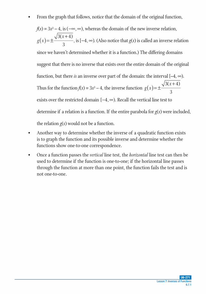
U6-271Lesson 7: Inverses of Functions
6.7.1
• From the graph that follows, notice that the domain of the original function,
f(x) = 3x2 – 4, is ( , )−∞ ∞ , whereas the domain of the new inverse relation,
g xx3( 4)
3( )= ±
+, is [ 4, )− ∞ . (Also notice that g(x) is called an inverse relation
since we haven’t determined whether it is a function.) The differing domains
suggest that there is no inverse that exists over the entire domain of the original
function, but there is an inverse over part of the domain: the interval [–4, ∞).
Thus for the function f(x) = 3x2 – 4, the inverse function g xx3( 4)
3( )= ±
+
exists over the restricted domain [ 4, )− ∞ . Recall the vertical line test to
determine if a relation is a function. If the entire parabola for g(x) were included,
the relation g(x) would not be a function.
• Another way to determine whether the inverse of a quadratic function exists is to graph the function and its possible inverse and determine whether the functions show one-to-one correspondence.
• Once a function passes the vertical line test, the horizontal line test can then be used to determine if the function is one-to-one; if the horizontal line passes through the function at more than one point, the function fails the test and is not one-to-one.

U6-272Unit 6: Mathematical Modeling 6.7.1
• To visualize this, look at the graph of f(x) = 3x2 – 4 and its positive inverse,
g xx3( 4)
3.( )=
+ (Note that the negative inverse, g x
x3( 4)
3( )= −
+, has
been excluded from the graph.) A horizontal line has been drawn through the
graph of f(x) at y = 1.5.
–10 –8 –6 –4 –2 20 4 6 8 10
x
10
8
6
4
2
–2
–4
–6
–8
–10
y
f(x)
g(x)y = 1.5
• Notice that the horizontal line y = 1.5 intersects the original function at two points, which means that f(x) = 3x2 – 4 does not have an inverse over its entire domain of ( , )−∞ ∞ . In other words, there is not one-to-one correspondence for each point on f(x): the function values of f(x) have two possible domain values over some parts of the domain.
• However, if the domain is restricted to the intervals [0, )∞ or [–4, 0], then f(x) does have an inverse g(x) because the domain of g(x), [ 4, )− ∞ , includes the restricted domains. Thus, it is possible for a quadratic function to have an inverse, given a restricted domain.
• A graphing calculator can be used to explore a quadratic function and the domain(s) over which its inverse exists.

U6-273Lesson 7: Inverses of Functions
6.7.1
• Note that a graphing calculator will not provide rigorous proof of the existence of an inverse and its domain. Furthermore, the horizontal line test is not as accurate a method of testing a function and its inverse for one-to-one correspondence. Therefore, when using a graphing calculator, it is necessary to check the results algebraically after plotting the functions.
On a TI-83/84:
Step 1: Press [Y=]. Press [CLEAR] to delete any other functions stored on the screen.
Step 2: At Y1, enter the original function using your keypad. Press [ENTER].
Step 3: Enter the possible inverse function(s) using your keypad. Note:
When both positive and negative inverses are possible, each
function needs to be entered separately to be graphed. For example,
to graph g xx3( 4)
3( )= ±
+, enter
x3( 4)
3
+ at Y2 and
x3( 4)
3−
+
at Y3. Press [ENTER].
Step 4: To view a graph of f (x) and its inverse g(x), press [GRAPH].
Step 5: To view the table of values, press [2ND][GRAPH]. Take note of any undefined values for the functions.

U6-274Unit 6: Mathematical Modeling 6.7.1
On a TI-Nspire:
Step 1: Press the [home] key.
Step 2: Arrow over to the graphing icon, the second icon from the left, and press [enter].
Step 3: At f 1(x), enter the original function using your keypad. Press [enter].
Step 4: To enter the possible inverse function(s), press [tab]. Note: When
both positive and negative inverses are possible, each function
needs to be entered separately to be graphed. For example, to graph
g xx3( 4)
3( )= ±
+, enter
x3( 4)
3
+ at f 2(x) and
x3( 4)
3−
+ at
f 3(x). Press [enter].
Step 5: To view the graphs of f (x) and its inverse g(x), press [tab]. Arrow up to display the equation you wish to graph, and then press [enter]. Repeat for each equation you wish to graph on the same screen.
Step 6: To view the table of values, press [ctrl][T]. Take note of any undefined values for the functions.
• Finding the inverse of functions that are not quadratic—such as radical, rational, and cubic functions—is similar to the process for finding the inverse of a quadratic function.
• For example, take the rational function ( )5
1f x
x=
−. Switching the variables
and rewriting with f –1(x) in place of f(x) yields the equation 5
( ) 11xf x
=−− .
• Remember: f –1(x) notation does not mean to take the –1 power of f(x).
• As with quadratic functions, this equation needs to be simplified and solved
algebraically for f –1(x). The resulting equation, ( )5
1f xx
x=
+− , is the possible
inverse of the original function.

U6-275Lesson 7: Inverses of Functions
6.7.1
• Does the possible inverse of the function exist? To visualize this, compare the graphs of the two functions.
–10 –8 –6 –4 –2 20 4 6 8 10x
10
8
6
4
2
–2
–4
–6
–8
–10
y
f(x)
f –1(x)
f –1(x)
f(x)
• Notice that the domain of the original function is ( ,1) (1, )−∞ ∩ +∞ , whereas the domain of the inverse is ( ,0) (0, )−∞ ∩ +∞ . From the graph of the function, it can be seen that the x-values of the domain of the original function extend from negative infinity to 1 and from 1 to positive infinity. This excludes 1 from the domain of the original function. The domain of the inverse extends from negative infinity to 0 and from 0 to positive infinity. The domain of the inverse excludes 0.
• Examine the graph of the function and its inverse and use the horizontal line test. It can be seen that for the function and its inverse, each value in the domain corresponds to a unique function value. Therefore, the function and its inverse exhibit one-to-one correspondence. The original function approaches the horizontal asymptote y = 0 as x approaches ±∞ , and the inverse approaches the horizontal asymptote y = 1 as x approaches ±∞ .
• To find the domain over which both a function and its inverse exist, look at the individual domains of each and where they are defined. In this example, the combined domain is ( ,0) (0,1) (1, )−∞ ∩ ∩ +∞ because the function and the inverse have different domain values at which they are undefined.
• As with quadratic functions and their inverses, a graphing calculator can be used to explore a function and the domain(s) over which its inverse exists. Refer to the instructions provided on the previous pages.

U6-276Unit 6: Mathematical Modeling 6.7.1
Guided Practice 6.7.1Example 1
Find the inverse, g(x), of the function f(x) = 4x2 and determine the domain value(s) over which the inverse exists.
1. Switch the domain and function variables, and then rename f(x) as g(x).
Since the inverse function results from switching the input and output variables of the original function, identify which variable represents the input and which represents the output. For the function f(x) = 4x2, x is the input (independent) variable, and f(x) is the output (dependent) variable. Therefore, swap f(x) and x.
f(x) = 4x2 Original function
x = 4[f(x)]2 Switch f(x) and x.
Next, rename f(x) as g(x), since this new relation represents the inverse of the original function.
x = 4[f(x)]2 Equation with variables switched
x = 4[g(x)]2 Rename f(x) as g(x).
The resulting inverse relation, x = 4[g(x)]2, is the possible inverse function of the original function. It must be evaluated to determine whether it has one-to-one correspondence with the original function, f(x) = 4x2.

U6-277Lesson 7: Inverses of Functions
6.7.1
2. Solve the possible inverse for g(x).
x = 4[g(x)]2 Possible inversex
g x4
[ ( )]2= Divide both sides by 4.
g xx
( )4
2 = Rearrange using the Symmetric Property of Equality.
g xx
( )4
= ± Take the square root of both sides.
g xx
( )4
= ±Apply the square root to both the numerator and the denominator.
g xx
( )2
= ± Simplify.
g x x( )1
2= ± Eliminate the denominator by rewriting the
division as multiplication by a fraction.
3. Determine the domain of g(x).
We need to know where g(x) is defined in order to know its domain, which we want to compare to the range of f(x).
g(x) is a radical function; specifically, it is a square root function. Recall that the value of the expression inside the radical must be positive in order for the function to be defined. The expression under the square root is x; therefore, the values of x are limited to non-negative numbers.
Thus, the domain of g(x) is [0, )+∞ because x is raised to the 1
2 power (recall that x x
1
2= ).

U6-278Unit 6: Mathematical Modeling 6.7.1
4. Determine the range of g(x).
We need to compare the range of g(x) to the domain of f(x).
There are no limitations on the output values; therefore, the range of g(x) is ( , ).−∞ +∞
5. Determine the domain of f(x).
The domain of f(x) is ( , ).−∞ +∞ The domain will need to be restricted to those values over which f(x) shows one-to-one correspondence.
6. Determine whether the function f(x) exhibits one-to-one correspondence.
The function f(x) can only have an inverse over the part of its domain for which it exhibits one-to-one correspondence.
We can determine that the function f(x) = 4x2 does not show one-to-one correspondence for all range values because x = a and x = –a yield equal values for f(x): f(a) = 4a2 and f(–a) = 4(–a)2 = 4a2. You can apply the horizontal line test and exclude portions of f(x) where this test fails; that is, where the horizontal line crosses f(x) at more than one point.
7. Determine the parts of its domain over which f(x) exhibits one-to-one correspondence.
The restricted domains of f(x) are ( , 0]−∞ and [0, ).+∞ Only the point (0, 0) is not restricted, because all of the other points do not have one-to-one correspondence. The horizontal line crosses the graph at two points for all other points on the graph.
8. Determine the range of f(x).
Because f(x) is a quadratic function and x2 can never be negative, the range of f(x) is [0, )+∞ .

U6-279Lesson 7: Inverses of Functions
6.7.1
9. Match domains to ranges to find the inverse(s) of f(x).
In order for a function to have an inverse, it must be one-to-one. Therefore, match the restricted domains of f(x) to the range of g(x).
Restricted domain of f(x): Inverse function with matching range:
[0, )+∞ =g x x( )1
2
( , 0]−∞ =−g x x( )1
2
Check that the range of f(x) matches the domain of g(x).
The range of f(x) is [0, )+∞ . The domain of g(x) is [0, )+∞ .
The inverse of f(x) = 4x2 on the restricted domain ≤ <+∞0 x is
=g x x( )1
2.
The inverse of f(x) = 4x2 on the restricted domain −∞< ≤0x is
=−g x x( )1
2.
U6-280Unit 6: Mathematical Modeling 6.7.1
Example 2
Find the inverse of the function ( )1
f xx
x=
− if it exists, and determine the domain
value(s) shared by the inverse and the function.
1. Switch the domain and function variables, and then rewrite using inverse function notation.
Switch f(x) and x; then, replace f(x) with f –1(x).
( )1
f xx
x=
−Original function
xf x
f x
( )
( ) 1[ ]=− Switch the variables.
( )
( ) 1
1
1x
f x
f x= −
−
− Rewrite using f –1(x) notation.
The resulting relation, ( )
( ) 1
1
1x
f x
f x= −
−
− , is the possible inverse of the
original function. It must be evaluated to determine whether it has
one-to-one correspondence with the original function.

U6-281Lesson 7: Inverses of Functions
6.7.1
2. Solve the possible inverse for f –1(x).
( )
( ) 1
1
1x
f x
f x= −
−
− Possible inverse
x f x f x( ) 1 ( )1 1{ }• − =− −Multiply both sides of the equation by ( ) 11f x −
− .
( ) ( )1 1x f x x f x − =− − Distribute.
( ) ( )1 1x f x f x x = +− − Add x to both sides of the equation.
( ) ( )1 1x f x f x x − =− − Subtract f –1(x) from both sides of the equation.
( ) ( 1)1f x x x − =− Factor out f –1(x) from the left side of the equation.
( )1
1f xx
x=
−− Divide both sides of the
equation by x – 1.
3. Determine the domain of f –1(x).
The domain will be needed in order to define where f –1(x) exists in comparison to f(x). The domain of f –1(x) is ( ,1) (1, )−∞ ∩ +∞ because f –1(x) is undefined at x = 1. Therefore, the domain is all real numbers except x = 1.
4. Determine the range of f –1(x).
The range of f –1(x) is also ( ,1) (1, )−∞ ∩ +∞ since f –1(x) has a horizontal asymptote at y = 1. Therefore, the range is all real numbers except y = 1.

U6-282Unit 6: Mathematical Modeling 6.7.1
5. Determine whether the function f(x) exhibits one-to-one correspondence.
The function can only have an inverse over the part of its domain for which it exhibits one-to-one correspondence.
Let x = a be a possible domain value of the function so that
( )1
f aa
a=
−. Then, let x = –a and evaluate the function:
( )1 1
f aa
a
a
a− =
−− −
=+
.
Since f(a) ≠ f(–a), this means that different function values result for the domain values x = a and x = –a ; therefore, f(x) shows one-to-one correspondence.
This can also be seen on the graphing calculator. Follow the steps appropriate to your calculator model to view the function and its inverse.
On a TI-83/84:
Step 1: Press [Y=]. Press [CLEAR] to delete any other functions stored on the screen.
Step 2: Enter the original function on the Y1 line.
Step 3: Press [GRAPH] to see a graph of f(x). For better viewing, adjust the domain and function variables by pressing [WINDOW] and changing the values.
Step 4: To view a table of domain and function values, press [2ND][GRAPH]. This shows that this function exhibits one-to-one correspondence.
Step 5: To see a graph of the inverse of f(x), press [2ND][PRGM] to display the DRAW menu. Select 8: DrawInv.
Step 6: After “DrawInv” and the cursor appear on the screen, press [VARS]. Arrow over to Y-VARS and select 1: Function.
Step 7: Highlight 1: Y1 and press [ENTER]. This will display “DrawInv Y1.” Press [ENTER] to graph the inverse of the function entered as Y1.
(continued)

U6-283Lesson 7: Inverses of Functions
6.7.1
On a TI-Nspire:
Step 1: Press [home].
Step 2: Arrow over to the graphing icon, the second icon from the left, and press [enter].
Step 3: At f 1(x), enter the original function. Press [enter].
Step 4: Press [tab], and then enter the inverse function at f 2(x). Press [enter].
–10 –8 –6 –4 –2 20 4 6 8 10
x
10
8
6
4
2
–2
–4
–6
–8
–10
y
= −f xx
x( ) 1
= −−f x
xx( ) 1
1
Either calculator will show that the graphs of f (x) and f –1(x) are the same graph.
6. Compare the domains of the function and its inverse to determine where f(x) has an inverse, f –1(x).
Both the function and its inverse have a domain of ( ,1) (1, )−∞ ∩ +∞ . (Note: This is a situation in which a function and its inverse have identical equations.)

U6-284Unit 6: Mathematical Modeling 6.7.1
Example 3
Find the inverse of the radical function ( ) 23f x x= + if it exists, and determine the domain over which the function and its inverse exist.
1. Switch the domain and function variables, and then rewrite using inverse function notation.
This is the first step in determining if the function has an inverse.
Switch f(x) and x; then, replace f(x) with f –1(x).
( ) 23f x x= + Original function
( ) 23x f x[ ]= + Switch the variables.
( ) 213x f x= +− Rewrite using f –1(x) notation.
Next, solve for f –1(x).
( ) 213x f x= +− Possible inverse
( ) 23 1x f x= +− Cube both sides of the equation.
2 ( )3 1x f x− = − Subtract 2 from both sides of the equation.
( ) 21 3f x x= −− Apply the Symmetric Property of Equality.
The possible inverse of ( ) 23f x x= + is f –1(x) = x3 – 2.
2. Determine the domain of the function and the domain of the inverse.
The domain of both the function and its inverse is ( , )−∞ +∞ since nonzero cube roots can be positive or negative.

U6-285Lesson 7: Inverses of Functions
6.7.1
3. Determine whether the function f(x) exhibits one-to-one correspondence with its inverse.
To do this, graph the function and the possible inverse relation. From the graph, visually determine if the possible inverse relation is a function by applying the vertical line test. If both the function and its possible inverse relation pass the horizontal line test, then they have one-to-one correspondence.
Follow the directions appropriate to your calculator model.
On a TI-83/84:
Step 1: Press [Y=]. Press [CLEAR] to delete any other functions stored on the screen.
Step 2: Enter the original function on the Y1 line.
Step 3: Press [GRAPH] to see a graph of f(x). For better viewing, adjust the domain and function variables by pressing [WINDOW] and changing the values.
Step 4: To view a table of domain and function values, press [2ND][GRAPH]. This shows that the function exhibits one-to-one correspondence.
Step 5: To see a graph of the inverse of f(x), press [2ND][PRGM] to display the DRAW menu. Select 8: DrawInv.
Step 6: After “DrawInv” and the cursor appear on the screen, press [VARS]. Arrow over to Y-VARS and select 1: Function.
Step 7: Highlight 1: Y1 and press [ENTER]. This will display “DrawInv Y1.” Press [ENTER] to graph the inverse of the function entered as Y1.
On a TI-Nspire:
Step 1: Press [home].
Step 2: Arrow over to the graphing icon, the second icon from the left, and press [enter].
Step 3: At f 1(x), enter the original function. Press [enter].(continued)

U6-286Unit 6: Mathematical Modeling 6.7.1
Step 4: Press [tab], and then enter the inverse function at f 2(x). Press [enter].
– 10 – 8 – 6 – 4 – 2 20 4 6 8 10
x
10
8
6
4
2
– 2
– 4
– 6
– 8
– 10
y
f(x)
y = x
f –1(x)
As both graphing calculators show, the function and its inverse are one-to-one over the domain ( , )−∞ +∞ .

U6-287Lesson 7: Inverses of Functions
6.7.1
Example 4
Find the inverse of the absolute-value function f x x( ) 2= + if it exists, and determine the domain and range of the inverse.
1. Write the inverse of the function and simplify it.
Switch f(x) and x; then, replace f(x) with f –1(x).
f x x( ) 2= + Original function
( ) 2x f x[ ]= + Switch the variables.
( ) 21x f x= +− Rewrite using f –1(x) notation.
The absolute-value notation implies that x = f –1(x) + 2 or x = –[f –1(x) + 2]. Simplify and solve each of these equations for f –1(x).
x = f –1(x) + 2 x = –[f –1(x) + 2]
x – 2 = f –1(x) x = –f –1(x) – 2
f –1(x) = x – 2 f –1(x) = –x – 2
The possible inverse can be written as f –1(x) = x – 2 or –x – 2.
2. Graph the function and its inverse on a graphing calculator.
On a TI-83/84:
Step 1: Press [Y=]. Press [CLEAR] to delete any other functions stored on the screen.
Step 2: Enter the function on the Y1 line. To enter the absolute value function, select [2ND][CATALOG] and choose “abs(”. Press [ENTER].
Step 3: Enter the possible inverse functions at Y2 and Y3. Press [ENTER].
Step 4: To see the graphs of the functions, press [GRAPH].
(continued)

U6-288Unit 6: Mathematical Modeling 6.7.1
On a TI-Nspire:
Step 1: Press the [home] key.
Step 2: Arrow over to the graphing icon, the second icon from the left, and press [enter].
Step 3: At f1(x), enter the original function. To enter the absolute value symbol, press [ctrl][×] to open the math expressions palette, then select the absolute value symbol. Press [enter].
Step 4: Press [tab] to enter the possible inverse function at f2(x) and f3(x). Press [enter]. The graphs will be displayed.
The resulting graph should resemble the following.
–10 –8 –6 –4 –2 20 4 6 8 10
x
10
8
6
4
2
–2
–4
–6
–8
–10
y
( ) 2f x x= + ( ) 21f x x –−
( ) 21f x x –− –
3. Determine the domain and range of the function.
The minimum point on the graph of the function occurs when x 2 0+ = , which can be represented by the two equalities x + 2 = 0
and –(x + 2) = 0. The solution to these equations is x = –2. Therefore, the domain of the function is ( , )−∞ +∞ . The range of the function is [0, )+∞ since its minimum value is 0, which occurs at x = –2.

U6-289Lesson 7: Inverses of Functions
6.7.1
Example 5
Graph the cubic function f(x) = x3 – 4x2 + 3x and determine the restricted domain(s) over which its inverse exists.
1. Graph the function using a graphing calculator.
This is the quickest way to see the function’s domain and to specify the restricted domain(s) over which it has an inverse.
Follow the directions appropriate to your calculator model.
On a TI-83/84:
Step 1: Press [Y=]. Press [CLEAR] to delete any other functions stored on the screen.
Step 2: Enter the function on the Y1 line. Press [GRAPH].
On a TI-Nspire:
Step 1: Press the [home] key.
Step 2: Arrow over to the graphing icon, the second icon from the left, and press [enter].
Step 3: At f1(x), enter the original function. Press [enter].
Keep this view on the calculator for reference in the next example step.
4. Identify the restricted domain(s) over which the function can have an inverse.
The graph shows that the function is not one-to-one over its domain, but it is one-to-one over the restricted domains of ( , 2]−∞ − and [ 2, )− +∞ . Note that the function can be divided at the point (–2, 0). Therefore, restricted values of the domain are ( , 2]−∞ − and [ 2, )− +∞ .
5. Find the domain and range of the inverse.
The inverse can be represented by = −− ( ) 21f x x and =− −− ( ) 21f x x .
The domain of the inverse is the range of the function. Therefore, the domain of the inverse is [0, )+∞ .
The range of the inverse is the domain of the function. Therefore, the range of the inverse is ( , 2]−∞ − and [ 2, )− +∞ .

U6-290Unit 6: Mathematical Modeling 6.7.1
2. Identify the restricted domain(s) over which the function is not one-to-one.
This can be approximated visually, but the graphing calculator’s trace features will give a more precise result.
A visual approximation suggests that the restricted domain over which the function is not one-to-one is from x ≈ 0.5 to x ≈ 3. This is the portion of the graph that does not pass the horizontal line test.
Confirm this using the method appropriate to your calculator model.
On a TI-83/84:
Step 3: Press [TRACE].
Step 4: Use the left and right arrow keys to move the cursor to the left local maximum at about x = 0.5. Notice that the function has a maximum value at the point (0.42553192, 0.62934032).
Step 5: Move the cursor to the right to the point at which the function has approximately the same value as in the previous step, which is (3.0851064, 0.54747021).
On a TI-Nspire:
Step 4: Press [menu]. Select 5: Trace, and then select 1: Graph Trace.
Step 5: Move the cursor to the left local maximum at about x = 0.5. Notice that at exactly the maximum function value, “maximum” appears. This point should be (0.45, 0.63).
Step 6: Move the cursor right to the point on the curve that is at approximately the same function value as the maximum found in the previous step. (This may require changing the trace settings: press [menu], select 5: Trace, and then select 3: Trace Step…. Set the trace step to 0.1 and press [enter] to return to the graph.) The coordinates that are close to the function value of 0.63113 found in step 5 are (3.1, 0.65).
(continued)

U6-291Lesson 7: Inverses of Functions
6.7.1
Either calculator will create a graph resembling the following. Keep this view on the calculator for reference in the next example step.
– 10 – 8 – 6 – 4 – 2 20 4 6 8 10
x
10
8
6
4
2
– 2
– 4
– 6
– 8
– 10
y
f(x) = x3 – 4x2 + 3x
3. Graph the inverse of each function and give the domain value(s) over which the inverse is not one-to-one.
The graphing calculator can be used to display the inverse, which will give an approximation of the restricted domain(s) over which it is one-to-one and how this compares to the restricted domains of the original function.
On a TI-83/84:
Step 6: To see a graph of the inverse of f(x), press [2ND][PRGM] to display the DRAW menu. Select 8: DrawInv.
Step 7: After “DrawInv” and the cursor appear on the screen, press [VARS]. Arrow over to Y-VARS and select 1: Function.
(continued)

U6-292Unit 6: Mathematical Modeling 6.7.1
Step 8: Highlight 1: Y1 and press [ENTER]. This will display “DrawInv Y1.” Press [ENTER] to graph the inverse of the function entered as Y1. Note: The “DrawInv” function on the TI-83/84 is not interactive, so only an approximation of the restricted domain value(s) is possible by viewing the graph.
Step 9: The inverse does not appear to be one-to-one over the restricted domain from approximately x = –2 to approximately x = 0.5. To see a more exact value of the locality of x = 0.5, press [WINDOW] and reset the end points of the minimum for each axis to –1 and the maximum of each axis to 1. To see the inverse, repeat steps 6–8. By tracing the original function, we can see that the right most point of the inverse is relatively close to the point (0.65957447, 0.52550976).
On a TI-Nspire:
Step 7: Constructing the inverse of a function requires that the graph of f(x) be reflected across a constructed line of the form y = x. First, add a grid to the screen by pressing [menu] and selecting 2: View. Select 5: Show Grid.
Step 8: To construct the function y = x, press [menu] and select 7: Points & Lines. Then select 4: Line. A pencil cursor will be displayed on the graph.
Step 9: Use the NavPad to move the cursor to a point of the form (a, a) and press the click button. Repeat by moving the cursor to a different point of the form (b, b) and then pressing the click button. A line of the form y = x will be displayed. Note: A function reflected across the line y = x will produce the inverse because the values of x and y will be exchanged; i.e., point A (a, b) will become point B (b, a).
Step 10: To start the reflection process, press [menu] and select B: Transformation. Then select 2: Reflection. Move the cursor to the function and press the click button to name a point on the function. Then, move the cursor to the line y = x and press the click button. The image of the point on the function will appear. Press [enter] to save the points shown.
(continued)

U6-293Lesson 7: Inverses of Functions
6.7.1
Step 11: To see the graph of the inverse, press [menu] and select A: Construction. Then select 6: Locus. Click on the image point and press [enter], then click on the point on the original function to see the inverse relation that goes with the function.
– 10 – 8 – 6 – 4 – 2 20 4 6 8 10
x
10
8
6
4
2
– 2
– 4
– 6
– 8
– 10
y
f –1(x)
f(x)
y = x
Notice that the function and its inverse are reflected across the line y = x.
The restricted domain values appear to be at about x = –2 and x = 0.6.
4. Compare the domain(s) over which the inverse is one-to-one with the domain(s) over which the function is one-to-one.
This will determine where the function and its inverse are defined, and can be seen on the graph. The function and its inverse exist over the restricted domain intervals ( ,–2) (0.6, )−∞ ∩ +∞ . The finite domain values are approximations.

U6-294
PRACTICE
UNIT 6 • MATHEMATICAL MODELINGLesson 7: Inverses of Functions
Unit 6: Mathematical Modeling 6.7.1
For problems 1–6, write the inverse for each function and the restricted domain over which the function and its inverse exist.
1. a(x) = 3x2 – 8
2. b(x) = 5x – x2
3. c(x) = x2 – 2x – 3
4. =−
f xx
( )1
2 1
5. =g x x( ) 43
6. = −h x x( ) 3 62
Practice 6.7.1: Finding and Graphing Inverses of Functions
continued

U6-295
PRACTICE
UNIT 6 • MATHEMATICAL MODELINGLesson 7: Inverses of Functions
Lesson 7: Inverses of Functions6.7.1
Use what you know about determining inverses of functions to complete problems 7–10.
7. The area of a rectangular community garden plot is given by the quadratic function A(x) = x(x + 3), where A(x) is the area and x is the width of the garden in meters. What are the restrictions on the domain of the function and its inverse?
8. At a coastal fishery, it takes one fisherman t minutes to empty the morning’s
catch. The time it takes a second fisherman to empty the catch is t + 2 minutes.
The function that describes how long it takes the two fishermen working
together to empty the catch is given by the function = ++F t t t
1
( )
1 1
2. Derive
the inverse of this function and describe the restricted domain over which it
is defined.
9. A hot-air balloon pilot increased the velocity at which the balloon is rising. She used the balloon’s burner to give the balloon an acceleration of 5 feet per second squared. Before she did so, the balloon’s velocity was 10 feet per second. The function v(x)2 = v0
2 + 2ax gives the velocity of the balloon as a function of the distance traveled x feet during the time of the acceleration, a. Derive the inverse of this function and state the restricted domain of x for the inverse.
10. The height of a corn stalk when it is ready for harvest is given by the absolute value function = −h x x( ) 5 . The upper bound of the function value is 8 feet. Write the inverse of the function and state the restricted domain of the inverse.

U6-296Unit 6: Mathematical Modeling 6.7.2
Introduction
Functions are used to model and solve problems involving real-world situations. Functions are described as having one-to-one correspondence between quantities. These unique relationships are presented in a general enough way that they can be manipulated by the rules of algebra. Inverse functions also exhibit one-to-one correspondence, which allows for an additional way to explore the relationship between the variables.
Key Concepts
• Inverse functions exhibit one-to-one correspondence, which can be verified in several ways.
• Recall that one-to-one correspondence refers to each domain value of a function having only one range value.
Verifying Inverses with a Table of Values
• One way to verify an inverse is to compare the original function and its possible inverse using a table of values.
• Suppose that the function f(x) has a table of values with points (x, y), and its possible inverse, g(x), has a table of values with points (a, b). If f(x) and g(x) are inverses, then the points in the table of values for g(x) will be in the reverse order of the points from the table of values for f(x). In other words, we will discover that the g(x) values correspond with the f(x) values such that a = y and b = x; thus, g(x) actually follows the format (y, x). For instance, if (3, 5) is a point that exists in a table for f(x), then the table for g(x) will have a point (5, 3).
• For two functions to be inverses of each other, all of the points must be in the reverse order.
Verifying Inverses Through Composition
• Another way of verifying inverse functions is through the composition of functions. Composition of functions is the process of substituting one function for the independent variable of another function to create a new function.
• For a function f(x) and its inverse, g(x), the composition notation would be =f g g f . Specifically, g(x) is an inverse of f(x) if for every domain value,
f(g(x)) = g(f(x)).
Lesson 6.7.2: Verifying Inverses of Functions and Reading Values

U6-297Lesson 7: Inverses of Functions
6.7.2
Verifying Inverses with Graphs
• Inverse functions can also be verified by observing the graphs of the original function and its possible inverse.
• A function and its inverse are symmetrical about the line y = x. That is, the graph has two identical parts reflected over the line. Such a line, known as the axis of symmetry, divides a figure into symmetric parts. The symmetry of a function refers to the property whereby a function exhibits the same behavior (e.g., graph shape, function values) for specific domain values and their opposites.
• Sometimes, functions will be symmetric for only a portion of the graph. In these situations, the domain over which both the inverse and the parent function exist is given as a subset or a restricted domain of the larger domain.
• It is possible for an inverse function, g(x), to exist in the restricted domain of the parent function f(x), but not exist in the larger domain of f(x).
Inverse Function Notation
• When solving problems with inverse functions, recall that one notation of the inverse of f(x) is f –1(x).
• It is important to remember that f –1(x) does not mean f x
1
( ).
• If another function letter is used to describe the inverse of an original function f(x)—for example, g(x) is used instead of f –1(x)—then we write that g(x) is the inverse of f(x).
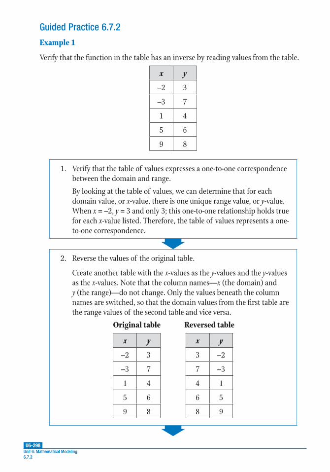
U6-298Unit 6: Mathematical Modeling 6.7.2
Guided Practice 6.7.2
Example 1
Verify that the function in the table has an inverse by reading values from the table.
x y
–2 3
–3 7
1 4
5 6
9 8
1. Verify that the table of values expresses a one-to-one correspondence between the domain and range.
By looking at the table of values, we can determine that for each domain value, or x-value, there is one unique range value, or y-value. When x = –2, y = 3 and only 3; this one-to-one relationship holds true for each x-value listed. Therefore, the table of values represents a one-to-one correspondence.
2. Reverse the values of the original table.
Create another table with the x-values as the y-values and the y-values as the x-values. Note that the column names—x (the domain) and y (the range)—do not change. Only the values beneath the column names are switched, so that the domain values from the first table are the range values of the second table and vice versa.
Original table
x y
–2 3
–3 7
1 4
5 6
9 8
Reversed table
x y
3 –2
7 –3
4 1
6 5
8 9

U6-299Lesson 7: Inverses of Functions
6.7.2
3. Verify whether the values from the reversed table represent a one-to-one correspondence between the variables.
By looking at the new table of values, we can determine that for each domain value, or x-value, there is a unique range value, or y-value. So, when x = 3, y = –2 and only –2; once again, this one-to-one relationship holds true for each x-value listed. Therefore, the table of reversed values shows one-to-one correspondence.
4. Show that the function represented by the reversed table of values is the inverse of the function represented by the original table of values.
Let f(x) represent the first function given in the original table of values.
Recall that f –1(x) is one way to write a possible inverse function.
Let f –1(x) represent the possible inverse function given by the reversed table of values.
In order to show that f –1(x) is the inverse of f(x), by definition of an inverse, we need to show that for (x, y) in the original table, f(f –1(x)) = f –1(f(x)), where f(f –1(x)) will equal the x-value of the given point, and f –1(f(x)) will equal the y-value of the given point. In other words, the input for f(x) is equal to the output of f –1(x) and vice versa.
Let’s start by using the first point from the f(x) table, (–2, 3). Substitute the x- and y-values of this point into f(f –1(x)). Then, substitute the point (3, –2) from the reversed table into f –1(f(x)).
• f(f –1(x)) = f(f –1(3)) = –2, which is equal to the x-value of the given point.
• f –1(f(x)) = f –1(f(–2)) = 3, which is equal to the y-value of the given point.
This relationship can be shown for each of the coordinates in the tables; therefore, f –1(x) is the inverse of f(x).
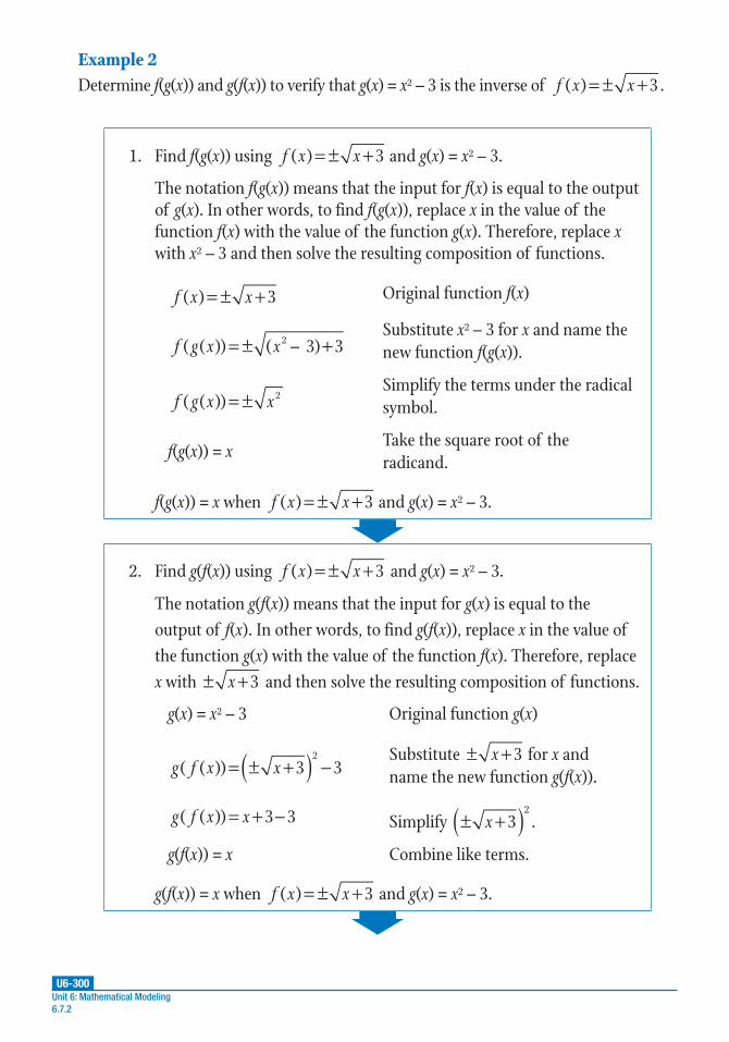
U6-300Unit 6: Mathematical Modeling 6.7.2
Example 2Determine f(g(x)) and g(f(x)) to verify that g(x) = x2 – 3 is the inverse of ( ) 3= ± +f x x .
1. Find f(g(x)) using ( ) 3= ± +f x x and g(x) = x2 – 3.
The notation f(g(x)) means that the input for f(x) is equal to the output of g(x). In other words, to find f(g(x)), replace x in the value of the function f(x) with the value of the function g(x). Therefore, replace x with x2 – 3 and then solve the resulting composition of functions.
( ) 3= ± +f x x Original function f(x)
( ( )) ( – 3) 32= ± +f g x xSubstitute x2 – 3 for x and name the new function f(g(x)).
( ( )) 2= ±f g x xSimplify the terms under the radical symbol.
f(g(x)) = xTake the square root of the radicand.
f(g(x)) = x when ( ) 3= ± +f x x and g(x) = x2 – 3.
2. Find g(f(x)) using ( ) 3= ± +f x x and g(x) = x2 – 3.
The notation g(f(x)) means that the input for g(x) is equal to the output of f(x). In other words, to find g(f(x)), replace x in the value of the function g(x) with the value of the function f(x). Therefore, replace x with 3± +x and then solve the resulting composition of functions.
g(x) = x2 – 3 Original function g(x)
( ( )) 3 32( )= ± + −g f x x
Substitute 3± +x for x and name the new function g(f(x)).
= + −g f x x( ( )) 3 3 Simplify 32( )± +x .
g(f(x)) = x Combine like terms.
g(f(x)) = x when ( ) 3= ± +f x x and g(x) = x2 – 3.

U6-301Lesson 7: Inverses of Functions
6.7.2
3. State a conclusion about whether g(x) is the inverse of f(x) based on the results for f(g(x)) and g(f(x)).
We have determined that f(g(x)) = x and g(f(x)) = x. By substitution, f(g(x)) = g(f(x)); therefore, g(x) is the inverse of f(x).
Example 3
Determine f(g(x)) and g(f(x)) to verify that f(x) = 2x3 – 1 and =+
g xx
( )1
23 are inverses
of each other.
1. Find f(g(x)) using f(x) = 2x3 – 1 and =+
g xx
( )1
23 .
The notation f(g(x)) means that the input for f(x) is equal to the output
of g(x). In other words, to find f(g(x)), replace x in the value of the
function f(x) with the value of the function g(x). Therefore, replace x
with +x 1
23 and then solve the resulting composition of functions.
f(x) = 2x3 – 1 Original function f(x)
=+
−f g x
x( ( )) 2
1
213
3
Substitute +x 1
23 for x and
name the new function f(g(x)).
=+
−f g x
x( ( )) 2
1
21 Apply the exponent to the cube
root.
f(g(x)) = x + 1 – 1 Multiply by 2.
f(g(x)) = x Simplify.
f(g(x)) = x when f(x) = 2x3 – 1 and =+
g xx
( )1
23 .

U6-302Unit 6: Mathematical Modeling 6.7.2
2. Find g(f(x)) using f(x) = 2x3 – 1 and g(x) = +x 1
23 .
The notation g(f(x)) means that the input for g(x) is equal to the output of f(x). In other words, to find g(f(x)), replace x in the value of the function g(x) with the value of the function f(x). Therefore, replace x with 2x3 – 1 and then solve the resulting composition of functions.
=+
g xx
( )1
23 Original function g(x)
=− +
g f xx
( ( ))(2 1) 1
2
3
3Substitute 2x3 – 1 for x and name the new function g(f(x)).
=g f xx
( ( ))2
2
3
3Simplify the numerator of the radicand.
=g f x x( ( )) 33 Simplify the radicand.
g(f(x)) = x Simplify the cube root.
g(f(x)) = x when f(x) = 2x3 – 1 and =+
g xx
( )1
23 .
3. State a conclusion about whether g(x) is the inverse of f(x) based on the results for f(g(x)) and g(f(x)).
We have determined that f(g(x)) = x and g(f(x)) = x. By substitution, f(g(x)) = g(f(x)); therefore, g(x) is the inverse of f(x).

U6-303Lesson 7: Inverses of Functions
6.7.2
Example 4
Determine whether =−
f xx
( )5
2 and =
−g x
x( )
3
5 are inverses.
1. Find f(g(x)) using =−
f xx
( )5
2 and =
−g x
x( )
3
5.
To find f(g(x)), replace x in the value of the function f(x) with the value
of the function g(x). Therefore, replace x with −x 3
5 and then solve the
resulting composition of functions.
=−
f xx
( )5
2Original function f(x)
= −
−
f g xx
( ( ))53
52
Substitute −x 3
5 for x and name
the new function f(g(x)).
( ( ))53
52
•5
5= −
−
f g xx
Simplify the denominator by finding the lowest common denominator of the fraction.
=− −
f g xx
( ( ))25
3 10Multiply the numerator and denominator by the LCD.
==−
f g xx
( ( ))25
13Combine like terms to simplify the denominator.
=−
f g xx
( ( ))25
13 when =
−f x
x( )
5
2 and =
−g x
x( )
3
5.

U6-304Unit 6: Mathematical Modeling 6.7.2
2. Find g(f(x)) using =−
f xx
( )5
2 and =
−g x
x( )
3
5.
To find g(f(x)), replace x in the value of the function g(x) with the value
of the function f(x). Therefore, replace x with −x
5
2 and then solve the
resulting composition of functions.
=−
g xx
( )3
5Original function g(x)
=−
−
g f xx
( ( ))
5
23
5
Substitute −x
5
2 for x and name
the new function g(f(x)).
=−
− −
−g f x
x x
x( ( ))
5
23
5•
5( 2)
5( 2)
Simplify the numerator by finding the lowest common denominator of the fraction.
=− −
−g f x
x
x( ( ))
25 15( 2)
25( 2)Multiply the numerator and denominator by the LCD.
=− +
−g f x
x
x( ( ))
25 15 30
25 50Multiply to simplify the numerator and denominator.
=−−
g f xx
x( ( ))
55 15
25 50Combine like terms.
=−−
g f xx
x( ( ))
11 3
5 10Factor 5 from each term in the numerator and denominator.
=−−
g f xx
x( ( ))
11 3
5 10 when =
−f x
x( )
5
2 and =
−g x
x( )
3
5.
3. State a conclusion about whether g(x) is the inverse of f(x) based on the results for f(g(x)) and g(f(x)).
We have determined that =−
f g xx
( ( ))25
13 and
=−−
g f xx
x( ( ))
11 3
5 10; since f(g(x)) ≠ g(f(x)), neither function is
the inverse of the other.

U6-305Lesson 7: Inverses of Functions
6.7.2
Example 5
Given f(x) = x2 – 4 and = +g x x( ) 4 , show by graphing that g(x) is the inverse of f(x) only when the domain is restricted. Use the graph of the two functions to state the restricted domain.
1. Graph f(x) = x2 – 4 and = +g x x( ) 4 together on a coordinate plane.
Graph the functions either by hand or with a graphing calculator. The resulting graph should resemble the following.
8
6
4
2
–2
–4
–6
–8
8642–2–4–6–8 0
y
x
f(x)
g(x)

U6-306Unit 6: Mathematical Modeling 6.7.2
2. Show that g(x) is only an inverse of f(x) when the domain is restricted using a line of symmetry. Use the graph of the two functions to state the restricted domain.
Add the line y = x to the graph to see where the two graphed functions are symmetrical.
8
6
4
2
–2
–4
–6
–8
8642–2–4–6–8 0
y
x
f(x)
g(x)
y = x
Notice that the functions are symmetrical about the line y = x only on the right side of the x-axis; that is, when x ≥ 0 (as shown in bold). Notice that f(x) is only one-to-one for x ≥ 0 or for x ≤ 0. Therefore, g(x) is only an inverse of f(x) when the domain is restricted to x-values greater than or equal to 0.
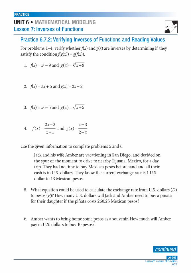
U6-307
PRACTICE
UNIT 6 • MATHEMATICAL MODELINGLesson 7: Inverses of Functions
Lesson 7: Inverses of Functions6.7.2
For problems 1–4, verify whether f(x) and g(x) are inverses by determining if they satisfy the condition f(g(x)) = g(f(x)).
1. f(x) = x3 – 9 and = +g x x( ) 93
2. f(x) = 3x + 5 and g(x) = 2x – 2
3. f(x) = x2 – 5 and = +g x x( ) 5
4. =−+
f xx
x( )
2 3
1 and =
+−
g xx
x( )
3
2
Use the given information to complete problems 5 and 6.
Jack and his wife Amber are vacationing in San Diego, and decided on the spur of the moment to drive to nearby Tijuana, Mexico, for a day trip. They had no time to buy Mexican pesos beforehand and all their cash is in U.S. dollars. They know the current exchange rate is 1 U.S. dollar to 13 Mexican pesos.
5. What equation could be used to calculate the exchange rate from U.S. dollars (D) to pesos (P)? How many U.S. dollars will Jack and Amber need to buy a piñata for their daughter if the piñata costs 260.25 Mexican pesos?
6. Amber wants to bring home some pesos as a souvenir. How much will Amber pay in U.S. dollars to buy 10 pesos?
continued
Practice 6.7.2: Verifying Inverses of Functions and Reading Values
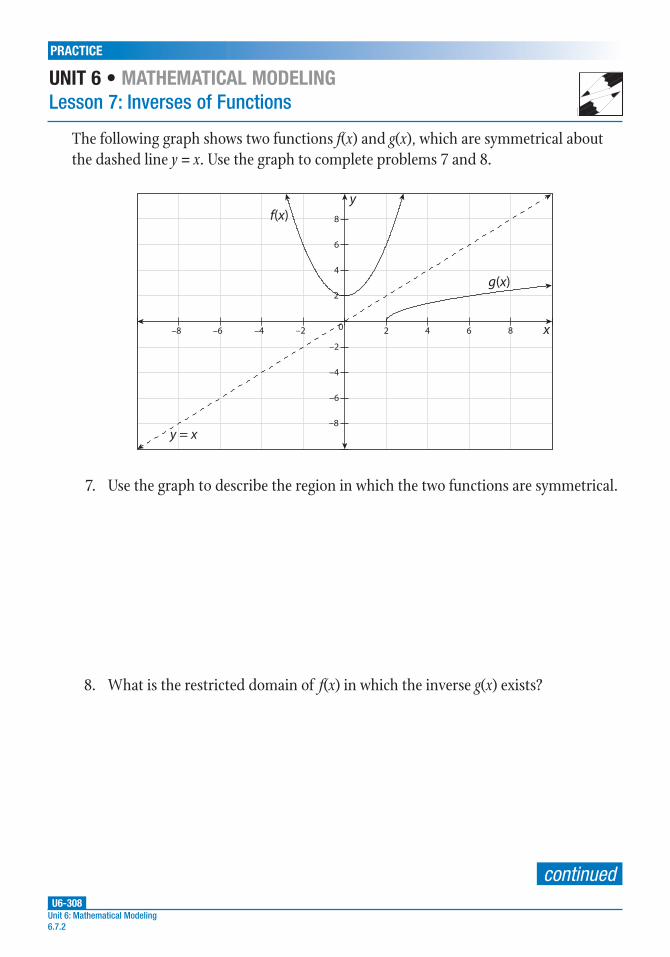
U6-308
PRACTICE
UNIT 6 • MATHEMATICAL MODELINGLesson 7: Inverses of Functions
Unit 6: Mathematical Modeling 6.7.2
The following graph shows two functions f(x) and g(x), which are symmetrical about the dashed line y = x. Use the graph to complete problems 7 and 8.
y
x0
g(x)
f(x)
y = x
8
6
4
2
–2
–4
–6
–8
–2–4–6–8 8642
7. Use the graph to describe the region in which the two functions are symmetrical.
8. What is the restricted domain of f(x) in which the inverse g(x) exists?
continued
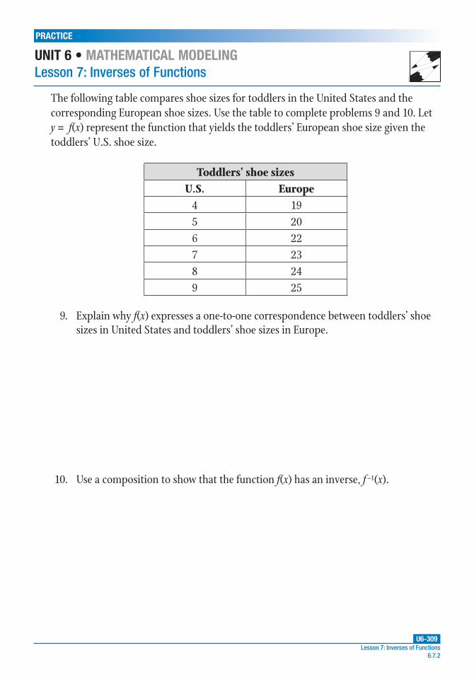
U6-309
PRACTICE
UNIT 6 • MATHEMATICAL MODELINGLesson 7: Inverses of Functions
Lesson 7: Inverses of Functions6.7.2
The following table compares shoe sizes for toddlers in the United States and the corresponding European shoe sizes. Use the table to complete problems 9 and 10. Let y = f(x) represent the function that yields the toddlers’ European shoe size given the toddlers’ U.S. shoe size.
Toddlers’ shoe sizesU.S. Europe
4 195 206 227 238 249 25
9. Explain why f(x) expresses a one-to-one correspondence between toddlers’ shoe sizes in United States and toddlers’ shoe sizes in Europe.
10. Use a composition to show that the function f(x) has an inverse, f –1(x).

Lesson 8: Geometric ModelingUNIT 6 • MATHEMATICAL MODELING
U6-310Unit 6: Mathematical Modeling6.8
Common Core Georgia Performance Standards
MCC9–12.G.GMD.4
MCC9–12.G.MG.1★
MCC9–12.G.MG.2★
MCC9–12.G.MG.3★
Essential Questions
1. What plane geometric figure is formed when a plane intersects a solid figure?
2. What solid figure is formed when a plane figure is rotated a specific number of degrees or radians?
3. How can the density of a quantity be computed for the area or volume in which the quantity is located?
4. How can density be used to compute the total amount of a quantity in an area or a volume?
5. How can the properties of geometric figures and their measurements be used to design solutions to real-world problems?
WORDS TO KNOW
axis of rotation a line about which a plane figure can be rotated in three-dimensional space to create a solid figure, such as a diameter or a symmetry line
congruent having the same shape, size, lines, and angles; the symbol for representing congruency between figures is ≅
cross section the plane figure formed by the intersection of a plane with a solid figure, where the plane is at a right angle to the surface of the solid figure
density the amount, number, or other quantity per unit of area or volume of some substance or population being studied

U6-311Lesson 8: Geometric Modeling
6.8
plane a flat, two-dimensional figure without depth that has at least three non-collinear points and extends infinitely in all directions
plane figure a two-dimensional shape on a plane
polyhedron a three-dimensional object that has faces made of polygons
regular polyhedron a polyhedron with faces that are all congruent regular polygons; the angles created by the intersecting faces are congruent, and the cross sections are similar figures
rho (ρ) a lowercase Greek letter commonly used to represent density
rotation in three dimensions, a transformation in which a plane figure is moved about one of its sides, a fixed point, or a line that is not located in the plane of the figure, such that a solid figure is produced
similar figures two figures that are the same shape but not necessarily the same size; the symbol for representing similarity between figures is .
solid figure a three-dimensional object that has length, width, and height (depth)
translation in three dimensions, the horizontal or vertical movement of a plane figure in a direction that is not in the plane of the figure, such that a solid figure is produced

U6-312Unit 6: Mathematical Modeling6.8
Recommended Resources
• Annenberg Learner. “Cross Sections.”
http://www.walch.com/rr/00249
This site provides an overview of cross sections, along with an interactive cube that can be rotated and cut in various locations to show the resulting cross section. Requires Flash.
• LearnZillion.com. “Predict 3D Results of Rotating Simple Figures.”
http://www.walch.com/rr/00250
This video tutorial reviews how rotations of a plane figure about an axis can be used to create three-dimensional solids.
• MathIsFun.com. “Solid Geometry.”
http://www.walch.com/rr/00251
This site reviews the geometry of three-dimensional objects; in particular, it covers properties of solids and compares polyhedra to non-polyhedra, with examples of each.

U6-313Lesson 8: Geometric Modeling
6.8.1
Lesson 6.8.1: Two-Dimensional Cross Sections of Three-Dimensional ObjectsIntroduction
A chef takes a knife and slices a carrot in half. What shape results? Depending on the direction of the cut, the resulting shape may resemble a circle (for a widthwise cut), a triangle (for a lengthwise cut from the tip of the carrot to its base), or an oval (for a diagonal cut). The circle, triangle, and oval are each a type of plane figure, a two-dimensional shape on a plane. Recall that a plane is a flat, two-dimensional figure without depth that has at least three non-collinear points and extends infinitely in all directions. When planes intersect with solid figures, or three-dimensional objects that have length, width, and height (or depth), plane figures are created. In this example, the carrot can be thought of as the solid figure, the knife as the intersecting plane, and the resulting shape as the plane figure.
Plane figures have many applications in real-world problems. Technical drawings of solid figures, such as the parts of a redesigned spacecraft, often rely on back, bottom, front, and rear views of a figure that exists in three dimensions or in three-dimensional coordinate systems. These applications can be as complex as the real-world circumstances in which they are found, but many rely on relatively basic properties of plane and solid geometry for their description and use in calculations.
Similarly, two-dimensional figures can be used to generate solid figures with transformations in three-dimensional space. Solids can be generated by the horizontal or vertical movement of a plane figure through a third dimension, or by the rotation of a plane figure about an axis of rotation or line in a third dimension.
Key Concepts
• In its basic form, a cross section is the plane figure formed by the intersection of a plane and a solid figure, where the plane is at a right angle to the surface of the solid figure. The cross section can also be formed by an axis of rotation of the solid figure, given that the axis of rotation is perpendicular to the intersecting plane.
• An axis of rotation is a line about which a plane figure can be rotated in three-dimensional space to create a solid figure, such as a diameter or a symmetry line. For example, a line that connects the centers of the circular bases of a cylinder is an axis of rotation.
• The shape of a cross section depends on the solid figure and the location of the cross section.
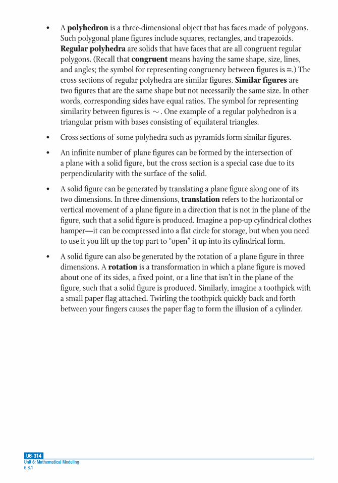
U6-314Unit 6: Mathematical Modeling6.8.1
• A polyhedron is a three-dimensional object that has faces made of polygons. Such polygonal plane figures include squares, rectangles, and trapezoids. Regular polyhedra are solids that have faces that are all congruent regular polygons. (Recall that congruent means having the same shape, size, lines, and angles; the symbol for representing congruency between figures is ≅.) The cross sections of regular polyhedra are similar figures. Similar figures are two figures that are the same shape but not necessarily the same size. In other words, corresponding sides have equal ratios. The symbol for representing similarity between figures is . One example of a regular polyhedron is a triangular prism with bases consisting of equilateral triangles.
• Cross sections of some polyhedra such as pyramids form similar figures.
• An infinite number of plane figures can be formed by the intersection of a plane with a solid figure, but the cross section is a special case due to its perpendicularity with the surface of the solid.
• A solid figure can be generated by translating a plane figure along one of its two dimensions. In three dimensions, translation refers to the horizontal or vertical movement of a plane figure in a direction that is not in the plane of the figure, such that a solid figure is produced. Imagine a pop-up cylindrical clothes hamper—it can be compressed into a flat circle for storage, but when you need to use it you lift up the top part to “open” it up into its cylindrical form.
• A solid figure can also be generated by the rotation of a plane figure in three dimensions. A rotation is a transformation in which a plane figure is moved about one of its sides, a fixed point, or a line that isn’t in the plane of the figure, such that a solid figure is produced. Similarly, imagine a toothpick with a small paper flag attached. Twirling the toothpick quickly back and forth between your fingers causes the paper flag to form the illusion of a cylinder.

U6-315Lesson 8: Geometric Modeling
6.8.1
Guided Practice 6.8.1Example 1
Compare the areas of two rectangular cross sections of an air-conditioning duct along a length of the duct that shrinks in width from 20 inches to 12 inches and in height from 8 inches to 6 inches. Find the difference of the areas, and determine the percentage that each cross section is of the other. Then, name the solid figure from which the two rectangular cross sections are formed.
20 in
12 in
6 in
8 in
1. Calculate the area of the larger cross section.
The larger cross section is a rectangle, so use the formula for the area of a rectangle, area = length • width. In this case, the “length” is actually the height, so use the formula area = height • width, or A = hw.
The larger cross section has a height of 8 inches and a width of 20 inches. Substitute these measurements into the formula A = hw and then solve to determine the area of the larger cross section.
A = hw Rectangular area formula
A = (8)(20) Substitute 8 for h and 20 for w.
A = 160 Simplify.
Recall that area is expressed in square units.
Thus, the area of the larger cross section is 160 square inches.

U6-316Unit 6: Mathematical Modeling6.8.1
2. Calculate the area of the smaller cross section.
The smaller cross section is also a rectangle, so use the formula A = hw. However, this cross section has a height of 6 inches and a width of 12 inches. Substitute these measurements into the formula A = hw and then solve to determine the area of the smaller cross section.
A = hw Rectangular area formula
A = (6)(12) Substitute 6 for h and 12 for w.
A = 72 Simplify.
The area of the smaller cross section is 72 square inches.
3. Find the difference of the cross section areas.
Subtract the area of the smaller cross section from the area of the larger cross section.
160 – 72 = 88
The difference of the areas is 88 square inches.
4. Calculate the percentage that the smaller area is of the larger area.
Divide the smaller area by the larger area and then multiply by 100 to find the percentage.
smaller area
larger area•100 Percentage formula
72
160•100
( )( )
= Substitute 72 for the smaller area and 160 for the larger area.
= 45 Simplify.
The smaller area is 45% of the size of the larger area.

U6-317Lesson 8: Geometric Modeling
6.8.1
Example 2
The diagram shows the two cross sections, I and II, of a solid figure. What is the geometric solid from which the cross sections are formed?
2 m6 m 4 mII
I
6 m
5. Calculate the percentage that the larger area is of the smaller area.
Divide the larger area by the smaller area and then multiply by 100 to find the percentage.
larger area
smaller area•100 Percentage formula
160
72•100
( )( )
= Substitute 160 for the larger area and 72 for the smaller area.
≈ 222.2 Simplify.
The larger area is about 222% of the size of the smaller area.
6. Determine the solid figure from which the cross sections are formed.
The areas of the rectangular cross sections are unequal, and the rectangular cross sections are not similar. Given this information, the only solid figure from which these cross sections could have been formed is like a pyramid with a rectangular base, except that instead of coming to a point at the top, it comes to a line like the ridge of a roof.
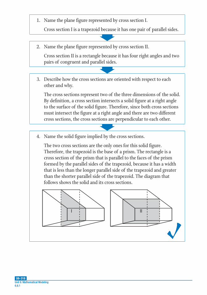
U6-318Unit 6: Mathematical Modeling6.8.1
1. Name the plane figure represented by cross section I.
Cross section I is a trapezoid because it has one pair of parallel sides.
2. Name the plane figure represented by cross section II.
Cross section II is a rectangle because it has four right angles and two pairs of congruent and parallel sides.
3. Describe how the cross sections are oriented with respect to each other and why.
The cross sections represent two of the three dimensions of the solid. By definition, a cross section intersects a solid figure at a right angle to the surface of the solid figure. Therefore, since both cross sections must intersect the figure at a right angle and there are two different cross sections, the cross sections are perpendicular to each other.
4. Name the solid figure implied by the cross sections.
The two cross sections are the only ones for this solid figure. Therefore, the trapezoid is the base of a prism. The rectangle is a cross section of the prism that is parallel to the faces of the prism formed by the parallel sides of the trapezoid, because it has a width that is less than the longer parallel side of the trapezoid and greater than the shorter parallel side of the trapezoid. The diagram that follows shows the solid and its cross sections.
III
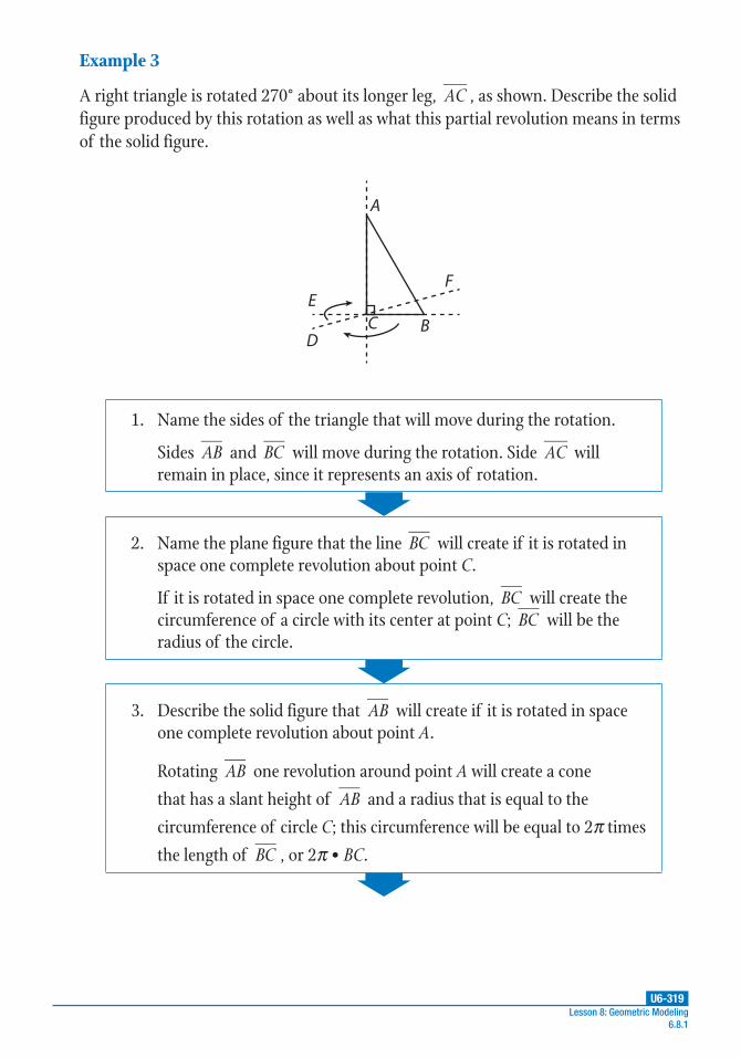
U6-319Lesson 8: Geometric Modeling
6.8.1
Example 3
A right triangle is rotated 270° about its longer leg, AC , as shown. Describe the solid figure produced by this rotation as well as what this partial revolution means in terms of the solid figure.
A
F
BCD
E
1. Name the sides of the triangle that will move during the rotation.
Sides AB and BC will move during the rotation. Side AC will remain in place, since it represents an axis of rotation.
2. Name the plane figure that the line BC will create if it is rotated in space one complete revolution about point C.
If it is rotated in space one complete revolution, BC will create the circumference of a circle with its center at point C; BC will be the radius of the circle.
3. Describe the solid figure that AB will create if it is rotated in space one complete revolution about point A.
Rotating AB one revolution around point A will create a cone
that has a slant height of AB and a radius that is equal to the
circumference of circle C; this circumference will be equal to 2π times
the length of BC , or 2π • BC.
U6-320Unit 6: Mathematical Modeling6.8.1
4. Describe the solid figure produced by the rotation.
The solid figure is a cone with a highest point at point A, a height of AC , and a circular base with a radius of length BC .
5. Determine what fraction of a complete revolution 270° represents.
Recall that 270° is the number of degrees that the lines AB and BC
rotate. Multiply 270° by the conversion factor 1 revolution
360° to convert
the degree measure to revolutions.
2701 revolution
360
3
4revolution°•
°=
270° is equivalent to 3
4 of a complete revolution.
6. Describe what this partial revolution means in terms of the solid figure.
A 270° revolution of the right triangle results in a figure that is 3
4 of
the cone that would be produced if the right triangle were
rotated by one complete revolution.
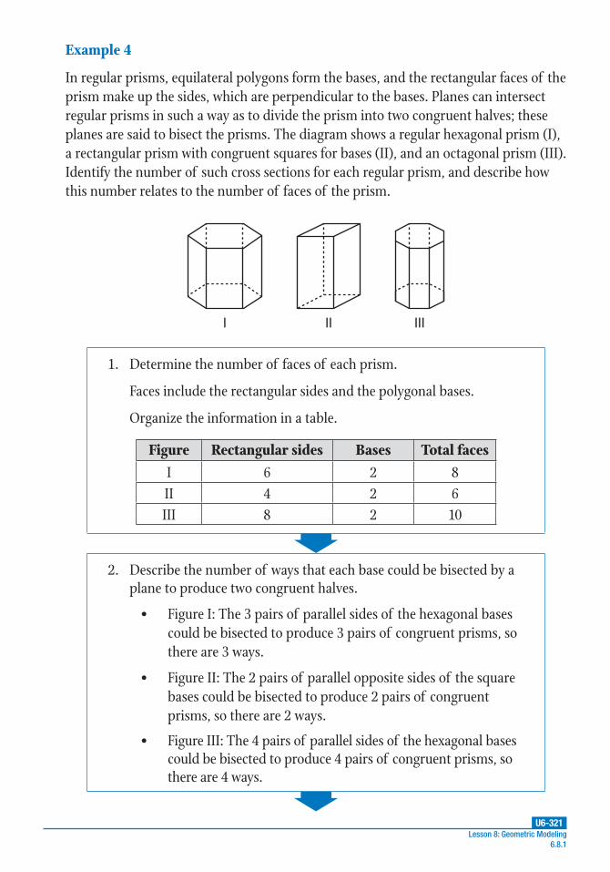
U6-321Lesson 8: Geometric Modeling
6.8.1
Example 4
In regular prisms, equilateral polygons form the bases, and the rectangular faces of the prism make up the sides, which are perpendicular to the bases. Planes can intersect regular prisms in such a way as to divide the prism into two congruent halves; these planes are said to bisect the prisms. The diagram shows a regular hexagonal prism (I), a rectangular prism with congruent squares for bases (II), and an octagonal prism (III). Identify the number of such cross sections for each regular prism, and describe how this number relates to the number of faces of the prism.
I II III
1. Determine the number of faces of each prism.
Faces include the rectangular sides and the polygonal bases.
Organize the information in a table.
Figure Rectangular sides Bases Total facesI 6 2 8II 4 2 6III 8 2 10
2. Describe the number of ways that each base could be bisected by a plane to produce two congruent halves.
• Figure I: The 3 pairs of parallel sides of the hexagonal bases could be bisected to produce 3 pairs of congruent prisms, so there are 3 ways.
• Figure II: The 2 pairs of parallel opposite sides of the square bases could be bisected to produce 2 pairs of congruent prisms, so there are 2 ways.
• Figure III: The 4 pairs of parallel sides of the hexagonal bases could be bisected to produce 4 pairs of congruent prisms, so there are 4 ways.

U6-322Unit 6: Mathematical Modeling6.8.1
3. Describe the number of ways that each prism could be bisected by a plane that is parallel to the bases to produce two congruent halves.
To produce two congruent prisms, each figure could be intersected by 1 plane located halfway between and parallel to the bases. Therefore, there is only 1 way this is possible for each prism.
4. Use the results of steps 2 and 3 to determine the total number of cross sections that produce congruent halves of each prism.
Add the number of ways each prism’s base could be bisected (found in step 2) to the number of ways each prism could be bisected (step 3). This gives the total number of cross sections that produce congruent halves.
• Figure I: 3 + 1 = 4 cross sections
• Figure II: 2 + 1 = 3 cross sections
• Figure III: 4 + 1 = 5 cross sections
5. Use the results number of faces and cross sections for each figure to suggest a rule relating the total number of faces to the number of cross sections that produce congruent prisms.
Refer to the table from step 1 and the results of step 4 to determine the number of faces and cross sections.
• Figure I has 8 faces and 4 cross sections.
• Figure II has 6 faces and 3 cross sections.
• Figure III has 10 faces and 5 cross sections
Based on these figures, the rule appears to be that the number of cross sections producing congruent prisms is half of the number of faces of the “parent” prism.
6. Use the number of faces and cross sections result for Figure II to predict how many cross sections would be needed to divide a regular decagonal (10-sided) prism into congruent halves.
Based on these results, the number of cross sections would be half the number of faces of the decagonal prism. A decagonal prism has 10 rectangular faces and 2 bases, for a total of 12 faces. Therefore, 6 cross sections would be needed to divide the regular decagonal prism into congruent halves.

U6-323
PRACTICE
UNIT 6 • MATHEMATICAL MODELINGLesson 8: Geometric Modeling
Lesson 8: Geometric Modeling6.8.1
For problems 1–4, calculate the area of the cross section for each object described.
1. a cross section that is located halfway between the bases of a prism that are congruent triangles with two sides that are 5 inches in length and a third side that is 6 inches in length
2. the two cross sections of unequal areas of a rectangular solid with dimensions of 2 meters by 2 meters by 7 meters
3. a cross section that is located a distance of 1
π yard from the center of a sphere
with a volume of 36π cubic yards
4. the cross section of a regular hexagonal prism that is inscribed in a cylinder of radius 20 centimeters
For problems 5–7, use the diagram to describe the object formed by rotating each given figure one complete revolution about line l.
lC
BA
G F
E
D
5. arc FG
6. sector FDE
7. triangle ABC
Practice 6.8.1: Two-Dimensional Cross Sections of Three-Dimensional Objects
continued

U6-324
PRACTICE
UNIT 6 • MATHEMATICAL MODELINGLesson 8: Geometric Modeling
Unit 6: Mathematical Modeling6.8.1
For problems 8–10, calculate the quantity indicated.
8. the cross sections of least and greatest area for a rectangular block of marble with dimensions of 1 meter by 2 meters by 3 meters
9. the maximum diameter of a cross section of a spherical polyester bead that has a volume of 25π cubic microns
10. the dimensions of a rectangular anode “target” in a photoelectric cell that has a cross section of 10–18 m2 if the dimensions of the anode have a 3-to-1 ratio

U6-325Lesson 8: Geometric Modeling
6.8.2
Introduction
Density is used in a variety of fields to quantify the amount, number, or other quantity per unit of area, volume, or some other basic variable. In some situations, density is used to compare the total number of a quantity with the average value of the quantity when it is associated with a second variable. In real-world problems, it is important to carefully define the quantity being averaged, especially with regard to what kind(s) of numbers can be used for quantification. In this sub-lesson, the density of a quantity will be most often compared to a basic unit of area or volume, but these are by no means the only way of averaging a quantity.
Key Concepts
• Density is the amount, number, or other quantity per unit of area or volume of some substance or population being studied.
• Density is often symbolized with the lowercase Greek letter rho (ρ).
• In many real-world problems, density is used to calculate an average value of
some quantity in terms of a basic unit of area or volume.
• The most basic units of density for these two types of calculations are given by the following formulas:
Equation in words Equation in symbols
Densitymass or quantity
number of unitsArea =square
ρ =m
AA
Densitymass or quantity
number of unitsVolume =cubic
m
VVρ =
• Note that these formulas are quite similar, but the area density formula divides by the area, A, (square units) and the volume density formula divides by the volume, V (cubic units). Keeping this distinction in mind can be a useful guide in writing equations for many different density situations.
• Density can vary considerably from one place to another in an area or volume of interest, so it is important to determine if the density calculation will be meaningful for a situation as a whole or if the calculation cannot be reliably used to describe variations in a quantity per unit throughout a problem setting.
Lesson 6.8.2: Density

U6-326Unit 6: Mathematical Modeling6.8.2
• Sometimes the domain of a quantity can determine the most appropriate basic unit to use in order for a density calculation to be meaningful. Fractions of a counting number may be unrealistic for a given situation, such as determining the population density of people living in a certain square mile of a city. Density calculations in such situations make more sense if the contexts in which the quantity is averaged or in which the density is calculated are changed to accommodate the smallest meaningful unit of a quantity of interest.

U6-327Lesson 8: Geometric Modeling
6.8.2
Guided Practice 6.8.2Example 1
A laser-jet printer uses 7,500 droplets of soy-based printer ink to deposit a 6-inch long line of type that is an average of 0.125 of an inch high. How many droplets of ink are deposited per square inch?
1. Calculate the area represented by the line of type.
The area is the product of the height, 6 inches, and the length of the line of type, 0.125 inch.
6 inches • 0.125 inch = 0.75 square inches
2. Use the area to calculate the density of ink drops per square inch.
Recall that density is equal to some quantity divided by the area unit.
Here, we’re dealing with the two-dimensional area of a piece of paper,
so use the formula Densityquantity
number of square unitsArea = .
The number of drops, or quantity, is given as 7,500.
The area, or number of square units, is 0.75.
Substitute these values into the formula to calculate the density.
Densityquantity
number of square unitsArea = Area density formula
Density7500
0.75Area =Substitute 7,500 for the quantity and 0.75 for the number of square units.
Density 10,000Area = Simplify.
The ink-jet printer has a print density of 10,000 droplets per square inch.

U6-328Unit 6: Mathematical Modeling6.8.2
Example 2
There are 35,000 bats roosting in a pyramid-shaped vaulted cave ceiling that has a height of 30 meters and a rectangular floor that measures 75 by 100 meters. What is the average density of the bat population in the cave? Make sure that the density is a number that reflects the fact that the bat population is measured in counting numbers.
1. Calculate the volume of the cave.
The cave is pyramid-shaped, with a rectangular floor representing the base of the pyramid.
Recall that the volume of a pyramid is found using the formula 1
3=V Ah , where A is the area of the base of the pyramid and h is the
pyramid’s height.
The rectangular floor’s area can be found using the formula A = lw, so use lw for the area, A, substitute the known values, and solve for the volume.
1
3=V Ah Pyramid volume formula
1
3( )=V lw h Substitute lw for A.
1
3(75)(100)(30)=V Substitute 75 for l, 100 for w, and 30 for h.
V = 75,000 Simplify.
The pyramid-shaped cave has a volume of 75,000 cubic meters.
U6-329Lesson 8: Geometric Modeling
6.8.2
2. Calculate the volume density of the bats in the cave.
Use the formula Densityquantity
number of cubic unitsVolume = .
The number of bats, or the quantity, is given as 35,000.
The volume of the cave is 75,000 cubic meters.
Substitute these values into the formula to calculate the density.
Densityquantity
number of cubic unitsVolume = Volume density formula
Density35,000
75,000Volume
( )( )=
Substitute 35,000 for the quantity and 75,000 for the number of cubic units.
Density 0.46Volume = Simplify.
The average density of the bat population in the cave is 0.46 bats per cubic meter.
3. Determine the domain of the bat population.
The bat population consists of individual bats that are counted using positive integers. Therefore, the domain of the bat population is [1, 35,000].
4. Suggest a different basic volume unit that will result in a bat density measured in positive integers.
One option for the basic volume unit could be a 2 × 2 × 2 meter space
within the cave (8 m3) rather than 1 cubic meter. We can write this
conversion factor as a ratio, 1 unit of volume
8 cubic meters.
U6-330Unit 6: Mathematical Modeling6.8.2
5. Use the response to step 4 to calculate a more realistic value for the bat density.
Start by converting the total volume of the cave to the new unit of volume measurement.
75,000 cubic meters •1 volume unit
8 cubic meters
Multiply the volume of the cave by the conversion ratio from step 4.
9,375 volume units Simplify.
Next, substitute the new volume units into the volume formula for the density and recalculate the density. Since the number of bats in the total volume of the cave is unchanged, use 35,000 for the bat quantity.
Densityquantity
number of cubic unitsVolume = Volume density formula
Density35,000
9,375Volume
( )( )=
Substitute 35,000 for the quantity of bats and 9,375 for the volume units.
Density 3.73Volume = Simplify.
Therefore, there are approximately 3.73 bats per 1 volume unit, which was defined as 8 m3.
Rounded up to the nearest whole integer, the new calculation gives a density of about 4 bats for each 8 cubic meter space of the cave.
6. Compare the number of bats predicted by the result of step 5 to the number of bats given in the problem.
Multiply the total number of volume units in the cave (9,375 volume units) by the estimated number of bats per volume unit from step 5 (4 bats) to determine the total predicted number of bats in the cave.
9375 volume units •4 bats
1 volume unit37,500=
Based on our estimate, there are about 37,500 bats in the cave. The original problem gave a bat population of 35,000. Therefore, the estimated population of 37,500 bats is about 7% greater than the given population of 35,000 bats. This is a realistic measurement.

U6-331Lesson 8: Geometric Modeling
6.8.2
Example 3
Manatees are known to gather in the warmer waters surrounding power plants, which dispose of heated wastewater using discharge canals. The diagram shows the distribution of manatees on a cool winter day in the hot-water discharge basin surrounding a Gulf Coast power plant, as seen on an aerial security photograph. The plant’s discharge canal is marked by an X at the end of the positive y-axis. Each data point represents 10 manatees, and each quadrant represents an area measuring 50 yards by 50 yards.
–50 –40 –30 –20 –10 10 20 30 40 50
x
50
40
30
20
10
0
–10
–20
–30
–40
–50
yDischarge canal
III
IV
X
III
Calculate the density of manatees in each of the four quadrants. Then, calculate the average density of the manatees for all four combined quadrants that make up the discharge basin. Contrast and compare the densities, explain any variations, and make note of any other factors that should be included in relation to the reasonableness of the results and units.
1. Calculate the area of each quadrant.
Each quadrant has an area of 50 yards • 50 yards, or 2,500 square yards.
2. Write the area density formula using the variable names for the problem.
The area density formula is Densitynumber of manatees
number of square yardsArea = .
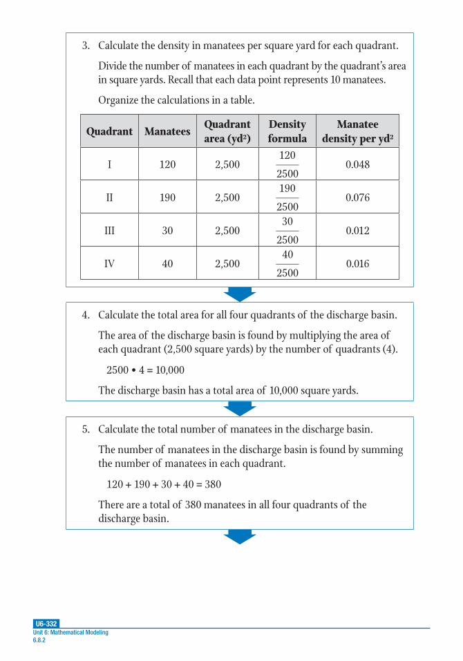
U6-332Unit 6: Mathematical Modeling6.8.2
3. Calculate the density in manatees per square yard for each quadrant.
Divide the number of manatees in each quadrant by the quadrant’s area in square yards. Recall that each data point represents 10 manatees.
Organize the calculations in a table.
Quadrant ManateesQuadrant area (yd2)
Density formula
Manatee density per yd2
I 120 2,500120
25000.048
II 190 2,500190
25000.076
III 30 2,50030
25000.012
IV 40 2,50040
25000.016
4. Calculate the total area for all four quadrants of the discharge basin.
The area of the discharge basin is found by multiplying the area of each quadrant (2,500 square yards) by the number of quadrants (4).
2500 • 4 = 10,000
The discharge basin has a total area of 10,000 square yards.
5. Calculate the total number of manatees in the discharge basin.
The number of manatees in the discharge basin is found by summing the number of manatees in each quadrant.
120 + 190 + 30 + 40 = 380
There are a total of 380 manatees in all four quadrants of the discharge basin.
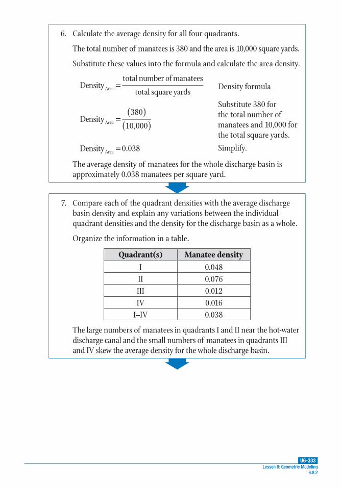
U6-333Lesson 8: Geometric Modeling
6.8.2
6. Calculate the average density for all four quadrants.
The total number of manatees is 380 and the area is 10,000 square yards.
Substitute these values into the formula and calculate the area density.
Densitytotal number of manatees
total square yardsArea = Density formula
Density380
10,000Area
( )( )=
Substitute 380 for the total number of manatees and 10,000 for the total square yards.
Density 0.038Area = Simplify.
The average density of manatees for the whole discharge basin is approximately 0.038 manatees per square yard.
7. Compare each of the quadrant densities with the average discharge basin density and explain any variations between the individual quadrant densities and the density for the discharge basin as a whole.
Organize the information in a table.
Quadrant(s) Manatee density I 0.048II 0.076III 0.012IV 0.016
I–IV 0.038
The large numbers of manatees in quadrants I and II near the hot-water discharge canal and the small numbers of manatees in quadrants III and IV skew the average density for the whole discharge basin.

U6-334Unit 6: Mathematical Modeling6.8.2
8. Explain how to change the density formulas so that the densities can be expressed in “whole” manatees.
The area of the discharge basin could be re-scaled so that the basic area unit is small enough to yield manatee densities that are greater than 1. For example, by defining the basic unit of area as a 10-yard by 10-yard area (100 square yards), the resulting density numbers would be greater than 1. This would give a density of about 5 manatees per 100 square yards in Quadrant I, about 8 manatees in Quadrant II, about 1 manatee in Quadrant III, and about 2 manatees in Quadrant IV. The overall density would be about 4 manatees in each 100-square-yard area.
Example 4
The table shows five different volume densities of water taken from an inland salt lake, in kilograms per cubic meter. The samples were all taken at locations that are equidistant and representative of the overall dimensions of the lake. Determine the average saltwater density for the lake.
Density (kg/m3) Number of samples Weighted samples
(density • samples) (kg/m3)1,020 12 12,2401,022 20 20,4401,025 15 15,3751,030 22 22,6601,032 16 16,512
1. Describe how the number of samples for each density affects the average density.
The numbers of samples “weight” the densities they represent, such that a large number of samples for any one density will have a greater effect on the average density. Thus, the 22 samples with a density of 1,030 kilograms per cubic meter will have a greater effect on the average density than the smaller samples collected for the other four densities. However, a combination of any two other densities will have a “weight” greater than that of 1,030 kilograms per cubic meter.

U6-335Lesson 8: Geometric Modeling
6.8.2
2. Calculate the average saltwater density for the lake.
First, determine the total number of samples by summing them.
12 + 20 + 15 + 22 + 16 = 85
The total number of samples is 85.
Next, find the sum of the weighted samples. All samples are in kg/m3.
12,240 + 20,440 + 15,375 + 22,660 + 16,512 = 87,227
The sum of the weighted samples is 87,227 kg/m3.
Calculate the average by dividing sum of the weighted samples by the total number of samples.
87,227
851026.2= kg/m3
The average saltwater density of the lake is 1,026.2 kilograms per cubic meter, or 1,026 kilograms per cubic meter. Interpret the average saltwater density of the samples in terms of the overall saltwater density of the lake.
Based on these five densities taken in a total of 85 representative samples, the average saltwater density of the lake is about 1,026 kilograms per cubic meter.

U6-336
PRACTICE
UNIT 6 • MATHEMATICAL MODELINGLesson 8: Geometric Modeling
Unit 6: Mathematical Modeling6.8.2
Use the information given in each scenario to complete problems 1–4.
1. The proverbial “tip of the iceberg” visible above water represents a small part of the volume of the total iceberg; most of it is submerged. Calculate the percentage of an iceberg that is above the water line if the density of ice is 925 kilograms per cubic meter and the density of water is 1,000 kilograms per cubic meter.
2. A mechanic exerts 20 pounds of force on a 2-inch square column of hydraulic fluid in a hydraulic lift. The force in the column of fluid is transmitted to a rectangular load platform that measures 3 feet by 4 feet. How much weight can be lifted if all of the force goes into lifting the load on the platform?
3. The electric scanning “eye” of an early moon lander was in the shape of a trapezoid with its two parallel pairs of sides having dimensions of 3 centimeters and 4 centimeters. Its height was 5 centimeters. The amount of light reaching the eye was reduced by moon dust that was stirred up when the lander reached the moon’s surface. Calculate the new effective scanning area of the electric eye if the output of the eye was reduced from 12 volts to 8 volts.
4. A prospector takes a bag of metal nuggets (gold alloyed with mercury) from his claim to the assayer’s office to be valued. What percentage of his metal is gold if it assays out at 18 grams per cubic centimeter? (Note: The density of pure gold is 19,300 kilograms per cubic meter and the density of pure mercury is 13,600 kilograms per cubic meter.)
Practice 6.8.2: Density
continued

U6-337
PRACTICE
UNIT 6 • MATHEMATICAL MODELINGLesson 8: Geometric Modeling
Lesson 8: Geometric Modeling6.8.2
Use the information that follows to complete problems 5–10.
Doughnuts browned in hot vegetable oil are flipped during the cooking process so that each doughnut is evenly cooked throughout. After it is flipped, a white line of uncooked dough forms on the edge of the doughnut. That line can be used to determine the relationship between the density of the doughnut and the density of the oil. Suppose that a cylindrical doughnut stick with a height of 4 cm is laid flat in cooking oil such that the white line appears w centimeters from the bottom of the doughnut stick. The density of the vegetable oil (ρoil) is 925 kilograms per cubic meter and the doughnut stick’s density (ρdoughnut) is 400 kilograms per cubic meter.
5. What condition has to be met for the doughnut stick to float in the vegetable oil?
6. Write an equation that relates the height of the doughnut stick to the height of the white line and the height of the doughnut stick that is above the surface of the oil.
7. Use the results of problems 5 and 6 to write a specific equation for the density of the doughnut stick in terms of density, mass, and volume variables.
8. Simplify the result of problem 7.
9. Substitute the values given in the problem into the result of problem 8.
10. What is the distance from the uncooked white line w to the bottom of the doughnut stick?

U6-338Unit 6: Mathematical Modeling6.8.3
IntroductionIn the real world of design of products and services for business, education, government, health care, national security, and other societal institutions, financial and physical constraints regulate the designs that are created and used. Often, the purpose of the design dictates the boundaries of these constraints, resulting in a complex interplay among the applied and theoretical factors that go into creating a design. Mathematics can play an essential role in this process.
Key Concepts
• Mathematical concepts that identify the domains, limits, extrema (maximum and minimum values), and solutions of equations and function models are often the first used after the purpose of a design has been identified.
• Concepts in coordinate and plane geometry help designers visualize prototypes. Often, the basic principles of geometry dictate the kinds of mathematical models that are used, too.
• The cost of development of a new design and its ultimate utility value (i.e., value based on expected performance) can also play into the choice of geometric and mathematical models used in the design.
• The number-crunching and visualizing capabilities of calculators and computers can be used to prototype and/or simulate design options.
Lesson 6.8.3: Design

U6-339Lesson 8: Geometric Modeling
6.8.3
Guided Practice 6.8.3Example 1
Caleb has seven 3-foot fence sections and would like to use them all to create a rectangular garden. How should Caleb use the fence sections to create a garden with the most area? Use the formula for the area of a rectangle, A = lw.
1. Assign a variable to the number of fence sections needed to create the maximum area.
Let x represent the number of sections for the length of the rectangle. There are a total of seven sections, so the width can be represented by 7 – x.
2. Write a function model for the area of the garden.
Substitute the values for the length and width into the formula A = lw to calculate the area.
A = lw Area formula for a rectangle
A = (x)(7 – x) Substitute x for l and 7 – x for w.
A = 7x – x2 Distribute.
The area of the garden can be modeled by the function A = 7x – x2.
3. Use a graphing calculator to generate a table of data for different values of x.
Follow the steps appropriate to your calculator model.
On a TI-83/84:
Step 1: Press [Y=]. At Y1, use your keypad to enter the function. Use [X, T, θ, n] for x and [x2] for any exponents.
Step 2: Press [GRAPH]. Press [WINDOW] to adjust the graph’s axes.
Step 3: Press [2ND][GRAPH] to display a table of values.
(continued)
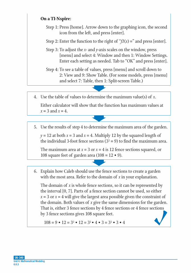
U6-340Unit 6: Mathematical Modeling6.8.3
On a TI-Nspire:
Step 1: Press [home]. Arrow down to the graphing icon, the second icon from the left, and press [enter].
Step 2: Enter the function to the right of “f1(x) =” and press [enter].
Step 3: To adjust the x- and y-axis scales on the window, press [menu] and select 4: Window and then 1: Window Settings. Enter each setting as needed. Tab to “OK” and press [enter].
Step 4: To see a table of values, press [menu] and scroll down to 2: View and 9: Show Table. (For some models, press [menu] and select 7: Table, then 1: Split-screen Table.)
4. Use the table of values to determine the maximum value(s) of x.
Either calculator will show that the function has maximum values at x = 3 and x = 4.
5. Use the results of step 4 to determine the maximum area of the garden.
y = 12 at both x = 3 and x = 4. Multiply 12 by the squared length of the individual 3-foot fence sections (32 = 9) to find the maximum area.
The maximum area at x = 3 or x = 4 is 12 fence sections squared, or 108 square feet of garden area (108 = 12 • 9).
6. Explain how Caleb should use the fence sections to create a garden with the most area. Refer to the domain of x in your explanation.
The domain of x is whole fence sections, so it can be represented by the interval [0, 7]. Parts of a fence section cannot be used, so either x = 3 or x = 4 will give the largest area possible given the constraint of the domain. Both values of x give the same dimensions for the garden. That is, either 3 fence sections by 4 fence sections or 4 fence sections by 3 fence sections gives 108 square feet.
108 = 9 • 12 = 32 • 12 = 32 • 4 • 3 = 32 • 3 • 4

U6-341Lesson 8: Geometric Modeling
6.8.3
Example 2
The city council is comparing two tank options for a new water tower: a cylindrical tank and a spherical tank. Both designs have a diameter of 20 meters. The cylindrical tank has a height of 12 meters. Both designs would cost $300 per square meter of surface area. The average monthly water bill is $100 per cubic meter of water, and either tank would hold enough water for 1 month. The city council decides to go with whichever tank will produce a net profit in its first month, assuming the tank’s full volume of water will be emptied completely (i.e., sold to customers) by the end of that month. Which tank will yield the desired profit?
1. Calculate the surface area of the spherical water tank using the formula A(r) = 4πr2.
The radius r of the spherical tank is 10 meters. Substitute this value into the formula to calculate the surface area.
A(r) = 4πr2 Formula for the surface area of a sphere
A(10) = 4π(10)2 Substitute 10 for r.
A(10) = 400π Simplify.
The surface area of the spherical water tank is 400π or about 1,257 square meters.
2. Use the surface area to calculate the cost of the spherical water tank.
The cost of the spherical water tank is $300 per square meter of surface area. Therefore, the cost to build the tank is 300 • 400π = 120,000π, or about $376,991.
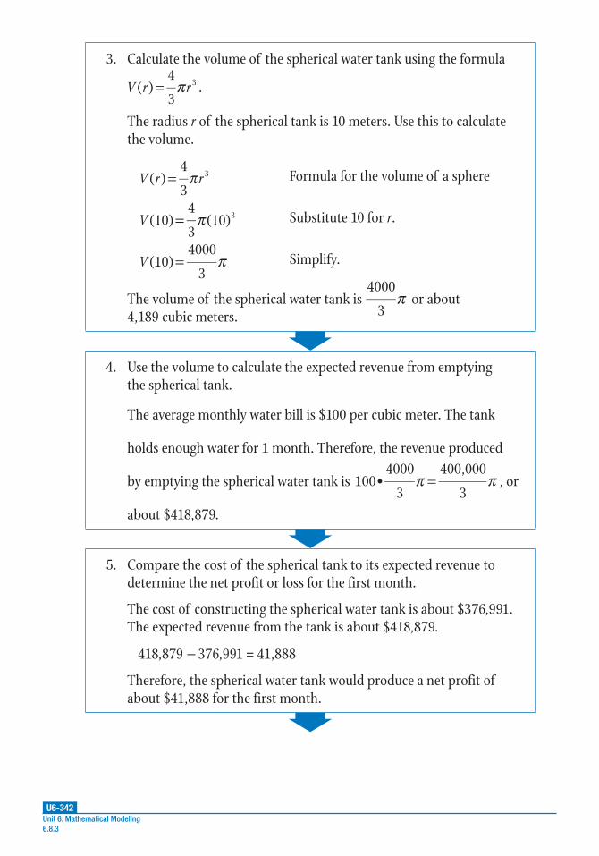
U6-342Unit 6: Mathematical Modeling6.8.3
3. Calculate the volume of the spherical water tank using the formula
V r r( )4
33π= .
The radius r of the spherical tank is 10 meters. Use this to calculate the volume.
V r r( )4
33π= Formula for the volume of a sphere
V (10)4
3(10)3π= Substitute 10 for r.
V (10)4000
3π= Simplify.
The volume of the spherical water tank is 4000
3π or about
4,189 cubic meters.
4. Use the volume to calculate the expected revenue from emptying the spherical tank.
The average monthly water bill is $100 per cubic meter. The tank
holds enough water for 1 month. Therefore, the revenue produced
by emptying the spherical water tank is 100•4000
3
400,000
3π π= , or
about $418,879.
5. Compare the cost of the spherical tank to its expected revenue to determine the net profit or loss for the first month.
The cost of constructing the spherical water tank is about $376,991. The expected revenue from the tank is about $418,879.
418,879 − 376,991 = 41,888
Therefore, the spherical water tank would produce a net profit of about $41,888 for the first month.

U6-343Lesson 8: Geometric Modeling
6.8.3
6. Calculate the surface area of the cylindrical water tank using the formula A(h, r) = 2πr2 + 2πrh.
The height of the tank is 12 meters and the radius is 10 meters. Use these values to calculate the surface area.
A(h, r) = 2πr2 + 2πrh Formula for the surface area of a cylinder with bases
A[(12), (10)] = 2π(10)2 + 2π(10)(12) Substitute 12 for h and 10 for r.
A(12, 10) = 440π Simplify.
The surface area of the cylindrical water tank is 440π or about 1,382 square meters.
7. Use the surface area to calculate the cost of the cylindrical water tank.
The cost of the cylindrical water tank is $300 per square meter. Therefore, the cost to build the tank is 300 • 440π = 132,000π, or about $414,690.
8. Calculate the volume of the cylindrical water tank using the formula V(h, r) = πrh.
The height of the tank is 12 meters and the radius is 10 meters. Use these values to calculate the volume.
V(h, r) = πr2h Formula for the volume of a cylinder
V[(12), (10)] = π(10)2(12) Substitute 12 for h and 10 for r.
V(12, 10) = 1200π Simplify.
The volume of the cylindrical water tank is 1200π or about 3,770 cubic meters.

U6-344Unit 6: Mathematical Modeling6.8.3
9. Use the volume to calculate the expected revenue from emptying the cylindrical tank.
The average water bill is $100 per cubic meter. Therefore, the revenue produced by emptying the cylindrical water tank is 100 • 1200π = 120,000π, or about $376,991.
10. Compare the cost of building the cylindrical water tank to its expected revenue to determine the net profit or loss for the first month.
The cost of constructing the cylindrical water tank is about $414,690. The expected revenue is about $376,991.
376,991 – 414,690 = –37,699
Therefore, the cylindrical water tank would produce a net loss of about $37,699 for the first month.
11. Compare the results for the two water tanks to determine which tank the city council will likely choose.
Based on the criteria used by the city council to compare the water tanks, the spherical water tank will be a more cost-effective tank to build because the spherical tank is expected to generate a profit in the first month (if completely emptied of water). The cylindrical tank, on the other hand, would generate a net loss.

U6-345Lesson 8: Geometric Modeling
6.8.3
Example 3
Autumn is an artist who specializes in decorative silk-screen panels. She recently bought several 60-centimeter and 80-centimeter wooden dowels to use as frames for the panels. Autumn decides to make several panels that are in the shape of quadrilaterals with two perpendicular diagonals made from the dowels. One diagonal will be 60 cm, and the other will be 80 cm. Autumn wants these panels to have the largest screen area possible, but she also needs to ensure the design makes the best use of her resources. What configuration of the two sizes of dowels should she use to realize this goal?
1. List all the possible configurations of the dowels in a table.
The diagonals can be perpendicular bisectors of each other, or one of the dowels can be a perpendicular bisector of the other dowel.
Case Description
IThe 60-cm dowel is a perpendicular bisector of the 80-cm dowel.
IIBoth dowels are perpendicular bisectors of each other.
IIIThe 80-cm dowel is a perpendicular bisector of the 60-cm dowel.
IVNeither dowel is a perpendicular bisector of the other.

U6-346Unit 6: Mathematical Modeling6.8.3
2. Sketch the four cases from step 1 and find the areas of the resulting figures.
The sketched figures are shown as follows, with each grid box
representing 10 cm. Notice that cases I−IV are each comprised of four
right triangles. Use this fact to find each area by adding the areas of
the triangles contained within each figure. (Recall that the formula for
the area of a triangle is A bh1
2= .)
I II
IIIIV
• Case I area: 2,400 cm2
• Case II area: 2,400 cm2
• Case III area: 2,400 cm2
• Case IV area: 2,400 cm2

U6-347Lesson 8: Geometric Modeling
6.8.3
3. Explain why the figures have equal areas.
Each panel has diagonal lengths of 60 cm and 80 cm. Visualize sliding the dowels within a panel’s frame, while still maintaining perpendicularity. Sliding the dowels changes the sizes of individual triangles within the panel, but does not change the total area enclosed within the panel.
4. Determine which configuration of dowels Autumn should use.
Since cases I−IV each use the same number of dowels and have the same area, Autumn could use any one of these configurations for her design.
Example 4
A mobile phone manufacturer has to upgrade the circuitry in one of its products. Currently, the voltage in the signal-capture circuit rises according to the exponential function model V(t) = 8(1 – e–at), in which a is a positive constant and the coefficient of t, the time in seconds, and V is the circuit voltage in volts. The graph shows how the voltage increases when a cell-phone tower signal is detected for a = 1.
0.5 1 1.5 2
t
10
9
8
7
6
5
4
3
2
1
0
V(t)
V(t) = 8(1 – e−at)
How will the function model have to be modified if the upgraded phone circuit has a voltage “rise time” that results in a circuit voltage of at least 7.9 volts in less than 1 second when a cell-phone tower signal is detected?

U6-348Unit 6: Mathematical Modeling6.8.3
1. Write an inequality using the function that reflects the necessary conditions for a faster rise time.
The voltage has to reach at least 7.9 volts in less than 1 second. Substituting V = 7.9 volts and t = 1 second in the function model gives 7.9 ≥ 8(1 – e–a).
2. Solve the resulting inequality.
7.9 ≥ 8(1 – e–a) Inequality from the previous step
7.9 ≥ 8 – 8e–a Distribute.
−0.1 ≥ –8e–a Isolate the exponential term.
0.0125 ≥ e–a Simplify.
−a ≤ ln (0.0125) Rewrite as a natural logarithm.
a ≥ 4.4 Use a calculator to simplify.
A value of a ≥ 4.4 will give a function that models a circuit that will reach a voltage of at least 7.9 volts in a rise time of 1 second.
3. Check the result of the previous step by substituting it into the original exponential function.
V(t) = 8(1 – e–at) General exponential function model
V(1) = 8[1 – e–(4.4)(1)] Substitute 1 for t and 4.4 for a.
V(1) = 8 – 8e–4.4 Distribute.
V(1) ≈ 8 – 8(0.012) Substitute the calculated value of e–4.4.
V(1) ≈ 7.9 Simplify.
The value a = 4.4 meets the conditions of the problem. Therefore, by modifying the function V(t) = 8(1 – e–at) so that a = 4.4, the upgraded phone circuit will achieve a voltage of at least 7.9 volts in less than 1 second.

U6-349
PRACTICE
UNIT 6 • MATHEMATICAL MODELINGLesson 8: Geometric Modeling
Lesson 8: Geometric Modeling6.8.3
A theremin is an electronic musical instrument played by passing one’s hands
near the instrument’s two antennas, which are connected to circuits. The function
model V I R fLfC
• 21
22
2
ππ
= + −
relates the current I and voltage V needed to
operate the instrument to three circuit components represented by C, L, and R. The
capacitance variable C is a measure of the electrical field produced by the instrument,
and f is the frequency of the alternating current in each circuit. The other component
values—I, L, R, and V—are constant. The movement of the user’s hands changes one
of the capacitance values and one of the frequency values; the other capacitance and
frequency values are fixed or hard-wired in the components of the instrument. Use this
information and the given facts that follow to complete problems 1–6.
Given:
• Audible music is produced when two such circuits produce signals with different frequencies (f1 and f2) that have different values of capacitance (C1 and C2).
• The absolute value of the difference of these frequencies, f f1 2− , is an audible frequency that ranges from about 20 cycles per second to around 20,000 cycles per second.
• Engineers who design the instruments have to select values of C1, C2, I, L, R, and V that produce the frequencies f1 and f2 that result in audible sounds.
1. Rewrite the function model so that I = 8 amperes and V = 24 volts, using C1 for the capacitance and f1 for the frequency. Then, rewrite the same function model beside the first model, using C2 for the capacitance and f2 for the frequency.
Practice 6.8.3: Design
continued
U6-350
PRACTICE
UNIT 6 • MATHEMATICAL MODELINGLesson 8: Geometric Modeling
Unit 6: Mathematical Modeling6.8.3
2. How can both functions be expressed so that the radical term is on one side of the equation and V divided by I is on the other?
3. How can both functions be expressed so that the terms with C1 and C2 are isolated on one side?
4. What is the result of subtracting the equation with C2 and f2 from the equation with C1 and f1?
5. What is the result of simplifying the answer to problem 4 so that f1 – f2 is on one side of the equation and the terms containing C1 and C2 are on the other side of the equation?
6. Assume that C1 and f1 are hard-wired into the circuitry and cannot be changed. What happens to the frequency difference f1 – f2 if C2 is increased by 50 percent?
continued
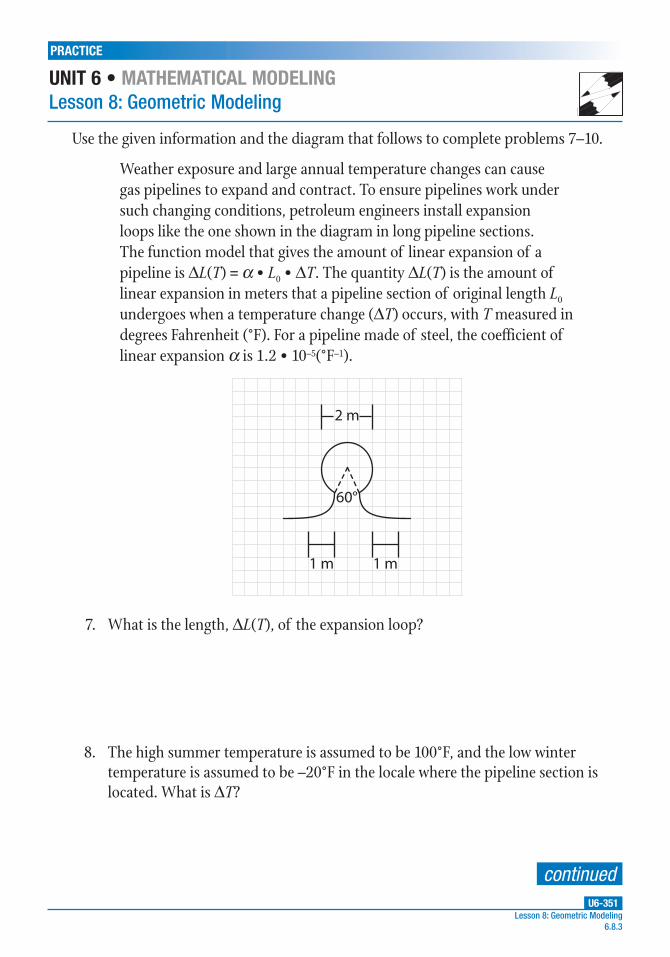
U6-351
PRACTICE
UNIT 6 • MATHEMATICAL MODELINGLesson 8: Geometric Modeling
Lesson 8: Geometric Modeling6.8.3
Use the given information and the diagram that follows to complete problems 7–10.
Weather exposure and large annual temperature changes can cause gas pipelines to expand and contract. To ensure pipelines work under such changing conditions, petroleum engineers install expansion loops like the one shown in the diagram in long pipeline sections. The function model that gives the amount of linear expansion of a pipeline is DL(T) = α • L0 • DT. The quantity DL(T) is the amount of linear expansion in meters that a pipeline section of original length L0 undergoes when a temperature change (DT) occurs, with T measured in degrees Fahrenheit (°F). For a pipeline made of steel, the coefficient of linear expansion α is 1.2 • 10–5(°F–1).
2 m
60°
1 m 1 m
7. What is the length, DL(T), of the expansion loop?
8. The high summer temperature is assumed to be 100°F, and the low winter temperature is assumed to be –20°F in the locale where the pipeline section is located. What is DT?
continued

U6-352
PRACTICE
UNIT 6 • MATHEMATICAL MODELINGLesson 8: Geometric Modeling
Unit 6: Mathematical Modeling6.8.3
9. Use the function model to find the original length, L0, of the pipeline section in which the loop has been installed.
10. The function model that describes how much force is needed to expand or
contract the pipeline is F rL
LA r( ) • ( )
0
γ=
. The variable γ is unique to steel
and has a value of 2 • 1011 Newtons per meter squared. The variable A(r) is the
cross section of the pipeline. Assume the pipeline radius is 1 meter. Use the
results of problems 7–9 to calculate the force required to produce the expansion
or contraction of the pipeline loop, DL(T).

AK-1Answer Key
Answer KeyLesson 1: Creating Equations
Practice 6.1.1: Creating Equations in One Variable, pp. U6-23–U6-24
1. Possiblelinearequationsinclude = +y x5
3
1
3, = −y x
7
5
1
5,andy=x+1.Thequadraticequationis
= − + +y x x2
15
23
15
3
52 .
2.
3. y=24.
5. Possibleequationsinclude y=–x+1, = − +y x5
4
3
4,and = − +y x
3
21 .
6.
7. = − − +y x x1
4
5
412
8.
9. d=20t +10
Practice 6.1.2: Creating Equations in Two Variables, pp. U6-42–U6-431. 576=16t2
2.
3. 2000+0.20x≥60004.
5. 4000=2000e0.0725t6.
7. f(0)=(0)3–(0)2–2(0) =0 f(2)=(2)3–(2)2–2(2)=0 f(–1)=(–1)3–(–1)2–2(–1)=08.
9. $32,500
Practice 6.1.3: Creating Exponential and Logarithmic Equations, pp. U6-54–U6-551. t≈38yearsold2.
3. A=9000(1+0.025)54.
5. 1.7grams6.
7. 44=–1.562+14.584lnt8.
9. 114,921=48,250e0.075t
Practice 6.1.4: Creating Rational, Radical, and Trigonometric Functions, pp. U6-74–U6-751. Thehorizontalasymptoteisaty=0becausethedegreeofthenumeratorislessthanthedegreeofthe
denominator.Asxapproachesinfinity,Capproaches0.Interpretation:Astimepasses,theconcentrationofthemedicationinthebloodstreamapproaches0.2.
3. Therearenoholesinthegraphofthefunction.4.
5. ThemonthspredictedtohavethemostsalesarethefirstJanuaryoftheforecastperiod(x=0)andthefollowingJanuary(x=12).Salesarepredictedtobeabout$118,500foreachmonth.
6.
7. P xx
x( )
360 56,000=
−
8.
9. sin2
2 sin2
ππ
π+
= ; sin
21
π=

AK-2Answer Key
Lesson 2: Piecewise, Step, and Absolute Value Functions
Practice 6.2.1: Piecewise Functions, pp. U6-86–U6-871. f(8)=3.22.
3. earnings:$4,000;transactionfeecharged:3%;totaltransactionfee:$1204.
5. 140units;220units;60units6.
7. f mm m
m m( )
300 0.25 ; 600
450 0.10( 600); 600=
+ ≤+ − >
;$640
200 400 600 800 1000 1200
x
800
750
700
650
600
550
500
450
400
350
300
250
200
150
100
50
0
y
8.
9. 2x+8
Practice 6.2.2: Step Functions, pp. U6-100–U6-1021. f(x)isaleastintegerfunction.
1 2 3 4 5 6 7 8
x
8
7
6
5
4
3
2
1
0
y
2.

AK-3Answer Key
3. f x
x
x
x
x
x
( )
2; 0 1
4; 1 2
6; 2 3
8; 3 4
10; 4 5
...
=
≤ <≤ <≤ <≤ <≤ <
Itcosts$10toparkfor4.5hours,whichis$2lessthanparkingfor5hoursatapriceof$12.
4.
5. f x
x
x
x
x
( )
3; 1 2
5; 2 4
8; 4 9
10; 9 12
=
− ≤ <≤ <≤ <≤ <
6.
7. (1.5,1),(2.5,2),and(3.5,3)8.
9. 2pounds
Practice 6.2.3: Absolute Value Functions, pp. U6-113–U6-1141. (2.5,3.5)2.
3. Thegraphoff(x)hasavertexof(0,0),whereasthegraphofg(x)hasavertexof(5,0).4.
5. Theequationofthegraphedfunctionisnot f x x( ) 2 10= − − − .Thegraphhasavertexat(–2,10),soh=–2andk=10.Inthegivenfunction,h=2andk=–10.Theactualequationofthegraphedfunctionisf x x( ) 2 10= − + + .6.
7. Thegraphwouldhavetoopenupwherea>0.8.
9. Thevertexoff(x)is(0,0),whereasthevertexforg(x)is(–2,0).10.
Lesson 3: Working with Constraint Equations and Inequalities
Practice 6.3.1: Creating Constraint Equations, pp. U6-126–U6-1271. 3h+2f =7.352.
3. If2t+4s=18.48,and2t=4s,eachindividualpairoftightscost$4.62andsockscost$2.31.4.
5. 3w+6r=126.
7. Graphsshouldfollowtheequationy =2–0.5x asshown;graphedpointsshouldmatchthoselistedfortheanswertoproblem6.
0.5 1 1.5 2 2.5 3 3.5 4
x
4
3.8
3.6
3.4
3.2
3
2.8
2.6
2.4
2.2
2
1.8
1.6
1.4
1.2
1
0.8
0.6
0.4
0.2
0
y
(1, 1.5)
(2, 1)
8.

AK-4Answer Key
9.
5,000 10,000 15,000 20,000 25,000 30,000
x
x + y = 27,000
0.10x + 0.12y = 2990
32,000
30,000
28,000
26,000
24,000
22,000
20,000
18,000
16,000
14,000
12,000
10,000
8,000
6,000
4,000
2,000
y
0
Practice 6.3.2: Creating Constraint Inequalities, pp. U6-136–U6-1371. 5j +p≤202.
3. Thesmallestamountoffruitshecanbuyis0,whichwouldallowhertopurchaseatmost20bagsofpopcorn.Thesmallestamountofpopcornbagsshecanbuyis0,whichwouldallowhertopurchaseatmost4bagsoffruit.4.
5.
50 60 70403020100
10
20
30
40
50
60
70
Playing
x
y
Feeding
6.
7. 60w+130r≥10008.
9. Sheneedstosellatleast2framedphotosandatleast5photoalbums.
Practice 6.3.3: Rearranging Formulas, pp. U6-155–U6-1561. P=Q2•R•t2
2.
3. [ ] [ ]=−
KaA
HA •10
10
pH
p or [ ] [ ]=− − KaA HA •10pH p
4.

AK-5Answer Key
5. Theescapevelocity vGM
rE=
+2
7500escapeactual
islessthantheescapevelocity vGM
rE=
−2
7500escapeactual
becausethe
denominatorsdifferbasedontheradiusinequality.6.
7. µ =t e
log2
•loggen8.
9. [A]•[B]<[AB];theproductoftheconcentrationsoftheelementsAandBislessthantheconcentrationofthecompoundAB.
Lesson 4: Transformations of Graphs
Practice 6.4.1: Transformations of Parent Graphs, pp. U6-173–U6-1751. f(x)=4(x–1);g(x)=4(x+1)2.
3. f(x)=2(4x);g(x)=–3(4x)4.
5. domain: (0, )∞ ;range: ( , )−∞ ∞6.
7. Ifthevalueofaisdoubledandbisincreasedby2,thenA(a,b)=π(2a–b–2)2.8.
9. ForapHrangeof(0,14),thedomainofcis(10–14);forapHrangeof(7,10),thedomainofcis(10–10,10–7).
Practice 6.4.2: Recognizing Odd and Even Functions, pp. U6-181–U6-1821. Foranevenfunction:Removex3andxtogivea(x)=x2+1.
Foranoddfunction:Removex2and1togivea(x)=x3+x.2.
3. Foranevenfunction: ( )1
2
2=+
c xx
x.
Foranoddfunction: ( )1 2=+
c xx
x.
4.
5. f(x)=0.5•cos0.2x;even6.
7. ( )1
=−
h xx
x;neither
8.
9. 1
2average 1 2( )= +I I I
Lesson 5: Comparing Properties Within and Between Functions
Practice 6.5.1: Reading and Identifying Key Features of Real-World Situation Graphs, pp. U6-207–U6-209
1. Therobotrepresentedbyf(t)takeslongertocompletetheinitialstepsthantherobotsrepresentedbyg(t)andh(t);therobotrepresentedbyh(t)completestheinitialstepsfastest,butitsrateofcompletionofthe10stepsislowerthanthatoftheothertworobots.2.
3. Inthereal-worldofmanufacturing,therewouldbeafinitetimetatwhichallthreerobotswouldcompletethe10CPU-fabricationstepssincea“step”mightbeassumedtobeapositivewholenumber;mathematically,noneofthethreerobotswouldevercompletethetenthstepifa“step”couldbeanypositivenumber;allthreewouldgetarbitrarilycloseto10,dependingonthevalueoft selected.4.
5. IfthefunctionN(t)givenintheproblemisused,they-axisscalewouldhavetobe0toatleast15.Thegraphrepresentstheexponentialfunctiongivenintheproblem,sovaluesofN(t)wouldincreasequicklyforinitialvaluesoftimebutwoulddeclineovertime.6.
7. Thedomainforthisfunctionmodelisarestricteddomainof13years;thedomainofthemathematicalsinefunctionisunrestricted.TherangeofH(t)isdefinedbytheconstant3.2andtheamplitudeof2.2,whichgivesarangeof[1,5.4].8.
9. approximately[0,1.9]
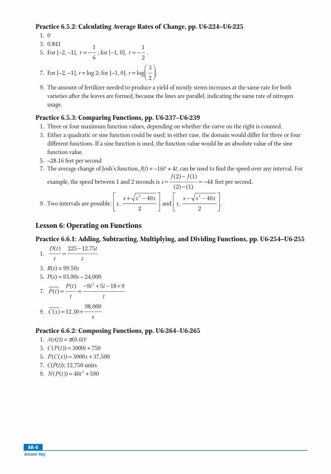
AK-6Answer Key
Practice 6.5.2: Calculating Average Rates of Change, pp. U6-224–U6-2251. 02.
3. 0.8414.
5. For[–2,–1], r1
6= − ;for[–1,0], r
1
2= − .
6.
7. For[–2,–1],r=log2;for[–1,0],r log3
2=
.
8.
9. Theamountoffertilizerneededtoproduceayieldofmostlystemsincreasesatthesamerateforbothvarietiesaftertheleavesareformed,becausethelinesareparallel,indicatingthesamerateofnitrogenusage.
Practice 6.5.3: Comparing Functions, pp. U6-237–U6-2391. Threeorfourmaximumfunctionvalues,dependingonwhetherthecurveontherightiscounted.2.
3. Eitheraquadraticorsinefunctioncouldbeused;ineithercase,thedomainwoulddifferforthreeorfourdifferentfunctions.Ifasinefunctionisused,thefunctionvaluewouldbeanabsolutevalueofthesinefunctionvalue.4.
5. –28.16feetpersecond6.
7. TheaveragechangeofJosh’sfunction,J(t)=–16t2+4t,canbeusedtofindthespeedoveranyinterval.For
example,thespeedbetween1and2secondsissJ J(2) (1)
(2) (1)44=
−−
= − feetpersecond.8.
9. Twointervalsarepossible: xx x x
,40
2
2+ −
and x
x x x,
40
2
2− −
.
Lesson 6: Operating on Functions
Practice 6.6.1: Adding, Subtracting, Multiplying, and Dividing Functions, pp. U6-254–U6-255
1. D t
t
t
t
( ) 225 12.75=
−
2.
3. R(x)=99.50x4.
5. P(x)=93.90x–24,0006.
7. P tP t
t
t t
t( )
( ) 9 5 18 92
= =− + − +
8.
9. C xx
( ) 12.3098,000
= +
Practice 6.6.2: Composing Functions, pp. U6-264–U6-2651. A(r(t))=π(0.6t)2
2.
3. C P t t( ( )) 3000 750= +4.
5. P C x x( ( )) 3000 37,500= +6.
7. C(P(t));12,750units8.
9. N P t t( ( )) 40 5902= +
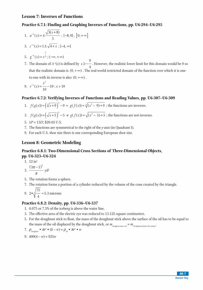
AK-7Answer Key
Lesson 7: Inverses of Functions
Practice 6.7.1: Finding and Graphing Inverses of Functions, pp. U6-294–U6-295
1. a xx
( )3( 8)
31 = ±
+− ; [ 8, 0]− , 0,[ ]+∞2.
3. c x x( ) 1 41 = ± +− ;[–4,∞]4.
5. g x x( ) ; ( , )13
4= −∞ +∞−6.
7. Thedomainof A–1(x)isdefinedby x9
4≥− .However,therealisticlowerlimitforthisdomainwouldbe0so
thattherealisticdomainis (0, )+∞ .Thereal-worldrestricteddomainofthefunctionoverwhichitisone-
to-onewithitsinverseisalso (0, )+∞ .8.
9. v xx
( )10
1012
= −− ;x>10
Practice 6.7.2: Verifying Inverses of Functions and Reading Values, pp. U6-307–U6-309
1. f g x x( ( )) 9 933( )= + − = g f x x( ( )) ( – 9) 933= + ;thefunctionsareinverses.
2.
3. f g x x( ( )) 5 52( )= + − ≠ g f x x( ( )) ( – 5) 52= + ;thefunctionsarenotinverses.
4.
5. 1P=13D;$20.02U.S.6.
7. Thefunctionsaresymmetricaltotherightofthey-axis(inQuadrantI).8.
9. ForeachU.S.shoesizethereisonecorrespondingEuropeanshoesize.
Lesson 8: Geometric Modeling
Practice 6.8.1: Two-Dimensional Cross Sections of Three-Dimensional Objects, pp. U6-323–U6-324
1. 12in2
2.
3.3 1
2ππ
( )−yd2
4.
5. Therotationformsasphere.6.
7. Therotationformsaportionofacylinderreducedbythevolumeoftheconecreatedbythetriangle.8.
9. 2•75
45.3 microns3 ≈
Practice 6.8.2: Density, pp. U6-336–U6-3371. 0.075or7.5%oftheicebergisabovethewaterline.2.
3. Theeffectiveareaoftheelectriceyewasreducedto13.125squarecentimeters.4.
5. Forthedoughnutsticktofloat,themassofthedoughnutstickabovethesurfaceoftheoilhastobeequaltothemassoftheoildisplacedbythedoughnutstick,orm
doughnutaboveoil=m
oildisplacedbelowthesurface.6.
7. ρdoughnut
•πr2•(h–w)=ρoil
•πr2•w8.
9. 400(4–w)=925w

AK-8Answer Key
Practice 6.8.3: Design, pp. U6-349–U6-352
1. 24 8• 21
22
11 1
2
R f Lf C
ππ
= + −
;24 8• 21
22
22 2
2
R f Lf C
ππ
= + −
2.
3. 1
22 9
1 11
2
f Cf L R
ππ= − − ;
1
22 9
2 22
2
f Cf L R
ππ= − −
4.
5.
1
2
1
22 ( )
1
4
1 11 1 2 2
1 2
21 1 2 2
1 2
f C f CL f f
L f C f Cf f
π ππ
π
− = −
−
= −
6.
7. 8
3
πorabout8.4meters
8.
9. 5,820meters