wall resolved large eddy simulation of a flow …

WALL RESOLVED LARGE EDDY

SIMULATION OF A FLOW THROUGH

A SQUARE-EDGED ORIFICE IN A

ROUND PIPE AT RE=25000

Code_Saturne User Meeting 2016

1st April, 2016

Sofiane Benhamadouche, Mario Arenas, Wadih Malouf

EDF R&D, Chatou, France

[email protected]

| 2

“80 PERCENT OF FLOW MEASUREMENT IN

FRENCH NPP USE DIFFERENTIAL

PRESSURE DEVICES … AND A BIG PART OF

THEM ARE ORIFICE PLATES”

Code_Saturne User Meeting - 01/04/2016

Nozzles (≈ 10%) Orifice plates (≈70%) Venturi (≈ 20%)

| 3

OUTLOOK


1. CONTEXT AND STRATEGY

2. TEST CASE

3. NUMERICAL SETUP

MESH GENERATION

NUMERICAL APPROACH

INLET BOUNDARY CONDITION

4. SENSITIVITY STUDIES

STATISTICS

SUB-GRID SCALE MODEL

5. COMPARISONS WITH EXPERIMENTAL DATA

LOCAL STATISTICS

RECIRCULATION ZONE

DISCHARGE AND PRESSURE LOSS COEFFICIENTS

6. CONCLUSIONS AND PERSPECTIVES

| 4

CONTEXT (1/2)


Orifice plate is a commonly used instrument for flow measurements in pipes, thanks to:

• Simplicity

• Standardized

• Installation and operation

not expensive

ISO 5167 /ISO TR12767

Relationship between ΔP and qm

Easily installed between flanges,

fabrication simple, no limitations on

the materials, line size and flowrate

Where:

C : discharge coefficient (calculated by ISO)

E: velocity of approach factor (known)

d : diameter of orifice (known)

ΔP: differential pressure (measured)

: density of the fluid (known)

Mass flowrate equation

| 5

CONTEXT (2/2)


The discharge coefficient (and its uncertainty) can be calculated if you know:

• Geometry

• Reynolds number

• Placement of pressure taps

• Fluids properties

• Straight lengths between orifice plates and fittings (bend, tee, reducer, etc.)

…but in some cases straight lengths are shorter than required and ISO 5167

cannot be used to predict the coefficient and the uncertainty.

What to do then?

Reader-Harris/Gallagher equation

Uncertainty of the

discharge coefficient C

ISO

5167-2

| 6

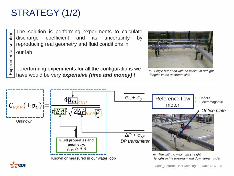
STRATEGY (1/2)

The solution is performing experiments to calculate

discharge coefficient and its uncertainty by

reproducing real geometry and fluid conditions in

our lab

…performing experiments for all the configurations we

have would be very expensive (time and money) !ex. Single 90° bend with no minimum straight

lengths in the upstream sideExp

erim

en

tal so

lutio

n

Fluid properties and

geometry:

ρ, µ, D, d, β

Orifice plate

DP transmitter

Reference flow

meter

qm + σqm

ΔP + σΔP

• Coriolis

• Electromagnetic


ex. Tee with no minimum straight

lengths in the upstream and downstream sidesKnown or measured in our water loop

Unknown

| 7

STRATEGY (2/2)


Validate the CFD calculations

Apply the methodology to an industrial problem

Apply the obtained

methodology for all such

configurations

Apply the obtained

methodology for all such devices

• Experiment of simple cases

• PIV, LDV (velocity)

• Multipoint pressure

measurements

• CFD simulations (RANS)

Hyb

rid

so

lutio

n (

exp

. / C

FD

)

• Experiment data for

Velocity and pressure

• CFD simulations (RANS)

• Sensitivity tests

We’re here

From the lab to the industry…

• Nozzles

• Venturi tubes

• Multi-hole orifice plate

• In the scope of ISO

• Beyond the scope

of ISO

1D 0.5D

Orifice plate

Fluid properties and

geometry:

ρ, µ, D, d, β

| 8

TEST CASE


Features of Shan et al. case

• Square-edged orifice

• Round pipe

• Standard water

• Smooth pipe wall

• Re = 25000

• Velocity fields measurement (PIV)

…but a doubt arose about

experimental data uncertainties…

Solution

Using Large Eddy Simulations to:

• Better understand flow

• Predictions of pressure losses and C𝐸 = 1/ 1 − 𝛽4

| 9

NUMERICAL SETUP (1/3)


Mesh generation

Features of mesh

• ICEM CFD v14.0

• 55 million cells

• Structured and refined near the orifice

• Conformal throughout the domain

• Solution is resolved beyond the Taylor micro-scale

(using a RANS computation, on uses 15𝑘/ )

• Wall shear velocity u* = 0.025 m/s

• Distance 𝑦+ is kept below 1 almost everywhere

• x+max=40, r+max=10, r+max=12

| 10



• In-house open-source EDF CFD tool (www.code-saturne.org)

• The LES capabilities of Code_Saturne have been validated on various

academic and industrial cases

• Temporal discretization for the LES is second order in time with linearized

convection (Crank Nicolson and Adams Bashforth), CFL<1 almost everyt

• Spatial discretization is a pure second order central difference scheme

• Sub-grid scale models used are the Dynamic Smagorinsky (no negative

values, Csmax=0.065), the standard Smagorinsky (Cs=0.065) and no SGS

model

• High Performance Computing (HPC): Blue Gene/Q supercomputer, using

a total of 256 nodes (4,096 processors - Power BQC 16C 1.6GHz), 2.2 s

per time step

• Post-processing: Ensight, Matlab

http://www.code-saturne.org/

| 11Code_Saturne User Meeting - 01/04/2016


Inlet boundary condition

• The inlet is located 18D upstream

• The inlet profile is simulated through a recycling method

Pressure Loss and discharge coefficients

• Discharge: p 1D upstream of the orifice and 0.5D downstream (from the upstream face of

the contraction)

• Pressure Loss: p 2D upstream of the orifice and 6D downstream

| 12

SENSITIVITY STUDIES (1/2)


Statistics

Instantaneous azimuthal velocity field: the

structures are characteristic of a fully

developed turbulent flow in a pipe

The velocity, pressure and Reynolds

stresses are averaged in time:

• 8 flow-passes for dynamic Smagorinsky

(1.2 million time steps)

• 4.5 flow-passes for the other SGS models

| 14Code_Saturne User Meeting - 01/04/2016

SENSITIVITY STUDIES (2/2)

Sub-grid scale model

• No significant differences between the three different SGS models and similar results for Rii profiles

• The close resemblance between all three models demonstrates that the LES is well resolved

beyond the Taylor micro-scale, as the influence of the SGS model is almost negligible

Str

ea

mw

ise

ve

locity u

x

Ra

dia

l ve

locity u

r

The downstream recirculation

reattachment points are

determined as the point at which

the wall shear stress, 𝜏𝑤𝑎𝑙𝑙changes direction

| 15

COMPARISONS WITH EXPERIMENTAL DATA (1/3)


Local statistics

Norm

aliz

ed

str

eam

wis

e v

elo

city u

x

Norm

aliz

ed r

adia

l

velo

city u

r

Norm

aliz

ed

R11

• The centerline stream-wise velocity normalized

by the average velocity shows very similar

behavior between the PIV observations and LES

• The shapes of both the LES and PIV stream-wise

and radial velocity profiles provide a close match

• The results differ in two important zones: high

gradients of the velocity and near wall region

| 16



Recirculation zones

It is clear that the predicted reattachment points calculated with the same methodology using

PIV data and the LES are similar

FFP method

(Forward Flow Probability,

0.056R from the wall)

Stream-wise velocity zero-

crossing method (0.028R from

the wall)

PIV LES (zero

w)

Δ% PIV LES (D-S) Δ%

Primary

reattachment

3.64R 3.92R +7.7 3.62R 3.60R -0.55

Secondary

reattachment

- - 0.27R 0.34R 26

| 17



Pressure loss and discharge coefficients

• The results between the ISO standards and the LES are in very close agreement which serves

as further validation of the LES results

The discharge coefficient, 𝐶𝐷,𝐼𝑆𝑂 = 0.628

± 0.005 (0.8%) and the pressure loss

coefficient K𝑖𝑠𝑜 = 8.71 ± 0.07 (0.8%)

The discharge coefficient, 𝐶𝐷,LES = 0.632

and the pressure loss coefficient KLES =

8.64 (Idel’cik gives 8.61)

| 18

CONCLUSIONS AND PERSPECTIVES (3/3)


• This study demonstrates that a very fine wall-resolved LES with a dynamic Smagorinsky

SGS can accurately and precisely simulate a single phase flow through a square-edged

orifice plate.

• A sensitivity study shows that the effect of the SGS model and pressure-velocity coupling

is negligible

• The LES shows excellent agreement with the velocity from the experimental data

• The pressure loss coefficient and discharge coefficient are also shown to be in agreement

with the predictions of ISO 5167-2

• The results from this simulation can be used to validate other simulation techniques such

as RANS approaches

Next step…

Validation of RANS results by LES

ones seems to be possible when no

experimental data are available

What’s the best turbulence model?

And then…

Apply the methodology to an industrial

problem (second step of hybrid strategy)

Thanks

wall resolved large eddy simulation of a flow …

Documents