wanted!: open m&s standards and technologies for the smart grid - introducing rapid and ipsl:...
TRANSCRIPT
Wanted!: Open M&S Standards and Technologies for the Smart Grid
Luigi Vanfretti, PhDhttp://www.vanfretti.com
North America Modelica Users’ Group ConferenceUniversity of Connecticut, Storrs, USA
Nov 12, 2015
[email protected] Professor, Docent
Electric Power Systems Dept.KTH
Stockholm, Sweden
[email protected] Advisor
Research and Development Division Statnett SFOslo, Norway
Introducing RaPId and iPSLOSS Tools for Power System Model, Simulation and Model Validation from the FP7 iTesla Project

Outline• Background
– Modeling, Simulation and Model Validation Needs in Power Systems
• The iTesla Toolbox – Toolbox Architecture and Services– Need for Time-‐Domain Simulation Engines
• iTesla iPSL– A Modelica Library for Phasor Time-‐Domain Power System Modeling and Simulation– Software-‐to-‐Software Validation with Domain-‐Specific Tools
• iTesla RaPId– Model validation software architecture based using Modelica tools and FMI Technologies– The Rapid Parameter Identification Toolbox (RaPId)
• Using the FMI for Power System Simulation using xengen and iPSL
• Conclussions

MODELING AND SIMULATIONHow to anticipate problems during operation?
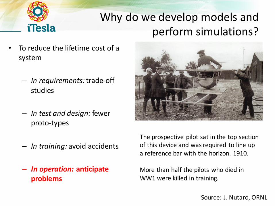
Why do we develop models and perform simulations?
• To reduce the lifetime cost of a system
– In requirements: trade-‐off studies
– In test and design: fewer proto-‐types
– In training: avoid accidents
– In operation: anticipate problems
The prospective pilot sat in the top section of this device and was required to line up a reference bar with the horizon. 1910.
More than half the pilots who died in WW1 were killed in training.
Source: J. Nutaro, ORNL
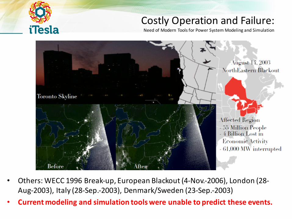
• Others: WECC 1996 Break-‐up, European Blackout (4-‐Nov.-‐2006), London (28-‐Aug-‐2003), Italy (28-‐Sep.-‐2003), Denmark/Sweden (23-‐Sep.-‐2003)
• Current modeling and simulation tools were unable to predict these events.
Costly Operation and Failure:Need of Modern Tools for Power System Modeling and Simulation
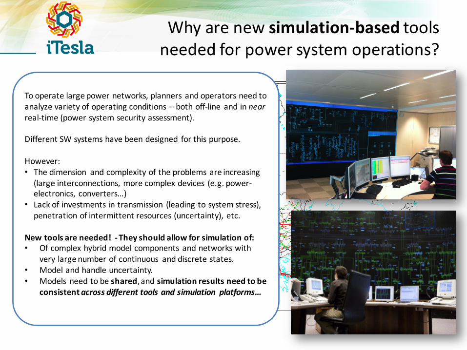
Why are new simulation-‐based tools needed for power system operations?
To operate large power networks, planners and operators need to analyze variety of operating conditions – both off-‐line and in nearreal-‐time (power system security assessment).
Different SW systems have been designed for this purpose.
However:• The dimension and complexity of the problems are increasing (large interconnections, more complex devices (e.g. power-‐electronics, converters…)
• Lack of investments in transmission (leading to system stress), penetration of intermittent resources (uncertainty), etc.
New tools are needed! -‐ They should allow for simulation of:• Of complex hybrid model components and networks with
very large number of continuous and discrete states.• Model and handle uncertainty.• Models need to be shared, and simulation results need to be
consistentacross different tools and simulation platforms…

Common Architecture of « most » Available Power System Security Assessment Tools
Online
Data acquisition and storage
Merging module
Contingency screening (static power flow)
Synthesis of recommendationsfor the operator
External data (forecasts and snapshots)
“Static power flow model”
That means no (dynamic) time-‐domain simulation is performed.
The idea is to predict the future behavior under a given ‘contingency’ or set of contingencies.
BUT, the model has no dynamics – only nonlinear algebraic equations.
Computations made on the power system model are based on a “power flow” formulation.
Result : difficult to predict the impact of a contingency without considering system dynamics!

iTesla Toolbox Architecture
How to Validate Dynamic Models?
Online Offline
Sampling of stochastic variables
Elaboration of starting network
states
Impact Analysis(time domainsimulations)
Data mining on the results of simulation
Data acquisition and storage
Merging module
Contingency screening (several stages)
Time domain simulations
Computation of security rules
Synthesis of recommendations for the operator
External data (forecasts and snapshots)
Improvements of defence and
restoration plans
Offline validation of dynamic models
Where are Dynamic Models used in
iTesla?

What do we want to simulate?Power system dynamics
10-‐7 10-‐6 10-‐5 10-‐4 10-‐3 10-‐2 10-‐1 1 10 102 103 104
Lightning
Line switching
SubSynchronous Resonances, transformer energizations…
Transient stability
Long term dynamics
Daily load following
seconds
Electromechanical Transients
Electromagnetic Transients
Quasi-‐Steady State Dynamics
Phasor Time-‐Domain Simulation

Example of Power System Dynamics in Europe February 19th 2011
49.85
49.9
49.95
50
50.05
50.1
50.15
08:08:00 08:08:10 08:08:20 08:08:30 08:08:40 08:08:50 08:09:00 08:09:10 08:09:20 08:09:30 08:09:40 08:09:50 08:10:00
f [Hz]
20110219_0755-0825
Freq. Mettlen Freq. Brindisi Freq. Wien Freq. Kassoe
SynchornizedPhasorMeasurement Data

Hypotheses& Simplifications
PhysicalSystem
Models
Equations
AnalyticalMethods
Analyses
SpecializedM&S
Platform
PhysicalSystem
User DefinedModels in PlatformSpecific Language
Models withFixed
Equations
Available(Limited)NumericalAlgorithms
Analyses
NumericalMethods
Modeling and SimulationGeneral Approach vs Power System Approach
Hypotheses(assumptions)
Simplifications(approximations)
General Approach Power Systems Approach
Closed-‐FormSolution
NumericalSolution
User: Modeler and Analyst Duality
SpecializedModeler Familiarwiththe Domain Specific Platform
SpecializedAnalystFamiliarwiththe Domain
Specific Platform
FixedModel is ”interlaced” withone specific solver

We will separate the algebraic equations into two sets:
(1.) Is the part which governs how dynamic models will evolve, since they depend on both and , e.g. generators and their control systems.(2.) Is the network model, consisting of transmission lines and other passive components which only depends on algebraic variables,
Power System Simulation ApproachSeparation into Network and Dynamic Component Models.
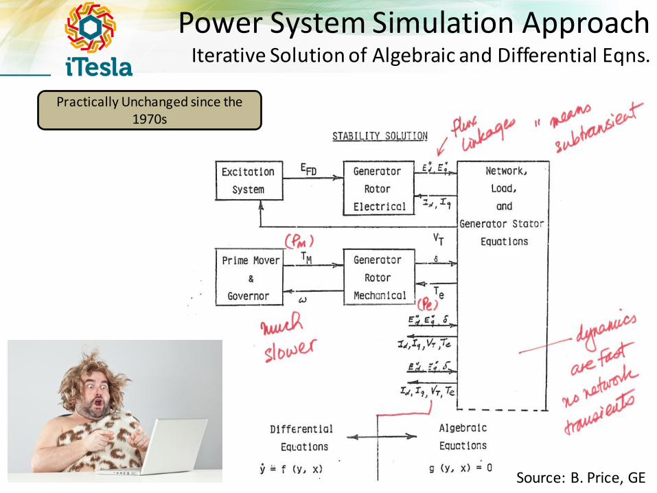
Power System Simulation Approach Iterative Solution of Algebraic and Differential Eqns.
Practically Unchanged since the 1970s
Source: B. Price, GE
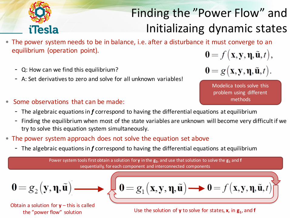
• The power system needs to be in balance, i.e. after a disturbance it must converge to an equilibrium (operation point).
- Q: How can we find this equilibrium? - A: Set derivatives to zero and solve for all unknown variables!
• Some observations that can be made:- The algebraic equations in f correspond to having the differential equations at equilibrium - Finding the equilibrium when most of the state variables are unknown will become very difficult if we
try to solve this equation system simultaneously.• The power system approach does not solve the equation set above- The algebraic equations in f correspond to having the differential equations at equilibrium
Finding the ”Power Flow” and Initializaing dynamic states
Modelica tools solve this problem using different
methods
Power system tools first obtain a solution for y in the g2, and use that solution to solve the g1 and fsequentially, for each component and interconnected components
Obtain a solution for y – this is calledthe ”power flow” solution Use the solution of y to solve for states, x, in g1, and f
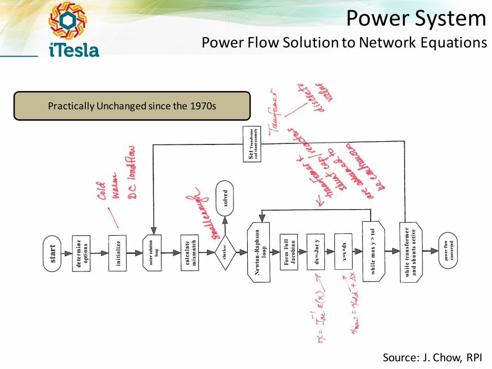
Power System Power Flow Solution to Network Equations
Practically unchanged since the
1970sPractically Unchanged since the 1970s
Source: J. Chow, RPI

Initialization of Algebraic and Dynamic Equations
Example Initial Equations for an Excitation System Model – IEEET2
Initial Equations
Sequential Solution of Initial Equations of Coupled Dynamic Components
Source: F. Milano

Power Systems Status Quo of Modeling and Simulation Tools
10-‐7 10-‐6 10-‐5 10-‐4 10-‐3 10-‐2 10-‐1 1 10 102 103 104
Lightning
Line switching
SubSynchronous Resonances, transformer energizations…
Transient stability
Long term dynamics
Daily load following
seconds
Phasor Time-‐Domain Simulation
PSS/EStatus Quo:Multiple simulation tools, with their own interpretation of different model features and data “format”.Implications of the Status Quo:-‐ Dynamic models can rarely be shared in a
straightforward manner without loss of information on power system dynamics (parameter not equal to equations, block diagrams not equal to equations)!
-‐ Simulations are inconsistent without drastic and specialized human intervention.
Beyond general descriptions and parameter values, a common and unified modeling language would require a formal mathematical description of the models – but this is not the practice to date.
These are key drawbacks of today’s tools for tackling pan-‐European problems.

UNAMBIGUOUS MODELING AND SIMULATION FOR POWER SYSTEMS
Modeling and Simulation using Modelica

Power System Modelinglimitations, inconsistency and consequences
• Causal Modeling:– Most components are defined using causal block diagram definitions.– User defined modeling by scripting or GUIs is sometimes available (casual)
• Model sharing:– Parameters for black-‐box definitions are shared in a specific “data format”– For large systems, this requires “filters” for translation into the internal data format of each program
• Modeling inconsistency:– For (standardized casual) models there is no guarantee that the model definition is implemented “exactly” in the
same way in different SW– This is even the case with CIM (Common Information Model) dynamics, where no formal equations are defined,
instead a block diagram definition is provided.– User defined models and proprietary models can’t be represented without complete re-‐implementation in each
platform
• Modeling limitations:– Most SWs make no difference between “model” and “solver”, and in many cases the model is somehow
implanted within the solver (inline integration, eg. Euler or trapezoidal solution in transient stability simulation)
• Consequence: – It is almost impossible to have the same model in different simulation platforms.– This requires usually to re-‐implement the whole model from scratch (or parts of it) or to spend a lot of time “re-‐
tuning” parameters.
This is very costly!
An equation based modeling language can help in avoiding all of
these issues!

iTesla Power Systems Modelica Library
• Power Systems Library:– The Power Systems library developed using
as reference domain specific software tools (e.g. PSS/E, Eurostag, PSAT and others)
– The library is being tested in several Modelica supporting software: OpenModelica, Dymola, SystemModeler
– Components and systems are validated against proprietary tools and one OSS tool used in power systems (domain specific)
• New components and time-‐driven events are being added to this library in order to simulate new systems.– PSS/E (proprietary tool) equivalents of
different components are now available and being validated.
– Automatic translator from domain specific tools to Modelica will use this library’s classes to build specific power system network models is being developed.
Model Editing in OpenModelica
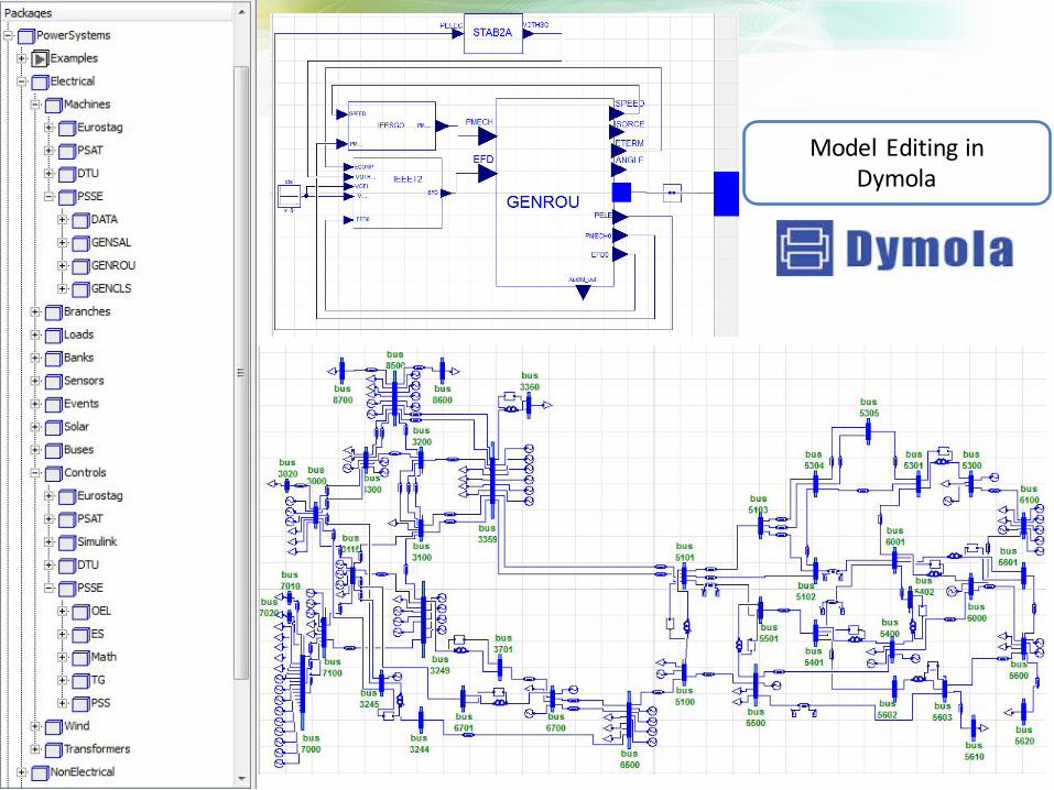
Model Editing inDymola

SW-‐to-‐SW Validation of Models in Domain Specific Tools used by TSOs
• Includes dynamicequations for– Eletrocmagnetic dynamics– Motion dynamics– Saturation
• Boundary equations– Change of coordinates from the abc
to dq0 frame– Stator voltage equations
• Initial condition (guess) values for the initializationproblem areextracted from a steady-‐statesolution
Validation of a PSS/E Model: Genrou

Typical SW-‐to-‐SW Validation TestsModelica vs. PSS/E
• Basic Test Network
• Perturbation scenarios

• Set-‐up a model in each tool with the simulation scenario configured
• In the case of Modelica, the simulation configuration can be done within the model
• In the case of PSS/E, a Python script is created to perform the same test.
• Sample Test:1. Running under steady state for 2s.2. Vary the system load with constant
P/Q ratio.3. After 0.1s later, the load was
restored to its original value .4. Run simulation to 10s.5. Apply three phase to ground fault.6. 0.15s later clear fault by tripping
the line.7. Run simulation until 20s.
Experiment Set-‐Up of SW-‐to-‐SWValidation Tests and Results
Modelica
PSS/E
Python

SW-‐to-‐SW Validation ofLarger Grid Models
Original “Nordic 44” Model in PSS/E
Line opening
Bus voltages
Implemented “Nordic 44” Model in Modelica

SW-‐to-‐SW Validation -‐ Nordic 44 GridSample Simulation Experiment
PSS/E Dymola
DELT (simulation time step): 0.01
Number of intervals: 1500 (number chosen in order to have almost the same simulation points as PSSE)
Network solution tolerance:0.0001
Algorithm: Rkfix2
Tolerance: 0.0001
Fixed Integrator Step: 0.01
Simulation time 0-‐10 sec
Type and location of fault Line opening between buses 5304-‐5305
Fault time t=2 sec
Simulation Configuration in PSS/E and Dymola
Simulation Configuration in PSS/E and Dymola
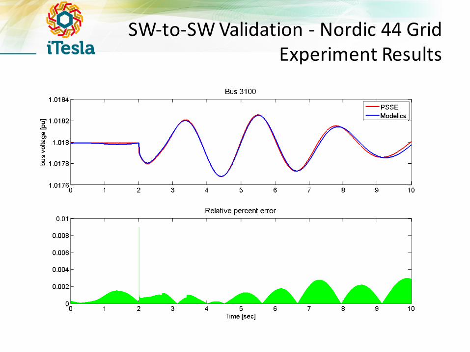
SW-‐to-‐SW Validation -‐ Nordic 44 GridExperiment Results
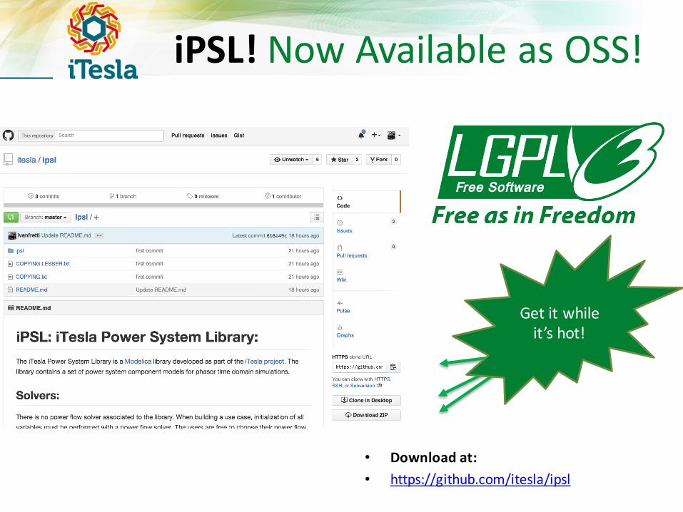
iPSL! Now Available as OSS!
• Download at:• https://github.com/itesla/ipsl
Get it while it’s hot!
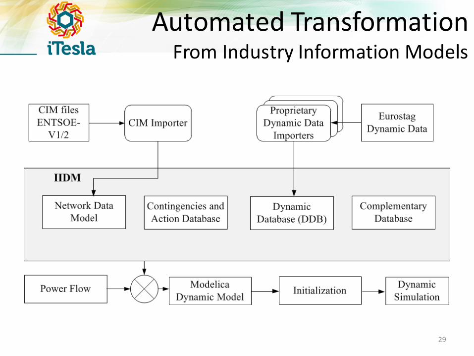
Automated TransformationFrom Industry Information Models
29

Generating Modelica Models: Automatic Transformation from Eurostagand PSSE
model Nordic32parameter Real SNREF = 100.0;PowerSystems.Connectors.ImPin omegaRef;// BUSES// LINES// FIXED TRANSFORMERS// LOADS// CAPACITORS// GENERATORS// REGULATORS// EVENTPowerSystems.Electrical.Events.PwFault pwFault(R = 0.1, X = 0.1, t1 = 20, t2 = 150);equationomegaRef = sum of omega from all generatorsconnect(pwGeneratorM2S.omegaRef, omegaRef);// Connecting REGULATORS and MACHINESconnect(htgpsat3.pin_CM,pwGeneratorM2S.pin_CM);// Connecting LINESconnect(bus.p, pwLine.p);// COUPLING DEVICES// Connecting LOADSconnect(bus.p, pwLoadPQ.p);// Connecting Capacitorsconnect(bus.p, pwCapacitorBank.p));// Connecting GENERATORSconnect(bus.p, pwGeneratorM2S.sortie);…// Connecting FIXED TRANSFORMERSconnect(bus.p, pwTransformer.p);…//Connecting FAULTconnect(bus.p, pwFault.p);end Nordic32;
model Nordic44parameter Real SNREF = 100.0;// BUSES// TAP CHANGER TRANSFORMERS// LINES// LOADS// CAPACITORS// GENERATORS// REGULATORS// EVENT:FAULTPowerSystems.Electrical.Events.PwFault_fault(X = 0.5, R = 0.5, t1 = 20, t2 = 100);equation// Connecting REGULATORS and MACHINESconnect(stab2a.PELEC, gENROU.PELEC);…// Connecting REGULATORS and REGULATORSconnect(stab2a.VOTHSG, ieeet2.VOTHSG);…// Connecting REGULATORS and CONSTANTSconnect(ieeet2.VOEL, const.y);…// Connecting LINESconnect(_bus.p, pwLine_2.p);…// COUPLING DEVICES// Connecting LOADSconnect(bus.p, pwLoadVoltageDependence.p);…// Connecting CapacitorsConnect(bus.p, pwCapacitorBank.p);…// Connecting GENERATORSconnect(bus.p, gENROU.p);…// Connecting DETAILED TRANSFORMERSconnect(bus.p, pwPhaseTransformer.p);//Connecting FAULTconnect(bus.p, _fault.p);end Nordic44;
30
From EurostagFrom PSS/E

Validation Result (1/2)• Nordic 32 – Eurostag to Modelica
31
Test System Variable RMSE MSENordic 32 V2032 9.2378e-04 8.53382e-07

Validation Result (2/2)• Nordic 44 – PSS/E to Modelica
32
Test System Variable RMSE MSENordic 44 V3020 9.0215e-05 8.13877e-09

Reminder: models are used as a key enabler of the iTesla Toolbox!
Sampling of stochastic variables
Elaboration of starting network
states
Impact Analysis(time domainsimulations)
Data mining on the results of simulation
Data acquisition and storage
Merging module
Contingency screening (several stages)
Time domainsimulations
Computation of security rules
Synthesis of recommendationsfor the operator
External data (forecasts and snapshots)
Improvements of defence and
restoration plans
Offline validation of dynamic models
Data management
Data mining services
Dynamic simulation Optimizers Graphical
interfaces
Modelica use fortime-‐domain simulation
THE RAPID TOOLBOXA model validation, identification and parameter estimation SW
Modeling, Simulation Tools and Model Validation
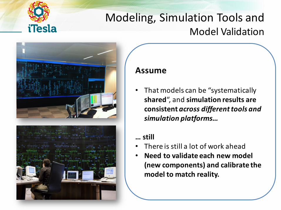
Assume
• That models can be “systematically shared“, and simulation results are consistentacross different tools and simulation platforms…
… still• There is still a lot of work ahead• Need to validate each new model
(new components) and calibrate the model to match reality.
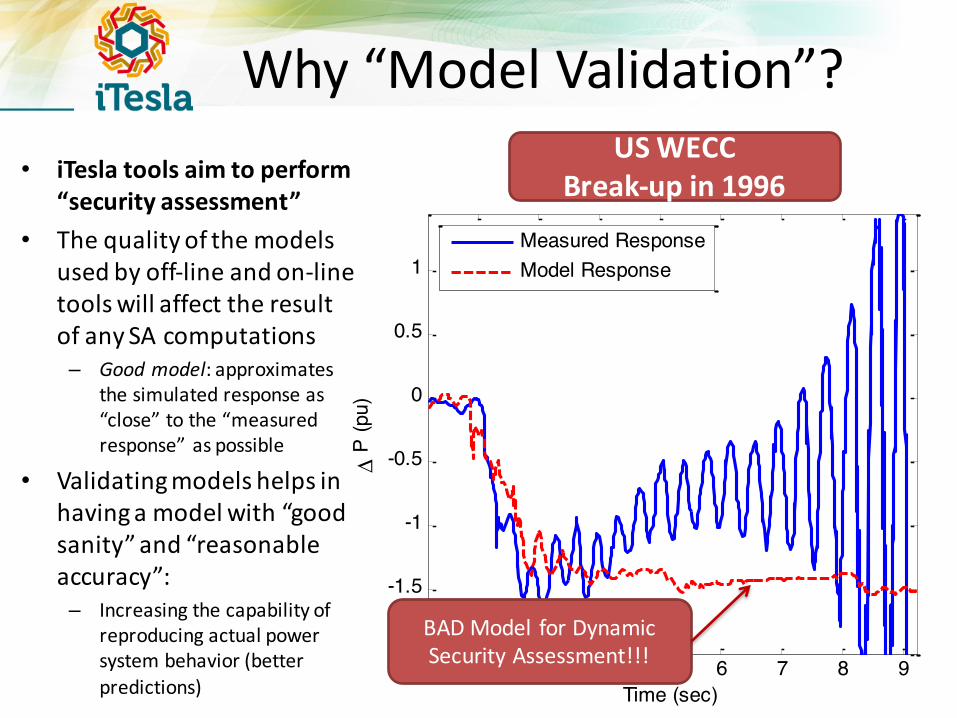
Why “Model Validation”?• iTesla tools aim to perform
“security assessment”• The quality of the models
used by off-‐line and on-‐line tools will affect the result of any SA computations– Good model: approximates
the simulated response as “close” to the “measured response” as possible
• Validating models helps in having a model with “good sanity” and “reasonable accuracy”: – Increasing the capability of
reproducing actual power system behavior (better predictions)
2 3 4 5 6 7 8 9-2
-1.5
-1
-0.5
0
0.5
1
Δ P
(pu)
Time (sec)
Measured ResponseModel Response
US WECC Break-‐up in 1996
BAD Model for Dynamic Security Assessment!!!
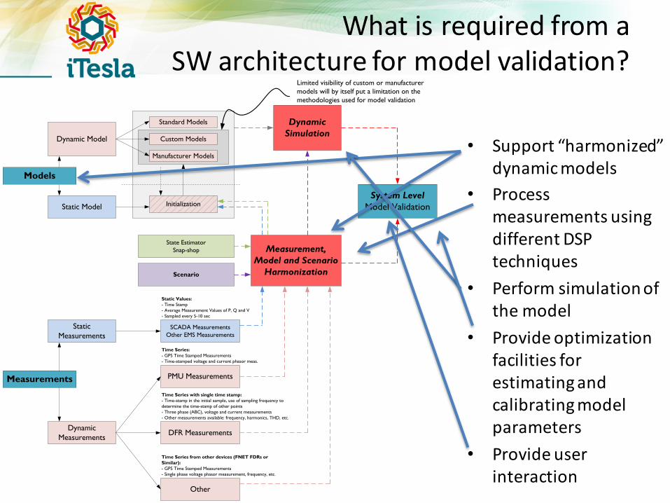
What is required from a SW architecture for model validation?
Models
Static Model
Standard Models
Custom Models
Manufacturer Models
System LevelModel Validation
Measurements
Static Measurements
Dynamic Measurements
PMU Measurements
DFR Measurements
Other
Measurement, Model and Scenario
Harmonization
Dynamic Model
SCADA MeasurementsOther EMS Measurements
Static Values:- Time Stamp- Average Measurement Values of P, Q and V- Sampled every 5-10 sec
Time Series:- GPS Time Stamped Measurements- Time-stamped voltage and current phasor meas.
Time Series with single time stamp:- Time-stamp in the initial sample, use of sampling frequency to determine the time-stamp of other points- Three phase (ABC), voltage and current measurements- Other measurements available: frequency, harmonics, THD, etc.
Time Series from other devices (FNET FDRs or Similar):- GPS Time Stamped Measurements- Single phase voltage phasor measurement, frequency, etc.
Scenario
Initialization
State Estimator Snap-shop
DynamicSimulation
Limited visibility of custom or manufacturer models will by itself put a limitation on the methodologies used for model validation
• Support “harmonized” dynamic models
• Process measurements using different DSP techniques
• Perform simulation of the model
• Provide optimization facilities for estimating and calibrating model parameters
• Provide user interaction
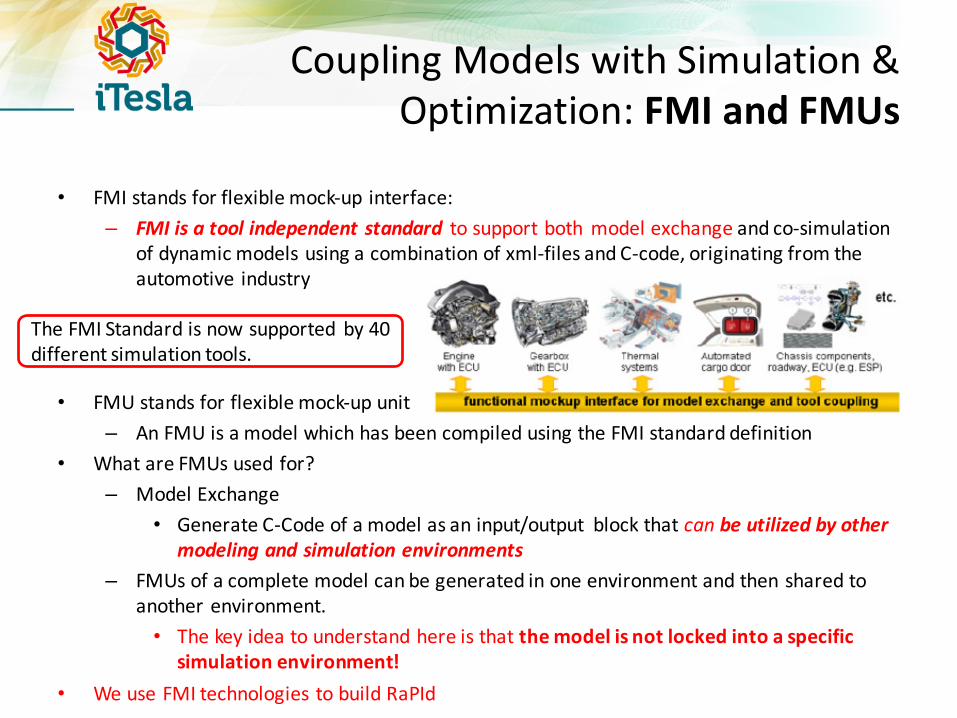
Coupling Models with Simulation & Optimization: FMI and FMUs
• FMI stands for flexible mock-‐up interface:– FMI is a tool independent standard to support both model exchange and co-‐simulation
of dynamic models using a combination of xml-‐files and C-‐code, originating from the automotive industry
• FMU stands for flexible mock-‐up unit– An FMU is a model which has been compiled using the FMI standard definition
• What are FMUs used for?– Model Exchange
• Generate C-‐Code of a model as an input/output block that can be utilized by other modeling and simulation environments
– FMUs of a complete model can be generated in one environment and then shared to another environment.• The key idea to understand here is that the model is not locked into a specific
simulation environment!• We use FMI technologies to build RaPId
The FMI Standard is now supported by 40 different simulation tools.
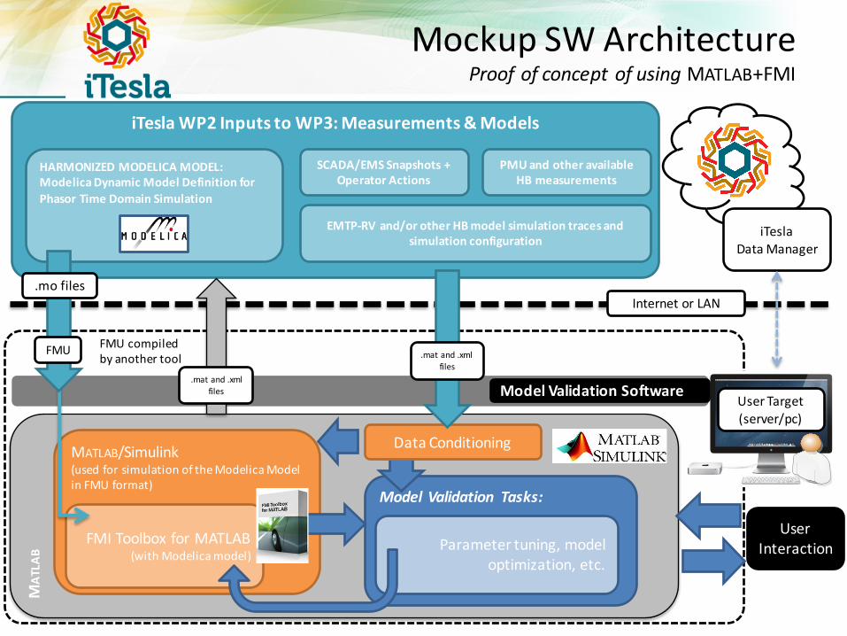
User Target(server/pc)
Model Validation Software
iTesla WP2 Inputs to WP3: Measurements & Models
Mockup SW ArchitectureProof of concept of using MATLAB+FMI
EMTP-‐RV and/or other HB model simulation traces and simulation configuration
PMU and other available HB measurements
SCADA/EMS Snapshots + Operator Actions
MAT
LAB
MATLAB/Simulink (used for simulation of the Modelica Modelin FMU format)
FMI Toolbox for MATLAB(with Modelicamodel)
Model Validation Tasks:
Parameter tuning, model optimization, etc.
User Interaction
.mat and .xml files
HARMONIZED MODELICA MODEL:Modelica Dynamic Model Definition for Phasor Time Domain Simulation
Data Conditioning
iTeslaData Manager
Internet or LAN.mo files
.mat and .xml files
FMU compiled by another tool
FMU

Proof-‐of-‐Concept ImplementationThe RaPId Mock-‐Up Software Implementation
• RaPId is our proof of conceptimplementation (prototype) of a softwaretool for model estimation and validation.The tool provides a framework for modelidentification/validation, mainlyparameter identification.
• RaPId is based on Modelica and FMI –applicable to other systems, not onlypower systems!
• A Modelica model is fed through anFlexibleMock-‐Unit (i.e. FMU) to Simulink.
• The model is simulated and its outputs arecompared againstmeasurements.
• RaPId tunes the parameters of the modelwhile minimizing a fitness criterionbetween the outputs of the simulationand the experimental measurements ofthe same outputs provided by the user.
• RaPId was developed in MATLAB.– The MATLAB code acts as wrapper to
provide interaction with several other programs (which may not need to be coded in MATLAB).
• Advanced users can simply use MATLAB scripts instead of the graphical interface.
• Plug-‐in Architecture:– Completely extensible and open
architecture allows advanced users to add:• Identification methods• Optimization methods• Specific objective functions• Solvers (numerical integration
routines)
Options and
Settings
Algorithm Choice
Results and Plots
Simulink Container
Output measurement data
Input measurement data

What does RaPId do?
Output (and optionally input) measurements are provided to RaPId by the user.
At initialization, a set of parameters is pre-‐configured (or generated randomly by RaPId)The model is simulated with the parameter values given by RaPId.
The outputs of the model are recorded and compared to the user-‐provided measurementsA fitness function is computed to judge how close the measured data and simulated data are to each otherUsing results from (5) a new set of parameters is computed by RaPId.
1
2
3
4
5
2’
ymeas
t
ymeas , ysim
tSimulink ContainerWith Modelica FMU Model
Simulations continue until a min. fitness or max no. of iterations (simulation runs) are reached.
1
2
3
4
5
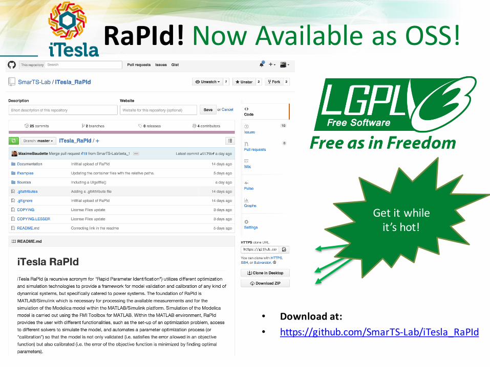
RaPId! Now Available as OSS!
• Download at:• https://github.com/SmarTS-‐Lab/iTesla_RaPId
Get it while it’s hot!

Video Demo!
Validating the Excitation System Model of the Mostar Power Plant!

More On-‐line Video Demos!GUI example
https://www.youtube.com/watch?v=e7OkVEtcz6ACLI example:
https://www.youtube.com/watch?v=4qrPASIWdiY

TAKE AWAYS!Conclussions and Recommendations

Analysis Tools Built with the FMI: xengenModel Freedom = More Flexibility for Analysis
• A view of the future:– What new modelingand simulation technologies can allow users to do
with their models when they are free from a specific tool.– Collaboration with Michael Tiller, Xogeny: http://www.xogeny.com
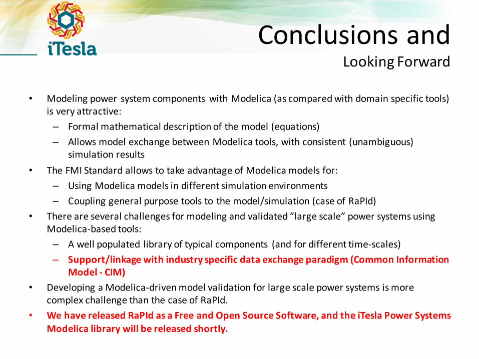
Conclusions andLooking Forward
• Modeling power system components with Modelica (as compared with domain specific tools) is very attractive:– Formal mathematical description of the model (equations)– Allows model exchange between Modelica tools, with consistent (unambiguous)
simulation results• The FMI Standard allows to take advantage of Modelica models for:
– Using Modelica models in different simulation environments– Coupling general purpose tools to the model/simulation (case of RaPId)
• There are several challenges for modeling and validated “large scale” power systems using Modelica-‐based tools:– A well populated library of typical components (and for different time-‐scales)– Support/linkage with industry specific data exchange paradigm (Common Information
Model -‐ CIM)• Developing a Modelica-‐driven model validation for large scale power systems is more
complex challenge than the case of RaPId. • We have released RaPId as a Free and Open Source Software, and the iTesla Power Systems
Modelica library will be released shortly.
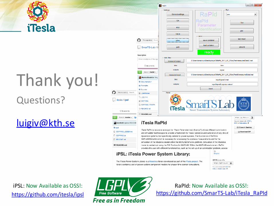
Thank you!Questions?
48
RaPId: Now Available as OSS!: https://github.com/SmarTS-‐Lab/iTesla_RaPId
iPSL: Now Available as OSS!:https://github.com/itesla/ipsl