warehouses on the rise: a study on ceiling height and

1

WAREHOUSES ON THE RISE:

A STUDY ON CEILING HEIGHT AND INVESTMENT VALUE

LESLEY KUIPER

S2200414

OCTOBER 2020

2

COLOFON

Title Warehouses on the rise: a study on ceiling height and investment value

Version Final version

Author L. Kuiper

Student number S2200414

E-mail [email protected]

Supervisor M.N. Daams

Disclaimer: “Master theses are preliminary materials to stimulate discussion and critical comment.

The analysis and conclusions set forth are those of the author and do not indicate concurrence be the

supervisor or research staff.”

3

ABSTRACT

Real estate characteristics required by logistics firms have changed in recent years. One of these

changes is the demand for buildings with higher ceilings. Existing research suggests conflicting

empirical views on how the investment value of logistics buildings is affected by ceiling height. This

study on logistics real estate examines the possible relationship between ceiling height and investment

value. To this end, linear regression analysis is used to analyze transaction prices per square meter and

capitalization rates, both used as measures of investment value. Based on 2000-2019 data for the

Netherlands, relatively higher investment value is, on average, found for logistics real estate with a

ceiling height exceeding 10 meters compared to logistics properties with a ceiling height lower than 10

meters. However, the price premium declined for ceiling heights above 12 meters. This study is the

first to document that there is a positive, non-linear relationship between ceiling height and investment

value.

Key words: logistics real estate, warehouses, ceiling height, investment value

4

Table of contents

1. Introduction ..................................................................................................................................... 5

2. Methods and data ............................................................................................................................. 7

2.1 Methodology .................................................................................................................................. 7

2.2 Data ............................................................................................................................................... 8

2.3 Study Area ................................................................................................................................... 10

3. Results ........................................................................................................................................... 12

3.1 Basic analysis .............................................................................................................................. 12

3.2 Price per square meter models .................................................................................................... 12

3.3 Cap rate models........................................................................................................................... 15

3.4 Logistics hotspots ........................................................................................................................ 17

4. Discussion ..................................................................................................................................... 20

5. Conclusion ..................................................................................................................................... 21

6. References ..................................................................................................................................... 21

7. Appendix ....................................................................................................................................... 23

5

1. Introduction

Logistics real estate1 is one of the largest asset classes of commercial real estate, facilitating a variety

of logistics operations. As a business, logistics has become one of the most important components of

the global economy, linking both production to production and production to consumption (Mattarocci

& Pekdemir, 2017). E-commerce has partly shifted consumption from traditional brick-and-mortar

stores to online shopping. This shift has increased retail vacancy rates, causing demand for retail stores

to drop. Meanwhile online shopping has resulted in a rising demand for logistics properties. However,

there are more factors affecting demand in logistics properties, such as property characteristics

(Treadwell, 1988). More specifically, technological developments over the years have changed

occupiers’ requirements of logistics properties. As a result, ceiling height appears to have become of

increased importance for occupiers and investors nowadays, as brokerage Dynamis (2019) suggests.

The aim of this paper, therefore, is a novel effort to assess scientifically whether the ceiling height of

logistics properties affects investment value.

Whereas a wide range of empirical studies examine the investment value of physical characteristics of

commercial real estate, most focus on offices (Szweizer, 2019); on retail (Newell & Peng Hsu, 2007;

Wiley & Walker, 2011); or on commercial real estate as a whole (Dobson & Goddard, 1992; Bokhari

& Geltner, 2018); but only sometimes on (light) industrial real estate (Lockwood & Rutherford, 1996).

Studies that do incorporate ceiling height specifically, focus on asset price or market rent rather than

investment value (Ambrose, 1990; Buttimer, Rutherford, & Witten, 1997; Fehribach, Rutherford, &

Eakin, 1993; McDonald & Yurova, 2007).

One of the earliest papers on light industrial real estate and ceiling height is done by Ambrose (1990).

His study found no significant relationship between asking price of light industrial properties and

ceiling height, but did find a significant negative relationship between ceiling height and lease rent.

Buttimer et al (1997) tried to examine what characteristics of warehouses influence the market rent.

Their research included, amongst others, the number of high grade doors, ceiling height, percentage of

office space and building age. In accordance with previous studies they found a negative effect of

ceiling height on market rent, which would indicate that occupiers of logistics properties in fact seem

to pay less rent for buildings with higher ceilings. Fehribach et al (1993) performed a similar study as

Ambrose, although including several locational, financial and economic factors. This study did find a

positive significant relationship between ceiling height and asset value. Research by McDonald and

Yurova (2007) on property taxation and selling prices of industrial real estate in the norther Chicago

1 Logistics real estate covers all properties used in the logistics business. The two most common ones are warehouses and

distribution centers. Traditionally, warehouses are used for stockpiling inventory, meaning goods can be stored in warehouses

for months. Modern day supply chains however are better able to predict short term demand, and have therefor shifted their

focus from storing goods to transhipment, requiring multiple loading docks. These buildings are known as distribution

centers. In order to qualify as a distribution center the floor space has to exceed 5,000 square meters, whilst also having one

loading dock per 1,000 square meters of floor space. In this research both warehouses and distribution centers are included.

6

region included data on ceiling height and several other property characteristics. They found a

positive, but insignificant relationship between ceiling height and selling price.

It is clear that previous research does not agree on the effect ceiling height has on property value.

However, it is important to consider the fact that the previously mentioned studies are outdated. The

average ceiling height in these studies’ dataset ranges from approximately 4.5 meters to 6.0 meters. In

comparison, in 2009 newly built distribution centers required a clear height2 of 10.8 meters (DTZ,

2009). More recently the requirements have risen to 12.2 meters (Dynamis, 2018). From these changes

in requirements one can conclude that older logistics properties are suffering from functional

obsolescence (‘economic aging’), which should have a negative impact on their investment value

(Mansfield & Pinder, 2008).

However, in most of the previously mentioned studies the occupiers of logistics properties are the

subject, since the focus is either on market rent or on selling price from an owner-occupier’s

perspective. Owner-occupiers often have different views on how to value real estate compared to

investors. Owner-occupiers plan on utilizing the property themselves. They seek for property

characteristics that fit their specific business, which could lead to overvaluation of certain

characteristics in order to fit their needs. Investors seek for property characteristics that fit a variety of

businesses, since it would be easier to find a new lessee when the lease contract expires. The

investor’s view would therefore give a more representative picture of what property characteristics are

valued by the logistics market overall. Therefore, this paper’s contribution is to examine the

relationship between ceiling height and investment value from an investor’s perspective.

The aim of this study is to examine the possible relationship between ceiling height and investment

value of logistics real estate. Data on logistics real estate investment transactions are used (N = 1,200)

All of these transactions include transaction prices, while some of the include capitalization rates as

well. The capitalization rate, or cap rate, is the net operating income divided by the price paid. For real

estate that means the net annual rent income from a property, divided by the transaction price of that

same property. A high cap rate indicates that the net annual rent is relatively large compared to the

transaction price. This means the payback time for the investment could be shorter. However, higher

cap rates indicate that investors perceive the investment’s risk to be higher as well. Transactions with

lower cap rates reflect that these properties have a higher investment value, as investors perceive them

as less risky investments. Using both transaction prices and cap rates gives an insight in not only how

ceiling height affects prices, but also how it affects the perceived risk for investors, which is

2 Clear height is defined as the height of a building from the floor to the lowest hanging item on the ceiling. This concerns the

maximum height which can be used to stockpile inventory. The difference between clear height and ceiling height is 1,5

meters on average.

7

incorporated in cap rates. The dataset on transactions are combined with information from an elevation

map, which includes building height for all buildings in the Netherlands.

2. Methods and data

2.1 Methodology

This study tests whether the investment value of logistics properties is affected by its ceiling height.

To do so, this study uses linear regression models to describe the relationship between the various

dependent and independent variables. This method uses several explanatory variables to explain the

variance in a dependent variable. Additionally, this method allows for continuous variables as well as

categorical variables to be included, which fits the used dataset. The analysis shows in what way and

how much the dependent variable is affected by the independent variables, in this case indicating how

investment value is affect by, amongst others, ceiling height.

The dependent variables are either price per square meter or cap rate, and the variable of interest is the

independent variable ceiling height. The first part of the analysis concerns the dependent variable price

per square meter. The specification of the first model (1) for property i (i=1,…,n) at time t is

ln𝑃𝑖𝑡 = 𝛼 + ln𝛽1𝐶𝑖𝑡 + ln𝛽2𝐹𝑖𝑡 + 𝛽3𝐴𝑖𝑡 + 𝛽𝑋𝑋𝑖 + 𝜀𝑖𝑡 (1)

where α is the constant; lnPit is the natural log of the transaction price per square meter; lnβ1Cit is the

natural log of ceiling height; lnβ2Fit is the natural log of floor space; β3Ait is a dummy for building

period; βxXi are control variables for location and time fixed effects; and εit is the error term. The log-

log functional model is used because the continuous variables price per square meter, ceiling height

and floor space all have a right-side tail, (see Appendix A). A dummy for a specific building period is

used for the building age. In this case five building periods are chosen, based on the development of

the logistics real estate market throughout the years (Aquila Capital, 2020). Development of the

logistics market changes requirements of newly built properties. Therefore periods are chosen for

older buildings (pre-1980), first logistics developments (1980-1999), increased growth up to the

financial crisis (2000-2007), aftermath of the crisis (2008-2013), and recent rapid developments

(2014-2019). Control variables are added to control for location by zip code and transaction year.

The following models try to examine whether there is a minimum or maximum ceiling height for

which a premium is paid, using a dummy variable for ceiling height rather than a continuous variable.

The specification of the next models (2-5) for property i (i=1,…,n) at time t is

ln𝑃𝑖𝑡 = 𝛼 + 𝛽1𝐶𝑑𝑖𝑡 + ln𝛽2𝐹𝑖𝑡 + 𝛽3𝐴𝑖𝑡 + 𝛽𝑋𝑋𝑖 + 𝜀𝑖𝑡 (2-5)

where, besides the independent variable for ceiling height, the same variables are used as in model (1).

In this model ceiling height is determined by dummy variable β1Cdit, indicating whether the ceiling

8

height is higher or lower than the specified height. This includes dummies for ceiling heights higher

than 10 meters, 11 meters, 12 meters, and 13 meters.

Similar model specifications are used for the second part of the analysis, using cap rate as de

dependent variable. The specification for models (6) and (7) for property i (i=1,…,n) at time t is

ln𝑌𝑖𝑡 = 𝛼 + ln𝛽1𝐶𝑖𝑡 + ln𝛽2𝐹𝑖𝑡 + 𝛽3𝐴𝑖𝑡 + 𝛽𝑋𝑋𝑖 + 𝜀𝑖𝑡 (6-7)

where dependent variable lnYit is the natural log of cap rate. The independent variables are identical to

the independent variables used in model (1). However, for the analyses on cap rates the sample size is

smaller than for the analyses on price per square meter, hence some adaptations are done. Year

dummies are omitted, and instead of five building periods to control for building age, only three

periods are used. Building age is a known determinant for cap rates. In order to examine the effect this

variable has on cap rates, in model (7) there are no variables used for building period.

Finally, the next models again specify ceiling height as a dummy variable, in order to find a possible

minimum or maximum ceiling height for a cap rate premium. The specifications for models (8-11) for

property i (i=1,…,n) at time t is

ln𝑌𝑖𝑡 = 𝛼 + 𝛽1𝐶𝑑𝑖𝑡 + ln𝛽2𝐹𝑖𝑡 + 𝛽3𝐴𝑖𝑡 + 𝛽𝑋𝑋𝑖 + 𝜀𝑖𝑡 (8-11)

where β1Cdit is a dummy variable to determine ceiling height, as in models (2-5). The other variables

are similar to models (6-7).

As mentioned before, the increased average ceiling height requirements by logistics buildings users

appears to have risen in recent years. This could indicate that investors find logistics properties with

higher ceilings more valuable than logistics properties with lower ceilings. Therefore it is expected

that there is a positive relationship between ceiling height and price per square meter, which would be

in line with Fehribach et al. (1993). Similar principles apply for the models using cap rate as the

dependent variable. Although, the coefficient for ceiling height is expected to be negative, since lower

cap rates are an indicators for higher investment value.

2.2 Data

The Strabo data consists of 1,663 logistics real estate investment transactions from 2000-2019, across

all regions in the Netherlands. The observations cover all known transactions which are categorized as

logistics properties, both current buildings as well as newly built properties. The dataset includes

information on transaction price, zip code, sales price, floor space, and in 149 cases cap rates.

9

Data on ceiling height is not included in the dataset provided. Since data on clear height is not freely

available, this study uses ceiling height as an estimate of clear height. In order to estimate the clear

height of the observed buildings, a height map of the Netherlands is used, provided by the Actueel

Hoogtebestand Nederland (AHN). This height map consists of a grid, including ground height as well

as roof height for each grid. The 3D Geoinformation Group (2019)3 created the 3D BAG, in which

AHN data on height is combined with the BAG (Basisadministratie Adressen en Gebouwen)

(Kadaster, 2019). Merging this data with the original dataset provides height data for each building.

Subtracting the ground height from the roof height indicates the height of a specific building. Since

logistics properties have large floorspace, most buildings cover multiple grids of the height map. This

often results in multiple, sometimes varying, observations of roof height. However, in most cases the

variations are minimal. In case a property has multiple roof levels the highest roof is used as a

reference. In this study the roof height is used as an estimate for ceiling height. Additionally, from the

BAG, information is added on the year in which the warehouse or distribution center is built.

After cleaning, the final dataset consists of 1,200 observations, including the variables sales price,

ceiling height, floor space, and building age4. In order to show a better comparison between

warehouses, this research uses the sales price per square meter as the dependent variable rather than

the absolute sales price. Additionally, of 117 observations the cap rate is known. Dummy variables are

used to control for location, based on zip codes5, and for transaction year. Descriptive statistics for the

estimation sample are provided in Table 1. The average ceiling height in the dataset is 10.86 meters

3 The 3D geoinformation research group is part of the Department of Urbanism, Faculty of Architecture and the Built

Environment of the Delft University of Technology. 4 Multiple cases of missing data were observed after merging the main dataset with AHN and BAG data, meaning several

logistics transactions could not be matched in the height map. After reviewing these missing observations it can be concluded

that however logistics transactions are provided up to late 2019, the newly built logistics properties are not yet included in the

AHN dataset and can therefore not be used. Additionally, several properties in the transaction data have been demolished and

their original building height can therefore not be traced back, and some transactions concern portfolio sales, which cover

more than one warehouse, or a combination of warehouses and offices. Since building height is an essential variable of this

research, all observations which could not be matched are dropped. This concerns a total of 387 observations. In case of

missing observations concerning floor space the BAG has been accessed and floor space has been added manually. The floor

space of 66 observations could not be retrieved and are therefore dropped since they are considered unrealistic. Moreover,

observations with a sales price that exceeds EUR 3,000 per square meter are dropped. This concerns another 6 observations.

These sales included value-added factors which makes them less representative. 5 Location by zip code is defined as PC1000 up to PC9000 for nine zip code areas in the Netherlands, where PC1000 includes

all zip codes from 1000 to 1999, PC2000 includes zip codes from 2000 to 2999, up to PC9000. Zip codes are used because

they best reflect the logistics regions in the Netherlands.

Table 1 - Descriptives

Variable Average Std. Dev. N

Price (EUR/m²) 655.72 341.61 1,200

Cap rate 0.081 0.015 117

Ceiling height (m) 10.86 3.26 1,200

Floor space (m²) 17,481.25 17,812.77 1,200

Building age (years) 28.37 17.04 1,200

10

(st.dev. = 3.26), which is remarkably higher than the average ceiling height in the previously

mentioned studies. Moreover, the independent variables floor space and building age have high

standard deviations, indicating that there is a large range of observations in terms of building size and

age.

2.3 Study Area

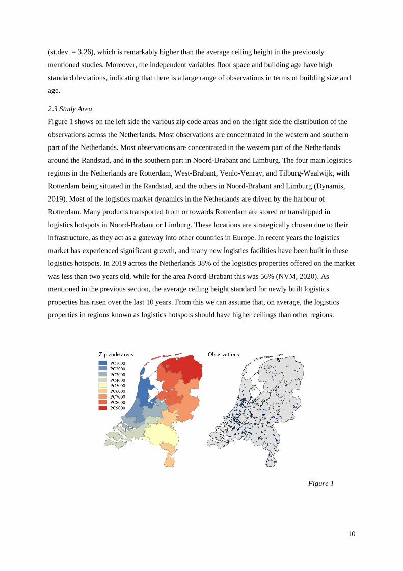
Figure 1 shows on the left side the various zip code areas and on the right side the distribution of the

observations across the Netherlands. Most observations are concentrated in the western and southern

part of the Netherlands. Most observations are concentrated in the western part of the Netherlands

around the Randstad, and in the southern part in Noord-Brabant and Limburg. The four main logistics

regions in the Netherlands are Rotterdam, West-Brabant, Venlo-Venray, and Tilburg-Waalwijk, with

Rotterdam being situated in the Randstad, and the others in Noord-Brabant and Limburg (Dynamis,

2019). Most of the logistics market dynamics in the Netherlands are driven by the harbour of

Rotterdam. Many products transported from or towards Rotterdam are stored or transhipped in

logistics hotspots in Noord-Brabant or Limburg. These locations are strategically chosen due to their

infrastructure, as they act as a gateway into other countries in Europe. In recent years the logistics

market has experienced significant growth, and many new logistics facilities have been built in these

logistics hotspots. In 2019 across the Netherlands 38% of the logistics properties offered on the market

was less than two years old, while for the area Noord-Brabant this was 56% (NVM, 2020). As

mentioned in the previous section, the average ceiling height standard for newly built logistics

properties has risen over the last 10 years. From this we can assume that, on average, the logistics

properties in regions known as logistics hotspots should have higher ceilings than other regions.

Figure 1

11

Figure 2 shows from left to right the average price per square meter, average cap rate, and average

ceiling height for every zip code area. The highest average price per square meter is paid in the zip

code area PC1000. This could be explained by the fact that airport Schiphol is situated in this area.

Large airports transfer a lot of freight with results in high demand for local warehouses. Other zip code

areas in which a high average price per square meter is paid are PC2000, which is close to airport

Schiphol as well, and PC5000. This area, covering the eastern part of Noord-Brabant and the northern

part of Limburg, is known as a logistics hotspot, as mentioned before.

The lowest cap rates are found in zip code area PC4000. This area borders the Randstad, in which the

four biggest cities of the Netherlands are situated. The zip code area with the second lowest average

cap rates is area PC5000. The number of observations in cap rate are scarce, and do not cover the

entire country. No cap rates are observed in zip code area PC9000, in the north of the Netherlands.

Zip code area PC5000 has the highest average ceiling height, followed by PC6000, PC2000, and

PC1000. Taking into account the high average price per square meter in the area around the Randstad

in zip code areas PC1000 and PC2000 and the lowest average cap rate in zip code area PC5000, it

could be possible that there is a relationship between both dependent variables price per square meter

and cap rate, and the main independent variable ceiling height. An explanation could be that higher

ceilings provide more volume, and therefore more options for a variety of firms to conduct their

business. From an investor’s perspective this would be interesting, since vacant space is absorbed

quicker, reducing overall risk of the investment. In order to control for regional differences dummy

variables are used.

Figure 2

12

3. Results

3.1 Basic analysis

In order to analyze whether there are relationships between the dependent variables price per square

meter and cap rate on the one hand and independent variable ceiling height on the other hand, two

scatterplots are made. Graph 1 and Graph 2 show these scatterplots. Graph 1 shows the price per

square meter on the y-axis and the ceiling height on the x-axis. Interesting is the upward sloping

regression line6, indicating that there is a positive relationship between price per square meter and

ceiling height. Graph 2 shows the regression line7 with cap rate on the y-axis and ceiling height on the

x-axis. The fitted line shows a negative relationship between cap rate and ceiling height. This provides

an important initial confirmation of this study’s expectation that increased ceiling height results in a

higher price per square meter and results in a lower cap rate, both indicating increased investment

value.

To assess these relationships in more detail, by controlling the characteristics of buildings, their

locations, and transaction dates, we now turn to the results for the regression models.

3.2 Price per square meter models

Table 2 shows the regression results of the models (1-5), with the natural log of price per square meter

as dependent variable. Besides the independent variable ceiling height, the other independent variables

show similar coefficients across all five models. There is a significant negative relationship between

log floor space and log price per square meter. This is an expected finding, since usually increased

6 The regression line is Price per square meter = 11.3689 [3.0176] * Ceiling height + 532.1782 [34.2272]

with R2 = 0.0117 and N = 1,200 7 The regression line is Cap rate = -0.0008 [0.0004] * Ceiling height + 0.0901 [0.0052]

with R2 = 0.0291 and N = 117

Graph 1 Graph 2

13

floor space results in a declining price per square meter. The variables concerning building periods

later than the year 2000 are all highly significant, while the variable building period 1980-1999 is not.

This indicates that there is a significant difference in price per square meter between logistics

buildings constructed before the year 2000, and the ones constructed after the year 2000. Moreover,

the R2 appears to be rather constant across all five models.

Now we turn to the variable of interest, ceiling height. The five models shown, use different

independent variables in term of clear height. The other independent variables are similar. The first

model (1) uses the natural log of ceiling height as the determinant for ceiling height. The coefficient of

0.156 is highly significant, indicating that for every 1% increase in ceiling height, the price per square

meter increases by 0.156%. The models for various ceiling heights (2-5) show that ceiling height

higher than 10 meter, 11 meter, 12 meter and 13 meters, on average, increase value. Noteworthy is that

the coefficient for the dummy variable ceiling height higher than 11 meters is the highest compared to

the other models. This coefficient of 0.131 indicates that properties with a ceiling height higher than

11 meters, on average, have a 14% higher price per square meter than properties with a ceiling height

lower than 11 meters. For properties with a ceiling height higher than 10 meters the price per square

meter is 9% higher, for properties higher than 12 meters this is 12% and for properties higher than 13

meters this is 8%. This indicates that for the used sample there is a non-linear relationship between

ceiling height and price per square meter. These results suggest that the relative premium paid for

building with a ceiling height higher than 12 and 13 meters declines compared to buildings with a

ceiling height higher than 11 meters.

14

Table 2 - Linear regression results equation 1: dependent variable log price per m²

(1) (2) (3) (4) (5)

Log ceiling height 0.156

(0.054)***

Ceiling height 10 m +

0.090

(0.032)***


0.131

(0.032)***


0.112

(0.033)***


0.081

(0.035)**

Log floor space -0.115 -0.113 -0.120 -0.116 -0.105

(0.017)*** (0.017)*** (0.017)*** (0.017)*** (0.016)***

Building period 1980-1999 0.022 0.025 0.020 0.026 0.035

(0.037) (0.037) (0.037) (0.037) (0.037)

Building period 2000-2007 0.190 0.190 0.174 0.187 0.211

(0.045)*** (0.045)*** (0.045)*** (0.045)*** (0.044)***

Building period 2008-2013 0.439 0.442 0.420 0.429 0.454

(0.056)*** (0.056)*** (0.056)*** (0.056)*** (0.055)***

Building period 2014-2019 0.444 0.450 0.428 0.435 0.443

(0.068)*** (0.068)*** (0.068)*** (0.069)*** (0.069)***

Zip code PC1000 0.079 0.077 0.077 0.090 0.085

(0.110) (0.110) (0.110) (0.110) (0.110)

Zip code PC2000 0.017 0.025 0.019 0.024 0.022

(0.112) (0.112) (0.112) (0.112) (0.113)

Zip code PC3000 -0.032 -0.034 -0.037 -0.030 -0.034

(0.109) (0.109) (0.109) (0.109) (0.109)

Zip code PC4000 -0.016 -0.021 -0.030 -0.020 -0.014

(0.111) (0.115) (0.111) (0.111) (0.111)

Zip code PC5000 -0.020 -0.022 -0.028 -0.015 -0.016

(0.110) (0.111) (0.110) (0.110) (0.111)

Zip code PC6000 -0.135 -0.138 -0.148 -0.134 -0.133

(0.115) (0.115) (0.114) (0.114) (0.115)

Zip code PC7000 -0.298 -0.308 -0.314 -0.294 -0.294

(0.120)** (0.120)** (0.120)*** (0.120)** (0.120)**

Zip code PC8000 -0.168 -0.168 -0.182 -0.158 -0.158

(0.134) (0.134) (0.139) (0.134) (0.134)

Constant 6.149 6.469 6.541 6.482 6.361

(0.393)*** (0.395)*** (0.393)*** (0.394)*** (0.341)***

Adj. R² 0.300 0.299 0.305 0.302 0.298

N 1,200 1,200 1,200 1,200 1,200

Notes: Year dummies not shown

Reference category building period = building period pre-1980

Reference category zip code = PC9000

*p < 0.10; **p < 0.05; ***p < 0.01.

15

3.3 Cap rate models

Model (6) uses the natural log of ceiling height as the determinant for ceiling height. A weakly

significant negative relationship is found. A 1% increase in ceiling height results in a 0.096% decrease

in cap rate at a 10% significance level. Since the coefficient of building period 2014-2019 is highly

significant, it could be that the effect of height is diminished due to this dummy. Model (7) omitted the

dummies for building periods. It shows that the coefficient of log ceiling height is larger than in model

(6), indicating that these dummies do have a significant effect on log cap rate. However, this has a

negative effect on the model fit, since the adjusted R2 is only 0.156 compared to 0.198 in model (6).

Models (8-11) include dummy variables to determine ceiling height, ranging from 10 meters and

higher to 13 meters and higher. The only model where a significant coefficient for ceiling height is

found is model (9). The coefficient of -0.061 indicates that logistics properties with a ceiling height

higher than 11 meters, tend to have a cap rate which is, on average, 6.1% lower than properties with a

ceiling height lower than 11 meters. The effect, however, is weakly significant. Nevertheless, we can

see from the standard errors for the other models that while the ceiling height coefficients in those

models are insignificant, the estimates are quite close to being significant at the level as in model (9).

It is important to keep in mind that properties are heterogenous. Cap rates are influenced by a variety

of characteristics, with ceiling height being one of them. This, combined with the small sample size,

could explain to the weakly significant results. However, when considering the previous models on

price per square meter, a consistent effect seems apparent for buildings with a ceiling height exceeding

10 meters.

16

Table 3 - Linear regression results - dependent variable log cap rate

(6) (7) (8) (9) (10) (11)

Log ceiling height -0.096 -.111

(0.058)* (0.057)*

Ceiling height 10+ m

-0.059

(0.036)


-0.061

(0.033)*


-0.042

(0.033)


0.010

(0.034)

Log floor space 0.010 0.010 0.014 0.013 0.009 -0.000

(0.022) (0.022) (0.022) (0.022) (0.022) (0.021)

Building period 2008-2013 0.015

0.012 0.014 0.006 -0.006

(0.048)

(0.048) (0.048) (0.048) (0.049)

Building period 2014-2019 -0.159

-0.168 -0.162 -0.163 -0.179

(0.060)***

(0.059)*** (0.059)*** (0.060)*** (0.061)***

PC1000 -0.104 -0.092 -0.098 -0.107 -0.110 -0.120

(0.066) (0.067) (0.066) (0.065) (0.066) (0.066)

PC2000 -0.052 -0.035 -0.053 -0.048 -0.052 -0.066

(0.064) (0.066) (0.064) (0.064) (0.065) (0.065)

PC3000 0.079 0.091 0.081 0.079 0.076 0.066

(0.061) (0.062) (0.061) (0.060) (0.061) (0.061)

PC4000 -0.148 -0.153 -0.140 -0.140 -0.140 -0.145

(0.060)** (0.061)** (0.060)** (0.060)** (0.060) (0.061)**

PC5000 -0.097 -0.109 -0.095 -0.096 -0.098 -0.107

(0.053)* (0.054)** (0.053)* (0.053)* (0.054)* (0.054)**

PC6000 -0.121 -0.103 -0.118 -0.119 -0.123 -0.134

(0.071)* (0.072) (0.072) (0.071) (0.072)* (0.072)*

Constant -2.318 -2.295 -2.552 -2.549 -2.522 -2.448

(0.226)*** (0.230)*** (0.219)*** (0.217)*** (0.218)*** (0.214)***

Adj. R² 0.198 0.156 0.197 0.202 0.190 0.178

N 117 117 117 117 117 117

Notes: Reference category building period = building period pre-2008

Reference category zip code = PC7000, PC8000, PC9000

*p < 0.10; **p < 0.05; ***p < 0.01.

17

3.4 Logistics hotspots

After reviewing the results of both dependent variables price per square meter and cap rate it is

interesting to look more in-depth into regional logistics hotspots. In a previous section the various

logistics hotspots in the Netherlands were mentioned, as well as the fact that significant regional

differences exist in the Dutch logistics market. Some regions have a higher percentage of newly built

properties than others, which could indicate that the effect of ceiling height on investment value is

different in these regions relative to the country as a whole. In order to examine this a more in-depth

analysis is performed for regions known as logistics hotspots.

Firstly we look at the distribution of observations across the nine zip code areas in The Netherlands,

which is shown in Graphs 3 and 4.

Graph 3 shows that the number of price per square meter observations for most zip code areas should

be sufficient for performing analyses. However, Graph 4 shows that the number of cap rate

observations for each zip code area is rather low. However, PC5000 stands out, with 35 observations.

The area PC5000 includes the largest part of Noord-Brabant and the northern part of Limburg, and is

known as a logistics hotspot. Figure 2 in section 3.3 showed that this region has notable patterns, with

high average ceiling height, high average price per square meter, and low average cap rate. Moreover,

in 2019 the region Tilburg-Waalwijk and the region Venlo-Venray were chosen as the numbers one

and two logistics hotspots in the Netherlands by a panel of logistics experts (Logistiek.nl, 2019). The

experts took into account, amongst others, the access to qualified personnel, local government

involvement, and physical accessibility. The in-depth analysis will focus on the area with zip code

PC5000, since it is apparent that the largest logistics hotspots are located in this area.

Graph 3 Graph 4

18

Table 4 - Linear regression zip code area PC5000: dependent variable log price per m2

(12) (13) (14) (15) (16)

Log ceiling height 0.208

(0.119)*


0.020

(0.076)


0.149

(0.071)**


0.133

(0.068)*


0.092

(0.068)

Log floor space -0.107 -0.089 -0.111 -0.110 -0.098

(0.036)*** (0.036)** (0.036)*** (0.036)*** (0.035)***

Building period 1980-1999 0.130 0.143 0.118 0.137 0.144

(0.101) (0.102) (0.101) (0.101) (0.101)

Building period 2000-2007 0.133 0.162 0.108 0.134 0.148

(0.100) (0.100) (0.101) (0.099) (0.099)

Building period 2008-2013 0.386 0.428 0.367 0.370 0.397

(0.109)*** (0.108)*** (0.110)*** (0.110)*** (0.110)***

Building period 2014-2019 0.534 0.550 0.508 0.515 0.516

(0.129)*** (0.130)*** (0.130)*** (0.130)*** (0.131)***

Constant 6.162 6.461 6.612 6.587 6.488

(0.579)*** (0.566)*** (0.560)*** (0.560)*** (0.559)***

Adj. R² 0.148 0.135 0.154 0.152 0.143

N 214 214 214 214 214

Notes: Year dummies not shown

Reference category building period = building period pre-1980

*p < 0.10; **p < 0.05; ***p < 0.01.

The models used for this analysis are roughly the same models which are used for the total sample.

Firstly, table 4 shows models (12-16) with regression results for zip code area PC5000, using the

natural log per square meter as the dependent variable. The coefficient for log ceiling height is higher

than the same coefficient for the total sample, indicating ceiling height has more influence on the price

per square meter in this area compared to the national average. Furthermore, the coefficient of the

dummy ceiling height higher than 11 meters is larger than the dummy of ceiling height higher than 12

meters. This is conform the findings of the total sample models, which indicates that the effect of

ceiling height on price per square meter is non-linear and the premium paid decays when height

exceeds 12 meters.

19

Secondly, the regional differences are tested using the natural log of cap rate as the dependent

variable. Due to the relatively few observations in the area PC5000 the previously used model has to

be adjusted accordingly. Year dummies have not been used in this model, and only three time periods

have been used indicating building age. The results are shown in Table 5.

Table 5 - Linear regression zip code area PC5000 - dependent variable log cap rate

(17) (18) (19) (20) (21)

Log ceiling height -0.240

(0.094)**


-0.100

(0.057)*


-0.094

(0.052)*


-0.074

(0.053)


-0.028

(0.053)

Log floor space 0.032 0.029 0.029 0.027 0.013

(0.029) (0.031) (0.031) (0.032) (0.031)

Building period 2008-2013 0.040 0.010 0.022 0.024 0.005

(0.065) (0.066) (0.067) (0.069) (0.069)

Building period 2014-2019 -0.119 -0.153 -0.142 -0.140 -0.146

(0.060)* (0.061)** (0.062)** (0.064)** (0.070)**

Constant -2.287 -2.768 -2.789 -2.786 -2.680

(0.317)*** (0.299)*** (0.300)*** (0.310)*** (0.307)***

Adj. R² 0.238 0.159 0.164 0.130 0.082

N 35 35 35 35 35

Notes: Reference category building period

= building period pre-2008

*p < 0.10; **p < 0.05; ***p < 0.01.

The coefficient of log ceiling height is more than twice as large as the coefficient of log ceiling height

for the model covering the total sample. Moreover, interesting is the difference between the

coefficients of ceiling height higher than 10 meters and ceiling height higher than 11 meters, which are

negative 0.100 and negative 0.094, respectively. As opposed to the total sample, in this area there

seems to be a significant effect of ceiling height on cap rate from 10 meters and higher, while in the

total sample only a significant effect is found for a ceiling height higher than 11 meters. Furthermore,

the effect seems to decline, which is in line with the results of the previous models.

20

4. Discussion

While the effect of property characteristics on commercial real estate has been investigated before, this

research is the first to extensively study the effect of ceiling height on the investment value of logistics

real estate. The investment volume of logistics properties has been increasing every year, and this

study aimed to find a better understanding on how investment value is affected at the micro-level.

The results from the performed analyses are in line with the expectations, namely that ceiling height

has a positive relationship with investment value. A positive effect is found of ceiling height on price

per square meter, while a negative effect is found of ceiling height on cap rate. This is in line with

Fehribach et al. (1993), who as well found a significant positive relationship between ceiling height

and asset value. Moreover, this study finds that the premium effect of ceiling height on investment

value flattens when the ceiling height exceeds 12 meters, which implies that the effect is non-linear. At

first hand the non-linear relationship seems abnormal. Logically, one could assume that higher ceilings

offer more storage volume, thus increasing the price. Logistics properties however have to follow

specific safety measures, and one of these measures is fire safety using a sprinkler installation. Usually

sprinklers are attached to the lowest hanging structure on the ceiling, which is the clear height, at a

maximum height of 12.2 meters (FM Global, 2010). In case the clear height exceeds this maximum

height either the sprinklers must be attached to the stockpiled inventory or machines, or more

expensive sprinklers must be installed to the roof structure. According to R. Kroon, of the department

Capital Transactions at Goodman, most logistics developers however claim that the increased benefit

of efficiency due to a higher ceiling does not outweigh the cost of the more expensive sprinkler

installation (Kroon, 2020).

This study used ceiling height, floor space, and building age as determinants for property

characteristics of logistics real estate. However, previous research has shown that for example number

of truck or high grade doors, and floor capacity are important determinants as well (Ambrose, 1990;

Treadwell, 1988). The limited availability of data concerning property characteristics results from a

lack of transparency in the commercial real estate market as a whole, since many transactions are not

publicized by brokerages. The total number of transactions therefore is higher than the number of

transactions used in this research. Moreover, often times when transactions are publicized, specific

determinants for property characteristics are not included. Although there is a lack of transparency in

the commercial real estate market, incorporating these determinants in future research that uses more

comprehensive data, which are only scarcely available to academic researchers in the field of real

estate economics, would be a meaningful addition to academic literature.

21

5. Conclusion

The aim of this research was to determine a relationship between logistics properties’ ceiling height

and their investment value. Strabo data was used in a linear regression model to determine how ceiling

height affects both price per square meter and cap rate, which are determinants for investment value.

Crucially, a reasonably significant positive relationship was found between ceiling height and price

per square meter. Additional models suggest that the relationship between ceiling height and price per

square meter is non-linear. That is, the premium paid for a logistics property is found to decline when

the ceiling height surpasses 12 meters. When considering cap rates, a similar pattern is found, as

flattening of the positive price-effect sets in for properties with a ceiling height higher than 12 meters

as well. Furthermore, when considering a specifically dynamic logistics region, the findings even more

clearly show an effect of ceiling height on investment value.

6. References

Ambrose, B. W. (1990). An Analysis of the Factors Affecting Light Industrial Property Valuation. The

Journal of Real Estate Research, 5(3), 355-370.

Bokhari, S., & Geltner, D. (2018). Characteristics of Depreciation in Commercial and Multifamily

Property: An Investment Perspective. Real Estate Economics, 46(4), 745-782.

Buttimer, R. J., Rutherford, R. C., & Witten, R. (1997). Industrial Warehouse Rent Determinants in

the Dallas/Fort Worth Area. The Journal of Real Estate Research, 13(1), 47-55.

Dobson, S. M., & Goddard, J. A. (1992). The determinants of commercial property prices and rents.

Bulletin of Economic Research, 44(4), 301-321.

DTZ. (2009). Logistiek is rekenkunst.

Dynamis. (2018). Sprekende cijfers: marktscan logistiek. Dynamis B.V.

Dynamis. (2019). Sprekende Cijfers Logistiek 2019. Utrecht.

Fehribach, F. A., Rutherford, R. C., & Eakin, M. E. (1993). An analysis of the determinants of

industrial property valuation. The Journal of Real Estate Research, 8(3), 365-376.

FM Global. (2010). Property Loss Prevention Data Sheets.

Franklin, H. (1994). Industrial Inspirations. Journal of Property Management, 59(3), 18-20.

Hughes, W. T. (1994). Determinants of Demand of Industrial Property. The Appraisal Journal, 62(2),

303-309.

22

Kadaster. (2019). Basisregistratie Adressen en Gebouwen (BAG). Opgeroepen op 12 19, 2019, van

https://bagviewer.kadaster.nl/

Kroon, R. (2020, July 6). personal communication by email. (L. Kuiper, Interviewer)

Lockwood, L. J., & Rutherford, R. C. (1996). Determinants of Industrial Property Value. Real Estate

Economics, 24(2), 257-272.

Logistiek.nl. (2019). Logistieke hotspots van Nederland. Opgehaald van www.logistiek.nl.

Mansfield, J. R., & Pinder, J. A. (2008). "Economic" and "functional" obsolescence: Their

characteristics and impacts on valuation practice. Property Management, 26(3), 191-206.

Mattarocci, G., & Pekdemir, D. (2017). Logistic Real Estate Investment and REIT's in Europe. Cham:

Palgrave Macmillan.

McDonald, J. F., & Yurova, Y. (2007). Property taxation and selling prices of industrial real estate.

Review of Accounting and Finance, 6(3), 273-284.

Myers, J. (1994). Fundamentals of Production That Influence Industrial Facility Designs. The

Appraisal Journal, 62(2), 296-302.

Newell, G., & Peng Hsu, W. (2007). The significance and performance of retail property in Australia.

Journal of Property Investment & Finance, 25(2), 147-165.

NVM. (2020). Logistiek vastgoed in cijfers. Zeist: NVM Business.

Szweizer, M. (2019). A new model for Auckland commercial property yields. Journal of Property

Investment & Finance, 37(1), 42-57.

Treadwell, D. H. (1988). Intricacies of the Cost Approach in the Appraisal of Major Industrial

Properties. The Appraisal Journal(1), 70-79.

Wiley, J. A., & Walker, D. M. (2011). Casino Revenues and Retail Property Values: The Detroit Case.

Journal of Real Estate Finance and Economics, 42, 99-114.

23

7. Appendix

warehouses on the rise: a study on ceiling height and

Documents