Was Stalin Necessary for Russia�s Economic Development?�

Anton Cheremukhin, Mikhail Golosov, Sergei Guriev, Aleh Tsyvinski

April 2013

Abstract

This paper studies structural transformation of Soviet Russia in 1928-1940 from an agrarianto an industrial economy through the lens of a two-sector neoclassical growth model. We con-struct a large dataset that covers Soviet Russia during 1928-1940 and Tsarist Russia during1885-1913. We use a two-sector growth model to compute sectoral TFPs as well as distortionsand wedges in the capital, labor and product markets during the two periods. We �nd thatmost wedges substantially increased in 1928-1935 and then fell in 1936-1940 relative to their1885-1913 levels, while TFP remained generally below pre-WWI trends. Under the neoclassicalgrowth model, projections under these estimated wedges imply that Stalin�s economic policiesled to welfare loss of -24 percent of consumption in 1928-1940, but a +16 percent welfaregain after 1941. A representative consumer born at the start of the Stalin�s policies in 1928experiences a reduction in welfare of -1 percent of consumption, a number that does not takeinto account additional costs of political repression during this time period. The projectedperformance under both Tsarist�and Stalin�s wedges is much worse than the economic per-formance of Japan, which in 1885-1913 had similar levels of per capita GDP and distortionsas Tsarist Russia, but experienced a rapid acceleration of non-agricultural TFP during theinterwar period. Relative to this benchmark, the welfare loss of Stalin�s policies are about -31percent of consumption.

�Cheremukhin: Federal Reserve Bank of Dallas; Golosov: Princeton and NES; Guriev: NES; Tsyvinski: Yaleand NES. The authors thank Mark Aguiar, Bob Allen, Paco Buera, V.V. Chari, Hal Cole, Andrei Markevich, JoelMokyr, Lee Ohanian, Richard Rogerson for useful comments. We also thank participants at the EIEF, FederalReserve Bank of Philadelphia, NBER EFJK, New Economic School, Northwestern, Ohio State, Princeton.Financial support from NSF is gratefully acknowledged. Golosov and Tsyvinski also thank Einaudi Institute ofEconomics and Finance for hospitality. Any opinions, �ndings, and conclusions or recommendations expressedin this publication are those of the authors and do not necessarily re�ect the views of their colleagues, theFederal Reserve Bank of Dallas or the Federal Reserve System.

1 Introduction

In 1962, prominent British economic historian, Alec Nove, posed the question of whether

Russia would have been able to industrialize during of late 1920s and 1930s in the absence of

Stalin�s economic policies.1 The transformation of Soviet Russia from an agrarian to industrial

economy had profound economic and political consequences. An industrialized Soviet Union

was instrumental in the victory over Nazi Germany during World War II, and as one of the two

super-powers during the Cold War, reshaped the post-war world. The economic transformation

that led to the Soviet industrialization is therefore one of the most important questions in

economic history. However, there is relatively little evidence on this subject.

Understanding the rami�cations of Stalin�s industrialization policies is also important for

academic researchers. First, from the point of view of development economics �these policies

are among the the most important examples of top-down structural transformation. As such,

it served as a model for many other developing countries, including Nehru�s India and in Mao�s

China. Even in the United States, many wondered whether the Soviet Union�s ability to grow

when the United States struggled with its Great Depression foreshadowed the future dominance

of the centrally planned economy over its market oriented competitors. Second, our exercise

is the �rst modern neoclassical analysis of the socialist economy. In the spirit of Cole and

Ohanian (2004), which uses the tools of modern macroeconomics to comprehensively analyze

the Great Depression, we develop a model of structural transformation and growth of Soviet

Russia and map the policies into distortions. Finally, our analysis sheds light on the type of

policies that may have contributed to the structural transformation of the Soviet economy.

Speci�cally, we are interested in delineating the validity of Big Push theories in which TFP

improves via reallocation of resources (e.g., Rosenstein-Rodan (1943) or Murphy, Schleifer and

Vishny, 1989) versus a view that Stalin�s policies lead through removal or reduction of barriers

to e¢ cient resource allocation (see, e.g. Acemoglu and Robinson (2012) for a recent exposition

of this view).

Both proponents and critics of Stalin�s policies typically point to Figure 1 as evidence

for their views. This �gure shows Russian per capita output and labor force composition

between agricultural and non-agricultural activities. Both sides of the debate agree that Stalin�s

1"Was Stalin Really Necessary?" (Nove 1962).

1

economic policies of late 1920s and 1930s were harsh. The proponents, however, point to

the rapid growth in 1928-1940 and to the fast reallocation of labor from agriculture to non-

agriculture during this period. They argue that although excessively brutal, Stalin�s policies

allowed Russia to develop a strong modern economy that sustained a successful war e¤ort in

1941-1945 and propelled the Soviet Union into a position of a dominant power after WWII.2

In contrast, critics argue that the rapid growth before WWII may simply be a result of Russia

catching up to its pre-WWI trend and point out that by 1940 GDP per capita in the Soviet

Union was not very di¤erent from projected trends based on economic performance during the

Tsarist era.

1890 1900 1910 1920 1930 1940500

1000

1500

2000

2500

3000Real GDP per capita

PP

P 1

990 

inte

rnat

iona

l dol

lars

1890 1900 1910 1920 1930 19400.3

0.4

0.5

0.6

0.7

0.8

0.9Labor Share in Agriculture

Figure 1: Real GDP and sectoral labor share in Russia and Japan

Both arguments have weaknesses. Figure 1, for example, does not distinguish whether the

U.S.S.R. merely returned to its pre-WWI trend or if it transitioned to a higher level (with the

interruption of WWII). It also says little about welfare. Real GDP, for example, is computed

by holding relative prices �xed. A rapid reallocation of resources from a sector with low relative

prices to a sector with high relative prices creates an impression of a fast increase in real GDP.3

2For example, according to Allen (2003) �In the absence of the communist revolution and the Five YearPlans, Russia would have remained ... backward... This fate was avoided by Stalin�s economic institutions.They were a further installment of the use of state direction to cause growth in an economy that would havestagnated if left to its own devices�. Similarly, Acemoglu and Robinson (2012), while overall critical to Stalin�spolicies, note that �there was ... huge unrealized economic potential for reallocating ... labor from agricultureto industry. Stalinist industrialization was one brutal way of unlocking this potential�.

3When substantial structural transformation takes places, it is usually accompanied by a major change in

2

However, changes in relative prices may o¤set some of the gains for the consumers and even

make them worse o¤. For example, a drastic reallocation of resources from agriculture to

manufacturing may lead to famine.

Our study proceeds in several steps. First, we use a standard two-sector neoclassical growth

model that has been extensively employed in the literature to analyze industrialization and

structural change in other contexts.4 We follow the insights of Cole and Ohanian (2004) and

Chari, Kehoe, and McGrattan (2007) that any set of policies can be mapped into a set of

distortions, or wedges, in a neoclassical growth model. We systematically study these wedges

and connect them to the policies and frictions in the economy under the Tsarist regime during

1885-1913 and under the Soviet regime during 1928-19405. We then compare a simulated

Soviet economy with Tsarist wedges after WWI to the actual Soviet economy.

To the best of our knowledge, there exist no data that comprise comparable sectoral vari-

ables for the Tsarist and Soviet economies. We overcome this di¢ culty by creating consistent

measures of Russian sectoral output, capital stock, government expenditures and private con-

sumption for 1885-1913 and 1928-1940. This novel dataset allows us to compute a consistent

set of wedges for the two time periods.

Tsarist Russia in 1885-1913 was largely agrarian and had a variety of wedges and frictions.

The most important feature of the economy was that agriculture provided employment for

approximately 85 percent of the working-age Russian population and 50 percent of value added

for the entire economy. By 1913, the role of agriculture declined only insigni�cantly. We �nd

a sizeable inter-sector labor wedge that distorts the movement of labor from agriculture. The

intertemporal capital accumulation wedge is also sizeable. The average TFP annual growth

was 1.45 percent in agriculture and 0.66 percent in non-agriculture. International trade was

important as Tsarist Russia exported about 10 percent of its agricultural production, and

imported primarily manufacturing goods.

We now turn to Stalin�s economy. We �nd that the time series for wedges show two distinct

sub-periods. In the �rst sub-period, from 1928 to 1936, most wedges exhibit dramatic changes

relative prices (this is so called �Gershenkron�s e¤ect� due to Gershenkron, 1947). Thus, it matters whetherGDP is calculated using the relative prices from the beginning or the end of the period.

4See, for example, Stokey (2001), Buera and Kaboski (2009), and Hayashi and Prescott (2008), among manyothers.

5We chose these periods because there is little reliable economic data before 1885 and between 1913 and1928.

3

with the peak of the wedges coinciding with the peak of the intensity of Stalin�s policies.

TFP falls signi�cantly in both sectors from 1928 to 1933: by almost 20 percent from 1928

to 1932 in agriculture and by 36 percent in non-agriculture. By 1936, the dramatic changes

in the wedges subsided, and the economy entered a more stable period which ends with the

last year before the invasion of the Nazi Germany. The levels of the wedges are generally

lower than the ones in Tsarist Russia. By 1940, the level of TFP in agriculture reverts to

its pre-WWI trend but the TFP in non-agriculture remains substantially below trend. These

�ndings are consistent with the view that Stalin�s policies eventually reduced intertemporal

and intratemporal barriers. However, we do not �nd support for standard formulations of the

Big Push theories that would imply that reallocating resources from agriculture would increase

non-agriculatural TFP.

Second, we provide a detailed discussion of the historical policies of Tsarist and Stalinist

Russia and how they may lead to the estimated wedges. This both serves as a �sanity�

check of our estimates and provides potential insights into the policy causes of frictions. For

Tsarist Russia, the labor wedge is consistent with the institutions of obschina, which prescribed

communal ownership of land and severely restricted exit from the commune. In addition, we

discuss the role of foreign cartels in manufacturing, credit constraints in agriculture, tari¤s and

the reforms of the Finance Minister Sergei Witte and argue that they provide evidence that is

consistent with intertemporal investment and �nancial frictions.

For Soviet Russia, the drop in agricultural TFP is consistent with the facts that extraction of

grain disrupted production, that de-kulak ization exiled or killed the most productive peasants

from the villages, that the fall in the livestock due to the extraction of grain decreased horse

power. The drop in non-agricultural TFP is consistent with the poor quality of workers moving

out of agriculture, an ine¢ cient diversion of resources to production of agricultural machinery,

and the political purges of skilled workers such as engineers and other technical specialists.

Moreover, a main contributor to the fall in measured TFP can simply be the massive expansion

of inputs without a matching increase in outputs.

It is interesting to note that the capital stocks in 1928 and population in 1928-1940 are

signi�cantly below the trend of the Tsarist economy. The economy with Tsarist wedges but

initial capital stock and population from 1928 USSR would experience a rapid growth as it

would accumulate capital and would have a higher marginal product of labor in agriculture

4

due to decreasing returns. This is consistent with the view of Stalin�s critics that some of the

growth in 1928-1940 came from reverting back to the Tsarist trend.

Finally, having analyzed the behavior of the wedges in the two economies, we turn to the

welfare analysis and the counterfactual of how Russia would have developed under alternative

histories. Our counterfactual comparison with the Tsarist economy consists of three parts.

First, we use average Tsarist wedges from 1885 to 1913 and extrapolate them until 1940. We

then compare economic outcomes in that simulation to the actual performance of the economy

under Stalin in 1928-1940. Conceptually, we think about this exercise as how the Russian

economy would have developed if all Tsarist distortions remained unchanged. Second, we study

the question of how Russia would have developed under both Stalin and Tsarist distortions

after 1940 in the absence of WWII6. One of the common arguments is that Stalin�s reforms

improved economic e¢ ciency to successfully �ght in the WWII and projected economic and

political dominance after WWII. Comparing the economic outcomes under Stalin�s and Tsarist

distortions allows us to assess this argument. Finally, we compare performance of the Soviet

economy to that of Japan.7 This comparison is informative for the following reason. Similarly

to Russia, Japan undertook major economic reforms in the middle of the 19th century. It had

approximately the same level and growth rates of GDP per capita prior to WWI, and our

decomposition shows that many of the wedges behave similarly in the two economies. Some

of the distortions and the growth rate of non-agricultural TFP changed signi�cantly in Japan

in the interwar period. Thus, a simulation of the Russian economy under these new wedges

provides one plausible alternative path of Russian economic development in the absence of the

communist revolution.

Our welfare assessment results are as follows.8 Stalin�s policies led to the short run costs

(1928-1940) amounting to 24.1 percent of consumption. However, in the long run, the gener-

ation born in 1940 reapt the bene�ts of the reduction of frictions and yielded a 16.5 percent

6USSR entered the war with Nazi Germany on June 22, 1941. The o¢ cial victory day is May 9, 1945. Thisperiod is often referred to as the Great Patriotic War in Russia.

7For Japan�s economy our starting point is Hayashi and Prescott (2008). We construct the data for Japanto allow for the comparison with Russia and compute the wedges following the same procedure as in our paper.

8We view this analysis as a lower bound on welfare losses under Stalin�s policies. The representative consumerframework ignores the fact that di¤erent parts of population borne very di¤erent consequences of Stalin�seconomic policies (for example, it was the rural population which mainly su¤ered from famine in 1932-34) andrepressions (which are re�ected, in part, in lower population numbers). Taking these policies into account islikely to signi�cantly increase welfare losses under Stalin.

5

lifetime gain. Welfare of a representative in�nitely-lived consumer born in 1928 is 1 percent

lower under Stalin�s policies than in an economy with Tsarist wedges. In the short run (1928-

1940), the largest e¤ect on welfare is due to the e¤ects of the fall in TFP, with the bulk of the

TFP losses coming from the drop in agricultural TFP. In the long run (post 1940), the positive

e¤ect comes from the reduction in distortions for capital accumulation and inter-sectoral labor

allocation, which o¤sets the negative e¤ect of lower TFP. The long-run predictions (post-1940)

are sensitive to the assumptions on the long-term growth of TFP in the absence of the WWII,

but under a variety of alternative assumptions, we �nd big short run cost and moderate long

run gains from the Stalin�s economic policies.

Both the Stalinist and the projected Tsarist economy perform signi�cantly worse than

Japan after 1928. While distortions and TFP growth rates were similar in Japan pre-WWI,

TFP in non-agriculture accelerated in the interwar period. As a result, while welfare is roughly

similar in Japan and Tsarist Russia, welfare of the representative consumer born in Japan in

1928 is about 31 percent higher than that born in Russia in the same period, and continues to

be higher after 1940. These projections do not take into account the reduction in the distortions

that Japan experiences after WWII (see, e.g. Hayashi and Prescott, 2008) and understate the

actual economic performance of Japan.

Our paper is related to several strands of literature. Similarly to Stokey (2001), Buera

and Kaboski (2009), Caselli and Coleman (2001) and Hayashi and Prescott (2008), we use a

neo-classical growth model to shed light on the historical episodes of structural change. To the

best of our knowledge, we are the �rst to apply a systematic wedge accounting procedure to

identify distortions to a non-market economy. We are also related to a large economic history

literature that studied economic development of Russia. Amongst these studies, we are most

closely related to the seminal work of Allen (2003), which provides a comperensive analysis

of Soviet economic development in the interwar period. Our paper extensively builds on his

historical accounts and data. Similarly to us, Allen also constructs counterfactuals for di¤erent

paths of economic development of Soviet Russia. We view our approaches as complementary.

Allen speci�es the laws of motion for various economic variables and constructs counterfactuals

by changing the exogenous parameters in those laws. We instead measure distortions and

estimate their impact in a general equilibrium model in which consumers choose their decisions

optimally subject to those distortions. Our counterfactual comparisons of Soviet Russia with

6

Tsarist Russia and Japan are also new.

The paper is structured as follows. Section 2 contains a brief overview of the main events

in Russian economic history of 1885-1940. In Section 3, we present the theoretical model. In

Section 4, we discuss the data and calibration. In Section 5, we describe the wedges and the

relationship between government policies and wedges. In Section 6, we provide a benchmark

comparison of the actual and projected Stalin�s policies with the projected Tsarist economy.

Section 7 provides alternative counterfactuals: comparison with Japan and di¤erent assump-

tions on long-term growth rates. Section 8 describes robustness of our results. Section 9

concludes.

2 Historical overview

Because consistent annual time series on Russia start only in 1885, we limit our analysis

to 1885-1940. This period can be roughly divided into three subperiods: �rst, the tsarist

years 1885-1913, then the World War I, revolution and reconstruction 1913-1928, and Stalin�s

industrialization 1928-1940.9

In the �rst subperiod, Russia was an agrarian economy attempting to industrialize. Russia

was signi�cantly lagging behind advanced capitalist economies, US and UK, but its industrial-

ization was proceeding at a speed similar to some other industrializing economies in particular,

Japan. The industrialization started with the abolition of serfdom in 1861 but was slowed down

by certain remaining non-market institutions. Most importantly, as noted by Gerschenkron

(1962) reallocation of labor to industry was hindered by the prevalence of communal rather

than individual ownership of land (we discuss this barrier to mobility in Section 5.1). This

institution was only attempted to be reformed in 1906-1910 during Stolypin�s reform.

The World War I, the subsequent Communist Revolution in 1917, and the ensuing Civil

War (1918-22) led to a signi�cant fall in output and destruction of capital stock (see Davies,

Harrison and Wheatcroft, 1994, for a detailed account of this period). As shown in Markevich

and Harrison (2011), Russian GDP in 1918 was 50 percent lower than in 1913.

In 1917, Bolsheviks came to power and abolished all major capitalist institutions. In

9 In Chapter 1 of Davies, Harrison and Wheatcroft (1994), Davies uses four periods: Tsarist economy, WarCommunism (1917-20), New Economic Policy (1921-28), and Stalin�s administrative economy (1928-40). Butsince we focus on the pre-revolutionary trends and on industrialization in 1928-40, we consider 1913-28 as asingle subperiod. We do not use 1913-28 years for calibration as there is no data on capital.

7

particular, the new government con�scated land holdings and industrial capital from private

owners. Also, during the following Civil War, the so called War Communism policies involved

requisitioning 70 percent of agricultural output. After the disastrous 1921-22 famine, the War

Communism policies were replaced by the New Economic Policy which reintroduced limited

market mechanisms, even including foreign concessions. The following reconstruction period

brought the economy back to the pre-WWI level of GDP per capita in 1928 in both the

agricultural and non-agricultural sectors (Markevich and Harrison, 2011).

In 1928, Stalin ended the New Economic Policy with a Great Turn (or a Great Break10)

starting Five-Year Plans and collectivization of land. The Great Turn followed the struggle in

the highest echelons of power (Khlevnyuk, 2009). In 1927, Stalin expelled his archrival Leon

Trotsky, and Trotsky�s allies Zinoviev and Kamenev, from Politburo and from the Communist

Party. His next rival was Bukharin who �unlike Trotsky�s Left Opposition �was supporting

the New Economic Policy and an even broader use of market mechanisms. The Great Turn

was a bold step against Bukharin and his Right Wing and helped Stalin complete consolidating

power within Politburo.

Collectivization was essential to Stalin�s industrialization policies as those were based on

con�scation of �agricultural surplus�to subsidize the industrialization and to move labor out of

agriculture. Importantly, Stalin introduced the policy of "price scissors" forcing the peasants to

sell grain to the state at below-market prices; the state subsequently sold the grain to industrial

workers at higher prices or exported grain to pay for imports of industrial equipment. The

burden of the price scissors is best re�ected in the level of violence that had to be involved to

implement those policies. In 1929, there were 1300 peasant riots with more than 200 thousand

participants (Khlevnyuk, 2009). This was a signi�cant increase compared to the New Economic

Policy period when the total number of riots for the two years of 1926-27 was just 63. In March

1930 alone, there were more than 6500 riots with 1.4 million peasants participating.

Industrialization was carried out in a centralized way. The central planning was introducing

prescribing quantitative production and investment targets at plant level. The �rst three �ve-

year plans starting in 1928, 1933, and 1938, respectively, were not ful�lled (see Gregory and

Harrison, 2005, for evidence from recently declassi�ed archives). However, as shown in Figure

1, during 1928-40, the industrialization and collectivization did succeed in moving tens of

10The term (Velikiy Perelom in Russian) is due to Stalin�s article �Year of the Great Turn�published in 1929.

8

millions of people from villages to cities and to triple industrial production in constant prices.

3 Main Idea and Theoretical Framework

Our analysis builds on a standard multi-sector neoclassical growth model. Versions of this

model have been used extensively to study industrial revolutions in England (Stokey 2001),

USA (Caselli and Coleman 2001, Buera and Kaboski 2009, Herrendorf, Rogerson and Valentiny

2009, among others), Japan (Hayashi and Prescott 2008). We �rst characterize the frictionless

model. We then describe the accounting procedure determining wedges following Cole and

Ohanian (2004) and Chari, Kehoe, and McGrattan (2007).

3.1 Model

There are two sectors in the economy, agricultural (A) and non-agricultural (M). Output in

sector i 2 fA;Mg is produced according to the Cobb-Douglas production function

Y it = Fit

�Kit ; N

it

�= Ait

�Kit

��K;i �N it

��N;i ; (1)

where Ait; Kit ; and N

it are, respectively, total factor productivity, capital stock, and labor in

sector i; �K;i and �N;i satisfy �K;i + �N;i � 1: We denote by F iK;t and F iN;t the derivatives of

F it with respect to Kit and N

it :

Economy is populated by a continuum of identical agents with preferences

1Xt=0

�tU�cAt ; c

Mt

�; (2)

where

U�cAt ; c

Mt

�= � log

�cAt � A

�+ (1� �) log cMt ;

cAt is consumption of agricultural goods and cMt is consumption of non-agricultural goods.11

Subsistence consumption level of agricultural goods is denoted by A � 0. The discount

factor is � 2 (0; 1). Each agent is endowed with one unit of labor services which he supplies

inelastically. We use notation U ic;t to denote the derivative of U in period t with respect to the

consumption good i 2 fA;Mg.11 In the model, we use terms "non-agriculture" and "manufacturing" interchangeably. In the data, cMt

corresponds to the private consumption of all non-agricultural goods and services.

9

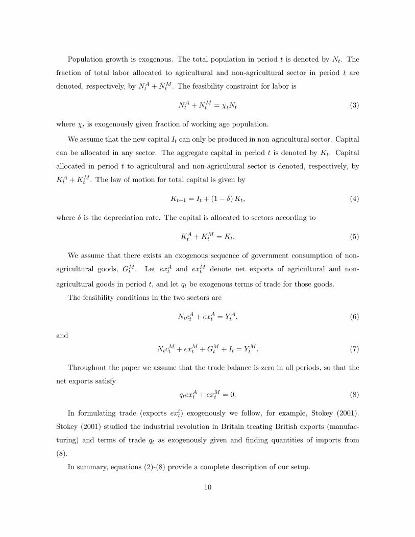
Population growth is exogenous. The total population in period t is denoted by Nt. The

fraction of total labor allocated to agricultural and non-agricultural sector in period t are

denoted, respectively, by NAt +N

Mt . The feasibility constraint for labor is

NAt +N

Mt = �tNt (3)

where �t is exogenously given fraction of working age population.

We assume that the new capital It can only be produced in non-agricultural sector. Capital

can be allocated in any sector. The aggregate capital in period t is denoted by Kt. Capital

allocated in period t to agricultural and non-agricultural sector is denoted, respectively, by

KAt +K

Mt . The law of motion for total capital is given by

Kt+1 = It + (1� �)Kt; (4)

where � is the depreciation rate. The capital is allocated to sectors according to

KAt +K

Mt = Kt: (5)

We assume that there exists an exogenous sequence of government consumption of non-

agricultural goods, GMt . Let exAt and exMt denote net exports of agricultural and non-

agricultural goods in period t, and let qt be exogenous terms of trade for those goods.

The feasibility conditions in the two sectors are

NtcAt + ex

At = Y

At ; (6)

and

NtcMt + exMt +GMt + It = Y

Mt : (7)

Throughout the paper we assume that the trade balance is zero in all periods, so that the

net exports satisfy

qtexAt + ex

Mt = 0: (8)

In formulating trade (exports exit) exogenously we follow, for example, Stokey (2001).

Stokey (2001) studied the industrial revolution in Britain treating British exports (manufac-

turing) and terms of trade qt as exogenously given and �nding quantities of imports from

(8).

In summary, equations (2)-(8) provide a complete description of our setup.

10

3.2 Frictionless benchmark

We proceed now to characterize a standard social planner�s problem. The optimality conditions

are as follows:

the intratemporal capital allocation condition across sectors is given by

1 =UMc;t

UAc;t

FMK;t

FAK;t; (9)

the intratemporal labor allocation condition is given by

1 =UMc;t

UAc;t

FMN;t

FAN;t; (10)

and the intertemporal (Euler) condition is given by

1=�1 + FMK;t+1 � �

��UMc;t+1

UMc;t: (11)

The solution to this social planner�s problem coincides with and can be decentralized as

competitive equilibrium. We omit the formal de�nition of the competitive equilibrium as it

is standard. In the competitive equilibrium all agents pool their income and maximize their

utility (2) subject to a budget constraint in each period

pAt NtcAt +Ntc

Mt +KA

t+1 +KMt+1

= wAt NAt + w

Mt N

Mt +

�1 + rAt � �

�KAt +

�1 + rMt � �

�KMt +�Mt +�At � Tt;

where wit; rit;�

it are, respectively, the wage, the rate of return on capital, and the pro�t in

sector i; pAt is the price of agricultural goods in terms of non-agricultural goods; and Tt is the

lump sum taxes.

Firms in sector i hire capital and labor to maximize pro�ts

�it = maxfKi

t ;NitgpitA

it

�Kit

��K;i �N it

��N;i � witN it � ritKi

t ;

where pMt = 1.

Maximization behavior of the �rms implies that wit and rit are equal to the marginal product

of capital and labor in sector i in each period. Maximization behavior of consumer implies

that wit and rit are equalized across sectors.

We will show that data rejects the implications of this frictionless competitive equilibrium.

11

3.3 Wedges accounting

Our description of Russian economy showed a large number of institutional frictions and gov-

ernment policies that distorted households and �rms decisions. Modeling each of these frictions

explicitly is di¢ cult as there was a large number of such frictions, and because there is not

enough data to realistically estimate the magnitude of each of them. Instead we follow a di¤er-

ent path. We use the insights of Cole and Ohanian (2004) and Chari, Kehoe and McGrattan

(2007) that any policies can be mapped into wedges in a prototype competitive equilibrium

model. Policies and frictions manifest themselves in di¤erent wedges, and by studying these

wedges we can identify likely sources of these distortions.

Speci�cally, we de�ne three wedges, each equal to deviations in the right hand side of

equations (9), (10), and (11) from 1. These three wedges correspond to the intratemporal

distortions in capital and labor allocations between sectors and to the intertemporal distortion.

In addition to these three wedges, we also explicitly focus on one of the most important

Stalin�s economic policies � price scissors, discussed in Section 2. This policy introduces a

wedge between the relative prices that producer of agricultural goods faces, and the prices

that consumers are willing to pay. Speci�cally, if producer of agricultural goods faces a price

pA;t and consumer faces a price ~pA;t; then the price scissor wedge, 1+�C;t; is given by 1+�C;t =

~pA;t=pA;t =UAc;t

pA;tUMc;t: Thus, using additional data on the producer relative prices (for the �rst

three wedges), we de�ne four wedges, �R;t; �W;t; �C;t and �K;t+1 as follows

1 + �R;t �FMK;t

pA;tFAK;t=rMtrAt; (12)

1 + �W;t =FMN;t

pA;tFAN;t=wMtwAt

;

1 + �C;t =UAc;t

pA;tUMc;t;

1 + �K;t+1 =�1 + FMK;t+1 � �

� �UMc;t+1UMc;t

:

Note that the intratemporal distortions for capital and labor implied by the right hand

side of expressions (9) and (10) are given by (1 + �R;t) = (1 + �C;t) and (1 + �W;t) = (1 + �C;t).

These normalized wedges (as well as the intertemporal wedge) do not require knowledge of the

prices.

12

The normalized intratemporal labor wedge, for example, implies that reduction is misal-

location of labor between agriculture and manufacturing can be achieved either by reducing

the wedge �W;t; which is determined by the ratio of the wages paid in the two sectors and in

many models is often related to the size of barriers to labor mobility or by increasing �C;t;

which measures distortions between consumer and producer prices. This distinction helps us

to evaluate the e¤ect of di¤erent policies.

Additionally, one can also think of�AMt ; A

At ; ex

it; G

Mt

Tt=0

also as wedges. We want to em-

phasize that our analysis is essentially an accounting procedure. Given initial K0, competitive

equilibrium allocations with wedges�AMt ; A

At ; �R;t; �W;t; �C;t; �K;t; ex

it; G

Mt

Tt=0

match data ex-

actly. This allows to compute the marginal contribution of each wedge to the deviations of

data from undistorted allocations.

4 Data and calibration

In this section we discuss the construction of the data for a systematic comparison of the

structural transformation during Stalin years and during tsarist years.12 To our knowledge

this comprehensive construction of the data is novel as most importantly it details the sectoral

variables, calculation of capital series, and recalculation of GDP in market prices of 1913.

4.1 Data sources and construction of the data

The principal source of economic data for output, consumption and investments for Russia in

1885-1913 is Gregory (1982). Gregory compiled data on net national income and its component

using a variety of historical sources, most of which coming from the o¢ cial tsarist statistical

publications. His data is su¢ ciently disaggregated and allows us to construct series for con-

sumption and investments for agricultural and non-agricultural sector and to use a perpetual

inventory method to impute capital stock. Unfortunately, he does not provide enough inform-

ation to separate residential housing stock and non-residential capital in agriculture. This

leaves us no choice but to include rural residential housing stock in our measure of agricultural

capital. For the reasons explained in the Appendix, we exclude urban residential capital from

any measure of capital stock. The data on value added by sector is scanter �we have those

estimates only for a few select years.12We refer the reader to the Appendix for the complete treatment.

13

We obtain Soviet economic data from Moorsteen and Powell (1966). They use o¢ cial

Soviet data to construct sectoral outputs, capital stock, and value added according to Western

de�nition. Although the o¢ cial price series may not be representative of true market clearing

prices, there seems to be a consensus among economic historians that the underlying quantities

are generally reliable (see, e.g., a discussion in Appendix A of Allen 2003). Using data in

Moorsteen and Powell (1966), as well as additional data from Allen (1997), Davies (1990), and

Davies et. al. (1994) we compile sectoral outputs, investment, capital stock, and consumption

for agricultural and non-agricultural sectors in Soviet 1937 prices. To convert these values to

1913 prices, we use Markevich and Harrison (2011) estimates of Soviet sectoral value added in

1928 in 1913 prices. That is, we implicitly assume that intra-sectoral prices remain unchanged,

and infer sectoral relative price conversion from their data. The details are in the Appendix.

Since the role of government changed dramatically between 1913 and 1928, we de�ne gov-

ernment purchases narrowly as military spending. We count all other government expenditures

as non-agricultural consumption.

Calculating sectoral employment or even the labor force is di¢ cult both for tsarist and for

Soviet periods. Unlike data on economic aggregates, there is little reliable data on sectoral

employment before 1913. Tsarist Russia conducted only one national census in 1897. There

are employment records from the administrative data in some heavy industries but for the

rest of the economy there are only sporadic surveys. For this reason Gregory (1982) does not

provide annual employment numbers but only his estimates of growth rates of labor force for

agriculture, manufacturing and services for 1883-87 to 1897-1901 and for 1883-1897 to 1909-

1913. An early Soviet economic historian Gukhman used census and archival data to estimate

composition of labor force in 1913, which was then reproduced in Davies (1990). As in census

as well as Gukhman and Davies, we de�ne sectoral employment for each worker according to

self-reported primary occupation. This de�nition seems to be the only way to obtain a con-

sistent de�nition of sectoral labor force for tsarist Russia, Soviet Union, and Japan. It almost

certainly overestimates the true employment in agriculture and underestimates employment in

manufacturing. There is substantial evidence that agricultural workers spent a part of their

time in non-agricultural activities, such as seasonal manufacturing work in the city and self-

employed promysly. As a robustness check, we recompute our wedges under assumption that

10 percent of time of agricultural workers is spent on non-agricultural activities, which is con-

14

sistent with estimates of Moorsteen and Powell (1966) for the Soviet period. The results of

this robustness check are reported in the online appendix.

We also need to take a stand on how to treat employment of women. The available employ-

ment records before 1913 are from select heavy industries which predominantly employed men.

As non-agricultural sector expanded dramatically after 1928, so did the fraction of women in

non-agricultural employment. Based on this evidence one may be tempted to conclude that

female labor force participation signi�cantly increased. At the same time, there is evidence

that before 1913 female labor force participation in agriculture was very high, as women had

to replace men who were employed as migrant workers in urban industries. For example, Crisp

(1978) in her study of Russian labor markets pre-WWI points out that although in factory

industry there were only 800,000 women compared to several million men, in peasant farms

"the proportion of women undoubtedly exceeded that of male, especially if all-year-around

averages are taken into account". Since there are no reliable �gures about female labor force

participation, we do not treat women and men di¤erently and assume that all working age

population is a part of the labor force.

We have data series for real GDP growth in 1913 rubles for Russia. We also have real

GDP in 1990 international dollars for 1913. To construct real GDP per capital, we use real

GDP per capita in international dollars for 1913, and then apply real GDP growth rates (in

constant rubles and dollars) to construct real GDP in international dollars for other years in

1885-1913. This series may di¤er slightly from real GDP in international dollars for other years

as relative prices might have changed. However, our index captures well the general patterns.

The fraction of agricultural value added measures the ratio of agricultural value added in 1913

prices to real GDP in 1913 prices. Sectoral net imports and exports are shown relative to the

sectoral value added.

4.2 Summary of the data

Figures 2 and 3 show aggregate and sectoral, agricultural and non-agricultural, data for both

tsarist and Soviet Russia.

15

4.2.1 1885-1913

Russian economy in 1885-1913 grew rather signi�cantly, with the average rate of growth of

real GDP per capita of 1.91 percent. However, the economy did not experience structural

transformation from agriculture. About 85 percent of working age Russian population have

their primary occupation in agriculture in 1885, and this fraction declines very slowly, only

to 81 percent in 1913. The role of agriculture in the economy was also very important, with

about 53 percent of value added being produced in agriculture in 1885, declining only to 46

percent in 1913. International trade was rather important �tsarist Russia exported about 10

percent of its agricultural production, and imported primarily manufacturing goods.

4.2.2 Soviet Russia (1928-1940)

The level of GDP per capita and the structural composition of Russian economy in 1928 is

approximately the same as it was in 1913.13 This re�ects the years of turmoil following the

fall of tsarist Russia and the subsequent years under the communist rule.

We now turn to Russia in 1928-1940. Growth in real GDP (measured in 1913 rubles) is

very rapid. This coincides with a rapid increase in investments and reallocation of labor from

agriculture to non-agriculture.

The bottom row shows agricultural and non-agricultural per capita value added in 1913

prices, capital stock, and government expenditures. Non-agricultural value added shows re-

markable growth. Agricultural value added drops during collectivization in 1928-1933 then

returns towards its trend. The capital stock in 1928 is approximately the same in agriculture

as it was in 1913, and is signi�cantly smaller in non-agriculture. The military expenditures

in Soviet Russia were generally low in the late 1920s and early 1930s followed by a signi�cant

military build up starting from mid 1930s.

A special discussion of price series is needed for Soviet Russia. While in market economies

various price series (e.g. retail, wholesale prices or o¢ cial procurement prices) are highly

correlated, it is not the case for the Soviet Russia. After 1928 there is a host of di¤erent

13We do not report the data for Tsarist Russia during World War I (1914-1917) or for the period followingFebruary Revolution (1917) to 1927. This period covers October (Bolshevik) Revolution, the Civil War, WarCommunism, and the New Economic Policy (NEP). The main reason is that the issues of availability andquality of the data do not allow us to construct the dataset comparable to the one we constructed. Even thoughMarkevich and Harrison (2011) provide many time series for this period, there is still no data on capital. Thatis why, we are not able to estimate TFP and wedges for those periods.

16

1890 1900 1910 1920 1930 1940500

1000

1500

2000

2500

3000Real GDP per capita

PP

P 1

990 

inte

rnat

iona

l dol

lars

1890 1900 1910 1920 1930 19400.3

0.4

0.5

0.6

0.7

0.8

0.9Labor Share in Agriculture

1890 1900 1910 1920 1930 19400.1

0.2

0.3

0.4

0.5

0.6

Agric Value Added to GDP in 1913 prices

1890 1900 1910 1920 1930 19400

0.05

0.1

0.15

0.2

0.25

0.3

Investment to GDP ratio

1890 1900 1910 1920 1930 19400.2

0.4

0.6

0.8

1

1.2

1.4

1.6

pA

/pM

1890 1900 1910 1920 1930 19400

0.05

0.1

0.15

0.2Import and Export to GDP ratios

exA

/YA

­exM

/YM

Figure 2: Aggregate economic indicators in Russia in 1885-1940.

1890 1900 1910 1920 1930 19400.8

1

1.2

1.4

1.6

1.8

2

2.2Capital to Value Added ratios

1890 1900 1910 1920 1930 19400

0.2

0.4

0.6

0.8

1

1.2

1.4Value Added to GDP ratios

1890 1900 1910 1920 1930 19400

0.02

0.04

0.06

0.08

0.1Government to GDP ratio

1890 1900 1910 1920 1930 19400

0.2

0.4

0.6

0.8

1Consumption to GDP ratios

1890 1900 1910 1920 1930 1940100

110

120

130

140

150

160

170

180Population

KA

/YA

KM

/YM

YA

/GDP1913

YM

/GDP1913

CA

/GDP1913

CM

/GDP1913

Figure 3: Sectoral economic indicators, government and population in Russia.

17

o¢ cial prices set by the state which often diverge substantially from each other. For most of

our analysis this is not an issue since we measure quantities in 1913 prices. Price information

is needed only to construct the price scissor wedge �C;t:14 This wedge captures the terms of

trade for the producer of agricultural goods. We follow Allen (1997) and de�ne this relative

price as a ratio of o¢ cial procurement prices of agricultural goods relative to the free retail

non-agricultural consumption basket. Allen argues that this is the best measure to capture

the terms of trade that a private agricultural producer faced after 1928.

4.3 Calibration

To calibrate the model we need to choose values of eight parameters and the initial value

of capital. Technology parameters include the elasticities of production functions in the ag-

ricultural and manufacturing sectors, (�Ki; �Ni), and the depreciation rate, �. Preference

parameters include the discount factor, �, the asymptotic agricultural consumption share, �,

and the subsistence level in agriculture, A.

Some parameters that we choose are rather uncontroversial, we draw on Hayashi and

Prescott (2008) for them and provide extensive robustness in the Appendix. The depreciation

rate is set to � = 0:05, and the discount factor is set to � = 0:96: The asymptotic consump-

tion shares of agricultural and non-agricultural goods are set to � = 0:15 and 1 � � = 0:85

correspondingly. One di¤erence between our model and the model of Hayashi and Prescott is

that we do not have intermediate goods. We account for this di¤erence by assuming that all

intermediate goods used in the production of manufacturing goods represent labor. We set

the corresponding factor shares for the manufacturing sector to �K;M = 0:3 and �N;M = 0:7.

Instead, we assume that all intermediate goods used in the production of agricultural goods rep-

resent land. We set the remaining capital and labor shares to �K;A = 0:14 and �N;A = 0:55.

The values for these parameters are also similar to values adopted by Caselli and Coleman

(2001) calibrated using direct estimates for the U.S. economy.15

We choose the initial capital stock to match the observed level of capital in 1885. We do not

have data needed to directly determine the subsistence parameter, A. We set the subsistence

level to 28 rubles per capita per year in 1913 prices. This subsistence level accounts for 72

14Prices also feature in our de�nitions of �W;t and �R;t: The prices drop out, however, if we consider normalizedintra-sectoral labor and capital distortions, (1 + �W;t) = (1 + �C;t) and (1 + �R;t) = (1 + �C;t) :15Caselli and Coleman (2001) use the values �K;M = 0:6, �N;M = 0:34, �K;A = 0:21 and �N;A = 0:6.

18

percent of agricultural consumption per capita in 1885. If we were to set it higher than

81 percent of consumption of 1885 the simulated economy would go below the subsistence

level during tsarist years. As we discuss in the online appendix, our main results are robust

to alternative values of A below this value. Finally, for �t; the fraction of labor force in

population we set �t = 0:53 for all t; which is the fraction in the Russian census of 1897. This

number is slightly higher than fraction of labor force from 1926 and 1939 censuses, but �tting

those numbers produce only small di¤erences for the analysis.

5 Wedges

We now proceed with the calibrated model to compute wedges using equation (12)16. Figure

4 shows wedges for Russia with solid lines and their average level (or trends, for the case of

TFPs) with dashed lines.

1890 1900 1910 1920 1930 19400.8

1

1.2

1.4

1.6

1.8

AM

WedgeTrend

1890 1900 1910 1920 1930 19400.8

1

1.2

1.4

1.6

1.8

2

2.2

AA

WedgeTrend

1890 1900 1910 1920 1930 1940­2

0

2

4

6

8

10

12

τC

WedgeTrend

1890 1900 1910 1920 1930 19400

5

10

15

20

25

τW

WedgeTrend

1890 1900 1910 1920 1930 19400

2

4

6

8

10

12

τR

WedgeTrend

1890 1900 1910 1920 1930 1940­0.2

0

0.2

0.4

0.6

0.8

τK

WedgeTrend

Figure 4: Russia: Wedges vs. Trends based on pre-1913 simulation.

The behavior of the wedges can be grouped in three main periods. The �rst is tsarist

Russia (1885-1913). The second is the initial period of industrialization and collectivization16The wedge �K;t can only be computed up to 1939 using available data. Wedge �K;1940 is determined by

the expected consumption in 1941, for which we do not have data. To impute �K;1940 we assume that expectedconsumption growth in 1940 is the average of expected consumption growths in 1937-1940.

19

(1928-1935) when the wedges exhibited dramatic changes. The third period is that of the

stabilization of wedges (1936-1940) that ends with the entry of Russia into the WWII .17 We

present the average wedges for di¤erent periods in Table 4 in the appendix.

5.1 Wedges in 1886-1913 (Tsarist Russia)

The �rst period is tsarist Russia. The TFP and the wedges exhibit some �uctuations and noise

but are certainly less variable than during Stalin�s period. The average TFP annual growth is

1.45 percent is agriculture and 0.66 percent in non-agriculture. The four wedges de�ned in (12)

are noisy but do not exhibit any trend in 1885-1913. Observing these wedges it becomes evident

that Russia faced signi�cant distortions in its economy. The average normalized intratemporal

(inter-sector) labor wedge, (1 + �W;t) = (1 + �C;t), is equal to 5.9. The average normalized

intratemporal (inter-sector) capital wedge, (1 + �R;t) = (1 + �C;t), is equal to 2.4. The average

intertemporal (investment) wedge is equal to 0.11. The average size of the intratemporal labor

wedge in Russia is higher than in Caselli and Coleman (2001) who report the ratio of the farm

wage to the manufacturing wage to be 0.20 in the USA in 1880, so that the wedge is equal to

4.

Connecting wedges to the policies/distortions

Intratemporal labor wedge. The large size of the intratemporal labor wedge stands out. This

is consistent with the view of Gerhenkron (1962) that the unusually slow decline of the share

of agriculture in GDP in Tsarist Russia can be explained by the barriers to the rural-urban

migration, in particular, by the institutions of obschina. This institution of obschina e¤ectively

prescribed communal ownership of land and existed in 38 out of 50 European provinces of

Russia (Chernina et al., 2011). In other provinces either there were no communes or those

were hereditary communes (with individual ownership of land). The hereditary commune

allowed for exit � as long as the exiting individual or household could sell to an individual

or household within the commune. In the repartition communes (peredelnaya obschina), exit

required the consent of the commune; there was no right to sell land and get compensation. At

the beginning of the twentieth century most of the peasant households lived in the commune

17Davies (1998) adopts a slightly more nuanced view of the sub-phases of economic development in 1928-41:1928-30; 1930 spring/summer-1932; 1933; 1934-1936; 1937-June 22, 1941. His description of the periods up toand including 1933 �ts our initial period identically. We could have started "stabilization period" from 1934.However, we view 1934-1935 as the recovery from the low base of the disaster of the initial phase of Stalinpolicies. Starting stabilization period from 1935 (rather than 1936) changes our results only insigni�cantly.

20

(Davies 1998, p. 8).

There was another feature of the communal land ownership in Russia that was particu-

larly important: the individual peasant strips were subject to repartition and redistribution.

This temporary character of land ownership, as argued by Gershenkron (1965), signi�cantly

decreased incentives to improve the land or invest in it. In our setup, this aspect of obschina

likely represents itself in the low agricultural TFP levels and growth rates.

Reforms of Witte and Stolypin and the behavior of the wedges. Several issues with the

structure of the tsarist economy and the policies are also important to note.18 The study of

Von Laue (1963) on Finance Minister Sergei Witte, shows how he persuaded the Tsar Nicholas

II that state-encouraged industrialization was needed for the survival of the political regime.

The main elements of the Witte�s reform were: an introduction of gold standard, state support

(signi�cant allocations from the state budget to build the railroads) and �nancing for expand-

ing the railway network (the state arranged and guaranteed foreign loans), encouragement of

foreign investment (especially in the iron and steel industries). Von Laue�s and Gerhenkron�s

(Gerhenkron 1965) opinion was that the state played an important role in Russia�s industri-

alization. This view was challenged in an in�uential study by Kahan (1967) who argued that

the taxes and other state intervention, as well as introduction of the gold standard, outweighed

the bene�ts of the state interventions. Our calculation of the wedges does not give a clear an-

swer and the resolution to these debates. Likely, there is truth in both sides of the argument.

What we take from this debate is that there were likely very signi�cant distortions to �nancing

that necessitated state�s involvement either through facilitating loans or channeling resources

in construction of railroads and in encouraging foreign investment in heavy industries that

we discuss next. These �nancial frictions coupled with generally low level of development of

Russian �nancial markets lead us to believe that the intertemporal wedge that we �nd in our

analysis was indeed quite signi�cant.

Following the revolution of 1905, tsarist government started a major agrarian reform. The

Prime Minister Stolypin�s reform (a series of decrees issued in 1906-1910) allowed individual

sales of land and greatly facilitated exit from the repartition communes. The main goal of the

policy was encouragement of the villagers to leave the commune and establish their separate

18The discussion of the literature and the assemsent of the state of the debate that follows in this section isbased on an excellent summary of the tsarist economy in the book by Davies (1998).

21

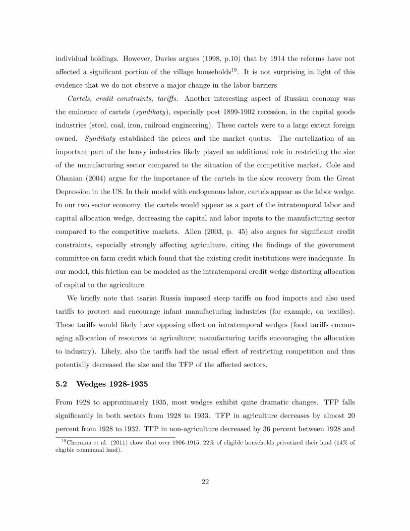
individual holdings. However, Davies argues (1998, p.10) that by 1914 the reforms have not

a¤ected a signi�cant portion of the village households19. It is not surprising in light of this

evidence that we do not observe a major change in the labor barriers.

Cartels, credit constraints, tari¤s. Another interesting aspect of Russian economy was

the eminence of cartels (syndikaty), especially post 1899-1902 recession, in the capital goods

industries (steel, coal, iron, railroad engineering). These cartels were to a large extent foreign

owned. Syndikaty established the prices and the market quotas. The cartelization of an

important part of the heavy industries likely played an additional role in restricting the size

of the manufacturing sector compared to the situation of the competitive market. Cole and

Ohanian (2004) argue for the importance of the cartels in the slow recovery from the Great

Depression in the US. In their model with endogenous labor, cartels appear as the labor wedge.

In our two sector economy, the cartels would appear as a part of the intratemporal labor and

capital allocation wedge, decreasing the capital and labor inputs to the manufacturing sector

compared to the competitive markets. Allen (2003, p. 45) also argues for signi�cant credit

constraints, especially strongly a¤ecting agriculture, citing the �ndings of the government

committee on farm credit which found that the existing credit institutions were inadequate. In

our model, this friction can be modeled as the intratemporal credit wedge distorting allocation

of capital to the agriculture.

We brie�y note that tsarist Russia imposed steep tari¤s on food imports and also used

tari¤s to protect and encourage infant manufacturing industries (for example, on textiles).

These tari¤s would likely have opposing e¤ect on intratemporal wedges (food tari¤s encour-

aging allocation of resources to agriculture; manufacturing tari¤s encouraging the allocation

to industry). Likely, also the tari¤s had the usual e¤ect of restricting competition and thus

potentially decreased the size and the TFP of the a¤ected sectors.

5.2 Wedges 1928-1935

From 1928 to approximately 1935, most wedges exhibit quite dramatic changes. TFP falls

signi�cantly in both sectors from 1928 to 1933. TFP in agriculture decreases by almost 20

percent from 1928 to 1932. TFP in non-agriculture decreased by 36 percent between 1928 and

19Chernina et al. (2011) show that over 1906-1915, 22% of eligible households privatized their land (14% ofeligible communal land).

22

1933. The TFP then bounces back but reaches the level of 1928 only in 1934 for agriculture,

but in manufacturing does not achieve the level of 1928 TFP even by 1940.

Wedges �R;t; �W;t and �C;t also follow the same patterns, �rst increasing dramatically,

then decreasing. The peak of all increase coincides with the peak of collectivization policies.

From 1928 to 1932 we observe the following behavior of the wedges. The price scissor wedge

jumps tenfold. The intrasectoral labor wedge and the intrasectoral capital wedge double. The

normalized labor wedge decreased tenfold and the normalized intersector capital wedge almost

became zero. There is no discernible pattern in terms of the intertemporal capital wedge.

To understand this pattern, it is useful to think about the implications for wedge decom-

position of the behavior of the sectoral data in Figure 2. This �gure shows a substantial drop

in agricultural output, together with substantial reallocation of labor force from agriculture

to non-agriculture. This coincides with a substantial decrease in pA;t=pM;t ratio, which is con-

sistent with the policy of price scissors. The response of the economy under Stalin�s policy

to a drop in agricultural output is exactly the opposite from the predictions of a frictionless

neoclassical growth model. In the frictionless two sector growth model non-homotheticity in

consumption of agricultural goods implies that in response to a drop in agricultural TFP (and,

hence, a fall in production and consumption of agricultural goods) relative prices of agricul-

tural goods increase by more than the fall in TFP. This creates incentives to reallocate labor

into agriculture to increase the output of food which became more valuable. Stalin�s policy of

price scissors led to the opposite e¤ect. By keeping producer prices of agriculture arti�cially

low, he created incentive for labor to move from agriculture, exacerbating the food problem.

The e¤ect of price scissors is so large that the labor wedge �W;t had to increase to partially

o¤set the e¤ect of price scissors.

Connecting wedges to the policies

We now further elaborate on the connection of the policies to the wedges20.

We �rst note that it is not surprising that the wedges change dramatically during those

periods and that the wedges �uctuate so signi�cantly. The policies of industrialization and

collectivization were overwhelmingly signi�cant and at the same time quite erratic. In 1929,

the drive to collectivize started with exceptionally ambitious plans to completely restructure

the economy. Stalin calls 1929 the year of the Great Break (Stalin, November 7, 1929) and

20For a signi�cant part of the discussion here, we follow Davies, et al 1994.

23

a �decisive advance�on the way to industrialization �leaving behind Russian backwardness�.

On March 2, 1930 Stalin publishes an article in Pravda "Dizziness from Successes", signifying

a partial retreat from the �rst push of collectivization. Davies (p. 15-17 in Davies, et. al 1994)

describes the 1928-1930�s period as that of "Utopian concepts of the emerging socialist order

prevailing in o¢ cial circles", period of Spring/Summer 1930-summer 1932 as that when period

of "economic policy and practice were confused and ambitious" with greater realism settling

in, and only by late 1933 the realism (but not the brutality of the policies) prevails.

Policies and the fall in agricultural TFP. We now proceed to describe evidence that is

consistent with the drastic fall of the agricultural TFP that we observe in the data. We argue,

that while TFP is often thought as exogenous, Stalin�s policies were the likely culprit behind

the �endogenous� fall in TFP. Davies and Wheatcroft (Chapter 6 in Davies, et. al. 1994)

describe key factors a¤ecting agricultural production in these years. First, the state exaction

of grain from peasants on its own created dramatic disruption in agricultural production. There

was virtually no incentives to work on the collectivized land. The system of crop rotation was

severely disrupted and not restored even by 1935 when crop rotation was used only on 50

percent of the sown area. The grain requisition led to a drastic fall in livestock because of

lack of food. This fall in quantity, exacerbated by the careless application of the available

manure, in turn led to a signi�cant reduction of manure to fertilize the land and again lowered

its productivity. Second, the dekulakization campaign of 1929-1931 a¤ected �ve to six million

peasants, one million out of 25 million peasant households (Wheatcroft and Davies, p. 68 in

Davies et al 1994). These most successful and knowledgeable peasants were in the best case

exiled, and in the worst case executed. Third, there was a signi�cant decline in skills and

technical training. A part of this can be attributed to dekulakization itself. Another part

was due to the lack of experience on the side of the urban workers who were sent to run the

collectivized farms. Additionally, the purges of the "bourgeois" elements bled the agricultural

(as well as non-agricultural) sector of the trained specialists. Fourth, the system of centralized

control and planning led to a variety of erroneous decisions made. Neither Stalin and the

top brass of the Soviet elite, nor the regional party secretaries had experience in agriculture.

Wheatcroft and Davies (p. 124 in Davies et al 1994) argue that the positive elements of

the centralized planning (economy of scale, some new advanced farming methods, increase in

mechanization, etc.) were outweighed by the "great disadvantages ... from the ignorance of

24

politicians". Finally, as mentioned above the fall in livestock itself decreased productivity.

Partially, within the con�nes of the model the fall in the livestock resulted in decrease in the

agricultural capital. However, horses were also used as the main draught power and the decline

in number of horses signi�cantly worsened the productivity of agriculture. By July 1933, the

available horsepower dropped to 16 million horses from 27 million in 1928. The tractors

in 1933 only amounted to 3.6-5.4 million horsepower equivalents. These �ve key factors very

much coincide with the assessment of Nove (1992, p. 176) who concludes that the "... peasants

were demoralized. Collective farms were ine¢ cient.. [there were] appallingly low standards of

husbandry with 13 percent of the crop remaining unharvested as late as mid-September in the

Ukraine, and some of the sowing delayed till after June 1". For completeness, we also mention

that one exogenous factor in the agricultural TFP is weather. However, Wheatcroft and Davis

(p. 128 in Davies et al 1994) argue that throughout 1930s, weather was not a major factor

behind low agricultural yields and certainly much smaller factor than the policies.

Price scissors and the labor wedge. As discussed in Sah and Stiglitz (1984) and Allen

(2003), price scissors were an important policy for expropriating the �agricultural surplus�.

The state forced the peasants to sell the agricultural output at prices which were substantially

below the prices for the same output in cities.

The magnitude of price scissors was substantial. Based on Barsov (1969), Ellman (1975,

Table 6) shows that black market prices for grain were more than twice as high as the state

procurement prices in 1929. In 1930, the di¤erence was 4.5 times, in 1931 � 7 times, and

in 1932 �28 times! This mechanism is consistent with the traditional historical narrative of

collectivization (see, e.g. Conquest, 1986). The consensus is that the price scissors policies

certainly went too far even for their own sake. Millar (1974) calls these policies an �unmitig-

ated economic policy disaster�: attempting to expropriate agricultural surplus, price scissors

and mass collectivization destroyed the surplus resulting in the decline of agricultural output

and eventually a great famine (costing several millions of lives). Millar argues that the food

production declined so much that peasants slaughtered livestock decreasing the traction power

(see the numbers above); instead of investing in industrial capital stock, the state had to pro-

duce or import tractors for restoring the traction power. This further reduced net agricultural

surplus.

However, the huge decrease in rural living standard did accelerate rural-urban migration.

25

As Davies and Wheatcroft (2004) note �by the autumn of 1932 peasants were moving to the

towns in search of food.�The growth of urban population ceased, and was partially reversed,

only as a result of restrictions on movement and the introduction of an internal passport

system�(p. 407). The introduction of the passport system can be viewed as providing evidence

for the increase in the labor wedge that we already discussed.

Realizing the fact that price scissors were too high, after 1932 the government decreased

them substantially. Moreover, in 1932, the state legalized agricultural markets (so called

collective farm markets, kolkhoznye rynki) where peasants could freely sell output that they

produced in excess of their planned delivery quotas; the quotas were also relaxed (Davies et

al., 1994, p.16). This allowed the peasants to reap at least some bene�ts of the high market

prices for food but also reduced incentives to migrate to the cities.

Policies and the non-agricultural TFP.We now turn to the behavior of the non-agricultural

TFP21. Some factors that we already described in the case of the fall and �uctuations of

agricultural TFP are also relevant for the case of the non-agricultural TFP, speci�cally, wild

swings in policies and the repression against "bourgeois" specialists. We now present other

evidence supporting our �ndings of the impact of Stalin policies on the non-agricultural TFP

during those years. We also discussed already the fall in the number of horses and the urgent

need to produce tractors. This led to ine¢ cient and rush diversion of resources to industries

producing mechanized equipment from agriculture. Davies (p.153) argues that in 1932 half

of the high quality steel produced in the country was used in production of tractors. The

capacity of iron and steel plants diverted to tractors could be used to �nish the overambitious

construction projects started earlier. The food crisis of 1932-1933 also forced to reduce the

number of workers in construction. In other words, both the price scissors and the fall in

agricultural TFP also represented themselves in the fall of non-agricultural TFP. This initial

period of industrialization did indeed bring importation of the foreign technology and practices

but it was still quite limited (we expand on this in the next section) and unlikely to a¤ect the

non-agricultural TFP signi�cantly at the aggregate level.

An important factor was the overall poor quality of the workers moving from agriculture.

Nove (1992, p. 198-199) details the issue and argues that outside the machinery and the metal-

21We closely follow the discussion of the chapter "Industry" by Davies in Davies, et. al. 1994. All pages referto that chapter unless otherwise noted.

26

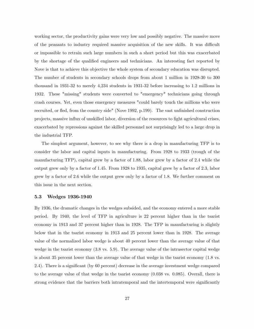
working sector, the productivity gains were very low and possibly negative. The massive move

of the peasants to industry required massive acquisition of the new skills. It was di¢ cult

or impossible to retrain such large numbers in such a short period but this was exacerbated

by the shortage of the quali�ed engineers and technicians. An interesting fact reported by

Nove is that to achieve this objective the whole system of secondary education was disrupted.

The number of students in secondary schools drops from about 1 million in 1928-30 to 300

thousand in 1931-32 to merely 4,234 students in 1931-32 before increasing to 1.2 millions in

1932. These "missing" students were converted to "emergency" technicians going through

crash courses. Yet, even those emergency measures "could barely touch the millions who were

recruited, or �ed, from the country side" (Nove 1992, p.199). The vast un�nished construction

projects, massive in�ux of unskilled labor, diversion of the resources to �ght agricultural crises,

exacerbated by repressions against the skilled personnel not surprisingly led to a large drop in

the industrial TFP.

The simplest argument, however, to see why there is a drop in manufacturing TFP is to

consider the labor and capital inputs in manufacturing. From 1928 to 1933 (trough of the

manufacturing TFP), capital grew by a factor of 1.88, labor grew by a factor of 2.4 while the

output grew only by a factor of 1.45. From 1928 to 1935, capital grew by a factor of 2.3, labor

grew by a factor of 2.6 while the output grew only by a factor of 1.8. We further comment on

this issue in the next section.

5.3 Wedges 1936-1940

By 1936, the dramatic changes in the wedges subsided, and the economy entered a more stable

period. By 1940, the level of TFP in agriculture is 22 percent higher than in the tsarist

economy in 1913 and 37 percent higher than in 1928. The TFP in manufacturing is slightly

below that in the tsarist economy in 1913 and 25 percent lower than in 1928. The average

value of the normalized labor wedge is about 40 percent lower than the average value of that

wedge in the tsarist economy (3.8 vs. 5.9). The average value of the intrasector capital wedge

is about 35 percent lower than the average value of that wedge in the tsarist economy (1.8 vs.

2.4). There is a signi�cant (by 60 percent) decrease in the average investment wedge compared

to the average value of that wedge in the tsarist economy (0.038 vs. 0.085). Overall, there is

strong evidence that the barriers both intratemporal and the intertemporal were signi�cantly

27

reduced in this period. This provides strong support to the view of Allen (2003) or Acemoglu

and Robinson (2012) that Stalin�s policies removed barriers in the Soviet economy. However,

the TFP in agriculture increased only insigni�cantly while TFP in manufacturing is lower.

Connecting wedges to the policies

Manufacturing TFP. We now continue our discussion in the previous section of why the

TFP estimates for non-agricultural sector we obtain are lower in 1940 than in 1928. The key

force is the signi�cant expansion of inputs. From 1928 to 1940, capital in non-agriculture grew

by a factor of 4.4, labor in non-agriculture grew by a factor of 3.7 while the output grew only

by a factor of 2.75. We proceed with further discussion of changes in Soviet technology which is

based on Lewis (Chapter "Industry" in Davies, et al. 1994). Our estimates of the slow growth

of TFP are consistent and are directly supported with the summary of the data by Moorsteen

and Powell, by Bergson, by Khanin, and by Seton (Lewis, p 195-196 and Figure 15, Table 41

therein). The main conclusion of these studies is that TFP growth had an insigni�cant impact

on growth compared to the growth in inputs. Moreover, Moorsteen and Powell also point out

that the TFP growth in non-agriculture was lower than in the economy as a whole.

On one hand, there were two main positive factors that led to an increase in productivity.

First, there certainly were important technological advances. The scale and e¢ ciency in many

industries signi�cantly increased (for example, the new and larger blast-furnaces in iron and

steel industry or use of explosions and pneumatic picks in coal mining). Soviet Russia was one

of technological leaders in airframe manufacturing and design of tanks. Imported technology

was introduced and became operational such as Gorkii car plant (based on Ford plant) and the

giant Magnitogorsk iron and steel combine (modeled on US Steel in Gary Indiana). By 1940,

Soviet Russia caught up with Western Europe in high energy transmission. The second positive

factor was improvement in the quality of the labor force. The peasants who joined industry in

1928 by 1940 became quite seasoned and trained workers, some became managers with years of

experience in rapid industrialization. Moreover, there was a marked increase in incentives with

campaigns on "socialist competition" and Stakhanovite movement of rewarding over-achievers

and production stars (see an extensive discussion on these improvements in labor force in Nove

1992, p. 234-235)

On the other hand, Lewis (p. 196) lists �ve key factors that support his conclusion that

"the role of technology in the Soviet growth during the years after 1928 was not as great as

28

might be assumed from a listing of the technological developments of the period". First, the

most modern technology was concentrated only in some sectors while the rest of the economy

lagged signi�cantly behind (for example: construction overwhelmingly used brick and timber

rather than concrete; steam power was still the main source of power in railways). Second,

the vertical integration developed to overcome the poor cross-industry planning led to most

of the industries and even large plants operating as self-contained empires. Many of the

inputs, related materials and spare parts were produced "in house" often ine¢ ciently and

with technology lagging behind the �agship product of those industries. Third, overmanning

of the industry was a norm. Forth, after the �rst wave of foreign technology was put in

operation there was a slowdown of import of technology and, importantly, the use of the

foreign specialist. Finally, gigantomania with the giant factories and production sites often

led to ine¢ cient application of the foreign technology designed for much smaller operations as

well as presented often insurmountable organizational and business practice projects.

Agricultural TFP. Most of the negative TFP e¤ects of the �rst wave of collectivization were

still present in this period: removal and destruction of the most productive class of peasants,

poor incentive structure to produce in the collective farms, and poor management. However,

the scale e¤ects of the large collective farms and an increase in mechanization (e.g., tractors

increased to 10.3 million hp by 1940) had their e¤ects in growing productivity.

The Great Purge and Gulag prison labor. Another factor that certainly had a negative

e¤ect on TFP (both in agriculture and manufacturing) was the terror of Great Purges22. The

peak of the repressions was the 1937-38 wave of mass arrests of members of the party and

the professional elite. Nove (1992, p. 239) argues that not only the direct e¤ect of arrests,

incarceration and executions of the managers, specialists, and civil servants were important

but also the terror imposed on the rest of the workforce were a slightest mistake or initiative

could be claimed to be act of sabotage or treason punished by death.

An important question to ask is whether forced labor was important for Stalin�s economy

and whether we should consider this separately. Recent studies (e.g., Wheatcroft and Davis in

Davies at. al. 1994 and Allen 2003, p.107-108) place the consensus number of the prisoners of

Gulag (including exiles) close to 3 million people in 1937-39. Allen (p. 108) cites Jasny (1951,

22A variety of repressions and purges were a fact of life under Stalin throughout the whole period that westudy (1928-1940), and also during the WWII and up to Stalin�s death. We already talked about the e¤ects ofthe purges of the specialists in the beginning of industrialization and of dekulakization.

29

p. 418) that "somewhat more than two concentration-camp inmates were needed to do the

work of one free laborer". He then concludes that the convicts comprised only 1.5 million "free

men equivalents" (about 2 percent of labor in the whole economy, 5 percent of the civilian,

non-farm labor) and thus "these fractions were not large enough to be decisive". As most of

these prisoners were employed in the non-skilled labor we concur with this assessment and

conclude that the main e¤ect of the Great Purge was on TFP.

Intersector labor and capital barriers. The collectivization drive succeeded in that it mostly

destroyed the institute of commune that we argued was an important factor precluding labor

mobility in tsarist Russia. Nove (1992, p. 243) concludes that by 1935 the shape of kolkhoz

as an institution was �more or less settled ... and ... remained [the same] well into sixties�.

Price scissors. As argued above, the state learned the cost of excessive price scissors and

reduced them in 1933. Through legalizing collective farm markets, government also de facto

increased the average price for grain that farmers obtained. Further more, instead of setting

the below-market procurement prices for grain, the government introduced a sales tax on food

which drove a wedge between what workers paid for food and what farmers received (Allen,

2003, p. 101). Therefore the price scissors remained but were was much lower than in the

previous period.

Big Push or Removal of Barriers. We conclude this section by stating that one of our

important �ndings is that we �nd no evidence that supports theories of the Big Push. Stalin�s

policy of industrialization and collectivization are often thought of as the �rst and the quint-

essential example of so called Big Push �a coordinated investment across interlinked sectors

undertaken by a central planner. While Allen (2003) tracks the idea of the Big Push to Soviet

economists Preobrazhensky (1965, �rst published in 1926 in Russian) and Feldman (published

in Russian in 1928), the modern concept of the Big Push was conceptualized by Rosenstein-

Rodan (1943) and formalized by Murphy, Shleifer, and Vishny (1989). The main idea of the

Big Push model is as follows. While industrialization raises aggregate output and income, it

requires coordinated decision-making across producers; in a decentralized market equilibrium,

the individually optimal choice for each �rm or household is to stick to the agrarian technology

so that industrialization does not occur. On the other hand, once the investment in industrial

technology is forced by the central planner, everybody is better-o¤. In terms of our model, the

Big Push should have shown in a signi�cant increase in TFP. However, we extensively argued

30

above that even 12 years after the start of the big push, in 1940, there is no evidence of the

signi�cantly increased TFP. If anything, Stalin�s Big Push led to a drastic drop in TFP in the

�rst years of this policy, and led to lower manufacturing TFP by 1940.

6 Russia without communist revolution: benchmark scenario

This section develops our benchmark counterfactual of how Russia would develop under al-

ternative history scenarios. In the next section, we consider other scenarios.

Our counterfactual on comparison with the tsarist economy consist of two parts. First,

we use average tsarist wedges from 1885 to 1913 and extrapolate them until 1940. We then

compare economic outcomes in that simulation to the actual performance of the economy under

Stalin in 1928-1940. Conceptually we think about this exercise as how Russian economy would

have developed if all tsarist distortions remained unchanged.23 Second, we study the question

how Russia would have developed under both Stalin and tsarist distortions after 1940 in the

absence of the WWII. One of the common arguments is that Stalin�s reforms improve economic

e¢ ciency to successfully �ght in the WWII and project economic and political dominance after

the WWII. Comparing the economic outcomes under Stalin�s and tsarist�s distortions allows

us to assess this argument.

6.1 �Tsarist�economy versus Stalin economy

For our analysis we need to take a stand on how fast population in tsarist Russia would grow.

Since we have a decreasing returns to scale technology, faster population growth leads to lower

per capita output and welfare. As Figure 3 indicates, there was a very substantial slow down in

population growth in Russia after the communist revolution of 1917, a large part of which was

caused by wars, famines, and repressions. In order to not count these towards welfare gains

for Stalin, we assume that the actual population in Russia under tsarist distortions would be

the same as population in the data.

Another issue is how to treat the initial capital stock for Stalin. As we see from Figure 3,

the capital to output ratio in 1928 was substantially below its pre-WWI trajectory. We report

23This analysis ignores a potentially destructive e¤ect of WWI which tsarist Russia would have experienced.To the extend that we can think of the war damage as a destruction of physical capital, this is not a substantialissue. If we exogenously introduce a reasonable drop in capital stock in 1918, the economy converges back toits pre-war path by 1928.

31

how our results would change if we take the economy with tsarist wedges and endow it with

Stalin�s 1928 initial capital stock.

Finally we discuss how to treat projection of Stalin�s wedges past 1940. As we have seen

from our wedge decomposition in the previous sections, Stalin�s distortions mostly stabilize

at their new levels around 1936-37. For �W;t; �R;t, �C;t we take the average values of these

variables for 1937-1940 and extrapolate them into the future. We similarly extrapolate trade

(ext, imt) and government expenditures Gt: We use a di¤erent strategy for AAt and AMt . The

growth rates of these variables ultimately drive welfare and output in the long run. From

Figure 4 one can see that it is di¢ cult to say whether there was a shift in the growth rates in

Soviet Russia in 1936-1940 compared to the tsarist economy. The TFP levels in both sectors

are lower than tsarist trend. The somewhat faster growth rate of TFP in agriculture under

Stalin could simply be a result of a catch up to the tsarist trend. For this reason we assume

that both AAt and AMt grow with tsarist trend after 1940 (the next section provides calculations

for two alternative scenarios for the projected growth rates of TFP). We take, as a starting

point for 1941, the average detrended level of AAt and AMt from 1937-1940. Finally, we chose

the level of �K;t after 1940 to ensure that the simulated model with Stalin�s wedges matches the

data exactly for 1928-1940. The resulting value of �K;t is very similar to the average pre-WWII

level of this distortion.24 The speci�cs of the projection are in Table 4 . 25

Figure 5 plots actual and projected wedges from 1928 to 1960. Figure 6 plots actual and

simulated sectoral value added, consumption, the capital stock, and the labor composition for

1928-1960. We now brie�y make several observations. Consumption of agricultural goods is

signi�cantly lower under Stalin than under the tsarist distortions in 1928-1940. Consumption

of non-agricultural goods is also signi�cantly lower except for the last several years when

non-agricultural consumption in the data is slightly higher. Since consumption is a su¢ cient

statistic for the welfare in our economy, these graphs clearly indicate that the welfare under the

Soviet distortions is signi�cantly lower than under the tsarist distortions during the 1928-1940

24We project all the wedges and simulate the economy for the period 1941-2000. We choose the terminalcondition for expected consumption in the year 2000 which implies stable rates of investment throughout theprojected period. We allow the wedges in the tsarist projection to converge to Stalin�s values between 1990 and2000. This allows us to keep the terminal condition �xed across all counterfactual exercises.25We estimate linear trends for sectoral TFPs of the Tsar and extrapolate these trends post 1913. Because

the base for the later period is higher, the implied growth rate is lower. If we estimated a log-linear rather thana linear trend for TFP, we would get unreasonably high values of GDP per capita by extrapolating the economyof the Tsar.

32

period.

The situation reverses after 1940. The lower wedges in the Stalin�s economy contribute

to a larger accumulation of capital. As a result, both the output and consumption in both

sectors under the Stalin�s distortions overtake the output and consumption under the tsarist�s

distortions soon after 1940. Therefore, the welfare becomes higher after 1940.

To formally measure the welfare gains (losses) we �nd a fraction of consumption which

needs to be added (or subtracted) to make the household indi¤erent between the simulated

consumption stream and the observed consumption stream. Thus, the welfare gain in units of

consumption, �, solves

T1Xt=T0

�tU�cAt ; c

Mt

�=

T1Xt=T0

�tU�(1 + �) cAt ; (1 + �) c

Mt

�;

where cit denotes the observed consumption streams and cit represents the simulated consump-

tion stream obtained from the counter-factual exercise.

1930 1940 1950 196070

80

90

100

110

120

130

AM

1930 1940 1950 1960150

200

250

300

350

400

AA

1930 1940 1950 19600

5

10

15

20

25

τW and τR

1930 1940 1950 19600

2

4

6

8

10

12

τC

1930 1940 1950 1960

­0.2

­0.1

0

0.1

0.2

0.3

τK

1930 1940 1950 19600

0.05

0.1

0.15

0.2

0.25

GM/YM and ex A/YA

StalinTsar

StalinTsar

τW Stalin

τR Stalin

τW Tsar

τR Tsar

StalinTsar

StalinTsar

GM/Y M Stalin

exA/Y A Stalin

GM/Y M Tsar

exA/Y A Tsar

Figure 5: Extrapolated Wedges for Stalin and Tsar

Table 1 shows decomposition of the contribution of various wedges to welfare. Speci�cally,

we start with the projected tsarist economy and replace one-by-one each tsarist wedge with

33

1930 1935 1940 1945 1950 1955 19600

50

100

150

200

250Value Added per capita

1930 1935 1940 1945 1950 1955 19600

5

10

15

20

25Capital relative to 1928

1930 1935 1940 1945 1950 1955 196020

40

60

80

100

120

140

160Consumption per capita

1930 1935 1940 1945 1950 1955 19600.5

0.6

0.7

0.8

0.9Labor Share in Agriculture

YA Stalin Y

M Stalin Y

A Tsar Y

M Tsar K

A Stalin K

M Stalin K

A Tsar K

M Tsar

cA Stalin c

M Stalin c

A Tsar c

M Tsar γ

AN

A Stalin N

A Tsar

Figure 6: Predicted Economic Indicators for Stalin and Tsar

the corresponding Stalin�s wedge in the order given in the table.26 A negative number shows

by how much the welfare decreases with the Stalin�s wedge, a positive number indicates an

increase. When we replace all tsarist wedges with their Stalin�s counterparts, we replicate data

for 1928-1940, and provide the total welfare gains. The second from the bottom line (Total)

reports the welfare numbers net of the e¤ects of population. The last line (Total net of K1928 )

reports the welfare numbers if, in addition, we assume that the tsarist economy starts with the

Soviet capital stock in 1928.

The �rst three columns correspond to welfare from 1928 to 1940 (measured as discounted

utility over those periods), to welfare from 1928 to in�nity (which represents a lifetime utility

of an in�nitely lived representative consumer born in 1928); and welfare from 1940 to in�nity

(which represents a lifetime utility of a representative consumer born in 1940). The forth

column isolates the contribution of the wedges after 1940 to the welfare after 1940. The

wedges in 1928-1940 a¤ect the welfare and the output after 1940 by a¤ecting the level of

capital, K1940: To abstract from the e¤ect of those policies, the forth column compares welfare

26Alternative decompositions give similar results.

34

under tsarist and Soviet wedges after 1940, keeping the capital stock K1940 the same for both

economies.

Our main �ndings for welfare are as follows.

Consider the e¤ects of wedges on the welfare of the generation born in 1928 (the second

column of the table). The three largest wedges a¤ecting welfare are, in order of signi�cance:

the fall of TFP, price scissors, and in about equal measures the e¤ects of trade and reduction

of the capital wedge. The decline in TFP in both sectors resulted in welfare losses subtracting

approximately 14 percent (the sum of -6.6 percent and -7.4 percent). The drop in the foreign

trade partially compensated for this decline by pushing people from the villages to the cities,

and accounted for 5.4 percent. The reduction in the capital wedge sped up capital accumulation

and led to the faster long run growth which accounted for another 4.7 percent welfare gain.

The e¤ects of government spending and the intersector rate distortion jointly account for only

the 0.9 percent welfare gain.

Now consider the e¤ects of the wedges on the welfare of generation born in 1928 in period

1928-1940 (the �rst column of the table). The e¤ects of the TFP fall are slightly larger: -17.3

percent with the bulk of the TFP losses coming from the drop in the agricultural TFP. The

e¤ects of price scissors and the wage distortions largely canceled each other out in the short

run (1928-1940). The e¤ect of trade remains about the same (5.5 percent). In the short run,

the policy of price scissors was perhaps too "successful" in moving people from agriculture so

that the labor wedge had to increase to negate it.

For generation born in 1940, the three key factors of the welfare gain are the combined

e¤ect of the price scissors and the labor wedge (15.5 percent), reduction in manufacturing

TFP (-10.2 percent), and the reduction of the capital wedge (9.9 percent). The e¤ect of trade

remains about the same (5.3 percent). In short, Stalin�s policies of breaking the labor barriers

and reducing the intertemporal investment frictions did succeed in the long run. The main

negative e¤ect both in the short and in the long run was the fall of TFP.

The total e¤ect of Stalin�s policies for generation 1928 adds up to a 1.0 percent loss of

consumption (net of population e¤ects). However, the short run costs (1928-1940) amounted

to 24.1 percent of consumption. Generation born in 1940 reaps the bene�ts of the reduction

of frictions and yields a 16.5 percent lifetime gain.

Table 2 provides a similar decomposition of the role of the wedges on the di¤erence between

35

Gain from policy forPolicy [28-40] [28-1] [40-1] [40-1], K1940�K -2.2% 4.7% 9.9% 7.6%�C 11.4% 13.0% 9.9% 7.3%�W -10.1% -4.6% 3.6% 5.4%

GM and �R 2.6% 0.9% -0.3% -1.0%AM -1.9% -6.6% -10.2% -9.2%AA -15.4% -7.4% -1.3% -0.1%

ex and q 5.5% 5.4% 5.3% 5.0%Total -24.1% -1.0% 16.5% 14.9%

Total net of K1928 -10.1% 5.3% 16.9% 14.9%

Table 1: Welfare Decomposition: Stalin vs Tsar

Policy ��NAN

�in 1945 Contribution

�K -0.027 23 %�C -0.031 24 %�W -0.040 31 %

GM and �R -0.003 3 %AM 0.004 -4 %AA -0.002 2 %ex -0.026 21 %Total -0.126 100 %

Table 2: Contributions of Wedges to the Long-Run Change in Labor Share in Agriculture

the share of agricultural labor force under Stalin and under the tsarist policies for 194527. The

share of the labor force in agriculture is 12.6 percentage points lower under Soviet wedges than

under tsars�. This table shows that about 7.1 percentage points are explained by the reduction

in the normalized labor wedge (1 + �W;t) = (1 + �C;t), which is represented as the sum of �C;t

and �W;t. The di¤erence in this wedge explains more than half (55 percent) of the di¤erence.

The reduction in the capital wedge contributes 2.7 percentage points of the change. These two

results are consistent with the view (e.g., Acemoglu and Robinson 2012) that Stalin�s policies

broke barriers on labor mobility between villages and cities and resulted in reduction of the

investment friction.

Table 5 in the Appendix provides a further decomposition of the e¤ects of wedges on the

labor share, capital, and the output for 1928-36, 1937-40, and for 1945.

27These are the same scenarios for which the welfare decomposition was computed. We chose 1945 for thiscomparison so that it captures the long-run change in the labor share in agriculture.

36

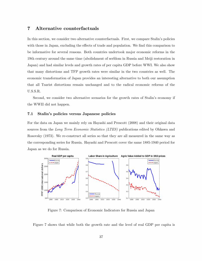
7 Alternative counterfactuals

In this section, we consider two alternative counterfactuals. First, we compare Stalin�s policies

with those in Japan, excluding the e¤ects of trade and population. We �nd this comparison to

be informative for several reasons. Both countries undertook major economic reforms in the

19th century around the same time (abolishment of serfdom in Russia and Meiji restoration in

Japan) and had similar levels and growth rates of per capita GDP before WWI. We also show

that many distortions and TFP growth rates were similar in the two countries as well. The

economic transformation of Japan provides an interesting alternative to both our assumption

that all Tsarist distortions remain unchanged and to the radical economic reforms of the

U.S.S.R.

Second, we consider two alternative scenarios for the growth rates of Stalin�s economy if

the WWII did not happen.

7.1 Stalin�s policies versus Japanese policies

For the data on Japan we mainly rely on Hayashi and Prescott (2008) and their original data

sources from the Long Term Economic Statistics (LTES) publications edited by Ohkawa and

Rosovsky (1973). We re-construct all series so that they are all measured in the same way as

the corresponding series for Russia. Hayashi and Prescott cover the same 1885-1940 period for

Japan as we do for Russia.

1890 1900 1910 1920 1930 1940500

1000

1500

2000

2500

3000

PP

P 1

990 

inte

rnat

iona

l dol

lars

Real GDP per capita

1890 1900 1910 1920 1930 19400.3

0.4

0.5

0.6

0.7

0.8

0.9Labor Share in Agriculture

1890 1900 1910 1920 1930 19400.1

0.2

0.3

0.4

0.5

0.6

Agric Value Added to GDP in 1913 prices

Russ iaJapan

Russ iaJapan

Russ iaJapan

Figure 7: Comparison of Economic Indicators for Russia and Japan

Figure 7 shows that while both the growth rate and the level of real GDP per capita is

37

1890 1900 1910 1920 1930 19400.8

1

1.2

1.4

1.6

1.8

2

AMRussiaJapan

1890 1900 1910 1920 1930 19400.5

1

1.5

2

2.5

AA

RussiaJapan

1890 1900 1910 1920 1930 1940­2

0

2

4

6

8

10

12

τCRussiaJapan

1890 1900 1910 1920 1930 19400

5

10

15

20

25

τWRussiaJapan

1890 1900 1910 1920 1930 19400

2

4

6

8

10

12

τRRussiaJapan

1890 1900 1910 1920 1930 1940­0.2

0

0.2

0.4

0.6

0.8

τK

RussiaJapan

Figure 8: Wedges and sectoral TFPs in Russia and Japan.

roughly the same in Russia and in Japan in 1885-1913, the structural composition of the two

economies is quite di¤erent. The fraction of labor force employed in non-agricultural sector

in Japan is signi�cantly smaller than in Russia and declines steadily throughout the sample

period. The role of agriculture in the economy is also much less important than in Russia, with

only about 25 percent of value added being produced in agriculture. A part of this di¤erence

can be explained by the international specialization whereas Japan imports agricultural goods.

After WWI Japan mostly follows its pre-war pattern of development, with some acceleration

in the GDP per capita growth rate after 1933. Finally, our analysis shows a big wedge �R

in Japan that falls over time. It is mainly driven by the value of residential farm structures.

According to the LTES, value of those structures to agricultural output is greater than the

value of all (residential and non-residential) agricultural capital stock to agricultural output in

Russia in 1885. Ideally, we would like to exclude residential structures from our measures of

capital but for Tsarist Russia we do not have necessary data.

We start by comparing the wedges for Russia, both under the Tsars and under Stalin, with

those in Japan. This comparison is presented in Figure 8. The tsarist economy and the economy

of Japan were quite similar before 1913. Russia lagged Japan in terms of manufacturing

38

1915 1920 1925 1930 1935 1940 1945 1950 1955 19601000

1500

2000

2500

3000

3500

4000

4500

5000

5500

PP

P 1

990

 inte

rna

tiona

l do

llars

Real GDP per capitaRussiaJapanRussia with Japanese wedgesTsarist Russia

Figure 9: Real GDP per capita in Russia, Japan and Russia with Japanese wedges

TFP in the 1890s but then by and large caught up in the �rst decade of 1900s. The average

manufacturing TFP growth for the pre-1913 period was 0.66 percent for Russia and 0.86 percent

for Japan. Russia and Japan had essentially equal agricultural TFP. The intersectoral capital

distortion was signi�cantly higher in Japan before 1913 but declined signi�cantly throughout

the period. The intersectoral labor distortion was lower in Japan �this likely re�ects the fact

that the institution of obschina in Russia was much more distortionary than the barriers for

labor mobility in Japan that Hayashi and Prescott (2008) focused on. There is no signi�cant

di¤erence in the pattern of the intertemporal wedge.

After WWI the path of Japanese wedges and TFP growth rates changes albeit less signi-

�cantly than it did in Soviet Russia. Most notably the TFP growth rate in non-agriculture,

and to a lesser extent agriculture, accelerates.

Our counterfactual exercise envisions the path of the Russian economy under the as-

sumption that after 1913 the speed of changes in the Tsarist economy would be similar to

those in Japan. In particular, for all wedges and TFP we constract new series for Rus-

sia using the law of motion �Russiat = �Russia1913�Japant

�Japan1913

for t = 1914; :::; 1940 where � t 2

f�C;t; �K;t; �W;t; �R;t; AM;t; AA;t; GM;tg : To control for Russia�s population and comparative

39

Gain from policy forPolicy [28-40] [28-1] [40-1] [40-1], K1940�K -4.5% 1.6% 6.4% 4.3%�C 3.2% 9.7% 9.4% 7.4%�W 3.5% 4.5% 12.4% 13.7%

GM and �R 4.6% 3.6% 2.9% 2.4%AM -17.4% -36.6% -53.1% -52.6%AA -12.9% -5.7% -0.1% 1.1%

ex and q - - - -Total -41.3% -31.0% -22.7% -24.2%

Total net of K1928 -23.4% -22.7% -22.2% -24.0%

Table 3: Welfare Decomposition: Stalin vs. Japan

advantage we keep the actual realizations of population growth and trade as occured in the

data. After 1940 we extrapolated the average growth rates of all wedges between 1928 and

1940.28

Figure 9 compares implied real GDP per capita (red line) with actual real GDP per capita

in Japan and U.S.S.R, as well as with our projection of real GDP in Soviet Russia and in

Tsarist Russia under the assumption of no changes in wedges. Before 1940 the constructed

path of Russia�s GDP per capita is very similar to that of Japan. The gap between projected

GDP per capita in Russia and USSR increases after 1940, mainly due to higher productivity

growth. Even though by construction these series do not take into account the drop in GDP

during the WWII these projections understate the eventual level of GDP achieved by Japan

after 1960.

Table 3 shows welfare decomposition for this economy. It is evident that imposing the

Japanese wedges substantially improves the Tsarist counterfactual simulation. The big wel-

fare gain comes from the improvements in productivity. While distortions in Stalin�s policies

decrease and are generally lower than those in Japan, lower productivity wipes out those gains

and leads to signi�cant welfare losses.

7.2 Alternative post-1940 growth scenarios

One projection for which long-term values are of particular interest are the growth rates of TFP

in the two sectors. Recall that the benchmark counterfactual assumed that the sectoral TFP28Since GM;t signi�cantly increased in Japan before WWII, we set GM;t = GM;1940 for t > 1940:

40

growth rates post-1940 for the Stalin�s economy are equal to those for the Tsarist economy.

We now provide a calculation for two additional alternative scenarios.

For our benchmark simulations for 1 we assumed that the TFP in agriculture and non-

agriculture in Soviet economy continues to grow with Tsarist trends after 1940. It is possible

to make plausible claims that this assumption either understates or overstates the productivity

growth in Soviet Russia had it not joined the WWII. On the one hand, actual productivity

growth in non-agriculture is signi�cantly lower in 1935-1940 than Tsarist trend. On the other

hand, one could argue that the low productivity is a temporary result of rapid reallocation and

adjustment costs and would have increased in the medium term. To address these concerns

we consider two scenarios.

The �rst scenario uses for the projection of the sectoral TFP growth under Stalin post

1940 the trend of the sectoral TFP growth in 1937-1940 (that is, the regression line drawn

through these values). This approach implies a continued decline in manufacturing TFP but a

speed-up in agricultural TFP growth. Table 15 in the online appendix shows that the adverse

e¤ect on manufacturing TFP far outweighs the favorable e¤ect on agricultural TFP. The net

e¤ect of this alternative path comes at an additional welfare cost of around -4.5 percent of

consumption for the generation born in 1928, and an additional cost of -7.8 percent for the

generation born in 1940.

The second scenario uses the realized levels of TFP and wedges under Stalin post WWII.

We use data produced by Moorsteen and Powell (1966) to compute estimates of all the wedges

for Stalin�s economy for the period 1945-195329 and compare it to our simulations. Figure 10

compares the actual realization of wedges after WWII to our projections. After a recovery

period from the WWII, the wedges in the Soviet economy stabilized around their pre-WWII

levels by 1950. The exception is TPF in manufacturing, which reaches higher levels than our

projections but is still below the Tsarist trend.

In the second scenario, we use average values of the wedges for the period 1950-1953

reported in Table 4 instead of the projected wedges for Stalin�s economy. We use levels of

sectoral TFP for 1953 to compute growth rates of TFP for the post-1940 period and use these

growth rates in the second alternative scenario.

29Stalin died in 1953 and signi�cant changes took place in the aftermath of his death. The study of thosereforms is outside of the scope of this paper.

41

1930 1935 1940 1945 195070

80

90

100

110

120

130

AM

1930 1935 1940 1945 1950150

200

250

300

350

AA

1930 1935 1940 1945 19500

5

10

15

20

25

τW and τR

1930 1935 1940 1945 19500

2

4

6

8

10

12

τC

1930 1935 1940 1945 1950

­0.2

­0.1

0

0.1

0.2

0.3

τK

1930 1935 1940 1945 19500

0.05

0.1

0.15

0.2

0.25

0.3

GM/YMBaselineTsarStalin

BaselineTsarStalin

τW

 Baseline

τR

 Baseline

τW

 Tsar

τR

 Tsar

Stalin

BaselineTsarStalin

BaselineTsarStalin

BaselineTsarStalin

Figure 10: Wedges and sectoral TFPs under Tsar and Stalin.

Table 17 in the online appendix reports the impacts of this alternative scenario on the

baseline welfare decomposition. We �nd that most of the wedges take values close enough to

our baseline simulation. As a result, their impact is minimal. The largest changes come from

faster TFP growth in the manufacturing sector, and higher prices scissors, which each produce

under 3 percent extra welfare gains in the long-run.

8 Robustness

We prepared an extensive online appendix that provides a comprehensive set of robustness

exercises. This appendix also contains the details of a variety of alternative assumptions already

mentioned in the paper. We now brie�y summarize the main implications of robustness.

First, we assess the sensitivity of our estimates of the wedges to measurement error in the

data by conducting a Monte-Carlo exercise as follows. We create arti�cial data series by adding

1 percent log-normal random disturbances to the original data series. We use this arti�cial

data to compute pseudo-series for the wedges. Using 1000 such pseudo-series for the wedges

we compute percent standard deviations of the pseudo-wedges for the whole period and for

42

sub-periods. The elasticities of the wedges with respect to measurement error are computed

as the ratios of the percentage standard deviations of the pseudo-wedges to the percentage

measurement errors. We �nd that 1 percent measurement error arti�cially introduced into the

data leads on average to 1-5 percent changes in the values of the wedges. We then proceed

with �nding the standard errors for the decomposition of the welfare (Table 1).

We �nd that the standard errors are relatively low, as even two standard deviations, in

most cases, do not signi�cantly alter our main conclusions. The same is true for the standard

errors in the paths of the manufacturing labor share, total capital and total GDP in 1913

prices achieved by Stalin�s policies compared to the potential path coming from a continuation

of Tsarist policies.

Second, we provide a sensitivity analysis with respect to calibrated parameters. In each

exercise one of the parameters f�A;K ; �A;N ; �M;K ; �M;N ; ; �g is changed. For each alternative

calibration new time series for wedges are recovered from the data. These new wedges are used

to evaluate the welfare gains of policies and the e¤ects on key variables. Most of these e¤ects

are small. The largest change comes from varying the subsistence level A. However, even a

10 percent decrease in subsistence leaves the signs and the magnitudes of most of our results

intact, while a 10 percent increase would only reinforce our conclusions.

Third, we provide a sensitivity analysis with respect to projections of the wedges into the

future. In each exercise one of the projected long-term values for the wedges is changed to

its alternative value reported. Each alternative wedge value is used to evaluate welfare gains

of policies and the e¤ects on key variables coming from alternative assumptions about future

fundamentals. Speci�cally, we proceed as follows. We �rst report an e¤ect of a 1 percent

change in a fundamental. If we believed that the data has a 2 percent std measurement error,

and that each 1 percent change in a wedge translated into 2-3 percent std of the wedge, then we

multiply all numbers in the 1 percent change calculation by a factor coming from the impact

of this 2-3 percent std change. This would give us an approximate standard deviation of the

con�dence bounds on our main estimates due to potential measurement errors in the data. We

�nd that these con�dence bounds are quite narrow.

43

9 Conclusion

We started this paper with a question: "Was Stalin necessary?". Tsarist economy, even in

our conservative version assuming that it would not experience any decline in frictions, would

have achieved a rather similar structure of the economy and the levels of production as Stalin�s

economy. However, this structural transformation would be achieved at a signi�cant cost

in terms of economic welfare measured in consumption equivalents. The short-run (1928-

1940) costs of Stalin�s policies are very signi�cant for an economy in a peaceful period. Our

comparison with Japan leads to astonishingly larger welfare costs of Stalin�s policies.

Our projections post 1940 are more speculative. Our conservative benchmark estimates

(giving perhaps undue credit to Stalin�s TFP projections) point to a long-term welfare gain

coming from the reduction of the frictions that outweigh the lackluster performance of TFP.

10 References

Acemoglu, Daron, and James A. Robinson (2012) Why nations fail: The Origins of

Power, Prosperity, and Poverty. Crown Business

Allen, Robert C (1997) "Agricultural marketing and the possibilities for industrializa-

tion in the Soviet Union in the 1930s", Explorations in Economic History, Volume 34, Issue 4,

October 1997, pp. 387-410.

Allen, Robert C (2003) Farm to factory : a reinterpretation of the Soviet industrial

revolution, Princeton University Press.

Barsov, A. (1969) Balans stoimostnykh obmenov mezhdu gorodom i derevnei. Moscow:

Nauka. [in Russian]

Bergson, Abram (1961) The real national income of Soviet Russia since 1928. Harvard

University Press.

Buera, F. J., and Kaboski, J. P. (2009). "Can traditional theories of structural change

�t the data?" Journal of the European Economic Association, 7(2-3), pp. 469-477.

Caselli, F., and Coleman,Wilbur John II. (2001). "The U.S. structural transforma-

tion and regional convergence: A reinterpretation". Journal of Political Economy, 109(3), pp.

584-616.

Chari, V. V., Kehoe, P. J., and McGrattan, E. R. (2007). "Business cycle account-

44

ing". Econometrica, 75(3), pp. 781-836.

Cole, H. L., and Ohanian, L. E. (2004). "New deal policies and the persistence of the

great depression: A general equilibrium analysis". Journal of Political Economy, 112(4), pp.

779-816.

Conquest, Robert (1986) The harvest of sorrow: Soviet collectivization and the terror-

famine. New York : Oxford University Press.

Chernina, Eugenia, Dower, Paul Castaneda and Markevich, Andrei (2011)

�Property Rights and Internal Migration: The Case of the Stolypin Agrarian Reform in the

Russian Empire.�Mimeo, New Economic School. Available at SSRN: http://ssrn.com/abstract=1730730

Crisp, Olga (1978) "Labor and Industrialization in Russia" Cambridge Economic History

of Europe, vol 7, pt 2. Cambridge University Press.

Davies, R.W (1990) From tsarism to to the New Economic Policy. Macmillan Academic

and Professional Ltd.

Davies, R.W., Mark Harrison and S.G. Wheatcroft (1994) The Economic trans-

formation of the Soviet Union, 1913-1945 ; New York : Cambridge University Press.

Davies, R.W (1998) Soviet economic development from Lenin to Khruschev, Cambridge

University Press.

Davies, R.W., and S.G. Wheatcroft (2004) The years of hunger: Soviet agriculture,

1931-1933 Palgrave Macmillan.

Ellman, Michael (1975) �Did the Agricultural Surplus Provide the Resources for the

Increase in Investment in the USSR During the First Five Year Plan?�Economic Journal, Vol.

85, No. 340, pp. 844-863.

Feldman, Michael (1928) �K Teorii Tempov Narodnogo Dokhoda� Planovoe Khozi-

aistvo, No. 11, pp. 146-170 and No. 12 pp. 157-178. [in Russian]

Gerschenkron, Alexander (1947) �The Soviet indices of industrial production.�Review

of Economics and Statistics, 29, 217-26.

Gerschenkron, Alexander (1962) Economic backwardness in historical perspective Har-

vard University Press.

Gregory, Paul (1982) Russian national income, 1885-1913, Cambridge University Press.

Gregory, Paul, and Mark Harrison (2005). �Allocation under Dictatorship: Research

in Stalin�s Archives.�Journal of Economic Literature, 43(3), pp. 721-761.

45

Hayashi, F., & Prescott, E. C. (2008). "The depressing e¤ect of agricultural institu-

tions on the prewar japanese economy". Journal of Political Economy, 116(4), pp. 573-632.

Herrendorf, B., Rogerson, R., and Valentinyi, A. (2009). "Two perspectives on

preferences and structural transformation" NBER Working Paper 15416.

Jacks, David S. (2005). "Intra- and International Commodity Market Integration in

the Atlantic Economy, 1800-1913.", Explorations in Economic History, 42(3), pp. 381-413.

Jasny, Naum (1951). "Labor and Output in Soviet Concentration Camps", Journal of

Political Economy, vol. 59, pp. 405-19.

Kahan, A. (1967) "Government Policies and the Industrialization of Russia", Journal of

Economic History, 27, pp. 460-77.

Khanin, G. I. (1988) "Ekonomicheskij rost: al�ternativnaya otsenka", Kommunist, 17.

[In Russian]

Khlevnyuk, Oleg (2009) Master of the house: Stalin and his inner circle, Yale University

Press.

Markevich, Andrei and Mark Harrison (2011a) "Great War, Civil War, and Recov-

ery: Russia�s National Income, 1913 to 1928," Journal of Economic History 71:3, pp. 672-703.

Markevich, Andrei and Mark Harrison (2011b) "Russia�s National Income: Ap-

pendix" Online appendix.

Millar, James (1974). �Mass Collectivization and the Contribution of Soviet Agriculture

to the First Five-Year Plan: A Review Article.�Slavic Review, Vol. 33, No. 4, pp. 750-766.

Moorsteen, Richard H. and Raymond P. Powell (1966) The Soviet capital stock,

1928-1962, Homewood, Ill., R. D. Irwin.

Murphy, Kevin M., Andrei Shleifer and Robert W. Vishny (1989) Industrializa-

tion and the Big Push Journal of Political Economy, Vol. 97, No. 5, pp. 1003-1026.

Nove, Alec (1962) "Was Stalin Really Necessary?" In his Was Stalin Really Necessary?

London: George Allen & Unwin Ltd 1964, pp. 17-39.

Nove, Alec (1992) An Economic History of USSR 1917-1991, Third Edition, 1992,

Penguin.

Preobrazhensky, Evgeny (1965) The New Economics. Oxford: Clarendon Press.

Rosenstein-Rodan, P.N. (1943) �Problems of Industrialization of Eastern and South-

eastern Europe.�Economic Journal, , 53, pp. 202-11.

46

Sah, Raaj Kumar and Joseph Stiglitz (1984). �The Economics of Price Scissors.�

American Economic Review, Vol. 74, No. 1, pp. 125-138.

Seton, F. (1959) "Production functions in Soviet industries", American Economic Re-

view, XLIX.

Stokey, N. L. (2001). "A quantitative model of the british industrial revolution, 1780-

1850". Carnegie-Rochester Conference Series on Public Policy, 55, pp. 55-109.

Von Laue, T.H. (1963) Why Lenin? Why Stalin? A Reapprisal of Russian Revolution,

1900-30 (London).

47

11 Appendix A: Construction of data

11.1 Capital stock

11.1.1 Russia 1885-1913

For Russia in 1885-1913 all data is from Gregory (1982) and it is computed in 1913 prices.

Capital in agriculture is a sum of value of livestock (table H.1), accumulated agricultural

equipment (table I.1) and net capital �xed capital stock in agriculture (table J.1). Agricultural

structures include rural residential structures and Gregory does not provide a separate estimate

of those. Gregory provides estimates of livestock and net capital stock, but gives investment in

agricultural equipment. We derive the stock of agricultural equipment with perpetual inventory

method by assuming a 5 percent depreciation.

Capital stock in non-agriculture is de�ned as the value of accumulated industrial equipment

(table I.1), net stock of industrial structures (table J.1), industry inventories (table K.1),

railroads (table L.1). The values for the stock of structures, inventory, railroads and urban

housing are taken directly from Gregory, while the stock of accumulated industrial equipment

is obtained by perpetual inventory method assuming a 5 percent depreciation.

This de�nition of capital stock includes rural residential housing into agricultural capital

stock but does not include urban residential housing in any measure of capital stock. The

reason for this is as follows. Ideally, following Hayashi and Prescott (2008) we would like to

exclude housing stock from all measures of capital. Gregory does not provide a breakdown

of rural capital between residential and nonresidential. We do not include urban residential

housing into non-agricultural capital stock since the estimates of urban capital stock di¤er

dramatically for pre 1913 and post 1928 Russia, which we view as unrealistic.

Total capital stock is de�ned as a sum of capital stock in agriculture and non-agriculture.

We computed investments in each sector from the series of capital stocks assuming a 5

percent depreciation.

11.1.2 Russia 1928-1940

For Russia in 1928-1940 we use data from Moorsteen and Powell (1966). All data is in 1937

prices.

We use the data on the composition of gross residential �xed capital stock (table 3-3) to

48

�nd the fraction of urban residential capital stock in gross residential �xed capital stock. We

assumed that the same ratio holds for net residential capital stock (table T-15) to �nd the

value of net urban residential capital stock.

We de�ne non-agricultural capital stock as net nonresidential, nonagricultural capital stock

(table T-25). This de�nition includes industrial �xed structures, equipment and inventories.

We de�ne agricultural capital stock as net �xed capital stock minus net nonresidential

nonagricultural capital stock and minus the value of urban residential housing.

Total capital stock is de�ned as a sum of capital stock in agriculture and non-agriculture.

11.2 Exports and international prices

The data for total volume of exports and imports for tsarist Russia is from Gregory (1982),

Table M-1. We use the data from Davies (1990), Table 56, to �nd composition of exports and

imports for 1913. We assume that the same composition holds for 1885-1913 and compute net

exports of agricultural goods and net imports of non-agriculture goods.

The data for volume of exports and imports for the USSR from 1928 to 1938 is from Davies

et al (1993). The provide index of exports and imports relative to 1913 and we use the numbers

for 1913 trade from Gregory (1982) to obtain volume of trade in 1913 prices. We impute the

values for 1939 and 1940 by assuming that the remain at the 1938 level. We use the data from

Davies (1990), Table 58, to �nd composition of exports and imports for 1927/1928. We assume

that the same composition holds for 1928-1940 and compute net exports of agricultural goods

and net imports of non-agricultural goods.

We use data on Soviet terms of trade from Davies et al (1993), table 50. Unfortunately we

found no comparable numbers for tsarist period.

As a proxy for the international prices of Russian exports we take New York state price of

wheat. The dollar prices for wheat are from Jacks (2005). The nominal prices de�ated by the

US CPI are from the NBER Macrohistory Database.

11.3 Output, consumption and investment by sector

11.3.1 Russia 1885-1913

We computed investments in each sector from the series of capital stocks assuming a 5 percent

depreciation. We computed GNP from NNP series in Gregory (1982), Table 3.1 by adding a 5

49

percent depreciation to the total capital stock.

We did not �nd reliable data for value added in manufacturing and agriculture for all years.

Gregory (1982) in Table 3.6 reports that in 1913 50.7 percent of value added is produced in

agriculture. He also provides numbers for retained consumption of agricultural goods which

were not marketed by the peasants (Table M.1) for all time period. We assume that fraction

of value added of agricultural production to the retained consumption is at the same level as

in 1913 to obtain the estimate of the value added in agriculture during 1885-1913. The value

added in manufacturing is obtained by subtracting the value added in agriculture from GNP.

Gregory reports breakdown of imperial and local government expenditures for selected years

(Tables F.4 and G.4). For the benchmark analysis we took defence expenditures as our measure

of government sector and we checked the robustness of our conclusion by added administrative

expenditures. The data for the missing years was obtained by linear interpolation.

To obtain relative prices, we computed nominal value added of agriculture following the

same steps as we did for the value added in agriculture in 1913 prices. The ratio of the two

gives us a price de�ator for agriculture. Gregory in Tables 3.1 and 3.2 reports net investments

in current prices and 1913 prices, which allow us to compute investment price de�ator and

depreciation in current prices. Using Gregory�s estimates of National income in current prices

and our estimates of depreciation in current prices we obtain GNP in current prices. By

subtract value of agriculture in current prices we obtain the value of manufacturing in current

prices and price de�ator for manufacturing goods. The ratio of the price de�ator for agricultural

goods to the price de�ator of manufacturing goods yields relative price of agricultural goods.

11.3.2 Russia 1928-1940

Moorsteen and Powell (1966), Table P.1 provide estimates of GNP and production by sector in

1937 prices. We measure agricultural sector as total output in agriculture, and manufacturing

as GNP minus agricultural sector.

Moorsteen and Powell also provide a breakdown of government expenditures in the same

table. For the benchmark analysis we took defence expenditures as our measure of government

sector and we checked the robustness of our conclusion by added administrative expenditures.

Finding appropriate series for relative prices is particularly challenging. Many o¢ cial prices

are not allocative and they do not necessarily re�ect the shadow prices and costs that economic

50

agents face. We rely on the work of Allen (1997) who constructs transaction prices (Table A2)

which he argues are the best measure of the prices that peasant faced. These prices are

constructed as a ratio of free retail non-food prices to wholesale agricultural prices.

11.4 Population and labor force

11.4.1 Russia 1885-1913

The data for population is from Gregory (1982), Table 3.1. He reports of the data for the

territory of Russian empire excluding Finland and we follow his convention.

We obtain composition of labor force from Davies (1990) and Gregory�s estimates. Davies

(1990), Table 3 provides estimate of the composition of labor force by sector in 1913. Gregory

(1982), Table 6.3 reports growth rates for labor force by sector in for di¤erent time periods

during 1885-1913. We use these growth rates to backtrack labor force for years before 1913.

11.4.2 Russia 1928-1940

It is di¢ cult to obtain reliable data for the composition of labor force. There have been

three censuses in Russia, in 1926, 1937 and 1939, but the results of the 1937 are mostly

unpublished and many historians question reliability of 1939 census. There are o¢ cial numbers

for employment in various non-agricultural sectors of the economy for select years (Davies et al

(1994), table 12). Comparing to the Census data, they do not cover all of the non-agricultural

labor force, but give reasonably good approximation of the growth rate of the non-agricultural

labor force over the entire time period. According to the census data, non-agricultural labor

force increased by a factor 3.37 between 1926 and 1939, while o¢ cial survey numbers show an

increase of 3.19 between 1928 and 1940. We try to use a procedure that follows our estimate

of tsarist labor force as closely as possible.

We use population numbers from Davies et al (1994), Table 1. From 1926 census (Davies

et al (1994), Table 11) we obtain composition of labor force by sector. We assume that each

sector covered by the survey data growths at the same rate as implied by the surveys. This

gives us an estimate of non-agricultural labor force for each year. The implied increase in the

labor force is 3.36, which closely matches the implied growth of non-agricultural labor force

from 1939 census. To �nd agricultural labor force we assume that labor force participation in

all years is the same as in 1926, and �nd agricultural labor force as a residual.

51

This procedure implicitly assumes that fraction of labor force to population did not change

between 1926 and 1939. This assumption approximately holds in the data. Ratio of labor

force to population is 49 percent in 1926 and 50 percent in 1939.

11.5 Adjustment for border changes, conversion prices

Using procedure above we obtained two data sets, one for Russia in 1885-1913 in 1913 borders

(excluding Finland) and 1913 prices and the other on for the USSR in 1928-1940 in pre-1940

borders and 1937 prices. In this section we discuss conversion of all prices and quantities to

have comparable units.

The territory of Russian empire excluding Finland is 21,474 sq km, while the territory of

the USSR in pre-1940 borders is 21,242 sq km (Markevich and Harrison (2011), Table 2). Thus

the areas of the two territories are quite similar and therefore we assume that land endowments

are the same in the two periods and do not make any border adjustments.30

Markevich and Harrison (2011) also report that NNP in 1913 prices in Russia decreased

from 20,266 mln rubles to somewhere between 15,600 and 17,600 mln rubles in 1928. We take

the average of the two numbers and assume that NNP in Russia in 1928 is 16,600 mln rubles in

1913 prices. Markevich and Harrison (2011b) report (Table A10) that fraction of agriculture in

NNP in Russian Empire excluding Finland was 44.3 percent in 1913 (50.9 percent if forestry,

�shing and hunting is included in de�nition of agriculture) and in USSR interwar borders

was 44.4 percent (50.8 percent with forestry, �shing and hunting). Therefore we assume that

fraction of agriculture in GDP is the same in 1913 and 1928. Since all these numbers are given

in 1913 prices, they imply that quantities of agricultural and nonagricultural goods decreased

proportional to the decrease in the NNP. This gives us a relationship

pA1913YA1913

Y A1928Y A1913

= pA1913YA1928 =

pA1913pA1937

pA1937YA1928;

which implies thatpA1937pA1913

=pA1937Y

A1928

pA1913YA1913

20; 266

16; 600:

We �nd pM1937=pA1913 analogously.

30While land endowment remained the same, Russian empire lost richer territories (Finland, Poland, WesternBelarus and Ukraine, Causasus) and gained poorer territories in Central Asia. Tsarist NNP in 1913 measured inUSSR interwar boarders would decrease from 22 mln rbl to 16.5 mln rbl (Markevich and Harrison (2011), Table1). In the context of our model this di¤erences will be re�ected in TFPs and therefore we do not recomputetsarist output in Soviet borders.

52

12 Appendix:Tables

Table 4 shows a variety of values which the wedges take for di¤erent periods and in di¤erent

scenarios. The �rst three columns of Table 4 show the average values of the wedges measured for

three subperiods: 1885-1913, 1928-1936 and 1937-1940. The next two columns show projected

values for the wedges used in the two baseline counterfactual simulations: for Stalin and for

Tsar. Columns "Japan" and "50-53" show the average values for the wedges inferred from

Japanese data for the period 1914-1940 and for the USSR after World War II for the period

1950-1953.

Table 5 is the analogue of Table 2 in the main body of the paper. We measure the e¤ect

of di¤erent wedges on the behavior of the variables. The third column of the table is exactly

the �rst column of Table 2.

Period Average ProjectionWedge [85-13] [28-36] [37-40] Stalin Tsar Japan [50-53]Nt 1.0 0.78 0.78 0.78 1.0 � ��K 0.085 0.066 0.038 0.038 0.085 0.070 0.045�C 0.24 3.19 0.52 0.52 0.24 0.13 0.89�W 5.66 13.11 4.71 4.71 5.66 4.35 4.61�R 1.75 6.18 1.76 1.76 1.75 2.75 1.29

(1 + �W )=(1 + �C) 5.89 4.76 3.80 3.80 5.89 4.85 3.02(1 + �R)=(1 + �C) 2.41 2.34 1.83 1.83 2.41 3.50 1.22

GM 0.067 0.024 0.085 0.085 0.067 0.08 0.090AM 1.0 0.97 0.91 0.90 1.0 1.07 0.94AA 1.0 0.79 0.95 0.995 1.0 1.05 1.01

AM growth 0.66% -2.95% -1.12% 0.61% 0.61% 0.70% 1.23%AA growth 1.45% 0.35% 3.05% 0.97% 0.97% 1.21% 0.70%

ex 0.096 0.058 0.027 0.027 0.096 � 0.033q 0.66 1.07 1.58 1.58 0.66 � 1.65

Table 4: Average and Projected Wedges

53

Labor Share Capital OutputPolicy 28-36 37-40 1945 28-36 37-40 1945 28-36 37-40 1945�K 1.2% 4.2% 2.7% 3.7% 26.6% 37.0% 2.3% 11.6% 13.7%�C % 16.1% 1.7% 3.1% 24.0% 38.8% 14.0% 32.2% 12.3% 8.3%�W -14.2% 5.1% 4.0% -46.9% -29.1% -0.0% -36.0% -0.9% 4.8%GM and �R 2.2% 0.2% 0.3% 14.5% 10.0% 3.1% 5.2% 3.2% 1.3%AM 0.3% -0.4% -0.4% 3.0% -14.2% -15.8% -3.3% -11.2% -12.2%AA -5.9% -0.8% 0.2% -11.4% -14.1% -4.6% -20.7% -6.4% -1.2%ex and q 1.5% 2.8% 2.6% 3.2% 2.6% 3.5% 3.7% 4.1% 4.2%Total 2.8% 13.2% 12.6% -49.3% 15.3% 36.2% -23.9% 11.5% 18.7%

Table 5: E¤ects on Labor Share, Capital and real GDP

54