water chemistry data for selected springs, geysers, … · exception of intermediate sulfur redox...

Water Chemistry Data for Selected Springs, Geysers,

and Streams in Yellowstone National Park, Wyoming,

Beginning 2009 – Methods and Quality Assurance and

Quality Control

By R. Blaine McCleskey, Randall B. Chiu, D. Kirk Nordstrom, Kate M. Campbell, David A. Roth, James W.

Ball, and Terry I. Plowman

Both photographs are of Cistern Spring, Norris Geyser Basin, Yellowstone National Park. The photograph on the left is taken on

9/11/2009 and the photograph on the right is taken on 8/7/2013 about 1 week after Steamboat Geyser erupted causing Cistern

Spring to completely drain.

Suggested citation:

McCleskey, R.B., Chiu, R.B., Nordstrom, D.K., Campbell, K.M., Roth, D.A., Ball, J.W., and Plowman, T.I., 2014, Water-Chemistry Data for

Selected Springs, Geysers, and Streams in Yellowstone National Park, Wyoming, Beginning 2009: doi:10.5066/F7M043FS.

Any use of trade, product, or firm names is for descriptive purposes only and does not imply endorsement by the U.S. Government.

ii

Contents

Methods .................................................................................................................................................................... 1

Collection and Preservation of Water Samples .................................................................................................... 1

Field and Laboratory Measurements.................................................................................................................... 4

Field Measurements ......................................................................................................................................... 4

Laboratory Methods ......................................................................................................................................... 7

Major Cation and Trace Metal Determinations ............................................................................................ 11

Anion and Alkalinity Determinations ........................................................................................................... 12

Arsenic Redox Determinations ................................................................................................................... 13

Iron Redox Determinations ......................................................................................................................... 15

Ammonium Determinations ......................................................................................................................... 15

Mercury Determinations .............................................................................................................................. 16

Dissolved Organic Carbon .......................................................................................................................... 16

Water Isotope Determinations .................................................................................................................... 16

Acidity Determinations ................................................................................................................................ 17

Revised pH Measurements ......................................................................................................................... 19

Quality Assurance and Quality Control .................................................................................................................... 22

References Cited..................................................................................................................................................... 36

Figures

Figure 1. Percent difference between field and lab electrical conductivity using (A) the ISO-7888 temperature

compensation factor (ISO-7888, 1985) and (B) the McCleskey (2013) temperature compensation

factor .................................................................................................................................................... 6

Figure 2. Flow-chart for the analytical technique used for the final selection of element-specific data. ............. 12

iii

Figure 3. As(T) concentrations determined by HGAAS in the FA-HCl split plotted against As(T) concentrations

determined by ICP-OES in the FA-HNO3 split. .................................................................................. 14

Figure 4. The percent differences in the measured As concentrations plotted against H2S concentrations. ..... 15

Figure 5. Flow chart illustrating the process for refining the acidity pH value. ................................................... 19

Figure 6. Flow chart showing the pH selection process. (C.I., charge imbalance) ............................................ 21

Figure 7. Frequency distribution of charge imbalance for samples having major cation and anion

determinations. ................................................................................................................................... 23

Figure 8. Electrical conductivity imbalance compared with charge imbalance. ................................................. 23

Figure 9. Cation and trace metals concentrations determined by ICP-MS and ICP-OES plotted on a linear (A)

and log10 (B) scale. ............................................................................................................................ 26

Figure 10. Total dissolved iron determined by ICP-OES and FerroZine for all data (A) and for iron concentrations

less than 5 mg/L (B). .......................................................................................................................... 27

Tables

Table 1. Sample split and preservative, constituents, and sample treatment…..………………………………….3

Table 2. Analytical techniques, detection limits, equipment used, and analytical method references……….….8

Table 3. Analytical Measured concentrations in standard reference water samples…………………………….28

1

Methods

Collection and Preservation of Water Samples

Water samples from hot springs, geysers, and pools were collected as close to the discharge

source as possible. For streams, tributaries, and overflow drainage channels, water samples were

collected as close to the center of flow as possible and in areas that appeared to be well mixed. Extreme

care was taken to safely collect water samples from the geothermal sites, to protect fragile hot-spring

mineral formations, and to minimize changes in temperature, pH, and water chemistry during sampling.

Samples were collected from the middle of large springs, pools, and geysers by positioning the sample

tubing intake using an insulated stainless-steel container as a flotation device attached to the end of an

extendable aluminum pole. At more easily accessible sites, the tubing intake was positioned in the

source or channel by hand. A Teflon block attached to the end of the sampling tubing was used as a

weight to keep the sample tubing in place.

Samples were collected and filtered on site by one of three techniques. The first technique, used

for most samples, consisted of pumping water directly from the source with a battery-operated

peristaltic pump fitted with silicone tubing through a pre-cleaned 142-millimeter (mm) diameter all-

plastic filter holder (Kennedy and others, 1976) containing a 0.1-micrometer (µm) pore size mixed-

cellulose-ester filter membrane. The second technique, which was used for samples collected from

Upper Geyser Basin in 2009, consisted of filling a 1-L bottle with source water and within an hour

filtering the sample by filling a 60-milliliter (mL) syringe with sample water, rinsing three times, and

immediately forcing the water through a 25-mm disposable filter having a mixed-cellulose-ester

membrane with a pore size of 0.2 µm. These two techniques were used by USGS scientists and have

sample numbers with coding yyWA### (where yy is the last 2 digits of the year and ### is a 3 digit

2

number). High-frequency samples collected by collaborators (sample numbers with coding Y10G###)

were filtered through disposable 0.45-µm capsule filters (Geotech Environmental Equipment, Inc.).

As many as 12 sample bottles were filled at each site. Sequential aliquots were filtered into

separate containers for the determination of inorganic constituents, redox species (iron, arsenic, and

sulfur), stable hydrogen and oxygen isotopes of water, and dissolved organic carbon (DOC). Container

preparation, storage, and stabilization methods for filtered samples are summarized in table 1. With the

exception of intermediate sulfur redox species and silica aliquots, the sample bottles were rinsed with

filtered water, the samples were then collected, and then stabilizing reagents, if needed, were added.

Stabilizing reagents for intermediate sulfur species were put into the sample bottles before the samples

were collected, and the silica aliquot was diluted on site with deionized water; therefore, these bottles

were not pre-rinsed.

Dissolved sulfide in each sample was preserved with an equal volume of sulfide anti-oxidant

buffer (SAOB, 0.2M disodium EDTA, 2M sodium hydroxide, 0.19M acorbic acid; Thermo Fisher

Orion). To prevent over-estimation of thiosulfate (S2O3) and polythionate concentrations by dissolved

sulfide, S(-II) oxidation was minimized by adding zinc acetate (Zn(COOCH3)2) to the sample bottles

before the samples were collected. This technique precipitates S(-II) as zinc sulfide (ZnS). The ZnS in

the samples was further stabilized by adding NaOH. Polythionate was converted to thiocyanate (SCN)

by adding potassium cyanide (KCN) to that sample split (Moses and others, 1984). For the analysis of

dissolved SiO2 in thermal waters, 0.5 mL of sample was diluted on site to 25 mL (by volume: 2009-

2012 and by mass beginning in 2013) with deionized water to minimize precipitation of SiO2 as the

sample cooled in the field.

Samples for the determination of DOC were filtered and collected in a glass bottle that had been

baked at 600°C. At least 1 liter (L) of sample water was passed through the all-plastic plate-filter

3

assembly before a DOC sample was collected. With the exception of the cation, water isotope, and silica

dilution samples, all sample aliquots were chilled as soon as practical after sample collection.

Table 1. Sample split and preservative, constituents, and sample treatment.

[DOC, dissolved organic carbon; H2SO4, sulfuric acid; HNO3, nitric acid; K2Cr2O7, potassium dichromate; v/v, volume per

volume; °C degrees Celsius]

Constituent(s) to be determined Storage container and preparationStabilization treatment in addition to filtratation

and refrigeration

Major anions (Br, Cl, F, and SO4), alkalinity as HCO3,

acidity, density, and nitrate (NO3)

Clear polyethylene bottles (250-mL), soaked in

deionized water and rinsed 3 times with deionized

water

None

Major cations (Ca, Mg, Na, K) and trace metals (As, Sb,

Ba, Be, Bi, B, Cd, Ce, Cs, Cr, Co, Cu, Dy, Er, Eu, Gd,

Ho, La, Pb, Li, Lu, Mn, Mo, Nd, Ni, Pr, Re, Rb, Sm, Se,

Sr, Te, Tb, Tl, Th, Tm, Sn, W, U, V, Yb, Y, Zn, and Zr)

Clear polyethylene bottles (125-mL), soaked in

5% HCl and rinsed 3 times with deionized water1% (v/v) concentrated redistilled HNO3 added;

samples were not chilled

Iron, arsenic, and antimony redox species (Fe(T), Fe(II),

As(T), As(III), Sb(T), and Sb(III))

Opaque polyethylene bottles (125-mL), soaked in

5% HCl and rinsed 3 times with deionized water

1% (v/v) redistilled 6 M HCl added

Arsenic redox species (As(T) and As(III)) Opaque polyethylene bottles (60-mL), soaked in

5% HCl and rinsed 3 times with deionized water

None

Ammonium (NH4) Clear polyethylene bottles (30-mL), soaked in 5%

HCl and rinsed 3 times with deionized water1% (v/v) 4 M H2SO4 added

Total mercury (Hg(T)) Borosilicate glass bottles (125-mL), soaked with

5% HNO3 and rinsed 3 times with deionized water

4% (v/v) Hg preservative (concentrated redistilled

HNO3 with 1 g/L K2Cr2O7) added

Silica (SiO2) Clear polyethylene bottles (30-mL), soaked in 5%

HCl and rinsed 3 times with deionized water

0.5 mL sample diluted to 25 mL with distilled water

on–site; samples were not chilled

Thiosulfate (S2O3) Clear polyethylene bottles (30-mL) rinsed 3 times

with deionized water1.7% (v/v) 0.6 M Zn(COOCH3)2 and 1% (v/v) 1 M

NaOH added

Polythionate (SnO6) Clear polyethylene bottles (30-mL) rinsed 3 times

with deionized water1.7% (v/v) 0.6 M Zn(COOCH3)2, 1% (v/v) 1 M NaOH,

and 1.7% (v/v) 1 M KCN

Dissolved organic carbon (DOC) Amber glass bottles (60-mL) baked at 600°C None

Water Isotopes (dD and d18O) Borosilicate glass bottles (60-mL) None; samples were not chilled

Sulfide (H2S) Clear polyethylene bottles (30-mL) 15 mL sulfide anti-oxidant buffer followed by 15 mL

sample

4

Field and Laboratory Measurements

Field Measurements

Measurements of temperature, pH, EMF (used to determine Eh), electrical conductivity, and

dissolved oxygen (DO, selected samples) were performed on site. Measurements of EMF and pH were

made on unfiltered sample water pumped from the source through an acrylic plastic flow-through cell or

directly in the spring, if safe. The flow-through cell contained a combination redox electrode, a

combination pH electrode, a thermistor, and test tubes containing buffer solutions for pH calibration. All

components were thermally equilibrated with the sample water before obtaining measurements. Where

practical, electrical conductivity and source temperature were measured by immersing the combined

conductance/temperature probe directly into the source as close to the sampling point as possible.

Otherwise, the probe was immersed in the flow-through cell. Because sample temperatures usually were

greater than the upper limit (45°C) of the DO probe, DO was determined using the azide modification of

the Winkler titration on selected samples (APHA, American Public Health Association, 1971).

Because field measurement of pH in geothermal waters is challenging and accurate pH

measurements are critical for interpreting analytical results (Ball and others, 2006), special care was

taken when measuring this parameter. At each site, the flow-through cell, temperature probe, electrode,

and calibration buffers were thermally equilibrated prior to calibration and measurement. The system

was calibrated using at least two bracketing standard buffers (chosen from among 1.68, 4.01, 7.00, or

10.00) using their pH values at the sample temperature (Midgley and Torrance, 1991). After calibration,

the pH electrode was placed in the sample water in the flow-through cell and monitored until no

changes in temperature (± 0.1°C) or pH (± 0.01 standard unit) were detected for at least 30 seconds.

Following sample measurement, the electrode was immersed in the standard buffer of pH closest to that

of the sample and allowed to equilibrate. The entire calibration and measurement process was repeated

5

as many times as necessary until the measured value for the buffer differed by no more than 0.05

standard units from its certified pH at the measured temperature.

Electrical conductivity measurements are typically referenced to 25°C using standard

temperature compensation factors (α). However, typical electrical conductivity compensation for acid

geothermal waters can result in large errors (>50%) because the hydrogen ion transport number (which

is not accounted for with the commonly used α’s) can be substantial and the temperature is often much

greater than 25°C. Figure 1 shows the percent difference between field and lab conductivity

measurements using the standard ISO-7888 temperature compensation factor (ISO-7888, 1985) that is

utilized by many conductivity meters and the McCleskey (2013) temperature compensation factor. The

method for electrical conductivity temperature compensation by McCleskey (2013) is more reliable for

calculating the electrical conductivity at 25°C for geothermal waters.

6

0 2 4 6 8 10-60

-50

-40

-30

-20

-10

0

10

20

30

0 2 4 6 8 10-60

-50

-40

-30

-20

-10

0

10

20

30

<40°C

40-60°C

60-80°C

>80°C

PE

RC

EN

T D

IFF

ER

EN

CE

pH

A.

B.

<40°C

40-60°C

60-80°C

>80°C

PE

RC

EN

T D

IFF

ER

EN

CE

pH

Figure 1. Percent difference between field and lab electrical conductivity using (A) the ISO-7888 temperature

compensation factor (ISO-7888, 1985) and (B) the McCleskey (2013) temperature compensation factor. The

dashed lines are ±10% for reference.

A mobile laboratory truck containing an ion chromatograph, ultraviolet-visible

spectrophotometer, autotitrator, and reagent-grade water purification system was set up so that unstable

intermediate sulfur oxyanion species could be determined as soon as possible after sample collection.

Iron redox species also were determined in the mobile laboratory. The autotitrator was used each

7

evening to perform alkalinity and acidity titrations before oxidation and hydrolysis reactions occurred,

and to determine H2S concentrations in samples preserved on site. Sulfide concentrations were

determined within 24 hours by ion-specific electrode. Our results to date indicate that stabilizing the

sulfide in geothermal water by immediately combining the hot sample with an alkaline solution

containing SAOB offers the best option for obtaining accurate estimates of sulfide concentrations (Ball

and others, 2010).

Laboratory Methods

All laboratory measurements were made at the U.S. Geological Survey National Research

Program laboratory in Boulder, Colorado. All reagents were of equal or higher purity than the reagent-

grade standards of the American Chemical Society. Deionized water and redistilled or trace-metal-grade

acids were used in all preparations. Samples were diluted as necessary to bring the analyte concentration

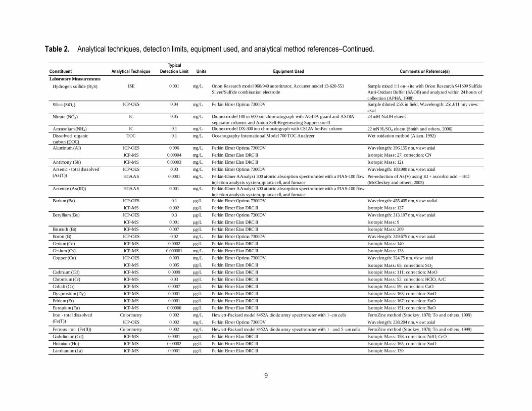
within the optimal range of the method. Table 2 lists the analytical techniques, detection limits,

equipment used, analytical method, and references for all constituents. Except for inductively coupled

plasma–mass spectrometry analyses and mercury determinations, detection limits were equal to three

times the standard deviation of several dozen measurements of the constituent in a blank solution

analyzed as a sample. The detection limits for inductively coupled plasma–mass spectrometry and cold

vapor atomic fluorescence spectrometry were determined using the method presented by Skogerboe and

Grant (1970). Details on the instrumentation, techniques, general conditions, and variants from standard

procedures are discussed in following sections.

.

8

Table 2. Analytical techniques, detection limits, equipment used, and analytical method references.

[cm, centimeter; CRDS, cavity ring-down spectroscopy; CVAFS, cold vapor atomic fluorescence spectrometry; °C, degrees Celsius; HCl, hydrochloric acid;

HGAAS, hydride generation atomic absorption spectrometry; IC, ion chromatography; ICP-OES, inductively coupled plasma-mass spectrometry; ICP-OES,

inductively coupled plasma-optical emission spectrometry; ISE, ion-selective electrode; KCl, potassium chloride; KI, potassium iodide; M, molar; mg/L,

micrograms per liter; mg/L, milligrams per liter; mM, millimolar; mN, millinormal; MS, mass spectrometry; N, normal; NaHCO3, sodium bicarbonate; Na2CO3,

sodium carbonate; ng/L, nanograms per liter; nm, nanometer; SLAP, standard light Antarctic precipitation; TISAB, total ionic strength adjustment buffer; TOC,

total organic carbon; VSMOW, Vienna standard mean ocean water; ≤, less than or equal to; %, percent] (Barnard and Nordstrom, 1982; Moses and others, 1984)

Constituent Analytical Technique

Typical

Detection Limit Units Equipment Used Comments or Reference(s)

Temperature Electronic sensor 0.1 °C Orion Research model 1230 multi-parameter meter with temperature sensor built

into conductivity electrode

Temperatures were reported to the nearest 0.1 °C

pH Potentiometry 0.02 pH units Orion 3-star meter with Orion Ross combination electrode Two- or three-buffer calibration at sample temperature using

1.68, 4.01, 7.00, and 10.00 pH buffers

Electrical Conductivity

(EC)

Conductometry 0.5 µS/cm Orion Research model 1230 multi-parameter meter with conductivity electrode Temperature correction to 25°C using the temperature

compensation method by McCleskey (2013), cell constant

determined with 0.010 N KCl

Eh Potentiometry 0.001 V Orion Research model 96-78-00 combination redox electrode Electrode checked using ZoBell's solution (ZoBell, 1946;

Nordstrom, 1977)

Dissolved oxygen (DO) Titration 0.1 mg/L Burette and Erlenmeyer flask Winkler Titration using manganous sulfate, alkaline iodide-

azide, sulfamic acid, starch indicator, phenyl arsine oxide

(APHA, 1971)

Laboratory Measurements

Calcium (Ca) ICP-OES 0.04 mg/L Perkin Elmer Optima 7300DV Wavelength: 317.933 nm, view: radial

Magnesium (Mg) ICP-OES 0.003 mg/L Perkin Elmer Optima 7300DV Wavelength: 285.211 nm, view: radial

ICP-MS 0.0001 mg/L Perkin Elmer Elan DRC II Isotopic Mass: 24.3

Sodium (Na) ICP-OES 0.08 mg/L Perkin Elmer Optima 7300DV Wavelength: 589.592 nm, view: radial

Potassium (K) ICP-OES 0.06 mg/L Perkin Elmer Optima 7300DV Wavelength: 766.495 nm view: axial

Alkalinity (as HCO3) Titration 1 mg/L Orion Research model 960/940 autotitrator, potentiometric detection, end-point

determined by the first derivative technique

(Barringer and Johnsson, 1996; Fishman and Friedman, 1989)

Chloride (Cl) IC 0.05 mg/L Dionex model 100 or 600 ion chromatograph with AG18A guard and AS18A

separator columns and Anion Self-Regenerating Suppressor-II

23 mM NaOH eluent

ISE 0.01 mg/L Orion Research model 96-09 combination F electrode Sample mixed 1:1 with Orion Research 940911 TISAB III

(Barnard and Nordstrom, 1980);

IC 0.1 mg/L Dionex model 100 or 600 ion chromatograph with AG18A guard and AS18A


23 mM NaOH eluent

Bromide (Br) IC 0.05 mg/L Dionex model 100 or 600 ion chromatograph with AG18A guard and AS18A


23 mM NaOH eluent

Sulfate (SO4) IC 0.1 mg/L Dionex model 100 or 600 ion chromatograph with AG18A guard and AS18A


23 mM NaOH eluent

Thiosulfate (S2O3) IC 0.1 mg/L Dionex model 100 ion chromatograph with two AG4A guard and an Anion Self-

Regenerating Suppressor-II

0.028 M NaHCO3 + 0.022 M Na2CO3 eluent (Moses and

others, 1984)

Polythionate (SnO6) IC 0.3 mg/L Dionex model 100 ion chromatograph with two AG4A guard and an Anion Self-

Regenerating Suppressor-II

0.028 M NaHCO3 + 0.022 M Na2CO3 eluent (Moses and

others, 1984)

Field Measurements

Fluoride (F)

9

Table 2. Analytical techniques, detection limits, equipment used, and analytical method references–Continued.


Typical


Hydrogen sulfide (H2S) ISE 0.001 mg/L Orion Research model 960/940 autotitrator, Accumet model 13-620-551

Silver/Sulfide combination electrode

Sample mixed 1:1 on–site with Orion Research 941609 Sulfide

Anti-Oxidant Buffer (SAOB) and analyzed within 24 hours of

collection (APHA, 1998)

Silica (SiO2) ICP-OES 0.04 mg/L Perkin Elmer Optima 7300DV Sample diluted 25X in field, Wavelength: 251.611 nm, view:

axial

Nitrate (NO3) IC 0.05 mg/L Dionex model 100 or 600 ion chromatograph with AG18A guard and AS18A


23 mM NaOH eluent

Ammonium (NH4) IC 0.1 mg/L Dionex model DX-300 ion chromatograph with CS12A IonPac column 22 mN H2SO4 eluent (Smith and others, 2006)

Dissolved organic

carbon (DOC)

TOC 0.1 mg/L Oceanography International Model 700 TOC Analyzer Wet oxidation method (Aiken, 1992)

ICP-OES 0.006 mg/L Perkin Elmer Optima 7300DV Wavelength: 396.155 nm, view: axial

ICP-MS 0.00004 mg/L Perkin Elmer Elan DRC II Isotopic Mass: 27; correction: CN

Antimony (Sb) ICP-MS 0.00003 mg/L Perkin Elmer Elan DRC II Isotopic Mass: 121


HGAAS 0.0001 mg/L Perkin-Elmer AAnalyst 300 atomic absorption spectrometer with a FIAS-100 flow

injection analysis system, quartz cell, and furnace

Pre-reduction of As(V) using KI + ascorbic acid + HCl

(McCleskey and others, 2003)

Arsenite (As(III)) HGAAS 0.001 mg/L Perkin-Elmer AAnalyst 300 atomic absorption spectrometer with a FIAS-100 flow

injection analysis system, quartz cell, and furnace

ICP-OES 0.1 µg/L Perkin Elmer Optima 7300DV Wavelength: 455.405 nm, view: radial

ICP-MS 0.002 µg/L Perkin Elmer Elan DRC II Isotopic Mass: 137

ICP-OES 0.3 µg/L Perkin Elmer Optima 7300DV Wavelength: 313.107 nm, view: axial


Bismuth (Bi) ICP-MS 0.007 µg/L Perkin Elmer Elan DRC II Isotopic Mass: 209

Boron (B) ICP-OES 0.02 mg/L Perkin Elmer Optima 7300DV Wavelength: 249.675 nm, view: axial

Cerium (Ce) ICP-MS 0.0002 µg/L Perkin Elmer Elan DRC II Isotopic Mass: 140

Cesium (Cs) ICP-MS 0.000001 mg/L Perkin Elmer Elan DRC II Isotopic Mass: 133


ICP-MS 0.005 µg/L Perkin Elmer Elan DRC II Isotopic Mass: 65; correction: SO2

Cadmium (Cd) ICP-MS 0.0009 µg/L Perkin Elmer Elan DRC II Isotopic Mass: 111; correction: MoO

Chromium (Cr) ICP-MS 0.03 µg/L Perkin Elmer Elan DRC II Isotopic Mass: 52; correction: HClO, ArC

Cobalt (Co) ICP-MS 0.0007 µg/L Perkin Elmer Elan DRC II Isotopic Mass: 59; correction: CaO

Dysprosium (Dy) ICP-MS 0.0001 µg/L Perkin Elmer Elan DRC II Isotopic Mass: 163; correction: SmO

Erbium (Er) ICP-MS 0.0001 µg/L Perkin Elmer Elan DRC II Isotopic Mass: 167; correction: EuO

Europium (Eu) ICP-MS 0.00006 µg/L Perkin Elmer Elan DRC II Isotopic Mass: 151; correction: BaO

Colorimetry 0.002 mg/L Hewlett-Packard model 8452A diode array spectrometer with 1–cm cells FerroZine method (Stookey, 1970; To and others, 1999)


Ferrous iron (Fe(II)) Colorimetry 0.002 mg/L Hewlett-Packard model 8452A diode array spectrometer with 1– and 5–cm cells FerroZine method (Stookey, 1970; To and others, 1999)

Gadolinium (Gd) ICP-MS 0.0001 µg/L Perkin Elmer Elan DRC II Isotopic Mass: 158; correction: NdO, CeO

Holmium (Ho) ICP-MS 0.00002 µg/L Perkin Elmer Elan DRC II Isotopic Mass: 165; correction: SmO

Lanthanum (La) ICP-MS 0.0001 µg/L Perkin Elmer Elan DRC II Isotopic Mass: 139

Copper (Cu)


Beryllium (Be)

Arsenic - total dissolved

(As(T))

Aluminum (Al)

Barium (Ba)

Iron - total dissolved

(Fe(T))

10

Table 2. Analytical techniques, detection limits, equipment used, and analytical method references–Continued.


Typical



ICP-MS 0.00009 mg/L Perkin Elmer Elan DRC II Isotopic Mass: 7

Lutetium (Lu) ICP-MS 0.00006 µg/L Perkin Elmer Elan DRC II Isotopic Mass: 175; correction: TbO



Mercury - total

dissolved (Hg(T))

CVAFS 0.4 ng/L PS Analytical, model Merlin Taylor and others (1997), Roth and others (2001)

ICP-OES 3 µg/L Perkin Elmer Optima 7300DV Wavelength: 202.031 nm, view: axial


Neodymium (Nd) ICP-MS 0.0003 µg/L Perkin Elmer Elan DRC II Isotopic Mass: 146

Nickel (Ni) ICP-MS 0.003 µg/L Perkin Elmer Elan DRC II Isotopic Mass: 60; correction: CaO, CaC

Lead (Pb) ICP-MS 0.003 µg/L Perkin Elmer Elan DRC II Isotopic Mass: composite of 206, 207, 208


ICP-MS 1 µg/L Perkin Elmer Elan DRC II Isotopic Mass: 31

Praseodymium (Pr) ICP-MS 0.00005 µg/L Perkin Elmer Elan DRC II Isotopic Mass: 141

Rhenium (Re) ICP-MS 0.00008 µg/L Perkin Elmer Elan DRC II Isotopic Mass: 187; correction: YbO

Rubidium (Rb) ICP-OES 2 µg/L Perkin Elmer Optima 7300DV Wavelength: 780.025 nm, view: axial

Samarium (Sm) ICP-MS 0.0003 µg/L Perkin Elmer Elan DRC II Isotopic Mass: 147

Selenium (Se) ICP-MS 0.08 µg/L Perkin Elmer Elan DRC II Isotopic Mass: 77; correction: ArCl

ICP-OES 0.001 mg/L Perkin Elmer Optima 7300DV Wavelength: 407.771 nm, view: radial


Tin (Sn) ICP-MS 0.08 µg/L Perkin Elmer Elan DRC II Isotopic Mass: 118

Terbium (Tb) ICP-MS 0.00004 µg/L Perkin Elmer Elan DRC II Isotopic Mass: 159; correction: NdO

Tellurium (Te) ICP-MS 0.004 µg/L Perkin Elmer Elan DRC II Isotopic Mass: 126

Thorium (Th) ICP-MS 0.001 µg/L Perkin Elmer Elan DRC II Isotopic Mass: 232

Thallium (Tl) ICP-MS 0.0006 µg/L Perkin Elmer Elan DRC II Isotopic Mass: 205

Thulium ( Tm) ICP-MS 0.00007 µg/L Perkin Elmer Elan DRC II Isotopic Mass: 169: correction: EuO

Tungsten (W) ICP-MS 0.1 µg/L Perkin Elmer Elan DRC II Isotopic Mass: 182; correction: ErO

Uranium (U) ICP-MS 0.0002 µg/L Perkin Elmer Elan DRC II Isotopic Mass: 238


ICP-MS 0.008 µg/L Perkin Elmer Elan DRC II Isotopic Mass: 51; correction: ClO

Yttrium (Y) ICP-MS 0.0001 µg/L Perkin Elmer Elan DRC II Isotopic Mass: 89

Ytterbium (Yb) ICP-MS 0.00009 µg/L Perkin Elmer Elan DRC II Isotopic Mass: 174; correction: GdO


ICP-MS 0.02 µg/L Perkin Elmer Elan DRC II Isotopic Mass: 66; correction: Ba++

Zirconium (Zr) ICP-MS 0.0006 µg/L Perkin Elmer Elan DRC II Isotopic Mass: 90

Deuterium (δD) CRDS 0.11 ‰ Los Gatos Research – Liquid Water Isotope Analyzer Standardization against VSMOW (δD = 0 per mil)

Oxygen (δ18

O) CRDS 0.11 ‰ Los Gatos Research – Liquid Water Isotope Analyzer Standardization against VSMOW (δ

18O = 0 per mil)

Acidity (total/free H+) Titration 0.4 mN Orion Research model 960/940 autotitrator, potentiometric detection (Barringer and Johnsson, 1996)

1 Relative standard deviation expressed in percent

Phosphorus (P)


Zinc (Zn)

Vanadium (V)

Molybdenum (Mo)

Strontium (Sr)

Lithium (Li)

Manganese (Mn)

11

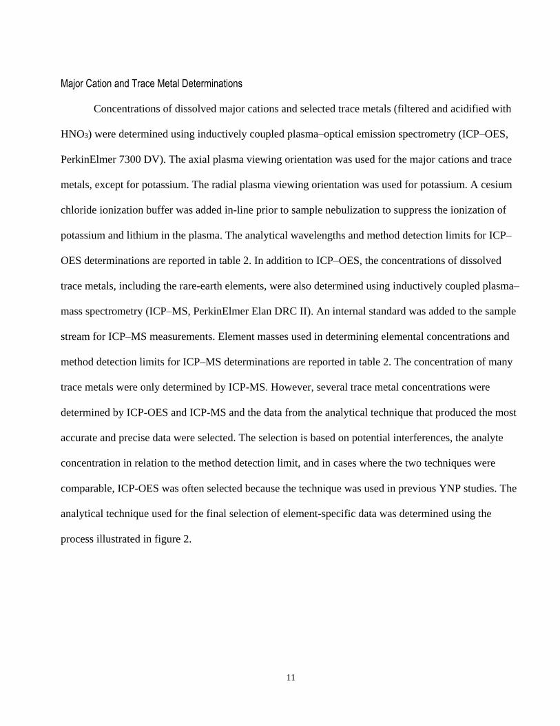
Major Cation and Trace Metal Determinations

Concentrations of dissolved major cations and selected trace metals (filtered and acidified with

HNO3) were determined using inductively coupled plasma–optical emission spectrometry (ICP–OES,

PerkinElmer 7300 DV). The axial plasma viewing orientation was used for the major cations and trace

metals, except for potassium. The radial plasma viewing orientation was used for potassium. A cesium

chloride ionization buffer was added in-line prior to sample nebulization to suppress the ionization of

potassium and lithium in the plasma. The analytical wavelengths and method detection limits for ICP–

OES determinations are reported in table 2. In addition to ICP–OES, the concentrations of dissolved

trace metals, including the rare-earth elements, were also determined using inductively coupled plasma–

mass spectrometry (ICP–MS, PerkinElmer Elan DRC II). An internal standard was added to the sample

stream for ICP–MS measurements. Element masses used in determining elemental concentrations and

method detection limits for ICP–MS determinations are reported in table 2. The concentration of many

trace metals were only determined by ICP-MS. However, several trace metal concentrations were

determined by ICP-OES and ICP-MS and the data from the analytical technique that produced the most

accurate and precise data were selected. The selection is based on potential interferences, the analyte

concentration in relation to the method detection limit, and in cases where the two techniques were

comparable, ICP-OES was often selected because the technique was used in previous YNP studies. The

analytical technique used for the final selection of element-specific data was determined using the

process illustrated in figure 2.

12

Figure 2. Flow-chart for the analytical technique used for the final selection of element-specific data.

Anion and Alkalinity Determinations

Concentrations of bromide, chloride, fluoride, nitrate, and sulfate were determined by ion

chromatography (IC, Dionex DX 600) with suppressed electrical conductivity detection (Brinton and

others, 1995). An IonPac AS18 Analytical Column (4 mm), AG18 Guard Column, and an Anion Self-

Regenerating Suppressor (ASRS ULTRA II (4 mm)) were used. Thirty-millimolar sodium hydroxide

(NaOH) eluent was pumped through the columns at 1 milliliter per minute (mL/min). Analytical errors

for these constituents are typically less than 5 percent. The ion chromatography method detection limits

Are both ICP-MS and ICP-OES data

available?

No ICP-MS data

No ICP-OES data

Report ICP-OES data [B, Ca, Na, K, Li, SiO2]

Report ICP-MS data[Bi, Ce, Cs, Dy, Er, Eu, Gd, Ho, La, Lu, Nd, Pr, Re, Sm, Sn, Tb, Te, Th, Tl, Tm, Y, Yb, Zr]

Yes

Are there any interferences with ICP-MS analysis?

No

Yes

Are all ICP-OES values <20 times

detection limit for that element?

Yes

Report ICP-MS data [Cd, Co, Cr, Cu, Pb, U, Sb]

As (Cl interference): Report ICP-OES, HGAASSe (Cl, Br interferences): Report ICP-MS data with fewer significant figures for high Cl, Br samples to reflect analytical uncertaintyV (Cl interference): Report ICP-OES

NoReport ICP-OES data unless concentration is <20 times detection limit, then report ICP-MS data [Al, B, Ba, Be, Mg, Mn, Mo, Ni, Sr, Rb, Zn, P, V]

13

are reported in the accompanying Microsoft Excel spreadsheet in the "Analytical" worksheet. Samples

for F determination by ISE were mixed 1:1 with a total ionic strength adjustment buffer (TISAB III)

(Barnard and Nordstrom, 1980).

Alkalinity was determined by automated titration (Thermo, 940-960 autotitrator) using

standardized sulfuric acid (Barringer and Johnsson, 1996; Fishman and Friedman, 1989). Fifteen

milliliters of sample were titrated with 0.01 normal (equivalents per liter) sulfuric acid to the

bicarbonate end-point. The analytical error in alkalinity concentrations is less than 3 percent.

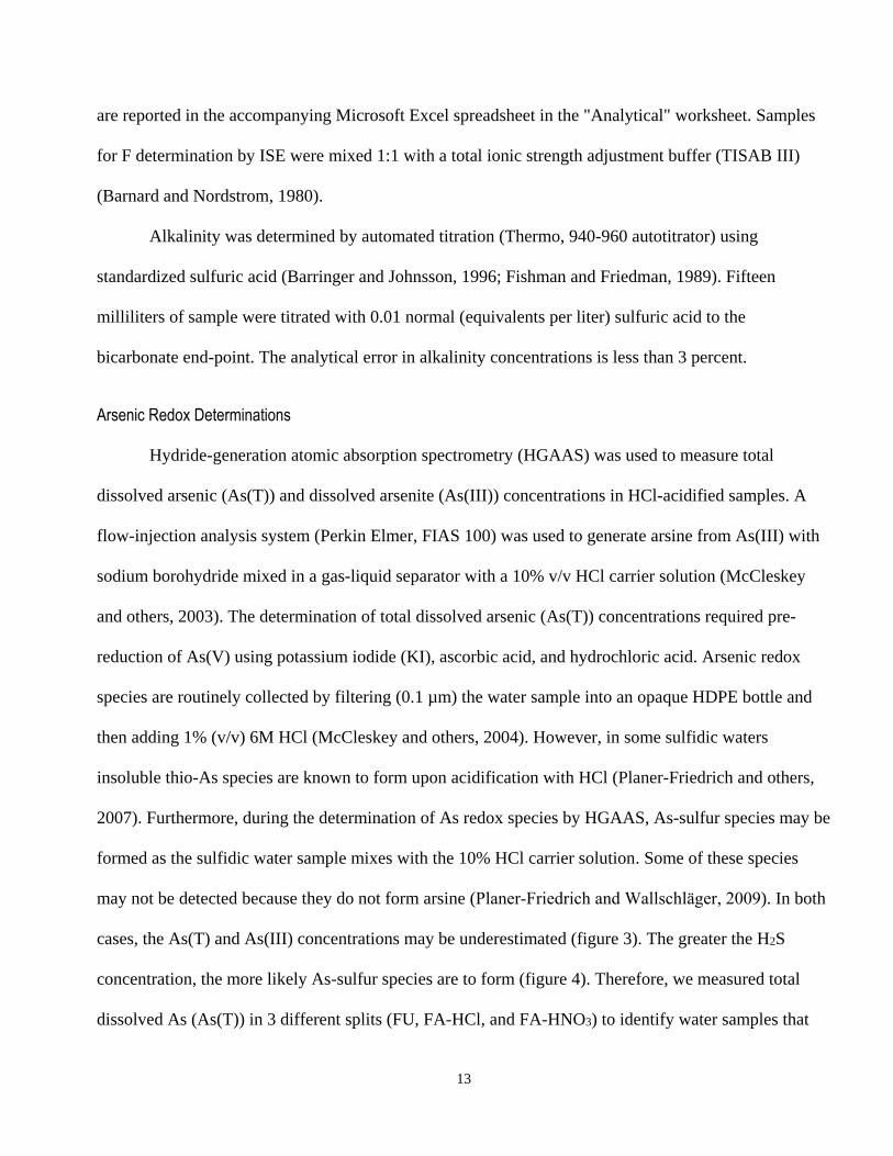
Arsenic Redox Determinations

Hydride-generation atomic absorption spectrometry (HGAAS) was used to measure total

dissolved arsenic (As(T)) and dissolved arsenite (As(III)) concentrations in HCl-acidified samples. A

flow-injection analysis system (Perkin Elmer, FIAS 100) was used to generate arsine from As(III) with

sodium borohydride mixed in a gas-liquid separator with a 10% v/v HCl carrier solution (McCleskey

and others, 2003). The determination of total dissolved arsenic (As(T)) concentrations required pre-

reduction of As(V) using potassium iodide (KI), ascorbic acid, and hydrochloric acid. Arsenic redox

species are routinely collected by filtering (0.1 µm) the water sample into an opaque HDPE bottle and

then adding 1% (v/v) 6M HCl (McCleskey and others, 2004). However, in some sulfidic waters

insoluble thio-As species are known to form upon acidification with HCl (Planer-Friedrich and others,

2007). Furthermore, during the determination of As redox species by HGAAS, As-sulfur species may be

formed as the sulfidic water sample mixes with the 10% HCl carrier solution. Some of these species

may not be detected because they do not form arsine (Planer-Friedrich and Wallschlager, 2009). In both

cases, the As(T) and As(III) concentrations may be underestimated (figure 3). The greater the H2S

concentration, the more likely As-sulfur species are to form (figure 4). Therefore, we measured total

dissolved As (As(T)) in 3 different splits (FU, FA-HCl, and FA-HNO3) to identify water samples that

14

form thio-As species upon acidification with HCl or during measurement by HGAAS. The As(T)

determined by ICP-OES in the FA-HNO3 sample split is considered to be the most accurate because

HNO3 is known to oxidize redox species and inhibit the formation of thio-As species. Thus, we used the

As(T) measured in the FA-HNO3 as a guide to identify the samples that likely form thio-As species

upon acidification with HCl or measurement by HGAAS. In cases where the measurements of the

various splits are within the analytical error (~±10%), formation of thio-As species was not significant

and the As(T) concentrations and As(III) concentrations reported are from the FA-HCl split determined

with HGAAS. However, in the cases where the As(T) concentration in the FA-HNO3 split was found to

be ≥110% of the As(T) concentration in the FA-HCl, it was concluded that thio-As species had formed

and that the As(T) and As(III) concentrations measured in the FA-HCl split were biased low. For these

fifty samples, the reported As(T) concentration is from the FA-HNO3 split. The As(III) concentrations

are from the HCl split and reported as minimum values with a “≥” symbol. The As(T) and As(III) in the

remaining samples were reported for the FA-HCl split.

0 1 2 3 4 5 6 7 80

1

2

3

4

5

6

7

8

HG

AA

S

ICP-OES

As(T), mg/L

Figure 3. As(T) concentrations determined by HGAAS in the FA-HCl split plotted against As(T) concentrations

determined by ICP-OES in the FA-HNO3 split.

15

1E-3 0.01 0.1 1-80

-60

-40

-20

0

20

40

% D

iffe

ren

ce (

HG

AA

S -

IC

P-O

ES

)

H2S, mg/L

Figure 4. The percent differences in the measured As concentrations plotted against H2S concentrations.

Iron Redox Determinations

Total dissolved iron (Fe(T)) and ferrous iron (Fe(II)) concentrations (filtered and acidified with

HCl) were determined in samples preserved with HCl using a modification of the FerroZine

colorimetric method (Gibbs, 1976; Stookey, 1970; To and others, 1999). All iron determinations were

prepared in 25-mL volumetric flasks and then their absorbances were measured at 562 nm using a diode

array spectrometer (Hewlett-Packard model 8452A). For total dissolved iron determinations,

hydroxylamine hydrochloride was first added to the sample to pre-reduce any ferric iron, then the

FerroZine reagent and acetate buffer were added. Ferrous iron was determined by only adding

FerroZine reagent and acetate buffer.

Ammonium Determinations

Concentrations of ammonium (filtered and acidified with H2SO4) were determined by ion

chromatography (Dionex DX 300) with suppressed electrical conductivity detection. An IonPac AS12A

Analytical Column (4mm), an AG12A Guard Column, and a Cation Self-Regenerating Suppressor

16

(CSRS 300 (4-mm)) were used. A gradient pump was used to pump sulfuric acid (H2SO4) eluent

through the system. The method detection limit was 0.04 milligrams per liter (mg/L).

Mercury Determinations

Total dissolved mercury (Hg) concentrations (filtered and preserved with HNO3/K2Cr2O7) for a

subset of samples were determined by direct cold-vapor atomic fluorescence spectroscopy (CVAFS)

using the method of Roth and others (2001). Samples are oxidized using potassium dichromate, then

reduced by stannous chloride, followed by atomic fluorescence detection. The method detection limit

was 0.4 nanograms per liter.

Dissolved Organic Carbon

Dissolved organic carbon (DOC) concentrations were measured using the wet oxidation method

(Aiken, 1992) with an Oceanography International Model 700 TOC Analyzer. Potassium biphthalate

was used to calibrate the instrument, and sodium benzoate was used as a different organic carbon source

to check the calibration. The method detection limit for DOC was 0.4 mg/L.

Water Isotope Determinations

Hydrogen and oxygen isotope ratios were determined at the USGS Laboratory in Boulder, CO

using cavity ring-down spectroscopy (CRDS - Los Gatos Research – Liquid Water Isotope Analyzer).

The isotopic concentration is reported in “delta notation,” which compares the isotope ratio of a sample

to that of a reference standard. For the example of 18O/16O ratios, delta notation was determined with the

following equation:

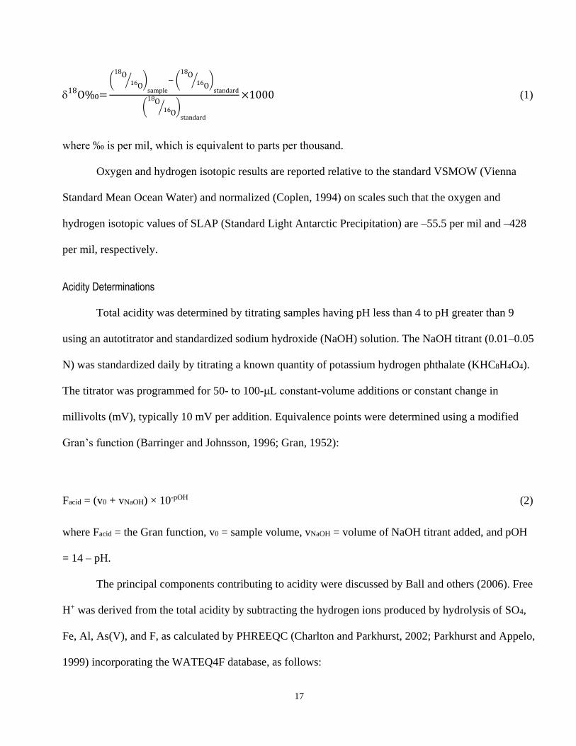
17

d18O‰=

(O18

O16⁄ )sample

− (O18

O16⁄ )standard

(O18

O16⁄ )standard

×1000 (1)

where ‰ is per mil, which is equivalent to parts per thousand.

Oxygen and hydrogen isotopic results are reported relative to the standard VSMOW (Vienna

Standard Mean Ocean Water) and normalized (Coplen, 1994) on scales such that the oxygen and

hydrogen isotopic values of SLAP (Standard Light Antarctic Precipitation) are –55.5 per mil and –428

per mil, respectively.

Acidity Determinations

Total acidity was determined by titrating samples having pH less than 4 to pH greater than 9

using an autotitrator and standardized sodium hydroxide (NaOH) solution. The NaOH titrant (0.01–0.05

N) was standardized daily by titrating a known quantity of potassium hydrogen phthalate (KHC8H4O4).

The titrator was programmed for 50- to 100-μL constant-volume additions or constant change in

millivolts (mV), typically 10 mV per addition. Equivalence points were determined using a modified

Gran’s function (Barringer and Johnsson, 1996; Gran, 1952):

Facid = (v0 + vNaOH) × 10-pOH (2)

where Facid = the Gran function, v0 = sample volume, vNaOH = volume of NaOH titrant added, and pOH

= 14 – pH.

The principal components contributing to acidity were discussed by Ball and others (2006). Free

H+ was derived from the total acidity by subtracting the hydrogen ions produced by hydrolysis of SO4,

Fe, Al, As(V), and F, as calculated by PHREEQC (Charlton and Parkhurst, 2002; Parkhurst and Appelo,

1999) incorporating the WATEQ4F database, as follows:

18

AciditySO4

=HSO4- (3)

AcidityFe

=3(FeIII(tot)-Fe(OH)2

+)+2FeOH2++Fe(OH)

2

++2FeII(tot) (4)

AcidityAl

=3(Al(tot)-AlOH2+-Al(OH)2+)+2AlOH2++Al(OH)2

+ (5)

AcidityAs

=2(AsV(tot)-H2AsO4- )+H2AsO4

- (6)

AcidityF=HF0 (7)

AcidityH+=Acidity

Total-Acidity

SO4-Acidity

Fe-Acidity

Al-Acidity

As-Acidity

F (8)

Concentrations for the above equations are expressed in moles per kilogram of water. Sample

pH from the acidity titration (acidity pH) was calculated by computing the product of the H+ activity

coefficient (calculated by PHREEQCi) and the free H+ molality (equation 8) and computing the

negative common logarithm of the resulting activity. This pH value was refined by repeating the

PHREEQCi calculation and varying the input pH until the pH calculated from the PHREEQCi

speciation was equal to the input pH. A flow-chart illustrating the process for refining the acidity pH is

shown in figure 5.

19

Figure 5. Flow chart illustrating the process for refining the acidity pH value.

Revised pH Measurements

Accurate measurement of pH is of primary importance for interpreting aqueous chemical

speciation. The free hydrogen ion (H+) is usually the major cation in samples with pH less than 2.5 in

geothermal waters (Ball and others, 2002), is important in controlling geochemical reactions, and is

20

critical in calculating the charge imbalance (C.I.) for waters with pH less than 3. For the subset of 208

samples with pH less than 4, pH values determined using three different techniques were evaluated: (1)

pH measured in the field; (2) pH measured in the laboratory; (3) acidity pH (calculated as discussed in

the previous section). Comparison of pH values from the three sources allows evaluation of the

measurements and estimation of more accurate pH values.

A flow chart showing the pH selection process is shown in figure 6. Field pH is considered to be

the most accurate because pH measurements made in the laboratory may be biased from temperature

changes and hydrolysis reactions, and the acidity pH calculation relies on measurements of SO4, Fe, Al,

As, and F, all of which are subject to analytical uncertainties, temperature changes, and hydrolysis

reactions.

For samples having a pH less than 3.5, field pH was selected unless the sample had a speciated

C.I. greater than 10 percent using field pH. For samples with pH less than 3.5 and speciated C.I. greater

than 10 percent using field pH, laboratory pH was selected if the speciated C.I. was less than 10 percent.

For samples with pH less than 3.5 and speciated C.I. greater than 10 percent using both field and

laboratory pH, acidity pH was selected if the speciated C.I. was less than 10 percent. For samples with

pH less than 3.5 and having field, laboratory, and acidity pH values that all produced speciated C.I.s

greater than 10 percent, the pH that produced the lowest speciated C.I. was selected from among field,

laboratory, and acidity pH.

Using the process described above and illustrated in figure 6 for the subset of 190 samples with a

field pH less than 3.5, field pH was selected for 140 samples, laboratory pH was selected for 43

samples, and acidity pH was selected for 7 samples. Values of the selected pH are found in the table of

chemical data along with the speciated C.I. calculated using the selected pH and field temperature.

21

Figure 6. Flow chart showing the pH selection process. (C.I., charge imbalance)

22

Quality Assurance and Quality Control

Several techniques were used to assure the quality of the ionic analytical data. These techniques

included calculation of charge imbalance, electrical conductivity balance, analysis of blanks, analyses

by alternate methods, analysis of U.S. Geological Survey SRWS, and analysis of replicate samples.

The charge imbalance calculation is a common quality-assurance/quality-control procedure to

check the accuracy of a water analysis (APHA, American Public Health Association, 1971). For

samples that were analyzed for major cations and anions, the accuracy of the analyses were checked for

charge imbalance using the geochemical code WATEQ4F (Ball and Nordstrom, 1991). WATEQ4F uses

equation 9 to calculate charge imbalance:

𝐶ℎ𝑎𝑟𝑔𝑒 𝑖𝑚𝑏𝑎𝑙𝑎𝑛𝑐𝑒 (𝑝𝑒𝑟𝑐𝑒𝑛𝑡) = (𝑠𝑢𝑚 𝑐𝑎𝑡𝑖𝑜𝑛𝑠−𝑠𝑢𝑚 𝑎𝑛𝑖𝑜𝑛𝑠)

(𝑠𝑢𝑚 𝑐𝑎𝑡𝑖𝑜𝑛𝑠+𝑠𝑢𝑚 𝑎𝑛𝑖𝑜𝑛𝑠)÷2× 100 (9)

where sum cations and sum anions are in milliequivalents per liter (meq/L). The charge balance

calculation is discussed in more detail by Ball and others (2006). The charge imbalance, sum cations

(meq/L), and sum anions (meq/L) are reported for all samples having major cation and anion

determinations. A frequency plot of charge imbalance for all samples with complete analyses is shown

in figure 7. The mean charge imbalance was -1.1 percent with a standard deviation of 4.8 percent.

Analyses having a charge imbalance less than ±10 percent are considered reliable for speciation

calculations (Nordstrom and Munoz, 1994). Two sample analyses, out of 351, had charge imbalances

greater than ±10 percent. However, charge imbalance does not indicate whether the error is caused by a

cation or an anion. Therefore, a second constraint is needed to identify the constituent most likely in

error. By coupling charge imbalance and electrical conductivity imbalance, the measurement most likely

in error can be identified or narrowed down to a few possibilities (McCleskey and others, 2012). A plot

of electrical conductivity imbalance against charge imbalance for these samples shows that the electrical

23

conductivity imbalance was within ±10 percent for all but 7 samples (figure 8).

-40 -30 -20 -10 0 10 20 30 400

10

20

30

40

50

60

FR

EQ

UE

NC

Y

CHARGE IMBALANCE, IN PERCENT

Mean = -1.1%

Median = -1.5%

Figure 7. Frequency distribution of charge imbalance for samples having major cation and anion determinations.

-40 -30 -20 -10 0 10 20 30 40-30

-20

-10

0

10

20

30

Cations Too High

Anions Too LowCations Too Low

WA samples

Y10G samples

ELE

CT

RIC

AL C

ON

DU

CT

IVIT

Y I

MB

AL

AN

CE

, IN

PE

RC

EN

T

CHARGE IMBALANCE, IN PERCENT

Anions Too High

Figure 8. Electrical conductivity imbalance compared with charge imbalance.

24

Eight field blanks were analyzed along with the samples as unknowns. Field blanks were

deionized water that was filtered and preserved in the same manner as the samples. Constituents were

below detection in all these blanks, with a few exceptions. Chloride was detected in all the blanks, most

likely from HCl used to wash the filter apparatus; the highest Cl concentration was 1.8 mg/L. Sulfate

was detected in 3 blanks, the highest being 1.5 mg/L, most likely from small amounts of contamination

within the IC columns. Trace amounts of SiO2 (<0.4 mg/L) were detected in all samples, originating

either from contaminated blank deionized water or from incompletely cleaned filters. Dissolved organic

carbon was detected in all 3 blanks, the highest being 1.3 mg/L, most likely because of organic carbon

in the deionized blank water. Apart from dissolved organic carbon, the constituents measured in the

blanks were less than the typical error associated with the analyses and are a small fraction of the

measured concentrations.

Concentrations of Al, As, B, Ba, Be, Cd, Co, Cr, Cu, F, Fe, Li, Mg, Mn, Mo, Ni, P, Pb, Rb, Sb,

Sr, U, V, W, and Zn were determined by more than one method. Comparing analytical results from

alternative methods can serve as an accuracy check, although in all cases one method was preferred over

the others depending on sample matrix and proximity to the method detection limit (figure 2).

Concentrations of Al, As, B, Ba, Be, Cd, Co, Cr, Cu, Li, Mg, Mn, Mo, Ni, P, Pb, Rb, Sb, Sr, U, V, W,

and Zn were determined by ICP-OES and ICP-MS (figure 9). Concentrations of Fe were determined by

ICP-OES and by the FerroZine method (figure 10). The reported data were obtained using the preferred

method unless there was insufficient sample volume to perform the determinations.

Comparison of analytical results for cations and trace metals from the ICP-OES and ICP-MS are

in good agreement except for some low-level concentrations and high Al concentrations. Low-level

concentrations of Cd, Cu, Ni, Pd, U, and Zn are likely overestimated by ICP-OES (figure 9) because the

analyte concentration is near the detection limit. In the case of Cd, elevated As concentrations interfere

25

with the Cd determination. For the low-level concentrations of Cd, Cu, Ni, Pd, U, and Zn the

concentration determined by ICP-MS was the preferred value (figure 2). Aluminum concentrations in

some samples (Al > 2 mg/L) determined by ICP-MS are lower than the concentrations determined by

ICP-OES by more than 10%. The accuracy of both techniques is thought to be good at these

concentrations, but the ICP-OES values were selected (figure 2) in part because the ICP-MS is

optimized for low-level determinations and a large dilution was required to bring the Al concentration

into the ICP-MS calibration range.

Concentrations of Fe by FerroZine were determined on a subsample preserved with HCl,

whereas Fe concentrations determined by ICP-OES were determined on a subsample preserved with

HNO3 (figure 10). The uncertainty line was calculated based on the method with the higher detection

limit. At the method detection limit the uncertainty is ±100 percent and decreases to ±5 percent at 20

times the detection limit (quantitation limit). With only a few exceptions, Fe concentrations determined

by FerroZine and by ICP-OES are in good agreement. When available, results for Fe are reported for the

sample preserved with HCl because the redox species concentrations were obtained from this split.

Considering the uncertainty of the measurements and that the analyses were performed on different

splits, analytical results for total dissolved Fe obtained by the alternative methods are in good

agreement.

26

0 5 10 15 20 25 30

0

5

10

15

20

25

30

0.01 0.1 1 10 100 1000 10000 100000

0.01

0.1

1

10

100

1000

10000

100000

CO

NC

EN

TR

AT

ION

IN

MIL

LIG

RA

MS

PE

R L

ITE

R

AN

ALY

SE

S B

Y IC

P-M

S

CONCENTRATION IN MILLIGRAMS PER LITER

ANALYSES BY ICP-OES

A.

B.

Al, As, B, Ba, Be, Cd, Co, Cr

Cu, Li, Mg, Mn, Mo, Ni, P, Pb

Rb, Sb, Sr, U, V, W, Zn

CO

NC

EN

TR

AT

ION

IN

MIC

RO

GR

AM

S P

ER

LIT

ER

AN

ALY

SE

S B

Y IC

P-M

S

CONCENTRATION IN MICROGRAMS PER LITER

ANALYSES BY ICP-OES

Figure 9. Cation and trace metals concentrations determined by ICP-MS and ICP-OES plotted on a linear (A) and

log10 (B) scale. The solid line is a one to one concentration line and the dashed lines are ±10%.

27

0 20 40 60 80 100

0

20

40

60

80

100

0 1 2 3 4 5

0

1

2

3

4

5

IRO

N C

ON

CE

NT

RA

TIO

N I

N M

ILLIG

RA

MS

PE

R L

ITE

R

DE

TE

RM

INE

D B

Y IC

P-O

ES

IRON CONCENTRATION IN MILLIGRAMS PER LITER

DETERMINED BY FERROZINE

A. B.

IRO

N C

ON

CE

NT

RA

TIO

N I

N M

ILLIG

RA

MS

PE

R L

ITE

R

DE

TE

RM

INE

D B

Y IC

P-O

ES

IRON CONCENTRATION IN MILLIGRAMS PER LITER

DETERMINED BY FERROZINE

Figure 10. Total dissolved iron determined by ICP-OES and FerroZine for all data (A) and for iron concentrations

less than 5 mg/L (B). The solid line is a one to one concentration line and the dashed lines are ±10%.

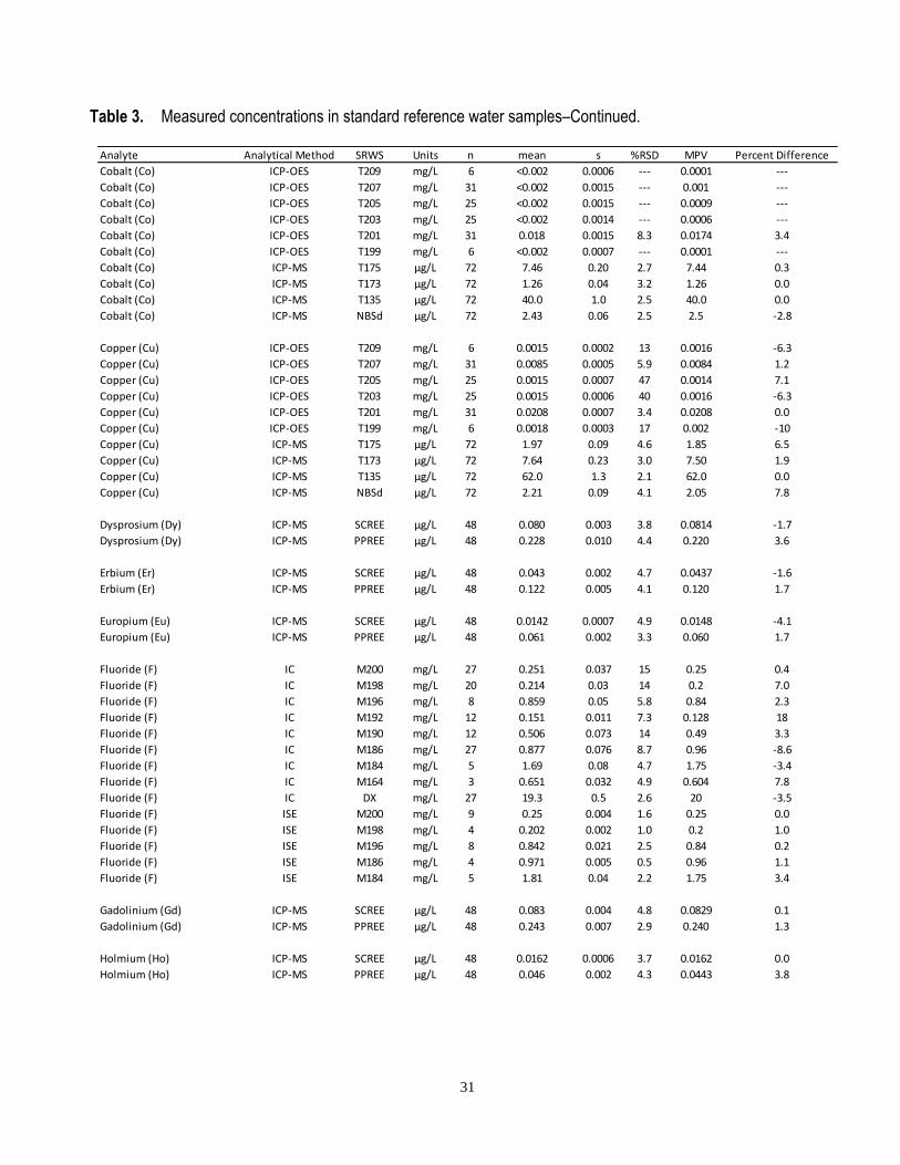
Several standard reference water samples were analyzed as unknowns several times during each

analytical run to check for accuracy. U.S. Geological Survey standard reference water samples (SRWS)

M158, M164, M184, M186, M190, M192, M196, M198, M200, M202, M204, N103, N104, N106,

N107, N108, N111, N112, T135, T173, T175, T181, T189, T195, T199, T201, T203, T205, T207,

T209, Hg08, Hg21, and Hg27 (U.S. Geological Survey, 2013) were used to check the analytical

methods for major and trace metals, ammonium, anions, and mercury. The SRWS PPREE and SCREE

were used to check the analytical methods for rare earth elements (Verplanck and others, 2001). The

National Institute of Standards and Technology (NIST) standard NIST1643d (NIST, 1999) was used to

check the accuracy of trace metals determined by ICP-MS. The Environment Canada standards

FP99Hg05, FP97Hg09, FP97Hg06, FP97Hg04, FP97Hg03, FP97Hg01, FP95Hg09, FP95Hg06,

FP95Hg05, FP95Hg03, FP93Hg10, FP93Hg06, FP85Hg03, and FP81Hg10 were used to check the

CVAFS determination of Hg (Environment Canada, 2014). For each SRWS constituent, the analytical

result, the most probable value (MPV), and the percent difference are presented in table 3.

28

Table 3. Measured concentrations in standard reference water samples.

[CVAFS, cold vapor atomic fluorescence spectrometry; HGAAS, hydride generation atomic absorption spectrometry; IC,

ion chromatography; ICP-OES, inductively coupled plasma-optical emission spectrometry; ISE, ion selective electrode;

mg/L, milligrams per liter; n, number of analyses; ng/L, nanograms per liter; s, standard deviation; SRWS, standard

reference water sample; %RSD, percent relative standard deviation; <, less than; ---, no data]

Analyte Analytical Method SRWS Units n mean s %RSD MPV Percent Difference

Alkalinity (as CaCO3) Titration M204 mg/L 4 40.9 0.4 1.0 40.9 -0.1

Alkalinity (as CaCO3) Titration M200 mg/L 2 28.6 0.1 0.3 28.3 1.1


Alkalinity (as CaCO3) Titration M192 mg/L 6 23.5 0.7 3.0 24 -2.1


Alkalinity (as CaCO3) Titration M184 mg/L 8 43.2 0.7 1.6 43.5 -0.7

Alkalinity (as CaCO3) Titration M158 mg/L 1 64.1 --- --- 63.6 0.8

Aluminum (Al) ICP-OES T209 mg/L 6 0.0192 0.0012 6.3 0.0192 0.0


Aluminum (Al) ICP-OES T205 mg/L 25 0.0299 0.0017 5.7 0.0315 -5.1




Aluminum (Al) ICP-MS T175 µg/L 72 51.3 2.5 4.9 52.0 -1.3

Aluminum (Al) ICP-MS T173 µg/L 72 71.8 3.3 4.6 71.0 1.1

Aluminum (Al) ICP-MS T135 µg/L 72 10.3 1.2 11.7 10.5 -1.9

Aluminum (Al) ICP-MS NBSd µg/L 72 12.8 1.1 8.6 12.8 0.0

Ammonium (as NH3-N) IC N103 mg/L 1 0.345 --- --- 0.320 7.8

Ammonium (as NH3-N) IC N104 mg/L 0 0.663 0.051 7.7 0.705 -6.0

Ammonium (as NH3-N) IC N106 mg/L 1 1.04 --- --- 1.10 -5.5

Ammonium (as NH3-N) IC N107 mg/L 0 0.214 0.011 5.1 0.193 10.9




Antimony (Sb) ICP-OES T209 mg/L 6 <0.01 0.0065 --- 0.0003 ---






Antimony (Sb) ICP-MS T175 µg/L 72 1.98 0.16 8.1 1.90 4.2

Antimony (Sb) ICP-MS T173 µg/L 72 5.04 0.09 1.8 5.20 -3.1

Antimony (Sb) ICP-MS T135 µg/L 72 76.3 0.9 1.2 76.3 0.0

Antimony (Sb) ICP-MS NBSd µg/L 72 5.31 0.10 1.9 5.41 -1.8

29

Table 3. Measured concentrations in standard reference water samples–Continued.


Arsenic (As) HGAAS T207 mg/L 2 0.0007 0 0.0 0.0009 -22

Arsenic (As) HGAAS T201 mg/L 7 0.0244 0.0011 4.5 0.0244 0.0

Arsenic (As) HGAAS T195 mg/L 3 0.0014 0 0.0 0.0015 -6.7

Arsenic (As) HGAAS AMW4 mg/L 81 0.178 0.008 4.5 0.168 6.0

Arsenic (As) ICP-OES T209 mg/L 6 <0.03 --- --- 0.0002 ---






Arsenic (As) ICP-MS T175 µg/L 72 7.40 0.14 1.9 7.38 0.3

Arsenic (As) ICP-MS T173 µg/L 72 2.63 0.13 4.9 2.67 -1.5

Arsenic (As) ICP-MS T135 µg/L 72 10.2 0.2 2.0 10.0 2.0

Arsenic (As) ICP-MS NBSd µg/L 72 5.17 0.16 3.1 5.60 -7.7

Barium (Ba) ICP-OES T209 mg/L 6 0.0315 0.0003 1.0 0.0316 -0.3

Barium (Ba) ICP-OES T207 mg/L 31 0.0435 0.0012 2.8 0.0429 1.4



Barium (Ba) ICP-OES T201 mg/L 31 0.0445 0.0012 2.7 0.0447 -0.4


Barium (Ba) ICP-MS T175 µg/L 72 17.9 0.5 2.8 18.0 -0.6

Barium (Ba) ICP-MS T173 µg/L 72 41.4 1.3 3.1 42.2 -1.9

Barium (Ba) ICP-MS T135 µg/L 72 68.0 1.5 2.2 67.8 0.3

Barium (Ba) ICP-MS NBSd µg/L 72 50.7 1.3 2.6 50.7 0.0

Beryllium (Be) ICP-OES T209 mg/L 6 <0.0001 0 --- 0.0001 ---

Beryllium (Be) ICP-OES T207 mg/L 31 <0.0001 0.0001 --- 0.0001 ---

Beryllium (Be) ICP-OES T205 mg/L 25 0.0002 0.0001 50 0.0002 0.0

Beryllium (Be) ICP-OES T203 mg/L 25 0.0006 0.0001 17 0.0005 20

Beryllium (Be) ICP-OES T201 mg/L 31 0.0084 0.0003 3.6 0.0084 0.0

Beryllium (Be) ICP-OES T199 mg/L 6 <0.0001 0.0001 --- 0.0001 ---

Beryllium (Be) ICP-MS T175 µg/L 72 2.96 0.10 3.4 2.92 1.4

Beryllium (Be) ICP-MS T173 µg/L 72 2.02 0.09 4.5 2.00 1.0

Beryllium (Be) ICP-MS T135 µg/L 72 58.9 2.2 3.7 59.0 -0.2

Beryllium (Be) ICP-MS NBSd µg/L 72 1.18 0.06 5.1 1.25 -5.6

Bismuth (Bi) ICP-MS NBSd µg/L 72 1.29 0.04 3.1 1.30 -0.8

Boron (B) ICP-OES T209 mg/L 6 <0.08 0.0141 --- 0.0353 ---






Boron (B) ICP-OES M202 mg/L 6 <0.08 0.015 --- 0.0102 ---

Boron (B) ICP-OES M198 mg/L 25 <0.08 0.0166 --- 0.0522 ---

Boron (B) ICP-MS T175 µg/L 72 48.2 2.9 6.0 48.3 -0.2

Boron (B) ICP-MS T173 µg/L 72 158 6 3.8 158 0.0

Boron (B) ICP-MS T135 µg/L 72 9.51 2.13 22.4 13.1 -27.4

Boron (B) ICP-MS NBSd µg/L 72 12.8 2.4 18.8 14.5 -11.7

30



Bromide (Br) IC M200 mg/L 27 0.62 0.157 25 0.659 -5.9

Bromide (Br) IC M198 mg/L 16 0.138 0.037 27 0.1 38

Bromide (Br) IC M196 mg/L 8 0.195 0.059 30 0.165 18

Bromide (Br) IC M192 mg/L 12 0.172 0.036 21 0.191 -9.9

Bromide (Br) IC M190 mg/L 12 0.241 0.03 12 0.28 -14

Bromide (Br) IC M186 mg/L 27 1.4 0.09 6.4 1.42 -1.4

Bromide (Br) IC DX mg/L 26 99.7 4.6 4.6 100 -0.3

Cadium (Cd) ICP-OES T209 mg/L 6 <0.001 0.0001 --- 0 ---

Cadium (Cd) ICP-OES T207 mg/L 31 <0.001 0.0007 --- 0.0006 ---

Cadium (Cd) ICP-OES T205 mg/L 25 0.001 0.0007 70 0.0012 -17

Cadium (Cd) ICP-OES T203 mg/L 25 <0.001 0.0006 --- 0.0009 ---

Cadium (Cd) ICP-OES T201 mg/L 31 0.0155 0.0009 5.8 0.0157 -1.3

Cadium (Cd) ICP-OES T199 mg/L 6 0.0015 0.0002 13 0.0015 0.0

Cadium (Cd) ICP-MS T175 µg/L 72 8.39 0.13 1.5 8.20 2.3

Cadium (Cd) ICP-MS T173 µg/L 72 1.26 0.03 2.4 1.26 0.0

Cadium (Cd) ICP-MS T135 µg/L 72 50.4 0.7 1.4 50.5 -0.2

Cadium (Cd) ICP-MS NBSd µg/L 72 0.601 0.025 4.2 0.647 -7.1

Calcium (Ca) ICP-OES T209 mg/L 6 18 0.2 1.1 18 0.0

Calcium (Ca) ICP-OES T207 mg/L 31 23.3 0.6 2.6 23.4 -0.4

Calcium (Ca) ICP-OES T205 mg/L 25 8.2 0.24 2.9 8.28 -1.0

Calcium (Ca) ICP-OES T203 mg/L 25 11.1 0.3 2.7 11.1 0.0



Calcium (Ca) ICP-OES M202 mg/L 6 5.59 0.1 1.8 5.56 0.5

Calcium (Ca) ICP-OES M198 mg/L 25 10.5 0.4 3.8 10.4 1.0

Cerium (Ce) ICP-MS SCREE µg/L 48 0.241 0.009 3.7 0.246 -2.0

Cerium (Ce) ICP-MS PPREE µg/L 48 1.69 0.06 3.6 1.63 3.7

Chloride (Cl) IC M200 mg/L 27 17.5 0.2 1.1 17.9 -2.2


Chloride (Cl) IC M196 mg/L 7 33 0.3 0.9 32.7 0.9

Chloride (Cl) IC M192 mg/L 21 13.4 0.7 5.2 12.9 3.9




Chloride (Cl) IC DX mg/L 26 28.6 9.2 32 30 -4.7

Chromium (Cr) ICP-OES T209 mg/L 6 <0.0006 0.0002 --- 0.0001 ---

Chromium (Cr) ICP-OES T207 mg/L 31 0.0014 0.0007 50 0.0004 250



Chromium (Cr) ICP-OES T201 mg/L 31 0.0355 0.0017 4.8 0.0337 5.3


Chromium (Cr) ICP-MS T175 µg/L 72 2.03 0.07 3.4 1.93 5.2



Chromium (Cr) ICP-MS NBSd µg/L 72 1.88 0.09 4.8 1.85 1.6

31



Cobalt (Co) ICP-OES T209 mg/L 6 <0.002 0.0006 --- 0.0001 ---




Cobalt (Co) ICP-OES T201 mg/L 31 0.018 0.0015 8.3 0.0174 3.4


Cobalt (Co) ICP-MS T175 µg/L 72 7.46 0.20 2.7 7.44 0.3



Cobalt (Co) ICP-MS NBSd µg/L 72 2.43 0.06 2.5 2.5 -2.8

Copper (Cu) ICP-OES T209 mg/L 6 0.0015 0.0002 13 0.0016 -6.3

Copper (Cu) ICP-OES T207 mg/L 31 0.0085 0.0005 5.9 0.0084 1.2

Copper (Cu) ICP-OES T205 mg/L 25 0.0015 0.0007 47 0.0014 7.1

Copper (Cu) ICP-OES T203 mg/L 25 0.0015 0.0006 40 0.0016 -6.3

Copper (Cu) ICP-OES T201 mg/L 31 0.0208 0.0007 3.4 0.0208 0.0

Copper (Cu) ICP-OES T199 mg/L 6 0.0018 0.0003 17 0.002 -10

Copper (Cu) ICP-MS T175 µg/L 72 1.97 0.09 4.6 1.85 6.5



Copper (Cu) ICP-MS NBSd µg/L 72 2.21 0.09 4.1 2.05 7.8

Dysprosium (Dy) ICP-MS SCREE µg/L 48 0.080 0.003 3.8 0.0814 -1.7

Dysprosium (Dy) ICP-MS PPREE µg/L 48 0.228 0.010 4.4 0.220 3.6

Erbium (Er) ICP-MS SCREE µg/L 48 0.043 0.002 4.7 0.0437 -1.6

Erbium (Er) ICP-MS PPREE µg/L 48 0.122 0.005 4.1 0.120 1.7

Europium (Eu) ICP-MS SCREE µg/L 48 0.0142 0.0007 4.9 0.0148 -4.1

Europium (Eu) ICP-MS PPREE µg/L 48 0.061 0.002 3.3 0.060 1.7

Fluoride (F) IC M200 mg/L 27 0.251 0.037 15 0.25 0.4


Fluoride (F) IC M196 mg/L 8 0.859 0.05 5.8 0.84 2.3

Fluoride (F) IC M192 mg/L 12 0.151 0.011 7.3 0.128 18


Fluoride (F) IC M186 mg/L 27 0.877 0.076 8.7 0.96 -8.6

Fluoride (F) IC M184 mg/L 5 1.69 0.08 4.7 1.75 -3.4

Fluoride (F) IC M164 mg/L 3 0.651 0.032 4.9 0.604 7.8

Fluoride (F) IC DX mg/L 27 19.3 0.5 2.6 20 -3.5

Fluoride (F) ISE M200 mg/L 9 0.25 0.004 1.6 0.25 0.0





Gadolinium (Gd) ICP-MS SCREE µg/L 48 0.083 0.004 4.8 0.0829 0.1

Gadolinium (Gd) ICP-MS PPREE µg/L 48 0.243 0.007 2.9 0.240 1.3

Holmium (Ho) ICP-MS SCREE µg/L 48 0.0162 0.0006 3.7 0.0162 0.0

Holmium (Ho) ICP-MS PPREE µg/L 48 0.046 0.002 4.3 0.0443 3.8

32



Iron (Fe) FerroZine T207 mg/L 4 0.448 0.016 3.6 0.432 3.7



Iron (Fe) FerroZine T195 mg/L 4 0.421 0.007 1.7 0.43 -2.1

Iron (Fe) FerroZine T189 mg/L 1 0.033 --- --- 0.0325 1.5

Iron (Fe) FerroZine T181 mg/L 2 0.116 0.001 0.9 0.119 -2.5

Iron (Fe) FerroZine T173 mg/L 1 0.0217 --- --- 0.0214 1.2

Iron (Fe) ICP-OES T209 mg/L 6 0.155 0.002 1.3 0.158 -1.9

Iron (Fe) ICP-OES T207 mg/L 31 0.432 0.013 3.0 0.432 0.0





Lanthanum (La) ICP-MS SCREE µg/L 48 0.098 0.003 3.1 0.099 -1.0

Lanthanum (La) ICP-MS PPREE µg/L 48 0.827 0.026 3.1 0.804 2.9

Lead (Pb) ICP-OES T209 mg/L 6 <0.02 0.0064 --- 0.0004 ---




Lead (Pb) ICP-OES T201 mg/L 31 0.0733 0.0225 31 0.0739 -0.8


Lead (Pb) ICP-MS T175 µg/L 72 3.10 0.05 1.6 3.00 3.3

Lead (Pb) ICP-MS T173 µg/L 72 4.70 0.08 1.7 4.59 2.4

Lead (Pb) ICP-MS T135 µg/L 72 103 1 1.0 103 0.0

Lead (Pb) ICP-MS NBSd µg/L 72 1.94 0.04 2.1 1.82 6.6

Lithium (Li) ICP-OES T209 mg/L 6 0.0033 0 0.0 0.0032 3.1

Lithium (Li) ICP-OES T207 mg/L 31 0.0213 0.0011 5.2 0.0222 -4.1

Lithium (Li) ICP-OES T205 mg/L 25 0.0017 0.0004 24 0.0017 0.0

Lithium (Li) ICP-OES T203 mg/L 25 0.006 0.0005 8.3 0.0063 -4.8

Lithium (Li) ICP-OES T201 mg/L 31 0.0303 0.0012 4.0 0.0279 8.6

Lithium (Li) ICP-OES T199 mg/L 6 0.0011 0 0.0 0.0012 -8.3

Lithium (Li) ICP-MS T175 µg/L 72 3.11 0.28 9.0 3.20 -2.8

Lithium (Li) ICP-MS T173 µg/L 72 17.4 0.9 5.2 17.1 1.8

Lithium (Li) ICP-MS T135 µg/L 72 73.2 3.7 5.1 73.7 -0.7

Lithium (Li) ICP-MS NBSd µg/L 72 1.60 0.24 15.0 1.65 -3.0

Lutetium (Lu) ICP-MS SCREE µg/L 48 0.0044 0.0003 6.8 0.00453 -2.9

Lutetium (Lu) ICP-MS PPREE µg/L 48 0.0115 0.0007 6.1 0.0111 3.6

Magnesium (Mg) ICP-OES T209 mg/L 6 4.89 0.05 1.0 4.91 -0.4






Magnesium (Mg) ICP-OES M202 mg/L 6 1.51 0.03 2.0 1.52 -0.7

Magnesium (Mg) ICP-OES M198 mg/L 25 4.73 0.19 4.0 4.8 -1.5

Manganese (Mn) ICP-OES T209 mg/L 6 0.0108 0.0001 0.9 0.011 -1.8

Manganese (Mn) ICP-OES T207 mg/L 31 0.238 0.007 2.9 0.237 0.4





33



Manganese (Mn) ICP-MS T175 µg/L 72 57.5 2.0 3.5 49.4 16.4

Manganese (Mn) ICP-MS T173 µg/L 72 498 12 2.4 495 0.6

Manganese (Mn) ICP-MS T135 µg/L 72 417 10 2.4 423 -1.4

Manganese (Mn) ICP-MS NBSd µg/L 72 4.46 0.26 5.8 3.77 18.3

Mercury (Hg) CVAFS Hg8 ng/L 23 2840 90 3.2 2850 -0.4



Mercury (Hg) CVAFS FP99Hg05 ng/L 33 149 5 3.4 149 0.0

Mercury (Hg) CVAFS FP97Hg09 ng/L 9 487 25 5.1 496 -1.8



Mercury (Hg) CVAFS FP97Hg03 ng/L 25 91.0 5 5.5 90.0 1.1










Molybdenum (Mo) ICP-OES T209 mg/L 6 <0.003 0.0012 --- 0.0006 ---

Molybdenum (Mo) ICP-OES T207 mg/L 31 0.0036 0.0018 50 0.0046 -22


Molybdenum (Mo) ICP-OES T203 mg/L 25 0.0035 0.0016 46 0.0041 -15

Molybdenum (Mo) ICP-OES T201 mg/L 31 0.0278 0.002 7.2 0.0305 -8.9


Molybdenum (Mo) ICP-MS T175 µg/L 72 1.78 0.32 18.0 1.79 -0.6

Molybdenum (Mo) ICP-MS T173 µg/L 72 6.95 0.16 2.3 7.22 -3.7

Molybdenum (Mo) ICP-MS T135 µg/L 72 63.1 0.8 1.3 63.0 0.2

Molybdenum (Mo) ICP-MS NBSd µg/L 72 11.0 0.3 2.7 11.3 -2.7

Neodymium (Nd) ICP-MS SCREE µg/L 48 0.221 0.007 3.2 0.222 -0.5

Neodymium (Nd) ICP-MS PPREE µg/L 48 0.961 0.028 2.9 0.934 2.9

Nickel (Ni) ICP-OES T209 mg/L 6 <0.002 0.0004 --- 0.0005 ---




Nickel (Ni) ICP-OES T201 mg/L 31 0.0661 0.0024 3.6 0.064 3.3


Nickel (Ni) ICP-MS T175 µg/L 72 3.31 0.08 2.4 3.18 4.1

Nickel (Ni) ICP-MS T173 µg/L 72 5.34 0.17 3.2 5.38 -0.7

Nickel (Ni) ICP-MS T135 µg/L 72 65.6 1.7 2.6 65.6 0.0

Nickel (Ni) ICP-MS NBSd µg/L 72 5.82 0.17 2.9 5.81 0.2

Nitrate (NO3) IC N108 mg/L 4 3.27 0.07 2.1 3.24 0.9

Nitrate (NO3) IC DX mg/L 27 100 2 2.0 100 0.0

Phosphorus (P) ICP-OES M202 mg/L 6 <0.03 0.0072 --- 0.023 ---

34



Potassium (K) ICP-OES T209 mg/L 6 2.64 0.07 2.7 2.66 -0.8



Potassium (K) ICP-OES T203 mg/L 25 1.24 0.04 3.2 1.22 1.6

Potassium (K) ICP-OES T201 mg/L 31 5.32 0.2 3.8 5.24 1.5


Potassium (K) ICP-OES M202 mg/L 6 1.27 0.03 2.4 1.31 -3.1

Potassium (K) ICP-OES M198 mg/L 25 1.5 0.05 3.3 1.49 0.7

Potassium (K) ICP-MS T175 µg/L 72 3.81 0.12 3.1 3.83 -0.5

Potassium (K) ICP-MS T173 µg/L 72 3.96 0.16 4.0 3.85 2.9

Potassium (K) ICP-MS T135 µg/L 72 0.923 0.031 3.4 0.960 -3.9

Potassium (K) ICP-MS NBSd µg/L 72 0.219 0.014 6.4 0.236 -7.2

Praseodymium (Pr) ICP-MS SCREE µg/L 48 0.043 0.001 2.3 0.0431 -0.2

Praseodymium (Pr) ICP-MS PPREE µg/L 48 0.221 0.007 3.2 0.212 4.2

Selenium (Se) ICP-OES T209 mg/L 6 <0.04 0.0164 --- 0.0008 ---






Selenium (Se) ICP-MS T175 µg/L 72 1.94 0.15 7.7 2.10 -7.6

Selenium (Se) ICP-MS T173 µg/L 72 2.02 0.28 13.9 2.47 -18.2

Selenium (Se) ICP-MS T135 µg/L 72 10.3 0.5 4.9 10.0 3.0

Selenium (Se) ICP-MS NBSd µg/L 72 1.03 0.12 11.7 1.14 -9.6

Silica (SiO2) ICP-OES T209 mg/L 6 12.4 0.2 1.6 12.5 -0.8

Silica (SiO2) ICP-OES T207 mg/L 31 8.13 0.23 2.8 8.1 0.4





Silica (SiO2) ICP-OES M202 mg/L 6 6.21 0.09 1.4 6.2 0.2

Silica (SiO2) ICP-OES M198 mg/L 25 7.93 0.38 4.8 7.56 4.9

Samarium (Sm) ICP-MS SCREE µg/L 48 0.067 0.004 6.0 0.067 0.0

Samarium (Sm) ICP-MS PPREE µg/L 48 0.207 0.006 2.9 0.204 1.5

Sodium (Na) ICP-OES T209 mg/L 6 20.4 0.4 2.0 20.3 0.5


Sodium (Na) ICP-OES T205 mg/L 25 8.24 0.27 3.3 8.45 -2.5



Sodium (Na) ICP-OES T199 mg/L 6 7.68 0.15 2.0 7.72 -0.5

Sodium (Na) ICP-OES M202 mg/L 6 7.31 0.16 2.2 7.41 -1.3

Sodium (Na) ICP-OES M198 mg/L 25 9.33 0.39 4.2 9.38 -0.5

Strontium (Sr) ICP-OES T209 mg/L 6 0.104 0.001 1.0 0.104 0.0






Strontium (Sr) ICP-OES M202 mg/L 6 0.0377 0.0004 1.1 0.0374 0.8

Strontium (Sr) ICP-OES M198 mg/L 25 0.0546 0.0019 3.5 0.0524 4.2

35



Strontium (Sr) ICP-MS T175 µg/L 72 63.1 1.2 1.9 63.6 -0.8

Strontium (Sr) ICP-MS T173 µg/L 72 279 4 1.4 279 0.0

Strontium (Sr) ICP-MS T135 µg/L 72 46.9 1.0 2.1 46.0 2.0

Strontium (Sr) ICP-MS NBSd µg/L 72 29.1 0.8 2.7 29.5 -1.4

Sulfate (SO4) IC M200 mg/L 27 11.3 0.3 2.7 11.6 -2.6

Sulfate (SO4) IC M198 mg/L 20 9.81 0.6 6.1 10 -1.9

Sulfate (SO4) IC M196 mg/L 8 33.4 0.3 0.9 33.2 0.6





Sulfur (S) ICP-OES M202 mg/L 6 1.6 0.06 3.8 1.45 10

Sulfur (S) ICP-OES M198 mg/L 25 3.69 0.18 4.9 3.33 11

Terbium (Tb) ICP-MS SCREE µg/L 48 0.0133 0.0006 4.5 0.0134 -0.7

Terbium (Tb) ICP-MS PPREE µg/L 48 0.038 0.002 5.3 0.0367 3.5

Tellurium (Te) ICP-MS NBSd µg/L 72 0.095 0.013 13.7 0.100 -5.0

Thallium (Tl) ICP-MS T175 µg/L 72 1.99 0.04 2.0 1.97 1.0

Thallium (Tl) ICP-MS T173 µg/L 72 5.94 0.10 1.7 5.94 0.0

Thallium (Tl) ICP-MS NBSd µg/L 72 0.761 0.018 2.4 0.728 4.5

Thulium (Tm) ICP-MS SCREE µg/L 48 0.0057 0.0004 7.0 0.00585 -2.6

Thulium (Tm) ICP-MS PPREE µg/L 48 0.0153 0.0008 5.2 0.0148 3.4

Uranium (U) ICP-MS T175 µg/L 72 1.48 0.03 2.0 1.48 0.0

Uranium (U) ICP-MS T173 µg/L 72 1.92 0.04 2.1 1.92 0.0

Vanadium (V) ICP-OES T209 mg/L 6 <0.006 0.0005 --- 0.0002 ---


Vanadium (V) ICP-OES T201 mg/L 6 0.0287 0.0008 2.8 0.0284 1.1


Vanadium (V) ICP-MS T175 µg/L 72 2.90 0.07 2.4 2.94 -1.4

Vanadium (V) ICP-MS T173 µg/L 72 4.33 0.12 2.8 4.31 0.5

Vanadium (V) ICP-MS T135 µg/L 72 52.8 1.2 2.3 52.8 0.0

Vanadium (V) ICP-MS NBSd µg/L 72 3.33 0.09 2.7 3.51 -5.1

Yttrium (Y) ICP-MS SCREE µg/L 48 0.457 0.013 2.8 0.472 -3.2

Yttrium (Y) ICP-MS PPREE µg/L 48 1.38 0.05 3.6 1.35 2.2

Ytterbium (Yb) ICP-MS SCREE µg/L 48 0.034 0.002 5.9 0.034 0.0

Ytterbium (Yb) ICP-MS PPREE µg/L 48 0.085 0.003 3.5 0.0818 3.9

Zinc (Zn) ICP-OES T209 mg/L 6 0.0108 0.0002 1.9 0.0094 15

Zinc (Zn) ICP-OES T207 mg/L 31 0.207 0.006 2.9 0.2 3.5

Zinc (Zn) ICP-OES T205 mg/L 25 0.0108 0.0009 8.3 0.0094 15




Zinc (Zn) ICP-MS T175 µg/L 72 75.6 1.9 2.5 71.6 5.6

Zinc (Zn) ICP-MS T173 µg/L 72 346 8 2.3 348 -0.6

Zinc (Zn) ICP-MS T135 µg/L 72 49.4 1.5 3.0 48.2 2.5

Zinc (Zn) ICP-MS NBSd µg/L 72 7.08 0.38 5.4 7.25 -2.3

36

References Cited

Environment Canada, 2014, Certified Reference Materials: http://ec.gc.ca/inre-

nwri/Default.asp?lang=En&n=D3D76BEC-1.

Aiken, G.R., 1992, Chloride interference in the analysis of dissolved organic carbon by the wet

oxidation method: Environmental Science and Technology, v. 26, p. 2435-2439.

American Public Health Association, 1971, Standard Methods for the Examination of Water and Waste

Water: New York, American Public Health Association, Inc., 874 p.

Ball, J.W., McCleskey, R.B., and Nordstrom, D.K., 2010, Water-chemistry data for selected springs,

geysers, and streams in Yellowstone National Park, Wyoming, 2006-2008: U.S. Geological

Survey Open-File Report 2010-1192, p. 109.

Ball, J.W., McCleskey, R.B., Nordstrom, D.K., and Holloway, J.M., 2006, Water-chemistry data for

selected springs, geysers, and streams in Yellowstone National Park, Wyoming, 2003-2005: U.S.

Geological Survey Open-File Report 2006-1339, p. 137.

Ball, J.W., McCleskey, R.B., Nordstrom, D.K., Holloway, J.M., and Verplanck, P.L., 2002, Water-

chemistry data for selected springs, geysers, and streams in Yellowstone National Park,

Wyoming, 1999-2000: U.S. Geological Survey Open-File Report 02-382, p. 104.

Ball, J.W., and Nordstrom, D.K., 1991, User's manual for WATEQ4F, with revised thermodynamic data

base and test cases for calculating speciation of major, trace, and redox elements in natural

waters: U.S. Geological Survey Open-File Report 91-0183, p. 193.

Barnard, W.R., and Nordstrom, D.K., 1982, Fluoride in precipitation. I. Methodology with the fluoride

ion-selective electrode: Atmospheric Environment, v. 16, p. 99-103.

Barringer, J.L., and Johnsson, P.A., 1996, Theoretical considerations and a simple method for

measuring alkalinity and acidity in low-pH waters by Gran titration: U.S. Geological Survey

Water-Resources Investigations Report 89-4029, p. 36.

Charlton, S.R., and Parkhurst, D.L., 2002, PHREEQCI--A graphical user interface to the geochemical

model PHREEQC: U.S. Geological Survey Fact Sheet FS-031-02, p. 2.

Fishman, M.J., and Friedman, L.C., 1989, Methods for determination of inorganic substances in water

and fluvial sediments: Techniques of Water-Resources Investigations of the U.S. Geological

Survey, Book 5, Chapter A1, p. 55-56, p.

Gibbs, C.R., 1976, Characterization and application of FerroZine iron reagent as a ferrous iron

indicator: Analytical Chemistry, v. 48, p. 1197-1201.

Gran, G., 1952, Determination of the equivalence point in potentiometric titrations—Part II: Analyst, v.

77, p. 661-671.

ISO-7888, 1985, Water quality - determination of electrical conductivity: International Organization for

Standardization, p. 6.

Kennedy, V.C., Jenne, E.A., and Burchard, J.M., 1976, Back-flushing filters for field processing of

water samples prior to trace-element analyses: U.S. Geological Survey Open-File Report 76-126,

p. 12.

http://ec.gc.ca/inre-nwri/Default.asp?lang=En&n=D3D76BEC-1

http://ec.gc.ca/inre-nwri/Default.asp?lang=En&n=D3D76BEC-1

37

McCleskey, R.B., 2013, New method for electrical conductivity temperature compensation:

Environmental Science and Technology, v. 47, p. 9874-9881.

McCleskey, R.B., Ball, J.W., and Nordstrom, D.K., 2003, Metal interferences and their removal prior to

the determination of As(T) and As(III) in acid mine waters by hydride generation atomic

absorption spectrometry: U.S. Geological Survey Water-Resources Investigations Report 03-

4117, p. 14.

McCleskey, R.B., Nordstrom, D.K., and Maest, A.S., 2004, Preservation of water samples for

arsenic(III/V) determinations: an evaluation of the literature and new analytical results: Applied

Geochemistry, v. 19, p. 995-1009.

McCleskey, R.B., Nordstrom, D.K., Ryan, J.N., and Ball, J.W., 2012, A new method of calculating

electrical conductivity with applications to natural waters: Geochimica et Cosmochimica Acta,

v. 77, p. 369-382.

Midgley, D., and Torrance, K., 1991, Potentiometric water analysis: National Power plc, Technology

and Environmental Centre, Kelvin Avenue, Leatherhead, Surrey, UK, John Wiley and Sons.

Moses, C.O., Nordstrom, D.K., and Mills, A.L., 1984, Sampling and analysing mixtures of sulphate

sulphite, thiosulphate and polythionate: Talanta, v. 31, p. 331-339.

NIST, 1999, National Institute of Standards and Technology, Certificate of Analysis, Standard

Referance Sampl 1643d, Trace Elements in Water, https://www-

s.nist.gov/srmors/certificates/archive/1643d.pdf.

Nordstrom, D.K., 1977, Thermochemical redox equilibria of ZoBell's solution: Geochimica et

Cosmochimica Acta, v. 41, p. 1835-1841.

Nordstrom, D.K., and Munoz, J.L., 1994, Geochemical Thermodynamics, 2nd edition: Caldwell, New

Jersey, Blackwell Scientific Publications, 493 p.

Parkhurst, D.L., and Appelo, C.A.J., 1999, User's guide to PHREEQC (Version 2) - A computer

program for speciation, batch-reaction, one-dimensional transport, and inverse geochemical

calculations: U.S. Geological Survey Water-Resources Investigations Report 99-4259, p. 312.

Planer-Friedrich, B., London, J., McCleskey, R.B., Nordstrom, D.K., and Wallschlaeger, D., 2007,

Thioarsenates in geothermal waters of Yellowstone National Park: determination, preservation,

and geochemical importance: Environmental Science & Technology, v. 41, p. 5245-5251.

Planer-Friedrich, B., and Wallschlager, D., 2009, A critical investigation of hydride generation-based

arsenic speciation in sulfidic waters: Environmental Science and Technology, v. 43, p. 5007-

5013.

Roth, D.A., Taylor, H.E., Domagalski, J.L., Dileanis, P.D., Peart, D.B., Antweiler, R.C., and Alpers,

C.N., 2001, Distribution of inorganic mercury in Sacramento River water and suspended

colloidal sediment material: Archives of Environmental Contamination and Toxicology, v. 40, p.

161-172.

Skogerboe, R.K., and Grant, C.L., 1970, Detection limits and sensitivities for spectroscopic methods:

Spectroscopic Letters, v. 3, p. 215-219.

Stookey, L.L., 1970, Ferrozine - a new spectrophotometric reagent for iron: Analytical Chemistry, v. 42,

p. 779-781.

38

U.S. Geological Survey, 2013, Standard Reference Sample Project: U.S. Geological Survey accesed

January 3, 2013 at http://bqs.usgs.gov/srs/.

To, T.B., Nordstrom, D.K., Cunningham, K.M., Ball, J.W., and McCleskey, R.B., 1999, New method

for the direct determination of dissolved Fe(III) concentration in acid mine waters:

Environmental Science & Technology, v. 33, p. 807-813.

Verplanck, P.L., Antweiler, R.C., Nordstrom, D.K., and Taylor, H.E., 2001, Standard reference water

samples for rare earth element determinations: Applied Geochemistry, v. 16, p. 231-244.

ZoBell, C.E., 1946, Studies on redox potential of marine sediments. 8. Other methods: Bulletin of the

American Association of Petroleum Geologists, v. 30, p. 477-509.

http://bqs.usgs.gov/srs/

water chemistry data for selected springs, geysers, … · exception of intermediate sulfur redox...

Documents