water demand uncertainty: the scaling laws approach

Chapter 5

Water Demand Uncertainty: The Scaling LawsApproach

Ina Vertommen, Roberto Magini,Maria da Conceição Cunha and Roberto Guercio

Additional information is available at the end of the chapter

http://dx.doi.org/10.5772/51542

1. Introduction

Water is essential to all forms of life. The development of humanity is associated to the useof water, and nowadays, the constant availability and satisfaction of water demand is a fun‐damental requirement in modern societies. Although water seems to be abundant on ourplanet, fresh water is not an inexhaustible resource and has to be managed in a rational andsustainable way. The demand for water is dynamic and influenced by various factors, fromgeographic, climatic and socioeconomic conditions, to cultural habits. Even within the sameneighbourhood the user-specific water demand is elastic to price, condition of the water dis‐tribution system (WDS), air temperature, precipitation, and housing composition (regardingonly residential demand in this case). On top of all these factors, demand varies during theday and the week.

Traditionally, for WDS modelling purposes, water demand is considered as being determin‐istic. This simplification worked relatively well in the past, since the major part of the stud‐ies on water demands were conducted only with the objective of quantifying global demands,both on the present and on the long-term. With the development of optimal operating sched‐ules of supply systems, hourly water demand forecasting started to become increasinglymore important. Moreover, taking in consideration all the aforementioned factors that influ‐ence water use, it is clear that demand is not deterministic, but stochastic. Thus, more recent‐ly, in order to guarantee the requested water quantities with adequate pressure and quality,the studies began to focus on instantaneous demands and their stochastic structure.

© 2013 Vertommen et al.; licensee InTech. This is an open access article distributed under the terms of theCreative Commons Attribution License (http://creativecommons.org/licenses/by/3.0), which permitsunrestricted use, distribution, and reproduction in any medium, provided the original work is properly cited.

1.1. Descriptive and Predictive Models for Water Demand

The first stochastic model for (indoor) residential water demands was proposed by Buch‐berger and Wu [1]. According to the authors, residential water demand can be characterizedby three parameters: frequency, duration and intensity, which in turn can be described by aPoisson rectangular pulse process (PRP). The adopted conceptual approach is relatively sim‐ilar to basic notions of queuing theory: a busy server draws water from the system at a ran‐dom, but constant, intensity and, during a random period of time. Residential demandswere subdivided into deterministic and stochastic servers. Deterministic servers, includingwashing machines and toilets, produce pulses which are always similar. Stochastic servers,like water taps, instead produce pulses with great variability, and their duration and intensi‐ty are independent. The PRP process found to best describe water demand is non-homoge‐neous, i.e., when the pulse frequency is not constant in time. Different authors used realdemand data to assess the adequacy of the non-homogeneous PRP model, achieving goodresults [2]. Moreover, the PRP model was confirmed to allow the characterization of the spa‐tial and temporal instantaneous variability of flows in a network, unlike the traditionalmodels that use spatial and temporal averages and neglect the instantaneous variations ofdemand. One drawback to the rectangular pulse based models is the fact that the total inten‐sity is not exactly equal to the sum of the individual intensities of overlapping pulses, due toincreased head loss caused by the increased flow [3]. This problem can however be solvedby introducing a correction factor. The daily variability of demand represents another draw‐back to the PRP model, since it can invalidate the hypothesis that pulses arrive following atime dependent Poisson process [2]. One possible solution to this question is to treat thetime dependent non-homogeneous process as a piecewise homogeneous process, by divid‐ing the day into homogeneous intervals [4]. Another solution consists in using an alternativedemand model: the cluster Neyman-Scott rectangular pulse model (NSRP), proposed by Al‐visi [5]. The model is similar to the PRP model, but the total demand and the frequency ofpulses are obtained in different ways. In the PRP model the total water demand follows aPoisson process resulting from the sum of the single-user Poisson processes, with a singlearrival rate. In the NSRP model, a random number of individual demands (or elementarydemands) are aggregated in demand blocks. The origin of the demand blocks is given by aPoisson process, with a certain rate between the subsequent arrivals. The temporal distancebetween the origins of each of the elementary demands to the origin of the demand block,follows an exponential distribution with a different rate. The variation of these parametersduring the day reflects the cyclic nature of demands. A good approximation of the statisticalmoments for different levels of spatial and temporal aggregation was achieved; however,the variance of demand becomes underestimated for higher levels of spatial aggregation.

The aforementioned models are mainly descriptive. More recently, Blokker and Vreeburg[6] developed a predictive end-use model, based on statistical information about users andend uses, which is able to forecast water demand patterns with small temporal and spatialscales. In this model, each end-use is simulated as a rectangular pulse with specific probabil‐ity distribution functions for the intensity, duration and frequency, and a given probabilityof use over the day. End-uses are discriminated into different types (bath, bathroom tap,

Water Supply System Analysis - Selected Topics106

dish washer, kitchen tap, shower, outside tap, washing machine, WC). The statistical distri‐bution for the frequency of each end-use was retrieved from survey information from theNetherlands. The duration and intensity were determined, partly from the survey and part‐ly from technical information on water-using appliances. From the retrieved information, adiurnal pattern could be built for each user. Users represent a key point in the model andare divided into groups based on household size, age, gender and occupation. Simulationresults were found to be in good agreement with measured demand data. The End-Usemodel has also been combined with a network solver, obtaining good results for the traveltimes, maximum flows, velocities and pressures [7].

The PRP and the End-Use model were compared against data from Milford, Ohio. The ach‐ieved results showed that both models compare well with the measurements. The End-Usemodel performs better when simulating the demand patterns of a single family residence,while the PRP models describes more accurately the demand pattern of several aggregatedresidences [8]. The main difference between the models is the number of parameters theyuse: the PRP model is a relatively simple model that has only a few parameters, while theEnd-Use model has a large number of parameters. However, the End-Use model is veryflexible towards the input parameters, which also have a clearer physical meaning andhence more intuitive to calibrate. The PRP model describes the measured flows very well.From the analytic description provided by the PRP model, a lot of mathematical deductionscan be made. Thus, one can classify the PRP model as a descriptive model with a lot of po‐tential to provide insight into some basic elements of water use, such as peak demands[9]and cross-correlations [10]. The End-Use model is a Monte Carlo type simulation that canbe used as a predictive model, since it produces very realistic demand patterns. The End-Use model can be applied in scenario studies to show the result of changes in water usingappliances and human behaviour. Possible improvements to the model include the incorpo‐ration of leakage, the consideration of demands as a function of the network pressure andthe application of the model outside the Netherlands [11]. Li [10]studied the spatial correla‐tion of demand series that follow PRP processes. It was verified that while time averageddemands that follow a homogeneous PRP process are uncorrelated, demands that follow anon-homogenous PRP process are correlated, and that this correlation increases with spatialand temporal aggregation. A similar conclusion about the correlation was achieved byMoughton [12]from field measurements.

1.2. Uncertainty and reliability-based design of water distribution systems

The problem of WDS design consists in the definition of improvement decisions that can op‐timize the system given certain objectives. As aforementioned, in the earliest works regard‐ing the optimal design of water distribution systems (WDS), input parameters, like waterdemand, were considered as being deterministic, often leading to under-designed networks.A robust design, allowing a system to remain feasible under a variety of values that the un‐certain input parameters can assume, can only be achieved through a probabilistic ap‐proach. In a probabilistic analysis the input parameters are considered to be randomvariables, i.e., the single values of the parameters are replaced with statistical information

Water Demand Uncertainty: The Scaling Laws Approachhttp://dx.doi.org/10.5772/51542

107

that illustrates the degree of uncertainty about the true value of the parameter. The out‐comes, like nodal heads, are consequently also random variables, allowing the expression ofthe networks’ reliability.

Uncertainty in demand and pressure heads was first explicitly considered by Lansey [13].The authors developed a single-objective chance constrained minimization problem, whichwas solved using the generalized reduced gradient method GRG2. The obtained resultsshowed that higher reliability requirements were associated to higher design costs when oneof the variables of the problem was uncertain.

Xu and Goulter [14] proposed an alternative method for assessing reliability in WDS. Themean values of pressure heads were obtained from the deterministic solution of the networkmodel. The variance values were obtained using the first-order second moment method(FOSM). The probability density function (PDF) of nodal heads defined by these mean andvariance values was used to estimate the reliability at each node. The approach proved to besuitable for demands with small variability. Kapelan [15] developed two new methods forthe robust design of WDS: the integration method and the sampling method. The integra‐tion method consists in replacing the stochastic target robustness constraint (minimum pres‐sure head) with a set of deterministic constraints. For that matter it is necessary to know themean and standard deviation of the pressure heads. However, since pressure heads are de‐pendent of the demands, it is not possible to obtain analytically the values for the standarddeviations. Approximations of the values of the standard deviations are obtained by assum‐ing the superposition principle, which makes it possible to estimate the contribution of theuncertainty in demand on the uncertainty of pressure heads. The sampling method is basedon a general stochastic optimization framework, this is, a double looped process consistingon a sampling loop within an optimization loop. The optimization loop finds the optimalsolution, and the sampling loop propagates the uncertainty in the input variables to the out‐put variables, thus evaluating the potential solutions.

The aforementioned optimization problems are formulated as constrained single-objectiveproblems, resulting in only one optimal solution (minimum cost), that provides a certainlevel of reliability. More recently, these optimization problems have been replaced withmulti-objective problems. Babayan [16] formulated a multi-objective optimization problemconsidering two objectives at the same time: the minimization of the design cost and themaximization of the systems’ robustness. Nodal demands and pipe roughness coefficientswere assumed to be independent random variables following some PDF.

At this point, all the aforementioned models assume nodal demands as independent ran‐dom variables. However, in real-life demands are most likely correlated: demands may riseand fall due to the same causes. Kapelan [17] introduced nodal demands as correlated ran‐dom variables into a multi-objective optimization problem. The authors verified that the op‐timal design solution is more expensive when demands are correlated than the equivalentsolution when demands are uncorrelated. A similar conclusion was achieved by Filion [18].These results sustain that assuming uncorrelated demands can lead to less reliable networkdesigns. Thus, even if increasing the complexity of optimization problems, demand correla‐tion should always be taken into account in the design of WDS.


The robust design of WDS has gained popularity over the last years. Researchers have beenfocusing on methods and algorithms to solve the stochastic optimization problems, andgreat improvements have been made in this aspect. However, the quantification of the un‐certainty itself has not been addressed. Values for the variance and correlation of nodal de‐mands are always assumed and no attention is being paid in properly quantifying theseparameters. The optimization problems could be significantly improved if more realistic val‐ues for the uncertainty would be taken into account.

This work addresses the need to understand in which measure the statistical parameters de‐pend on the number of aggregated users and on the temporal resolution in which they areestimated. It intends to describe these dependencies through scaling laws, in order to derivethe statistical properties of the total demand of a group of users from the features (mean,variance and correlation) of the demand process of a single-user. Being part of the first au‐thor’s PhD research, which aims the development of descriptive and predictive models forwater demand that provide insight into peak demands, extreme events and correlations atdifferent spatial and temporal scales, these models will, in future stages, be incorporated indecision models for design purpose or scenario evaluation. Through this approach, we hopeto develop more realistic and reliable WDS design and management solutions.

2. Statistical characterization of water demand

Recent studies on uncertainty in water distribution systems (WDS) refer that nodal demandsare the most significant inputs in hydraulic and water quality models [19]. The variability ofwater demand affects the overall reliability of the model, the assessment of the spatial andtemporal distributions of the pressure heads, and the evaluation of water quality along thedifferent pipes. These uncertainties assume a different importance depending on the spatialand temporal scales that are considered when describing the network. The degree of uncer‐tainty becomes more relevant when finer scales are reached, i.e., when small groups of usersand instantaneous demands are considered. Thus, for a correct and realistic design andmanagement, as well as simulation and performance assessment of WDS it is essential tohave accurate values of water demand that take into account the variability of consumptionat different scales. For that matter, the thorough description of the statistical properties ofdemand of the different groups of customers in the network, at specific temporal resolu‐tions, is essential.

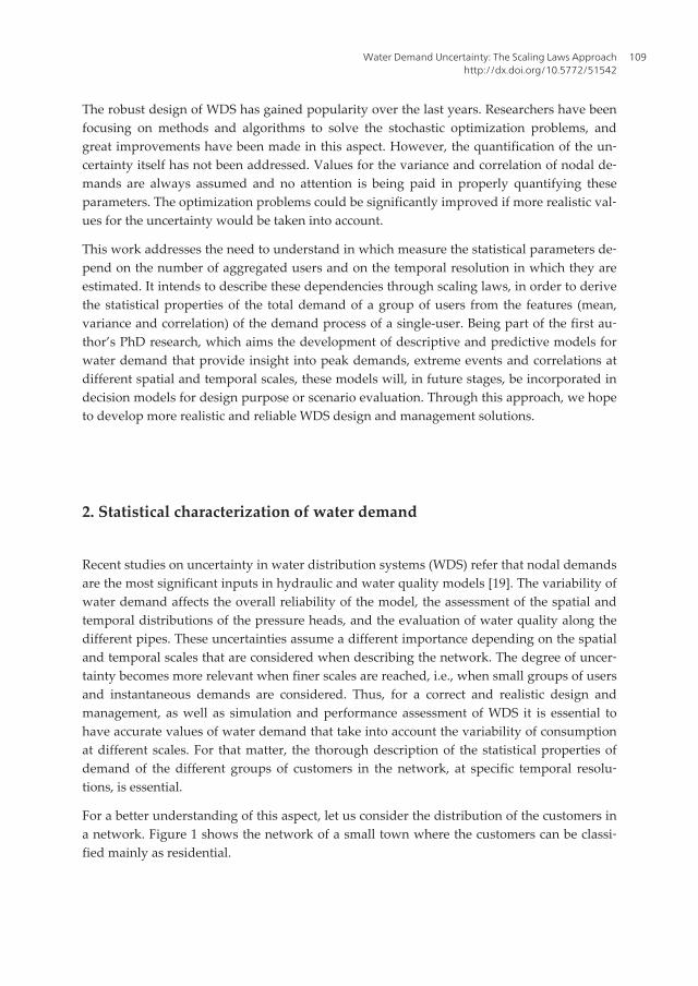
For a better understanding of this aspect, let us consider the distribution of the customers ina network. Figure 1 shows the network of a small town where the customers can be classi‐fied mainly as residential.


109

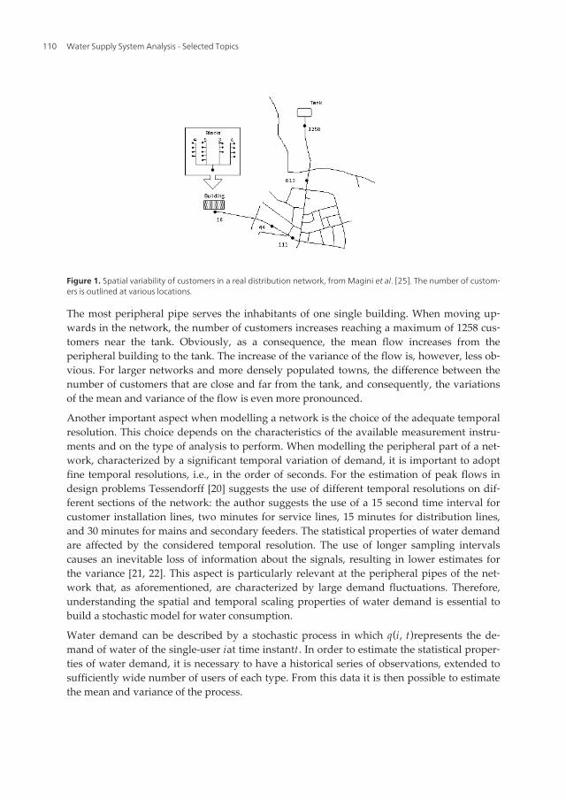
Figure 1. Spatial variability of customers in a real distribution network, from Magini et al. [25]. The number of custom‐ers is outlined at various locations.

The most peripheral pipe serves the inhabitants of one single building. When moving up‐wards in the network, the number of customers increases reaching a maximum of 1258 cus‐tomers near the tank. Obviously, as a consequence, the mean flow increases from theperipheral building to the tank. The increase of the variance of the flow is, however, less ob‐vious. For larger networks and more densely populated towns, the difference between thenumber of customers that are close and far from the tank, and consequently, the variationsof the mean and variance of the flow is even more pronounced.

Another important aspect when modelling a network is the choice of the adequate temporalresolution. This choice depends on the characteristics of the available measurement instru‐ments and on the type of analysis to perform. When modelling the peripheral part of a net‐work, characterized by a significant temporal variation of demand, it is important to adoptfine temporal resolutions, i.e., in the order of seconds. For the estimation of peak flows indesign problems Tessendorff [20] suggests the use of different temporal resolutions on dif‐ferent sections of the network: the author suggests the use of a 15 second time interval forcustomer installation lines, two minutes for service lines, 15 minutes for distribution lines,and 30 minutes for mains and secondary feeders. The statistical properties of water demandare affected by the considered temporal resolution. The use of longer sampling intervalscauses an inevitable loss of information about the signals, resulting in lower estimates forthe variance [21, 22]. This aspect is particularly relevant at the peripheral pipes of the net‐work that, as aforementioned, are characterized by large demand fluctuations. Therefore,understanding the spatial and temporal scaling properties of water demand is essential tobuild a stochastic model for water consumption.

Water demand can be described by a stochastic process in which q(i, t)represents the de‐mand of water of the single-user iat time instantt . In order to estimate the statistical proper‐ties of water demand, it is necessary to have a historical series of observations, extended tosufficiently wide number of users of each type. From this data it is then possible to estimatethe mean and variance of the process.


If the consumers are assumed to be of the same type, the properties of demand can be con‐sidered to be homogeneous in space, this is, they are independent of the particular consum‐er that is taken into consideration. Regarding the temporal variability, the stochastic processcan only be assumed to be stationary in time intervals during which the mean stays con‐stant. Once the length of this time interval, T , is established, it is possible to determine thetemporal mean, μ1, and variance,σ1

2 , of the demand signal of the single-useri, as followed:

μ1 = 1T ∫0

T q(i, t)dt (1)

σ12 = 1

T ∫0T q(i, t) - μ1

2dt (2)

For homogeneous and stationary demands, the expected values for the mean and variance,E μ1 andE σ1

2 , obtained from N observations, provide the mean and variance of the process.

2.1. Correlation between consumers

The definition of the mean and variance for each type of consumer is not enough for a com‐plete statistical characterization of demand. In order to obtain a realistic representation ofthe demand loads at the different nodes in a network; essential for the assessment of the net‐work performance under conditions as close as possible to the actual working conditions,the correlation between nodal demands cannot be ignored. This correlation can be expressedthrough the cross-covariance and cross-correlation coefficient functions.

The cross-covariance,covAB , and cross-correlation coefficient,ρAB , between user iof group Aand user jof groupB, during the observation periodT , are expressed, respectively, as fol‐lowed:

covAB = 1T ∫0

TqA(iA, t)−μA qB( jB, t)−μB dt (3)

ρAB =covAB

σA ⋅ σB(4)

As known, the WDS need to guarantee minimum working conditions, this is, the minimumpressure requirements have to be satisfied at each node even under maximum demandloading conditions. If all the consumers in the network are of the same type, it seems reason‐able to assume a perfect correlation between demands, and to simplify the analysis of thenetwork by assigning the same demand pattern to all the consumers. The synchronism ofdemands is the worst scenario that can occur on a network, causing the widest pressurefluctuations at the nodes. The assumption of a perfect correlation for design purposes resultsin reliable networks, but it also requires the increase of the pipe diameters, which conse‐quently increases the networks cost. In fact, as mentioned earlier, each consumer has his


111

own demand pattern based on specific needs and habits, without knowing what other con‐sumers are doing at the same time. This means that demand signals in real networks are cor‐related, but are not synchronous. Thus, in order to obtain the optimum design of a network,it is essential to estimate the accurate level of correlation between the consumers. On theother hand, to estimate accurately the spatial correlation between demands, it is necessary tocollect and analyse historical series, resulting in additional costs in the design phase. How‐ever, these additional costs will most certainly be compensated by the achieved reduction ofthe following construction costs.

2.2. The scaling laws approach in modelling water demand uncertainty

Water demand uncertainty is made of both aleatory or inherent uncertainty, due to the natu‐ral and unpredictable variability of demand in space and time, and epistemic or internal un‐certainty, due to a lack of knowledge about it. Hutton [23] distinguishes epistemicuncertainty in two types. The first type concerns the nature of the demand patterns, and thelack of knowledge about this variability when modelling WDS both in time and space. Thisuncertainty is defined as ‘two-dimensional’ uncertainty since it is composed by both aleato‐ry and epistemic uncertainty. It can be reduced with extended and expensive spatial andtemporal data collection or through the employment of descriptive and predictive water de‐mand models. The second type of epistemic uncertainty takes the spatial allocation of waterdemand into account when modelling WDS [24].

Dealing with the ’two-dimensional’ uncertainty when modelling WDS, requires not only acomplete statistical characterization of demand variability, but also the determination of thecorrelation among the different users and groups of users. The natural variability of demandcan be expressed using probability density functions (PDF). A PDF is characterized by itsshape (e.g. normal, exponential, gamma, among others) and by specific parameters like thepopulation mean and variance. Thus, in order to represent uncertain water demand using aPDF, it is necessary to identify and estimate the values of these parameters. The considera‐tion of different spatial and temporal aggregation levels induces changes in the PDF param‐eters, often leading to a reduction of the uncertainty. The auto-correlation and cross-correlation that characterize the water demand signals affect the extent to which the PDFparameters vary, and can introduce an additional sensitivity to the specific period of obser‐vation in question.

In order to understand the effects of spatial aggregation and sampling intervals on the statis‐tical properties of demand, it is possible to develop analytical expressions for the moments(mean, variance, cross-covariance and cross-correlation coefficient) of demand time series, ata fixed time sampling frequency∆ t , of naggregated users as a function of the moments ofthe single-user series sampled in the observation period T. These expressions are referred toas “Scaling Laws”, and can be expressed as:

E m∆t ,T (n) = E m∆t ,T ⋅n α ⋅ f (∆ t , T ) (5)


WhereE m∆t ,T (n) is the expected value of the moment mfor nusers for the time intervalT ;E m∆t ,T is the expected value of the moment mfor the single-user for the same time interval;αis the exponent of the scaling law; and f (∆ t , T )is a function that expresses the influence ofboth sampling rate and observation period.

The development of the scaling laws is based on the assumption that the demand can be de‐scribed by a homogeneous and stationary process, which implies that the naggregated usersare of the same type (residential, commercial, industrial, etc.), and that the statistical proper‐ties of demand, mean and variance, can be assumed constant in time. The scaling laws forthe mean, variance, and lag1 covariance were derived by Magini [25]. The expected value ofthe total mean demand q(n, t)can be expressed as followed:

E μ∆t ,T (n) = E 1T ∫0

T ∑j=1

nq( j, τ)dτ = 1

T ∫0T ∑

j=1

nE q( j, τ) dτ =n ⋅E μ1 (6)

Where E μ1 is the expected demand value for the single user or ‘unit mean’. This expres‐sion shows that the mean demand increases linearly with the number of users according to afactor of proportionality equal to the expected value of the single user and is independent ofthe sampling rate and observation period.

In order to estimate the expected value of the demand variance it is necessary to considerthe covariance function cov(s, τ)of the single-user demand at the spatial and temporal lags,s = j1 - j2andτ =τ1 - τ2, respectively. The following expression is obtained (see [26] for themathematical passages):

E σΔt ,T2 (n) =

1T 2 ∫0

T ∫0T∑i1=1

n∑i2=1

ncovΔt(s,0)−covΔt(s, τ) dτ1dτ2

=∑i1=1

n∑i2=1

ncovΔt(s,0)−

1T 2 ∫0

T ∫0T

covΔt(s, τ)dτ1dτ2

(7)

Where cov∆t(s, 0) is the covariance function at lags =0, and cov∆t(s, τ) is the space-time cova‐riance function. This expression shows that the expected value for the sample variance ofthe n-users process depends on the correlation structure of the single-user demands. The

term 1T 2 ∫0

T ∫0T cov∆t(s, τ)dτ1dτ2 decreases as the period of observation T increases, becoming

negligible whenT > >θ, being θ a parameter, connected to the cross-correlation of the de‐mands and similar to the scale of fluctuation for the auto-correlation of a single signal.

The term cov∆t(s, 0) is independent from τ1 andτ2, and assumes the following values:

covΔt(s,0)= {covΔt(s) j1≠ j2σ1,Δt

2 j1 = j2(8)


113

Where cov∆t(s) is the spatial cross-covariance between different single-user demands, and

σ1,∆t2 the variance of the single user. For large values ofT , equation (7) can be simplified into:

E σΔt ,T2 (n) =∑

j1=1

n∑j2=1

ncovΔt(s,0)=∑

j1=1

n∑j2= j1

covΔt(s,0) + ∑j1=1

n∑j2≠ j1

covΔt(s,0)

=n ⋅σ1,Δt2 + n ⋅ (n −1)⋅ covΔt(s)

(9)

This equation represents the scaling law for the variance, neglecting the bias that can becaused when using small the demand series (short observation periods).

Introducing the Pearson cross-correlation coefficient given byρ =cov xy

σxσy, and considering ρΔt

as the cross-correlation coefficient between each couple of single-user demands, the spatialcovariance can be expressed ascovΔt =ρΔT σ1,Δt

2 , and Equation (9) becomes:

E σ∆t2 (n) =n 2⋅ρ∆t ⋅σ1,∆t

2 + n ⋅ 1 - ρ∆t ⋅σ1,∆t2 (10)

If demands are perfectly correlated in space then ρ∆t is equal to one, and equation (10) issimplified into:

E σ∆t2 (n) =n 2⋅σ1,∆t

2 (11)

If demands are uncorrelated in space then ρΔtis equal to zero, and equation (9) is simplifiedinto:

E σ∆t2 (n) =n ⋅σ1,∆t

2 (12)

Since the cross-correlation coefficient can assume values between 0 and1, equations (10) and(11) represent the maximum and minimum expected values for the variance. Equation (9)can be simplified into a more generic form given by:

E σ∆t2 (n) =n α ⋅σ1,∆t

2 (13)

Where1≤α ≤2.

In conclusion, it can be stated that the variance in the consumption signal of a group of usersn, homogeneous in type, is proportional to the mean variance of the single-user according toan exponent, which varies between 1 and 2. The value of the scaling exponent depends onthe structure of the spatial correlation, i.e., the correlation that exists between the differentconsumptions during the observation period: if demands are uncorrelated in space, the scal‐ing law is linear, if demands are perfectly correlated in space, the scaling law is quadratic.


The variance function, γ(Δt), measures the reduction of the variance of the instantaneoussignal when the sampling interval Δtincreases [27], as followed:

σ1,∆t2 =σ1

2⋅γ(Δt) (14)

Where σ12 is the variance of the instantaneous signal for the single user. Introducing the var‐

iance function in equation (13), the following is obtained:

E σ∆t2 (n) =n α ⋅σ1

2⋅φ(∆ t) (15)

Similarly, the expected value of the cross-covariance is given by:

E covAB,Δt(na, nb) = 1T 2 ∫0

T ∫0T∑i=1

na

∑j=1

nb

covAB,Δt(s,0)−covAB,Δt(s, τ) dτ1dτ2

=∑i=1

n∑j=1

ncovAB,Δt(s,0)−

1T 2 ∫0

T ∫0T

covAB,Δt(s, τ)dτ1dτ2

(16)

Neglecting the term 1T 2 ∫0

T ∫0T cov AB,∆t(s, τ)dτ1dτ2, the expected value of the cross-covariance

between the demands of na aggregated users of group A and nb aggregated users of group B

is given by:

E cov AB,∆t(na, nb) =na ⋅nb ⋅E ρab,∆t ⋅E σa,∆t ⋅E σb,∆t (17)

Where, E ρab,∆t is the expected Pearson cross-correlation coefficient between the single-user

demands of the two groups; and σa,∆t and σb,∆tare the standard deviations of the single-user

demands of groups AandB, respectively, at the sampling rate∆ t . The expected value of thecross-covariance increases according to the product between the number of users of eachgroup. In the particular case in which both groups have the same statistical properties, i.e.,they belong to the same process, and assuming thatna =nb, the scaling law of the cross-cova‐

riance becomes quadratic.

As a consequence, the expected value of the Pearson cross-correlation coefficient betweenthe demands of na aggregated users of group A and nb aggregated users of group B, is given

by:

E ρAB,∆t(na, nb) =E Cov AB ,∆t (na, nb)

E σA,∆t (na) ⋅ E σB ,∆t (nb)=

na ⋅ nb ⋅ E ρab,∆t

na(1 + E ρa,∆t ⋅ na - 1 ) ⋅ nb(1 + E ρb,∆t ⋅ nb - 1 ) (18)


115

This equation shows that this coefficient depends separately on the spatial aggregation lev‐els of each group, na and nb, and not only on their product as happens for the cross-cova‐riance. If na = nb = n equation [18] becomes:

E ρAB,∆t(n) =n ⋅ E ρab,∆t

1 + (n - 1) ⋅ E ρa,∆t 1 + (n - 1) ⋅ E ρb,∆t

(19)

From equation (19) it is possible to observe that the expected value E ρAB,∆t(na, nb) increaseswith the number of users, naandnb, reaching the following limit value:

E ρAB,Δt(na, nb) = limna→∞

nb→∞

E ρAB,Δt(na, nb) =E ρab,Δt

(E ρa,Δt ⋅ E ρb,Δt ) (20)

Since by definitionE ρab,Δt ≤1, the maximum value that the expected value of the cross-cor‐relation coefficient between the single-user demands of group Aand Bcan assume is:

E ρAB,∆t max = (E ρa,∆t ⋅E ρb,∆t ) (21)

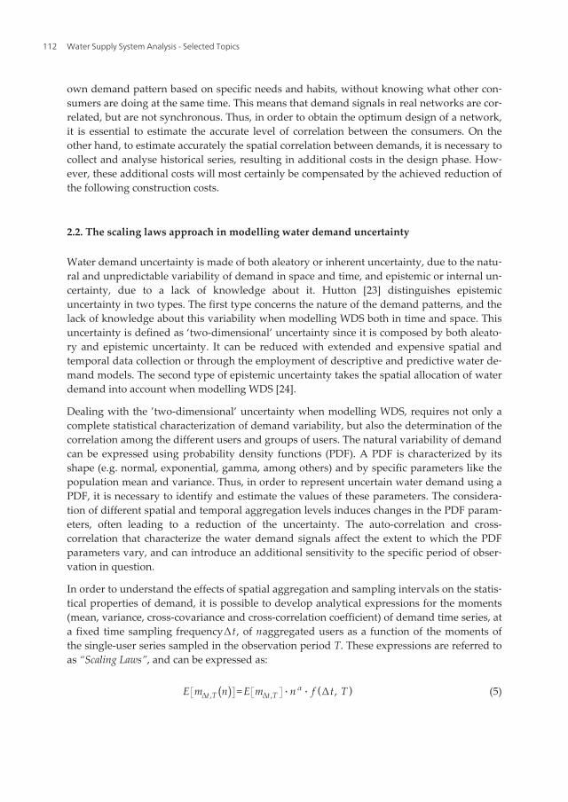
From equation (21) it is also possible to observe that the Pearson cross-correlation coefficientbetween the na aggregated users of group Aand the nb aggregated users of group Bdependson both the cross-correlations inside each group and the cross-correlation between thegroups. Therefore, it seems interesting to investigate the way in which these two aspects,one at a time, affect the expected value of the cross-correlation when the number of aggre‐gated users increases and for a fixed sampling rate∆ t . In order to do so let us first consider afixed value of ρab and varying values of ρa andρb. Figure 2 shows the graphical results forρab =0.1 and different pairs of ρa andρb.

As expected, all the curves have a common starting point, since ρab is fixed. According toequation (19) a gradual flattening of the curves and a reduction of the shape ratio ρAB,lim / ρab

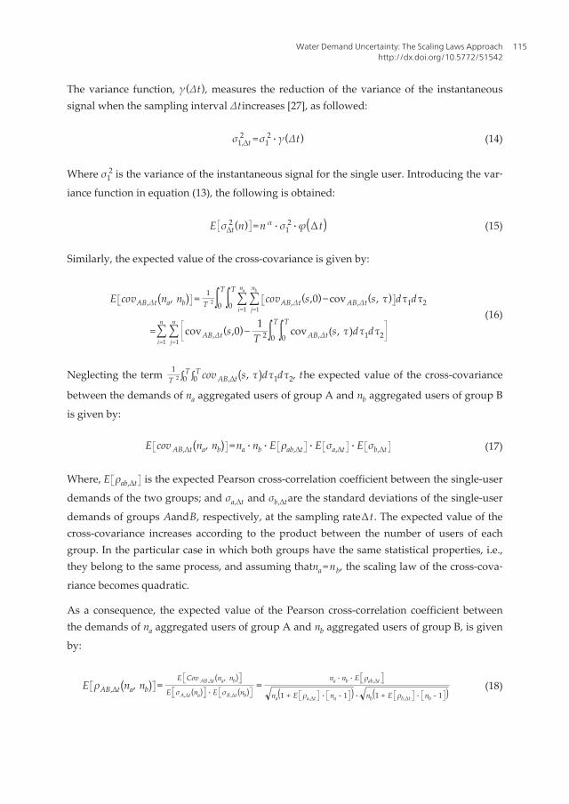
can be noticed when the product ρa ⋅ρb increases. Let us now consider a different case inwhich ρa and ρb are fixed and ρabvaries. The results are shown graphically in figure 3. Thecurves have now different starting points and equal shape ratiosρAB,lim / ρab. Increasing ρab

produces only an upward shift of the curves, extending their transient.


Figure 2. Scaling laws ofE ρAB(n) , for different values ofρa ⋅ρb.

Figure 3. Scaling laws ofE ρAB(n) , for different values ofρab.

In the particular case in which both groups of users have the same statistical properties, i.e.,they belong to the same process, and assumingna =nb =n, the scaling law for the cross-corre‐lation coefficient, considering no differences in the sampling time intervals, is:

E ρAB,∆t(n) =n ⋅ E ρ∆t

1 + (n - 1) ⋅ E ρ∆t

(22)

From equation (22) it is clear that the cross-correlation coefficientincreases with the numberof aggregated users, tending to one. This limit value is reached as sooner as the cross-corre‐lation coefficient, E ρ∆t , between the single-user demands is higher.


117

3. Validation of the Analytical expressions

3.1. Synthetically generated signals: scaling laws for the mean and the variance

In order to confirm the analytical development reported in the previous paragraph, the scal‐ing laws were derived for groups of synthetically and simultaneously generated consump‐tion signals. At this aim the Multivariate Streamflow model [28], with a normal probabilitydistribution, was used. Each group was assumed to contain 300 consumption signals with3600 realizations each, distinguished by different values of the cross-correlation coefficientbetween them. The correctness of the procedure used to generate each demand series wastested by checking that the mean, the variance and the cross-correlation coefficient of thegenerated signals were equal to the input parameters of the model. Only little differenceswere observed (Table 1), which are explained due to the fact that the generated demand ser‐ies are realizations of a stochastic process and, consequently, their moments necessarily dif‐fer from the theoretical ones.

Once the single consumption signals of each group were generated, they were aggregatedrandomly selecting one at a time, until a maximum of 100 aggregated consumption signalswas reached. The first and second order moments, mean and variance, were calculated foreach aggregation level. In order to obtain a result as general as possible, the same procedurehas been repeated 50 times, aggregating each time different users [25]. The obtained resultsare summarized in Table 1 and 2, with reference to equation 5.

Cross-correlation

coefficient

E[mT] α

Theoretical Experimental Theoretical Experimental

0 0.70 0.7003 1.00 0.9996

0.001 0.70 0.7017 1.00 0.9993

0.010 0.70 0.6971 1.00 1.0001

0.025 0.70 0.7020 1.00 0.9989

0.050 0.70 0.7096 1.00 1.0004

0.10 0.70 0.7063 1.00 1.0009

0.20 0.70 0.7086 1.00 0.9994

0.30 0.70 0.7032 1.00 1.0008

0.40 0.70 0.6923 1.00 1.0003

0.50 0.70 0.6942 1.00 0.9985

0.60 0.70 0.6857 1.00 1.0002

0.70 0.70 0.6874 1.00 1.0011

0.80 0.70 0.6852 1.00 0.9998

0.90 0.70 0.6789 1.00 1.0009

0.99 0.70 0.7050 1.00 0.9997

Table 1. Theoretical and experimental values of the scaling law for the first order moment for different values of thecross-correlation.


Cross-correlation

coefficientE[mT] α

0 3.9808 1.0004

0.001 3.5205 1.0541

0.010 1.9864 1.3079

0.025 1.4498 1.4984

0.050 1.2702 1.6403

0.10 1.2940 1.7686

0.20 1.5621 1.8675

0.30 1.8879 1.9139

0.40 2.1713 1.9379

0.50 2.4485 1.9570

0.60 2.7685 1.9692

0.70 3.0803 1.9804

0.80 3.4051 1.9888

0.90 3.6567 1.9945

0.99 3.9960 1.9985

Table 2. Experimental values of the scaling law for the second order moment for different values of the cross-correlation.

Results confirm the linear scaling for the first order moment and show that the variance in‐creases with the spatial aggregation level according to an exponent that varies between 1and 2. In theory, for spatially uncorrelated demands the scaling laws is linear and for per‐fectly correlated demands the scaling law is quadratic.

3.2. Synthetically generated signals: scaling laws for the cross-covariance

In this case pairs of aggregated consumption series, A and B, were obtained by randomlyselecting among pairs of the previously generated groups of signals. Different values of theproductna ⋅nb, where na is the number of signals in group A and nb the same number ingroup B, were considered, up to the maximum valuena ⋅nb =500. Each aggregation processwas characterized by the cross-correlation value between the single signals in the samegroup and the cross-correlation value between the single signals of the two native groups.The cross-covariance was computed for the different aggregation levels and the scaling lawwere derived for each process. The results are summarized in Table 3 with reference toequation 17, considering Coeff = E ρab,ΔT ⋅E σa,ΔT ⋅E σb,ΔT and α as the exponent of theproduct na ⋅nb.


119

Cross-correlation coefficient Coeff α

ρa ρb ρab theoretical experimental theoretical experimental

0.10 0.10 0.10 0.3754 0.3747 1.00 0.9998

0.20 0.10 0.10 0.3880 0.3907 1.00 0.9982

0.40 0.10 0.10 0.3676 0.3624 1.00 1.0020

0.40 0.20 0.10 0.3463 0.3440 1.00 1.0003

0.80 0.60 0.10 0.3939 0.3908 1.00 1.0009

0.50 0.50 0.10 0.3545 0.3541 1.00 0.9993

0.50 0.50 0.20 0.7449 0.7401 1.00 1.0007

0.50 0.50 0.30 1.0999 1.0923 1.00 1.0004

0.50 0.50 0.40 1.4643 1.4605 1.00 0.9999

0.50 0.50 0.50 1.8408 1.8504 1.00 0.9986

Table 3. Theoretical and experimental values of the scaling law for the cross-covariance for different values of thecross-correlation coefficients in, ρa and ρb, and between A,B, ρab.

Results confirm that α is always equal to one. However, in this case the scaling does not con‐

sider the number of aggregated users, but their product, and thus the law is not linear but

quadratic. A similar approach was also applied in the particular case in whichρa =ρb =ρab,

andσa =σb, that is, when all the consumptions are homogeneous, and withna =nb.

Cross-correlation Coeff α

coefficient theoretical experimental theoretical experimental

0.10 0.40 0.4000 2.00 1.9998

0.20 0.80 0.7914 2.00 1.9997

0.30 1.20 1.2160 2.00 2.0008

0.40 1.60 1.6009 2.00 1.9985

0.50 2.00 2.0059 2.00 1.9992

0.60 2.40 2.3955 2.00 2.0003

0.70 2.80 2.7934 2.00 2.0000

0.80 3.20 3.2043 2.00 1.9999

0.90 3.60 3.6057 2.00 1.9999

0.99 3.96 3.9408 2.00 2.0003

Table 4. Theoretical and experimental values of the scaling law for the cross-covariance between homogeneousgroups of consumptions and different values of the cross-correlation coefficient.


Equation 17 then becomes E cov AB,T (na, nb) =n 2⋅E ρab,∆t ⋅E σ∆t2 .The results for different

values of the cross-correlation coefficient are described in Table 4. They confirm the theoreti‐cal quadratic scaling for cross-covariance.

3.3. Real consumption data: scaling laws for the mean and the variance

The parameters of the scaling laws were also derived for a set of real demand data. The in‐door water uses demand series of 82 single-family homes, with a total of 177 inhabitants, ina building belonging to the IIACP (Italian Association of Council Houses) in the town ofLatina were considered [29, 30]. The apartments are inhabited by single-income families, be‐longing to the same low socioeconomic class.The daily demand series of four different days(4 consecutive Mondays) of the 82 users were considered [25]. For each user the differentdays of consumptions can be considered different realizations of the same stochastic proc‐ess. In this way the number of customers was artificially extended to about 300, preservingat the same time the homogeneity of the sample. The temporal resolution of each time seriesis 1 second.

TimeE [μ1] E [σ2 1] αvar

(L/min) (L /min)2 -

6-7 0.468 1.994 1.2288

7-8 1.066 6.678 1.114

8-9 0.988 7.401 1.0435

9-10 0.891 6.205 1.0756

10-11 0.735 4.336 1.113

11-12 0.791 4.782 1.089

12-13 0.68 4.452 1.092

13-14 0.807 5.322 1.065

14-15 0.827 5.338 1.0688

15-16 0.704 3.857 1.1311

16-17 0.512 2.266 1.1739

17-18 0.634 3.112 1.1666

18-19 0.667 3.594 1.1412

19-20 0.707 5.445 1.0384

20-21 0.68 3.702 1.1253

21-22 0.635 3.412 1.099

22-23 0.397 1.958 1.0771

mean 0.717 4.344 1.1084

confidence limits 95% 0.082 0.759 0.024

Table 5. Estimated parameters of the scaling laws for the experimental data set of Latina (see [25]).


121

The series were divided into time periods of 1 hour to guarantee the stationarity of the proc‐ess. In Table 5 the estimated values of the expected values of the mean and the variance ofthe unit user and the exponent α for the scaling law of the variance are reported. The sameexponents for the mean were always trivially equal to 1. In these results the first six hoursof the day and the last one were excluded because, during the night hours consumptionsare very small and therefore their statistics have a poor significance. It was observed thatthe mean scales linearly with the number of customers. Differently, the variance shows aslight non-linearity with the number of users. It must be underlined that the average dai‐ly value of the exponent α is 1.1, showing that there is a very weak correlation betweenthe considered users.

3.4. Real consumption data: scaling laws for the cross-covariance andcross-correlationcoefficient

Considering the consumption signals belonging to homogeneous users, equation 23 is validand a quadratic scaling law for the cross-covariance should be expected. This behaviour wasconfirmed by the measured data for all the time intervals considered. In Figure 4 the scalinglaw of the consumption signals between 11:00 and 12:00 am is graphically reported.

Figure 4. Scaling law for the cross-covariance between 11:00 and 12:00am.

The obtained cross-correlation coefficient between the single user signals was low, being al‐ways less than 0.05, but increased noticeably when the number of aggregated users in‐creased, as expected according to equation 22. For groups of 150 aggregated users the cross-correlation coefficient reached the values shown in Table 6. These results enhance theimportance of evaluating the cross-correlation degree at different levels of spatial aggrega‐tion. Even if the cross-correlation between single-user demand signals is relatively low andless likely to significantly affect the performance of a network, it can largely increase withthe spatial aggregation of users, becoming not negligible at those larger scales.


Time ρ150users Time ρ150users

0-1 0.56 13-14 0.49

1-2 0.6 14-15 0.5

3-4 0.5 15-16 0.42

4-5 0.58 16-17 0.49

5-6 0.36 17-18 0.5

6-7 0.48 18-19 0.39

7-8 0.71 19-20 0.51

8-9 0.61 20-21 0.52

9-10 0.39 21-22 0.39

10-11 0.46 22-23 0.47

11-12 0.57 23-24 0.61

12-13 0.48 - -

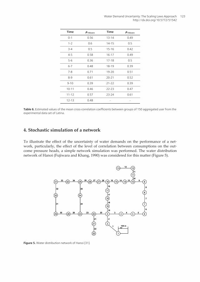
Table 6. Estimated values of the mean cross-correlation coefficients between groups of 150 aggregated user from theexperimental data set of Latina.

4. Stochastic simulation of a network

To illustrate the effect of the uncertainty of water demands on the performance of a net‐work, particularly, the effect of the level of correlation between consumptions on the out‐come pressure heads, a simple network simulation was performed. The water distributionnetwork of Hanoi (Fujiwara and Khang, 1990) was considered for this matter (Figure 5).

Figure 5. Water distribution network of Hanoi [31].


123

The data for the Hanoi network were taken from the literature (Fujiwara and Khang, 1990),and the pipe diameters were assumed to be the ones obtained by Cunha and Sousa (2001).The demand data from the literature was used to estimate the number of users at each node,assuming a single-user mean demand of 0.002 l/s. All the users in the network were as‐sumed to be residential and having the same characteristics. The standard deviation of de‐mand was assumed to be 0.06 l/s. The Multivariate Streamflow model [28] was used togenerate synthetic stochastic demands with different levels of cross-correlation between thesingle-users. The nodal demands were then introduced in the network and the performanceof the network was simulated using EPANET [32]. For each considered degree of cross-cor‐relation between demands, 100 simulations were performed, resulting in series of pressureheads for each node and for each correlation level.

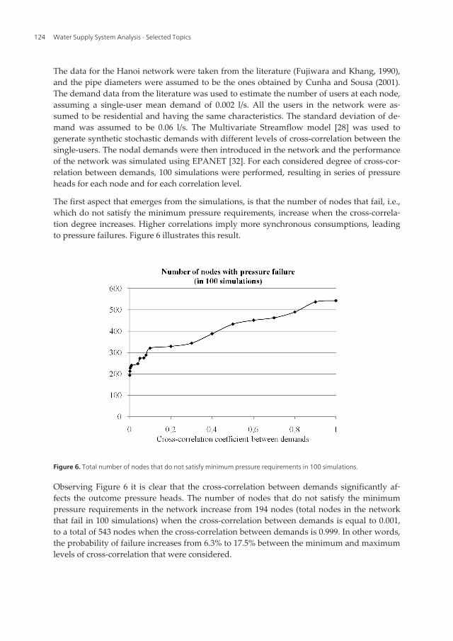
The first aspect that emerges from the simulations, is that the number of nodes that fail, i.e.,which do not satisfy the minimum pressure requirements, increase when the cross-correla‐tion degree increases. Higher correlations imply more synchronous consumptions, leadingto pressure failures. Figure 6 illustrates this result.

Figure 6. Total number of nodes that do not satisfy minimum pressure requirements in 100 simulations.

Observing Figure 6 it is clear that the cross-correlation between demands significantly af‐fects the outcome pressure heads. The number of nodes that do not satisfy the minimumpressure requirements in the network increase from 194 nodes (total nodes in the networkthat fail in 100 simulations) when the cross-correlation between demands is equal to 0.001,to a total of 543 nodes when the cross-correlation between demands is 0.999. In other words,the probability of failure increases from 6.3% to 17.5% between the minimum and maximumlevels of cross-correlation that were considered.


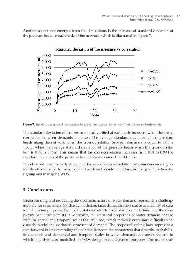
Another aspect that emerges from the simulations is the increase of standard deviation ofthe pressure heads at each node of the network, which is illustrated in Figure 7.

Figure 7. Standard deviation of the pressure heads vs the cross-correlation coefficient between the demands.

The standard deviation of the pressure head verified at each node increases when the cross-correlation between demands increases. The average standard deviation of the pressureheads along the network when the cross-correlation between demands is equal to 0.01 is1.35m, while the average standard deviation of the pressure heads when the cross-correla‐tion is 0.99, is 5.75m. This means that the cross-correlation increases from 0.01 to 0.99 thestandard deviation of the pressure heads increases more than 4 times.

The obtained results clearly show that the level of cross-correlation between demands signif‐icantly affects the performance of a network and should, therefore, not be ignored when de‐signing and managing WDS.

5. Conclusions

Understanding and modelling the stochastic nature of water demand represents a challeng‐ing field for researchers. Stochastic modelling faces difficulties like scarce availability of datafor calibration purposes, high computational efforts associated to simulations, and the com‐plexity of the problem itself. Moreover, the statistical properties of water demand changewith the spatial and temporal scales that are used, which makes it even more difficult to ac‐curately model the stochastic structure of demand. The proposed scaling laws represent astep forward in understanding the relation between the parameters that describe probabilis‐tic demands and the spatial and temporal scales in which demands are measured and inwhich they should be modelled for WDS design or management purposes. The use of scal‐


125

ing laws allow a more accurate quantification of the statistical parameters, like variance andcorrelation, based on the real demand patterns, number of users at each node and the sam‐pling time that is used. The scaling laws also allow to easily change the scale of the problem,since the statistical parameters and levels of uncertainty can be derived for any desired timeor spatial scale.

The scaling laws were derived analytically and validated using synthetically generated sto‐chastic demands and real demand data from Latina, Italy. A good agreement was found be‐tween the theoretical expressions, the synthetic demand data and the real demand data.Results show that the mean increases linearly with the number of aggregated users. The var‐iance increases with spatial aggregation according to an exponent that varies between 1 and2. In theory, for spatially uncorrelated demands the scaling laws is linear and for perfectlycorrelated demands the scaling law is quadratic. This aspect is clearly verified by the syn‐thetic data. The scaling law for the covariance between 2 groups of users increases accordingto the product between the numbers of users in each group. The cross-correlation coefficientdepends separately on the number of users in each group, and increases towards a limit val‐ue. Even for small values of cross-correlation between single-user demands, this parametercannot be ignored since it significantly increases with the aggregation of consumers.

The performed network simulation considering stochastic demands with different pre-de‐fined levels of correlation show a clear influence of the degree of correlation on the outcomepressure heads: higher levels of correlation lead to larger fluctuations of the pressure headsand to more frequent pressure failures. At this point, the stochastic correlated demandswere only used for simulation purposes. However, in future work a similar approach, canbe used for design and management purposes. The consideration of correlated stochastic de‐mands will result in more realistic and reliable water distribution networks.

Acknowledgements

The participation of the first author in the study has been supported by Fundação para aCiência e Tecnologia through Grant SFRH/BD/65842/2009.

Author details

Ina Vertommen1,2, Roberto Magini2*, Maria da Conceição Cunha1 and Roberto Guercio2

*Address all correspondence to: [email protected]

1 Department of Civil Engineering, University of Coimbra, Coimbra, Portugal

2 Department of Civil, Building and Environmental Engineering, La Sapienza University ofRome, Rome, Italy


References

[1] Buchberger, S. G., & Wu, L. (1995). Model for instantaneous residential water de‐mands. Journal of Hydraulic Engineering, ASCE, 121(3), 232-246.

[2] Buchberger, S. G., & Wells, G. J. (1996). Intensity, Duration, and Frequency of Resi‐dential Water Demands. Journal of Water Resources Planning and Management, ASCE,122(1), 11-19.

[3] Garcia, V. J., Garcia-Bartual, R., Cabrera, E., Arregui, F., & Garcia-Serra, J. (2004). Sto‐chastic Model to Evaluate Residential Water Demands. Water Resources Planning andManagement, ASCE, 130(5), 386-394.

[4] Buchberger, S. G., & Lee, Y.. (1999). Evidence supporting the Poisson pulse hypothe‐sis for residential water demands. Water Industry systems: Modelling and optimizationapplications, 215-227.

[5] Alvisi, S., Franchini, M., & Marinelli, A. (2003). A stochastic model for representingdrinking water demand at resindential level. Water Resources Management, 17,197-222.

[6] Blokker, E. J. M., & Vreeburg, J. H. G. (2005). Monte Carlo Simulation of ResidentialWater Demand: A Stochastic End-Use Model. Impacts of Global Climate Change, 2005World Water and Environmental Resources Congress, Anchorage, Alaska: American So‐ciety of Civil Engineers.

[7] Blokker, E. J. M., Vreeburg, J. H. G., & Vogelaar, A. J. (2006). Combining the probabil‐istic demand model SIMDEUM with a network model Water Distribution SystemAnalysis. 8th Annual Water Distribution Systems Analysis Symposium , Cincinnati,Ohio, USA.

[8] Blokker, E. J. M., Buchberger, S. G., Vreeburg, J. H. G., & van Dijk, J. C. (2008). Com‐parison of water demand models: PRP and SIMDEUM applied to Milford, Ohio, da‐ta. WDSA, Kruger Park, South Africa.

[9] Buchberger, S. G., Blokker, E. J. M., & Vreeburg, J. H. G. (2008). Sizes for Self-Clean‐ing Pipes in Municipal Water Supply Systems. WDSA, Kruger Park, South Africa.

[10] Li, Z., Buchberger, S. G., Boccelli, D., & Filion, Y. (2007). Spatial correlation analysisof stochastic residential water demands. Water Management Chalenges in GlobalChange, London: Taylor & Francis Group.

[11] Blokker, E. J. M., Vreeburg, J. H. G., & van Dijk, J. C. (2010). Simulating ResidentialWater Demand with a Stochastic End-Use Model. Journal of Water Resources Planningand Management, ASCE, 136(1), 19-26.

[12] Moughton, L. J., Buchberger, S. G., Boccelli, D. L., Filion, Y., & Karney, B. W. (2006).Effect of time step and data aggregation on cross correlation of residential demands, Cincin‐nati, Ohio, USA.


127

[13] Lansey, K. E., & Mays, L. W. (1989). Optimization model for water distribution sys‐tem design. Journal of Hydraulic Engineering, ASCE, 115, 10, 1401-1418.

[14] Xu, C., & Goulter, I. C. (1998). Probabilistic model for water distribution reliability.Journal of Water Resources Planning and Management, ASCE, 124(4), 218-228.

[15] Kapelan, Z., Babayan, A. V., Savic, D., Walters, G. A., & Khu, S. T. (2004). Two newapproaches for the stochastic least cost design of water distribution systems. 4thWorld Water Congress: Innovation in Drinking Water Treatmen, London.

[16] Babayan, A., Savic, D., & Walters, G. (2005). Multiobjective optimization of water distri‐bution system design under uncertain demand and pipe roughness, School of Engineering,Computer Science and Mathematics, University of Exeter: Exeter.

[17] Kapelan, Z., Savic, D., & Walters, G. (2005). An Efficient Sampling-based Approach forthe Robust Rehabilitation of Water Distribution Systems under Correlated Nodal Demands,School of Engineering, Computer Science and Mathematics, University of Exeter: Ex‐eter.

[18] Filion, Y., Adams, B., & Karney, A. (2007). Cross Correlation of Demands in WaterDistribution Network Design. Water Resources Planning and Management, ASCE,137-144.

[19] Pasha, K. (2005). Analysis of uncertainty on water distribution hydraulics and waterquality. Impacts of Global Climate Change, Anchorage, Alaska.

[20] Tessendorff, H. (1972). Problems of peak demands and remedial measures. Proc., 9thCong. Int. Water Supply Assoc. int. standing committee on Distribution Problems: subject n.2.

[21] Rodriguez-Iturbe, I., Gupta, V. K., & Waymire, E. (1984). Scale considerations in themodeling of temporal rainfall. Water Resources Research, 20(11), 1611-1619.

[22] Buchberger, S. G., & Nadimpalli, G. (2004). Leak estimation in water distribution sys‐tems by statistical analysis of flow reading. Water Resources Planning and Management,ASCE [130, 4], 321-329.

[23] Hutton, C. J., Vamvakeridou-Lyrouda, L. S., Kapelan, Z., & Savic, D. (2011). Uncer‐tainty Quantification and Reduction in Urban Water Systems (UWS) Modelling:Evaluation report.

[24] Giustolisi, O., & Todini, E. (2009). Pipe hydraulic resistance correction in WDN anal‐ysis. Urban Water Journal, 6(1), 39-52.

[25] Magini, R., Pallavicini, I., & Guercio, R. (2008). Spatial and temporal scaling proper‐ties of water demand. Journal of Water Resources Planning and Management, ASCE, 134,276-284.

[26] Rodriguez-Iturbe, I., Marani, M., D’Odorico, P., & Rinaldo, A. (1998). On space-timescaling of cumulated rainfall fields. Water Resources Research, 34(12), 3461-3469.


[27] Van Marcke, E. (1983). Random Fields Analysis and Synthesis (Revised and Expanded NewEdition), World Scientific Publishing Co. Pte. Ltd.

[28] Fiering, M. B. (1964). Multivariate Technique for Synthetic Hydrology. Journal of Hy‐draulics Division - Proceedings of the American Society of Civil Engineers, 43-60.

[29] Guercio, R., Magini, R., & Pallavicini, I. (2003). Temporal and spatial aggregation inmodeling residential water demand. Water Resources Management II, UK: WIT Press.

[30] Pallavicini, I., & Magini, R. (2007). Experimental analysis of residential water de‐mand data: probabilistic estimation of peak coefficients at small time scales. Proc.CCWI2007 & SUWM2007 Conf. Water Management Challenges in Global Change UK.

[31] Fujiwara, O., & Khang, D. B. (1990). A two phase decomposition method for optimaldesign of looped water distribution networks. Water Resources Research, 26(4),539-549.

[32] Rossman, L. A. (2000). Epanet2 Users Manual, Washington, USA: US EPA.


129

water demand uncertainty: the scaling laws approach

Documents