water evaluation and planning system tutorial - … evaluation and planning system tutorial overview...
TRANSCRIPT

WEAP Water Evaluation And Planning System
Tutorial
A collection of stand-alone modules to aid in learning the WEAP software
June 2005


WEAP Water Evaluation And Planning System
Tutorial Overview
Introduction ................................................................4
Background .................................................................4
WEAP Development...................................................5
The WEAP Approach .................................................5
Program Structure......................................................6
The Tutorial Structure..............................................11
June 2005

4 WEAP Tutorial
Introduction WEAP© is a microcomputer tool for integrated water resources planning. It provides a comprehensive, flexible and user‐friendly framework for policy analysis. A growing number of water professionals are finding WEAP to be a useful addition to their toolbox of models, databases, spreadsheets and other software.
This overview summarizes WEAP’s purpose, approach and structure. The contents of the WEAP tutorial are also introduced; the tutorial is constructed as a series of modules that takes you through all aspects of WEAP modeling capabilities. Although the tutorial itself is built on very simple examples, it covers most aspects of WEAP. A more complex model presenting those aspects in the context of a real situation is included with WEAP under the name “Weeping River Basin”. A detailed technical description is also available in a separate publication, the WEAP User Guide.
Background Many regions are facing formidable freshwater management challenges. Allocation of limited water resources, environmental quality, and policies for sustainable water use are issues of increasing concern. Conventional supply‐oriented simulation models are not always adequate. Over the last decade, an integrated approach to water development has emerged that places water supply projects in the context of demand‐side issues, water quality and ecosystem preservation.
WEAP aims to incorporate these values into a practical tool for water resources planning. WEAP is distinguished by its integrated approach to simulating water systems and by its policy orientation. WEAP places the demand side of the equation ‐ water use patterns, equipment efficiencies, re‐use, prices and allocation ‐ on an equal footing with the supply side ‐ streamflow, groundwater, reservoirs and water transfers. WEAP is a laboratory for examining alternative water development and management strategies.
WEAP is comprehensive, straightforward, and easy‐to‐use, and attempts to assist rather than substitute for the skilled planner. As a database, WEAP provides a system for maintaining water demand and supply information. As a forecasting tool, WEAP simulates water demand, supply, flows, and storage,
Stockholm Environment Institute June 2005

Tutorial Overview 5
and pollution generation, treatment and discharge. As a policy analysis tool, WEAP evaluates a full range of water development and management options, and takes account of multiple and competing uses of water systems.
WEAP Development The Stockholm Environment Institute provided primary support for the development of WEAP. The Hydrologic Engineering Center of the US Army Corps of Engineers funded significant enhancements. A number of agencies, including the World Bank, USAID and the Global Infrastructure Fund of Japan have provided project support. WEAP has been applied in water assessments in dozens of countries, including the United States, Mexico, Brazil, Germany, Ghana, Burkina Faso, Kenya, South Africa, Mozambique, Egypt, Israel, Oman, Central Asia, Sri Lanka, India, Nepal, China, South Korea, and Thailand.
The WEAP Approach Operating on the basic principle of a water balance, WEAP is applicable to municipal and agricultural systems, single catchments or complex transboundary river systems. Moreover, WEAP can address a wide range of issues, e.g., sectoral demand analyses, water conservation, water rights and allocation priorities, groundwater and streamflow simulations, reservoir operations, hydropower generation, pollution tracking, ecosystem requirements, vulnerability assessments, and project benefit‐cost analyses.
Stockholm Environment Institute June 2005

6 WEAP Tutorial
The analyst represents the system in terms of its various supply sources (e.g., rivers, creeks, groundwater, reservoirs, and desalination plants); withdrawal, transmission and wastewater treatment facilities; ecosystem requirements, water demands and pollution generation. The data structure and level of detail may be easily customized to meet the requirements of a particular analysis, and to reflect the limits imposed by restricted data.
WEAP applications generally include several steps. The study definition sets up the time frame, spatial boundary, system components and configuration of the problem. The Current Accounts, which can be viewed as a calibration step in the development of an application, provide a snapshot of actual water demand, pollution loads, resources and supplies for the system. Key assumptions may be built into the Current Accounts to represent policies, costs and factors that affect demand, pollution, supply and hydrology. Scenarios build on the Current Accounts and allow one to explore the impact of alternative assumptions or policies on future water availability and use. Finally, the scenarios are evaluated with regard to water sufficiency, costs and benefits, compatibility with environmental targets, and sensitivity to uncertainty in key variables.
Program Structure WEAP consists of five main views: Schematic, Data, Results, Overviews and Notes. These five views are presented below.
Stockholm Environment Institute June 2005
Tutorial Overview 7
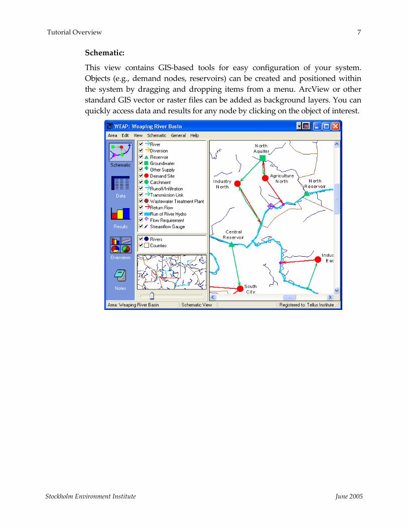
Schematic:
This view contains GIS‐based tools for easy configuration of your system. Objects (e.g., demand nodes, reservoirs) can be created and positioned within the system by dragging and dropping items from a menu. ArcView or other standard GIS vector or raster files can be added as background layers. You can quickly access data and results for any node by clicking on the object of interest.
Stockholm Environment Institute June 2005

8 WEAP Tutorial
Data:
The Data view allows you to create variables and relationships, enter assumptions and projections using mathematical expressions, and dynamically link to Excel.
Stockholm Environment Institute June 2005

Tutorial Overview 9
Results:
The Results view allows detailed and flexible display of all model outputs, in charts and tables, and on the Schematic.
Stockholm Environment Institute June 2005

10 WEAP Tutorial
Overviews:
You can highlight key indicators in your system for quick viewing.
Notes:
The Notes view provides a place to document your data and assumptions.
Stockholm Environment Institute June 2005

Tutorial Overview 11
The Tutorial Structure This complete tutorial guides you through the wide range of applications that can be covered with WEAP. The first three modules (WEAP in one hour, Basic Tools and Scenarios) present the essential elements needed for any WEAP modeling effort. The other modules present refinements that may or may not apply to your situation.
Aside from the three basic modules, the tutorial modules are designed in a way that they can be completed in any order and independently, as you see fit. They all start with the same model that you will create after completing the first three modules.
Stockholm Environment Institute June 2005
12 WEAP Tutorial
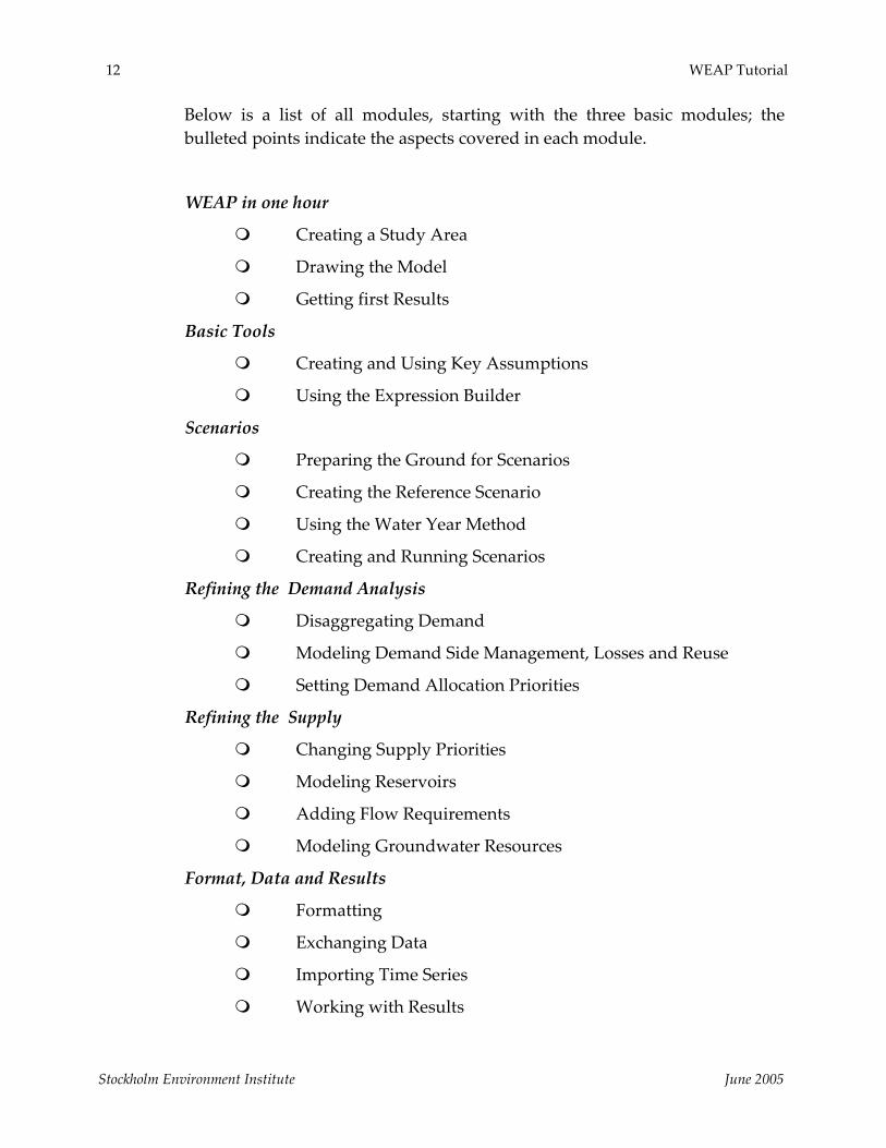
Below is a list of all modules, starting with the three basic modules; the bulleted points indicate the aspects covered in each module.
WEAP in one hour
Creating a Study Area
Drawing the Model
Getting first Results
Basic Tools
Creating and Using Key Assumptions
Using the Expression Builder
Scenarios
Preparing the Ground for Scenarios
Creating the Reference Scenario
Using the Water Year Method
Creating and Running Scenarios
Refining the Demand Analysis
Disaggregating Demand
Modeling Demand Side Management, Losses and Reuse
Setting Demand Allocation Priorities
Refining the Supply
Changing Supply Priorities
Modeling Reservoirs
Adding Flow Requirements
Modeling Groundwater Resources
Format, Data and Results
Formatting
Exchanging Data
Importing Time Series
Working with Results
Stockholm Environment Institute June 2005

Tutorial Overview 13
Reservoirs and Power Production
Modeling Reservoirs
Adding Hydropower Computation
Modeling Run‐of‐River Power Plants
Water Quality
Setting up Quality Modeling
Entering Water Quality Data
Modeling a Wastewater Treatment Plant
Hydrology
Modeling Catchments: the Rainfall Runoff Model
Modeling Catchments: the Soil Moisture Model
Simulating Surface Water‐Groundwater Interaction
Stockholm Environment Institute June 2005


WEAP Water Evaluation And Planning System
WEAP in One Hour
A TUTORIAL ON Creating a Study Area ..............................................16
Drawing the Model...................................................22
Getting first Results..................................................35
June 2005
16 WEAP Tutorial
Creating a New, Blank Study Area
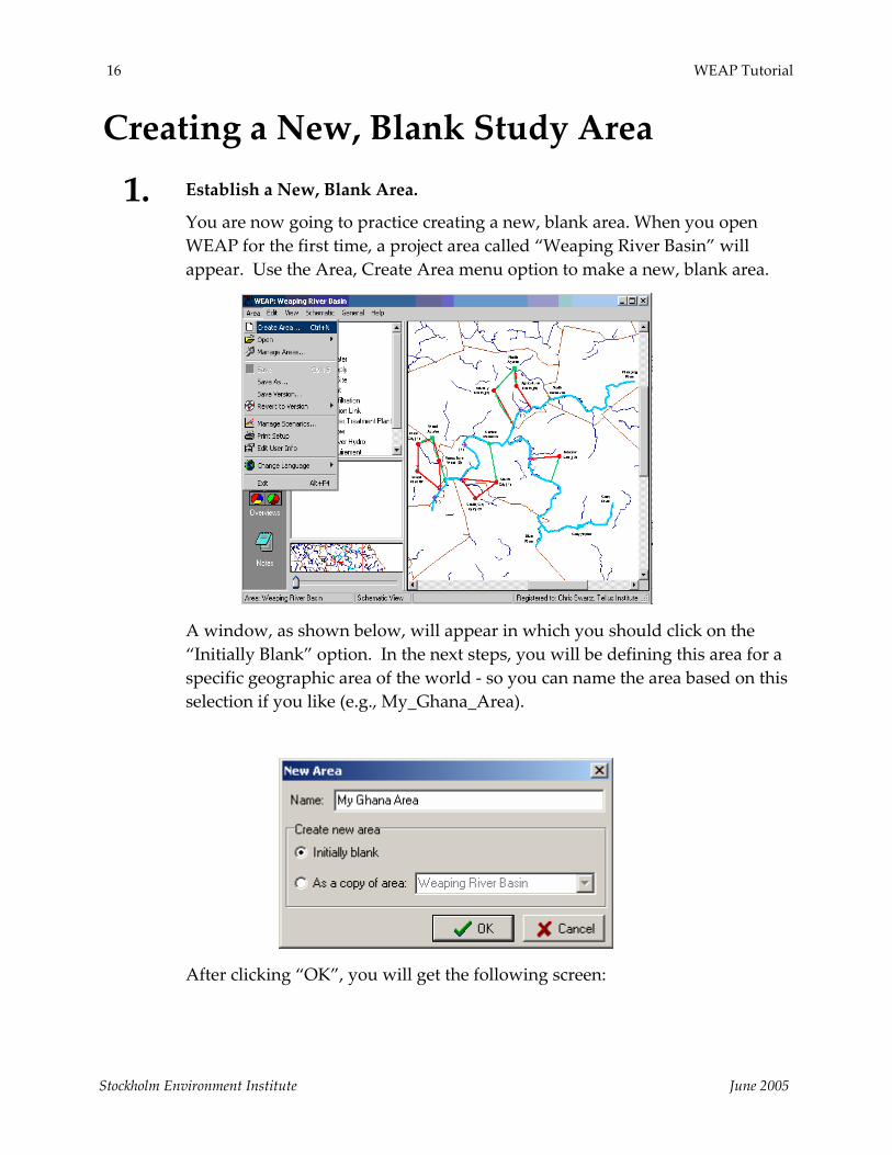
1. Establish a New, Blank Area.
You are now going to practice creating a new, blank area. When you open WEAP for the first time, a project area called “Weaping River Basin” will appear. Use the Area, Create Area menu option to make a new, blank area.
A window, as shown below, will appear in which you should click on the “Initially Blank” option. In the next steps, you will be defining this area for a specific geographic area of the world ‐ so you can name the area based on this selection if you like (e.g., My_Ghana_Area).
After clicking “OK”, you will get the following screen:
Stockholm Environment Institute June 2005
WEAP in One Hour 17
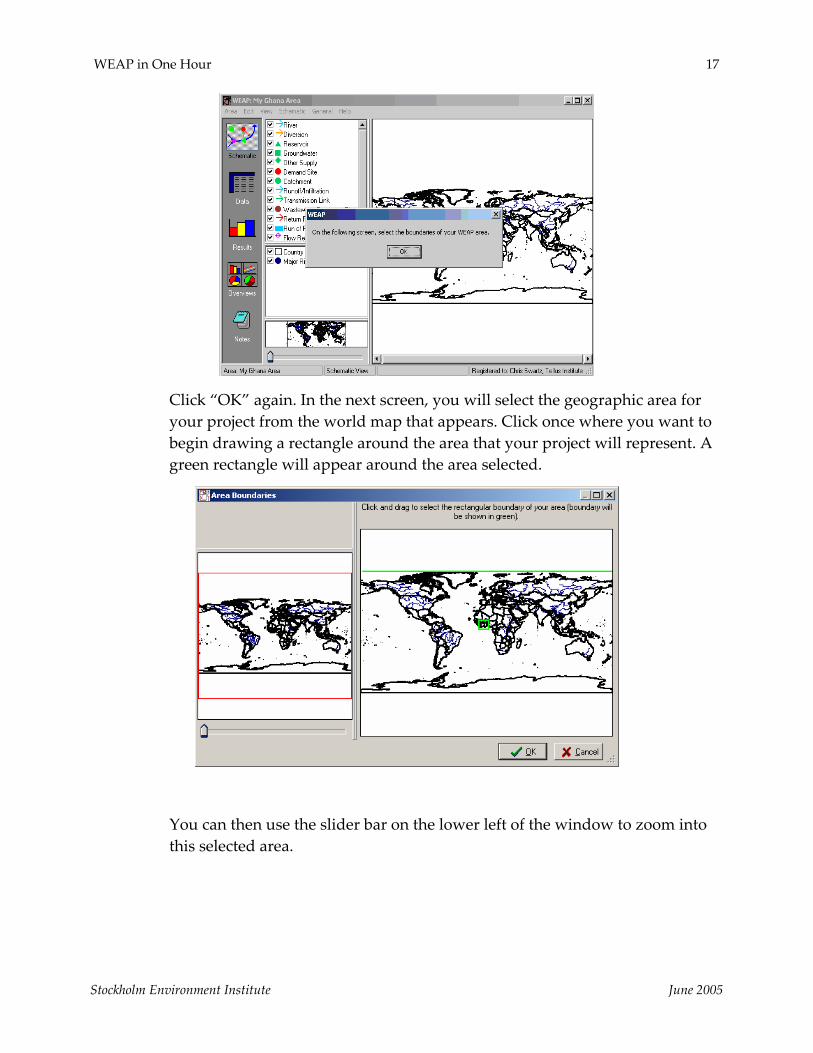
Click “OK” again. In the next screen, you will select the geographic area for your project from the world map that appears. Click once where you want to begin drawing a rectangle around the area that your project will represent. A green rectangle will appear around the area selected.
You can then use the slider bar on the lower left of the window to zoom into this selected area.
Stockholm Environment Institute June 2005

18 WEAP Tutorial
Click on “OK” when you are satisfied with your area boundaries. Note that you can modify these boundaries later by choosing “Set Area Boundaries” on the pull‐down menu under Schematic on the top menu bar.
Stockholm Environment Institute June 2005

WEAP in One Hour 19
In WEAP, models are called “areas”.
Areas are limited by boundaries, which define the extent of the project area. If you create a new area by copying an existing one, the boundary is kept identical to that of the existing area. To modify boundaries once you have established a New Area, go to Schematic on the menu, and choose “Set Area Boundaries.”
Note that if you want to start with a “blank” area, you can use the steps above to select a geographic area over one of the oceans instead of a land mass.
2. Add a GIS layer to the Area
You can add GIS‐based Raster and Vector maps to your project area ‐ these maps can help you to orient and construct your system and refine area boundaries. To add a Raster or Vector layer, right click in the middle window to the left of the Schematic and select “Add a Raster Layer” or “Add a Vector Layer”.
A window will appear in which you can input the name of this file and where WEAP can find it on your computer or on the internet.
Background vector data can be added by clicking “Add Vector Layer”. WEAP reads vector information in the SHAPEFILE format. This format can be created by most GIS software.
A large amount of georeferenced data (both in vector and raster format) is available on the Internet, sometimes for free; websites such as www.geographynetwork.com or www.terraserver.com provide good starting points for a search. Beware that some of the downloadable data might need GIS processing before being usable in WEAP,
Stockholm Environment Institute June 2005

20 WEAP Tutorial
especially to adapt the projection and/or coordinate system.
3. Saving an Area
If you want to save this Area for your own use later, Use the “Area”, “Save…” menu or press Ctrl+S.
Setting General Parameters We are now going to proceed with learning how to navigate through WEAP and its functionalities. For the remaining exercises in this tutorial we will be using a pre‐defined Area called “Tutorial”.
To open this Area, on the Main Menu, go to Area and select “Open”. You should see a list of Areas that includes “Tutorial” ‐ select this Area.
1. Set the General Parameters
Once the Area opens, use the “General” menu to set Years and Time Steps and Units.
Model the year 2000 with 12 time steps per year, based on calendar years and starting in January. Keep the default (SI units) for now. Set the period of time for which scenarios will be generated from 2000 to 2005.
Stockholm Environment Institute June 2005

WEAP in One Hour 21
The year 2000 will serve as the “Current Accounts” year for this project. The Current Accounts year is chosen to serve as the base year for the model, and all system information (e.g., demand, supply data) is input into the Current Accounts. The Current Accounts is the dataset from which scenarios are built from. Scenarios explore possible changes to the system in future years after the Current Accounts year. A default scenario, the “Reference Scenario” carries forward the Current Accounts data into the entire project period specified (here, 2000 to 2005) and serves as a point of comparison for other scenarios in which changes may be made to the system data. There will be a more detailed discussion of scenarios in an upcoming module.
Stockholm Environment Institute June 2005

22 WEAP Tutorial
The time steps must be chosen to reflect the level of precision of the data available. A shorter time step will increase the calculation time, especially when several scenarios have to be calculated.
2. Save a version of your Area
Select “Save Version” under the “Area” menu. A window will appear asking for a comment to describe this version. Type “general parameters set”.
As with any other program, it is usually a good idea to regularly save your work in WEAP. WEAP manages all the files pertaining to an area for you. Saving a new area will automatically save the related files. The files are saved in the WEAP program installation folder. You can manage the areas, export and import them, back them up and send them per email using the Area…, Manage Areas menu.
WEAP also has a very convenient versioning feature that allow saving versions of a model within the same area. Use the “Area”, “Save Version…:” menu to save a version, and the “Area”, “Revert to Version” to switch to another version. You can switch between recent and older versions without losing data. WEAP will automatically create versions of your model every time you save. It is however better to manually create a version of a status you really want to keep since WEAP will eventually delete old automatic versions to save disk space, keeping only a few.
Stockholm Environment Institute June 2005

WEAP in One Hour 23
Entering Elements into the Schematic
3. Draw a River
Click on the “River” symbol in the Element window and hold the click as you drag the symbol over to the map. Release the click when you have positioned the cursor over the upper left starting point of the main section of the river. Move the cursor, and you will notice a line being generated from that starting point.
The direction of drawing matters: the first point you draw will be the head of the river from where water will flow. You can edit the river course later on by simply clicking‐moving any part of the river to create a new point, or right‐clicking any point to delete it.
Follow the main river, drawing from the upper left to the lower right, clicking once to end each segment that you draw. You can follow the line of the river as closely as you like, or you can draw a less detailed representation (below). Zooming in on the river (using the zooming bar in the lower schematic window) can help if you want to follow the rivers path more closely. You do not need to draw a river on the branch coming horizontally from the left. You can also adjust the river later if you want to add more detail.
Stockholm Environment Institute June 2005

24 WEAP Tutorial
When you double click to finish drawing the river, a dialog box appears for naming the river (see below).
Name the river ʺMain Riverʺ.
You may also enter an optional label for the schematic presentation (a shorter label can help to keep the schematic from becoming cluttered).
Stockholm Environment Institute June 2005

WEAP in One Hour 25
You can move the river label to another location by right clicking anywhere on the river and selecting ʺMove Labelʺ. The label will follow the cursor ‐single click when the label is in the desired location.
4. Enter Data for the Main River
To enter and edit data for the Main River, either right‐click on the Main River and select Edit data and any item in the list, or switch to the Data view by clicking on the Data symbol on the left of the main screen. Select: Supply and Resources/ River /Main River in the Data tree. You may have to click on the “plus sign” icon beside the Supply and Resources branch in order to view all of the additional branches below it in the tree.
Stockholm Environment Institute June 2005

26 WEAP Tutorial
Alternatively, you can use the Tree pull‐down menu and select “Expand All” to view all branches.
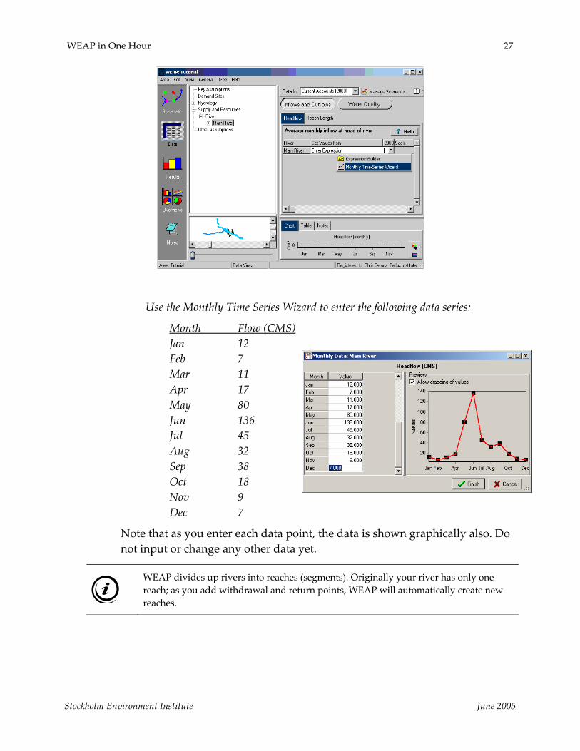
The ʺInflows and Outflowsʺ window should be open ‐ if it isnʹt, click on the appropriate button. Click on the ʺHeadflowʺ tab. Click on the area just beneath the bar labeled “2000” in the data input window to view a pull‐down menu icon. Select the “Monthly Time‐Series Wizard” from the drop‐‐down menu.
Stockholm Environment Institute June 2005
WEAP in One Hour 27
Use the Monthly Time Series Wizard to enter the following data series:
Month Flow (CMS) Jan 12 Feb 7 Mar 11 Apr 17 May 80 Jun 136 Jul 45 Aug 32 Sep 38 Oct 18 Nov 9 Dec 7
Note that as you enter each data point, the data is shown graphically also. Do not input or change any other data yet.
WEAP divides up rivers into reaches (segments). Originally your river has only one reach; as you add withdrawal and return points, WEAP will automatically create new reaches.
Stockholm Environment Institute June 2005

28 WEAP Tutorial
5. Create an Urban Demand Site and Enter the Related Data
Creating a demand node is similar to the process you used to create a river. Return to the Schematic view and pull a demand node symbol onto the schematic from the Element window, releasing the click when you have positioned the node on the left bank of the river (facing downstream) in the yellow area that marks the city’s extent.
Enter the name of this demand node as “Big City” in the dialog box, and set the demand priority to 1.
The Demand Priority represents the level of priority for allocation of constrained resources among multiple demand sites. WEAP will attempt to supply all demand sites with highest Demand Priority, then moving to lower priority sites until all of the demand is met or all of the resources are used, whichever happens first.
Stockholm Environment Institute June 2005

WEAP in One Hour 29
Right click on the Big City demand site and select ʺEdit dataʺ and ʺAnnual Activity Levelʺ. (This is the alternative way to edit data, rather than clicking on the ʺDataʺ view icon on the side bar menu and searching through the data tree.
You must first select the units before entering data. Pull down the ʺActivity Unitʺ window, select ʺPeople”, and click “OK”.
Stockholm Environment Institute June 2005

30 WEAP Tutorial
In the space under the field labeled”2000”, enter the Annual Activity Level as 800000.
Next, click on the ʺAnnual Water Use Rateʺ tab and enter 300 under than year 2000.
Stockholm Environment Institute June 2005

WEAP in One Hour 31
Finally, click on the ʺConsumptionʺ tab and enter 15. Note that the units are pre‐set to ʺpercentʺ.
Consumption represents the amount of water that is actually consumed (i.e. is not returned in the form of wastewater).
6. Create an Agriculture Demand Site
Pull another demand node symbol into the project area and position it on the other side of the Main River opposite and downstream of Big City.
Name this demand node ʺAgricultureʺ, and set the demand priority to 1.
Stockholm Environment Institute June 2005
32 WEAP Tutorial
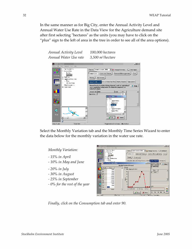
In the same manner as for Big City, enter the Annual Activity Level and Annual Water Use Rate in the Data View for the Agriculture demand site after first selecting ʺhectaresʺ as the units (you may have to click on the “plus” sign to the left of area in the tree in order to see all of the area options).
Annual Activity Level 100,000 hectares Annual Water Use rate 3,500 m3/hectare
Select the Monthly Variation tab and the Monthly Time Series Wizard to enter the data below for the monthly variation in the water use rate.
Monthly Variation:
‐ 15% in April ‐ 10% in May and June
‐ 20% in July ‐ 30% in August ‐ 25% in September ‐ 0% for the rest of the year
Finally, click on the Consumption tab and enter 90.
Stockholm Environment Institute June 2005
WEAP in One Hour 33
The monthly variation is expressed in a percentage of the yearly value. It therefore has to sum up to 100% over the full year. If you don’t specify monthly variation, WEAP will prescribe a monthly variation based on the number of days in each month.
You could have created one single demand site integrating both urban and agriculture demand. However, we will see later that this removes some of the flexibility in the water supply priorities allocation.
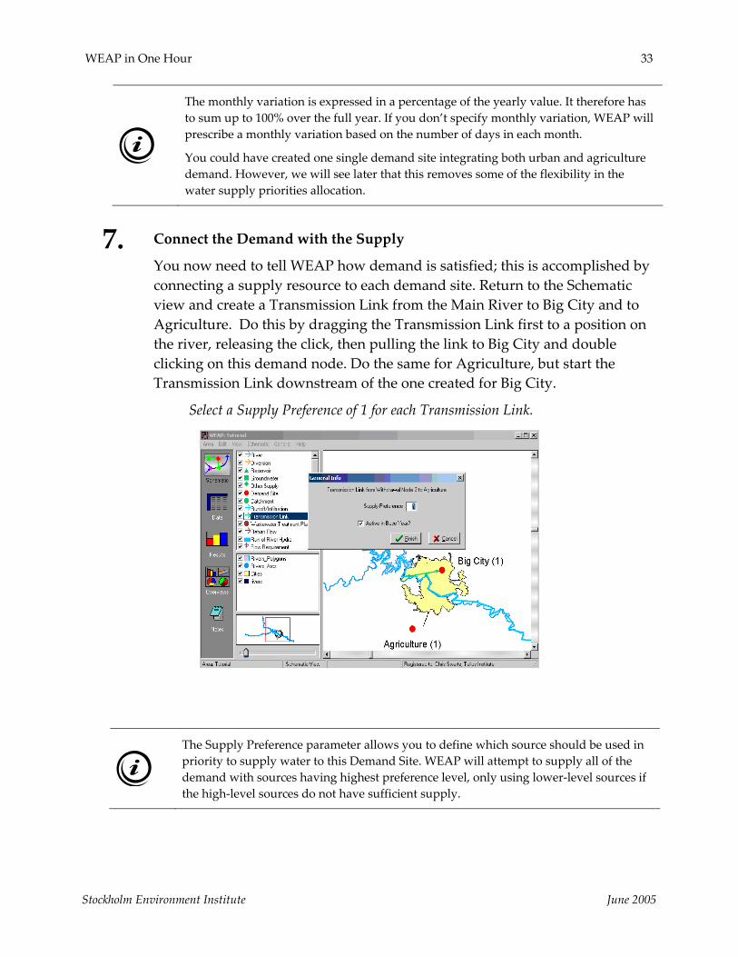
7. Connect the Demand with the Supply
You now need to tell WEAP how demand is satisfied; this is accomplished by connecting a supply resource to each demand site. Return to the Schematic view and create a Transmission Link from the Main River to Big City and to Agriculture. Do this by dragging the Transmission Link first to a position on the river, releasing the click, then pulling the link to Big City and double clicking on this demand node. Do the same for Agriculture, but start the Transmission Link downstream of the one created for Big City.
Select a Supply Preference of 1 for each Transmission Link.
The Supply Preference parameter allows you to define which source should be used in priority to supply water to this Demand Site. WEAP will attempt to supply all of the demand with sources having highest preference level, only using lower‐level sources if the high‐level sources do not have sufficient supply.
Stockholm Environment Institute June 2005

34 WEAP Tutorial
8. Create Return Flow Links
Now create a Return Flow from Big City to the Main River. Do the same for Agriculture to the Main River. Follow the same ʺdrag and releaseʺ procedure as for the Transmission Links.
The return flow for the urban demand site should be positioned downstream of the agriculture withdrawal point. In the flow direction, the sequence should be: withdrawal for City, withdrawal for Agriculture, return from City, return from Agriculture.
Next, set the Return Flow Routing for the Big City Return Flow. Do this by right‐clicking on each Return Flow and selecting ʺedit dataʺ and ʺReturn Flow Routingʺ or by going to the Data view/Supply and Resources/Return Flows/from Big City. Do the same for the Agriculture Return Flow.
Set the Return Flow Routing to 100%.
Stockholm Environment Institute June 2005

WEAP in One Hour 35
9. Check your Model
At this point, your model should look similar to the figure below.
Getting first Results
1. Run the Model
Click on the “Results” view start the computation. When asked whether to recalculate, click yes. This will compute the entire model for the Reference Scenario ‐ the default scenario that is generated using Current Accounts
Stockholm Environment Institute June 2005

36 WEAP Tutorial
information for the period of time specified for the project (here, 2000 to 2005). When the computation is complete, the Results view will appear.
2. Check your Results
Click on the Table tab and select “Demand” and “Water Demand” from the Primary Variable pull‐down menu in the upper center of the window (see below). Also, click the “Annual Total” Box.
If you have entered all data as listed in previous steps, you should obtain the following annual demand values for each year (2000 to 2005) of the Reference scenario:
Annual Demand for Agriculture 350 M m3 Annual Demand for Urban Area 240 M m3
Stockholm Environment Institute June 2005

WEAP in One Hour 37
If you do not obtain those values go back to the “Data” view and check your inputs.
If you obtain an error or warning message read it carefully as it might reveal where in your inputs is the discrepancy, or which step you skipped.
3. Look at Additional Results
Now, look at the monthly Demand Coverage rates in graphical form. Click on the “Chart” tab. Select “Demand” and “Coverage” from the Primary Variable pull‐down menu in the upper center of the window.
Stockholm Environment Institute June 2005

38 WEAP Tutorial
Format the graph by selecting the 3‐D option on the left side‐bar menu, and ensure that “All months” is selected in the pull‐down menu above the graph (also keep the “Monthly Average” option checked). The graph should like the one below (right).
During the months of December and February, which have little flow in the river, Big City lacks water, and therefore demands go unmet. Agriculture only has a shortfall in supply in the month of August and September, when the plants require most water.
You can fully customize the way WEAP charts are displayed, as well as print or copy graphs to the clipboard using the toolbox located to the right of the graph.
Stockholm Environment Institute June 2005

WEAP Water Evaluation And Planning System
Basic Tools
A TUTORIAL ON Creating and Using Key Assumptions.....................40
Using the Expression Builder ...................................43
June 2005

40 WEAP Tutorial
Note: For this module you will need to have completed the previous module (“WEAP in one hour”) or have a basic knowledge of WEAP (creating an area, drawing a model, entering basic data, obtaining first results). To begin this module, go to the Main Menu, select “Revert to Version” and choose the version named “Starting Point for ‘Basic Tools’ module.”
Creating and Using Key Assumptions
1. Using Key Assumptions
Key Assumptions are created by going to the Data view and right‐clicking on the Key Assumptions branch of the Data Tree. Select “Add” ‐ this will create a new Key Assumption variable below the Key Assumption branch.
Create and name the following Key Assumptions (be sure to select the appropriate units from the Units pull‐down menu):
Unit Domestic Water Use 300 m3 Unit Irrigation Water Needs 3,500 m3
Stockholm Environment Institute June 2005

Basic Tools 41
With Key Assumptions, it is important to ensure that the units designated in a Key Assumption variable match the units indicated for the variable as it occurs elsewhere in the data tree.
Create one more Key Assumption, Domestic Variation, that is unitless, and use the Monthly Time Series to populate it with values:
Domestic Variation ‐ Jan to Feb & Nov. to Dec.: 0.9 ‐ Mar. to May & Sept. to Oct. 1.0 ‐ June 1.1 ‐ Jul, Aug 1.15
Stockholm Environment Institute June 2005

42 WEAP Tutorial
The use of key assumptions is especially worthwhile when the model has a large number of similar objects, for example demand sites, and when performing scenario analyses. In this case, you can easily set all your demand sites to have the same unit domestic consumption. Then, you can create scenarios to vary this consumption without having to edit each and every demand site – simply by changing the key assumption value.
2. Creating References to Key Assumption
Create a Key Assumption reference for Big City Annual Water Use. Do this by going to the Annual Water Use window for Big City in the Data view. Click on the Expression Builder pull‐down menu in the space where you entered the Annual Water Use Rate (300 m3) previously.
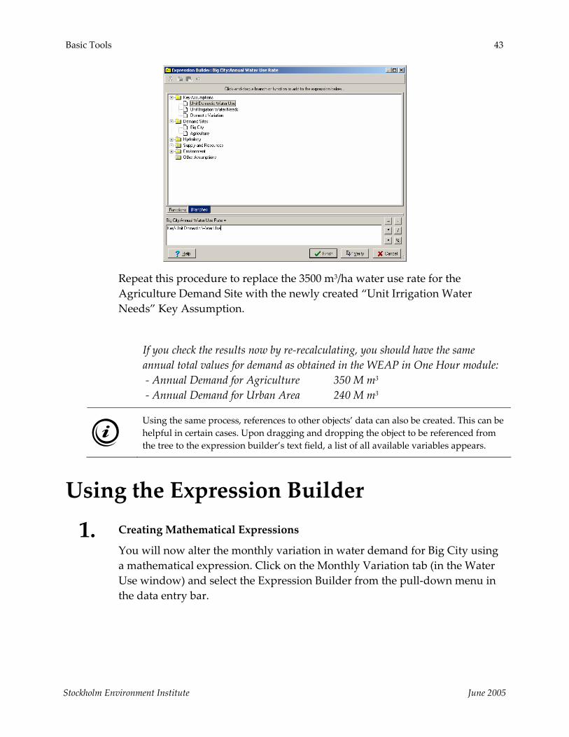
In the Expression Builder window, delete the value of 300 from the text field at the bottom of the Expression Builder window, click on the “Branches” tab, then click on the “Unit Domestic Water Rate” Key Assumption (you may have to expand the data tree to see all of the branches) in the Data tree field and drag it down to the text field. Click on “Finish”.
Stockholm Environment Institute June 2005
Basic Tools 43
Repeat this procedure to replace the 3500 m3/ha water use rate for the Agriculture Demand Site with the newly created “Unit Irrigation Water Needs” Key Assumption.
If you check the results now by re‐recalculating, you should have the same annual total values for demand as obtained in the WEAP in One Hour module: ‐ Annual Demand for Agriculture 350 M m3 ‐ Annual Demand for Urban Area 240 M m3
Using the same process, references to other objects’ data can also be created. This can be helpful in certain cases. Upon dragging and dropping the object to be referenced from the tree to the expression builder’s text field, a list of all available variables appears.
Using the Expression Builder
1. Creating Mathematical Expressions
You will now alter the monthly variation in water demand for Big City using a mathematical expression. Click on the Monthly Variation tab (in the Water Use window) and select the Expression Builder from the pull‐down menu in the data entry bar.
Stockholm Environment Institute June 2005
44 WEAP Tutorial
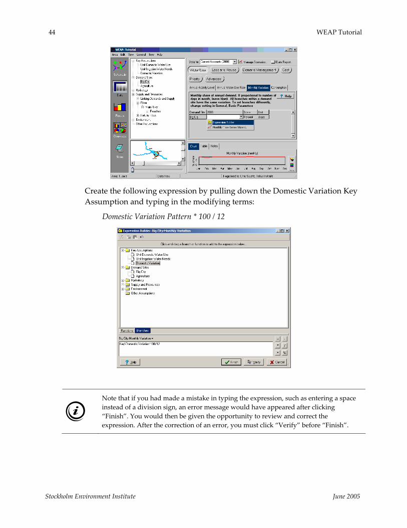
Create the following expression by pulling down the Domestic Variation Key Assumption and typing in the modifying terms:
Domestic Variation Pattern * 100 / 12
Note that if you had made a mistake in typing the expression, such as entering a space instead of a division sign, an error message would have appeared after clicking “Finish”. You would then be given the opportunity to review and correct the expression. After the correction of an error, you must click “Verify” before “Finish”.
Stockholm Environment Institute June 2005

Basic Tools 45
View the new results for Demand Site Coverage after making these changes. Click on the Results view and click on “Yes” to recalculate. The results should appear as below:
Note that there now is no unmet demand in December for the Big City because the fraction of demand in December decreased from 8.5% (originally based on the number of days in the month) to 7.5% (now based on the expression using the Domestic Variation Key Assumption). You can review the numerical values calculated from the Monthly Variation expression by selecting the “Table” tab in the data review panel at the bottom of the data window.
Stockholm Environment Institute June 2005

46 WEAP Tutorial
2. Using Built‐In Functions
We will assume that the current population of Big City (2000) is not known, but we know its population during the last census and the growth estimate. Use the built‐in “GrowthFrom” function to compute the current population of Big City. Do this by selecting the Expression Builder from the pull‐down menu in the year 2000 data input field within the Annual Activity Level window for Big City. Delete the present value of 800000, click on the “Function” tab rather than the “Branch” tab and drag down into the text field the “GrowthFrom” expression selected from the list of built in expressions.
Input the following data into the GrowthFrom expression, using the format indicated in the description window next to the expression list.
Stockholm Environment Institute June 2005

Basic Tools 47
Date of last Census 1990 Population at last census 733,530 Estimated growth rate 1.75%
This results in the following format for the expression:
GrowthFrom(1.75%, 1990, 733530)
The Expression Builder is only a simple way of entering expressions and functions. Savvy users can by‐pass it and enter functions, references and mathematical expressions directly in the main Expression window.
Stockholm Environment Institute June 2005


WEAP Water Evaluation And Planning System
Scenarios
A TUTORIAL ON Preparing the Ground for Scenarios .........................50
Creating the Reference Scenario ...............................51
Creating and Running Scenarios .............................56
Using the Water Year Method..................................59
June 2005

50 WEAP Tutorial
Note: For this module you will need to have completed the previous modules (WEAP in One Hour and Basic Tools) or have a fair knowledge of WEAP (data structure, key assumptions, expression builder). To begin this module, go to the Main Menu, select “Revert to Version” and choose the version named “Starting Point for ‘Scenariosʹ module”.
Preparing the Ground for Scenarios
1. Understand the Structure of Scenarios in WEAP
In WEAP the typical scenario modeling effort consists of three steps. First, a “Current Accounts” year is chosen to serve as the base year of the model; Current Accounts has been what you have been adding data to in the previous modules. A “Reference” scenario is established from the Current Accounts to simulate likely evolution of the system without intervention. Finally, “what‐if” scenarios can be created to alter the “Reference Scenario” and evaluate the effects of changes in policies and/or technologies.
Read the “Scenario Analysis” and “Scenarios Analysis” help topics for a more detailed description of the WEAP approach.
2. Change the Time Horizon for the Area
Under the “General”, “Years and Time Steps” menu, change the Time Horizon of the Area.
Current Accounts Year 2000 (unchanged) Last Year of Scenarios 2015
3. Create an Additional Key Assumption
Create the following key assumption:
Stockholm Environment Institute June 2005

Scenarios 51
Population Growth Rate 2.2%
There is no Unit for this Key Assumption, but remember to change the Scale field to Percent.
Creating the Reference Scenario
1. Describe the Reference Scenario
The “Reference” Scenario always exists. Change its description in the “Area”, “Manage Scenarios…” menu to reflect its actual role. Note that you must be in the Data View to have access to the “Manage Scenarios” option in the Area menu.
For example, “Base Case Scenario with population growth continuing at the 1960‐1995 rate and slight irrigation technology improvement”.
2. Change the Unit Irrigation Water Use
In the Data View, change the Unit Irrigation Water Use (an existing Key Assumption) to reflect a new annual pattern for the period (2001‐2015) after the Current Accounts year. To make the change, you will need to select the “Reference” scenario from the drop‐down menu at the top of the screen. Use the “Yearly Time‐Series Wizard” to construct the time series.
Stockholm Environment Institute June 2005

52 WEAP Tutorial
First, select the function ʺinterpolateʺ by clicking on it, then click ʺnextʺ. Click on ʺenter dataʺ in the next window, click ʺnextʺ, then click ʺaddʺ to add the following data to the time series:
Type of Time Series: Interpolate Data: 2000 3500 2005 3300 2010 3200 Growth after last year: 0%
Stockholm Environment Institute June 2005

Scenarios 53
As you can see while running the Yearly Time Series Wizard, WEAP offers a wide range of techniques to build time series, including importing from Excel files, creating step functions, using forecasting equations etc.
The Yearly Time Series Wizard does nothing else than help you create expressions. You can also simply type or edit the expression (in this case, “Interp( 2000,3300, 2005,3300, 2010,3200 )” without running the wizard, either directly, or through the Expression Builder.
Stockholm Environment Institute June 2005

54 WEAP Tutorial
3. Set the Population Growth
Set the population of Big City to grow by the rate defined by the “Population Growth Rate” key assumption defined in an earlier step. Here again you will have to select the “Reference” scenario in the drop‐down menu at the top of the Data view.
Make sure you have the Big City Demand Site and its Annual Activity Level tab selected. Delete the current expression and select the “Growth” function in the Expression Builder in the pull‐down menu below the 2001‐2015 field (Note that the present expression in this field is the same as that for the Current Accounts year). Then click on the Branch tab above the text field. Double click on the ʺPopulation Growth Rateʺ Key Assumption in the Data Tree. Your final function should read “Growth(Key\Population Growth Rate/100)”
Note that you have to divide the Population Growth Rate by 100 in order for WEAP to recognize the value of 2.2 in the Key Assumption as 0.022 in the calculation.
The same effect could have been modeled without creating a key assumption in the first place. We will see however that doing so provides more flexibility when adding other scenarios.
Any value for which no time series is defined for the “Reference” scenario is assumed to remain constant. In our case for example, the agriculture scenario will remain constant until 2015 unless we change this variable as well.
Stockholm Environment Institute June 2005
Scenarios 55
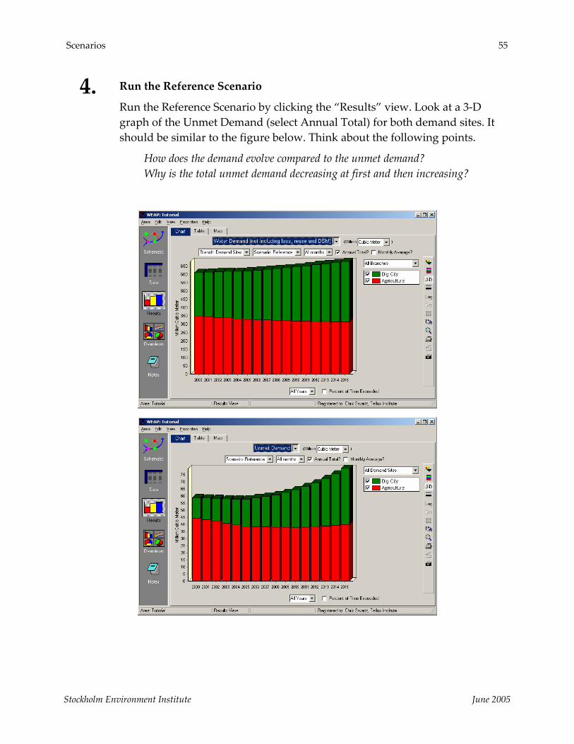
4. Run the Reference Scenario
Run the Reference Scenario by clicking the “Results” view. Look at a 3‐D graph of the Unmet Demand (select Annual Total) for both demand sites. It should be similar to the figure below. Think about the following points.
How does the demand evolve compared to the unmet demand? Why is the total unmet demand decreasing at first and then increasing?
Stockholm Environment Institute June 2005

56 WEAP Tutorial
Creating and Running Scenarios
1. Create a New Scenario to Model High Population Growth
Create a new scenario to evaluate the impact of a population growth rate for Big City higher than 2.2% for the period 2001‐2015.
For this, choose the menu “Area”, “Manage Scenario”, right‐click the “Reference” scenario and select “Add”. Name this scenario “High Population Growth” and add the description “this scenario looks at the impact of increasing the population growth rate for Big City from a value of 2.2% to 5.0%.”
Stockholm Environment Institute June 2005

Scenarios 57
2. Enter the Data for this Scenario
Make the following changes in the Data view after having chosen your new scenario in the drop‐down menu at the top of the screen:
Select the Population Growth Rate Key Assumption and change the value under the 2001‐2015 field to 5.0. Note that the color of the data field changes to red after the change ‐ this occurs for any values that are changed to deviate from the Reference scenario value.
3. Compare Results for the Reference and Higher Population Growth Scenarios
Compare, graphically, the results for the two scenarios we have established so far (Reference and Higher Population Growth).
For example, select Water Demand from the Primary Variable pull‐down menu. Click in the drop‐down menu to the right of the chart area (above the graph legend), and select “All Scenarios”. Choose to show only Big City demand by selecting it from the pull‐down list in the upper left pull‐down menu of the Results window. Your graph should be similar to the one below.
Stockholm Environment Institute June 2005

58 WEAP Tutorial
Note the higher Big City Water Demand for the Higher Population Growth scenario, as expected.
Next, compare Unmet Demand for the two scenarios. Use the Primary Variable pull‐down menu to select Unmet Demand.
Again, note the higher Unmet Demand for the Higher Population Growth scenario.
When creating many scenarios in the same area, the computation can become lengthy. In this case you can exclude some of the scenarios from the calculation by unchecking the “Show results for this scenario” box in the scenario manager for those scenarios.
Stockholm Environment Institute June 2005
Scenarios 59
Using the Water Year Method
1. Create the Water Year Definitions
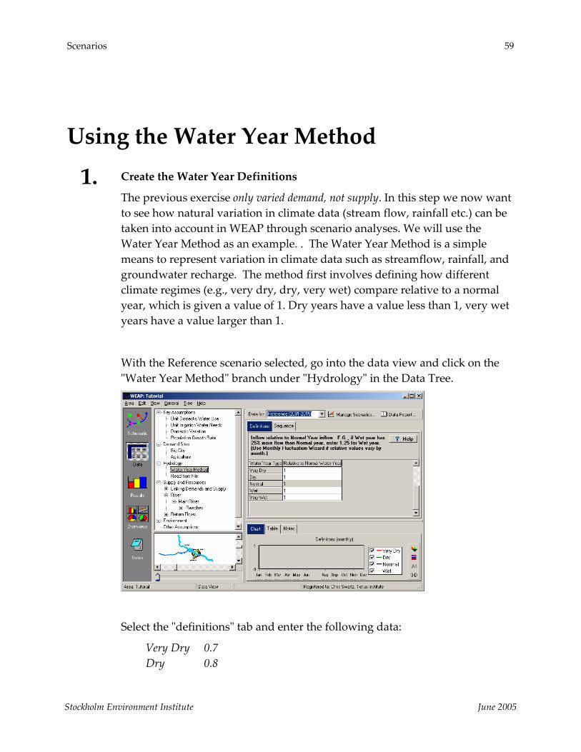
The previous exercise only varied demand, not supply. In this step we now want to see how natural variation in climate data (stream flow, rainfall etc.) can be taken into account in WEAP through scenario analyses. We will use the Water Year Method as an example. . The Water Year Method is a simple means to represent variation in climate data such as streamflow, rainfall, and groundwater recharge. The method first involves defining how different climate regimes (e.g., very dry, dry, very wet) compare relative to a normal year, which is given a value of 1. Dry years have a value less than 1, very wet years have a value larger than 1.
With the Reference scenario selected, go into the data view and click on the ʺWater Year Methodʺ branch under ʺHydrologyʺ in the Data Tree.
Select the ʺdefinitionsʺ tab and enter the following data:
Very Dry 0.7 Dry 0.8
Stockholm Environment Institute June 2005

60 WEAP Tutorial
Normal 1.0 Wet 1.3 Very wet 1.45
Monthly variations can be entered if data is available.
2. Create the Water Year Sequence
The next step in using the Water Year Method is to create the sequence of climatic variation for the scenario period. Each year of the period is assigned one of the climate categories (e.g., wet). For the Reference Scenario, we will assume the following sequence:
2001‐2003 normal 2004 very dry 2005 wet 2006‐2008 normal 2009‐2010 dry 2011 very wet
Stockholm Environment Institute June 2005

Scenarios 61
2012 normal 2013 wet 2014 normal 2015 dry
To input this sequence, select the ʺSequenceʺ tab under the ʺWater Year Methodʺ branch.
Set the Current Account as Normal
Then, select the Reference scenario and input the sequence given above.
In order to let the inflows to the model (in our case, the headflow of the main river) vary in time, WEAP offers two strategies. If detailed forecasts are available, those can be read using the ReadFromFile function (refer to the Tutorial module on Format and Data for
Stockholm Environment Institute June 2005

62 WEAP Tutorial
more details). Another method, which is the one presented here, is the “Water Year Method”. Under this method every year in the model’s duration can be defined as normal, wet, very wet, dry or very dry. Different scenarios can then alter the chosen sequence of dry and wet years to assess the impact of natural variation on water resources management.
3. Set up the Model to Use the Water Year Method
In the Data Tree, change the Headflow for the Main River in the “Reference” scenario to use the “Water Year Method”. Note that before, the monthly values of headflow were the same for the period 2001‐2015 as for 2000, the Current Accounts year.
Use the drop down menu in the “Get Values from” to select this method. You may have to scroll left in this window to get the “Get Values from” field to appear
4. Re‐run the Model
Run the model again and compare Unmet Demand for the Reference and Higher Population Growth scenarios, as before (of course, Water Demand will not have changed after altering the supply side of the model with the Water Year Method).
Stockholm Environment Institute June 2005

Scenarios 63
Note that Big City Unmet Demand for both scenarios is much more erratic using the Water Year Method than assuming a constant headflow to the Main River, as observed in the previous exercise. In the present case, the Unmet Demand varies as the future climate varies. During years wetter or much wetter than normal (2000, the Current Accounts year), Unmet Demand is actually lower than in 2000 for both scenarios, even with the increase in Water Demand from population growth (2.2% for the Reference and 5.0% for the Higher Population Growth scenarios). The increased precipitation, and headflow to the river, mitigates this increased demand in the wetter years.
The opposite occurs in the dry to very dry years, where the population growth is exacerbated by the lower precipitation and headflow in the river in these years. This leads to even higher Unmet Demand than is simulated assuming a constant climate (as performed in the previous exercise).
Since unmet demand is the difference between a large demand and a large supply, even a rather small change in the supply at nearly‐constant demand can have a very large impact on the unmet demand.
This model does not take any kind of inter‐year storage into consideration (reservoirs, groundwater). Therefore, there is no way that the shortage in a dry year can be alleviated by using surplus from previous, wetter years. For more details on how to model storage, refer to the “Supply” WEAP tutorial module.
If you had wanted to compare, in the same graph in WEAP, results for the Water Year Method to that generated assuming a constant climate, you could
Stockholm Environment Institute June 2005

64 WEAP Tutorial
have created a new scenario that used the Water Year Method rather than changing the data in the Reference Scenario to accommodate the Water Year Method. This new scenario would be inherited from the Reference scenario, and the scenario tree in the Scenarios Manager would look as follows:
Note that in this case, both the Reference (constant climate) and Water Year Scenarios (variable climate) would use a Population Growth Rate equal to 2.2% for Big City, since the Water Year Scenario is inherited from the Reference Scenario. If one wanted to compare, in the same WEAP graph, constant climate and variable climate using a 5% Population Growth Rate, you could create another new scenario inherited from the Water Year scenario and change the Population Growth Rate Key Assumption in this scenario to 5% ‐ the tree structure would look as follows:
Stockholm Environment Institute June 2005

Scenarios 65
WEAP allows for unlimited versatility in the arrangement of scenarios. Note that you can output results to Excel, which also facilitates results comparisons among scenarios. This feature will be discussed in greater detail in the Data, Results, and Formatting module.
5. Change Scenario Inheritance
The following example demonstrates the utility of changing scenario inheritance within WEAP.
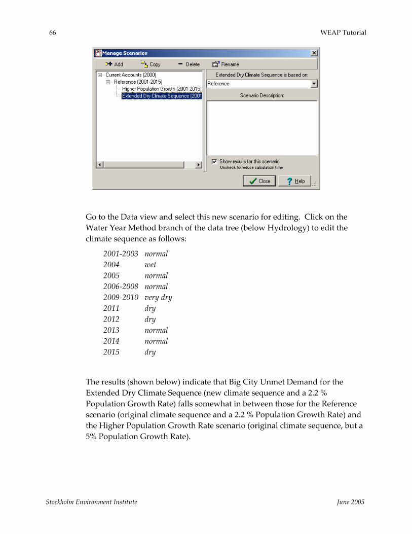
Create a new scenario inherited from the Reference scenario, and name it “Extended Dry Climate Sequence”. The scenario tree structure should look as follows:
Stockholm Environment Institute June 2005
66 WEAP Tutorial
Go to the Data view and select this new scenario for editing. Click on the Water Year Method branch of the data tree (below Hydrology) to edit the climate sequence as follows:
2001‐2003 normal 2004 wet 2005 normal 2006‐2008 normal 2009‐2010 very dry 2011 dry 2012 dry 2013 normal 2014 normal 2015 dry
The results (shown below) indicate that Big City Unmet Demand for the Extended Dry Climate Sequence (new climate sequence and a 2.2 % Population Growth Rate) falls somewhat in between those for the Reference scenario (original climate sequence and a 2.2 % Population Growth Rate) and the Higher Population Growth Rate scenario (original climate sequence, but a 5% Population Growth Rate).
Stockholm Environment Institute June 2005

Scenarios 67
Now, we will change the Scenario Inheritance of the Extended Dry Climate Sequence, placing it under the Higher Population Growth Rate scenario so that it inherits the 5% Population Growth Rate of that scenario. In the Scenario Manager, select the Extended Dry Climate Sequence scenario, click on the drop down list to the right (below the text saying “Extended Dry Climate Sequence is based on:”) and select “Higher Population Growth” as the new parent scenario.
Now, recalculate the results and look again at Unmet Demand for Big City.
Stockholm Environment Institute June 2005

68 WEAP Tutorial
What changes do you notice to the unmet demand for the Extended Dry Climate Sequence?
With the higher population growth rate and dryer climate, Unmet Demand increases substantially.
Stockholm Environment Institute June 2005

WEAP Water Evaluation And Planning System
Refining the Demand Analysis
A TUTORIAL ON Disaggregating Demand...........................................70
Modeling Demand Side Management, Losses and Reuse.......................................................77
Setting Demand Allocation Priorities ......................86
June 2005

70 WEAP Tutorial
Note: For this module you will need to have completed the previous modules (“WEAP in One Hour, Basic Tools, and Scenarios) or have a fair knowledge of WEAP (data structure, key assumptions, expression builder, creating scenarios). To begin this module, go to the Main Menu, select “Revert to Version” and choose the version named “Starting Point for all modules after ‘Scenarios’ module.”
Disaggregating Demand
1. Create a new Demand Site
In the Current Accounts, create a new demand site downstream of Big City to simulate rural demand. Name this node “Rural” and give it a Demand Priority = 1. Provide a Transmission Link from the Main River positioned downstream of the Big City Return Flow, but upstream of the Agriculture Return Flow. The Supply Preference should be set to 1. Also provide a Return Flow for Rural positioned upstream of Agriculture Return Flow.
Your area should now look as follows:
2. Create the Data Structure for “Rural” demand node
In order to create a data structure, right‐click the “Rural” demand site in the data view tree, and select “Add” to implement the following structure (do not enter any data yet):
Stockholm Environment Institute June 2005

Refining the Demand Analysis 71
Note that “Showers”, “Toilets”, “Washing”, and “Others” are added as sub‐branches below “Single Family Houses”.
3. Enter the Annual Activity Level data
Enter the following data under the Rural Demand Site, Annual Activity Level tab:
Rural 120,000 Households Single Family Houses 70% Share Showers 80% Saturation Toilets 90% Saturation Washing 55% Saturation Others 35% Saturation Apartment Buildings Remainder share (use the Expression Builder)
Stockholm Environment Institute June 2005

72 WEAP Tutorial
Stockholm Environment Institute June 2005
Refining the Demand Analysis 73
Share vs. Saturation: even though both types of percentages are treated mathematically the same by WEAP, they are conceptually different. At a given level of the tree, shares should always sum up to 100%. They also allow the use of the “remainder” function. Saturation indicates the penetration rate for a particular device and is independent of the penetration rate for other devices (i.e., saturation rates for all sub‐branches within a given branch do not have to sum to 100.
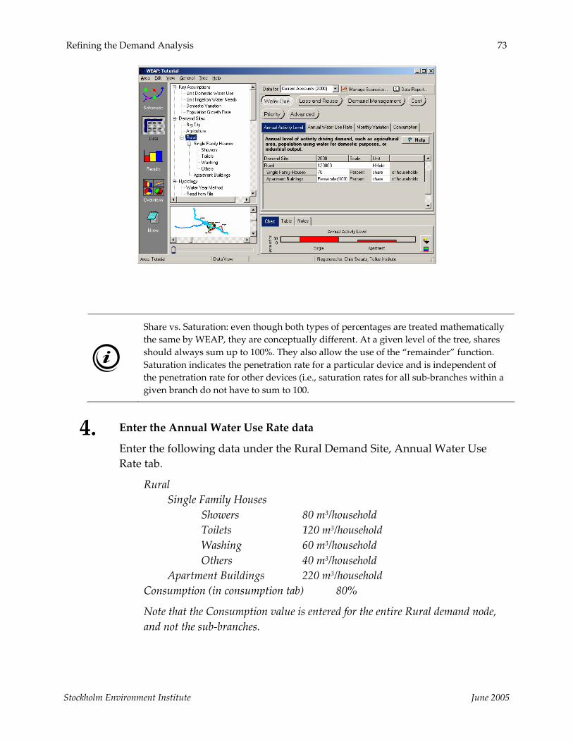
4. Enter the Annual Water Use Rate data
Enter the following data under the Rural Demand Site, Annual Water Use Rate tab.
Rural Single Family Houses Showers 80 m3/household Toilets 120 m3/household Washing 60 m3/household Others 40 m3/household Apartment Buildings 220 m3/household Consumption (in consumption tab) 80%
Note that the Consumption value is entered for the entire Rural demand node, and not the sub‐branches.
Stockholm Environment Institute June 2005

74 WEAP Tutorial
5. Check the results
Recalculate your results. You should get an error message, as pictured below. Note that a Return Flow percentage was not input when the Return Flow link for the Rural demand node was created.
Return to the data view and input a value of 100% for the Return Flow Routing for the Rural demand node.
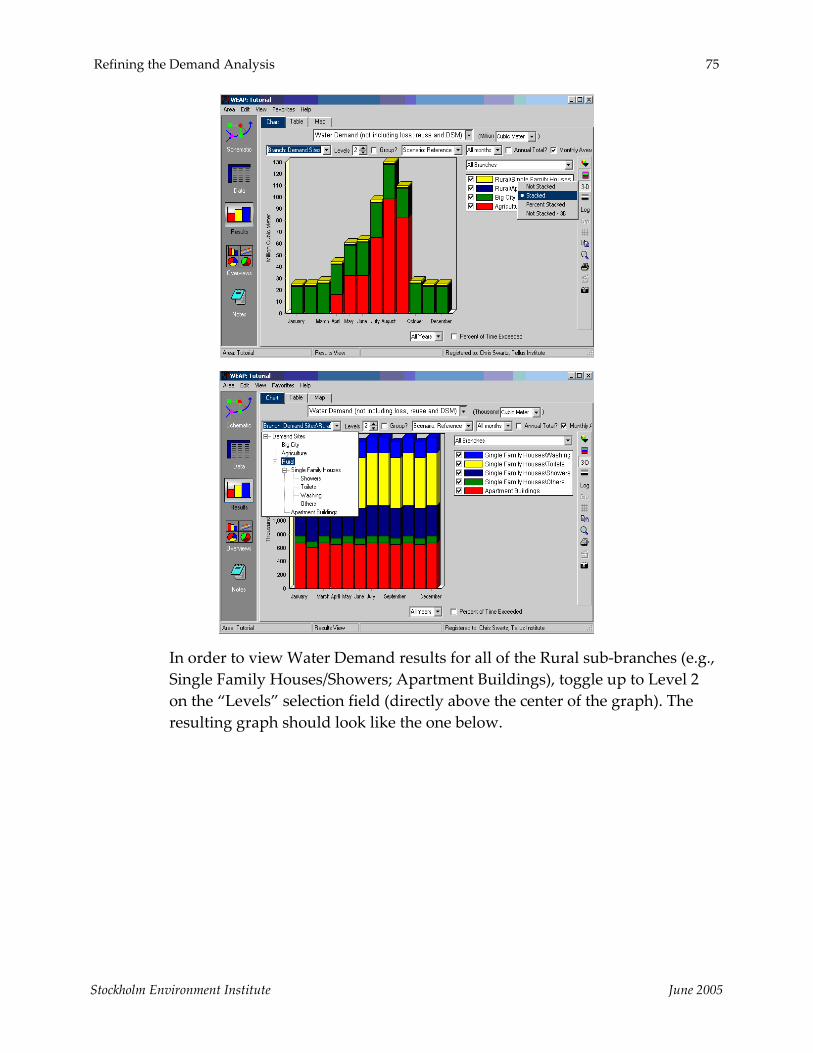
Now recalculate again. In the Results view, choose Water Demand as the Primary Variable from the pull down menu. Select “All Branches” from the pull‐down menu directly above the graph legend. Select 3‐D and bar graph as the format using the pull‐down menu for the “Chart Type” icon on the vertical graphing toolbar (see first and second screen shot below). Select the Rural demand node from the pull down menu above the graph (see third screen shot below).
Stockholm Environment Institute June 2005
Refining the Demand Analysis 75
In order to view Water Demand results for all of the Rural sub‐branches (e.g., Single Family Houses/Showers; Apartment Buildings), toggle up to Level 2 on the “Levels” selection field (directly above the center of the graph). The resulting graph should look like the one below.
Stockholm Environment Institute June 2005

76 WEAP Tutorial
Do you understand why the rural demand varies along the year even though we have not entered any variation?
The variation in Rural demand is due to the fact that WEAP assumes a constant daily demand per day (no monthly demand was specified by the user), so months that have less days (like February) have a lower demand than months that have more days (like January).
Now create a 3‐D graph of Demand Site Coverage and select all demand sites for presentation (the pull‐down menu to do the latter is to the right of the graph; see below).
Stockholm Environment Institute June 2005
Refining the Demand Analysis 77
Do you understand why the coverage is always 100% for rural but not for Big City and Agriculture, even though they all have the same demand priority level?
The Rural withdrawal point is downstream of the return flow point for the Big City, which means there is an additional volume of water available in the river; this return flow can easily cover the rather small Rural demand.
Modeling Demand Side Management, Losses and Reuse
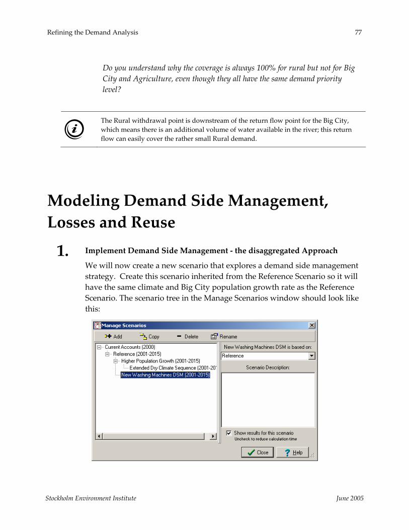
1. Implement Demand Side Management ‐ the disaggregated Approach
We will now create a new scenario that explores a demand side management strategy. Create this scenario inherited from the Reference Scenario so it will have the same climate and Big City population growth rate as the Reference Scenario. The scenario tree in the Manage Scenarios window should look like this:
Stockholm Environment Institute June 2005

78 WEAP Tutorial
We will assume that a new type of washing machines allows a 2/3 reduction (66.7%) in washing water consumption. This new scenario will evaluate the impact of this Demand Side Management measure if 50% of the households can be convinced to purchase the water‐saving machine.
First, go back to Current Accounts in the Data view, where you will create two new branches (Old Machines and New Machines) in the Rural data structure. Effectively, you are disaggregating the Washing variable to now include two new sub‐categories. Note that you must return to Current Accounts because all new data structures have to be entered in Current Accounts, even if the variable is not to be activated (i.e., given non‐zero activity levels) in the Current Accounts and Reference Scenario.
When you go to add the first sub‐branch under Washing, you will get the following message:
Click yes, and add the following structure:
Stockholm Environment Institute June 2005

Refining the Demand Analysis 79
Change the units for Old Machines and New Machines to Shares. Reenter the Water Use Rate for Old Machines (60 m3/household), as was the value for the original higher level variable “Washing”.
Enter a value of 100% for the Old Machines Activity Level. Leave blank the Activity Level for New Machines ‐ this is the same as entering a zero. Remember, you are entering these in the Current Accounts, so you want only the Old Machines to be active in the Reference scenario. This recreates the same effect as having the aggregated variable “Washing” in the original Current Accounts and Reference scenario. The New Machines variable will be activated in the New Washing Machines DSM scenario (see below).
Stockholm Environment Institute June 2005

80 WEAP Tutorial
Now, switch to the New Washing Machines DSM scenario.
Input a value of 50 for New Machines (50% of all washing machines will be this new variety) and Remainder(100) for Old Machines (use the Expression Builder for the latter).
You will have to input again the original Water Use Rate for the Old Machines (60 m3/household) as well as the new Water Use Rate for the New Machines:
Old Machines 60 m3/household
New Machines 60*0.667 m3/household
Stockholm Environment Institute June 2005

Refining the Demand Analysis 81
Now compare the numerical Water Demand results for the Washing branch of the Rural demand site for the Reference and New Washing Machines DSM scenarios. In the Results view, click on the Table tab and select the Water Demand variable. Also select Annual Total rather than Monthly Average and choose 2001 (you can only view numerical results for one individual year at a time when comparing scenarios in the Table view, but this does not present a difficulty for this example, as we do not try to model any growth with time for the Washing variable). Choose the Demand Sites\Rural\Washing\Single Family Houses\Washing from the upper left pull‐down menu and All Branches from the upper left pull‐down menu. Select the Reference and New Washing Machines DSM scenarios from the pull‐down menu at the bottom of the window. The table should look like the following:
Stockholm Environment Institute June 2005

82 WEAP Tutorial
Note that the use of the New Machines in 2001 (and all subsequent years in the New Washing Machines DSM scenario period) results in about 460000 m3 less water demand than if only Old Machines are used (Reference scenario).
Demand‐side management (DSM) refers to measures that can be taken on the consumer’s side of the meter to change the amount or timing of water consumption (as compared to the utility companyʹs, or supply, side of the meter).
Another way of modeling disaggregated DSM is to reduce the unit consumption for the affected category (in this case washing). There is no right or wrong way to model DSM.
2. Implement Demand Side Management ‐ the aggregated Approach
If disaggregated data is not available, an equivalent value of DSM can be computed. In this example, assuming we had not disaggregated the Rural water demand, we could come to the same result by using the “Demand Management” option for this Demand Site in the Data view tab. In this case the reduction would amount to:
Original contribution of washing to rural water use 2,772/26,316 = 10.5% Share of New Machines 50% Reduction of New Machines 66.6%
Stockholm Environment Institute June 2005

Refining the Demand Analysis 83
Multiplying all of these percentages together = 3.5%
This value can be entered in the Demand Management/Demand Savings tab for the Rural branch of a Demand Side Management scenario.
Demand Side Management (DSM) measures are not taken into account in the demand view. To see the effect of a DSM measure, look at the change in Supply Requirement rather than Water Demand.
3. Model Reuse
Another water conservation strategy that could be studied with scenarios is water reuse. Create a new scenario inherited from the Reference scenario and name it “Big City Reuse”. Make sure you are in this new scenario and click on the Big City branch. Click on the Loss and Reuse button and click the Reuse tab. Enter the following expression in the 2001‐2015 field using the Expression Builder:
Smooth(2000,15, 2005,22, 2015,25)
First, pull the Smooth function into the text field of the Expression builder and select “smooth” from the options. Click “Next” and enter the data values. You should get a plot like the one below. Click “Finish”.
Stockholm Environment Institute June 2005

84 WEAP Tutorial
Compare Unmet Demand for Big City before (Reference) and after (Big City Reuse) instituting this conservation strategy. You should get the graph below, which shows substantial reductions in Big City Unmet Demand when the water reuse strategy is used.
4. Model Losses
Re‐edit the model to take into account the fact that there is a 20% loss rate in the network of Big City. Make this change for the Current Accounts so that it
Stockholm Environment Institute June 2005
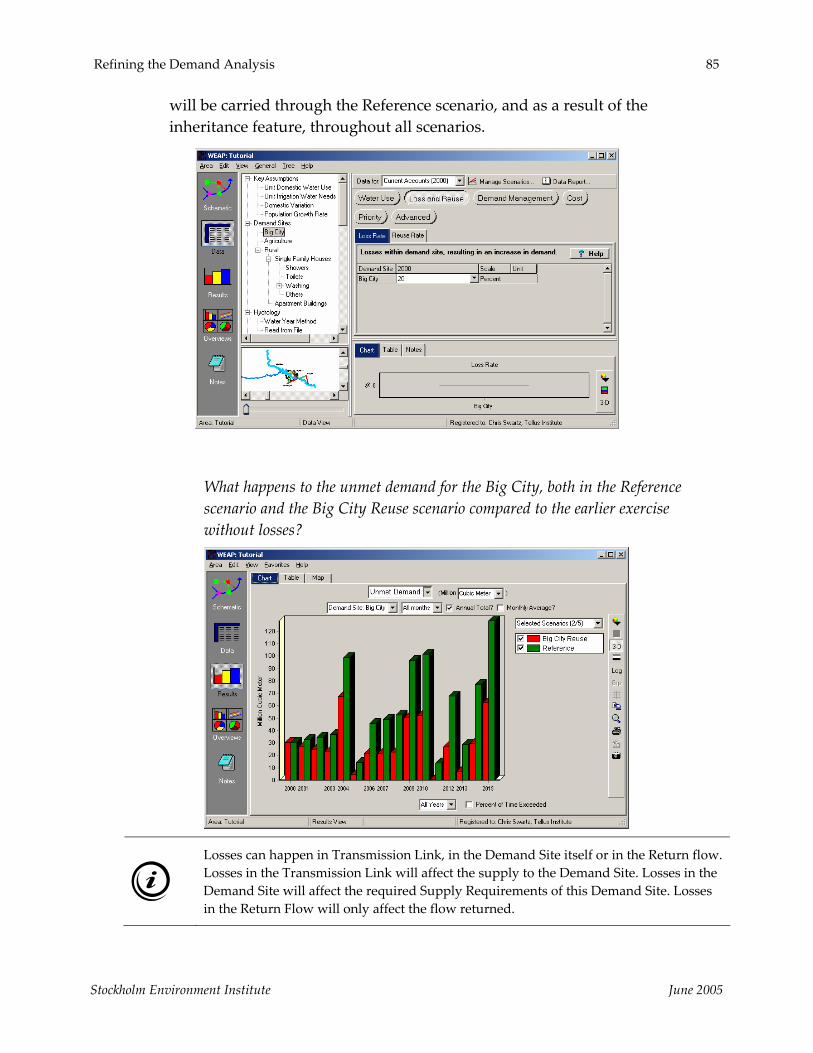
Refining the Demand Analysis 85
will be carried through the Reference scenario, and as a result of the inheritance feature, throughout all scenarios.
What happens to the unmet demand for the Big City, both in the Reference scenario and the Big City Reuse scenario compared to the earlier exercise without losses?
Losses can happen in Transmission Link, in the Demand Site itself or in the Return flow. Losses in the Transmission Link will affect the supply to the Demand Site. Losses in the Demand Site will affect the required Supply Requirements of this Demand Site. Losses in the Return Flow will only affect the flow returned.
Stockholm Environment Institute June 2005

86 WEAP Tutorial
Setting Demand Allocation Priorities
1. Edit Demand Site Priority
Create a new scenario, inherited from the Reference, and name it “Changing Demand Priorities”. Change the Demand Priority of the Agriculture Demand Site in the Data view by clicking on the Agriculture branch and then clicking on the Priority button. and on the node in the Schematic View and selecting ʺGeneral Infoʺ.
Change the Demand Priority from 1 to 2.
A demand priority can be any whole number between 1 and 99 (99 is the default) and allows the user to specify the order in which the water requirements of demand sites are satisfied. WEAP will attempt to satisfy the water requirement of a demand site with a demand priority of 1 before a demand site with a demand priority of 2 or greater. If two demand sites have the same priority, WEAP will attempt to satisfy their water requirements equally. Absolute values have no significance for the priority levels; only the relative order matters. For example, if there are two demand sites, the same result will occur if demand priorities are set to 1 and 2 or 1 and 99.
Demand Priorities allow the user to represent in WEAP water allocation as it actually occurs in their system. For example, a downstream farmer may have historical water rights to river water, even though another demand site positioned upstream could extract as much river water as it desired, leaving the farmer with little water in the absence of such water rights. The Demand Priority setting allows the user to set the farmerʹs priority for water above that of the upstream demand site. Demand Priorities can also change with time or change in a scenario ‐ more advanced subject matter to be
Stockholm Environment Institute June 2005
Refining the Demand Analysis 87
dealt with later in the tutorial.
You can also change the Demand Priority in the Data View, Priority screen, Demand Priority tab.
2. Compare Results
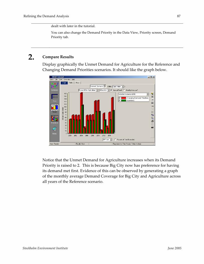
Display graphically the Unmet Demand for Agriculture for the Reference and Changing Demand Priorities scenarios. It should like the graph below.
Notice that the Unmet Demand for Agriculture increases when its Demand Priority is raised to 2. This is because Big City now has preference for having its demand met first. Evidence of this can be observed by generating a graph of the monthly average Demand Coverage for Big City and Agriculture across all years of the Reference scenario.
Stockholm Environment Institute June 2005

88 WEAP Tutorial
Now compare these results to the same graph generated for the Changing Demand Priorities scenario.
Notice that in the Reference scenario, for the spring and late summer months, both Big City and Agriculture do not get full coverage of their demand because they both compete equally for Main River flow. When Big City is given preference for meeting demand (Changing Demand Priorities scenario), however, its coverage improves relative to Agriculture. When coverage is 100% for Agriculture, but not for Big City, that is because there is no
Stockholm Environment Institute June 2005

Refining the Demand Analysis 89
Agriculture demand (primarily observed for the winter months). Note that the Demand Coverage for the Rural demand site is always 100% ‐ this is because the return flows for Big City and Agriculture satisfy the water demand created by the Rural demand site.
Stockholm Environment Institute June 2005


WEAP Water Evaluation And Planning System
Refining the Supply
A TUTORIAL ON Changing Supply Priorities ......................................92
Modeling Reservoirs .................................................95
Adding Flow Requirements ....................................101
Modeling Groundwater Resources .........................104
June 2005

92 WEAP Tutorial
Note: For this module you will need to have completed the previous modules (“WEAP in One Hour, Basic Tools, and Scenarios) or have a fair knowledge of WEAP (data structure, key assumptions, expression builder, creating scenarios). To begin this module, go to the Main Menu, select “Revert to Version” and choose the version named “Starting Point for all modules after ‘Scenarios’ module.”
Changing Supply Priorities
1. Create a new Transmission Link for water reuse
Create a new transmission link starting at the Big City Demand Site and ending at the Agriculture Demand Site. This is a conceptual model of reuse of urban wastewater for agriculture purposes. Set the Supply Preference on this Transmission Link to 2.
Supply Preference 2
If water quality were a concern, a wastewater treatment plant could have been added to treat the water from Big City before Agriculture received it. Having the treatment plant in the schematic would make it possible to simulate the changes in water quality before and after treatment.
Stockholm Environment Institute June 2005
Refining the Supply 93
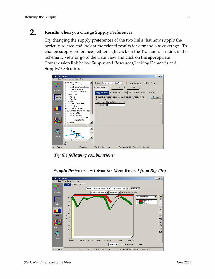
2. Results when you change Supply Preferences
Try changing the supply preferences of the two links that now supply the agriculture area and look at the related results for demand site coverage. To change supply preferences, either right click on the Transmission Link in the Schematic view or go to the Data view and click on the appropriate Transmission link below Supply and Resources/Linking Demands and Supply/Agriculture.
Try the following combinations:
Supply Preferences = 1 from the Main River, 2 from Big City
Stockholm Environment Institute June 2005

94 WEAP Tutorial
Supply Preferences = 2 from the Main River, 1 from Big City
Supply Preferences = 1 from the Main River and 1 from Big City
Do you understand why the differences in Demand Coverage occur when the Supply Preferences change?
Stockholm Environment Institute June 2005
Refining the Supply 95
You can modify the display of preferences on the schematic by using the Schematic, Change the Priority View menu. The “View Allocation Order” option will display the actual priority order in which WEAP computes supply. This is a function of the Supply Preference of the link as well as the Demand Priority of the demand site.
Note that you can study the impact of changing Supply Preferences, like Demand Priorities, by creating alternative scenarios.
3. Revert to original model
You can do this by deleting the transmission link between Big City and Agriculture and making sure the Supply Preference for the link between the Main River and Agriculture area is set to 1.
Modeling Reservoirs
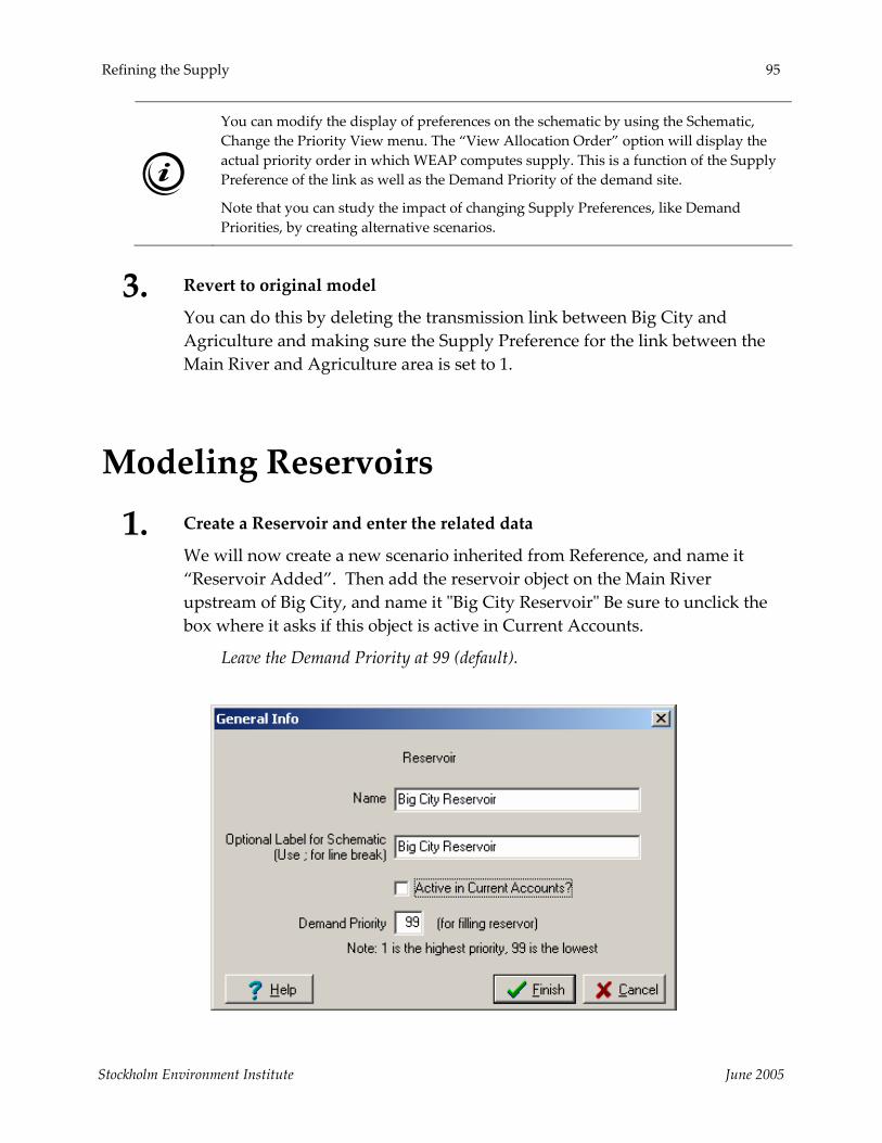
1. Create a Reservoir and enter the related data
We will now create a new scenario inherited from Reference, and name it “Reservoir Added”. Then add the reservoir object on the Main River upstream of Big City, and name it ʺBig City Reservoirʺ Be sure to unclick the box where it asks if this object is active in Current Accounts.
Leave the Demand Priority at 99 (default).
Stockholm Environment Institute June 2005

96 WEAP Tutorial
Right click on Big City Reservoir and select ʺEdit Dataʺ. (Make sure you have the “Reservoir Added” scenario selected). To alter parameters, you will first have to click on the “Startup Year” button.
Choose 2002 as the startup year for Big City Reservoir
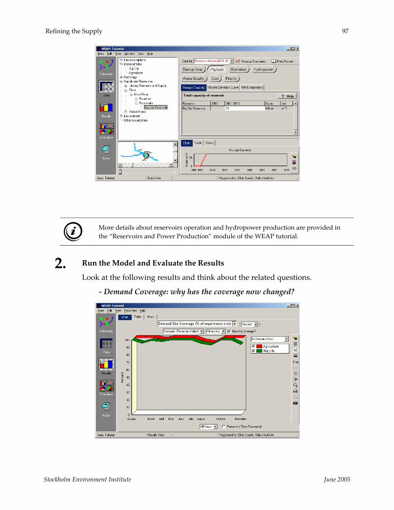
Then click on the “Physical” button and change the following parameters :
Storage Capacity 70 M m3 Note that the Scale is set to ʺMillionʺ
Stockholm Environment Institute June 2005
Refining the Supply 97
More details about reservoirs operation and hydropower production are provided in the “Reservoirs and Power Production” module of the WEAP tutorial.
2. Run the Model and Evaluate the Results
Look at the following results and think about the related questions.
‐ Demand Coverage: why has the coverage now changed?
Stockholm Environment Institute June 2005

98 WEAP Tutorial
‐ Reservoir Storage Volume: does the solution of building a reservoir appear to be sustainable? Use the Primary Variable pull down menu to select Reservoir Storage Volume, and select all years from the pull down menu at the bottom of the graph.
‐ Flow in the River: is the residual flow downstream of the reservoir adequate in the winter and spring? Select Streamflow from the Primary Variable pull down menu and click on Monthly Average.
Stockholm Environment Institute June 2005
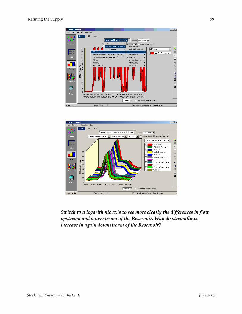
Refining the Supply 99
Switch to a logarithmic axis to see more clearly the differences in flow upstream and downstream of the Reservoir. Why do streamflows increase in again downstream of the Reservoir?
Stockholm Environment Institute June 2005

100 WEAP Tutorial
The creation of a large‐size reservoir allows storage of “excess” water during high flow periods to cover water demand during low flow periods. The price to pay is, however, a potentially large impact onto the hydrological regime of the river downstream of the reservoir. The Return Flows from Big City and Agriculture provide the flow in the Main River during the spring and winter months. A reservoir’s operation variables and flow requirements can be used to mitigate the reservoir’s downstream impact.
Stockholm Environment Institute June 2005

Refining the Supply 101
Adding Flow Requirements
1. Create a Flow Requirements
Create a Flow Requirement along the river in the city, downstream of the water withdrawal for the urban and agricultural demand sites.
Demand Priority 1 (default)
Right click on the Flow Requirement and select Edit Data/Minimal Flow Requirement. Add the value below (make sure you still have the “Reservoir Added” scenario selected):
Minimal Flow Requirement 5 CMS
Stockholm Environment Institute June 2005
102 WEAP Tutorial
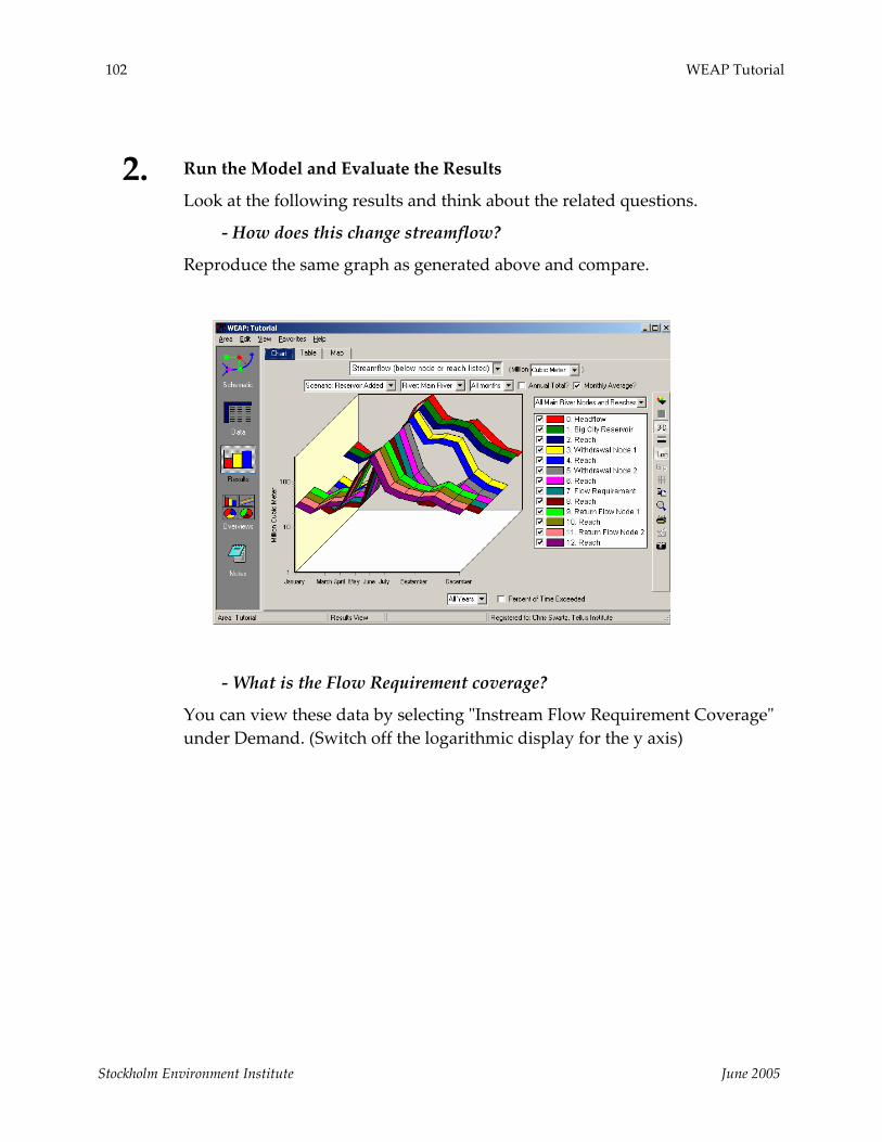
2. Run the Model and Evaluate the Results
Look at the following results and think about the related questions.
‐ How does this change streamflow?
Reproduce the same graph as generated above and compare.
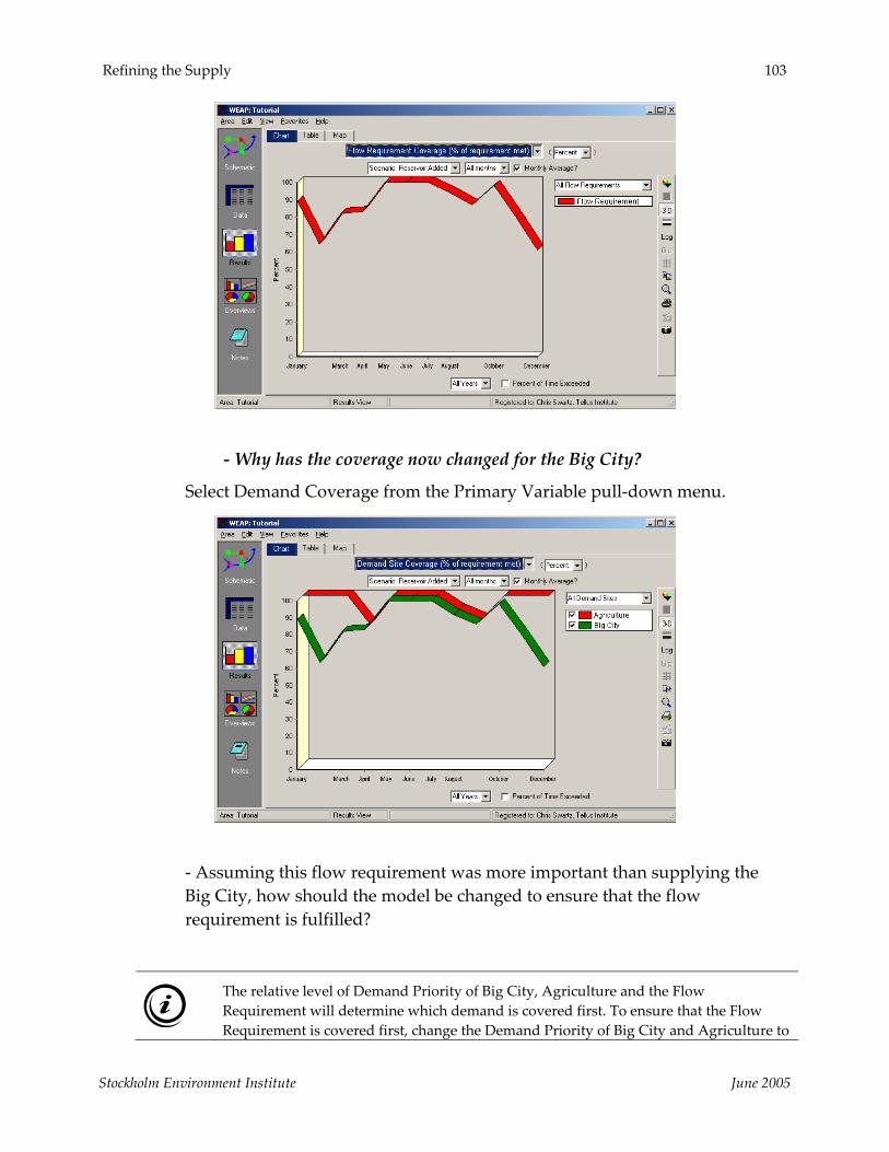
‐ What is the Flow Requirement coverage?
You can view these data by selecting ʺInstream Flow Requirement Coverageʺ under Demand. (Switch off the logarithmic display for the y axis)
Stockholm Environment Institute June 2005
Refining the Supply 103
‐ Why has the coverage now changed for the Big City?
Select Demand Coverage from the Primary Variable pull‐down menu.
‐ Assuming this flow requirement was more important than supplying the Big City, how should the model be changed to ensure that the flow requirement is fulfilled?
The relative level of Demand Priority of Big City, Agriculture and the Flow Requirement will determine which demand is covered first. To ensure that the Flow Requirement is covered first, change the Demand Priority of Big City and Agriculture to
Stockholm Environment Institute June 2005

104 WEAP Tutorial
a value higher than for the Flow Requirement. The Rural demand priority does not need to be changed since it is downstream of the Flow Requirement.
Modeling Groundwater Resources
1. Create a Groundwater Resource
Create a Groundwater Resource next to the City and name it ʺBig City Groundwaterʺ. Also, make it active in Current Accounts.
Give Big City Groundwater the following properties (make sure you are in Current Accounts when entering these data ‐ you will realize you are not if there is no tab for Initial Storage) :
Storage Capacity Unlimited (default, leave empty) Initial Storage 100M m3 Natural Recharge (use the Monthly Time Series Window, accessed in the field under ʺ2000ʺ) ‐ Nov. to Feb. 0M m3/month ‐ Mar. to Oct. 10M m3/month
Stockholm Environment Institute June 2005

Refining the Supply 105
2. Connect the Groundwater Field with Big City
Use a transmission link to connect the groundwater resources with the Big City demand site and provide a Supply Preference of 2. Your model should look similar to the figure below.
Stockholm Environment Institute June 2005

106 WEAP Tutorial
3. Update the characteristics of the link between Big City Reservoir and Big City
Change the characteristics of the transmission link connecting Big City Reservoir and Big City:
Supply Preference 1 (default) Maximum Flow Volume 13 m3/sec
The Maximum Flow Volume or Percent of Demand parameter models restrictions in the capacity of a resource (due, for example to equipment limits).
4. Run the Model and Evaluate the Results
Look at the following results and think about the related questions.
‐ Is the groundwater extraction sustainable?
To view these results, select Groundwater Storage from the pull‐down menu under Supply and Resources/Groundwater
Stockholm Environment Institute June 2005

Refining the Supply 107
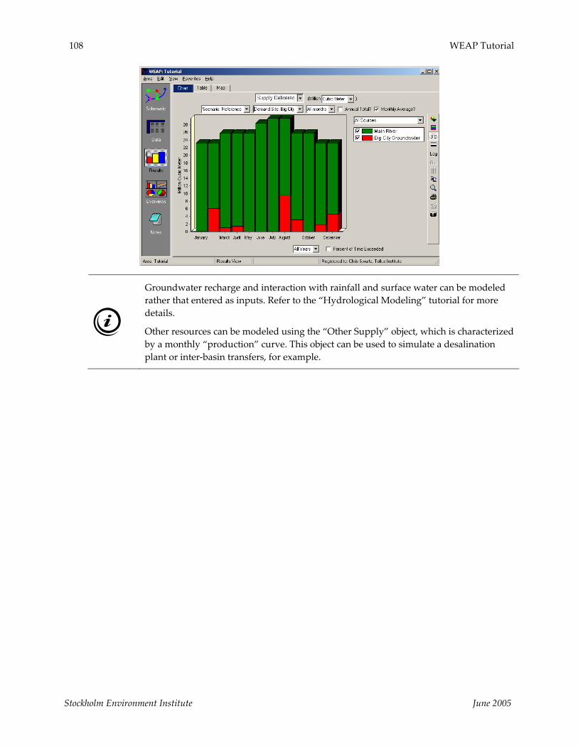
‐ How does the relative use of water from Big City Groundwater and the Main River evolve at the Big City demand site?
To view these graphical results for Big City specifically, first select ʺSupply Deliveredʺ under Demand within the Primary Variable pull‐down menu. Then choose ʺAll Sourcesʺ in the pull‐down menu on the right side of the window above the figure legend. Next, click on ʺSelected Demand Sitesʺ in the pull‐down menu centered above the graph and directly below primary variable field. Click OK.
Stockholm Environment Institute June 2005
108 WEAP Tutorial
Groundwater recharge and interaction with rainfall and surface water can be modeled rather that entered as inputs. Refer to the “Hydrological Modeling” tutorial for more details.
Other resources can be modeled using the “Other Supply” object, which is characterized by a monthly “production” curve. This object can be used to simulate a desalination plant or inter‐basin transfers, for example.
Stockholm Environment Institute June 2005

WEAP Water Evaluation And Planning System
Data, Results and Formatting
A TUTORIAL ON Exchanging Data ....................................................110
Importing Time Series ............................................113
Working with Results .............................................116
Formatting ..............................................................120
June 2005

110 WEAP Tutorial
Note: For this module you will need to have completed the previous modules (“WEAP in One Hour, Basic Tools, and Scenarios) or have a fair knowledge of WEAP (data structure, key assumptions, expression builder, creating scenarios). To begin this module, go to the Main Menu, select “Revert to Version” and choose the version named “Starting Point for all modules after ‘Scenarios’ module.”
Exchanging Data
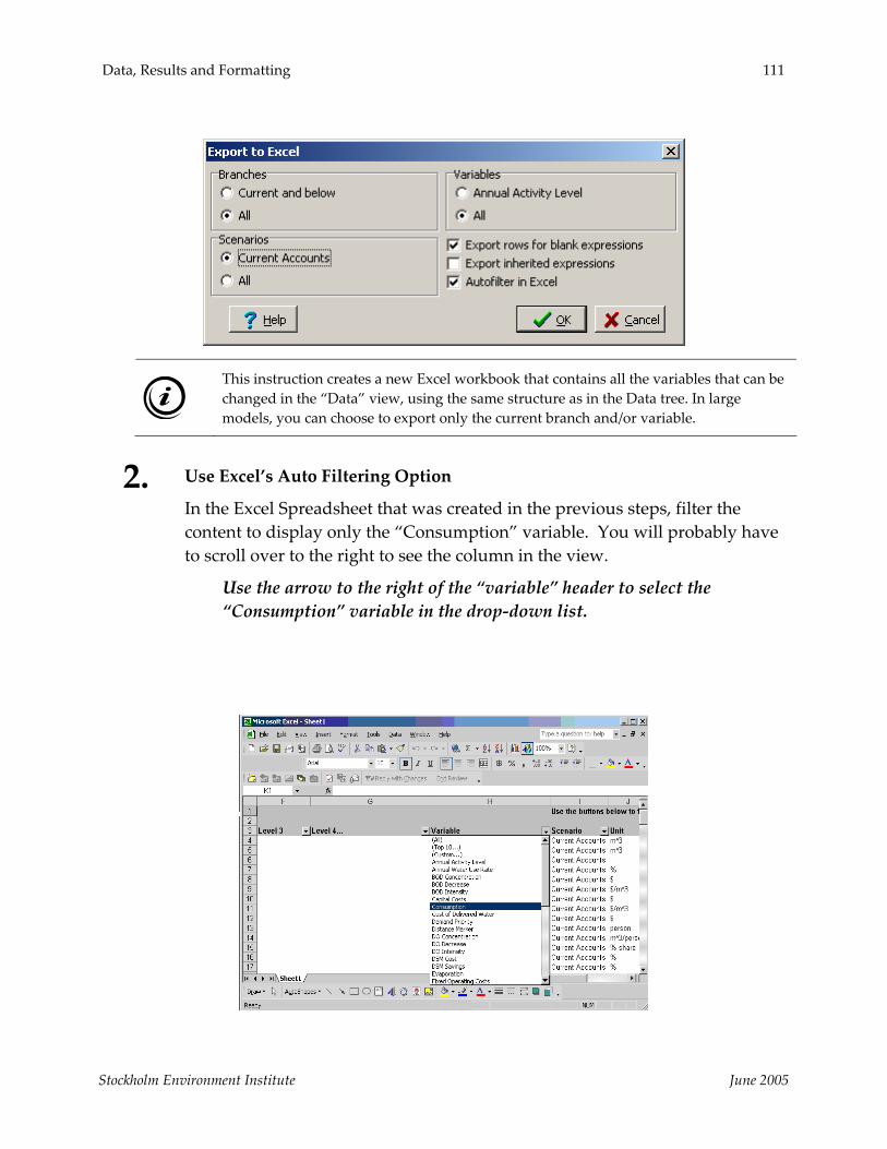
1. Export Data to Excel
Export the entire model to Excel by going to the Data view and selecting “Edit”, “Export to Excel”.
Export all branches, and all variables of the “Current Accounts” only (don’t export any of the scenarios for this example) to a new workbook. Keep other options at default values.
Stockholm Environment Institute June 2005
Data, Results and Formatting 111
This instruction creates a new Excel workbook that contains all the variables that can be changed in the “Data” view, using the same structure as in the Data tree. In large models, you can choose to export only the current branch and/or variable.
2. Use Excel’s Auto Filtering Option
In the Excel Spreadsheet that was created in the previous steps, filter the content to display only the “Consumption” variable. You will probably have to scroll over to the right to see the column in the view.
Use the arrow to the right of the “variable” header to select the “Consumption” variable in the drop‐down list.
Stockholm Environment Institute June 2005

112 WEAP Tutorial
Auto‐filtering does not change or erase the data; it only hides the rows that are not of interest. Multiple filters can be used.
3. Modify Data
In the Excel Spreadsheet that was created in the previous steps, make the following changes in the yellow column (it may be good to hide a few of the columns so that you can see both the variable values and the Demand Sites to which they belong in the same view):
Big City Consumption 5% (value was 15 originally) Agriculture Consumption 5% (value was 90 originally)
The values entered are not meant to be representative of realistic values, just examples.
When creating a large model, a quick way to enter a lot of data is to use the Excel Import and Export functions combined with the Excel lookup capabilities. This requires the user to have set up the model in a consistent way (data structure, names), however.
4. Import the Data from Excel
Re‐import the modified data in Excel.
In WEAP, choose “Edit”, “Import from Excel…” Check that the Consumption data have been changed in your model.
Stockholm Environment Institute June 2005

Data, Results and Formatting 113
WEAP always reads from the Excel file that had the focus last. If you have several Excel files open, you should ensure that the appropriate Excel file is selected before beginning the importation into WEAP.
When re‐importing into Excel, all rows are read, even those that are filtered out through the auto‐filtering options.
Importing Time Series
1. Create a Streamflow Gauge Object
Add a Streamflow Gauge object to the model.
Insert the streamflow gauge downstream of the Big City, below the return flow nodes for agriculture and the City supply.
Stockholm Environment Institute June 2005

114 WEAP Tutorial
2. Import Text File Data
Import stream flow data from a comma‐separated text file containing approximately 100 years of streamflow measurements up to 2003. To import the file, use the “ReadFromFile” function in the streamflow gauge’s data tab in the “Supply and Resources/River/Streamflow Gauges” branch of the Data tree.
Type in the following function, which will read the file from a directory called “Additional Files” located in your area’s folder. ”ReadFromFile(Additional Files\River_Flow.csv)”
The ReadFromFile function can be used for any variable that requires a time series, monthly or yearly, such as headflow, groundwater recharge, etc.
WEAP will automatically locate the correct year and month and only use that data. If
Stockholm Environment Institute June 2005

Data, Results and Formatting 115
you change the years modeled, WEAP will automatically read the correct data.
More information about the syntax of this function and the format of the data file can be found in the “Read from File” help topic.
3. Compare the Actual and Modeled Stream flow
Recalculate and compare the historical stream flow data with what WEAP simulates. Do this by clicking on the chart tab of the Results view and selecting from the pull‐down menu for the Primary Variable window: Supply and Resources/River/Streamflow Relative to Gauge (Absolute).
WEAP will compare the observed flow at the streamflow gauge to the nearest upstream node. In the case for this example, that node is Return Flow 2(the Return Flow for Agriculture). Comparing observed and simulated streamflow is one means for the user to assess if the model is representing the system accurately.
Choose the “Selected Years” option from the pull‐down menu above the chart legend and select only the years 2000, 2001, 2002, and 2003 (the Current Accounts is 2000, and there is no streamgauge data beyond 2003). The Reference scenario will automatically be displayed when you choose the “Selected Years” option. You should obtain the graph below:
Stockholm Environment Institute June 2005

116 WEAP Tutorial
Notice that the simulated streamflow is greater than the observed streamflow in the Current Accounts year (2000), but falls to less than observed in subsequent years.
Working with Results
1. Create a Favorite Graph
Create a graph of streamflow that shows both the actual flow as recorded at the streamgauge and the simulated streamflow at the appropriate node upstream of the streamgauge (in this example, Return Flow Node 2). First, select Streamflow from the Primary Variable pull‐down menu. Then select Streamgauge and Below Return Flow Node 2 from the list that appears when you choose “Select Nodes and Reaches…” in the drop down menu of the Supply and Resources/River/Streamflow chart above the graph legend (see below). Finally, select the years 2000, 2001, 2002, and 2003 to be represented in the graph using the pull‐down menu at the bottom of the window.
Save this graph as a favorite by using the “Favorite”, “Save Chart as Favorite” option. Name the file ʺSimulated and Observed Streamflow Comparisonʺ.
Stockholm Environment Institute June 2005

Data, Results and Formatting 117
From this point forward, the chart will appear in the list of favorite charts of the Results view.
You can also export the data to Excel or to the clipboard, change the format and the display of figures and charts, calculate statistics, group series with the smallest values, etc. from the toolbar located at the right of the “Results” view.
2. Create an Overview
Create an overview displaying the streamflow, inflow, and outflow to area charts.
Select the “Overview” view. Under “Manage Overviews”, select “Inflows to area”, “Outflows to area” and the Favorite graph created in the previous step.
Stockholm Environment Institute June 2005

118 WEAP Tutorial
Overviews can be created from any combination of favorites, but the charts need to be created in the “Results” view prior to their integration in an overview. The data underlying overviews can also be displayed in tabular format (select the “Table” tab) and exported to Excel.
3. Use the Dynamic Map
Dynamic Results Maps are a quick way to obtain an overview of the results in their temporal context. In the “Results” view, select the “Map” tab and play with the time slider at the bottom of the display to see how the displayed parameters change.
Try this by selecting the Main River’s streamflow.
Note that as you pull the slider across the bar, an indicator appears in the graph above the bar to indicate the data selected (for this example, the year
Stockholm Environment Institute June 2005

Data, Results and Formatting 119
2004 annual total is selected). In the smaller schematic view at the top of the window, the width of the river will increase and decrease with the changing data, and numerical values appear for each of the reaches.
4. Export Results to Excel
All results can be readily exported to Excel from the “Results” view. A new workbook is created that contains the results in table format, with the same structure as in WEAP.
Recall the favorite graph you have created a few steps before by selecting it in the “Favorite” menu of the Results View. Export the related data to Excel by switching to the “Table” tab and hitting the “Export Table to Excel” button ( ) to the right of the screen.
5. Calculate Statistics
You can generate statistics in the Results view for any table. Just click on the Table tab and then click on the ʺStatʺ icon on the right vertical menu bar.
Stockholm Environment Institute June 2005

120 WEAP Tutorial
Formatting
1. Change the Appearance of a Background Vector Layer
In the Schematic View, change the color of the Big City by right‐clicking the “Cities” layer in the box below the Element Selection box (see example below), and selecting “Edit…”. Click on the Appearances tab, then click on the Fill Color field. A color palette will appear.
Change the Background color to orange.
Stockholm Environment Institute June 2005
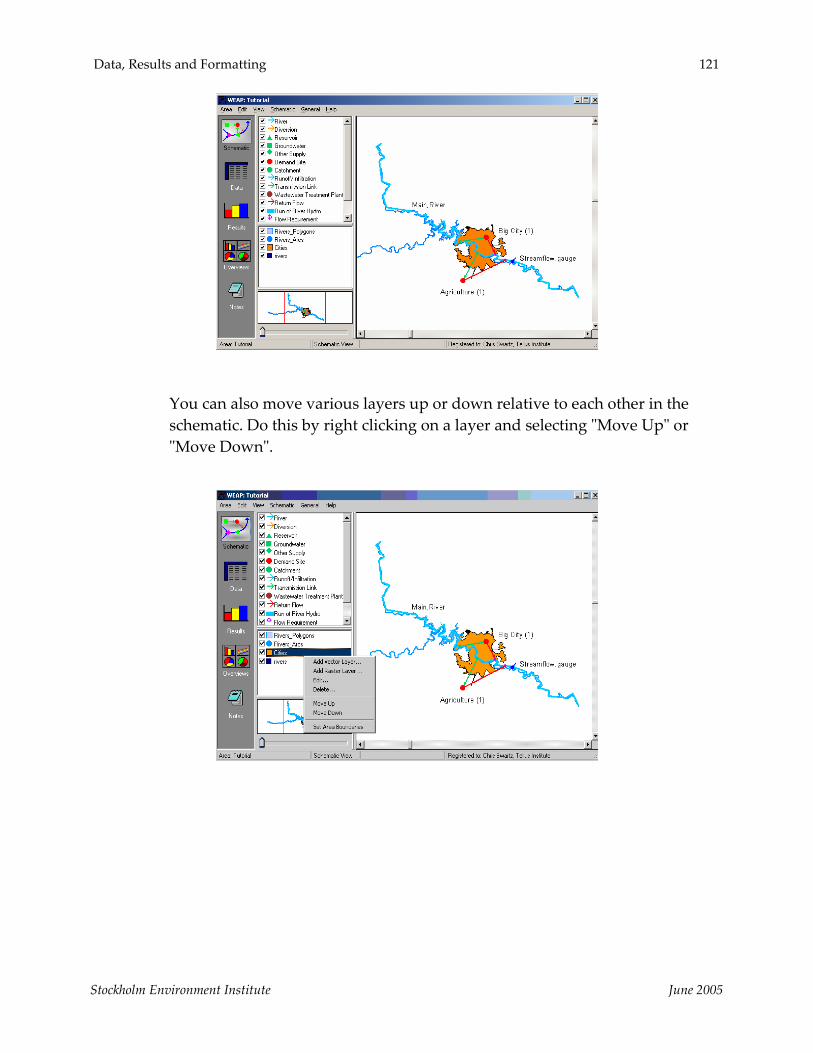
Data, Results and Formatting 121
You can also move various layers up or down relative to each other in the schematic. Do this by right clicking on a layer and selecting ʺMove Upʺ or ʺMove Downʺ.
Stockholm Environment Institute June 2005
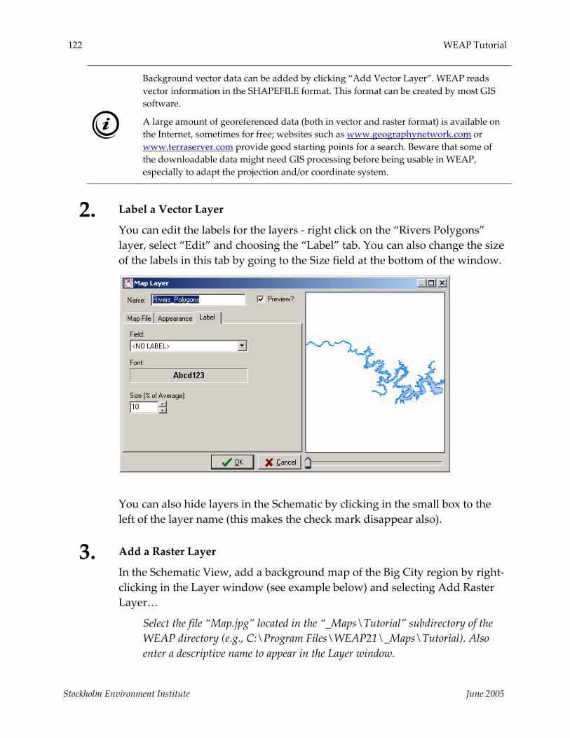
122 WEAP Tutorial
Background vector data can be added by clicking “Add Vector Layer”. WEAP reads vector information in the SHAPEFILE format. This format can be created by most GIS software.
A large amount of georeferenced data (both in vector and raster format) is available on the Internet, sometimes for free; websites such as www.geographynetwork.com or www.terraserver.com provide good starting points for a search. Beware that some of the downloadable data might need GIS processing before being usable in WEAP, especially to adapt the projection and/or coordinate system.
2. Label a Vector Layer
You can edit the labels for the layers ‐ right click on the “Rivers Polygons” layer, select “Edit” and choosing the “Label” tab. You can also change the size of the labels in this tab by going to the Size field at the bottom of the window.
You can also hide layers in the Schematic by clicking in the small box to the left of the layer name (this makes the check mark disappear also).
3. Add a Raster Layer
In the Schematic View, add a background map of the Big City region by right‐clicking in the Layer window (see example below) and selecting Add Raster Layer…
Select the file “Map.jpg” located in the “_Maps\Tutorial” subdirectory of the WEAP directory (e.g., C:\Program Files\WEAP21\_Maps\Tutorial). Also enter a descriptive name to appear in the Layer window.
Stockholm Environment Institute June 2005

Data, Results and Formatting 123
Stockholm Environment Institute June 2005
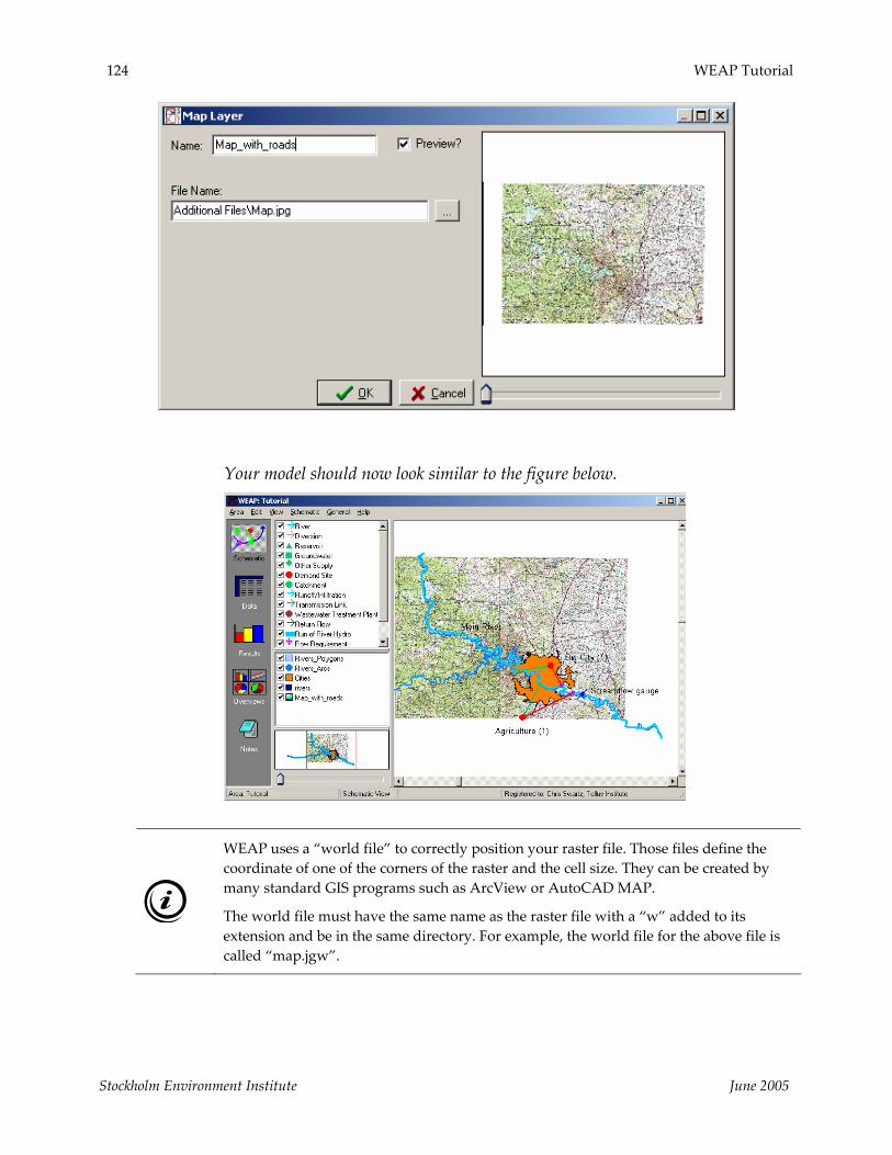
124 WEAP Tutorial
Your model should now look similar to the figure below.
WEAP uses a “world file” to correctly position your raster file. Those files define the coordinate of one of the corners of the raster and the cell size. They can be created by many standard GIS programs such as ArcView or AutoCAD MAP.
The world file must have the same name as the raster file with a “w” added to its extension and be in the same directory. For example, the world file for the above file is called “map.jgw”.
Stockholm Environment Institute June 2005

Data, Results and Formatting 125
4. Move around Labels
Complete the formatting of your area by changing the node and label font size and moving around labels.
Use the Schematic, Set WEAP Node Size and Set WEAP Node Label Size menu to change the size of symbols and labels. For each of these actions, a window with a slider will appear for increasing and decreasing the size of these elements.
Stockholm Environment Institute June 2005

126 WEAP Tutorial
Right‐Click on any object and select “Move Label” to move its label.
If you don’t want a label to appear for a given object, just right‐click that object, select “General Info” and delete the optional label text.
You can copy your map to the clipboard for later use in reports and presentations by selecting “Copy Schematic to Clipboard…” in the “Schematic” menu. The file size indicated in the dialog box corresponds to an uncompressed format. It is usually safe to go with the default level of detail.
Stockholm Environment Institute June 2005
WEAP Water Evaluation And Planning System
Reservoirs and Power Production
A TUTORIAL ON Modeling Reservoirs ...............................................128
Adding Hydropower Computation.........................133
Modeling Run‐of‐River Power Plants....................135
June 2005

128 WEAP Tutorial
Note: For this module you will need to have completed the previous modules (“WEAP in One Hour, Basic Tools, and Scenarios) or have a fair knowledge of WEAP (data structure, key assumptions, expression builder, creating scenarios). To begin this module, go to the Main Menu, select “Revert to Version” and choose the version named “Starting Point for all modules after ‘Scenarios’ module.”
Modeling Reservoirs
1. Create a Reservoir
Create a Reservoir on the Lake located upstream of the Big City. Name it Big City Reservoir
Demand Priority 99 (default)
Entering a Demand Priority of 99 ensures that the reservoir will only fill if all other needs are fulfilled, including downstream demand.
2. Enter the Physical Data
Right click on Big City Reservoir to edit data. Enter the following data in the “Physical” window.
Storage Capacity 70 M m3 Initial Storage 25 M m3 Volume Elevation Curve Volume Elevation M m3 m 0.0 190 30.0 210 70.0 216 Net Evaporation 25 mm/month.
Stockholm Environment Institute June 2005

Reservoirs and Power Production 129
The Volume Elevation Curve is used both to model the surface for evaporation and to compute the head in case hydropower production is simulated. A cylindrical shape is assumed in converting volume and elevation into area.
Net evaporation needs to account for both rainfall and evaporation. It can therefore be a positive or a negative number; monthly variations can be modeled using the “Monthly Time Series Wizard”.
3. Enter the Operation Data
In the same view, enter the following data in the “Operation” window.
Stockholm Environment Institute June 2005

130 WEAP Tutorial
Top of Conservation 60 Top of Buffer 40 Top of Inactive 5 Buffer Coefficient 1.0
As illustrated by the figure to the left, WEAP allows the modeling of advanced reservoir operation through the definition of several zones that have different operational constraints.
More can be learned through the Help file’s “Reservoir Zones and Operation” screen or by clicking on the help button when in the Reservoir’s Operation tab.
4. Understanding the Impact of the Buffer Coefficient
Run the Model as is, then again with a buffer coefficient of 0.1 and compare the results for Reservoir Storage Volume, found under the Supply and Resources/Reservoirs branch of the Primary Variable pull‐down menu. Do this for all months of the year 2000 by selecting this year on the pull‐down menu at the bottom of the graph, and choose the Reference scenario for viewing from the pull‐down menu below the Primary Variable pull‐down
Stockholm Environment Institute June 2005

Reservoirs and Power Production 131
menu at the top of the graph. You can choose “All Reservoirs” from the pull‐down menu above the graph legend.
Reservoir Storage Volume; Buffer Coefficient = 1
Reservoir Storage Volume; Buffer coefficient = 0.1
Compare results also for Demand Coverage (under the Demand branch). For this graph, you can select “All Demand Sites” for viewing from the pull‐down menu above the graph legend.
Stockholm Environment Institute June 2005

132 WEAP Tutorial
Demand Coverage; Buffer coefficient = 1
Demand Coverage; Buffer coefficient = 0.1
Afterward, set the buffer coefficient back at 1.
Stockholm Environment Institute June 2005

Reservoirs and Power Production 133
The buffer coefficient provides a way to regulate water releases when the water level in the reservoir is within the buffer zone (see figure in the information box of the previous step). The downstream demand is multiplied by the buffer coefficient to obtain actual water release. Thus a buffer coefficient of 1 means that as much water is released as is needed to cover downstream demand (in other terms, the buffer zone is a mere extension of the conservation zone). A coefficient of 0 means no water is released.
Adding Hydropower Computation
1. Understanding the way WEAP models Power Production
WEAP can model Power Production in three different ways: through on‐line reservoirs, through off‐line reservoirs, and through run‐of‐river hydropower plants.
Refer to the help for more information on each category.
2. Add Power Production Capabilities to the Reservoir
In this example we will model an on‐line reservoir power plant. Enter the following data under the Hydropower window for Big City Reservoir.
Min Turbine Flow 5 CMS Max Turbine Flow 80 CMS Tailwater Elevation 195m Plant Factor 100% Generating Efficiency 60%
Stockholm Environment Institute June 2005

134 WEAP Tutorial
Look at the “Hydropower Calculations” help topic for more information about how WEAP computes power production.
3. Compute Hydropower Production and Understand the Results
Run the model and look at the results in terms of power production for the year 2000.
The results can be accessed under the Primary Variable pull‐down menu under “Supply and Resources/Reservoir/Hydropower”.
Stockholm Environment Institute June 2005
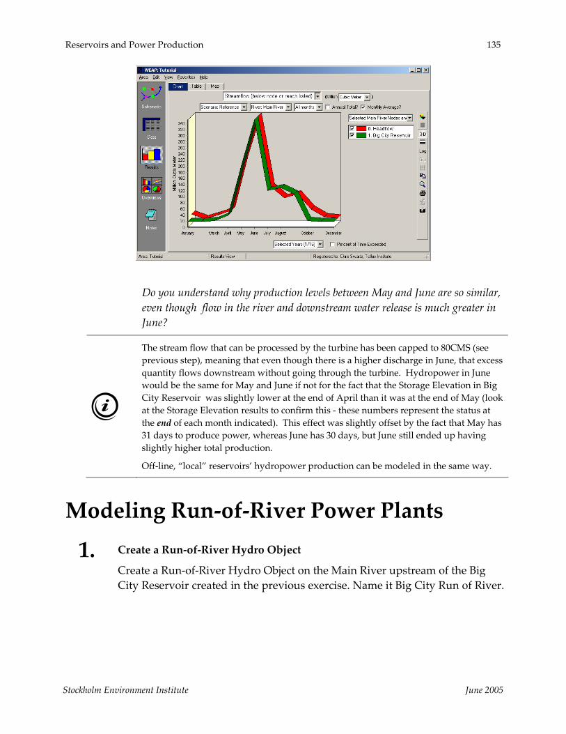
Reservoirs and Power Production 135
Do you understand why production levels between May and June are so similar, even though flow in the river and downstream water release is much greater in June?
The stream flow that can be processed by the turbine has been capped to 80CMS (see previous step), meaning that even though there is a higher discharge in June, that excess quantity flows downstream without going through the turbine. Hydropower in June would be the same for May and June if not for the fact that the Storage Elevation in Big City Reservoir was slightly lower at the end of April than it was at the end of May (look at the Storage Elevation results to confirm this ‐ these numbers represent the status at the end of each month indicated). This effect was slightly offset by the fact that May has 31 days to produce power, whereas June has 30 days, but June still ended up having slightly higher total production.
Off‐line, “local” reservoirs’ hydropower production can be modeled in the same way.
Modeling Run‐of‐River Power Plants
1. Create a Run‐of‐River Hydro Object
Create a Run‐of‐River Hydro Object on the Main River upstream of the Big City Reservoir created in the previous exercise. Name it Big City Run of River.
Stockholm Environment Institute June 2005

136 WEAP Tutorial
Enter the following data in the Supply and Resources/River/Run of River Hydro branch of the Data tree in the Data View :
Min Turbine Flow 5 CMS Max Turbine Flow 80 CMS Plant Factor 100% Generating Efficiency 60% Fixed Head 19.5 m
Stockholm Environment Institute June 2005

Reservoirs and Power Production 137
2. Run and Compare Results
Run your model and create a graph comparing the power production for the run‐of‐river and the reservoir power plants. Do this by selecting “All Hydropower” from the pull‐down menu above the legend.
What are the reasons for the differences between both curves?
Note that the Run of River hydropower is slightly higher in May than June, in contrast to Big City Reservoir power production. This is due to the additional day available in May compared to June. Run of River hydropower production does not have Storage Elevation as limiting effect, whereas the Reservoir was still filling in May, which decrease the Reservoir production for that month compared to June.
Stockholm Environment Institute June 2005
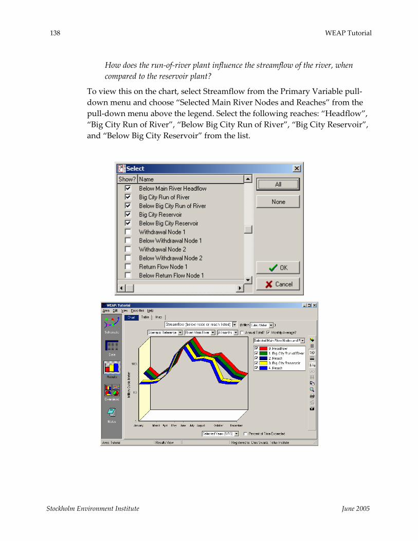
138 WEAP Tutorial
How does the run‐of‐river plant influence the streamflow of the river, when compared to the reservoir plant?
To view this on the chart, select Streamflow from the Primary Variable pull‐down menu and choose “Selected Main River Nodes and Reaches” from the pull‐down menu above the legend. Select the following reaches: “Headflow”, “Big City Run of River”, “Below Big City Run of River”, “Big City Reservoir”, and “Below Big City Reservoir” from the list.
Stockholm Environment Institute June 2005

Reservoirs and Power Production 139
While a reservoir can store water during high flows and release during low flow, thus having a smoothing effect, a run‐of‐river only processes whatever water flows in the river at any given point in time. Therefore, it does not affect the shape of the streamflow curve.
Stockholm Environment Institute June 2005


WEAP Water Evaluation And Planning System
Water Quality
A TUTORIAL ON Setting up Quality Modeling .................................142
Entering Water Quality Data.................................144
Modeling a Wastewater Treatment Plant ..............152
June 2005

142 WEAP Tutorial
Note: For this module you will need to have completed the previous modules (“WEAP in One Hour, Basic Tools, and Scenarios) or have a fair knowledge of WEAP (data structure, key assumptions, expression builder, creating scenarios). To begin this module, go to the Main Menu, select “Revert to Version” and choose the version named “Starting Point for all modules after ‘Scenarios’ module.”
Setting up Quality Modeling
1. Understanding Water Quality Modeling in WEAP
WEAP can model both conservative and non‐conservative point pollutants. Conservative pollutants are modeled through a simple mass balance. Several models are offered for non‐conservative pollutants.
Read the Environment Overview help topic for a more detailed description of WEAP capabilities.
2. Create a Set of Pollutants
Create a set of pollutants that will be modeled by going to the “General”, “Water Quality Constituents” menu. In the dialog box, make the following change and create the following pollutants:
Name Calculate by Decay Rate Temperature Change to “modeled” TSS Decay 0.25 per day Salt Conservative
Stockholm Environment Institute June 2005

Water Quality 143
Stockholm Environment Institute June 2005

144 WEAP Tutorial
More details are provided on the different models used for BOD and DO models in the “Dissolved Oxygen and Biochemical Oxygen Demand” help topic.
Entering Water Quality Data
1. Enter River Water Quality data
In the Data view’s tree, select “Supply and Resources”, “River” and click on your river. Then open the “Water Quality” screen and enter the following data, which will represent water quality at the headflow of the river.
Model Water Quality? YES (check the box) Temperature 15°C
Stockholm Environment Institute June 2005

Water Quality 145
BOD concentration 5mg/l DO Concentration 8mg/l TSS concentration 20mg/l Salt concentration 2mg/l
2. Enter River Geometric Characteristics
River geometric characteristics are needed for the various water quality models. They are mainly used to compute velocity / residence time of the water. In the same view as in the previous step, select the “Reaches” branch
Stockholm Environment Institute June 2005

146 WEAP Tutorial
of your river and enter the following information under the “Water Quality” tabs.
Headflow Distance Marker 0 km Tailflow Distance Marker 300 km Note: intermediate reach lengths will be estimated by WEAP based on the schematic.
Flow Stage Width for the headflow reach (use the Wizard by clicking on the drop‐down arrow) Flow Stage Width 0 0.00 0.00 10 2.00 15.00 50 6.00 20.00 100 8.00 25.00 200 10.00 30.00 Your final formula should read: FlowStageWidthCurve( 0, 0, 0, 10, 2, 15, 50, 6, 20, 100, 8, 25, 200, 10, 30 ) We will assume this section remains constant and leave other reaches empty.
Stockholm Environment Institute June 2005

Water Quality 147
Stockholm Environment Institute June 2005
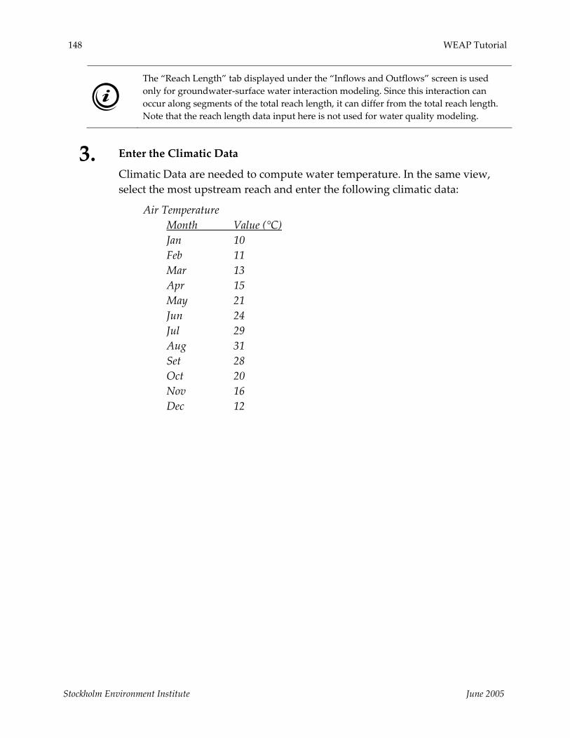
148 WEAP Tutorial
The “Reach Length” tab displayed under the “Inflows and Outflows” screen is used only for groundwater‐surface water interaction modeling. Since this interaction can occur along segments of the total reach length, it can differ from the total reach length. Note that the reach length data input here is not used for water quality modeling.
3. Enter the Climatic Data
Climatic Data are needed to compute water temperature. In the same view, select the most upstream reach and enter the following climatic data:
Air Temperature Month Value (°C) Jan 10 Feb 11 Mar 13 Apr 15 May 21 Jun 24 Jul 29 Aug 31 Set 28 Oct 20 Nov 16 Dec 12
Stockholm Environment Institute June 2005

Water Quality 149
Humidity 65% Wind 1 m/s Latitude 30°
Note: you can enter these values for the first reach and leave the other reaches blank if you want the value to apply to all reaches.
Stockholm Environment Institute June 2005

150 WEAP Tutorial
4. Enter Pollution Generation Activities for the Big City
For Big City we will assume we know the concentration of pollutants in the outflow of the City. Hence we will use the “Concentration” series of tabs in the Environment, Pollutant Generation, Big City branch of the Data tree. Enter the following data:
Temperature 16 °C BOD Concentration 60 mg/l DO Concentration 3 mg/l TSS Concentration 5 mg/l Salt Concentration 10 mg/l
5. Enter Pollution Generation Activities for the Agriculture Area
For the agriculture area we will admit that we do not know the concentration at the outflow, but we do know the pollutant generation intensity. Enter the following data:
Annual Activity Level 100,000 ha (create a link to the Demand Site data) BOD intensity 50 kg/ha DO Intensity 30 kg/ha TSS Intensity 20 kg/ha Salt Intensity 2 kg/ha Temperature 15°C
Stockholm Environment Institute June 2005

Water Quality 151
Inputting data for pollutant generation, using either model, will cause WEAP to disregard the pollutant concentration in the inflow to the demand site.
6. Evaluate the Results
Run the model and look at the following results for the various pollutants. All the water quality‐related results are displayed under the “Environment” category.
Demand Site Pollution Generation Surface Water Quality
Stockholm Environment Institute June 2005

152 WEAP Tutorial
Note that the pollution generation for Agriculture is constrained to the spring and summer months when farming is active.
Modeling a Wastewater Treatment Plant
1. Create a Wastewater Treatment Plant
Create a new scenario named “Wastewater Treatment Plant Added”‐ this scenario inherited from the Reference. Then, add a Wastewater Treatment Plant for Big City (make it inactive in Current Accounts), and create another Return flow link from the Big City to the WWTP. Keep the existing Return Flow Link from Big City to the river. Also create a return flow from the WWTP to the river. Your model should look similar to the figure below.
You will have to set the Return Flow Routing variables for both link.
For the Return Flow from Big City to Return Flow Node 1, set this variable to 100% for the Current Accounts year and 0% for years 2001‐2015 in the “Wastewater Treatment Plant Added” scenario. For the Return Flows from Big City WWTP, set the Return Flow to 100% for the Current Accounts year and the years 2001‐2015 even though flow is not passing through the WWTP in the Current Accounts year (Return Flow Routing for any Return Flow Link must always sum to 100%)
Stockholm Environment Institute June 2005

Water Quality 153
You also have the possibility to set removal rates in the various return flows. This would be useful if, for example, a given pollutant is decomposed by bacteria in the sewer system. Enter the appropriate data in the Environment, Pollutant Decrease in Return Flows branch of the data tree.
2. Enter WWTP Data
First, enter the Start Year by clicking on the “Start Year” window under the Environment/Wastewater Treatment branch of the data tree for Big City WWTP.
Stockholm Environment Institute June 2005

154 WEAP Tutorial
Start Year 2001
Also enter the following data in the “Treatment” window (with the “Wastewater Treatment Plant Added” scenario selected:
Consumption 5% Daily Capacity 2M m3 BOD Removal 90% DO Concentration 5mg/l TSS Removal 80% Salt Removal 20% Temperature 15°C (reference to Big City demand site)
Stockholm Environment Institute June 2005

Water Quality 155
If only part of the wastewater is treated through the WWTP, there are two modeling possibilities. One is to limit the Daily Capacity to whatever amount can actually be treated. In this case the wastewater in excess will be discharged without treatment. The share of untreated wastewater is not constant, but depends on the total flow. Another solution is to create an additional return flow going from the demand site straight to the river, by‐passing the WWTP. In this case, a constant share can be set to by‐pass the WWTP by setting the return flow routing shares accordingly. A combination of both methods is also possible.
3. Evaluate the Results
Run the model and look at the following results for BOD in the “Wastewater Treatment Plant Added” scenario, comparing them with the Reference scenario values without a wastewater treatment plant.
Surface Water Quality (BOD downstream of Big City’s outflow into the river).
To view these results, first select “Surface Water Quality” under “Environment” in the Primary Variable pull‐down menu. Then choose “Selected Scenarios” under the pull‐down menu above the chart legend and select the “Reference” and “Wastewater Treatment Plant Added” scenarios. Using the pull‐down menu at the bottom of the chart, select the years 2000 and 2001 for viewing. Select “Below Return Flow Node 3” (Return Flow Node 3 is the return flow for the WWTP, so you will be looking at water quality in the river just downstream of the outflow from the WWT) as the Main River reach to view and BOD as the water quality constituent from the two pull‐
Stockholm Environment Institute June 2005
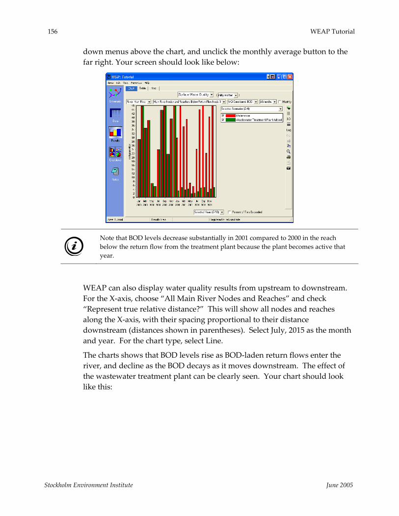
156 WEAP Tutorial
down menus above the chart, and unclick the monthly average button to the far right. Your screen should look like below:
Note that BOD levels decrease substantially in 2001 compared to 2000 in the reach below the return flow from the treatment plant because the plant becomes active that year.
WEAP can also display water quality results from upstream to downstream. For the X‐axis, choose “All Main River Nodes and Reaches” and check “Represent true relative distance?” This will show all nodes and reaches along the X‐axis, with their spacing proportional to their distance downstream (distances shown in parentheses). Select July, 2015 as the month and year. For the chart type, select Line.
The charts shows that BOD levels rise as BOD‐laden return flows enter the river, and decline as the BOD decays as it moves downstream. The effect of the wastewater treatment plant can be clearly seen. Your chart should look like this:
Stockholm Environment Institute June 2005

Water Quality 157
Wastewater Treatment Plant Inflows and Outflows.
To view these results, select the “Wastewater Treatment Plant Inflows and Outflows” from the Primary Variable pull‐down menu.
In this type of chart, the outflows are represented as negative values and inflows are positive values. Note also that the “Lost in Treatment” category represents the flow that is consumed ‐ a consumption rate of 5% was input in the data view for the treatment plant.
Stockholm Environment Institute June 2005

158 WEAP Tutorial
Stockholm Environment Institute June 2005

WEAP Water Evaluation And Planning System
Hydrology
A TUTORIAL ON Modeling Catchments: the Rainfall Runoff Model ......................................................................160
Modeling Catchments: the Soil Moisture Model ......................................................................165
Simulating Surface Water‐Groundwater Interaction...............................................................170
June 2005

160 WEAP Tutorial
Note: For this module you will need to have completed the previous modules (“WEAP in One Hour, Basic Tools, and Scenarios) or have a fair knowledge of WEAP (data structure, key assumptions, expression builder, creating scenarios). To begin this module, go to the Main Menu, select “Revert to Version” and choose the version named “Starting Point for all modules after ‘Scenarios’ module.”
Modeling Catchments: the Rainfall Runoff Model
1. Create a New Catchment
Create a Catchment object in the Schematic View to model the headflow of big river. Do this by pulling over a catchment node and locating it near the starting point of the Main River. Name it “Main River Headflow”. Once positioned, a dialog box will open and request the following data:
Runoff to Main River Represents Headflow Yes (check box) Infiltration to No inflow to GW Includes Irrigated Areas No (Default) Demand Priority 1 (default)
Note that when you have finished creating the Catchment node, a dashed blue line will automatically appear in the schematic linking the node to the Main River.
Stockholm Environment Institute June 2005

The Rainfall Runoff (Soil Moisture) Model 161
2. Create an Appropriate Substructure in the Basin
In the Data tree of the Data View, enter the following data. When first selecting the catchment to enter data, select the “Rainfall Runoff (FAO)” method under the “Advanced” tab.
Stockholm Environment Institute June 2005

162 WEAP Tutorial
Area 10M ha (you will have to choose the units first) Effective Prec. 98% Irrigated? 0 (1 indicates irrigation, 0 not) Crop Coefficients (use the Monthly Time Series Wizard to input these data) Sep to Feb 0.9 March 1.0 April 1.1 May 1.4 Jun to Aug 1.1
Stockholm Environment Institute June 2005
The Rainfall Runoff (Soil Moisture) Model 163
The Rainfall Runoff method is a simple method that computes runoff as the difference between precipitation and plant’s evapotranspiration. A portion of the precipitation can be set to bypass the evapotranspiration process and go straight into runoff to ensure a base flow (through the “effective precipitation” parameter).
The evapotranspiration is estimated by first entering the reference evapotranspiration, then defining crop coefficients for each type of land use (Kc’s) that multiply the reference evapotranspiration to reflect differences occurring from plant to plant.
More information about this method can be obtained from the FAO Irrigation and Drainage Paper 56, called “Crop Evapotranspiration” and available from the FAO’s website (www.fao.org).
Entering an effective precipitation other than 100% is one way of acknowledging the fact that part of the rainfall is not submitted to evapotranspiration during high intensity rainfall events, hence generating a minimal runoff to the river even when the rainfall is lower than the potential evapotranspiration. Another solution is to move to more developed models such as the 2‐buckets soil moisture model coupled with Surface Water – Groundwater interaction modeling, as presented later in this module.
3. Enter the Climatic Data
Climatic Data are entered at the catchment level. In the Data View, select the new catchment under the ”Demand Sites and Catchments” branch of the data tree and enter the following data under the “Climate” tab using the Monthly Time Series Wizard :
Month Precip. ETref Jan 21 42 Feb 37 47 Mar 56 78 Apr 78 86 May 141 131 Jun 114 122 Jul 116 158 Aug 85 140 Sep 69 104 Oct 36 79 Nov 22 43 Dec 13 37
Stockholm Environment Institute June 2005

164 WEAP Tutorial
If not available from on‐site stations, precipitation data can sometimes be derived from world‐wide climate models such as the one developed by Tim Mitchell at the University of East Anglia (http://www.cru.uea.ac.uk/~timm/data/index.html). The use of GIS software to extract the appropriate data is required. Such models provide average data in opposition to actual data, implying that the calibration is much more delicate.
The Reference Evapotranspiration can be determined from a set of climatic and topographic parameters using the Penman‐Monteith equation. More details are provided in the FAO publication mentioned earlier. Also, there exist global models of monthly reference evapotranspiration put together by the FAO, available from the FAO’s website.
4. Look at First Results
Results for Catchments are located in the “Catchment” category in the Primary Variable pull‐down menu.
Runoff from Precipitation to the Main River should look similar to the figure below. Select the Reference scenario from the pull‐down menu above the graph legend and Main River Headflow from the pull‐down menu above the graph
Stockholm Environment Institute June 2005
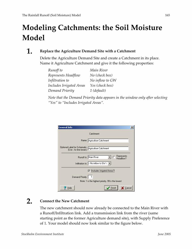
The Rainfall Runoff (Soil Moisture) Model 165
Modeling Catchments: the Soil Moisture Model
1. Replace the Agriculture Demand Site with a Catchment
Delete the Agriculture Demand Site and create a Catchment in its place. Name it Agriculture Catchment and give it the following properties:
Runoff to Main River Represents Headflow No (check box) Infiltration to No inflow to GW Includes Irrigated Areas Yes (check box) Demand Priority 1 (default)
Note that the Demand Priority data appears in the window only after selecting “Yes” to “Includes Irrigated Areas”.
2. Connect the New Catchment
The new catchment should now already be connected to the Main River with a Runoff/Infiltration link. Add a transmission link from the river (same starting point as the former Agriculture demand site), with Supply Preference of 1. Your model should now look similar to the figure below.
Stockholm Environment Institute June 2005

166 WEAP Tutorial
The purpose of this transmission link is to allow supplying irrigated areas with water from the river in case rainfall is insufficient.
3. Create sub‐structure in the Catchment
We will assume this catchment has three types of land use. In the Data View, add the following branches to your new catchment by right‐clicking it in the data tree and selecting “Add”. (If you select the catchment for editing by right clicking on the node in the schematic view rather than going through the data view, you will be asked beforehand to choose a simulation method ‐ pick the “Rainfall Runoff (soil moisture model)” method).
Irrigated Forest Grasslands
4. Enter the Appropriate Land Use Data
If you have not done so already, select the newly created Catchment in the Data view and pick the “Rainfall Runoff (soil moisture model)” method by clicking on the “Advanced” button. Then enter the following data after clicking on the “Land Use” button:
Total Land Area 300,000 ha (you will have to select units first) Irrigated Forest Grasslands Share of Land Area 33% 25% remainder(100)
Stockholm Environment Institute June 2005

The Rainfall Runoff (Soil Moisture) Model 167
Irrigated Forest Grasslands Leaf Area Index 3.6 3.0 1.7 Root Zone Conductivity 60 35 45 mm/month Preferred Flow Dir. 0.15 0.15 0.15 Initial Z1 50% 20% 20%
The remaining variables are the same for all land classes in the catchment:
Initial Z2 20% Root Zone Water Capacity 900 mm Deep Water Capacity 35,000 mm Deep Conductivity 240 mm/month Kc Use the same values as input for the Main River Headflow catchment in the previous exercise. You can simply copy and paste that expression into the Kc field for the Agriculture Catchment land classes.
The Rainfall Runoff (soil moisture model) method has been developed to provide a simple yet realistic way of modeling hydrological processes with a semi‐physical representation. Details about the method and its parameters, as well as calibration procedures, can be found in the appendix to this tutorial as well as in articles posted to the “publication” section of WEAP’s website (www.weap21.org). The related WEAP help topic provides a description of each parameter and an overview of the model as well. The parameter values displayed above are for illustration purposes only.
Stockholm Environment Institute June 2005

168 WEAP Tutorial
5. Enter the Appropriate Climate Data
In the same view as in the previous step, select the “Climate” screen and enter the following data:
Precipitation Use the same values as input for the Main River Headflow catchment in the previous exercise.
Temperature MonthlyValues( Jan, 9, Feb, 12, Mar, 16, Apr, 21, May, 24, Jun, 27, Jul, 29, Aug, 29, Sep, 27, Oct, 22, Nov, 16, Dec, 11 ) Humidity 65% Wind 1m/s Latitude 30°
Data about snow coverage are not needed if the basin is not exposed to snow. WEAP determines the appearance of snow based on the temperature and the melting and freezing points parameters. If the last two are left empty, no snow will be allowed to accumulate.
6. Set up Irrigated Areas
In the same view as in the previous step, select the “Irrigation” screen and enter the following data:
Irrigated Forest Grasslands Irrigated Area 100% 0% 0% Lower Threshold 45% Upper Threshold 55%
Stockholm Environment Institute June 2005

The Rainfall Runoff (Soil Moisture) Model 169
7. Look at Results
Look at the following results. Here again, the results are located in the “Catchment” category of the “Results” view. Select “Land Class Inflows and Outflows” under the Primary Variable pull‐down menu. Select “All Srcs/Dests” (short for “All Sources and Destinations”) from the pull‐down menu above the chart legend. To view the Irrigated segment of the Agriculture catchment select “Branch: Demand Sites and Catchments\Agriculture Catchment\Irrigated” from the secondary pull‐down menu above the chart.
“Land Class Inflows and Outflows” represents in a very detailed manner the water balance for each land use class. You should obtain a graph similar to the figure below for the “Irrigated” land class inflows and outflows graph.
Stockholm Environment Institute June 2005

170 WEAP Tutorial
You can also look at such parameters as Soil Moisture in the upper bucket (Relative Soil Moisture 1 (%)), or “Flow to River Full Irrigation”, which displays the water flowing to the river, including the irrigation water in excess.
As you can see from the series of graphs, irrigation only happens from April to September. Soil Moisture in the first bucket is rather constant throughout the year at ca. 45% to 50%, which is consistent with the lower threshold we set.
Simulating Surface Water‐Groundwater Interaction
1. Create a new Groundwater Object
Create a new groundwater object.
Locate the Groundwater object next to the Agriculture catchment that you created in the previous exercise. Name it “Agriculture Groundwater”.
Stockholm Environment Institute June 2005

The Rainfall Runoff (Soil Moisture) Model 171
2. Connect the Groundwater Object
Create the following connections:
Transmission link from groundwater to the Agriculture catchment (Supply Preference 1) Infiltration/Runoff link from the Groundwater to the Catchment Your model should look similar to the one below:
You can also create the infiltration/runoff link between the catchment and the groundwater field by right‐clicking the catchment in the Schematic View, selecting General Info and then choosing the groundwater field in the “Infiltration to” drop‐
Stockholm Environment Institute June 2005

172 WEAP Tutorial
down menu.
3. Enter the Appropriate Data
In the Data View, select the groundwater object you have just created, switch to the “Physical” screen and select the “Model GW‐SW flows” method from the “Method” tab.
Switch to the “Water Quality” window and then back to “Physical” window for the change to take effect (you will now see several new tabs in the “Physical” window). Enter the following data (leave blank if nothing is specified) under the appropriate tabs:
Initial storage 50M m3 Hydraulic Conductivity 10m/day Specific Yield 0.1 Horizontal Distance 5000m (the extent of the aquifer perpendicular to the river ) Wetted Depth 5m Storage at River Level 50Mm3
Stockholm Environment Institute June 2005

The Rainfall Runoff (Soil Moisture) Model 173
4. Select the Reaches that Interact with the Aquifer
In the Data View’s tree, expand all the reaches of the Main River by clicking on the “+” icon next to it in the “Supply and Resources”, “River” branch. Select the reach that is below the return flow node from Big City (you might have to switch to the Schematic View and right click on the nodes to find the name of that node in your model). Then enter the following data in the “Reach Length” tab for this reach:
From Groundwater Select the groundwater node you just created
Stockholm Environment Institute June 2005

174 WEAP Tutorial
Reach Length 30,000 m
5. Look at the Results
Look again at the “Land Class Inflows and Outflows” for the Agriculture catchment, and select “All Srcs/Dests” (all sources and destinations) for the year 2000 (monthly averages).
Note that these results now include “Inflow to Agriculture Groundwater” (due to the designation of the Agriculture Groundwater node as a source to supply irrigation water to the Agriculture Catchment) and “Outflow to Agriculture Groundwater” (due to the creation of a runoff/infiltration link between the two nodes).
Stockholm Environment Institute June 2005
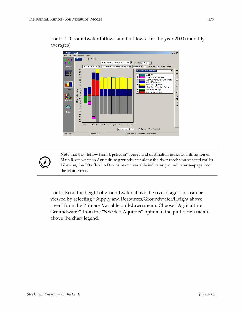
The Rainfall Runoff (Soil Moisture) Model 175
Look at “Groundwater Inflows and Outflows” for the year 2000 (monthly averages).
Note that the “Inflow from Upstream” source and destination indicates infiltration of Main River water to Agriculture groundwater along the river reach you selected earlier. Likewise, the “Outflow to Downstream” variable indicates groundwater seepage into the Main River.
Look also at the height of groundwater above the river stage. This can be viewed by selecting “Supply and Resources/Groundwater/Height above river” from the Primary Variable pull‐down menu. Choose “Agriculture Groundwater” from the “Selected Aquifers” option in the pull‐down menu above the chart legend.
Stockholm Environment Institute June 2005

176 WEAP Tutorial
Note that in the months where groundwater seepage to the Main River occurs (January to March), the groundwater elevation is higher than the wetted depth of the river designated in the data (i.e., the difference in elevations is positive). Likewise, when Main River infiltration to groundwater is occurring, the elevation difference is negative.
Stockholm Environment Institute June 2005