Water quality – Operative Evaluation of Small Streams’ Biological Quality by Saprobity Index of Macroinvertebrates Descriptors: water quality, saprobity index, benthic macroinvertebrates Foreword The Latvian Standard determines the method and procedure for the assessment of

long-term impact of pollution in small streams; the method is based on cenosis of

benthic macroinvertebrates. This method is applied for the assessment of biological

quality of small rivers and streams at full length or at stretches, as well as for the

determination of local impact of pollution.

According to this standard, only competent persons, or persons with higher education

in biology can do the analyses

The technical committee “Environmental quality” has worked out the Standard.

1. Introduction

An assessment of ecological quality based only on the chemical parameters is

incomplete because it reflects the ecological water quality only during the sampling.

The methods of biological analyses reflect water quality over a longer period of time.

In the assessment of water quality the cenoses of macroinvertebrates are more

important than those of plankton and they are more stable in time and space [1]. In the

states of European Union methods of biological analyses based on macroinvertebrates

are used for routine monitoring of rivers and the assessment of integrative water

quality, while they are less expensive and less time-consuming in comparison with

chemical analysis [2]. The results of analyses of water quality are represented on

coloured maps, therefore the information is easy available for none-specialists, as

each quality class has a corresponding colour and each stretch of river has been

coloured according to it’s water quality. The maps of water quality contain

information necessary for the boards of water resources, for frame of the regional

development planning and other decisions related with environmental protection and

conservation.

2. Scope

The method is used for assessment of long-term impact of organic pollution.

The method is used for the control of biological quality of small rivers and streams of

rithral and potamal type, with current velocity above 0,1 m/s. The method can be

applied for the investigation of the whole river or it’s single stretches, as well as for

the establishing of a local anthropogenic impact, for example, in the intake area of

wastewaters.

3. Definitions

Biotope – an area of waters or terrestrial part of land in which the main environmental

conditions as well as species composition are uniform;

Benthic macroinvertebrates – invertebrates living in sediments or on the bottom, or on

underwater objects; the size of organisms exceeds 1 mm;

Small rivers – rivers, the length of which does not exceed 100 km;

Potamal rivers – sandy and silty soft bottom slow running lowland rivers with current

velocity less than 0,2 – 0,3 m/s;

Rithral rivers – sandy and stony hard bottom fast flowing rivers with current velocity

above 0,2 – 0,3 m/s;

Saprobity – pollution of organic matter;

Saprobity index - numerical estimation of the pollution of organic matter, from 0 to 4.

Indicator organisms of saprobity – organisms, conformed for living at a specific level

of organic pollution.

Level of saprobity – a certain interval of organic pollution degree.

Zoocenosis – assemblage of organisms living in the biotope.

4. Principle

Sampling of indicator species of macroinvertebrates by using the bottom scraper.

Identification of organisms to the species or to other taxonomical levels. The

calculation of saprobity index.

5. Reagents

5.1. Ethyl alcohol, 70 %;

5.2. Formalin, 4 %;

6. Equipment and material

6.1. Bottom scraper; mesh size 0,5 or 1 mm;

6.2. Forceps;

6.3. Sorting tray (white);

6.4. Vials (10 ml) for transportation and storage of samples;

6.5. Thermooxymeter;

6.6. Turbidimeter;

6.7. Magnifying glass; amplification from 6 to 10 times;

6.8. Binocular;

7. The sampling and storage of samples A typical river stretch of 20 – 50 m is selected for sampling, where all the biotopes are investigated (by type of river-bed, composition of bottom, aquatic vegetation and current velocity) and their relative occurrence is determined. Occurrence of various biotopes in river stretches is given in Appendix D. The measuring of all the necessary parameters is done (water temperature, dissolved oxygen etc.). The physically – geographical state is described in the form “The protocol of testing the biological quality”. Explanatory notes on filling up the form are given in Appendix A. The macroinvertebrates are taken with a bottom scraper or picked with forceps from stones or branches or other underwater objects. At the selected reaches of rivers 20 individual samples of benthos are taken and tested like one median sample. The individual samples are taken according to the occurrence of all biotopes. For example, if 50 % of bottom consists of sand, 50 % of samples are taken from sandy biotopes. Organisms, picked from stones and branches, are considered as individual samples. Investigating the water quality at all length of the river, the frequency of sampling depends on homogeneity of environmental factors and biotopes. For example, in forested regions, with less anthropogenic impact, reaches for analyses are taken after each 5 km. If environmental (riverbank) conditions are changing or some signs of anthropogenic impact (canalised river, regulated flow, input of wastewater) are observed, the samples are taken in areas, where the environmental conditions are changing. If it is impossible to investigate the river at all it’s length, three sites of river are chosen – at the upper (headwaters), the middle and lower reaches. If it is necessary to establish the impact of point source pollution (input of wastewater’s), a 50 to 300 m long stretch of river (depending on current velocity and intensity of water mixing) is taken upstream and downstream from the pollution source.

The samples should be taken conversely to the current direction, in order to prevent

disturbance of confused bottom to biotopes downstream the sampling site.

An optimal season for sampling is the period of autumn – spring (from September

until July), because in summer macrozoobenthos is relatively poor.

8. Working design

The samples are put in a sorting tray and investigated at the stream to the relevant

taxonomical level, the number of individuals is counted and results are put in the

protocol of results (Appendix B). A magnifying glass and keys of identification are

used [6 – 10 or other]. If it is impossible to identify the organisms at the field, they

must be put in vials and fixed in ethyl alcohol (70%) or formalin (4%). The fixed

organisms should be kept in a dark place. Time of storage is unlimited.

At least 12 indicator organisms should be taken to obtain statistically significant

results, the sum of relative occurrence of organisms should be at least 30.

The saprobity index is calculated.

In case of necessity, non-fixed samples can be analysed at the laboratory.

9. Interpretation of results

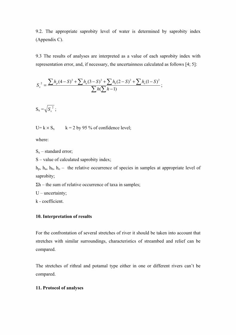
9.1. The calculation of saprobity index:

∑∑ ×

=i

ii

hhs

S ,

where: S - saprobity index;

si – individual saprobity index of i-th species [3];

hi - relative occurrence of i-th species in a sample.

9.2. The appropriate saprobity level of water is determined by saprobity index

(Appendix C).

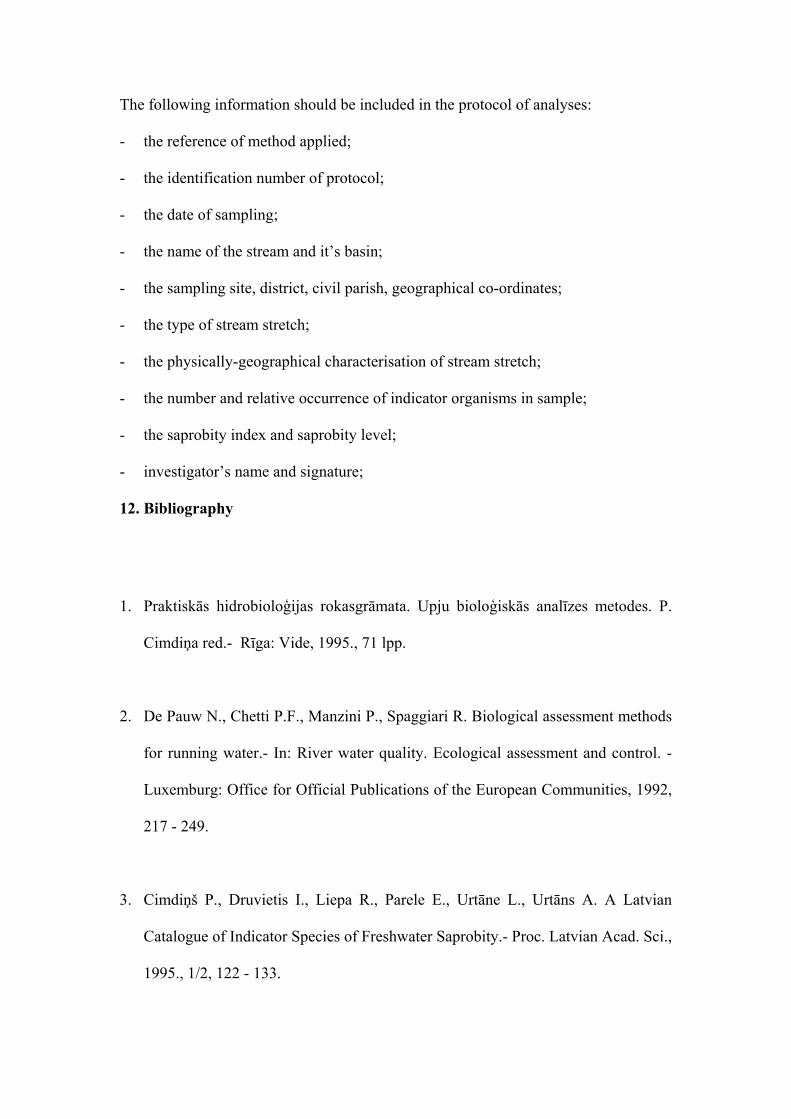
9.3 The results of analyses are interpreted as a value of each saprobity index with

representation error, and, if necessary, the uncertainness calculated as follows [4; 5]:

∑ ∑∑ ∑ ∑ ∑

−−+−+−+−

=)1(

)1()2()3()4( 22222

hhShShShSh

S obapx ;

Sx = 2xS ;

U= k × Sx k = 2 by 95 % of confidence level;

where:

Sx – standard error;

S – value of calculated saprobity index;

hp, ha, hb, ho – the relative occurrence of species in samples at appropriate level of

saprobity;

Σh – the sum of relative occurrence of taxa in samples;

U – uncertainty;

k - coefficient.

10. Interpretation of results

For the confrontation of several stretches of river it should be taken into account that

stretches with similar surroundings, characteristics of streambed and relief can be

compared.

The stretches of rithral and potamal type either in one or different rivers can’t be

compared.

11. Protocol of analyses

The following information should be included in the protocol of analyses:

- the reference of method applied;

- the identification number of protocol;

- the date of sampling;

- the name of the stream and it’s basin;

- the sampling site, district, civil parish, geographical co-ordinates;

- the type of stream stretch;

- the physically-geographical characterisation of stream stretch;

- the number and relative occurrence of indicator organisms in sample;

- the saprobity index and saprobity level;

- investigator’s name and signature;

12. Bibliography

1. Praktiskās hidrobioloģijas rokasgrāmata. Upju bioloģiskās analīzes metodes. P.

Cimdiņa red.- Rīga: Vide, 1995., 71 lpp.

2. De Pauw N., Chetti P.F., Manzini P., Spaggiari R. Biological assessment methods

for running water.- In: River water quality. Ecological assessment and control. -

Luxemburg: Office for Official Publications of the European Communities, 1992,

217 - 249.

3. Cimdiņš P., Druvietis I., Liepa R., Parele E., Urtāne L., Urtāns A. A Latvian

Catalogue of Indicator Species of Freshwater Saprobity.- Proc. Latvian Acad. Sci.,

1995., 1/2, 122 - 133.

4. Report of the ICES/HELCOM Workshop on Quality assurance of Benthic

Measurements in the Baltic Sea, Kiel, Germany, 23 – 25 March 1994.

5. Оценка степени загрязнения вод по организмам планктона и бентоса.

Методическое руководство. Красноярский гос. унив., 1982. 20 стр.

The keys of identification of benthic macroinvertebrates and other taxonomical

literature

6. Engelhardt W. Was lebt in Tümpel, Bach und Weicher? Stuttgart, 1989., 270 S.

7. Latvijas PSR dzīvnieku noteicējs. 1. daļa. Bezmugurkaulnieki (red. E. Tauriņš, E.

Ozols).Rīga: Latvijas Valsts izdevniecība, 1957., 871 lpp.

8. Lillehammer A. Stoneflies (Plecoptera) of Fennoscandia and Denmark.

Copenhagen: Scandinavian Science Press. 1988., 165 pp.

9. Определитель пресноводных беспозвоночных Европейской части СССР

(планктон, бентос).Ленинград: Гидрометеоиздат, 1977., 510 с.

10. Хейсин Е. М. Краткий определитель пресноводной фауны. Москва:

Государственное учебно-педагогическое издательство. 1962., 147 с.

APPENDIX A

(normative)

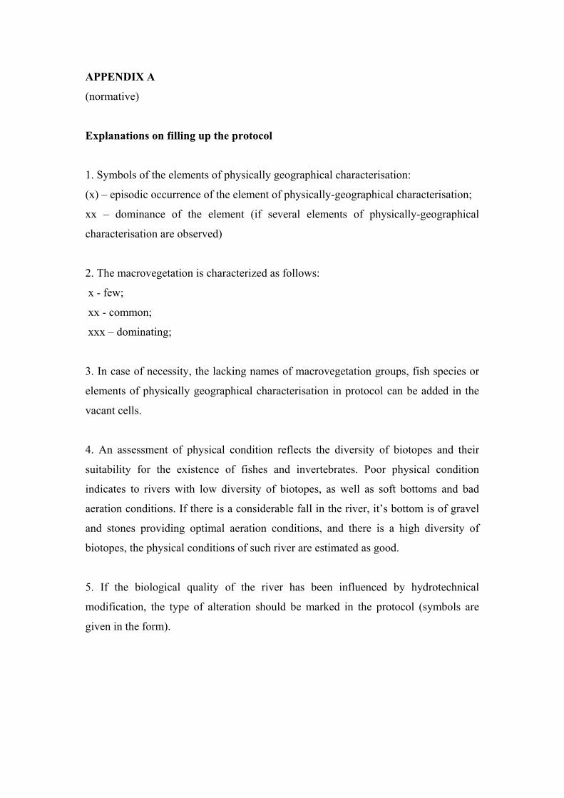
Explanations on filling up the protocol

1. Symbols of the elements of physically geographical characterisation:

(x) – episodic occurrence of the element of physically-geographical characterisation;

xx – dominance of the element (if several elements of physically-geographical

characterisation are observed)

2. The macrovegetation is characterized as follows:

x - few;

xx - common;

xxx – dominating;

3. In case of necessity, the lacking names of macrovegetation groups, fish species or

elements of physically geographical characterisation in protocol can be added in the

vacant cells.

4. An assessment of physical condition reflects the diversity of biotopes and their

suitability for the existence of fishes and invertebrates. Poor physical condition

indicates to rivers with low diversity of biotopes, as well as soft bottoms and bad

aeration conditions. If there is a considerable fall in the river, it’s bottom is of gravel

and stones providing optimal aeration conditions, and there is a high diversity of

biotopes, the physical conditions of such river are estimated as good.

5. If the biological quality of the river has been influenced by hydrotechnical

modification, the type of alteration should be marked in the protocol (symbols are

given in the form).

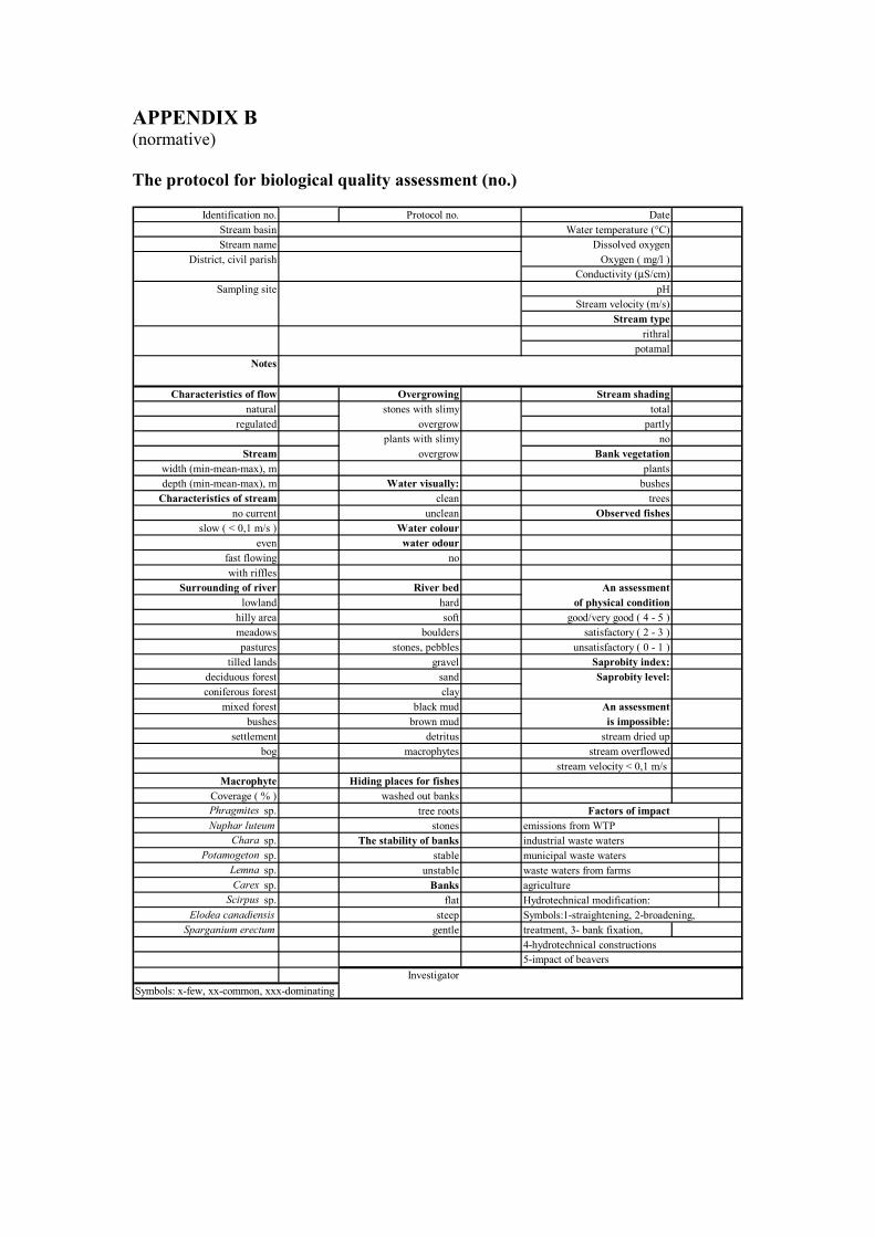
APPENDIX B (normative) The protocol for biological quality assessment (no.)

Identification no. Protocol no. DateStream basin Water temperature (°C)Stream name Dissolved oxygen

District, civil parish Oxygen ( mg/l ) Conductivity (µS/cm)

Sampling site pHStream velocity (m/s)

Stream type rithral

potamalNotes

Characteristics of flow Overgrowing Stream shadingnatural stones with slimy total

regulated overgrow partlyplants with slimy no

Stream overgrow Bank vegetationwidth (min-mean-max), m plantsdepth (min-mean-max), m Water visually: bushes

Characteristics of stream clean treesno current unclean Observed fishes

slow ( < 0,1 m/s ) Water coloureven water odour

fast flowing nowith riffles

Surrounding of river River bed An assessmentlowland hard of physical condition

hilly area soft good/very good ( 4 - 5 )meadows boulders satisfactory ( 2 - 3 )pastures stones, pebbles unsatisfactory ( 0 - 1 )

tilled lands gravel Saprobity index:deciduous forest sand Saprobity level:coniferous forest clay

mixed forest black mud An assessmentbushes brown mud is impossible:

settlement detritus stream dried upbog macrophytes stream overflowed

stream velocity < 0,1 m/s Macrophyte Hiding places for fishes

Coverage ( % ) washed out banks Phragmites sp. tree roots Factors of impact Nuphar luteum stones emissions from WTP

Chara sp. The stability of banks industrial waste waters Potamogeton sp. stable municipal waste waters

Lemna sp. unstable waste waters from farmsCarex sp. Banks agriculture

Scirpus sp. flat Hydrotechnical modification:Elodea canadiensis steep Symbols:1-straightening, 2-broadening,

Sparganium erectum gentle treatment, 3- bank fixation,4-hydrotechnical constructions5-impact of beavers

InvestigatorSymbols: x-few, xx-common, xxx-dominating

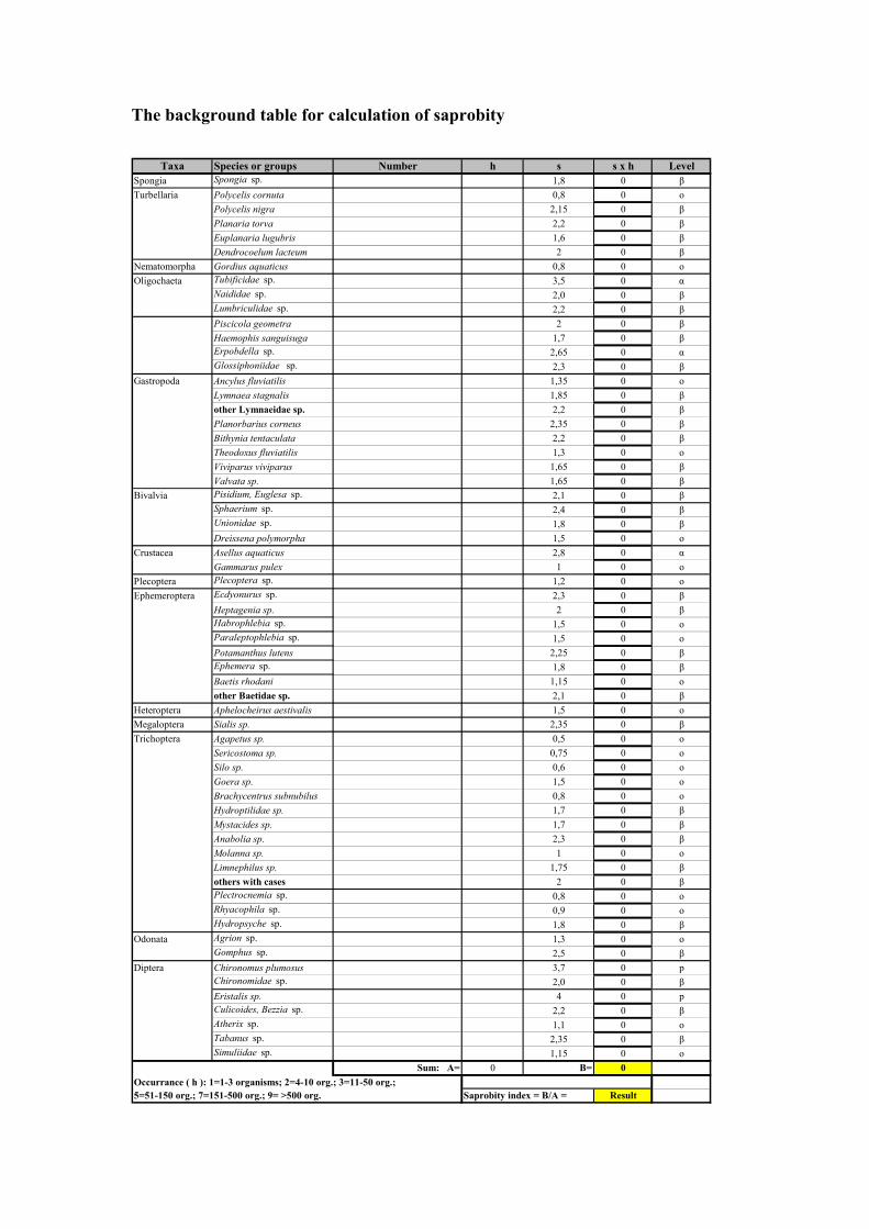
The background table for calculation of saprobity

Taxa Species or groups Number h s s x h LevelSpongia Spongia sp. 1,8 0 βTurbellaria Polycelis cornuta 0,8 0 o

Polycelis nigra 2,15 0 βPlanaria torva 2,2 0 βEuplanaria lugubris 1,6 0 βDendrocoelum lacteum 2 0 β

Nematomorpha Gordius aquaticus 0,8 0 oOligochaeta Tubificidae sp. 3,5 0 α

Naididae sp. 2,0 0 βLumbriculidae sp. 2,2 0 β

Piscicola geometra 2 0 βHaemophis sanguisuga 1,7 0 βErpobdella sp. 2,65 0 αGlossiphoniidae sp. 2,3 0 β

Gastropoda Ancylus fluviatilis 1,35 0 oLymnaea stagnalis 1,85 0 βother Lymnaeidae sp. 2,2 0 βPlanorbarius corneus 2,35 0 βBithynia tentaculata 2,2 0 βTheodoxus fluviatilis 1,3 0 oViviparus viviparus 1,65 0 βValvata sp. 1,65 0 β

Bivalvia Pisidium, Euglesa sp. 2,1 0 βSphaerium sp. 2,4 0 βUnionidae sp. 1,8 0 βDreissena polymorpha 1,5 0 o

Crustacea Asellus aquaticus 2,8 0 αGammarus pulex 1 0 o

Plecoptera Plecoptera sp. 1,2 0 oEphemeroptera Ecdyonurus sp. 2,3 0 β

Heptagenia sp. 2 0 βHabrophlebia sp. 1,5 0 oParaleptophlebia sp. 1,5 0 oPotamanthus lutens 2,25 0 βEphemera sp. 1,8 0 βBaetis rhodani 1,15 0 oother Baetidae sp. 2,1 0 β

Heteroptera Aphelocheirus aestivalis 1,5 0 oMegaloptera Sialis sp. 2,35 0 βTrichoptera Agapetus sp. 0,5 0 o

Sericostoma sp. 0,75 0 oSilo sp. 0,6 0 oGoera sp. 1,5 0 oBrachycentrus subnubilus 0,8 0 oHydroptilidae sp. 1,7 0 βMystacides sp. 1,7 0 βAnabolia sp. 2,3 0 βMolanna sp. 1 0 oLimnephilus sp. 1,75 0 βothers with cases 2 0 βPlectrocnemia sp. 0,8 0 oRhyacophila sp. 0,9 0 oHydropsyche sp. 1,8 0 β

Odonata Agrion sp. 1,3 0 oGomphus sp. 2,5 0 β

Diptera Chironomus plumosus 3,7 0 pChironomidae sp. 2,0 0 βEristalis sp. 4 0 pCulicoides, Bezzia sp. 2,2 0 βAtherix sp. 1,1 0 oTabanus sp. 2,35 0 βSimuliidae sp. 1,15 0 o

Sum: A= 0 B= 0Occurrance ( h ): 1=1-3 organisms; 2=4-10 org.; 3=11-50 org.;5=51-150 org.; 7=151-500 org.; 9= >500 org. Saprobity index = B/A = Result

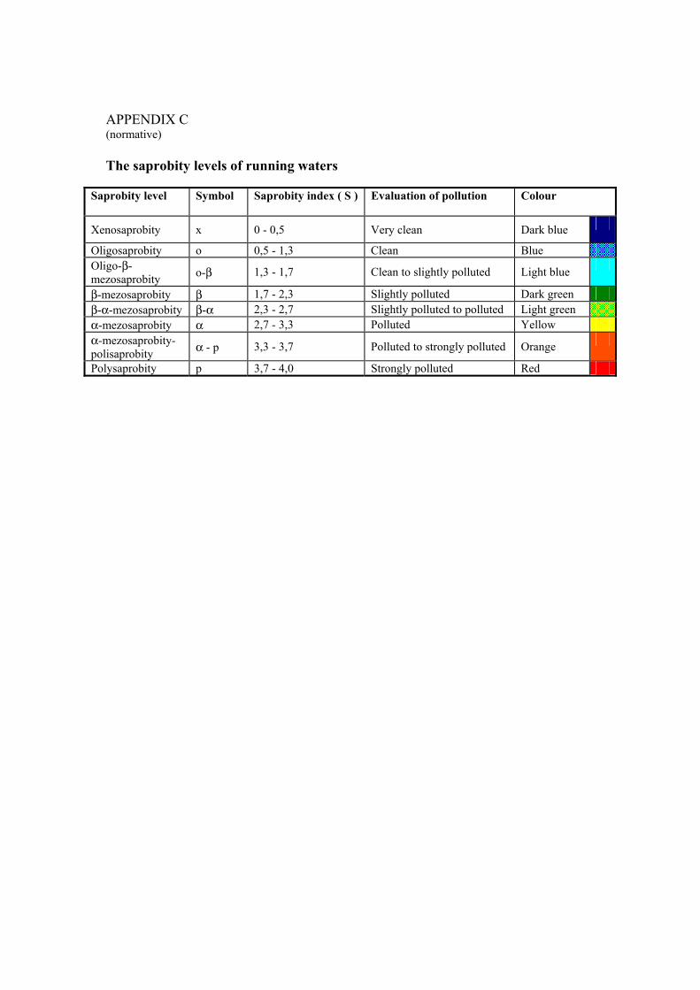
APPENDIX C (normative) The saprobity levels of running waters

Saprobity level

Symbol Saprobity index ( S ) Evaluation of pollution Colour

Xenosaprobity x 0 - 0,5 Very clean Dark blue

Oligosaprobity o 0,5 - 1,3 Clean Blue Oligo-β-mezosaprobity o-β 1,3 - 1,7 Clean to slightly polluted Light blue

β-mezosaprobity β 1,7 - 2,3 Slightly polluted Dark green β-α-mezosaprobity β-α 2,3 - 2,7 Slightly polluted to polluted Light green α-mezosaprobity α 2,7 - 3,3 Polluted Yellow α-mezosaprobity- polisaprobity α - p 3,3 - 3,7 Polluted to strongly polluted Orange

Polysaprobity p 3,7 - 4,0 Strongly polluted Red

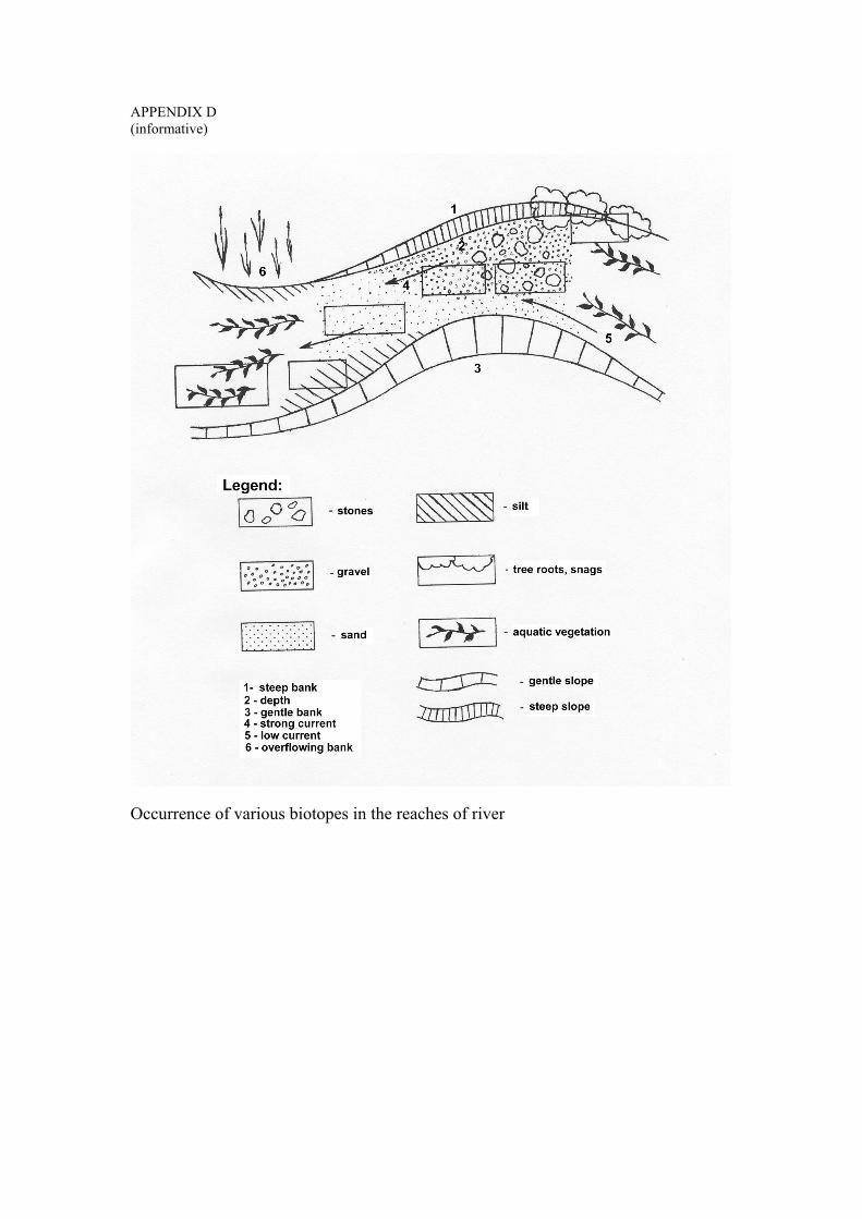
APPENDIX D (informative)

Occurrence of various biotopes in the reaches of river