water quality statistical and˜ pollutant loadinsg …...table 5-6. kendall’s tau correlation...

Green-Duwamish WatershedWater Quality Assessment

October 2006

WATER QUALITY STATISTICAL AND�POLLUTANT LOADINSG ANALYSIS

Prepared for

Department of Natural Resources and Parks��

��

��

�� !��"��

#��"�$%%&

Note: Some blank pages in this document have been purposefully skipped for improved online viewing.

WATER QUALITY STATISTICAL AND

POLLUTANT LOADINGS ANALYSIS

Green-Duwamish Watershed

Water Quality Assessment

Prepared for

Prepared by

Herrera Environmental Consultants, Inc. 2200 Sixth Avenue, Suite 1100

Seattle, WA 98121 Telephone: 206/441-9080

In association with

Anchor Environmental, L.L.C. and Northwest Hydraulic Consultants, Inc.

January 19, 2007

i

Contents

Executive Summary ...................................................................................................................... vii

1.0 Introduction........................................................................................................................... 1-1

1.1 Purpose and Objectives of Monitoring Program and Analysis ..................................... 1-2 1.2 Report Organization ...................................................................................................... 1-7

2.0 Overview of Green-Duwamish Watershed........................................................................... 2-1

2.1 Green-Duwamish Watershed......................................................................................... 2-1 2.2 Major Stream Basins and Tributary Subbasins ............................................................. 2-2

2.2.1 Springbrook Creek Basin.............................................................................. 2-2 2.2.2 Mill (Hill) Creek Basin................................................................................. 2-2 2.2.3 Soos Creek Basin.......................................................................................... 2-7 2.2.4 Newaukum Creek Basin ............................................................................... 2-7 2.2.5 Hamm Creek Subbasin ................................................................................. 2-7 2.2.6 Lea Hill Subbasin ......................................................................................... 2-7 2.2.7 Crisp Creek Subbasin ................................................................................... 2-8

3.0 Overview of Monitoring for the Green-Duwamish Water Quality Assessment .................. 3-1

3.1 Site Locations ................................................................................................................ 3-1 3.2 Sample Types and Sampling Frequency ....................................................................... 3-8

3.2.1 Base Flow Samples....................................................................................... 3-8 3.2.2 Storm Flow Samples..................................................................................... 3-9

3.3 Sample Collection Procedures....................................................................................... 3-9 3.3.1 Manual Grab Samples................................................................................... 3-9 3.3.2 Auto-Sequential Samples............................................................................ 3-10 3.3.3 Auto-Composite Samples ........................................................................... 3-10 3.3.4 Instream Field Measurements..................................................................... 3-11

3.4 Sample Documentation and Handling Procedures ...................................................... 3-11 3.4.1 Sample Documentation............................................................................... 3-11 3.4.2 Sample Handling ........................................................................................ 3-12

3.5 Analytical Parameters.................................................................................................. 3-12 3.6 Laboratory Analysis Methods ..................................................................................... 3-13

3.6.1 Conventional Parameters ............................................................................ 3-13 3.6.2 Nutrients ..................................................................................................... 3-13 3.6.3 Indicator Bacteria........................................................................................ 3-14 3.6.4 Metal and Mineral Analyses....................................................................... 3-14 3.6.5 Organic Analyses and Detection Limits ..................................................... 3-14

3.7 Quality Control Procedures ......................................................................................... 3-14 3.8 Data Reporting Procedures.......................................................................................... 3-15 3.9 Data Management Procedures..................................................................................... 3-16

4.0 Data Analysis Methods......................................................................................................... 4-1

ii

4.1 Water Quality Statistical Analysis................................................................................. 4-1 4.1.1 Comparison of Routine and GDWQA Sampling Approaches ..................... 4-1 4.1.2 Comparison of Storm and Base Flow Concentrations.................................. 4-2 4.1.3 Comparison of Rising and Falling Limbs of Storm Hydrograph ................. 4-2 4.1.4 Correlation among Water Quality Parameters.............................................. 4-5 4.1.5 Correlation between Water Quality and Hydrologic Parameters ................. 4-6 4.1.6 Principal Component Analysis ..................................................................... 4-6

4.2 Pollutant Loadings and Land Use Analyses.................................................................. 4-7 4.2.1 Loading Calculations .................................................................................... 4-7 4.2.2 Loading – Land Use/Cover Analysis.......................................................... 4-12

5.0 Results................................................................................................................................... 5-1

5.1 Water Quality Statistical Analysis................................................................................. 5-1 5.1.1 Comparison of Routine and GDWQA Sampling Approaches ..................... 5-1 5.1.2 Comparison of Parameters in Storm Flow and Base Flow........................... 5-3 5.1.3 Comparison of Rising and Falling Limbs of Storm Hydrograph ................. 5-5 5.1.4 Correlations among Water Quality Parameters ............................................ 5-6 5.1.5 Correlation between Water Quality and Hydrologic Parameters ............... 5-10 5.1.6 Principal Component Analysis ................................................................... 5-15

5.2 Pollutant Loading Analysis ......................................................................................... 5-16 5.2.1 Loading Rate Analysis................................................................................ 5-16 5.2.2 Land Use Loading Analysis........................................................................ 5-17 5.2.3 Comparison of Land Use Loading Factors to Literature Values................ 5-28 5.2.4 Land Use Loading Correlation ................................................................... 5-37

6.0 Conclusions........................................................................................................................... 6-1

6.1 Agricultural Land .......................................................................................................... 6-1 6.2 Forested Land ................................................................................................................ 6-2 6.3 Developed Areas ........................................................................................................... 6-2

7.0 Implications of Study Results............................................................................................... 7-1

7.1 Implications for Monitoring .......................................................................................... 7-1 7.1.1 Monitoring Site Locations ............................................................................ 7-1 7.1.2 Sampling Method.......................................................................................... 7-1 7.1.3 Constituent Testing....................................................................................... 7-2

7.2 Implications for Modeling............................................................................................. 7-2 7.3 Implications for Management........................................................................................ 7-3

7.3.1 Management of Riparian Areas .................................................................... 7-3

8.0 References............................................................................................................................. 8-1

Appendix A Comparison of Water Quality Results from Different Sampling Protocols for King

County’s Ambient and Green-Duwamish Watershed Water Quality Assessment monitoring programs, 2001 through 2003

iii

Appendix B Comparison of Water Quality Data Collected during Storm Flow and Base Flow Conditions in the Green-Duwamish Watershed, 2001 through 2003

Appendix C Alkalinity and Total Suspended Solids Hysteresis Loops from Select Sites within the Green-Duwamish Watershed, 2001 through 2003

Appendix D Water Quality Constituent Correlation Tables, Green-Duwamish Watershed, 2001 through 2003

Tables

Table 3-1. Basin area, impervious area, and land cover characteristics by monitoring site for the Green-Duwamish watershed water quality assessment. ....................... 3-5

Table 3-2. Impervious area and land cover characteristics by monitoring site for the Green-Duwamish watershed water quality assessment as assessed for a 200 meter buffer surrounding the major waterways in each basin.. .............................. 3-6

Table 3-3. Impervious area and land cover characteristics by monitoring site for the Green-Duwamish watershed water quality assessment as assessed for a 200 by 1000 meter upstream polygon for each sample site........................................... 3-7

Table 3-4. Sampling dates for the Green-Duwamish watershed water quality assessment............................................................................................................... 3-8

Table 4-1. Number of data points (base flow/storm flow) by parameter evaluated for each monitoring site in the Green-Duwamish watershed water quality assessment (2001 through 2003)............................................................................. 4-3

Table 4-2. Tributary sites used for land use loading analysis. ............................................... 4-12

Table 4-3. Description of GIS data sources and quality control edits.................................... 4-14

Table 4-4. Final land use/cover categories for the Green-Duwamish watershed................... 4-15

Table 5-1. Percentage of constituents for which the highest median and maximum values were observed among the four GDWQA sampling approaches.................. 5-2

Table 5-2. Ratio of median storm to base flow concentrations for sites in the Green-Duwamish watershed, 2001 – 2003. ....................................................................... 5-4

Table 5-3. Summary of hysteresis analysis for alkalinity and total suspended solids, categorizing slope and direction of hysteresis for each of the 24 storms analyzed. ................................................................................................................. 5-7

Table 5-4. Correlations observed among the various water quality parameters monitored in the GDWQA...................................................................................... 5-8

Table 5-5. Kendall’s Tau correlation matrix of water quality parameters versus flow statistics for the five storms monitored in predominantly agricultural basins. ..... 5-11

iv

Table 5-6. Kendall’s Tau correlation matrix of water quality parameters versus flow statistics for the six storms monitored in predominantly forested basins. ............ 5-12

Table 5-7. Kendall’s Tau correlation matrix of water quality parameters versus flow statistics for the 11 storms monitored in basins with predominantly low-density residential development............................................................................ 5-14

Table 5-8. Kendall’s Tau correlation matrix of water quality parameters versus flow statistics for the 10 storms monitored in predominantly highly developed basins..................................................................................................................... 5-15

Table 5-9. Pollutant loading values for base flow, runoff, and total annual loads in 13 subbasins of the Green-Duwamish watershed (2001 through 2003). ................... 5-21

Table 5-10. Ratio of annual pollutant runoff loading to base flow loading in 13 subbasins of the Green-Duwamish watershed (2001 through 2003). ................... 5-25

Table 5-11. Areal pollutant loading values for base flow, runoff, and total annual loads in 13 subbasins of the Green-Duwamish watershed (2001 through 2003). .......... 5-29

Table 5-12. Areal pollutant loading values for base flow, runoff, and total annual loads in tributary subbasins representative of land use/cover categories in the Green-Duwamish watershed (2001 through 2003)............................................... 5-33

Table 5-13. Comparison of areal loading rates calculated from the Green-Duwamish watershed assessment to areal loading rates from the literature and previous King County studies.............................................................................................. 5-35

Table 5-14. Kendall’s Tau correlations between total watershed land use/cover and annual constituent loading in the major streams and tributaries of the Green-Duwamish watershed. ........................................................................................... 5-39

Table 5-15. Kendall’s Tau correlations among land use/cover categories in the Green-Duwamish watershed. ........................................................................................... 5-43

Table 5-16. Kendall’s Tau correlations between 200-meter buffer land use/cover and annual constituent loading in the major streams and tributaries of the Green-Duwamish watershed. ........................................................................................... 5-45

v

Figures

Figure 1-1. Location of Green-Duwamish watershed in King County, Washington. ............ 1-3

Figure 1-2. Monitoring sites in the Green-Duwamish watershed........................................... 1-5

Figure 2-1. Monitoring sites and land uses/covers in the Green-Duwamish watershed. ....... 2-3

Figure 2-2. Schematic diagram of monitoring sites for the Green-Duwamish watershed water quality assessment..................................................................... 2-5

Figure 3-1. Areal percentage of land use/cover categories in 17 subbasins in the Green-Duwamish watershed................................................................................ 3-3

Figure 4-1. Example hydrograph from Soos Creek (A320) showing delineation of base and storm flow events in 2003..................................................................... 4-9

Figure 4-2. Flow chart depicting the calculation of annual flow-weighted mean concentrations in the Green-Duwamish watershed water quality assessment, 2001 through 2003. ........................................................................ 4-11

Figure 4-3. Flow chart depicting the calculation of annual loadings in the Green-Duwamish watershed water quality assessment, 2001 through 2003................ 4-11

Figure 5-1. A 15-day hydrograph separation derived from analysis of silicon dioxide (SiO2) and oxygen-18 (18O) isotope relationships between different water sources.................................................................................................................. 5-6

Figure 5-2. Projection of the variables on the factor plane................................................... 5-18

Figure 5-3. Projection of data (grouped by watershed land use) on the factor plane ........... 5-19

Water Quality Analysis—Green-Duwamish Watershed

lmp /02-01039-000 green-duwamish loading report.doc

January 19, 2007 vii King County Department of Natural Resources and Parks

Executive Summary

The primary goal of the Green-Duwamish Watershed Water Quality Assessment (GDWQA) is to provide analytical tools to evaluate current and potential water quality issues in the Green – Duwamish River watershed. This report assesses and analyzes the water quality data collected for the GDWQA during water years 2002 and 2003. Analyses performed on the data include:

Comparison of the ambient and GDWQA sampling approaches Comparison of water quality data for base flow and storm flow Hysteresis analysis for total suspended solids and alkalinity Correlation analysis among water quality parameters Correlation analysis between water quality and hydrologic parameters Principal component analysis Pollutant loading rate analysis Correlation analysis between pollutant loadings and land use/cover

categories.

Sampling Approach Comparison

A comparison of the ambient (routine) monitoring program (which uses a grab sampling approach conducted monthly plus six storms per year ) and the GDWQA monitoring program (which used grab, automated sequential, and automated composite sampling approaches) indicated that the sequential sampling approach was the most effective at capturing maximum concentrations during storms. However, the ambient monitoring program was also effective and could be used as a surrogate for sequential sampling when such sampling is not possible due to field sampling personnel, equipment, or sample analysis budget constraints. It was difficult to compare the GDWQA grab sampling approach and the ambient grab sampling program because of low number of grab samples collected for the GDWQA. Both of the grab sampling programs had the highest percentage of constituents with maximum median values for base and storm flow. Assuming that composite sampling with automated equipment provides the most accurate estimate of the median concentration, the data suggest that there is a slight upward bias in determining median pollutant concentrations from grab sampling programs. Consequently, if an event mean concentration (EMC) approach is used to calculate pollutant loadings, a grab sampling approach would likely overestimate those loadings. However, if a regression approach is used to estimate pollutant loadings, a grab sampling approach could provide acceptable and defensible results because concentrations are flow weighted with the regression approach.

Storm and Base Flow Comparison

By comparing storm flow to base flow constituent concentrations, useful information can be garnered regarding the processes driving water quality in the watershed. Storm/base flow



King County viii January 19, 2007 Department of Natural Resources and Parks

concentration ratios indicated that agricultural sites had highly elevated storm flow concentrations of indicator bacteria and phosphorus. Metals concentrations were consistently higher in storm flow than in base flow, indicating the importance of storms in metals loading and transport. Dissolved oxygen (DO) and pH were generally not significantly different when comparing base flow and storm flow across the 17 analyzed sites, except at one site, Springbrook Creek (A317) where DO increased during storm flow from depressed base flow DO levels. The findings from this analysis were supported in many of the other analyses, indicating that storm/base flow concentration ratios are a simple and useful analysis tool.

Hysteresis Analysis

A hysteresis analysis of total suspended solids (TSS) concentrations and alkalinity values during individual storm events indicated that a TSS (sediment) first flush effect exists for the majority (54 percent) of storms analyzed, and an alkalinity first flush exists for approximately 25 percent of the analyzed storms. All of the total suspended solids hysteresis loops had a positive slope, while nearly all of the alkalinity hysteresis loops had negative slopes. These slopes indicate that, with increasing discharge during the rising limb of the hydrograph, TSS increases while alkalinity decreases. The one agricultural site used in this analysis (site D322 dominated by livestock pastureland) exhibited the most consistent sediment and alkalinity first-flush pattern, a possible indication of riparian erosion from grazing practices and high bicarbonate concentration in stormwater runoff (and interflow) during the rising limb of the hydrograph. Newaukum Creek (site 0322) and the forested tributary (site S322) used in the analysis also exhibited an alkalinity first-flush pattern, suggesting that bicarbonates are flushed from soils during the rising limb of the hydrograph in forested and agricultural basins. The only sites exhibiting a counterclockwise alkalinity hysteresis were located in developed basins. This implies that runoff (and interflow) from developed basins is ionically dilute, a factor that can be explained by the fact that storm flow in these basins is largely routed over impervious surfaces, thereby having minimal contact with solute-rich soils.

Correlation among Water Quality Parameters

A correlation analysis among water quality parameters is useful for grouping parameters into “families” which behave the same in surface waters. The data indicate that total phosphorus, total suspended solids, turbidity, fecal coliform bacteria, E. coli, and all metals (except dissolved iron) are frequently correlated. All of these constituents are elevated during storm flow, which explains why the correlation exists. The other major pattern in the water quality correlation data is that alkalinity, hardness, and specific conductance (which are all measures of dissolved substances) tend to be negatively correlated with those constituents which are exported during storms. These patterns are due to the fact that during storm events, dilute rainfall washes particulate-borne pollutants into receiving waters, while simultaneously diluting solute-rich base flow.



January 19, 2007 ix King County Department of Natural Resources and Parks

Correlation of Water Quality Parameters to Hydrologic Parameters

A correlation analysis of water quality parameters to hydrologic parameters led to many of the same conclusions noted above. In agricultural basins there was a strong negative (significant) correlation between nitrate+nitrite nitrogen and average event flow, indicating that maximum nitrate+nitrite nitrogen concentrations occurred during base flow and small storms, when dissolved nitrogen was flushed from soils but not diluted by a large quantity of rainwater. In addition, most constituents (expect TSS, turbidity, and pH) showed a weak negative (not significant) correlation with total event flow, peak event flow, average event flow, and standard deviation of event flow. These correlations indicate that rainwater dilution during large storms was a controlling factor for stream hydrochemistry.

Unlike the agricultural catchments, there was no synoptic pattern of negative correlation between water quality parameters and flow statistics in the forested basins studied. This lack of correlation may indicate that differences in the chemistry between rainwater and deep and shallow groundwater are less pronounced in forested catchments relative to agricultural basins. In highly-developed basins, dissolved and total copper and zinc were positively correlated with the antecedent dry period. These correlations indicate that these metals accumulate during dry weather and then wash off at high concentrations during subsequent storms. This analysis provides evidence that first-flush dynamics are applicable for these metals in urban watersheds.

Principal Component Analysis

A principal component analysis was used to group water quality variables and to relate those groups to land use patterns. The first principal component explained 45.5 percent of the total variance in the observed concentrations of water quality constituents. This component was primarily controlled by constituents that increase or are modified in urban and agricultural areas (e.g., metals, total suspended solids, nitrogen, phosphorus, pH and DO). All measured constituents (except for specific conductance, hardness, and alkalinity) clustered around this axis. When the variables were grouped by land use/cover category, the component 1 axis appeared to represent a gradient of development from forest on the right side of the axis towards urban and agriculture on the left. Therefore, it can be inferred that the variability in water quality between these land use/cover categories explains 45.5 percent of the variation in the data set.

The second principal component explained 16.1 percent of the variance in the data and was strongly controlled by specific conductance, hardness, and alkalinity. These dissolved constituents are higher in groundwater than stormwater (except in some agricultural basins); therefore, the second principal component might be interpreted as a base flow versus storm flow component. This analysis was useful in that it provided a simple reduction of the data that aided the characterization of broad patterns across the data structure.



King County x January 19, 2007 Department of Natural Resources and Parks

Pollutant Loading Rate Analysis

Pollutant loading rate analysis indicated that for the majority of water quality constituents, the pollutant mass exported during runoff events was greater than the mass exported during base flow. However, a few constituents, including dissolved nutrients (e.g., orthophosphate phosphorus) and dissolved iron, were exported primarily during base flow. For the majority of sites, base flow volumes were higher than runoff volumes. The routing of winter base flow to storm flow was evident in developed basins because only the developed areas exported more water during runoff events than during base flow events. During base flow, forested sites had lower areal loading rates for metals compared to developed sites, but forested sites had higher loading rates for nutrients and total suspended solids compared to developed sites due to the higher areal hydraulic loading rates for forested sites during base flow.

Runoff areal loading rates for total suspended solids, indicator bacteria, and metals were substantially greater in developed areas than in undeveloped areas. Although areal hydraulic loading rates were greater in developed areas than in agricultural areas, runoff areal loading rates of nutrients were greatest from agricultural lands, where source areas tend to be larger and more concentrated than those in urban areas.

A comparison of GDWQA loading rates with previous King County loading rates and literature loading rates from across the nation indicated that loading rates in the previous King County studies and Green-Duwamish data sets were generally higher than those in the literature. Variability between the King County and Green-Duwamish loading data was greatest for the agricultural land use/cover category. This may be explained by the fact that only one agricultural site was used in this areal loading analysis. If additional sites had been used, a more representative areal loading rate may have been obtained. Despite this difference, the Green-Duwamish data set reports loadings for a number of constituents that are not included in the previous King County data set. These additional loading values can be used to improve the overall accuracy of predicting water quality impacts from different types of land use.

It should be noted that these land use loading rates were derived from averaging loading rates across basins categorized by the dominant land use within the basin. Consequently, there can be considerable variability across the categorized basins that are not reflected in the final land use loading value. For example, at site A307 (Hamm Creek, a low- to medium-density development site), the total suspended solids areal loading rate (381.5 kg/ha/yr) was the highest observed in the entire study area. Conversely, the lowest total suspended solids areal loading rate (40.4 kg/ha/yr) was observed at site Y320 (Soosette Creek), which is another low- to medium-density development basin. This indicates that variability among low- to medium-density development sites can be very high and that broad land use categorization should be used with caution.



January 19, 2007 xi King County Department of Natural Resources and Parks

Correlation of Pollutant Loadings to Land Use

Correlations between total annual constituent loadings and land use/cover categories showed that those land use characteristics most consistently associated with increased pollutant loading include commercial/industrial, high-density residential, agriculture, and effective impervious area. Conversely, forest and low-density residential were the land use/cover categories most consistently negatively correlated with pollutant loading. Commercial/industrial land use exhibited significant positive correlations with ammonia nitrogen, total zinc, and dissolved iron. The high-density residential land use/cover category exhibited positive and significant correlations with fecal coliform bacteria and dissolved zinc. Agriculture was most strongly correlated with orthophosphate phosphorus, total phosphorus, and dissolved copper. Effective impervious area showed significant positive correlations with E. coli, ammonia nitrogen, total copper, total mercury, and total and dissolved zinc.

Also of interest was a positive correlation between the percentage of roads (areal coverage) within a basin and dissolved zinc. When base flow loading was used instead of total annual loading in the correlation analysis, low-density residential land use became negatively correlated with numerous constituents: total suspended sediment, nitrate+nitrite nitrogen, orthophosphate phosphorus, total phosphorus, dissolved and total copper, total mercury, and dissolved and total iron. This finding suggests that low-density residential development does not seriously impact pollutant loading, especially during base flow conditions.

The land use loading correlation analysis was conducted separately for land use in the entire subbasin draining to the tributary/stream site and for land use in a 200-meter buffer area adjacent to the entire length of the tributary/stream. The results of these analyses indicated that, after limiting the land use categories used in the analysis to a 200-meter buffer, the correlation between some land use categories and pollutant loading increased, whereas other relationships became insignificant. There was not, however, a clear pattern as to which relationships weakened and which grew stronger. Consequently, the use of both methods (200-meter buffer and whole watershed land use) should be considered in any future pollutant loading analyses.



January 19, 2007 1-1 King County Department of Natural Resources and Parks

1.0 Introduction

Since 1970, King County (and previously the Municipality of Metropolitan Seattle) has conducted water quality sampling in the Green-Duwamish watershed, which is located in southern King County, Washington (Figure 1-1). In the past, the goal of this monitoring has been to provide information about local surface waters in the Seattle/King County metropolitan area in support of programs designed to protect water quality and abate water pollution. In 2001, King County initiated a focused comprehensive study of the Green-Duwamish watershed, called the Green-Duwamish Watershed Water Quality Assessment (GDWQA) Comprehensive Monitoring Program. The primary goal of this program is to collect and analyze water quality data within the Green-Duwamish watershed and to use these data to support the following efforts and teams (King County 2002):

Wastewater Treatment Division Habitat Conservation Plan team

The Water Treatment Division combined sewer overflow control planning team

The Water Resource Inventory Area (WRIA) 9 Planning Work Group, Technical Committee and Steering Committee

Washington State Department of Ecology total maximum daily load efforts

King County Freshwater Monitoring Program.

The primary objectives of this monitoring program are to develop analytical tools for evaluating current and future water quality and quantity issues in the Green-Duwamish watershed, to coordinate with the WRIA 8 and 9 Steering Committee/Planning Groups as well as the Sammamish-Washington Assessment and Modeling Program (SWAMP) Team, and to provide water quality information to clients, both internal and external to the King County Department of Natural Resources and Parks. For example, data from the GDWQA will be used for wastewater capital planning, WRIA 9 salmon conservation planning, stormwater management efforts, and the Washington State Department of Ecology total maximum daily load program.

In support of this monitoring program, Herrera Environmental Consultants, Inc. (Herrera) was retained by King County to evaluate and summarize water quality data collected for the Green-Duwamish watershed from 2001 through 2003 (Herrera 2004, 2005). Since these data reports were prepared, detailed analyses of the 2001–2003 data have been performed, including statistical analysis to explore relationships between hydrologic and water quality parameters. Pollutant loading factors have also been calculated and analyzed for specific land uses within the Green-Duwamish watershed. This report describes the methods used for these analyses, presents the results of the analyses, and presents the major conclusions from these analyses. The ultimate goal of the analyses presented herein is to provide a framework for understanding how changes



King County 1-2 January 19, 2007 Department of Natural Resources and Parks

in land use/cover within the watershed is manifested in the water quality record. The results from this study will be used to improve calibration of current King County water quality models and serve as a guide for future monitoring efforts.

1.1 Purpose and Objectives of Monitoring Program and Analysis

The objectives of the GDWQA Comprehensive Monitoring Program are as follows:

Measure water quality parameters in different geographic areas of the watershed throughout the year, including at the mouths of major tributaries and at subwatershed boundaries within the main stem Green River.

Measure water quality parameters resulting from different land use/cover categories within select tributary subbasins.

Measure water quality parameters in the main stem, major streams, and select tributaries during both storm flow and base flow conditions.

Measure water quality parameters as a function of the rise, peak, and fall of the corresponding stream hydrograph to determine the variability of parameters during a storm.

Collect sufficient data to support development and calibration of water quality models for the Green-Duwamish watershed

Collect water quality data that can be used regionally.

Water quality monitoring for the GDWQA was conducted according to the sampling and analysis plan previously developed by King County (2002). The monitoring involved the collection of water samples at 18 sites located in the lower and middle segments of the Green-Duwamish watershed. Two of these sites are located on the main stem of the Green River, and five sites are located near the mouths of four major tributary streams: Springbrook Creek (Black River), Mill Creek, Soos Creek, and Newaukum Creek. The other 11 sites are located on tributaries representing different land uses, including forest (three sites), agriculture (two sites), low- to medium-density development (four sites), and high-density development (two sites) (King County 2002). Due to limited, insufficient sampling at an upland forested tributary (Green River Tributary near TPU, A341), only 17 sites were used for the majority of the analyses. These 17 sites are shown in Figure 1-2. Additionally, data from only 13 sites were used in the loading analysis due to incomplete flow records and/or infrequent monitoring (see section 4.2).

King County

Snohomish County

Pierce County

KittitasCounty

KitsapCounty

Seattle

JeffersonCounty

Green-Duwamish Watershed Study Area

WASHINGTON

OREGON

IDAH

O

Area of map detail

Pacif

ic Oc

ean

CANADA

Figure 1-1. Location of Green-Duwamish watershed study area in King County, Washington.Prepared for King County by Herrera Environmental ConsultantsKing County




This report presents results from detailed analyses of monitoring data collected for the GDWQA and the King County Stream and River Ambient Monitoring Program over a two year period between November 2001 and October 2003. The specific objectives of this analysis were as follows:

Evaluate differences between pollutant concentrations in storm flow and base flow.

Evaluate differences between water quality data collected through the GDWQA and King County’s ongoing Stream and River Ambient Monitoring Program.

Evaluate potential relationships between pollutant concentrations and storm size, storm intensity, and antecedent conditions.

Analyze storm flushing dynamics as they relate to land use.

Calculate pollutant loadings for monitored base flow and storm flow events, and estimate annual loadings of selected pollutants of concern for all monitoring sites.

Develop annual pollutant loading rates and land use pollutant loading rates for each land use/cover category based on relationships observed between measured concentrations, discharge, and land use in the monitored basins, and compare these rates to those used for watershed modeling and published in the literature.

Evaluate the potential effects of actual land use/cover upstream of the associated monitoring site on pollutant loading rates for each monitored basin.

1.2 Report Organization

The remainder of this report is organized into the following sections:

Section 2.0 (Overview of Green-Duwamish Watershed): Describes the physical features and land use characteristics of the Green-Duwamish River and its tributaries.

Section 3.0 (Overview of Monitoring for Green-Duwamish Water Quality Assessment): Summarizes sampling locations, sample types and sampling frequency, sample collection procedures, sample documentation and handling procedures, sampling parameters, laboratory analysis methods,




quality control procedures, and data reporting and recordkeeping procedures.

Section 4.0 (Data Analysis Methods): Describes the procedures used for data compilation and management, as well as the specific data analysis methods that were used to meet the objectives of this analysis.

Section 5.0 (Results): Summarizes the results of the statistical analyses of the compiled water quality data and the calculation and analysis of pollutant loading factors.

Section 6.0 (Conclusions): Brings together the salient findings of this analysis and summarizes the implications.

Section 7.0 (Implications of Results): Presents an interpretation of the results. It specifically describes the ramifications of these results as they relate to the county’s planning efforts in the Green-Duwamish watershed for water quality management, existing modeling efforts, and future monitoring.

Section 8.0 (References): Provides a list of all references cited throughout the report.

Supporting documentation for this analysis presented in this report is provided in Appendices A through D.




2.0 Overview of Green-Duwamish Watershed

This section describes the physical features and land use characteristics of the Green-Duwamish watershed and the individual stream basins studied.

2.1 Green-Duwamish Watershed

The Green-Duwamish watershed comprises a drainage area of approximately 125,400 hectares, consisting of the Puget Lowland and Cascade ecoregions (Ecology 1995; King County 2002). The watershed extends from the crest of the Cascade Mountains at the headwaters of the Green River, west to the mouth of the Duwamish River, where the river empties into Elliott Bay in Seattle. The annual average precipitation in the Green-Duwamish watershed is 59 inches (Ecology 1995).

The categories of land use and land cover (circa 1995) in the Green-Duwamish watershed are shown in Figure 2-1. Land use in the upper Green River watershed is dominated by forest, and serves as the drinking water watershed for the City of Tacoma. Land use in the middle and lower reaches of the Green River is dominated by agriculture and low- to high-density residential development with some forested areas. Near the confluence of the Green and Duwamish River land use is dominated by urban industrialized areas serving the City of Seattle.

The study area for the GDWQA encompasses 112,600 hectares of the Green-Duwamish watershed with monitoring sites that extend from Howard Hanson Dam (river mile [RM] 64.5) to the mouth of the Duwamish River (RM 0) (Figure 2-2). Major cities located within the study area include Seattle, Renton, Kent, Auburn, Tukwila, and Enumclaw. Major streams draining to the Green River within the study area include Soos Creek, Newaukum Creek, Mill (Hill) Creek, and Springbrook Creek (Figures 1-2 and 2-1). The Green-Duwamish watershed consists of the following subwatersheds (Figure 2-1):

Upper Green River subwatershed covering 57,000 hectares upstream of RM 64.5 at Howard Hanson Dam

Middle Green River subwatershed covering 46,000 hectares from RM 64.5 to RM 32.0 at Auburn Narrows

Lower Green River subwatershed covering 16,500 hectares from RM 32.0 to RM 11.0 at Tukwila

Duwamish estuary subwatershed covering 5,700 hectares from RM 11.0 to RM 0.0 at Elliott Bay.




2.2 Major Stream Basins and Tributary Subbasins

In order to address watershed variability, the monitoring study targeted major stream basins and tributary subbasins with varied land uses and a wide geographic distribution across the Green River watershed (King County 2002). Based on these criteria, the major stream basins selected were Springbrook Creek (including the Black River), Mill (Hill) Creek, Soos Creek, and Newaukum Creek; and the tributary subbasins selected were Hamm Creek, Mill Creek (in Springbrook Creek basin) tributary, Panther Creek (in Springbrook Creek basin), an unnamed Green River tributary at Lea Hill, Soosette Creek (in Soos Creek basin), Crisp Creek, four Newaukum Creek tributaries, and an unnamed Green River tributary near RM 59.2. The station located at the unnamed Green River tributary near RM 59.2 was excluded from the monitoring program in 2003 at the request of the landowner. These major stream basins and their associated tributaries are described below.

2.2.1 Springbrook Creek Basin

Springbrook Creek flows via the Black River into the lower Green River at RM 11.0, where the Green River becomes the Duwamish River (Figure 2-2). The drainage basin covers approximately 6,200 hectares and is located on the east side of the lower Green River, in Renton and Kent. Because of historical drainage modifications (diversion of the Black River from Lake Washington), the major stream draining the basin is now Springbrook Creek (Kerwin and Nelson 2000). Springbrook Creek is approximately 19 kilometers long and becomes the Black River at a point 1.0 kilometer upstream of the Green River (WDF 1975). Historically, the Black River drained Lake Washington and combined with the Cedar River and then Springbrook Creek before it merged with the Green River to become the Duwamish River. Since construction of the Lake Washington Ship Canal in 1916, the Black River receives very little drainage besides flows from Springbrook Creek.

Basin land use consists of low- to high-density residential development and includes portions of Kent and Renton (Figure 2-1). Panther Creek and Mill Creek are two of the largest streams within the Springbrook Creek basin. Panther Creek flows from Panther Lake into Springbrook Creek at RM 1.3 (WDF 1975). Mill (Springbrook) Creek is located entirely in the Green River valley and flows into Springbrook Creek at RM 3.8. Land use in the Panther Creek subbasin consists of low- to medium-density residential development, whereas land use in the Mill (Springbrook) subbasin consists of higher density development (Figure 2-1).

2.2.2 Mill (Hill) Creek Basin

Mill (Hill) Creek, which has been referred to as Hill Creek in various literature sources, differs from the Mill Creek located in the Springbrook Creek basin. Mill (Hill) Creek flows into the lower Green River at RM 23.9 (see Figure 2-2) and is approximately 13.4 kilometers long (WDF 1975). The Mill (Hill) Creek drainage basin covers an area of approximately 5,700 hectares and includes portions of Kent, Auburn, Algona, and Federal Way (Kerwin and Nelson 2000). Mill (Hill) Creek originates at Lake Doloff and Lake Geneva, west of the Green River valley.

��

��

��

��

��

��

��

��

��

��

��

� ��

��

��

!�� "��#

$��%"&�"��"��#

��'��"�� #��&��"��#

��(�� #��&��"��#

)��

��

��

��&&��*�#

��+

,�&&�-�&&.��+

,��&��&�'��"��#

/�'�"+"��+

��%��"��#

�� +

0�� +1��+�� + ��+

0�� +

��'�� !��2��3��+

��"��#��&&

��

0�� +

��

��

��

��

��

��

��

)�� &�'��'�� 2��

��

��

��

/�'�"+"��"��#��4�#��(��" ��

/�'�"+"��"��#��"�%&�'

/�'�"+"��"��#��0��5�5�(

/�'�"+"��"��#��(�0�

/�'�"+"��+��

��

)��&��"��#

*&�%+� ��

0��+��+

3��(��+

,�&&�-0��+.��+,�&&�-0��+.��"��#

0��+��+

��

��

��

��

��

��

��

��

��

��

��

��

��

��

��

��

��

��'��2"'�� (��"��#

��

�� !��




Adjacent lower Green River tributaries include Mullen Slough and Midway Creek. Prior to reaching the valley floor and flowing into the Green River, Mill (Hill) Creek flows down a steep ravine (Peasley Canyon). Land use in the Mill (Hill) Creek subbasin consists of forested areas and residential land use in the upper watershed, and residential and agricultural land use in the lower portions of the basin (see Figure 2-1).

2.2.3 Soos Creek Basin

Soos Creek flows into the middle Green River at RM 33.7 (see Figure 2-2) and is 22.8 kilometers in length (WDF 1975). The drainage basin encompasses more than 96.6 kilometers of streams and includes 25 tributaries. The Soos Creek drainage basin covers approximately 18,100 hectares and is located southeast of Renton and east of Kent (Kerwin and Nelson 2000). Soos Creek subbasin land use/cover consists of rural residential, agriculture, and highly urban commercial and residential areas and includes a Washington State Department of Fish and Wildlife salmon hatchery near the mouth of Soos Creek. Soosette Creek is a tributary that enters Soos Creek at RM 1.35. Soosette Creek subbasin land use consists of low- to medium-density residential development (see Figure 2-1). Jenkins Creek and Covington Creek, also tributaries of Soos Creek, were not sampled as part of the GDWQA.

2.2.4 Newaukum Creek Basin

Newaukum Creek, the uppermost major stream included in this study, flows into the middle Green River at RM 40.7 (Figure 2-2) and is 23.1 kilometers long (WDF 1975). The basin covers more than 7,000 hectares (Kerwin and Nelson 2000). The stream flows from the mountains east of Enumclaw through the Enumclaw valley and then into the Green River. Basin land use consists of high-density development, agriculture, and forest (Figure 2-1). Four unnamed Newaukum Creek tributaries were monitored in this study (Figure 2-2). The Newaukum Creek tributary in the City of Enumclaw (site I322B) represents high-density development. Newaukum Creek tributaries at the S.E. 424th Street ditch (site B322) and 236th Avenue S.E. (site D322) represent agricultural use. The Newaukum Creek tributary downstream of Weyerhaeuser forest production zone (site S322) represents forest (Figure 2-1).

2.2.5 Hamm Creek Subbasin

Hamm Creek is located immediately south of the Seattle city limits and flows into the Duwamish River at RM 4.95 (Figure 2-2). The stream is less than 1.6 kilometers in length (WDF 1975). Land use in the Hamm Creek subbasin consists mostly of low- to medium-density residential development, with a forested riparian corridor in the upper basin (Figure 2-1) (Kerwin and Nelson 2000).

2.2.6 Lea Hill Subbasin

An unnamed tributary (WRIA stream 09-0069) flows into the Green River at RM 30.2 (Figure 2-




2). The stream is approximately 1.6 kilometers long, drains the Lea Hill area located east of Auburn, and consists of low- to medium-density residential development (Figure 2-1).

2.2.7 Crisp Creek Subbasin

Crisp Creek is a small stream that flows into the middle Green River at RM 40.0, just west of Black Diamond (Figure 2-2). The drainage subbasin covers approximately 1,170 hectares and the stream is 5.7 kilometers long (Kerwin and Nelson 2000; WDF 1975). Land use in the Crisp Creek subbasin consists of forest with rural zoning (Figure 2-1), as well as a salmon hatchery operated by the Muckleshoot Indian Tribe (which is below the monitoring station). A portion of the stream flow is contributed by springs (i.e., groundwater).




3.0 Overview of Monitoring for the Green-Duwamish Water Quality Assessment

This section provides an overview of the monitoring procedures used in the GDWQA. The discussion covers the following topics: site locations, sample types and sampling frequency, sample collection procedures, sample documentation and handling procedures, analytical parameters, laboratory analysis methods, quality control procedures, data reporting procedures, and data management procedures. More detailed information on the monitoring procedures used in the GDWQA is provided in the sampling and analysis plan prepared for the project by King County (2002).

3.1 Site Locations

In 2003, King County conducted sampling at a total of 17 sites as part of the GDWQA Comprehensive Monitoring Program. The sites were selected to represent various boundary conditions and land use categories within the watershed. Two sites are located on the Green River and five sites are located near the mouths of major streams. The other 10 sites are located on tributaries representing the following four categories of land use: forest, agriculture, low- to medium-density development, and high-density development.

The locations of the monitoring sites are shown in Figure 1-2, and the following list provides a brief description of each site. Figure 2-2 presents a simplified schematic showing the relative location of each monitoring site in the Green-Duwamish watershed and the associated monitoring site category (i.e., river or major stream site, or tributary site representing forest, agriculture, low- to medium-density development, or high-density development). More detailed information on the location and purpose of each monitoring site is provided in the sampling and analysis plan (King County 2002). The 17 monitoring sites and the reason for their inclusion in the program are as follows:

Site E319 – upper Green River downstream of Howard Hanson Dam (RM 63.8), representing the lower boundary of the upper Green River watershed

Site A310 – lower Green River at Fort Dent Park (RM 11.9), representing the lower boundary of the lower Green River watershed (this station is located upstream of the confluence with the Black River to avoid perturbations due to tidal influences)

Site 0322 – Newaukum Creek near mouth, representing a major stream basin




Site A320 – Soos Creek above fish hatchery, representing a major stream basin

Site A315 – Mill (Hill) Creek near mouth, representing a major stream basin

Site A317 – Springbrook Creek near mouth, representing a major stream basin

Site C317 – Black River pump station, representing a major stream basin

Site S322 – Newaukum tributary downstream of Weyerhaeuser, representing forest

Site F321 – Crisp Creek above fish hatchery, representing forest

Site B322 – Newaukum tributary at S.E. 424th Street ditch, representing agriculture

Site D322 – Newaukum tributary at 236th Avenue S.E., representing agriculture

Site Y320 – Soosette Creek, representing low- to medium-density development

Site A330 – Green tributary at Lea Hill, representing low- to medium-density development

Site A326 – Panther Creek, representing low- to medium-density development

Site A307 – Hamm Creek, representing low- to medium-density development

Site I322B – Newaukum tributary at Enumclaw, representing high-density development

Site B317 – Mill Creek tributary (Springbrook basin), representing high-density development.

Basin area, impervious area, and land cover characteristics are summarized for each monitoring site in Table 3-1 and Figure 3-1. Additionally, basin land use and cover are calculated for a 200-meter buffer around each major channel (Table 3-2) and a 200 by 1000 meter polygon upstream of each sampling location (Table 3-3). These data are subsequently used in the land use loading correlation analysis (section 5.2.4). Basin areas range from 123 hectares for the Newaukum tributary at Enumclaw (I322B) to 112,592 hectares for the lower Green River (A310). Effective




impervious area ranges from 1 percent for the Newaukum tributary downstream of Weyerhaeuser (S322) to 71 percent for the Mill (Springbrook) tributary (B317). Land use is classified into four categories: low-density residential, high-density residential, commercial/industrial, and agriculture. Land cover is classified into seven categories: forest, grass/crops/shrubs, dry/native grass, wetlands, water, roads, and bare ground. Land use and land cover were combined for the majority of the analyses. The methods used to calculate the land use/cover categories are described in Sections 4.2.1 through 4.2.4.

Figure 3-1. Areal percentage of land use/cover categories in 17 subbasins in the Green-Duwamish watershed.

Low-density residential High-density residential Commercial/industrial Agriculture Forest Grass/crops/shrubs Dry/native grass Wetlands Water Roads Bare ground

E319

A31

0

0322

A32

0

A31

5

A31

7

C31

7

S322

F321

B32

2

D32

2

Y32

0

A33

0

A32

6

A30

7

I322

B

B31

7

0

10

20

30

40

50

60

70

80

90

100

Are

al P

erce

nt o

f Bas

in

River Major Stream Forest Agriculture Low/Medium Dev. High Dev.




Table 3-1. Basin area, impervious area, and land cover characteristics by monitoring site for the Green-Duwamish watershed water quality assessment.

River Stream Forest

Tributary Agriculture Tributary

Low- to Medium–Density Development Tributary

High–Density Development

Tributary E319 A310 0322 A320 A315 A317 C317 S322 F321 B322 D322 Y320 A330 A326 A307 I322B B317

Basin Areas

Basin area (square miles) 221.6 434.7 27.5 65.6 12.2 23.4 26.8 3.9 1.5 1.5 1.5 0.8 0.8 1.8 0.8 0.5 0.6

Basin area (hectares) 57,382 112,592 7,134 16,992 3,167 6,066 6,951 999 400 384 392 197 218 462 209 123 164

Effective impervious area (hectares) 1,696 6,865 360 1,729 943 2,370 2,760 10 12 14 17 33 30 77 48 454 117

Effective impervious area (percent)1 3.0 6.1 5.0 10.2 29.4 39.1 39.7 1.0 2.9 3.5 4.3 16.7 13.5 16.7 23.1 24.8 71.4

Land Use (percent)

Low-density residential 0 5.4 4.9 17.4 16.0 20.7 20.6 0 1.6 0.1 3.9 43.9 31.7 37.7 30.5 56.9 4.1

High-density residential 0 0.3 0 0.2 0.7 0.9 0.9 0 0 0.16 0 0 0 0 0.4 0.9 0

Commercial/industrial 0 1.3 0.7 1.5 18.0 29.2 29.4 0 0 0 0 0.9 1.8 3.9 10.2 1.7 66.9

Agriculture 0 5.9 45.2 0.01 5.6 0.2 0.1 0 0 95.6 57.4 0 0 0 0 0.02 0

Land use subtotal 0 12.9 50.8 19.2 40.3 51.0 51.1 0 1.6 95.9 61.3 44.8 33.5 41.5 41.1 59.5 71.0

Land Cover (percent)

Forest 91.2 72.2 30.9 52.9 23.3 16.7 17.0 96.2 82.1 0.02 21.4 19.9 44.6 29.0 26.4 10.2 5.5

Grass/crops/shrubs 4.0 5.9 8.7 7.9 10.4 8.6 8.4 2.5 4.7 0.1 7.2 14.7 10.1 8.2 17.7 7.4 7.7

Dry/native grass 0.5 1.1 1.9 2.4 2.1 2.1 2.1 0.08 0.3 0.06 2.7 4.1 1.06 2.5 2.2 2.0 1.5

Wetlands 0.3 2.2 3.0 7.2 9.5 7.7 6.8 0 7.7 0 2.8 2.7 0 4.8 0 0.06 1.5

Water 0.5 0.7 0 1.9 0.7 0.90 0.9 0 0.3 0 0 0 0.3 2.7 0.05 0 0.06

Roads 1.7 3.8 4.6 7.6 12.7 12.3 12.8 1.20 3.1 3.7 4.7 12.1 9.7 11.06 12.4 20.8 11.5

Bare ground 1.8 1.2 0.1 1.0 1.1 0.90 1.0 0 0.1 0.3 0.03 1.7 0.8 0.23 0.1 0.03 1.2

Land cover subtotal 100.0 87.1 49.2 80.8 59.7 49.0 48.9 100.0 98.4 4.1 38.7 55.2 66.5 58.5 58.9 40.5 29.0

Land Use/Cover (percent)

Land use/cover total 100.0 100.0 100.0 100.0 100.0 100.0 100.0 100.0 100.0 100.0 100.0 100.0 100.0 100.0 100.0 100.0 100.0 1 Effective impervious area was calculated using land use area and the conversions provided in Table 4-4.




Table 3-2. Impervious area and land cover characteristics by monitoring site for the Green-Duwamish watershed water quality assessment as assessed for a 200 meter buffer surrounding the major waterways in each basin..

River Stream Forest





Effective Impervious Area

Effective impervious area (percent) 2.5 40.2 5.5 9.0 22.0 35.4 35.6 1.1 2.3 4.1 4.4 16.8 14.4 16.5 22.4 25.1 70.1 Land Use (percent)

Low-density residential 0 8.8 4.8 13.3 12.2 17.2 16.8 0 1.1 0.1 2.4 41.4 26.8 28.5 26.5 56.9 4.4 High-density residential 0 3.3 0 0.2 0.1 0.7 0.7 0 0 0 0 0 0 0 0.4 0.9 0 Commercial/industrial 0 27.2 0.9 1.1 8.2 25.5 25.8 0 0 0.1 0 1.0 3.1 5.5 8.8 1.7 65.2 Agriculture 0 0.0 50.6 0.0 11.3 0.3 0.3 0 0 94.8 74.7 0 0 0 0 0 0 Land use subtotal 0 39.3 56.3 14.7 31.9 43.6 43.5 0 1.1 95.0 77.0 42.4 29.9 34.1 35.7 59.4 69.6 Land Cover (percent)

Forest 86.4 24.2 25.9 51.4 25.4 20.2 20.3 96.0 82.7 0 8.2 21.2 52.4 32.5 36.7 10.5 5.2 Grass/crops/shrubs 3.5 14.7 7.5 8.2 12.0 9.9 10.1 2.6 4.8 0.1 5.4 15.5 5.8 8.1 9.5 7.2 9.8 Dry/native grass 0.4 1.3 1.7 2.4 2.1 2.3 2.3 0.1 0.3 0.1 2.5 4.1 0.6 1.9 4.4 2.0 1.7 Wetlands 6.3 2.0 3.6 13.6 12.3 10.4 10.1 0 8.4 0 2.1 3.0 0.1 7.8 0 0.1 0.8 Water 0.5 2.4 0 2.0 0.7 1.4 1.4 0 0 0 0 0 0.7 5.3 0.1 0 0 Roads 1.6 15.7 4.8 7.2 14.6 11.6 11.5 1.3 2.6 4.3 4.9 12.4 10.2 10.1 13.5 20.7 11.8 Bare ground 1.3 0.4 0.2 0.6 1.1 0.7 0.8 0 0 0.4 0 1.4 0.3 0.1 0.2 0 1.1 Land cover subtotal 100.0 60.7 43.7 85.3 68.1 56.4 56.5 100.0 98.9 4.9 23.0 57.6 70.1 65.9 64.3 40.6 30.4 Land Use/Cover (percent)

Land use/cover total 100.0 100.0 100.0 100.0 100.0 100.0 100.0 100.0 100.0 100.0 100.0 100.0 100.0 100.0 100.0 100.0 100.0




Table 3-3. Impervious area and land cover characteristics by monitoring site for the Green-Duwamish watershed water quality assessment as assessed for a 200 by 1000 meter upstream polygon for each sample site.

River Stream Forest






Effective impervious area (percent) 4.3 41.3 1.8 7.4 11.8 58.0 42.0 3.0 6.9 2.7 3.4 16.8 11.8 15.6 17.1 9.7 74.6 Land Use (percent)

Low-density residential 0 5.0 0 3.2 0 0 0 1.3 4.4 1.8 1.7 30.0 16.8 15.8 36.7 22.9 0 High-density residential 0 2.2 0 0.4 0 0 0 0 0 0 0 0 0 0.1 0.4 0 0 Commercial/industrial 0 26.5 0 0 0 50.5 39.8 0 0 0 0 4.1 2.8 7.5 1.1 0 78.5 Agriculture 0 0 97.9 2.6 86.1 0 0 0 0 93.0 85.2 0 0 0 0 18.3 0 Land use subtotal 0 33.8 97.9 6.2 86.1 50.5 39.8 1.3 4.4 94.9 87.0 34.0 19.5 23.4 38.2 41.2 78.5 Land Cover (percent) Forest 61.3 18.5 0 77.1 0 14.2 35.4 94.1 74.5 0.2 6.4 30.6 67.9 58.2 40.5 27.3 3.8 Grass/crops/shrubs 1.0 17.7 0 8.3 0 8.5 7.5 1.2 9.3 1.6 2.3 15.7 2.3 6.8 6.1 12.8 10.4 Dry/native grass 0 1.3 0 0.2 0 0 5.5 0.1 3.7 0.4 0.5 3.3 0.5 2.5 0.7 2.2 2.7 Wetlands 32.6 0.4 0 0 0 11.8 4.4 0 0 0 0 4.4 0.3 0.6 0 7.7 0 Water 0 9.3 0 0 0 0 0.1 0 0.5 0 0 0 0.4 0 0 0 0 Roads 5.1 13.8 2.1 8.2 5.1 14.9 7.3 3.3 7.6 3.0 3.7 11.7 9.0 8.5 14.5 8.7 3.6 Bare ground 0 5.2 0 0 8.8 0 0 0.1 0 0 0.1 0.2 0 0 0 0 1.1 Land cover subtotal 100.0 66.2 2.1 93.8 13.9 49.5 60.2 98.7 95.6 5.1 13.0 66.0 80.5 76.6 61.8 58.8 21.5 Land Use/Cover (percent)

Land use/cover total 100.0 100.0 100.0 100.0 100.0 100.0 100.0 100.0 100.0 100.0 100.0 100.0 100.0 100.0 100.0 100.0 100.0




3.2 Sample Types and Sampling Frequency

Samples were collected during base flow and storm flow conditions. The sample collection protocols and frequency for each type of monitoring are summarized in the following subsections. More detailed information on this topic is provided in the sampling and analysis plan for the GDWQA (King County 2002).

Actual sampling dates are presented in Table 3-2 with the corresponding event identification number assigned by King County. Samples were not collected at all sites for all parameters on these dates; detailed information on sampling dates is provided for each site in the two previous data reports prepared for the project (Herrera 2004; 2005).

Table 3-4. Sampling dates for the Green-Duwamish watershed water quality assessment.

Base Flow Storm Flow Event ID Sampling Dates Event ID Sampling Dates

B1 2/13/02 to 2/14/02 S1 11/14/01 to 11/15/01 B2 3/25/02 to 3/26/02 S2 11/28/01 to 11/29/01 B3 4/24/02 to 4/25/02 S3 12/13/01 to 12/15/01 B4 6/12/02 to 6/13/02 S4 1/23/02 to 1/24/02 B5 8/6/02 S5 2/21/02 to 2/22/02 B6 10/22/02 to 10/23/02 S6 6/28/02 to 6/30/02 B7 12/3/02 to 12/4/02 S7 11/6/02 to 11/8/02

S8 12/11/02 to 12/13/02

B8 2/12/03 to 2/13/03 S9 1/3/03 to 1/5/03 B9 4/28/03 to 4/29/03 S10 1/21/03 to 1/23/03

B9A a 5/12/03 S11 3/8/03 to 3/10/04 B10 6/8/03 to 6/9/03 S12 10/16/03 to 10/18/03 B11 8/26/03 to 8/27/03 S13 11/17/03to- 11/19/03

B11A a 12/19/03 a Field measurements and priority pollutant organics only.

The event designations (i.e., storm flow versus base flow) by King County shown in Table 3-2 were not used for defining base flow and storm flow events for each monitoring site. Base flow and storm flow events were designated using hydrologic data as described in Section 3.9. This was done because a hydrologic approach to base/storm identification is less prone to errors introduced by field technicians estimating flow conditions in the field.

3.2.1 Base Flow Samples

Base flow sampling targeted periods during which no precipitation had occurred within at least a 2- to 3-day period, depending on the site, so that streams were sampled after the fall (recession) of the stream hydrograph following a precipitation (storm) event. A total of 13 base flow events




were sampled from 2001 through 2003 (see Table 3-2). Depending upon the site, base flow samples were collected by grab sample, auto-sequential sampling, and auto-composite sampling.

3.2.2 Storm Flow Samples

Storm flow sampling targeted wet periods during which at least 0.5 inches of precipitation occurred within a 12-hour period. According to the sampling and analysis plan, storm flow sampling was to be conducted during 8 to 10 storms in water year 2002 (October 2001 to September 2002) and during an unspecified number of storms in water year 2003 (October 2002 to September 2003), depending on the data collected in 2002. To ensure that storm flow sampling occurred throughout the year, storm flow was to be sampled during no more than two storms each month. Sampling was conducted during a total of 13 storms from 2001 through 2003 (Herrera 2005) (see Table 3-2). Depending upon the site, storm flow samples were collected by grab sample, auto-sequential sampling, and auto-composite sampling.

3.3 Sample Collection Procedures

Samples were collected using a combination of manual grab, auto-sequential (series of discrete samples), and auto-composite methods. In addition, field measurements were recorded for selected parameters at each monitoring site. The sample collection and field measurement procedures are summarized in the following subsections. More detailed information on this topic is provided in the sampling and analysis plan (King County 2002). The actual sampling procedures used on each sampling date from 2001 through 2003 (see Table 3-2) are summarized in the two previous data reports prepared for the project (Herrera 2004; 2005).

3.3.1 Manual Grab Samples

Grab samples were collected according to King County Environmental Support Services Standard Operating Procedure (SOP) 02-02-13 (Clean Surface Grab Sampling) protocols, which followed U.S. Environmental Protection Agency (U.S. EPA) Method 1669 (U.S. EPA 1996). Grab samples were collected while facing upstream to minimize contamination from the sampler or field equipment. Sampling personnel wore multiple layers of polyvinyl chloride (PVC) gloves, including a pair of shoulder-length gloves to prevent possible contamination from the sampler (King County 2002). Samples for low-level metals analyses were collected using the U.S. EPA “clean hands/dirty hands” technique (U.S. EPA Method 1669). All samples were placed in a cooler with ice and transported to the laboratory for analysis.

Manual grab sampling was conducted during both storm flow and base flow conditions. Manual grab sampling was the only sampling method used at Soos Creek (A320) and Newaukum tributary at 236th NE (D322). Manual grab sampling was occasionally used at most other sites, and it was exclusively used for field measurements, low-level metals, and priority pollutant organics.




3.3.2 Auto-Sequential Samples

For auto-sequential sampling, multiple discrete samples were collected using ISCO 3700 series autosamplers during storm and base flow events. For each storm event, the autosamplers were programmed to collect one sample every 4 hours for a period ranging from 24 to 40 hours (collecting a total of 6 to 10 samples) depending on the duration of elevated stream flow. For base flow events, the autosamplers were programmed to collect one sample every 4 to 8 hours for up to a 24-hour base flow event. Results from this type of sampling allow water quality to be examined in relation to the rise, peak, and fall of the storm hydrograph, and to assess variability during base flow events.

The autosamplers were initiated either manually or automatically by a liquid-level activator switch for a specific rise in water level. The autosamplers contained 24 bottles and were programmed to fill four bottles for each sample. Thus, a second set of bottles was placed in the autosamplers during a sampling event if more than six samples were collected during the event.

After sampling, bottles were capped, placed in coolers with ice, and transported to the laboratory for analysis.

At the laboratory, the autosampler bottles were transferred to the appropriate laboratory containers. The four autosampler bottles (representing one sample) were transferred in sequence to the laboratory containers in the following order: the first two bottles were used to fill the bottles to be analyzed for conventional parameters and nutrients, the third bottle was used to fill the bottles for microbiological analysis, and the fourth bottle was used to fill the bottles for metals analysis. Sample transfer methods are described in detail in the sampling and analysis plan (King County 2002).

Auto-sequential sampling was the primary sampling method used to monitor both storm and base flow at the following monitoring sites: lower Green River (A310), Newaukum tributary downstream of Weyerhaeuser (S322), Newaukum tributary at S.E. 424th (B322), and Panther Creek (A326). Auto-sequential sampling was frequently used for storm flow sampling at Newaukum tributary at Enumclaw (I322B) and occasionally used for storm flow sampling at the following sites: Newaukum Creek (0322), Mill (Hill) Creek (A315), Springbrook Creek (A317), and Hamm Creek (A307).

3.3.3 Auto-Composite Samples

For auto-composite sampling, flow-weighted composite samples were collected during storm and base flow events. Sample collection was performed using an ISCO 3700 series autosampler filled with one 15-liter high-density polyethylene (HDPE) sample carboy. The autosamplers were triggered by either a timer or a liquid-level activator switch set for a specific rise in stage level. A unit sample volume was then collected for each incremental unit of stream flow during the event. Two composite samples were collected if the event extended beyond 24 hours, and the two collected samples were analyzed independently. Thus, analytical results for auto-




composite samples represent two flow-weighted average concentrations (i.e., event mean concentration) of water samples collected during the sampling event.

The autosampler bottles were fitted with special caps to prevent contamination during the sampling process. The special caps were replaced with standard caps for transport to the laboratory. The composite samples were transferred to appropriate laboratory containers at the King County Environmental Laboratory using a Teflon siphon tube and continuous agitation. From highest to lowest, the order of priority for filling laboratory containers was conventional parameters, microbiological, metals, and nutrients.

Auto-composite sampling was the primary sampling method used for the following monitoring sites: upper Green River (E319), Newaukum Creek (0322), Springbrook Creek (A317), and Mill (Springbrook) tributary (B317). Auto-composite sampling was frequently used at the following sites: Crisp Creek (F321), Soosette Creek (Y320), Green tributary at Lea Hill (A330), and Newaukum tributary at Enumclaw (I322B). Auto-composite sampling was conducted during both storm and base flow conditions.

3.3.4 Instream Field Measurements

Instream field measurements for water temperature, pH, specific conductance, and dissolved oxygen were recorded before or immediately following the collection of samples for laboratory analysis. Instream field measurements were made using a Hydrolab MiniSonde® or YSI probe. Field sampling equipment was calibrated according to King County Environmental Support Services SOP 02-01-005 within 24 hours prior to the sampling event.

3.4 Sample Documentation and Handling Procedures

The sample documentation and handling procedures used for the GDWQA are summarized in the following subsections. More detailed information on this topic is provided in the sampling and analysis plan (King County 2002).

3.4.1 Sample Documentation

In order to ensure that collected samples were properly documented, each monitoring site was assigned a unique number for sample identification purposes. Waterproof sample labels (with appropriate numbers) were generated by computer before each sampling event. Sampling forms and pre-printed field sheets were completed for each monitoring site and each sampling event. Information recorded on field forms included the name of recorder, sample or site number, sample site locator information, date and time of sample collection, results for all field measurements (temperature, pH, dissolved oxygen, and specific conductance), and stream staff gauge height. Field observations and quality control information were also recorded on the data sheets. Calibration information for the field instruments was recorded in separate instrument logbooks.




3.4.2 Sample Handling

Sample handling procedures outlined in the sampling and analysis plan were used to ensure sample integrity and to provide data of the highest quality under the sampling conditions (King County 2002). Accordingly, the following procedures for handling sample containers were used during sampling:

All samples were collected or split into pre-cleaned, laboratory-supplied containers.

All sample bottles to be used for low-level metals analysis were double-bagged in ziplock bags in a clean-room environment at the King County Environmental Laboratory and rebagged after sampling for transport to the laboratory.

Information was recorded on the sample label, including sample number (or locator), monitoring site, collection date, requested analyses, and any chemical used for sample preservation.

After collection, stormwater samples were refrigerated at a temperature of approximately 4 degrees Celsius (4°C) or preserved as identified in the sampling and analysis plan (King County 2002). The analytical laboratory held (where practical) any unused sample that had not exceeded its holding time for 30 days after the release of results.

During sampling, all sample bottles were locked in the autosamplers or remained in the custody of sampling personnel (King County 2002). All samples were delivered to Sample Receiving at the laboratory and entered into the logbook, as described in King County Environmental Support Services Standard Operating Procedure 01-01-003-001 (Sample Management). The King County Environmental Laboratory performed most of the sample analyses for this project. In instances where sample analyses were performed by a subcontracting laboratory, the associated samples were released according to King County Environmental Support Services Standard Operating Procedure 11-02-002-000 (Subcontracting Samples).

3.5 Analytical Parameters

Analytical parameters for base and storm flow monitoring fall into the following six broad categories: field measurements, conventional parameters, indicator bacteria, nutrients, metals, minerals, and priority pollutant organics. The specific parameters for each of these categories are listed below:

Field measurements – pH, dissolved oxygen, and specific conductance

Conventional parameters – alkalinity, total suspended solids (TSS), turbidity, and total hardness, which was calculated from the results of




calcium and magnesium analyses but is included as a conventional parameter for this report

Indicator Bacteria – fecal coliform bacteria and Escherichia coli (E. coli) bacteria

Nutrients – ammonia nitrogen, nitrate and nitrite (nitrate+nitrite) nitrogen, orthophosphate phosphorus, and total phosphorus

Metals – total and dissolved copper, mercury, and zinc

Minerals – total and dissolved iron

Priority pollutant organics – base/neutral/acid (semivolatile) organic compounds, chlorinated pesticides/PCBs, organochlorine herbicides, and organophosphorus pesticides.

3.6 Laboratory Analysis Methods

The laboratory analysis methods used for the GDWQA monitoring program are summarized in the following subsections. Two types of detection limits are associated with each chemical analysis method: the method detection limit and the reporting detection limit. The method detection limit is the minimum concentration that can be detected by the method. The reporting detection limit is the minimum concentration that can be reliably quantified. Typically, the reporting detection limit is 2 to 5 times higher than the method detection limit. Only the method detection limit applies to microbiological parameters. More detailed information on laboratory analysis methods and detection limits is provided in the sampling and analysis plan (King County 2002).

3.6.1 Conventional Parameters

The King County Environmental Laboratory performed all conventional parameter analyses according to standard methods (APHA et al. 1998). The specific laboratory analysis methods and detection limits for conventional parameters are listed in the sampling and analysis plan (see Table 5 in King County 2002).

3.6.2 Nutrients

The King County Environmental Laboratory performed all nutrient analyses according to standard methods (APHA et al. 1998). The specific laboratory analysis methods and detection limits for nutrients are listed in the sampling and analysis plan (see Table 5 in King County 2002).




3.6.3 Indicator Bacteria

The King County Environmental Laboratory performed all analyses for fecal coliform and E. coli bacteria according to standard methods (APHA et al. 1998). The specific laboratory analysis methods and detection limits for these parameters are listed in the sampling and analysis plan (see Table 8 in King County 2002).

3.6.4 Metal and Mineral Analyses

All metals and minerals were analyzed according to methods approved by the U.S. EPA. The King County Environmental Laboratory performed all metals and minerals analyses (King County 2002). Metals were analyzed by the King County Environmental Laboratory using the following three methods, depending on the concentration in the sample:

Inductively coupled plasma optical emission spectroscopy (ICP-OES) by U.S. EPA Method 200.7

Inductively coupled plasma mass spectroscopy (ICP-MS) by U.S. EPA Method 200.8

Pre-concentration ICP-MS by U.S. EPA Method 1638.

ICP-MS is a more sensitive method that is capable of detecting lower concentrations than ICP-OES. Concentrations of iron and metals were determined by ICP-OES analysis. When a metal (except mineral elements) was not detected in a sample by ICP-OES, subsequent analyses were performed using ICP-MS to take advantage of the lower detection limit. Only grab samples collected using the clean technique (U.S. EPA Method 1669) were analyzed using the most sensitive pre-concentration ICP-MS method for elements not detected using routine ICP-MS. The specific laboratory analysis methods and detection limits for metals and minerals are included in the sampling and analysis plan (see Table 6 in King County 2002).

3.6.5 Organic Analyses and Detection Limits

Organic analyses were performed by the King County Environmental Laboratory with the exception of chlorinated herbicides, which were analyzed by Severn-Trent-Laboratories (STL-Seattle) of Tacoma, Washington. Laboratory analysis methods and detection limits for organics are listed in the SAP (see Table 7 in King County 2002).

3.7 Quality Control Procedures

This section summarizes the field and laboratory quality control procedures. More detailed information on this topic is provided in the sampling and analysis plan (King County 2002).




Quality control procedures for field measurements involved the determination of post-deployment calibration drift for the target parameter (except water temperature). Calibration drift was determined by measuring the check standard solution within 12 hours prior to the final field measurement. Post-deployment checks were conducted in the same order used for the initial instrument calibration and were also conducted before any maintenance or calibrations were performed. Acceptable limits for post-deployment calibration checks are included in the sampling and analysis plan (see Table 11 in King County 2002).

Quality control procedures for field measurements also involved recording replicate measurements at a minimum frequency of 5 percent or at a minimum of once per day. A field replicate is a separate field sample collected according to the procedures used to collect the samples with which they are paired. Acceptable limits for field replicate measurements are included in the sampling and analysis plan (see Table 12 in King County 2002).

Various quality control samples were analyzed at a frequency of one control sample per batch of samples for the analysis of conventional parameters, nutrients, and metals. Quality control samples analyzed by the laboratories included processing blanks, replicates (duplicates or matrix spike duplicates), matrix spikes, blank spike duplicates, and laboratory control standards or check standards. Recommended quality control limits for each quality control sample and analytical parameter are included in the sampling and analysis plan (see Table 10 in King County 2002).

Laboratory quality control measures for microbiological analysis included laboratory duplicates, negative controls, positive controls, and sterility controls (blanks). These measures were used to monitor the performance of each sample analysis batch for each analytical method, as described in the sampling and analysis plan.

3.8 Data Reporting Procedures

This section summarizes the data reporting and record-keeping procedures for the GDWQA. More detailed information on this topic is provided in the sampling and analysis plan (King County 2002).

The King County Environmental Laboratory provides a 30-day turnaround for analytical data, with the exception of the results of metals analyses, for which turnaround is up to 6 months. The laboratory section responsible for each set of analyses produces a narrative describing the contents of its data package, including any notable information of interest to the client. Comprehensive data reports are prepared that consist of spreadsheets of chemical, microbiological, and field data. Where applicable, sample analysis results are presented with a method detection limit and a reporting detection limit. The field and laboratory results (including data flags as noted below) are entered into the King County Laboratory Management Information System (LIMS).




For the GDWQA, the chemical, microbiological, and field measurement data underwent standard quality assurance review within each laboratory group according to the Environmental Laboratory quality assurance document and method-specific standard operating procedures. Data were subsequently flagged with appropriate laboratory qualifiers, as defined in the sampling and analysis plan (see Table 13 in King County 2002). The laboratory project manager provided a review of the quality control results and a summary of this information in a narrative form for project and program managers. All field analysis and sampling records, custody documents, raw laboratory data, data summaries, and case narratives were stored in accordance with King County Environmental Laboratory policy (King County 2002). A quality assurance memorandum was prepared separately for the metals and organics data.

3.9 Data Management Procedures

Water quality data collected for the GDWQA from 2001 through 2003 were imported into a Microsoft Access® database, which served as the core data storage library for the project. In order to facilitate the efficient retrieval and analysis of these data, this core database was overlain by an environmental data tracking system called EQuIS®, which allows easy summarization of complex data sets into a variety of formats and presentation modes. Using the Microsoft Access® database and EQuIS® system in combination, separate database queries were made to obtain data for specific analysis tasks related to this assessment. In most cases, the data obtained from these queries were exported to a file format that is compatible with Microsoft Excel® and/or the Statistica® data analysis software package for further processing.

Additional processing of the data was also performed in order to evaluate those samples associated with storm or base flow events. Continuous discharge data were obtained from King County for stream gauging sites that are associated with the following 13 monitoring sites: upper Green River (E319), Newaukum Creek (0322), Soos Creek (A320), Mill (Hill) Creek (A315), Springbrook Creek (A317), Newaukum tributary downstream of Weyerhaeuser (S322), Crisp Creek (F321), Newaukum tributary at 236th S.E. (D322), Soosette Creek (Y320), Panther Creek (A326), Hamm Creek (A307), Newaukum tributary at Enumclaw (I322B), and Mill (Springbrook) tributary (B317).

A spreadsheet algorithm developed for this project was used to define intervals of the hydrograph that correspond to base and storm flow periods. This algorithm uses a sliding interval to assign a preliminary base flow discharge rate to each hydrograph based on the minimum flow over a 3-day window. It then adjusts the base flow and identifies storm periods based on the following user input variables:

Starting base flow discharge rate (cubic feet per second [cfs]) if the initial flow value is missing from the hydrologic record

Maximum percent increase per day in base flow discharge




Maximum amount (cfs) of increase per day in base flow discharge

Minimum percent that the maximum daily discharge must exceed the daily average base flow discharge rate to be categorized as a storm event.

Once periods of base and storm flow were defined in the hydrograph using this approach, samples corresponding to these periods were assigned to the same event type in the project database. In this way, separate analyses could be performed on samples associated with base and storm flow. For sites without an associated discharge gauging site, storm and base designations were based on the type of event identified by field personnel for each sampling date and corresponding event number (e.g., B1 indicates base flow event 1). Sites lacking discharge data that were identified by field personnel include the following: lower Green River (A310), Black River (C317), Newaukum tributary at S.E. 424th (B322); and Green tributary at Lea Hill (A330).

Data processing was also preformed to prevent potential bias in the evaluation of data associated with auto-sequential samples. As noted previously, results from auto-sequential sampling eventually were examined in relation to the rise, peak, and fall of the storm hydrograph. However, the goal of some of the evaluations in this report is to characterize water quality over the range of sampled base and storm flow conditions that were present at a particular monitoring site. Analyses performed based on the grab and auto-composite samples are suitable for meeting this goal because each individual sample is typically associated with a single base or storm event. In contrast, there are multiple auto-sequential samples associated with a single base or storm flow event. When analyzed in combination with grab and auto-composite samples, the much larger number of data points from auto-sequential samples (between six and 10 samples per event) would tend to bias any results by giving more weight to the water quality conditions observed during those events sampled with the auto-sequential sampling technique.

In order to resolve this issue, available discharge data from each site was used to convert water quality data from auto-sequential samples into a flow-weighted average for each sampled event. Each auto-sequential sample value was multiplied by the discharge rate corresponding to the sample time and divided by the sum of the discharge rates for the sample set. These corrected values were then summed for the sample set. Where data were undetected, the method detection limit was used in the calculation of the flow-weighted average. In cases where no discharge data were available for a particular site, a simple arithmetic average was computed from all auto-sequential samples associated with a particular event. The flow-weighted average or arithmetic average from the auto-sequential samples was used as one data point where appropriate in the analyses for this report.




4.0 Data Analysis Methods

This section describes the data management and analysis methods that were used for the statistical analysis of water quality data and the analysis of pollutant loading factors.

4.1 Water Quality Statistical Analysis

The initial step in the statistical analysis of water quality data was to identify a subset of parameters from the full suite of parameters that were assessed through the GDWQA for inclusion in the detailed statistical analyses. Based on consultations with King County, the following parameters were selected for detailed analyses: dissolved oxygen, pH, specific conductance, alkalinity, hardness, total suspended solids (TSS), turbidity, ammonia nitrogen, nitrate+nitrite nitrogen, orthophosphate phosphorus, total phosphorus, fecal coliform bacteria, total and dissolved iron, copper, and zinc, and total mercury. This list of parameters was selected because they have significant ecological ramifications and can be used as surrogates for other parameters not listed (e.g., in the GDWQA dataset nitrate+nitrite nitrogen constitutes 76 percent on average of total nitrogen; therefore, total nitrogen was not included). The number of data points evaluated for each of these parameters is presented by monitoring site in Table 4-1. (Note the number of data points in Table 4-1 do not represent the total number of samples analyzed; rather, they represent the total number of values after auto-sequential samples were flow-proportionately averaged into one data point for evaluation purposes [see Section 3.9, Data Management]).

The data for these parameters were assessed by the following analyses: a comparison of routine and GDWQA sampling approaches, a comparison of storm and base flow concentrations, a comparison of the rising and falling limbs of the storm hydrograph, a correlation among water quality parameters, a correlation among water quality parameters and hydrologic parameters, and finally a principal component analysis to evaluate patterns in water quality data in relation to land use/cover categories. The methods used for each of these analyses are described in detail in the following subsections.

4.1.1 Comparison of Routine and GDWQA Sampling Approaches

The King County routine streams and rivers monitoring program is designed to provide long-term monitoring of regional stream water quality for multiple programs and to provide input data for water quality models currently being developed by King County. The monitoring design involves monthly sampling at individual stream locations, with a subset of streams that are sampled during wet weather/storm events (King County, 2006a). Pursuant to this routine sampling approach, single samples were collected on each sampling date at each monitoring site, with one field replicate collected at randomly chosen locations for every 10 samples. During this ambient sampling, grab samples were collected by hand-dipping sample bottles in the thalweg of wadeable channels.




Concurrent with the ambient grab sampling, sample collection for the GDWQA consisted of grab sampling, auto-composite sampling, and auto-sequential sampling during both base flow and storm flow (see Section 3.3, Sample Collection Procedures).

The goal of this comparative analysis was to assess how the different sampling approaches (i.e., ambient grab sampling, GDWQA grab sampling, GDQWA auto-composite sampling, and GDQWA auto-sequential sampling) affect the resultant water quality data. Specifically, this analysis was performed to determine the sampling approach that captured the highest constituent concentration at a given monitoring site. There were three monitoring sites at which all four of the monitoring approaches were implemented, Springbrook Creek (A317), the lower Green River (A310), and Newaukum Creek (0322). The highest maximum and median values among the three sites were determined for each monitoring approach based on calculated summary statistics and graphical representations of the data. The percentage of constituents for which the highest median and maximum values were observed was then calculated for each of the four sampling approaches. It should be noted that the data were not collected simultaneously; that is, the various sampling approaches were used during different storm events. Therefore, variation between the sampling approaches in terms of results may be due to variability in water quality between storms rather than variability due to the sampling methods. Consequently, conclusions drawn from this analysis must be qualified with this limitation.

4.1.2 Comparison of Storm and Base Flow Concentrations

Storm and base flow concentrations of the targeted constituents were compared based on visual representations of the data and statistical hypothesis testing. Visual representations of the data consisted of box plots showing the distribution of storm and base flow concentrations measured at each monitoring site. Each box plot contains the following elements to represent different percentiles of the data: point, box, and whiskers. The median value (i.e., 50th percentile) of the data is represented by the point. The 25th and 75th percentiles are represented by the lower and upper ends of the box, respectively. The 10th and 90th percentiles are represented by the lower and upper whiskers, respectively. Statistical hypothesis testing was performed using the Mann-Whitney U-test, a nonparametric analogue of the two-sample t-test. The Mann-Whitney U-test was applied to the data for each monitoring site to determine whether there were significant differences between median storm and base flow concentrations for each of the targeted constituents. In all cases, statistical significance was assessed based on an alpha (α) level of 0.05.

4.1.3 Comparison of Rising and Falling Limbs of Storm Hydrograph

In order to assess flushing dynamics through the hydroperiod of the storm event, hysteresis plots for TSS and alkalinity were constructed for each individual storm event using data from the auto-sequential samples. Hysteresis plots are constructed by plotting the concentration of each sample collected during a single storm event against the associated discharge rate at the time of its collection. These points are then connected in the plot by a single line starting with the first sample collected and progressing through the last. A clockwise pattern (or hysteresis) in this line




Table 4-1. Number of data points (base flow/storm flow) by parameter evaluated for each monitoring site in the Green-Duwamish watershed water quality assessment (2001 through 2003).

Monitoring Site Dissolved Oxygen pH

Specific Conductance Alkalinity

Total Suspended

Solids Turbidity Hardness Fecal Coliform

Bacteria Escherichia

coli Ammonia Nitrogen

Nitrate+NitriteNitrogen

Orthophosphate Phosphorus

Total Phosphorus

Dissolved Copper

Total Copper

Dissolved Mercury

Total Mercury

Dissolved Zinc Total Zinc

Dissolved Iron Total Iron

River

E319 15/11 15/11 15/11 18/15 18/15 18/16 23/20 16/16 20/18 18/16 18/16 18/16 18/16 20/18 20/18 23/20 23/20 20/18 20/18 22/20 23/20

A310 13/7 13/7 13/7 38/71 38/71 38/71 43/74 34/60 42/57 38/71 38/71 38/71 38/71 39/52 39/53 43/74 43/74 39/52 39/53 43/69 43/74

Major Stream

0322 13/10 13/10 13/10 18/54 18/54 18/54 22/59 18/53 23/54 18/54 18/54 18/54 18/54 21/55 21/55 22/59 22/59 21/55 21/55 22/58 22/59

A320 15/7 13/8 15/8 10/8 10/8 10/8 9/8 10/7 10/7 10/8 10/8 10/8 10/8 8/7 8/7 9/7 9/7 8/7 8/7 9/8 9/8

A315 11/9 11/9 11/9 9/9 9/9 9/9 8/9 9/8 9/8 9/9 9/9 9/9 9/9 7/7 7/7 8/8 8/8 7/7 7/7 8/9 8/9

A317 13/9 13/9 13/9 13/39 13/39 13/39 19/42 12/38 16/38 13/39 13/39 13/39 13/39 17/39 17/39 19/42 19/42 17/39 17/39 19/41 19/42

C317 13/8 13/8 13/8 7/7 7/7 7/7 7/7 7/6 7/6 7/7 7/7 7/7 7/7 6/5 6/5 7/6 7/6 6/5 6/5 7/7 7/7

Forest

S322 4/4 4/4 4/4 16/4 16/4 16/4 20/4 16/4 16/4 16/4 16/4 16/4 16/4 20/4 20/4 20/4 20/4 20/4 20/4 20/4 20/4

F321 4/5 4/5 4/5 26/72 26/68 26/72 30/73 25/57 26/58 26/69 26/69 26/69 26/69 28/48 28/49 30/72 30/72 28/48 28/49 30/70 30/73

Agriculture

B322 10/7 9/7 10/7 10/7 10/7 10/7 9/7 10/6 10/6 10/7 10/7 10/7 10/7 8/5 8/5 9/6 9/6 8/5 8/5 9/7 9/7

D322 5/9 5/9 5/9 14/49 14/49 14/49 17/53 10/38 14/30 14/49 14/49 14/49 14/49 12/29 12/29 17/52 17/52 12/29 12/29 17/49 17/53

Low- to Medium-Density Development

Y320 9/7 9/7 9/7 56/56 56/56 56/56 62/60 56/56 56/56 54/52 54/52 54/52 54/52 62/60 62/60 62/60 62/60 62/60 62/60 62/60 62/60

A330 5/6 5/6 5/6 10/46 10/45 10/46 15/49 9/44 9/44 10/45 10/45 10/45 10/45 12/46 12/46 15/49 15/49 12/46 12/46 15/48 15/49

A326 11/8 11/9 10/9 11/9 11/9 11/9 11/9 11/8 11/8 11/9 11/9 11/9 11/9 10/7 10/7 11/8 11/8 10/7 10/7 11/9 11/9

A307 11/9 11/9 11/9 25/24 25/22 25/24 29/25 23/11 25/13 25/24 25/24 25/24 25/24 26/11 26/11 29/21 29/21 26/11 26/11 29/22 29/25

High-Density Development

I322B 9/6 9/6 9/6 36/67 36/67 36/67 42/69 36/67 37/61 36/67 36/67 36/67 36/67 42/57 42/58 42/69 42/69 42/57 42/58 42/68 42/69

B317 5/7 5/7 5/7 9/57 9/57 9/57 13/63 9/55 9/55 9/57 9/57 9/57 9/57 12/59 12/59 13/63 13/63 12/59 12/59 13/62 13/63

Total 172/135 169/137 171/137 337/613 337/605 337/614 395/653 322/551 351/539 335/606 335/606 335/606 335/606 365/526 365/529 395/641 395/641 365/526 365/529 394/632 395/653




occurs when concentrations are higher on the rising limb of the storm hydrograph and suggests that solute concentrations in the stormwater runoff exceed the concentrations in groundwater. A counterclockwise hysteresis occurs when concentrations are higher on the falling limb of the storm hydrograph and suggests that solute concentrations in groundwater exceed the concentrations in stormwater runoff. Indeterminate shapes occur when neither limb of the hydrograph exhibits consistently higher solute concentrations.

TSS and alkalinity data typically show different hysteresis patterns that are related to the sources of dissolved and particulate constituents within the system. Compared with storm flow, pre-event waters generally have lower TSS and higher alkalinity concentrations. When a storm occurs, turbid, low-alkalinity water moves into the stream channel through various flow paths, causing the concentration of TSS to increase and alkalinity to decrease. If the peak concentration of TSS occurs before peak flow, a clockwise hysteresis will be observed that can be attributed to wash-off from surrounding land surfaces. If the peak concentration in TSS occurs after peak discharge, sediment and particulates may be coming from another source (e.g., a tributary, bank slumping). If the peak in alkalinity occurs before peak flow, a counterclockwise hysteresis will be observed that is indicative of groundwater dilution with minimal solute wash-off. The opposite pattern is observed when solute wash-off occurs and is a major contributor to streamflow.

To conduct an analysis of flushing/dilution patterns for a given storm, samples must be collected on the rising and falling limbs, preferably with base flow samples bracketing the storm samples. Complete sampling across the hydroperiod of the storm event did not always occur during storm event sampling for this project. Therefore, the analyses were performed on a subset of storms having adequate sample coverage.

4.1.4 Correlation among Water Quality Parameters

In order to evaluate potential relationships between water quality parameters, correlation matrices were generated using the Kendall’s Tau correlation coefficient for each of the 20 monitoring sites, using data from all 21 targeted constituents in this analysis. (Note that nine outlier samples were excluded based on graphical analysis of data exceeding the 95th percentile.) So as to not give undue weight to individual storms, data from auto-sequential grab samples were not used in these analyses; rather, flow-weighted averages were computed from these samples and used instead (see Section 3.9, Data Management Procedures). Results from these analyses were summarized based on the number of significant correlations that were observed across all sites for each constituent pair. In all cases, statistical significance was assessed based on an alpha (α) level of 0.05. These results were further tabulated to identify constituent pairs that were significantly correlated at 50 percent or more of the monitoring sites. These relationships were considered indicative of the patterns that could be generalized across the entire watershed. Lastly, in order to examine the land use influences on these results, the data from each monitoring site were grouped by land use/cover category and reanalyzed.




4.1.5 Correlation between Water Quality and Hydrologic Parameters

It has long been held that discharge is a key controlling variable for fluvial water quality (Durum 1953; Hem 1948). However, there are other important variables that may also play a role in determining water quality at any given sampling location, such as source area dynamics (Creed and Band 1998; Harriman et al. 1990) and antecedent conditions (Ahearn et al. 2004). In order to examine relationships between hydrologic and water quality variables in the Green-Duwamish watershed, correlation analyses were performed on the data compiled through the GDWQA. For these analyses, monitoring sites were grouped by major land use/cover categories (e.g., agriculture, forest, low- to medium-density development, high-density development). Using event mean concentrations for the 21 targeted constituents in this analysis, correlation matrices were then generated using the Kendall’s Tau correlation coefficient to examine potential relationships with the following hydrologic variables:

Total storm flow Peak storm flow Average storm flow Standard deviation of storm flow Antecedent dry period.

Significant correlations in these analyses were subsequently summarized by land use/cover category. In all cases, statistical significance was assessed based on an alpha (α) level of 0.05.

4.1.6 Principal Component Analysis

Principal component analysis is a technique for simplifying a data set so that broad patterns may be more readily detected. In principal component analysis, the data are transformed to a new coordinate system such that the greatest variance by any projection of the data comes to lie on the first coordinate (called the first principal component), the second greatest variance on the second coordinate, and so on (Ludwig and Reynolds 1988; StatSoft 1994). Principal component analysis can be used for dimensionality reduction in a data set while retaining those characteristics of the data set that contribute most to its variance, by keeping lower order principal components and ignoring higher order ones. Such low-order components often contain the “most important” aspects of the data.

In this application, principal component analysis was performed using all 21 of the targeted constituents from all of the tributary sites. Included were data from grab samples, auto-composite samples, and flow-weighted means that were calculated from the auto-sequential samples (see Section 3.9, Data Management Procedures). Prior to analysis, the data for each constituent were log transformed and then standardized using the following formula:

Standardized value = (log-transformed value - mean)/standard deviation

Principal component analysis was then run on these standardized values and the first and second principal components extracted with their associated eigenvalues. (An eigenvalue is a measure




of the variance accounted for by each principal component.) This information was subsequently used to generate principal component ordinations for both the individual samples and the targeted constituents. Separate scatter plots were then generated to show the principal components that were derived from the individual tributary samples (across all parameters) and the individual water quality parameters (across all samples). The samples were labeled with the predominant land use/cover category in their respective tributary basins. The sample plot and the parameter plot are related in that the monitoring sites that form a group in the same region of the ordination as the water quality parameters are the sites responsible for the pattern in the water quality data (e.g., a heavily impacted agricultural site will project in the same area as the constituents usually associated with such sites [sediment, nutrients, temperature, etc.]). By analyzing parameter groupings and the associated groupings of land use/cover categories, synoptic patterns in the data set can be discerned.

4.2 Pollutant Loadings and Land Use Analyses

This section describes the methodologies that were used to calculate pollutant loads for selected monitoring sites and the subsequent analyses that were performed to relate these data to watershed land use.

4.2.1 Loading Calculations

Data related to stream discharge and surface water quality in the study area were used to calculate loadings for the target constituents in base flow and runoff, and the total loadings from these two components of the hydrograph combined. More specifically, these calculations were performed for the following target constituents:

Fecal coliform bacteria E. coli Total phosphorus Orthophosphate phosphorus Nitrate+nitrite nitrogen Ammonia nitrogen Total and dissolved copper Total and dissolved mercury Total and dissolved zinc Total and dissolved iron Total suspended solids.

Furthermore, these calculations were performed for the following subset of monitoring sites that have active stream gauging stations for obtaining the required flow data:

Site E319 – upper Green River downstream of Howard Hanson Dam Site 0322 – Newaukum Creek near mouth




Site A320 – Soos Creek above fish hatchery Site A315 – Mill (Hill) Creek near mouth Site A317 – Springbrook Creek near mouth Site S322 – Newaukum tributary downstream of Weyerhaeuser Site F321 – Crisp Creek above fish hatchery Site D322 – Newaukum tributary at 236th Avenue S.E. Site Y320 – Soosette Creek Site A326 – Panther Creek Site A307 – Hamm Creek Site I322B – Newaukum tributary at Enumclaw Site B317 – Mill Creek tributary (Springbrook basin).

For the purposes of this analysis, base flow loading is defined as the annual mass of a chemical constituent that is exported from a subbasin through groundwater and shallow subsurface stormwater flow. As shown in Figure 4-1, these components of the hydrograph can make up a substantial amount of the total discharge for a site. Runoff loading is defined as the annual mass of a chemical constituent exported from flow that is derived from overland flow. Because the chemical composition of base flow water is expected to be different from that of runoff water due to infiltration and/or biological processes that occur within the ground, separate calculations were performed in this analysis to determine the annual base and storm flow loadings, respectively. Finally, the total annual load is the sum of base flow loading and runoff loading. More detailed descriptions of the methods used for the determination of base flow, runoff, and total annual loadings are provided in the following subsections. The method used to calculate areal loading rates from these data is then presented in the concluding subsection.

4.2.1.1 Calculation of Annual Base Flow Loading

Annual base flow loading was estimated for each constituent at each site using concentration data collected during periods defined as base flow (see Herrera 2005). The sample concentration was multiplied by the average discharge rate associated with the same sampling period to generate an instantaneous loading rate (Figure 4-2). The instantaneous loading rates for each base flow sample were summed and divided by the sum of the average discharge rates that were associated with each sample. The result was a flow-weighted average annual base flow concentration (Figure 4-2). Subsequently, this value was multiplied by the base flow volume measured between November 1, 2001, and October 31, 2003 (Figure 4-3). Finally, this value was divided by 2 years to generate the annual base flow loading rate.

4.2.1.2 Calculation of Annual Runoff Loading

To generate runoff loadings for each constituent at each site, the first step was to calculate instantaneous loading rates (base load and runoff load included) for each storm event during which samples were collected. This was done by multiplying a storm event mean concentration by the average storm discharge rate associated with the sample. The result was an instantaneous loading rate for that individual storm. The average annual base flow concentration from Section 4.2.1.1 above was then multiplied by the average base flow discharge rate for the same storm to

Figure 4-1. Example hydrograph from Soos Creek (A320) showing delineation of base and storm flow events in 2003.

11-0

9-06

/rtb/H

EC-R

/02-0

1039

-000

wp4 /figure 7 example hydrograph.doc

Figure 7. Hydrograph of Soos Creek (A320) peak hourly discharge rates showing delineation of base and storm flow events in 2003.

1/29/03 2/28/03 3/30/03 4/29/03 5/29/03 6/28/03 7/28/03 8/27/03 9/26/03 10/26/03 11/25/03 12/25/030

50

100

150

200

250

300

350

400

450

500

550

Dis

char

ge (c

fs)

0

5

10

15

20

25

30

35

40

45

50

55

Stor

m C

ount

Total FlowBase FlowStorm Count

Prepared for King Countyby Herrera Environmental Consultants




Figure 4-2. Flow chart depicting the calculation of annual flow-weighted mean

concentrations in the Green-Duwamish watershed water quality assessment, 2001 through 2003.

Figure 4-3. Flow chart depicting the calculation of annual loadings in the Green-

Duwamish watershed water quality assessment, 2001 through 2003.

Sample Concentration

Instantaneous Q

(mg/sec)(mg/L)

Base FlowBase Flow

L/sec

Instantaneous Loading Rate

x =

Σ Instantaneous Loading Rate

(mg/sec)

For each base flow sample

÷ Σ Instantaneous Q

(L/sec)

For each base flow sample

(mg/L)

Base Flow Flow-Weighted Mean Concentration

=

RunoffRunoff

Storm Sample Concentration

Total Storm Q

(mg/sec)(mg/L) L/sec

Total StormInstantaneous Loading Rate

x =

Base Flow Portion of Storm Q

(mg/sec)(mg/L) L/sec

Base FlowInstantaneous Loading Rate

x =Base Flow Flow-Weighted Mean Concentration

(mg/sec)

RunoffInstantaneous Loading Rate

Σ ÷ Σ Runoff Portion of Storm Q

Runoff Flow-Weighted Mean Concentration

=

-

(mg/sec) (L/sec) (mg/L)

RunoffInstantaneous Loading Rate

Individual Sample Event

Individual Sample Event

AnnualAverage

AnnualAverage

For each storm flow sample

For each storm flow sample

For each storm flow sample For each storm flow sample

Base Flow Volume11/1/01 – 10/31/03

(mg/yr)(mg/L)

Base FlowBase Flow

(L)

2 yearx ÷Base Flow Flow-Weighted Mean Concentration

Annual Base Flow Loading

=

Runoff Flow Volume11/1/01 – 10/31/03

(mg/yr)(mg/L)

RunoffRunoff

(L)

2 yearx ÷Runoff Flow-Weighted

Mean ConcentrationAnnual Runoff Flow Loading

=




generate a base flow instantaneous loading rate. The base flow instantaneous loading rate was subtracted from the total storm instantaneous loading rate to generate the runoff instantaneous loading rate for that individual storm (Figure 4-3). This process was repeated for each storm event. The resultant runoff instantaneous loading rates for each storm event were summed and divided by the sum of the average runoff discharge rates that were associated with each sample. The result was a flow-weighted average annual runoff concentration (Figure 4-2). Finally, the annual runoff loading was calculated by multiplying the flow-weighted average annual runoff concentration by the runoff flow volume measured between November 1, 2001, and October 31, 2003 (Figure 4-3). This value was divided by 2 years to generate the annual base flow loading rate.

4.2.1.3 Calculation of Annual Total Loading

To derive an estimate of the annual total loading, the annual runoff loading and the annual base flow loading were summed.

4.2.1.4 Areal Loading Rates

To calculate areal loadings, base flow, runoff, and total annual loads were divided by the area of the associated subwatershed. The resultant areal loadings were analyzed independently for each site and then loadings from select representative tributary subbasins were averaged to generate the expected land use loading rates. The grouping was conducted as shown in Table 4-2. It should be noted that in some instances (e.g., low-density development) there was considerable variation in areal pollutant loading rates among the grouped sites. Consequently, such groupings should be used carefully keeping this variability in mind.

Table 4-2. Tributary sites used for land use loading analysis.

Land Use/Cover Sites Used for Analysis a

Low- to Medium-Density Development Y320 – Soosette Creek A326 – Panther Creek A307 – Hamm Creek

High-Density Development I322B – Newaukum tributary at Enumclaw B317 – Mill (Springbrook) tributary

Agriculture D322 – Newaukum tributary at 236th S.E.

Forest S322 – Newaukum tributary downstream of Weyerhaeuser F321 – Crisp Creek a Loading analysis used the average of annual areal pollutant loadings.

4.2.2 Loading – Land Use/Cover Analysis

In the past, researchers used many different approaches to quantify the possible impacts of land use on water quality. Many of these studies relied on correlating the coverage by land use/cover




categories with constituent concentration (Basnyat et al. 1999; Johnson et al. 1997) or loading (Ahearn et al. 2005; Allan et al. 1997). Such studies have applied methods of correlation ranging from ordination (Johnson et al. 1997), to multiple linear regression (Ahearn et al. 2005; Osborne and Wiley 1988), to simple linear regression (Bolstad and Swank 1997). To assess the relationship between land use gradients and constituent loading in the Green-Duwamish watershed, this analysis used Kendall’s Tau correlation coefficients as a nonparametric measure of bivariate relationship.

The total annual areal loading for each constituent, across the 13 sites for which discharge and concentration data were available, was evaluated against percent land use/cover in each subbasin using Kendall’s Tau correlation coefficients to examine potential relationships. In addition to correlations with land use/cover categories, these analyses were also performed to examine the potential relationship between areal loading and effective impervious area. This process was repeated for annual base flow areal loading and annual runoff areal loading (i.e., total load minus base flow loading). Analyses were first conducted with basinwide land use/cover data and subsequently with land use/cover data from the 200-meter buffer zone surrounding the waterways within each basin. Finally, the analysis was repeated with a 200- by 1,000-meter contributing area upstream of each monitoring site. The buffer areas were calculated so that further analysis of pollutant loading and land use data could address the importance of riparian areas on water quality. The methods used to derive the land use/cover categories for these analyses are described in detail within the subsections below.

4.2.2.1 Land Use/Cover Categorization

A geographic information system (GIS) was used to establish land use/cover characteristics in the Green-Duwamish watershed. King County provided land use, land cover, watercourse, watershed subbasin, and other GIS data. Table 4-3 summarizes the original data provided and notes on edits performed in the calculation of the Green-Duwamish watershed land characteristics or pollutant loadings.

4.2.2.2 Combination of Land Use and Land Cover

Land use/cover categories within the Green-Duwamish watershed are determined by King County using a geographical intersection of 396 land use categories and 10 land cover categories that provided all possible combinations of land use and land cover. Prior to analysis, the land cover data were updated with wetlands and road buffer zones provided by King County. Road classes were given priority in cases of overlap with wetlands. Each combination of land use and land cover was assigned to one of the 10 land use/cover categories.

After King County assigned land use/cover categories for the study area, an additional land use/cover category was added to represent those areas used for agricultural purposes. Initial land use/cover areas other than water and roads whose land use was identified as agriculture were reassigned to the new agriculture category of the final land use/cover category layer. The final land use/cover categories that were used in this analysis are as follows:

Low-density residential




High-density residential Commercial/industrial Agriculture Forest Grass/crops/shrubs Dry/native grass Wetlands Water Roads Bare ground, snow/rock/ice, shoreline.

Table 4-3. Description of GIS data sources and quality control edits.

GIS Data Set a Description Edits/Comments

Watercourse Streams of King County and surrounding area (file wtrcss.shp, dated March 15, 2005)

Streams inside site I322B are all piped in underground stormwater system; per King County guidance, used streets to represent streams in this basin

Land use Puget Sound Regional Council land use data set (file regflu.shp, dated November 2004)

Simplified land cover data set down to 10 land cover classes

Land cover Land cover analysis of the greater Puget Sound region with 17 classes or categories, (King County portion only of file prism_lc_02, dated June 2004)

Monitoring sites Monitoring sites from laboratory management information system database (file wtrsamp.shp, dated September 19, 2005)

Basins and subbasins

Subbasins within the Green-Duwamish watershed (file hydrobasin.shp, dated October 26, 2005)

Minor topology errors were noted for site E319, but no changes were made to that basin

a Source: GIS data files for the Green-Duwamish Watershed provided to Anchor Environmental by Doug Henderson, Water Quality Planner, King County Application Development Group, Seattle, Washington.

4.2.2.3 Calculation of Subbasin Land Use/Cover

Estimates of effective impervious area were assigned to each land use/cover category (Table 4-4), and the percentage of area covered by effective impervious area in each land use/cover category was calculated for all the monitored subbasins. This process involved intersecting the land use/cover layer with the subbasin layers to determine the total area of each land use/cover category per subbasin. The land use/cover areas were weighed against the total subbasin area (see Table 3-1) to calculate a percent coverage for each land use/cover category. These values were subsequently used in the land use loading analysis.




Table 4-4. Final land use/cover categories for the Green-Duwamish watershed.

Land Use/Cover Category Percent Impervious Area

Low-density residential 10 High-density residential 35 Commercial/industrial 90 Agriculture 0 Forest 0 Grass/crops/shrubs 0 Dry/native grass 0 Wetlands 0 Water 0 Roads 85 Bare ground, snow/rock/ice, shoreline 85

4.2.2.4 Stream Buffering

Land use/cover category areas were also calculated for two separate stream buffering scenarios. One of the scenarios considered a 200-meter-wide buffer for all streams in the Green-Duwamish watershed, intersected with the land use/cover layer for each basin in the watershed. The other scenario considered a 200-meter-wide buffer that only extended 1,000 meters upstream from each monitoring site. These upstream buffer areas were also delineated by intersecting the buffer with the land use/cover layer for each basin in the watershed.




5.0 Results

This section presents the results of the statistical analyses of the water quality data and the analysis of loadings and land uses within the Green-Duwamish watershed.

5.1 Water Quality Statistical Analysis

This study used a large water quality data set to address questions related to (1) sampling protocol, (2) hydrologic controls on water quality, (3) the influence of land use/cover on water quality, and (4) correlations among water quality constituents. This section presents the data and discusses the results of each analysis. Graphical and tabular presentations of the results are provided in the appendices. Appendix A consists of box plot comparisons (for each constituent) of the results from the various sampling methods. Appendix B includes box plots presenting a site-by-site water quality comparison for each constituent. The data are segregated into base flow and storm flow samples to allow visual and statistical comparisons between the flow periods. Appendix C presents hysteresis loops for each of the storms analyzed. Appendix D consists of a series of Kendall’s Tau correlation matrices for examining relationships among constituents.

5.1.1 Comparison of Routine and GDWQA Sampling Approaches

A graphical presentation of the data that were used to compare the four sampling approaches is provided in Appendix A, and the data are tabulated in Table 5-1. Direct comparison between the various sampling approaches is not possible because the sampling methods did not always target the same storm events or base flow periods. Due to this consideration, a rigorous constituent-by-constituent analysis is unwarranted. Instead, general patterns across all constituents were identified based on the percentage of constituents for which the highest median and maximum values were observed.

As shown in Table 5-1, the results from this analysis indicate that composite sampling was generally less effective relative to the other sampling approaches at capturing high concentrations during base or storm flow conditions. This makes intuitive sense because composite samples are intended to represent a mean concentration across the entire event through the collection and compositing of numerous, representative subsamples. Thus, short-term, high concentrations that occur during the event are typically diluted out.

During base flow, the sampling approaches that utilized grab samples appeared to be more successful at capturing the higher concentrations. For example, the highest median values were more frequently observed with the GDWQA grab approach (31 percent of all constituents). Similarly, the highest maximum values during base flow were more frequently observed with the ambient sampling approach (49 percent of all constituents). It should be noted that there were, on average, only 10 base flow samples collected with the GDWQA monitoring program and the




Table 5-1. Percentage of constituents for which the highest median and maximum values were observed among the four GDWQA sampling approaches.

Samples were analyzed for 15 constituents. Bold value indicates the highest value in each category (base/storm versus median/maximum matrix) after summing the values for the three sites. GDWQA = Green-Duwamish watershed water quality assessment ND = no data. Different N-values were reported for different constituents, the N-values in this table are averaged among the 15 analyzed constituents.

Average N-values Median Values Maximum Values

Ambient

Sampling

GDWQA

Grab

GDWQA

Composite

GDWQA

Sequential

Ambient

Sampling

GDWQA

Grab

GDWQA

Composite

GDWQA

Sequential

Ambient

Sampling

GDWQA

Grab

GDWQA

Composite

GDWQA

Sequential

Base 20 3 13 0 20 20 60 ND 47 7 47 ND A317

Storm 7 2 13 20 60 13 20 7 13 0 20 60

Base 18 4 0 26 13 73 ND 13 67 13 ND 20 A310

Storm 6 3 4 52 40 0 40 20 40 0 13 47

Base 16 3 14 3 20 0 7 73 33 0 53 7 0322

Storm 5 3 14 35 53 20 13 13 47 0 13 40

Base 54 10 27 29 18 31 22 29 49 7 33 9 Sum

Storm 18 8 31 107 51 11 24 13 33 0 16 49




percent of constituents for which the maximum median value was calculated was only two percent greater for the GDQWA grab program than for the sequential program. Consequently, in all likelihood, there is no significant difference between the ability of the two programs to characterize the maximum median.

During storms, the highest median values were more frequently observed with the ambient monitoring approach (51 percent of all constituents). Similarly, the highest maximum values during storm flow were more frequently observed with the GDWQA sequential sampling approach (49 percent of all constituents). The latter finding was expected because the GDWQA sequential approach collected between 2 and 10 samples per storm, and this greater temporal resolution is more likely to capture a sample with a high concentration on the rising limb of a storm than a solitary grab sample. Sequential sampling is able to capture not only samples of storm flow with high concentrations but also samples of storm flow in which constituent concentrations are low (i.e., during the descending limb of the storm hydrograph). A grab sampling approach will compile a data set that does not include these dilute samples (if sampling procedures preclude sampling late in the storm), resulting in the potential for a higher median concentration for the grab sample data set. This is indeed the pattern seen in the data set.

The results of this analysis indicate that the GDWQA sequential sampling program was the most effective at capturing maximum concentrations during storms (which for the majority of constituents is equivalent to the maximum concentration for all flow conditions). However, the ambient grab sampling program did capture maximum concentrations for 33 percent of the constituents analyzed. Therefore, either grab sampling or sequential autosampler sampling could be used for this purpose. Additionally, the ambient grab sampling program was the most effective at capturing the maximum concentration during base flow conditions. It is assumed that the GDWQA grab sampling program would have performed similarly to the ambient grab sampling program if more samples had been collected. Likewise, the grab sampling programs also had the highest percent of constituents with maximum median values for base and storm flow. Assuming that composite sampling and autosampling are a more rigorous approach to this estimation, the data suggest a slight upward bias in determining median concentrations from grab sampling programs. This indicates that, if an EMC approach to load estimation is the goal, then autosamplers should be used. However, if a regression approach to load estimation is used then auto-sequential sampling would yield the best results with grab sampling being an acceptable alternative.

5.1.2 Comparison of Parameters in Storm Flow and Base Flow

For the majority of the measured parameters, storm flow chemistry differed from base flow chemistry. Appendix B includes a box plot and data table presentation of the data in their entirety, and Table 5-2 summarizes the results. Dissolved oxygen and pH were the only two constituents that did not consistently vary between base and storm flow. Specific conductance, alkalinity, and hardness were all consistently lower in storm flow than in base flow (a storm:base ratio of less than 1.0 in Table 5-2) except at site B322, an agricultural site. It is possible that high ionic concentrations in surface runoff from this site (due to agricultural practices) counter-




Table 5-2. Ratio of median storm to base flow concentrations for sites in the Green-Duwamish watershed, 2001 – 2003.

DO pH Cond. Alk. Turb. TSS Hard. F.C. E. Coli NH4 NO3+NO2 PO4 TP D Cu T Cu D Hg T Hg D Zn T Zn D Fe T Fe

River E319 - Upper Green River 1.0 1.0 0.9 0.8 4.6 5.5 0.9 8.0 8.0 1.0 1.8 0.9 1.9 1.0 2.2 1.0 1.0 1.0 2.9 1.0 4.3

A310 - Lower Green 1.0 1.0 0.8 0.8 2.5 1.5 0.8 5.7 4.9 0.9 1.3 1.4 1.6 1.5 2.0 1.0 1.0 2.2 3.5 0.8 1.4

Major Stream 0322 - Newaukum Creek 1.0 1.0 0.9 0.8 5.6 4.8 0.8 41.0 46.5 5.5 1.1 3.5 3.8 2.4 3.4 1.0 1.5 3.1 4.2 2.0 4.2

A320 - Soos Creek 1.0 1.0 0.9 0.8 2.7 2.0 0.9 4.8 7.2 1.0 0.8 0.9 1.8 2.0 2.7 2.7 2.8 2.2 2.6 1.6 2.3

A315 - Mill (Hill) Creek 0.9 1.0 0.5 0.4 1.2 3.4 0.5 8.1 15.6 0.8 1.1 2.9 2.2 2.5 2.9 2.4 3.3 3.5 4.6 0.7 0.8

A317 - Springbrook Creek 1.7 1.0 0.2 0.2 1.3 3.2 0.3 19.2 20.6 0.2 0.8 0.6 1.1 2.6 3.3 1.0 1.5 2.3 3.6 0.6 0.8

C317 - Black River 1.3 1.0 0.3 0.2 0.8 1.1 0.3 3.1 5.5 0.3 1.1 0.5 1.0 3.9 2.4 3.7 2.4 2.5 2.0 0.8 0.5

Forest A341 - Green River Tributary near TPU Diversion 1.0 1.0 0.8 0.7 5.1 4.2 0.8 9.2 11.1 1.0 1.3 1.2 3.5 1.2 3.7 0.6 2.3 1.0 4.0 1.0 5.1

S322 - Newaukum Tributary below Weyerhaeuser 0.9 1.0 0.7 0.5 17.4 6.0 0.6 0.8 0.7 1.0 3.0 0.5 1.2 1.9 3.2 0.8 1.3 1.4 4.5 1.9 13.9

F321 - Crisp Creek 1.0 1.0 0.9 0.9 3.8 3.4 1.0 4.5 6.7 1.0 1.2 1.0 1.3 1.7 2.7 2.7 2.5 0.8 2.5 1.0 3.0

Agriculture B322 - Newaukum Tributary at SE 424th 0.8 1.0 1.3 1.4 3.0 2.3 1.3 34.3 23.0 2.4 1.0 5.0 5.2 1.5 1.5 1.2 1.6 2.3 3.0 2.0 1.6

D322 - Newaukum Tributary at 236th SE 1.2 1.0 0.8 0.7 1.7 1.5 0.7 25.9 22.7 2.0 1.0 4.1 3.7 3.2 2.9 1.7 1.7 2.8 2.8 1.4 1.3

Low- to Medium-Density Development Y320 - Soosette Creek 0.8 0.9 0.6 0.5 3.0 1.9 0.6 16.1 16.2 1.0 2.0 1.7 2.0 2.0 1.9 1.0 1.3 2.2 1.9 0.6 1.1 A330 - Green Tributary at Lea Hill 1.0 1.0 0.7 0.7 5.0 7.4 0.8 9.0 4.5 1.0 0.7 0.7 1.5 3.1 3.2 3.3 4.6 1.5 3.2 1.4 7.0

A326 - Panther Creek 1.0 0.9 0.5 0.6 5.8 4.5 0.7 2.1 2.5 3.0 1.2 0.6 0.9 1.8 2.9 1.2 1.5 1.6 2.5 1.4 3.8

A307 - Hamm Creek 1.0 0.9 0.8 0.6 5.5 7.4 0.7 8.4 12.1 2.6 1.3 1.1 2.1 4.5 5.8 5.0 7.0 4.0 5.6 1.4 4.3

High-Density Development I322B - Newaukum Creek at Enumclaw 1.4 1.0 0.7 0.4 10.5 19.6 0.6 1.9 1.4 1.9 0.8 1.1 1.7 0.9 1.2 1.0 1.2 0.6 0.9 1.0 5.8

B317 - Mill (Springbrook) Tributary 1.7 1.0 0.4 0.3 1.0 2.6 0.3 1.5 1.3 0.2 0.5 0.5 1.1 2.6 3.1 1.0 1.9 2.6 4.0 0.4 0.8

a Values in bold indicate a significant difference (α = 0.05) exists between the median storm and base flow concentrations based on the results from a Mann Whitney U-test.




balance the dilution effect of rain water during storms. With the exception of nutrients, the remainder of the constituents were generally higher in storm flow relative to base flow. At some sites, nutrients were higher during base flow and at other sites nutrients were higher during storm flow. Of all the sites, the agricultural sites had the highest storm:base ratios for orthophosphate phosphorus, total phosphorus, and indicator bacteria. This indicates that storms lead to the export of high concentrations of these constituents from agricultural fields during rain events. Other patterns in runoff related to land use were not apparent. Of the measured constituents, fecal coliform bacteria and E. coli displayed the highest storm:base flow ratios (see Table 5-2). Metals were consistently higher in runoff than in base flow, indicating the importance of storms in determining metal loading and transport. Dissolved oxygen and pH were generally not significantly different when comparing base flow and storm flow across the 17 analyzed sites, except at one site (Springbrook Creek [A317]) where depressed DO levels persist during base flow. The findings from this analysis were supported in many of the other analyses, indicating that storm/ base flow concentration ratios are a simple and useful analysis tool.

5.1.3 Comparison of Rising and Falling Limbs of Storm Hydrograph

Numerous studies using oxygen isotopes to separate storm flow into source components have shown that the rising limb of the storm is dominated by overland flow and interflow, whereas river/stream water on the falling limb becomes increasingly made up of shallow and deep groundwater (Buttle 1994; Gremillion et al. 2000; Uhlenbrook et al. 2002). An example of such a hydrograph separation is shown in Figure 5-1. Variable source waters, and variation in the quality of water flowing from a given source during a storm, create distinctive patterns in the storm chemograph. These patterns can be graphically described by a hysteresis plot (see Section 4.1.3 Comparison of Storm and Base Flow Concentrations). Hysteresis plots were constructed for all storms during which sequential grab samples were collected on the rising and falling limbs of the hydrograph (Appendix C). Water quality data on the rising and falling limb of the hydrograph are required for this analysis to be meaningful; however, these data were not available for all the storms during which samples were collected.

There were 24 storms that had the requisite data for hysteresis analysis. Examinations of the hysteresis plots for these storms indicated that 7 storms displayed a clockwise hysteresis for alkalinity, and 13 displayed a clockwise hysteresis for TSS. These were considered “flushing” storms. Counterclockwise hysteresis was seen only in the alkalinity graphs and only for 4 of the 24 storms. The counterclockwise pattern is indicative of groundwater dilution with minimal wash-off contribution from storm flow. All of the TSS hysteresis graphs had an overall positive slope, indicating that TSS increased with increasing discharge. All but one of the alkalinity hysteresis graphs had negative slopes, a sign of source (groundwater) dilution. The one storm that displayed increasing alkalinity with discharge occurred at site D322, an agricultural site which primarily drains livestock pastureland.




Source: Buttle 1994. Figure 5-1. A 15-day hydrograph separation derived from analysis of silicon dioxide (SiO2)

and oxygen-18 (18O) isotope relationships between different water sources.

When analyzing the hysteresis loops, it can be seen that land use/cover is a factor in controlling flushing and dilution during storm events. Clockwise hysteresis occurred most consistently for both alkalinity and TSS at site D322, the only agricultural site used in this analysis (Table 5-3). It has been shown that agricultural subbasins produce more TSS than adjacent subbasins with different land uses/covers (Ahearn et al. 2005; Collins and Jenkins 1996; Johnson et al. 1997). With grazing as the dominant land use in the D322 subbasin, processes driving increased TSS hysteresis could include hill slope destabilization, destruction of riparian vegetation (Zaimes 2006), and benthic disturbance from cattle (Agouridis 2005). Alkalinity in Newaukum Creek (site 0322) and the forested tributary (site S322) used in the analysis also exhibited a clockwise hysteresis, suggesting that bicarbonates are flushed from soils during the rising limb of the hydrograph in forested and agricultural basins.

The only sites that exhibited a counterclockwise alkalinity hysteresis were sites A326, A207, and I322B, all sites categorized as draining developed basins. This implies that overland flow and interflow in these basins is low in solutes, a factor that can be explained by the fact that storm flow in these basins is largely routed over impervious surfaces, coming into minimal contact with solute-rich soils.

5.1.4 Correlations among Water Quality Parameters

Results from correlation analyses that were performed to examine relationships between the monitoring parameters are summarized in Appendix D, Table D1. Although there were many




significant relationships between various water quality parameters, it is difficult to identify causal relationships between specific constituents except in the most obvious cases (e.g. alkalinity, hardness, and specific conductance are all strongly controlled by ionic strength and are therefore correlated). The primary water quality drivers in any watershed are discharge (Durum 1953) and water source (Ahearn et al. 2004).

Table 5-3. Summary of hysteresis analysis for alkalinity and total suspended solids, categorizing slope and direction of hysteresis for each of the 24 storms analyzed.

Slope Hysteresis Form

Constituent Land Use/Cover Site (+) (-) Clockwise a Counter-

clockwise b Linear c Total

Analyzed

Alkalinity 0322 3 2 1 3

Major stream A317 1 1 1

Forest S322 4 2 2 4 Agriculture D322 1 3 3 1 4 Y320 3 3 3 A326 1 1 1

Low- to medium-density development

A307 5 1 4 5 High-density

development I322B 3 2 1 3

Total 1 23 7 4 13 24

TSS 0322 3 2 1 3

Major stream A317 1 1 1

Forest S322 4 3 1 4 Agriculture D322 4 4 4 Y320 3 1 2 3 A326 1 1 1

Low- to medium-density development

A307 5 2 3 5 High-density

development. I322B 3 1 2 3

Total 24 0 13 0 11 24 TSS = total suspended solids a A clockwise hysteresis indicates constituent flushing. b A counterclockwise hysteresis indicates constituent dilution. c A linear hysteresis indicates no lag between flow and concentration. Water source areas change seasonally and throughout a given storm. During a given storm, primary source areas shift from groundwater, to interflow and overland flow, to interflow alone, and finally back to groundwater. This is reflected in the storm chemograph as concentrations of constituents can be sourced to high-ionic-strength groundwater, dilute rainwater, or sediment-laden (and frequently pollutant-laden) overland flow. The data indicate that total phosphorus, TSS, turbidity, fecal coliform bacteria, E. coli, and all the metals, except for dissolved iron, are frequently correlated (Table 5-4). A comparison of storm to base flow (Table 5-2 and Appendix B) indicates that all these constituents tend to be exported during high-flow events, when the




landscape (the source of these constituents) is most intimately connected with the channel (i.e., surface flow). These constituents are driven into the channel by a mass of dilute rainwater; therefore, specific conductance, and analogs thereof, are frequently inversely correlated (see Table D1 in Appendix D and Table 5-4). A few exceptions to this rule warrant discussion. Dissolved iron and ammonia nitrogen are stable only under reduced conditions and are therefore abundant in the presence of reduced bottom sediments. Consequently, these constituents are frequently correlated with each other (and total iron) but have no consistent correlations with any other analyte.

Table 5-4. Correlations observed among the various water quality parameters monitored in the GDWQA.

Constituent Parameters with Consistent Positive

Correlation Parameters with Consistent Negative

Correlation

Alkalinity Specific conductance, hardness Total suspended solids, turbidity, all metals except dissolved iron

Ammonia nitrogen

Total and dissolved iron

Nitrate+nitrite nitrogen

Specific conductance

Alkalinity, hardness Total and dissolved copper, total and dissolved mercury, total zinc

Dissolved oxygen

Escherichia coli Fecal coliform bacteria, total phosphorus, total suspended solids, total and dissolved copper, total mercury, total zinc

Fecal coliform bacteria

E. coli, total phosphorus, total suspended solids, total and dissolved copper, total mercury, total zinc

Hardness Alkalinity, specific conductance Total suspended solids, turbidity, all metals except dissolved iron

Orthophosphate phosphorus

Total phosphorus

pH Dissolved mercury Total phosphorus Fecal coliform bacteria, E. coli,

orthophosphate phosphorus, total suspended solids, turbidity, total and dissolved copper, total zinc, total mercury, total iron

Total suspended solids

Fecal coliform bacteria, E. coli, total phosphorus, turbidity, total metals

Alkalinity, hardness

Turbidity Fecal coliform bacteria, E. coli, total phosphorus, total suspended solids, total metals


Dissolved copper Fecal coliform bacteria, E. coli, total phosphorus, total copper, total and dissolved mercury, total and dissolved zinc

Alkalinity, specific conductance, hardness




Table 5-4 (continued). Correlations observed among the various water quality parameters monitored in the GDWQA.

Constituent Parameters with Consistent Positive

Correlation Parameters with Consistent Negative

Correlation

Total copper Fecal coliform bacteria, E. coli, total phosphorus, total suspended solids, turbidity, all metals except Dissolved iron


Dissolved iron Ammonia nitrogen, total iron Total iron Ammonia nitrogen, total phosphorus, total

suspended solids, turbidity, total copper, dissolved iron, total and dissolved mercury, total zinc


Dissolved mercury

Total suspended solids, all metals except dissolved iron

Alkalinity, specific conductance, hardness, pH

Total mercury Fecal coliform bacteria, E. coli, total phosphorus, total suspended solids, turbidity, all metals except dissolved iron


Dissolved zinc All metals except total and dissolved iron Alkalinity, hardness Total zinc Fecal coliform bacteria, E. coli, total

phosphorus, total suspended solids, turbidity, all metals except dissolved iron


If there was a significant correlation (α = 0.05) at 50 percent or more of the sites measured for those constituents, the relationship is noted in the table. A comparison of concentrations of total suspended solids, total phosphorus, and metals also show an understandable pattern. In aquatic systems, the phosphorus cycle is controlled by sedimentation processes. Orthophosphate phosphorus readily adsorbs to clay and organic particles and forms stable complexes with ferric iron, calcium, and aluminum in the presence of oxygen (Mitsch and Gosselink 2000). Additionally, orthophosphate phosphorus is frequently a limiting nutrient and therefore is readily taken up by stream biota. Due to these factors, phosphorus is usually present in some particulate form and therefore will be transported with suspended particles in the stream channel. Consequently, total phosphorus is frequently correlated with TSS and turbidity (see Table D1 in Appendix D and Table 5-4). Even more significantly, total phosphorus is correlated with total metal fractions but not dissolved fractions. This indicates that during turbid storm flow, there is an export of particulate material rich in both particulate phosphorus and metals but not dissolved metals, which are eluted under a broader range of flow regimes.

This same analysis was conducted after grouping sites by their respective land use/cover categories. The results indicate that land use/cover influences how water quality parameters relate to one another. In forest-dominated catchments, there was a strong correlation between TSS, turbidity, nitrate+nitrite nitrogen, total phosphorus, and all of the total metals (see Table D2 in Appendix D). Measures of ionic strength (specific conductance, hardness, and alkalinity) were negatively correlated with TSS and turbidity. This indicates that these relationships are driven by storm flow chemistry. Forested catchments are generally considered “leaky” with




respect to nutrients (Hedin et al. 1995), and nutrient export occurs primarily during storms (Ahearn et al. 2004), when sediment and total metals are also exported.

On the other hand, agricultural basins tend to export nutrients during base and storm flow conditions. Although agricultural watersheds tend to export significant amounts of sediment, the data indicate that TSS was correlated only with total mercury and turbidity. This is most likely due to the fact that water quality in streams that drain agricultural areas is generally poor, with high constituent concentrations during storm and base flow conditions. Therefore, the storm flow correlations that were observed in the forested catchments were not evident in agricultural areas (see Table D3 in Appendix D). Instead of being correlated with sediment and total metals, nutrients (i.e., ammonia and phosphorus) were correlated with both dissolved and total metals. These same correlations were generally absent in the matrix presented in Table D2 for forest-dominated catchments. The correlations observed in the agricultural watersheds indicate that there are nutrients being exported from the watersheds under storm and base flow conditions. The general pattern observed in developed catchments (see Tables D4 and D5 in Appendix D) indicates a positive correlation between sediment and total metals (most likely controlled by storm flow), but beyond this, there is no clear pattern in the correlations among water quality constituents.

5.1.5 Correlation between Water Quality and Hydrologic Parameters

In this analysis, data were analyzed on a storm event basis (base flow samples excluded) in an attempt to identify any relationships between event mean concentrations and storm event hydrologic characteristics. As was the case with other analyses discussed in this report, the patterns that emerged seemed to be at least partially controlled by land use/cover in the surrounding watershed. This section discusses the observed patterns and the interpretation of results. The presentation of this material is organized under separate subsections for the primary land use/cover categories.

5.1.5.1 Constituent Correlations with Hydrologic Statistics in Agricultural Basins

In agricultural basins, most constituents (excluding TSS, turbidity, and pH) showed a week negative (although not significant) correlation with total flow, peak flow, average flow, and standard deviation of flow (Table 5-5). These correlations indicate that rainwater dilution during large storms was a controlling factor for stream hydrochemistry. There was a strong significant negative correlation between nitrate+nitrite nitrogen and average flow, indicating that maximum nitrate+nitrite nitrogen concentrations occurred during small storms, when nutrients were flushed from the soils but not diluted by a large quantity of rainwater. Finally, dissolved oxygen showed a significant negative correlation with the antecedent dry period, whereas TSS, turbidity, and total iron showed significant positive correlations with the antecedent dry period. These correlations indicate that when there was a long dry period before a storm, the storm was more likely to carry high concentrations of sediment and be characterized by low levels of dissolved oxygen.




Table 5-5. Kendall’s Tau correlation matrix of water quality parameters versus flow statistics for the five storms monitored in predominantly agricultural basins.

Water Quality Parameter

Total Flow (cubic feet)

Peak Flow (cubic feet per

second)

Average Flow(cubic feet per

second)

Standard Deviation Flow (cubic feet per

second) Antecedent Dry Time

(hours)

Dissolved oxygen

-0.57 0.00 0.83 0.14 -0.93

pH 0.05 0.09 0.44 0.11 -0.60 Specific conductance

-0.44 -0.63 0.01 -0.57 -0.59

Alkalinity 0.17 -0.25 -0.21 -0.26 -0.03 Total suspended solids

0.39 0.23 -0.55 0.13 0.90

Turbidity 0.26 0.11 -0.60 0.02 0.89 Hardness 0.54 -0.09 -0.55 -0.18 0.48 Fecal coliform bacteria

-0.37 -0.46 -0.66 -0.50 0.49

Escherichia coli -0.41 -0.51 -0.67 -0.55 0.48 Ammonia nitrogen

-0.36 -0.34 -0.53 -0.37 0.47


0.36 -0.37 -0.90 -0.50 0.66


-0.28 -0.48 -0.77 -0.54 0.60

Total phosphorus

-0.14 -0.37 -0.78 -0.44 0.71

Dissolved copper

-0.28 -0.50 -0.79 -0.56 0.61

Total copper -0.17 -0.40 -0.79 -0.47 0.70 Dissolved mercury

-0.17 -0.74 -0.88 -0.83 0.36

Total mercury 0.11 -0.17 -0.74 -0.27 0.77 Dissolved zinc -0.51 -0.69 -0.74 -0.72 0.39 Total zinc 0.04 -0.27 -0.84 -0.37 0.83 Dissolved iron 0.16 -0.51 -0.74 -0.58 0.39 Total iron 0.52 0.24 -0.62 0.13 0.98

Bold value indicates a significant correlation (α = 0.05).

5.1.5.2 Constituent Correlations with Hydrologic Statistics in Forested Basins

Unlike the agricultural catchments, there was no synoptic pattern of negative correlation between water quality parameters and flow statistics in the forested basins studied (Table 5-6). This lack of correlation may indicate that differences in the chemistry between rainwater and deep and shallow groundwater are less pronounced in forested catchments relative to agricultural basins. At the peak of a storm, most of the flow in the channel can be sourced to rainwater, whereas at




other periods on the hydrograph, the contributing waters are derived from more varied sources, including deep and shallow groundwater (see Figure 5-1). In agricultural areas, these source waters are more enriched with solutes than those in forested areas. With concentrated base flow and dilute storm flow, negative correlations between flow and constituent concentration are expected. The contrast between base flow and storm flow was not so large in forest catchments (see Appendix B); therefore, there was not a consistent negative relationship between the metrics of flow and constituent concentration.

Table 5-6. Kendall’s Tau correlation matrix of water quality parameters versus flow statistics for the six storms monitored in predominantly forested basins.




second)


second)



(hours)

Dissolved oxygen

0.51 0.66 0.75 0.50 -0.44

pH -0.01 -0.08 -0.12 0.06 -0.59 Specific conductance

-0.86 -0.91 -0.96 -0.79 0.72

Alkalinity -0.87 -0.90 -0.89 -0.87 0.68 Total suspended solids

0.79 0.80 0.67 0.89 -0.25

Turbidity 0.81 0.82 0.71 0.90 -0.28 Hardness -0.77 -0.83 -0.86 -0.74 0.61 Fecal coliform bacteria

-0.96 -0.94 -0.93 -0.96 0.59

Escherichia coli -0.03 -0.26 -0.49 0.05 0.34 Ammonia nitrogen

-0.48 -0.52 -0.62 -0.39 0.53


0.58 0.62 0.54 0.66 -0.26


-0.47 -0.44 -0.47 -0.40 0.48

Total phosphorus

0.53 0.56 0.41 0.68 0.05

Dissolved copper

0.78 0.84 0.67 0.92 -0.13

Total copper 0.79 0.85 0.69 0.93 -0.15 Dissolved mercury

-0.47 -0.51 -0.53 -0.47 0.27

Total mercury 0.27 0.22 -0.01 0.47 0.28 Dissolved zinc 0.12 0.23 -0.03 0.40 0.60 Total zinc 0.74 0.81 0.64 0.90 -0.08 Dissolved iron 0.09 0.00 -0.16 0.17 0.22 Total iron 0.80 0.79 0.63 0.91 -0.22





The major cations and anions that control specific conductance and alkalinity (magnesium, calcium, sulfate, and bicarbonate) are consistently higher in groundwater than in rainwater, and this holds true across a wide range of land use/cover categories. Although the forested catchments analyzed in this study did not display negative correlations between flow statistics and a large suite of water quality parameters, specific conductance and alkalinity were significantly and negatively correlated with discharge.

Turbidity and TSS were both generally positively correlated with the flow statistics. Of the four flow statistics that were evaluated for correlations (total discharge, peak discharge, average discharge, and standard deviation of discharge), the standard deviation of discharge had the strongest correlation with TSS and turbidity, indicating that storm flashiness had a strong influence on these parameters.

Unlike the correlation in agricultural catchments, the antecedent dry period was not significantly correlated with any water quality parameters, indicating that constituent flushing was not as pronounced in forested catchments.

5.1.5.3 Constituent Correlations with Hydrologic Statistics in Basins with Low- to Medium-Density Development

Unlike the previous correlations, TSS was not strongly correlated with flow statistics in basins representing low- to medium-density development. This could be due to the fact that there was considerable variability in TSS concentration among the low- to medium-density development sites, with some sites exporting low concentrations during large storms while others exported high concentrations. Additionally, in basins categorized as low- to medium-density development, many metals were positively and significantly correlated with discharge. Table 5-7 indicates that dissolved copper and dissolved and total zinc were significantly and positively correlated with the flow statistics. These relationships did not exist in the undeveloped land use/cover categories primarily because these constituents are found only in trace amounts in runoff from undeveloped areas.

As in the forested catchments, measures of ionic strength were significantly and negatively correlated with the flow statistics. Again, this is due to the fact that the bulk of storm flow is derived from rainwater, which is generally more dilute than groundwater (the primary water source during base flow).

5.1.5.4 Constituent Correlations with Hydrologic Statistics in Highly Developed Basins

There were a number of significant correlations among water quality parameters and flow statistics in the highly developed basins; however, only two of the correlations provide any useful insight into the hydrochemical functioning of these basins:

Ammonia nitrogen was positively correlated with the flow statistics, whereas nitrate+nitrite nitrogen was negatively correlated with the same parameters (Table 5-8). These correlations indicate that groundwater was




enriched with nitrate+nitrite nitrogen and stormwater exported high concentrations of ammonia nitrogen, most likely the result of nutrient enrichment due to lawn fertilization.

Table 5-7. Kendall’s Tau correlation matrix of water quality parameters versus flow statistics for the 11 storms monitored in basins with predominantly low-density residential development.




second)


second)



(hours)

Dissolved oxygen -0.03 0.12 0.04 0.13 -0.60 pH -0.76 -0.58 -0.68 -0.60 -0.00 Specific conductance

-0.74 -0.80 -0.71 -0.71 0.28

Alkalinity -0.85 -0.84 -0.71 -0.82 -0.04 Total suspended solids

0.29 0.26 0.45 0.27 -0.10

Turbidity 0.46 0.48 0.61 0.44 -0.24 Hardness -0.79 -0.82 -0.69 -0.76 0.09 Fecal coliform bacteria

0.42 0.37 0.38 0.33 0.10

Escherichia coli 0.25 0.07 0.37 0.07 0.23 Ammonia nitrogen

0.43 0.37 0.56 0.40 -0.34


-0.18 -0.38 -0.04 -0.30 -0.06


-0.74 -0.74 -0.56 -0.73 -0.03

Total phosphorus 0.02 -0.01 0.23 -0.03 -0.20 Dissolved copper 0.82 0.77 0.67 0.85 0.25 Total copper 0.63 0.63 0.56 0.71 0.23 Dissolved mercury

-0.23 -0.34 -0.29 -0.19 0.52

Total mercury 0.10 0.01 0.14 0.15 0.25 Dissolved zinc 0.97 0.93 0.84 0.96 0.18 Total zinc 0.73 0.74 0.67 0.79 0.22 Dissolved iron -0.10 -0.22 -0.15 -0.06 0.33 Total iron 0.10 0.10 0.29 0.11 -0.04


Dissolved and total copper and zinc were positively correlated with antecedent dry period (Table 5-8). These correlations indicate that these metals accumulated during dry periods and then washed off at high




concentrations during subsequent storms. This is evidence that first-flush dynamics are applicable for these metals in urban environments.

Table 5-8. Kendall’s Tau correlation matrix of water quality parameters versus flow statistics for the 10 storms monitored in predominantly highly developed basins.




second)


second)

Standard Deviation

Flow (cubic feet per

second)

Antecedent Dry Time

(hours)

Dissolved oxygen -0.12 -0.27 -0.60 -0.53 -0.27 pH -0.54 -0.53 -0.74 -0.68 -0.18 Specific conductance

0.22 0.21 0.37 0.36 -0.13

Alkalinity 0.24 0.23 0.39 0.33 0.20 Total suspended solids

-0.13 -0.26 -0.10 -0.20 0.54

Turbidity 0.24 0.07 0.36 0.20 0.66 Hardness -0.01 -0.01 0.09 0.07 0.17 Fecal coliform bacteria

0.07 0.35 0.42 0.48 0.12

Escherichia coli -0.06 0.17 0.21 0.26 0.48 Ammonia nitrogen 0.66 0.73 0.85 0.86 0.21 Nitrate+nitrite nitrogen

-0.69 -0.62 -0.89 -0.77 -0.17


-0.17 0.08 -0.15 0.04 -0.59

Total phosphorus 0.34 0.46 0.58 0.60 0.49 Dissolved copper -0.21 -0.05 0.17 0.11 0.86 Total copper -0.16 -0.18 0.07 -0.06 0.90 Dissolved mercury 0.38 0.42 0.25 0.33 -0.12 Total mercury 0.41 0.30 0.35 0.28 0.17 Dissolved zinc -0.49 -0.38 -0.14 -0.22 0.73 Total zinc -0.16 -0.16 0.14 0.00 0.87 Dissolved iron 0.47 0.48 0.75 0.66 0.24 Total iron 0.58 0.43 0.78 0.62 0.44


5.1.6 Principal Component Analysis

Results from the principal component analysis indicate that 61.6 percent of the variance in the water quality data from the tributary sites can be explained by the first two principal components. Component 1, explaining 45.5 percent of the total variance, is primarily controlled by the high concentrations of constituents that are found in urban and agricultural areas. All measured




constituents (except for dissolved oxygen, pH, and the covariates for specific conductance, hardness, and alkalinity) form a cluster on the left side of the component 1 axis (Figure 5-2). When the variables are grouped by land use/cover, the left side of the component 1 axis is dominated by agricultural and urban land uses (Figure 5-3), whereas the right side is dominated by forested sites, with some low- to medium-density development sites. Therefore, it can be inferred that the variability in water quality between these land use/cover categories explains 45.5 percent of the variation in the data set.

The second principal component explains 16.1 percent of the variance in the data and is strongly controlled by specific conductance, hardness, and alkalinity. These dissolved constituents are higher in groundwater than stormwater; therefore, the second principal component can be interpreted as a base flow versus storm flow component. This component also captures some of the variance between agricultural water quality and urban water quality, with metals forming a group in the northwest quadrant of Figure 5-2, and nutrients forming a group in the southwest quadrant. Figure 5-3 verifies this pattern, as urban sites group with the metals in the northwest quadrant and agricultural sites group with the nutrients in the southwest quadrant.

5.2 Pollutant Loading Analysis

This section presents results of the analysis of loading rates for 15 water quality constituents in the 13 subbasins for which flow and chemistry data were available. The raw loading rates that were computed for each station are initially presented in Section 5.2.1. Areal loading rates that were generated from these raw loading rates are presented in Section 5.2.2 for each subbasin and subsequently these values are averaged across specific land use/cover categories to generate land use loading rates. These areal land use loading rates are then compared to those from previous King County studies and the scientific literature in Section 5.2.3. Finally, Section 5.2.4 presents results from correlation analyses that were performed to examine relationships between constituent areal loading and basin land use characteristics.

Areal loading rates are dependent upon, among other things, land use/cover and climate. This analysis is focused on the analysis of land use/cover impacts on constituent loading, but the hydrologic conditions present when the samples were collected must not be ignored. During water year 2002, precipitation at SeaTac International Airport was slightly above the 47-year average of 38 inches (King County 2006b). During water year 2003, precipitation was slightly below this same average. During both years, the average annual precipitation was within one standard deviation of the 47-year average consequently, neither year would be considered extreme. This analysis averages the loads across both these water years. The result is an average annual loading which is representative of an average precipitation year.

5.2.1 Loading Rate Analysis

As described in Section 4.2 Pollutant Loadings and Land Use Analyses, pollutant loading rates were calculated for base flow, runoff, and these two components of hydrograph combined.




These loading rates (kilograms/year) are presented in Table 5-9 for 15 water quality constituents. For the majority of water quality constituents, the pollutant mass exported during runoff events was greater than the mass exported during base flow (Table 5-10). However, a few constituents, including dissolved nutrients (e.g., orthophosphate phosphorus) and dissolved iron were exported primarily during base flow. This is an indication that these constituents are often enriched in groundwater relative to stormwater.

In the majority of the subbasins, the annual volume of base flow was greater than the volume of runoff. The only subbasins that exported more runoff than base flow were the ones represented by site A317 (Springbrook Creek), site B317 (Mill [Springbrook] tributary), site I322B (Newaukum tributary at Enumclaw), and site Y320 (Soosette Creek) (Table 5-10). These subbasins were all categorized as either low-to medium-density or high-density development basins, with an average effective impervious area of 37.3 percent, well above the estimated threshold of 10 to 20 percent at which hydrologic and geomorphic impacts become evident (Booth and Jackson 1997). Impervious surfaces simplify hydrologic routing by impeding exchange between surface water and groundwater (Arnold and Gibbons 1996). The result is reduced groundwater recharge, flashier storm flows, and reduced winter base flow in local waterways (Barringer et al. 1994; Boyd et al. 1993). This routing of winter base flow to storm flow was evident within the data set because only the developed areas exported more water during runoff events than during base flow events. The biogeochemical ramifications of this modified flow regime are discussed in more detail in the following subsection.

5.2.2 Land Use Loading Analysis

Pollutant loading is strongly controlled by the volume of water in the associated stream or river system. Because large basins generally export more water relative to smaller basins, they frequently export higher pollutant loads. However, the amount of pollutant generating source area may also vary from basin to basin. Hence, a small basin with large pollutant source area may export the same annual pollutant load as a large basin with relatively little pollutant source area. In order to assess the pollutant-generating area in a basin, the associated annual loading needs to be area-normalized. The resultant value (i.e., the areal loading rate) quantifies the mass of pollutants exported per area of subbasin. The areal loading rate is a useful number because it can be used to compare pollutant-generating areas across subbasins of varying size. The goal of this analysis was to calculate areal loading rates for each site and for tributary subbasins within the following land use categories: forested, agricultural, low- to medium-density development, and high-density development. During base flow conditions, sites E319 and F321 (two forested sites) had the greatest areal hydraulic loading rates, with 0.78 and 0.97 million liters per hectare per year (ML/ha/year), respectively (Table 5-11). The lowest hydraulic loading rates were observed at site I322B (0.05 ML/ha/year) and site S322 (0.14 ML/ha/year), two residential/commercial sites (Table 5-11). However, greater hydraulic loading does not necessarily result in greater areal pollutant loading. During base flow, forested sites had lower areal loading rates for metals than developed sites but higher loadings of nutrients and TSS (Table 5-12).




Figure 5-2. Projection of the variables on the factor plane (1x2).

DO

pH

SpC

Alk

TSSTurb

Hard

FCE Coli

NH3

NO3

PO4

TP

DCu

TCuDHg

THg

DZn

TZn

DFe

TFe

-1.0 -0.5 0.0 0.5 1.0

Factor 1

-1.0

-0.5

0.0

0.5

1.0

Factor 2




Figure 5-3. Projection of data (grouped by watershed land use) on the factor plane (1x2).

-14 -12 -10 -8 -6 -4 -2 0 2 4 6 8 10 12

Factor 1

-10

-8

-6

-4

-2

0

2

4

6

8

Factor 2

AgricultureForestLow/Medium Dev.High Dev.




Table 5-9. Pollutant loading values for base flow, runoff, and total annual loads in 13 subbasins of the Green-Duwamish watershed (2001 through 2003).

Site Flow Total Suspended

Solids Fecal Coliform

Bacteria Escherichia coli Ammonia Nitrogen


OrthophosphatePhosphorus

Total Phosphorus

Dissolved Copper

Total Copper

Dissolved Mercury

Total Mercury

Dissolved Zinc

Total Zinc

Dissolved Iron

Total Iron

(ML/year) (kg/year) (billion CFU/year) (billion CFU/year) (kg/year) (kg/year) (kg/year) (kg/year) (kg/year) (kg/year) (kg/year) (kg/year) (kg/year) (kg/year) (kg/year) (kg/year)

River

E319 44,182 2,846,548 11,007 15,278 7,111 77,741 4,420 8,019 205.2 254.6 2.285 2.369 317.6 439.2 31,493 128,431

Major Stream

0322 2,324 129,397 33,794 39,566 441 72,229 1,586 2,297 40.1 51.9 0.127 0.144 36.7 67.7 2,122 7,515

A320 5,940 299,526 26,874 26,882 1,102 86,755 934 1,823 44.8 49.2 0.090 0.148 51.7 76.9 4,939 15,118

A315 775 111,795 29,626 13,432 812 6,768 374 921 14.1 21.2 0.013 0.039 34.3 58.8 5,969 29,869

A317 1,251 191,422 22,150 20,588 4,523 7,753 775 1,875 20.9 33.1 0.063 0.072 112.4 167.7 9,765 64,714

Forest

S322 71 12,915 917 954 22 1,330 33 57 1.0 1.6 0.006 0.007 1.0 1.9 101 544

F321 388 5,790 392 495 55 3,061 65 85 1.6 1.3 0.004 0.005 2.8 2.1 275 287

Agricultural

D322 69 5,464 443 498 12 2,860 28 71 1.9 2.2 0.003 0.004 2.0 2.9 203 546


Y320 29 1,753 977 965 5 323 2 8 0.4 0.4 0.001 0.002 1.0 1.7 52 164

A326 70 5,699 2,579 2,536 12 328 18 33 1.3 1.6 0.003 0.004 3.2 5.1 114 307

A307 63 4,809 1,893 1,249 16 1,156 21 41 0.5 0.8 0.003 0.004 0.9 2.1 86 447


I322B 6 258 175 198 1 188 1 2 0.2 0.2 0.000 0.000 1.2 1.5 4 10

BA

SE F

LO

W

B317 56 8,585 8,771 12,088 239 567 15 57 1.1 2.0 0.003 0.004 9.1 15.2 562 2,066

River

E319 13,344 10,206,515 31,665 44,293 2,626 40,386 1,194 9,472 71.4 496.6 0.778 1.824 120.1 787.1 11,051 352,750

Major Stream

0322 739 579,069 372,047 450946 1,024 22,764 3,020 4,648 40.8 78.1 0.061 0.151 43.5 146.2 1,713 27,448

A320 1,002 544,427 98,417 94,533 244 9,466 334 1,602 22.0 47.3 0.061 0.150 32.9 89.6 2,242 21,720

A315 468 171,100 189,953 202,101 497 3,860 749 1,756 18.2 30.3 0.018 0.054 42.5 69.2 1,571 14,490

A317 1,208 451,597 850,000 299,526 196 6,624 233 1,824 50.6 100.3 0.082 0.148 186.0 509.6 3,508 43,410

Forest

S322 40 61,517 1,273 1,000 8 1,495 6 52 1.2 3.1 0.004 0.009 0.9 4.8 111 2,852

F321 60 22,162 2,677 2,026 14 839 8 73 0.6 1.5 0.004 0.006 1.3 3.4 92 755

Agricultural

D322 45 13,761 17,962 17,397 48 2,112 209 297 3.4 4.4 0.003 0.007 4.2 8.1 122 913


Y320 53 6,081 25,846 13,837 10 937 13 42 1.2 1.7 0.004 0.005 4.0 5.7 64 364

A326 66 17,827 8,675 5,501 32 689 9 49 1.9 3.8 0.003 0.007 7.2 12.9 57 1,833

A307 26 73,783 7,200 5,558 36 717 17 73 1.2 5.8 0.003 0.038 1.8 24.1 58 3,128


I322B 28 6,980 11,238 10,346 15 750 10 28 1.0 1.8 0.002 0.014 6.3 8.4 20 207

RU

NO

FF

B317 118 37,818 21,439 22,443 80 648 25 120 5.1 10.4 0.008 0.058 38.1 79.4 227 2,786

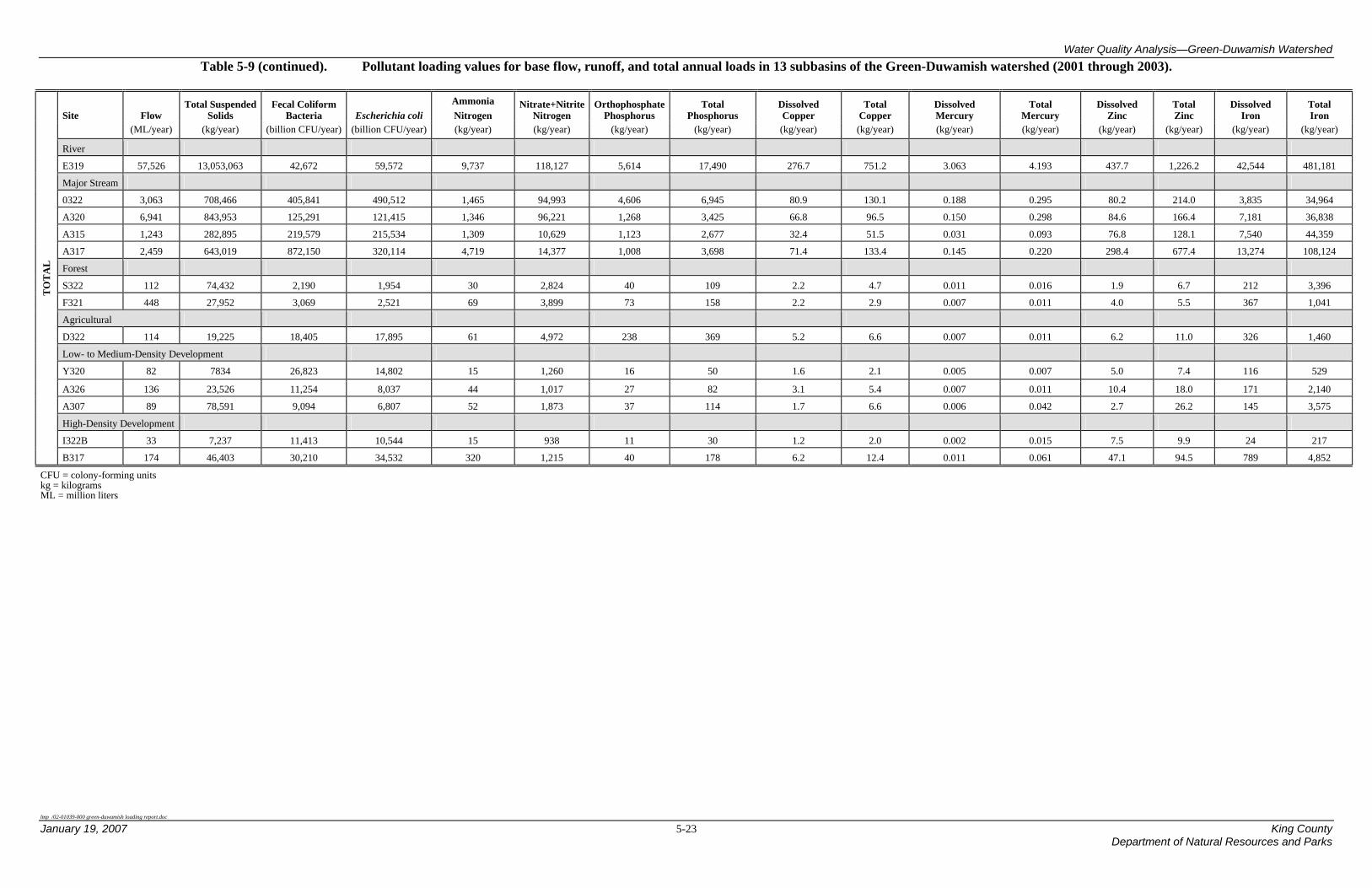
Water Quality Analysis—Green-Duwamish Watershed Table 5-9 (continued). Pollutant loading values for base flow, runoff, and total annual loads in 13 subbasins of the Green-Duwamish watershed (2001 through 2003).








Total Phosphorus

Dissolved Copper

Total Copper

Dissolved Mercury

Total Mercury

Dissolved Zinc

Total Zinc

Dissolved Iron

Total Iron

(ML/year) (kg/year) (billion CFU/year) (billion CFU/year) (kg/year) (kg/year) (kg/year) (kg/year) (kg/year) (kg/year) (kg/year) (kg/year) (kg/year) (kg/year) (kg/year) (kg/year)

River

E319 57,526 13,053,063 42,672 59,572 9,737 118,127 5,614 17,490 276.7 751.2 3.063 4.193 437.7 1,226.2 42,544 481,181

Major Stream

0322 3,063 708,466 405,841 490,512 1,465 94,993 4,606 6,945 80.9 130.1 0.188 0.295 80.2 214.0 3,835 34,964

A320 6,941 843,953 125,291 121,415 1,346 96,221 1,268 3,425 66.8 96.5 0.150 0.298 84.6 166.4 7,181 36,838

A315 1,243 282,895 219,579 215,534 1,309 10,629 1,123 2,677 32.4 51.5 0.031 0.093 76.8 128.1 7,540 44,359

A317 2,459 643,019 872,150 320,114 4,719 14,377 1,008 3,698 71.4 133.4 0.145 0.220 298.4 677.4 13,274 108,124

Forest

S322 112 74,432 2,190 1,954 30 2,824 40 109 2.2 4.7 0.011 0.016 1.9 6.7 212 3,396

F321 448 27,952 3,069 2,521 69 3,899 73 158 2.2 2.9 0.007 0.011 4.0 5.5 367 1,041

Agricultural

D322 114 19,225 18,405 17,895 61 4,972 238 369 5.2 6.6 0.007 0.011 6.2 11.0 326 1,460


Y320 82 7834 26,823 14,802 15 1,260 16 50 1.6 2.1 0.005 0.007 5.0 7.4 116 529

A326 136 23,526 11,254 8,037 44 1,017 27 82 3.1 5.4 0.007 0.011 10.4 18.0 171 2,140

A307 89 78,591 9,094 6,807 52 1,873 37 114 1.7 6.6 0.006 0.042 2.7 26.2 145 3,575


I322B 33 7,237 11,413 10,544 15 938 11 30 1.2 2.0 0.002 0.015 7.5 9.9 24 217

TO

TA

L

B317 174 46,403 30,210 34,532 320 1,215 40 178 6.2 12.4 0.011 0.061 47.1 94.5 789 4,852

CFU = colony-forming units kg = kilograms ML = million liters




Table 5-10. Ratio of annual pollutant runoff loading to base flow loading in 13 subbasins of the Green-Duwamish watershed (2001 through 2003).





Nitrate+Nitrite Nitrogen


Total Phosphorus

Dissolved Copper

Total Copper

Dissolved Mercury

Total Mercury

Dissolved Zinc

Total Zinc

Dissolved Iron

Total Iron

River

E319 0.3 3.6 2.9 2.9 0.4 0.5 0.3 1.2 0.3 2.0 0.3 0.8 0.4 1.8 0.4 2.7

Major Stream

0322 0.3 4.5 11.0 11.4 2.3 0.3 1.9 2.0 1.0 1.5 0.5 1.0 1.2 2.2 0.8 3.7

A320 0.2 1.8 3.7 3.5 0.2 0.1 0.4 0.9 0.5 1.0 0.7 1.0 0.6 1.2 0.5 1.4

A315 0.6 1.5 6.4 15.0 0.6 0.6 2.0 1.9 1.3 1.4 1.4 1.4 1.2 1.2 0.3 0.5

A317 1.0 2.4 38.4 14.5 0.0 0.9 0.3 1.0 2.4 3.0 1.3 2.1 1.7 3.0 0.4 0.7

Forest

S322 0.6 4.8 1.4 1.0 0.4 1.1 0.2 0.9 1.3 2.0 0.7 1.3 0.9 2.5 1.1 5.2

F321 0.2 3.8 6.8 4.1 0.2 0.3 0.1 0.9 0.3 1.1 1.0 1.2 0.5 1.7 0.3 2.6

Agriculture

D322 0.7 2.5 40.6 34.9 3.9 0.7 7.4 4.2 1.8 2.0 1.0 1.5 2.1 2.7 0.6 1.7


Y320 1.8 3.5 26.4 14.3 2.2 2.9 5.8 5.2 3.5 3.8 2.4 3.0 4.1 3.5 1.2 2.2

A326 0.9 3.1 3.4 2.2 2.8 2.1 0.5 1.5 1.5 2.4 1.1 1.7 2.2 2.5 0.5 6.0

A307 0.4 15.3 3.8 4.4 2.2 0.6 0.8 1.8 2.5 7.1 1.3 9.8 2.0 11.3 0.7 7.0


I322B 4.9 27.1 64.1 52.3 17.7 4.0 9.7 12.6 6.3 9.2 6.6 44.1 5.0 5.7 4.9 20.5

B317 2.1 4.4 2.4 1.9 0.3 1.1 1.7 2.1 4.6 5.3 2.9 15.4 4.2 5.2 0.4 1.3

Average 0.6 3.8 6.4 4.4 0.6 0.7 0.8 1.9 1.8 2.0 1.2 1.5 1.6 2.7 0.5 2.6




During runoff, the areal hydraulic loading pattern among the sites was reversed with developed sites producing the most water per hectare (low- to medium-density development = 0.18 ML/ha/year, high-density development = 0.48 ML/ha/year) and rural sites producing the least (agricultural = 0.12 ML/ha/year, forested = 0.11 ML/ha/year) (Table 5-12). This pattern is related to the presence of impervious surfaces in the developed areas that act to increase runoff and decrease base flow. In urban areas, pollutants from anthropogenic byproducts and wastes are readily transported during storm events. There is frequently little processing of these constituents during transport because, in developed areas, flow paths tend to be simplified, with minimal contact time between stormwater and pollutant-retentive soils. Consequently, the presence of impervious area leads to both an increase in runoff volume and pollutant concentrations. In this data set, the result of these processes was evident; runoff areal loading rates for TSS, bacteria, and metals from developed areas were substantially greater than those from undeveloped areas (Table 5-12). Although areal hydraulic loading rates were greater in developed areas than in agricultural areas, runoff areal loading rates of nutrients were greatest from agricultural lands (Table 5-12), where source areas tend to be larger and more concentrated than those in urban areas.

Analysis of total annual areal loading rates is by definition a combination of base flow areal loading rates and runoff areal loading rates. For certain constituents, like nitrate+nitrite nitrogen, the differences noted above between areal loading rates for urban and forested areas in the base flow and runoff, respectively, were not present in the data from the total load analysis. This was due to the fact that nitrate+nitrite nitrogen concentrations were elevated during base flow in forested areas and elevated during storm flow in urban areas; when the base flow and runoff loads were summed, the result was a similar annual load in forested basins (7.7 kilograms per hectare per year [kg/ha/year]), low- to medium-density development (5.9 kg/ha/year) and high-density development (7.6 kg/ha/year) (Table 5-12). Because this analysis segregated loadings into runoff and base flow, the similarity in annual nitrate+nitrite nitrogen loading among these disparate land use categories could be explained.

For metals, ammonia nitrogen, bacteria, and TSS, annual areal loading rates were greatest in high-density development basins (Table 5-12). Areal loadings of nitrate+nitrite nitrogen, orthophosphate phosphorus, and total phosphorus were greatest in agricultural subbasins, but unexpectedly, areal loading rates of TSS were the lowest in agricultural subbasins. This was likely due to the fact that agriculture in the Green-Duwamish watershed is dominated by grazing instead of row crops. Row crops have the potential to export large quantities of sediment, whereas grazing practices generally have a less severe impact on sediment export. The highest areal loading of sediment (381.5 kg/ha/yr) among the sites analyzed originated from site A307 (Hamm Creek), a low-density residential site, while the lowest total annual areal load (40.4 kg/ha/yr) came from site Y320 (Soosette Creek), which is another low-density residential site (Table 5-11). This indicates that these broad land use categorizations can include considerable variability in relation to constituent loading and that groupings, as presented in Table 5-12, should be used carefully with this variability in mind. On an areal basis, forested subbasins exported the lowest concentrations of metals, bacteria, and total phosphorus, while low- to medium-density development subbasins exported the lowest concentrations of nitrate+nitrite nitrogen and orthophosphate phosphorus.




5.2.3 Comparison of Land Use Loading Factors to Literature Values

A comparison of areal loading rates calculated from this data set (Green-Duwamish) and areal loading rates from the literature and from previous King County modeling efforts is presented in Table 5-13. Loading rates from low- to medium-density development and forested subbasins were nearly always higher in the Green-Duwamish data set when compared with the literature values. This may be due to the fact that the Puget Sound area has a higher annual precipitation total relative to the national average and/or the region’s glacial drift soils are highly erodible. Both of these factors could contribute to areal loading rates that are high in comparison to those measured outside the region.

The processes controlling constituent export in forested basins are relatively simple: soil stability, climate, and vegetation. In agricultural areas, there are a wide variety of factors that influence constituent export, including crop type, conservation tillage practices, and grazing and feeding practices. Likewise, high-density development can range from single-family homes on 8-per-acre lots to high-rise apartment buildings. Therefore, much more variability in areal loading is expected from the high-density development and agricultural subbasins than from forested subbasins. Indeed, despite the possible influence of rainfall and erodible soils described above, the areal loading rates for TSS in the high-density development basins and agricultural areas were lower in the Green-Duwamish data set than in the literature (Table 5-13).

Bacterial loading rates for agricultural areas in the Green-Duwamish data set were higher than those found in the literature but lower than those from previous King County modeling efforts (Table 5-13). Bacterial loading rates for the high-density development, low- to medium-density development, and forested subbasins were not substantially different between the previous King County data and Green-Duwamish data sets. Among the three data sets, loading of fecal coliform bacteria was lowest in the literature data set (no E. coli loading data were found in the literature).

Similarly, nutrient loading rates in the King County and Green-Duwamish data sets were generally higher than those in the literature. The one exception was the total phosphorus area loading rate from high-density development areas; this value was 75 and 100 percent higher in the literature data set compared with the Green-Duwamish and King County data, respectively. King County and Green-Duwamish nutrient loading values for the low- to medium-density development, high-density development, and forested land use/cover categories differed by a factor of no more than three (Table 5-13). The results indicate that phosphorus loading from agricultural sources is greater than from urban sources, a finding which is in agreement with studies by Brett et al. (2005a, 2005b).




Table 5-11. Areal pollutant loading values for base flow, runoff, and total annual loads in 13 subbasins of the Green-Duwamish watershed (2001 through 2003).

Site Fecal Coliform




Total Phosphorus

Dissolved Copper Total Copper Dissolved Mercury Total Mercury Dissolved Zinc Total Zinc


Discharge

(ML/ha/year)

Total Suspended Solids

(kg/ha/year) (billion CFU/ha/year) (billion CFU/ha/year) (kg/ha/year) (kg/ha/year) (kg/ha/year) (kg/ha/year) (kg/ha/year) (kg/ha/year) (kg/ha/year) (kg/ha/year) (kg/ha/year) (kg/ha/year) (kg/ha/year) (kg/ha/year)

River E319 0.78 50.4 0.2 0.3 0.126 1.4 0.08 0.14 0.004 0.005 4.04E-05 4.19E-05 0.0056 0.0078 0.56 2.27

Major Stream 0322 0.34 19.0 5.0 5.8 0.065 10.6 0.23 0.34 0.006 0.008 1.87E-05 2.11E-05 0.0054 0.0099 0.31 1.10 A320 0.37 18.7 1.7 1.7 0.069 5.4 0.06 0.11 0.003 0.003 5.62E-06 9.28E-06 0.0032 0.0048 0.31 0.95 A315 0.25 36.1 9.6 4.3 0.262 2.2 0.12 0.30 0.005 0.007 4.22E-06 1.27E-05 0.0111 0.0190 1.93 9.65 A317 0.22 32.9 3.8 3.5 0.778 1.3 0.13 0.32 0.004 0.006 1.09E-05 1.24E-05 0.0193 0.0289 1.68 11.13 Forest S322 0.14 25.9 1.8 1.9 0.045 2.7 0.07 0.11 0.002 0.003 1.27E-05 1.41E-05 0.0020 0.0039 0.20 1.09 F321 0.97 14.5 1.0 1.2 0.138 7.7 0.16 0.21 0.004 0.003 9.29E-06 1.28E-05 0.0069 0.0052 0.69 0.72

Agriculture D322 0.18 14.3 1.2 1.3 0.033 7.5 0.07 0.19 0.005 0.006 9.07E-06 1.13E-05 0.0053 0.0077 0.53 1.43

Low- to Medium-Density Development Y320 0.15 9.0 5.0 5.0 0.024 1.7 0.01 0.04 0.002 0.002 7.63E-06 9.13E-06 0.0050 0.0085 0.27 0.85 A326 0.15 12.5 5.7 5.6 0.025 0.7 0.04 0.07 0.003 0.003 7.04E-06 8.64E-06 0.0070 0.0112 0.25 0.67 A307 0.31 23.3 9.2 6.1 0.079 5.6 0.10 0.20 0.002 0.004 1.23E-05 1.88E-05 0.0045 0.0103 0.42 2.17

High-Density Development I322B 0.05 2.1 1.4 1.6 0.007 1.6 0.01 0.02 0.001 0.002 2.61E-06 2.68E-06 0.0103 0.0122 0.03 0.08

BA

SE F

LO

W

B317 0.34 52.6 53.7 74.0 1.466 3.5 0.09 0.35 0.007 0.012 1.78E-05 2.29E-05 0.0555 0.0929 3.44 12.65 River

E319 0.24 180.6 0.6 0.8 0.046 0.7 0.02 0.17 0.001 0.009 1.38E-05 3.23E-05 0.0021 0.0139 0.20 6.24

Major Stream

0322 0.11 84.9 54.6 66.1 0.150 3.3 0.44 0.68 0.006 0.011 8.87E-06 2.21E-05 0.0064 0.0214 0.25 4.02

A320 0.06 34.1 6.2 5.9 0.015 0.6 0.02 0.10 0.001 0.003 3.79E-06 9.37E-06 0.0021 0.0056 0.14 1.36

A315 0.15 55.3 61.3 65.3 0.160 1.2 0.24 0.57 0.006 0.010 5.88E-06 1.75E-05 0.0137 0.0224 0.51 4.68

A317 0.21 77.7 146.2 51.5 0.034 1.1 0.04 0.31 0.009 0.017 1.4E-05 2.55E-05 0.0320 0.0877 0.60 7.47

Forest

S322 0.08 123.3 2.6 2.0 0.016 3.0 0.01 0.10 0.002 0.006 8.35E-06 1.9E-05 0.0017 0.0096 0.22 5.72

F321 0.15 55.5 6.7 5.1 0.034 2.1 0.02 0.18 0.001 0.004 9.03E-06 1.56E-05 0.0032 0.0086 0.23 1.89

Agriculture

D322 0.12 36.1 47.1 45.6 0.127 5.5 0.55 0.78 0.009 0.012 9.04E-06 1.75E-05 0.0111 0.0211 0.32 2.39


Y320 0.27 31.4 133.4 71.4 0.053 4.8 0.07 0.22 0.006 0.009 1.83E-05 2.71E-05 0.0208 0.0297 0.33 1.88

A326 0.14 39.1 19.0 12.1 0.070 1.5 0.02 0.11 0.004 0.008 7.51E-06 1.51E-05 0.0158 0.0284 0.13 4.02

A307 0.12 358.2 35.0 27.0 0.172 3.5 0.08 0.36 0.006 0.028 1.56E-05 0.000185 0.0087 0.1170 0.28 15.18


I322B 0.23 57.6 92.8 85.4 0.121 6.2 0.08 0.23 0.009 0.015 1.72E-05 0.000118 0.0518 0.0692 0.16 1.71

RU

NO

FF

B317 0.72 231.5 131.3 137.4 0.493 4.0 0.15 0.74 0.031 0.064 5.15E-05 0.000352 0.2331 0.4859 1.39 17.06

Water Quality Analysis—Green-Duwamish Watershed Table 5-11 (continued). Areal pollutant loading values for base flow, runoff, and total annual loads in 13 subbasins of the Green-Duwamish watershed (2001 through 2003).



River E319 1.02 230.9 0.8 1.1 0.172 2.1 0.10 0.31 0.005 0.013 5.42E-05 7.42E-05 0.0077 0.0217 0.75 8.51

Major Stream 0322 0.45 103.9 59.5 71.9 0.215 13.9 0.68 1.02 0.012 0.019 2.75E-05 4.33E-05 0.0118 0.0314 0.56 5.13 A320 0.43 52.8 7.8 7.6 0.084 6.0 0.08 0.21 0.004 0.006 9.4E-06 1.87E-05 0.0053 0.0104 0.45 2.30 A315 0.40 91.4 70.9 69.6 0.423 3.4 0.36 0.86 0.010 0.017 1.01E-05 3.02E-05 0.0248 0.0414 2.44 14.33 A317 0.42 110.6 150.0 55.1 0.812 2.5 0.17 0.64 0.012 0.023 2.49E-05 3.79E-05 0.0513 0.1165 2.28 18.60 Forest S322 0.22 149.2 4.4 3.9 0.061 5.7 0.08 0.22 0.004 0.009 2.11E-05 3.3E-05 0.0037 0.0135 0.42 6.81 F321 1.12 70.0 7.7 6.3 0.172 9.8 0.18 0.40 0.006 0.007 1.83E-05 2.83E-05 0.0101 0.0138 0.92 2.61

Agriculture D322 0.30 50.4 48.2 46.9 0.159 13.0 0.62 0.97 0.014 0.017 1.81E-05 2.88E-05 0.0164 0.0288 0.85 3.83

Low- to Medium-Density Development Y320 0.42 40.4 138.4 76.4 0.077 6.5 0.08 0.26 0.008 0.011 2.59E-05 3.63E-05 0.0258 0.0382 0.60 2.73 A326 0.30 51.7 24.7 17.6 0.096 2.2 0.06 0.18 0.007 0.012 1.45E-05 2.37E-05 0.0229 0.0396 0.38 4.70 A307 0.43 381.5 44.1 33.0 0.251 9.1 0.18 0.55 0.008 0.032 2.79E-05 0.000204 0.0132 0.1273 0.70 17.35

High-Density Development I322B 0.28 59.8 94.2 87.1 0.128 7.7 0.09 0.25 0.010 0.017 1.98E-05 0.000121 0.0621 0.0814 0.20 1.79

TO

TA

L

B317 1.06 284.1 185.0 211.4 1.958 7.4 0.24 1.09 0.038 0.076 6.93E-05 0.000375 0.2886 0.5788 4.83 29.71

CFU = colony-forming units ha = hectare kg = kilograms ML = million liters

Site Fecal Coliform




Total Phosphorus

Dissolved Copper Total Copper Dissolved Mercury Total Mercury Dissolved Zinc Total Zinc


Discharge

(ML/ha/year)

Total Suspended Solids

(kg/ha/year) (billion CFU/ha/year) (billion CFU/ha/year) (kg/ha/year) (kg/ha/year) (kg/ha/year) (kg/ha/year) (kg/ha/year) (kg/ha/year) (kg/ha/year) (kg/ha/year) (kg/ha/year) (kg/ha/year) (kg/ha/year) (kg/ha/year)




Table 5-12. Areal pollutant loading values for base flow, runoff, and total annual loads in tributary subbasins representative of land use/cover categories in the Green-Duwamish watershed (2001 through 2003).

Discharge Total

Suspended Solids

Fecal Coliform Bacteria Escherichia coli Ammonia

Nitrogen Nitrate+Nitrite

Nitrogen Orthophosphate

Phosphorus Total

PhosphorusDissolved Copper Total Copper Dissolved

Mercury Total

Mercury Dissolved

Zinc Total Zinc Dissolved Iron Total Iron

Land Use/Land Cover (ML/ha/year) (kg/ha/year) (billion (CFU/ha/year)

(billion (CFU/ha/year) (kg/ha/year) (kg/ha/year) (kg/ha/year) (kg/ha/year) (kg/ha/year) (kg/ha/year) (kg/ha/year) (kg/ha/year) (kg/ha/year) (kg/ha/year) (kg/ha/year) (kg/ha/year)

Low- to Medium-Density Development 0.20 15.0 6.6 5.5 0.0 2.7 0.05 0.10 0.0024 0.0032 8.99E-06 1.22E-05 0.006 0.010 0.3 1.2

High-Density Development 0.19 27.3 27.6 37.8 0.7 2.5 0.05 0.18 0.0041 0.0068 1.02E-05 1.28E-05 0.033 0.053 1.7 6.4

Agriculture 0.18 14.3 1.2 1.3 0.0 7.5 0.07 0.19 0.0049 0.0058 9.07E-06 1.13E-05 0.005 0.008 0.5 1.4 BA

SE F

LO

W

Forest 0.56 20.2 1.4 1.6 0.1 5.2 0.11 0.16 0.0030 0.0032 1.10E-05 1.34E-05 0.004 0.005 0.4 0.9



Agriculture 0.12 36.1 47.1 45.6 0.1 5.5 0.55 0.78 0.0088 0.0115 9.04E-06 1.75E-05 0.011 0.021 0.3 2.4 RU

NO

FF

Forest 0.11 89.4 4.6 3.5 0.0 2.5 0.02 0.14 0.0019 0.0050 8.69E-06 1.73E-05 0.002 0.009 0.2 3.8



Agriculture 0.30 50.4 48.2 46.9 0.2 13.0 0.62 0.97 0.0136 0.0174 1.81E-05 2.88E-05 0.016 0.029 0.9 3.8 TO

TA

L

Forest 0.67 109.6 6.0 5.1 0.1 7.7 0.13 0.31 0.0050 0.0083 1.97E-05 3.07E-05 0.007 0.014 0.7 4.7

CFU = colony-forming units ha = hectare kg = kilograms ML = million liters




Table 5-13. Comparison of areal loading rates calculated from the Green-Duwamish watershed assessment to areal loading rates from the literature and previous King County studies.

Flow Total

Suspended Solids

Fecal Coliform Bacteria

Escherichia coli

Ammonia Nitrogen



Total Phosphorus

Dissolved Copper Total Copper Dissolved

Mercury Total

Mercury Dissolved

Zinc Total Zinc Dissolved Iron Total Iron

Land Use/Cover (ML/ha/year) (kg/ha/year) (billion

CFU/ha/year) (billion

CFU/ha/year) (kg/ha/year) (kg/ha/year) (kg/ha/year) (kg/ha/year) (kg/ha/year) (kg/ha/year) (kg/ha/year) (kg/ha/year) (kg/ha/year) (kg/ha/year) (kg/ha/year) (kg/ha/year)


GDWQA a 0.38 157.9 69.1 42.4 0.1 5.9 0.11 0.33 0.0078 0.0182 2.28E-05 8.79E-05 0.021 0.068 0.6 8.3

Previous King County data b NA NA 81.7 51.4 0.36 9 0.29 0.32 NA 0.0466 NA NA NA NA NA NA

Literature values c NA 10.0 9.3 NA 0.02 0.1 NA 0.04 NA 0.0100 NA NA NA 0.040 NA NA


GDWQA a 0.67 171.9 139.6 149.2 1.0 7.6 0.17 0.67 0.0241 0.0462 4.46E-05 2.48E-04 0.175 0.330 2.5 15.8


Literature values c NA 420.0 21.0 NA 0.8 2.0 NA 1.00 NA 0.0300 NA NA NA 0.700 NA NA

Agriculture

GDWQA a 0.30 50.4 48.2 46.9 0.2 13.0 0.62 0.97 0.0136 0.0174 1.81E-05 2.88E-05 0.016 0.029 0.9 3.8


Literature values c NA 343.0 16.0 NA 0.7 0.6 0.25 0.58 NA 0.0300 NA NA NA 0.100 NA NA

Forest

GDWQA 0.67 109.6 6.0 5.1 0.1 7.7 0.13 0.31 0.0050 0.0083 1.97E-05 3.07E-05 0.007 0.014 0.7 4.7


Literature values c NA 3.0 4.0 NA NA 0.3 NA 0.03 NA 0.0300 NA NA NA 0.020 NA NA

Literature data sources: Horner et al. (1994); Madison et al. (1979). King County data source: Burkey (2006). CFU = colony-forming units ha = hectare kg = kilograms ML = million liters NA = not available a This study b Burkey (2006) c Horner et al (1994); Burton and Pitt (2002); Madison et al (1979)




Only limited comparisons of areal loading rates for metals could be made because of the limited data available from previous King County modeling efforts and the literature. Compared with the values in other data sets, total copper areal loading rates from the agricultural and forested land use/cover categories were lower in the Green-Duwamish data set. Across all land use/cover categories, total copper areal loading rates were greatest in the King County data set. There were no data for total zinc available from King County; therefore, only comparisons to literature values could be made. Total zinc areal loading rates in the Green-Duwamish and literature data sets were comparable for low- to medium-density development and forest, but the Green-Duwamish values were higher for agricultural and lower for high-density development (Table 5-13).

Overall, loading values in the previous King County modeling efforts and Green-Duwamish data sets were similar and generally higher than those in the literature. Variability between the King County and Green-Duwamish loading data was greatest for the agricultural land use/cover category. This may be explained by the fact that only one agricultural site was used in this areal loading analysis. If additional sites had been used, a more representative area loading rate may have been obtained. Despite this difference, the Green-Duwamish data set reports loadings for a number of constituents that are not included in the King County data set. These additional loading values will add more versatility to current water quality models and improve their overall accuracy for predicting water quality impacts from different types of land use.

5.2.4 Land Use Loading Correlation

In this analysis, correlations between the percentage of land use/cover and effective impervious area in 13 subbasins and constituent areal loading were determined using a Kendall’s Tau correlation. The analysis included correlations using total annual pollutant loading, annual base flow loading, and annual runoff loading. Separate correlation matrices were developed using whole subwatershed land use/cover, 200-meter buffer land use/cover, and 200-meter by 1,000-meter buffer land use/cover. All analyses were run twice: once with data from tributary watersheds and once with data from major stream and tributary watersheds combined. The initial results indicated that using tributary sites alone in the analysis resulted in an unacceptability low n value, thereby reducing the number of significant correlations between land use and constituent areal loading. Likewise, use of the 200-meter by 1,000-meter buffer area did not provide adequate representation of the land use for each monitoring site (i.e., all upland land use/cover categories were excluded from the analysis), thereby reducing the n-value and thus the power of the analysis. Consequently, correlation matrices derived using the 200-meter by 1,000-meter buffer zone and the tributary-only analysis did not provide meaningful information and were excluded from this report. Finally, bare ground had no significant correlation with any of the constituents; therefore, it was excluded from the analysis.

The results of this analysis are summarized in separate subsections below for the following analyses: correlations with whole watershed land use and correlations with 200-meter buffer land use.




5.2.4.1 Correlations of Whole Watershed Land Use/Cover with Annual Constituent Loads

The results of the whole watershed analysis indicated a number of significant correlations between the land use/cover category and constituent loading. Correlations between total annual constituent loadings and land use/cover categories showed that commercial/industrial, high-density residential, agriculture, and effective impervious area were those land use characteristics that were most consistently associated with increased pollutant loading (Table 5-14). Conversely, forest and low-density residential were the land use/cover categories most consistently negatively correlated with pollutant loading. Commercial/industrial land use exhibited significant positive correlations with ammonia nitrogen, total zinc, and dissolved iron. The high-density residential land use/cover category had positive and significant correlations with fecal coliform bacteria and dissolved zinc. Agriculture was most strongly correlated with orthophosphate phosphorus, total phosphorus, and dissolved copper. Effective impervious area showed significant positive correlations with E. coli, ammonia nitrogen, total copper, total mercury, and total and dissolved zinc. Also of interest was a positive correlation between the percentage of roads (areal coverage) within a basin and dissolved zinc (Table 5-14).

Forested land cover had significant negative correlations with fecal coliform bacteria, E. coli, dissolved copper, and total and dissolved zinc (Table 5-14). Negative correlations were also observed between the low-density residential land use/cover category and orthophosphate phosphorus, total phosphorus, dissolved copper, and dissolved iron. Lastly, open water (areal coverage) was negatively correlated with orthophosphate phosphorus. However, this correlation between open water and orthophosphate phosphorus may not be causal; water showed a significant negative correlation with agriculture (Table 5-15), and agriculture showed a significant positive correlated with orthophosphate phosphorus. Consequently, the negative correlation between water and orthophosphate phosphorus may simply be due to the fact that there was very little ground categorized as water in the orthophosphate-enriched agricultural areas.

The results of the base flow loading land use correlations were, for the most part, similar to the results obtained using total annual loading. Commercial/industrial land use was positively correlated with metals and ammonia nitrogen; roads were positively correlated with zinc; forested land cover was negatively correlated with metals; and effective impervious area was positively correlated with E. coli, copper, zinc, and mercury. However, when base flow loadings were used in the analysis, low-density residential land use became negatively correlated with numerous constituents: TSS, nitrate+nitrite nitrogen, orthophosphate phosphorus, total phosphorus, dissolved and total copper, total mercury, and dissolved and total iron. In addition, high-density residential land use was no longer correlated with fecal coliform bacteria and dissolved zinc. Finally, the analysis of base flow loadings showed that grass/crops/shrubs became positively correlated with bacteria, whereas dry/native grass became negatively correlated with TSS and total mercury.




Table 5-14. Kendall’s Tau correlations between total watershed land use/cover and annual constituent loading in the major streams and tributaries of the Green-Duwamish watershed.

n Total

Suspended Solids

Fecal Coliform Bacteria

Escherichia coli

Ammonia Nitrogen

Nitrate+Nitrite

Nitrogen

Orthophosphate

Phosphorus

Total Phosphorus

Dissolved Copper Total Copper Dissolved

Mercury Total

Mercury Dissolved Zinc Total Zinc Dissolved Iron Total Iron

Correlation with Total Annual Load

Low-density residential 11 0.02 -0.02 -0.02 -0.33 -0.33 -0.56 -0.69 -0.47 -0.07 -0.07 0.16 0.20 0.20 -0.51 -0.16

High-density residential 7 -0.33 0.62 0.43 0.43 -0.05 0.05 -0.05 0.33 -0.24 0.05 0.05 0.62 -0.05 0.24 -0.24

Commercial/industrial 9 0.44 0.39 0.17 0.72 -0.11 0.22 0.44 0.44 0.39 0.11 0.28 0.44 0.56 0.50 0.44

Agriculture 6 0.07 -0.20 0.07 0.20 0.33 0.87 0.87 0.73 0.33 0.33 -0.07 -0.20 -0.20 0.33 0.07

Forest 13 0.12 -0.79 -0.73 -0.39 -0.30 -0.21 -0.30 -0.58 -0.33 -0.12 -0.30 -0.88 -0.48 -0.30 -0.06

Grass/crops/shrubs 13 -0.06 0.30 0.30 0.15 0.12 0.09 0.18 0.09 0.15 0.06 0.06 0.21 0.30 0.18 0.06

Dry/native grass 13 -0.36 0.06 0.00 -0.21 0.00 -0.09 -0.06 -0.03 0.03 -0.30 -0.24 0.09 0.12 -0.06 -0.12

Wetlands 12 0.02 -0.09 -0.24 0.31 -0.31 0.13 0.13 -0.09 0.05 -0.27 -0.24 -0.13 -0.05 0.27 0.20

Water 9 -0.07 -0.14 -0.36 -0.21 -0.43 -0.71 -0.43 -0.29 -0.07 -0.43 -0.29 0.00 0.00 -0.21 0.14

Roads 13 -0.12 0.42 0.42 0.21 0.06 0.03 0.06 0.27 0.21 -0.12 0.18 0.58 0.42 0.12 -0.06

Effective impervious area 12 0.25 0.55 0.62 0.47 0.55 0.33 0.40 0.62 0.62 0.25 0.76 0.69 0.84 0.11 0.18

Correlation with Annual Base Flow Load

Low-density residential 11 -0.51 -0.11 -0.11 -0.42 -0.56 -0.60 -0.64 -0.82 -0.73 -0.33 -0.56 -0.07 0.02 -0.60 -0.51

High-density residential 7 0.24 -0.24 -0.43 0.43 -0.24 0.05 0.05 -0.24 -0.14 -0.43 -0.24 0.33 0.43 0.24 0.33


Agriculture 6 0.07 0.07 0.20 -0.20 0.33 0.33 0.33 0.73 0.60 0.33 0.47 -0.07 -0.07 0.33 0.20

Forest 13 0.12 -0.27 -0.15 -0.03 0.03 -0.03 -0.12 -0.03 -0.09 0.18 0.21 -0.52 -0.61 -0.24 -0.15

Grass/crops/shrubs 13 -0.06 0.52 0.52 0.03 0.03 0.09 0.12 -0.03 0.09 -0.12 -0.03 0.03 0.24 0.12 0.03

Dry/native grass 13 -0.48 0.03 0.03 -0.33 -0.03 -0.33 -0.30 -0.15 -0.21 -0.36 -0.45 -0.15 -0.06 -0.12 -0.27

Wetlands 12 0.27 0.05 -0.05 0.42 -0.13 0.27 0.24 0.20 0.20 -0.13 0.09 0.24 0.13 0.42 0.27

Water 9 -0.36 -0.14 -0.29 -0.07 -0.64 -0.57 -0.50 -0.43 -0.43 -0.36 -0.71 0.07 0.00 -0.21 -0.14

Roads 13 -0.18 0.33 0.15 -0.03 -0.21 -0.15 -0.06 -0.21 -0.09 -0.42 -0.27 0.27 0.48 0.06 -0.03

Effective impervious area 12 -0.11 0.62 0.62 -0.04 0.18 0.11 0.18 0.04 0.11 -0.18 -0.04 0.40 0.76 0.11 0.04

Correlation with Annual Runoff Load

Low-density residential 11 -0.02 -0.02 -0.02 -0.20 0.02 -0.42 -0.56 -0.16 -0.02 0.16 0.24 0.20 0.24 -0.29 -0.07

High-density residential 7 -0.33 0.62 0.43 0.05 0.14 0.14 -0.33 0.52 -0.14 0.43 0.14 0.62 -0.05 0.52 -0.24

Commercial/industrial 9 0.33 0.39 0.17 0.28 0.00 0.11 0.33 0.39 0.44 0.11 0.33 0.44 0.50 0.50 0.44

Agriculture 6 0.20 -0.20 0.07 0.47 0.47 0.87 1.00 0.47 0.20 0.07 -0.07 -0.20 -0.20 0.33 0.20

Forest 13 0.09 -0.79 -0.73 -0.30 -0.48 -0.45 -0.33 -0.73 -0.42 -0.52 -0.36 -0.88 -0.52 -0.48 0.00


Dry/native grass 13 -0.39 0.06 0.00 0.00 0.06 0.09 0.09 0.12 0.06 -0.03 -0.12 0.09 0.15 -0.06 -0.18

Wetlands 12 -0.09 -0.09 -0.24 -0.09 -0.56 -0.05 -0.05 -0.24 -0.05 -0.35 -0.31 -0.13 -0.09 -0.02 0.09

Water 9 -0.14 -0.14 -0.36 -0.43 -0.36 -0.57 -0.36 -0.21 -0.07 -0.36 -0.21 0.00 0.00 -0.29 0.00

Roads 13 -0.15 0.42 0.42 0.24 0.18 0.27 0.15 0.30 0.30 0.21 0.18 0.58 0.39 0.18 -0.06






The same analysis was repeated with runoff loadings and, again, the correlation pattern changed slightly. Low-density residential land use showed only a negative correlation with total phosphorus, whereas commercial/industrial land use was a positive correlation only with total zinc and dissolved iron. Effective impervious area was still positively correlated with total zinc, dissolved zinc, total copper, total mercury, and E. coli bacteria loading, but was not significantly correlated with dissolved copper loading. As with the results of the total annual loading analysis, high-density residential land use was positively correlated with fecal coliform bacteria and dissolved zinc. Agriculture was positively correlated with orthophosphate phosphorus and total phosphorus; and forested land cover was negatively correlated with the majority of bacteria, nutrients, and metals analyzed. Lastly, wetlands were negatively correlated with nitrate+nitrite nitrogen; water was negatively correlated with orthophosphate phosphorus; and roads were positively correlated with dissolved zinc.

The fact that agriculture was only positively correlated with phosphorus species and copper was of interest because past studies have shown agricultural land use to be a primary determinant of suspended sediment (Allan et al. 1997; Johnson et al. 1997), nutrients (Ahearn et al. 2005; Arheimer and Liden 2000; Smart et al. 1998), and bacteria (Mehaffey et al. 2005). Both the principal component analysis and the visual presentation of the data in Appendix B indicate that the agricultural sites were marked by high concentrations of E. coli, fecal coliform bacteria, nitrate+nitrite nitrogen, ammonia nitrogen, orthophosphate phosphorus, total phosphorus, and dissolved iron and copper. However, phosphorus and copper were the only constituents that were positively correlated with agricultural land use in the land use loading analysis. This is primarily because there were no flow data available for site B322 (Newaukum tributary at S.E. 424th Street), which is the agricultural site with the highest pollutant concentrations in the study. Therefore, the data from this site were excluded from the land use loading analysis, and consequently the apparent impact of agricultural land use on pollutant loading was reduced.

5.2.4.2 Correlations of 200-Meter Buffer Land Use/Cover with Annual Constituent Loads

When the percentage of land use coverage was limited to the 200 meters bordering the channel, the correlation patterns between land use/cover category and pollutant loading (Table 5-16) did not change substantially relative to what was observed with the whole watershed land use/cover. Comparisons made between the two analyses showed there were the following differences in the results:

When total annual loadings were used in the analysis, roads showed a positive correlation with E. coli bacteria in addition to the positive correlation with dissolved zinc described above. Furthermore, commercial/industrial land use also showed a positive correlation with TSS in addition to the correlations with ammonia nitrogen, zinc, and iron.

When base flow loadings were used in the analysis, agriculture showed a positive correlation with total copper in addition to the correlation with dissolved copper described above.




When runoff loadings were used in the analysis, roads again showed a positive correlation with E. coli bacteria in addition to the correlation with dissolved zinc described above. And, high-density residential land use no longer showed a significant positive correlation with fecal coliform bacteria and dissolved zinc.

When comparing Tables 3-1 and 3-2, it is difficult to attribute any of the above noted variations in land use loading correlation to differences in land use percent coverage between the whole watershed and 200-meter buffer areas. The tributary sites exhibit minor percent coverage differences, between the whole watershed and 200-meter buffer areas, and no obvious patterns develop which could explain why some of the correlations changed for those areas. The results of this analysis indicate that, after limiting the land use categories used in the analysis to a 200-meter buffer, the correlation between some land use categories and pollutant loading increased, whereas other relationships became insignificant. There was not, however, a clear pattern as to which relationships weakened and which grew stronger. Consequently, the use of both methods (200-meter buffer and whole watershed land use) should be considered in any future analyses.




Table 5-15. Kendall’s Tau correlations among land use/cover categories in the Green-Duwamish watershed.

Low-Density Residential

High-Density Residential

Commercial/ Industrial Agriculture Forest

Grass/Crops/ Shrubs

Dry/Native Grass Wetlands Water Roads


Low-density residential –

High-density residential 0.43 –

Commercial/industrial -0.22 0.33 –

Agriculture -0.87 -0.80 -0.20 –

Forest 0.11 -0.43 -0.28 -0.07 –

Grass/crops/shrubs 0.11 0.05 0.22 -0.07 -0.24 –

Dry/native grass 0.20 0.33 -0.06 0.07 -0.18 0.39 –

Wetlands -0.06 -0.07 0.00 -0.20 0.24 0.38 0.31 –

Water 0.47 -0.07 0.07 -1.00 -0.05 0.05 0.14 0.47 –

Roads 0.42 0.43 0.22 -0.47 -0.39 0.55 0.36 0.05 0.05 –

Effective impervious area 0.09 0.33 0.82 -0.47 -0.47 0.63 0.26 0.15 0.24 0.66 –





Table 5-16. Kendall’s Tau correlations between 200-meter buffer land use/cover and annual constituent loading in the major streams and tributaries of the Green-Duwamish watershed.

n Total Suspended






Total Phosphorus

Dissolved Copper Total Copper

Dissolved Mercury Total Mercury Dissolved Zinc Total Zinc Dissolved Iron Total Iron

Correlation with Total Annual Load

Low-density residential 11 0.02 -0.02 -0.02 -0.33 -0.33 -0.56 -0.69 -0.47 -0.07 -0.07 0.16 0.20 0.20 -0.51 -0.16

High-density residential 7 -0.33 0.43 0.24 0.24 0.14 -0.14 -0.24 0.14 -0.24 0.05 0.05 0.43 -0.05 0.05 -0.24


Agriculture 6 -0.07 -0.33 -0.07 0.07 0.20 0.73 0.73 0.60 0.20 0.20 -0.20 -0.33 -0.33 0.47 0.20

Forest 13 0.18 -0.73 -0.67 -0.39 -0.42 -0.33 -0.42 -0.70 -0.33 0.00 -0.12 -0.76 -0.36 -0.30 -0.06

Grass/crops/shrubs 13 -0.09 0.45 0.39 0.24 0.09 0.06 0.21 0.18 0.18 -0.03 0.03 0.42 0.33 0.33 0.15

Dry/native grass 13 -0.39 0.15 0.03 0.00 0.15 0.06 -0.03 0.12 0.00 -0.15 -0.15 0.12 0.09 0.03 -0.15

Wetlands 12 -0.05 -0.09 -0.24 0.16 -0.24 -0.02 0.05 -0.16 -0.02 -0.35 -0.24 -0.13 -0.05 0.13 0.13

Water 8 -0.05 -0.05 -0.33 -0.14 -0.43 -0.71 -0.43 -0.24 0.05 -0.43 -0.24 0.14 0.14 -0.14 0.33

Roads 13 -0.12 0.42 0.48 0.21 0.12 0.03 0.06 0.27 0.21 -0.06 0.18 0.58 0.42 0.12 -0.06


Correlation with Annual Base Flow Load

Low-density residential 11 -0.51 -0.11 -0.11 -0.42 -0.56 -0.60 -0.64 -0.82 -0.73 -0.33 -0.56 -0.07 0.02 -0.60 -0.51

High-density residential 7 0.05 -0.43 -0.43 0.24 -0.05 -0.14 -0.14 -0.43 -0.33 -0.24 -0.24 0.14 0.24 0.05 0.14


Agriculture 6 0.20 0.20 0.33 -0.07 0.47 0.47 0.47 0.87 0.73 0.47 0.60 -0.20 -0.20 0.47 0.33

Forest 13 0.12 -0.09 -0.03 -0.03 -0.09 -0.09 -0.18 -0.21 -0.21 0.12 0.15 -0.52 -0.48 -0.24 -0.15

Grass/crops/shrubs 13 0.09 0.55 0.42 0.24 -0.06 0.12 0.21 0.06 0.12 -0.21 -0.06 0.24 0.39 0.27 0.18

Dry/native grass 13 -0.33 0.06 0.00 -0.12 0.12 -0.12 -0.09 -0.18 -0.18 -0.27 -0.30 -0.12 0.09 -0.03 -0.06

Wetlands 12 0.13 0.05 -0.05 0.27 -0.13 0.13 0.09 0.05 0.05 -0.20 -0.05 0.16 0.13 0.27 0.13

Water 8 -0.33 -0.05 -0.24 0.05 -0.62 -0.52 -0.52 -0.43 -0.43 -0.43 -0.81 0.24 0.14 -0.14 -0.05

Roads 13 -0.18 0.39 0.21 -0.03 -0.15 -0.15 -0.06 -0.21 -0.09 -0.42 -0.27 0.27 0.48 0.06 -0.03

Effective impervious area 12 0.11 0.56 0.38 0.32 -0.08 0.20 0.29 0.08 0.20 -0.17 -0.08 0.56 0.78 0.26 0.23

Correlation with Annual Runoff Load

Low-density residential 11 -0.02 -0.02 -0.02 -0.20 0.02 -0.42 -0.56 -0.16 -0.02 0.16 0.24 0.20 0.24 -0.29 -0.07

High-density residential 7 -0.33 0.43 0.24 0.05 0.14 -0.05 -0.52 0.52 -0.14 0.43 0.14 0.43 -0.05 0.33 -0.24

Commercial/industrial 9 0.39 0.33 0.11 0.33 0.06 0.06 0.28 0.44 0.50 0.17 0.39 0.39 0.56 0.44 0.50

Agriculture 6 0.07 -0.33 -0.07 0.33 0.33 0.73 0.87 0.33 0.07 -0.07 -0.20 -0.33 -0.33 0.20 0.07

Forest 13 0.15 -0.73 -0.67 -0.36 -0.48 -0.58 -0.52 -0.79 -0.36 -0.39 -0.18 -0.76 -0.39 -0.42 0.00


Dry/native grass 13 -0.42 0.15 0.03 0.09 -0.03 0.18 0.00 0.21 0.03 0.06 -0.03 0.12 0.12 0.09 -0.21

Wetlands 12 -0.16 -0.09 -0.24 -0.16 -0.64 -0.13 -0.13 -0.31 -0.13 -0.42 -0.31 -0.13 -0.09 -0.09 0.02

Water 8 -0.14 -0.05 -0.33 -0.43 -0.33 -0.52 -0.33 -0.14 0.05 -0.33 -0.14 0.14 0.14 -0.24 0.14

Roads 13 -0.15 0.42 0.48 0.30 0.24 0.33 0.15 0.30 0.30 0.27 0.24 0.58 0.39 0.18 -0.06





January 19, 2007 6-1 King County| Department of Natural Resources and Parks

6.0 Conclusions

This report represents a summary of the water quality and flow data collected by King County in the Green-Duwamish watershed from 2001 through 2003. Analyses performed on the data included the following:

A comparison of the routine and GDWQA sampling approaches A comparison of water quality data for base flow and storm flow A hysteresis analysis for TSS and alkalinity A correlation analysis among water quality parameters A correlation analysis between water quality and hydrologic parameters A principal component analysis A correlation analysis between constituent loading and land use/cover

categories.

With each analysis, it was apparent that patterns in the data were strongly influenced by land use/cover patterns. Hence, this section summarizes the conclusions from all of the analyses in relation to three broad land use categories: agricultural land, forested land, and developed areas. Additional conclusions and recommendations regarding sampling strategies, buffer effects, and land use loading comparisons are included in section 7.0.

6.1 Agricultural Land

The loading analysis indicated that agricultural land use was positively correlated with only phosphorus and copper. However, the principal component analysis indicated that the agricultural sites were associated with high concentrations of nitrate+nitrite nitrogen, ammonia nitrogen, E. coli, and fecal coliform bacteria (although conspicuously not TSS). Additionally, the data summaries presented in Appendix B show that the agricultural sites generally had the highest nitrogen concentrations of all the sites. Consequently, it was apparent that the correlation analyses performed on the loading data were not capable of capturing all of the influences on nutrient and bacteria concentrations among the sites. This can be explained by the fact that the site that was most strongly influenced by agricultural land use (site B322) was not used in the loading analysis because flow data were not available for the site. The elevated loading of nutrients and bacteria is likely a result of the grazing practices used within the agricultural basins. Cattle wastes contain nutrients and bacteria, while grazing impacts riparian vegetation and compacts soils. The result is simplified flowpaths from source areas to the stream channel, and increased source area concentrations of bacteria and nutrients.

The analysis of concentration data identified a number of other important patterns in the data from sites with agricultural land use. For example, antecedent dry period was shown to be positively correlated with TSS and negatively correlated with dissolved oxygen at these sites. None of the other land uses showed a similar correlation with antecedent conditions. Additionally, the agricultural sites had the highest ratios of storm flow concentration to base flow




concentration for total phosphorus, orthophosphate phosphorus, and bacteria, and the hysteresis analysis attributed the strongest sediment flushing patterns to these sites. These patterns all indicate that the first-flush effect is evident for TSS, total phosphorus, orthophosphate phosphorus, and bacteria in agricultural areas.

Nitrate+nitrite nitrogen was negatively correlated with average flow in the agricultural basins, an indication that the groundwater in these areas was enriched with nitrate+nitrite nitrogen and was exported in a piston-flow fashion during small storms; a trend that can also be observed in the data summaries presented in Appendix B (see Figure B-12). Finally, because nitrate+nitrite nitrogen and ammonia nitrogen were elevated in base flow and in storm flow (Appendix B), many of the correlations between TSS and nitrogen were not observed. These water quality patterns were manifest in the PCA analysis as agricultural land use sites grouped strongly with bacteria, phosphorus, and nitrogen, among other parameters. Overall, the pattern of water quality data is indicative of grazing-dominated agriculture, whereby livestock contribute to elevated concentrations of bacteria and phosphorus in runoff and elevated nitrogen concentrations in runoff and groundwater. This pattern is distinct from row crop runoff, which is characterized by high sediment concentrations and lower bacteria concentrations.

6.2 Forested Land

The loading analysis indicated that forested lands showed a consistently negative correlation with bacteria, nutrients (when runoff loads were assessed), and metals loadings. The principal component analysis identified the same pattern and also indicated that forested areas were associated with high concentrations of dissolved oxygen. In these undisturbed watersheds, storms were the primary influence on water quality. For example, the analyses showed that TSS was correlated with many metals and nutrients because these constituents were exported together during storm events. The hysteresis analysis showed that the majority of these storm events were characterized by TSS flushing. The TSS concentrations in the storm flow samples were related to the “flashiness” of the event. Overall, the water quality pattern observed in these data is indicative of relatively undisturbed forested watersheds, where base flow is lacking in nutrients and metals and periodic large inputs of stormwater export high levels of sediment and associated solutes.

6.3 Developed Areas

Some of the more complex relationships within this data set were observed in monitoring results from the developed basins. The combination of natural and human-induced influences on water quality lead to a high degree of variability within the data; that is, the complexity of the data structure is a reflection of the complexity of the processes that produced the data. The loading analysis indicated that roads and effective impervious area were correlated with high concentrations of fecal coliform bacteria and total zinc. The zinc is most likely derived from automobile tire wear, while fecal coliform is attributable primarily to pets and urban wildlife (e.g., birds and rodents). Because these areas are impervious, there is minimal biological




processing of runoff before stormwater reaches the channel. Consequently, bacteria which would have otherwise been processed in interflow, are routed directly to the channel.

Roads are most dense in highly developed and commercial land uses. Both highly developed and commercial land uses were also correlated with zinc loading. Commercial/industrial land use was positively correlated with the widest variety of constituents, including bacteria, metals, and ammonia nitrogen. Conversely, low-density residential land use was negatively correlated with nutrient and metals loading. In general, the pattern of constituent export from low- to medium-density residential land use was more similar to that of forested land use than to other developed land uses.

An important distinction exists between low-density residential as a GIS calculated land use versus low- to medium-density residential as a broad categorization for a watershed (e.g., tributary sites Y320, A330, A326, and A307). Although there was no strong relationship between low-density residential land use/cover and pollutant loading, tributary basins labeled “low- to medium-density residential” can be significant sources of pollutants. Indeed, the highest areal loading of sediment (381.5 kg/ha/yr) among the sites analyzed originated from site A307 (Hamm Creek), a low- to medium-density residential site. Conversely, the lowest total annual areal load (40.4 kg/ha/yr) came from Y320 (Soosette Creek), another low- to medium-density residential site. This indicates that these broad land use categorizations can include considerable variability in relation to constituent loading and that a closer inspection of land use practices should be made before grouping these sites in the future.

In all the developed basins, TSS concentrations were positively correlated with the concentrations of total metals, indicating that stormwater runoff is a primary influence on water quality. Indeed, the hysteresis analysis showed a distinction in the data between pollutant-laden stormwater runoff and groundwater discharge. The developed sites exhibited a consistent counterclockwise hysteresis pattern for alkalinity which indicates that concentrations measured on the rising limb of the hydrograph were lower than those measured on the falling limb. Alkalinity concentrations are generally higher in groundwater; therefore, it can be inferred that the falling limb was primarily composed of groundwater, whereas the rising limb was primarily made up of direct runoff from impervious surfaces within the drainage basin. The hysteresis analysis also indicated that there was no sediment-flushing effect in the developed basins. More specifically, the analyses showed there was generally a positive linear relationship between discharge and TSS concentration; however, there was no clockwise hysteresis that would suggest a first-flush effect. This was in contrast to the agricultural and forested sites which showed evidence of TSS source depletion throughout the duration of the majority of the storm events analyzed. Hence, it can be inferred that sediment sources in the developed basins are either large enough or mobile enough to resist depletion through the rising limb of the hydrograph.

Although there was no evidence of a first-flush effect, the analysis did indicate a positive correlation between the antecedent dry period and copper and zinc concentrations in highly developed basins. This would indicate a seasonal hysteresis; that is, the storms early in the season (October through November) are more likely to export more metals than storms which occur later in the season.




7.0 Implications of Study Results

This study summarized, reduced, and interpreted a large water quality data set consisting of more than 1,400 samples each of which were evaluated for 25 parameters. This section discusses the practical implications of the results in terms of monitoring, modeling, and management.

7.1 Implications for Monitoring

7.1.1 Monitoring Site Locations

In any water quality monitoring effort, the interpretation of results requires some knowledge of watershed characteristics including pollutant source areas and landscape alterations that can influence flow regimes. Drawing correlations between lowland river water quality and headwater basin characteristics in large rivers often results in misleading results because of the many diverse influences on water quality that come into play on such a large scale. Instream processing, flow routing, and tributary and point source inputs all contribute to the mosaic of forces that dictate water quality in high-order streams. Therefore, the majority of analyses conducted in this study have excluded the major river sites and focused instead on data from the small tributaries. In these tributaries, the linkage between land use and stream water quality is more easily examined and quantified. This concept should also be considered when selecting monitoring stations such that tributary sites are given priority over main stem sites because more useful information can be obtained from the former.

7.1.2 Sampling Method

Each sampling method used in this study has advantages and disadvantages. Autosamplers are expensive to operate, and in the case of sequential sampling, the laboratory analyses are expensive; however, the analysis of more samples results in a more accurate characterization of water quality. Composite sampling reduces the number of samples while still characterizing the mean concentration of a storm event. The drawback of composite sampling is that peak concentrations are not quantified and maintenance of the autosampler is expensive. Grab sampling is relatively inexpensive, but rigorous storm sampling must be employed in order for the program to be effective.

The assessment of the sampling methods used in this study indicates that auto-sequential sampling is the best method for sampling both storm and base flow in order to evaluate exceedances of water quality standards and to estimate pollutant loading. However, grab sampling is also effective at capturing maximum concentrations and, if a regression approach to load estimation is used in accordance with rigorous storm sampling, grab samples can be used to reliably estimate pollutant loading. For large basins, biweekly sampling is recommended. In addition to the biweekly sampling, a complimentary storm flow sampling program is recommended because the data indicated that storm flow water quality was significantly different




from base flow water quality. Therefore, accurate characterization of watershed water quality cannot be completed without a storm flow sampling program. If budgetary resources are adequate, autosamplers should be used for this effort; however, grab sampling will suffice if a sufficient number of samples are collected to adequately characterize the inherent variability in the data across a range of different storm sizes.

The hysteresis analysis indicated that flushing flows (those with higher concentrations on the rising limb than on the falling limb) occurred for approximately 50 percent of the analyzed storms. This implies that when sampling storm flow, it is important to avoid the inherent tendency to sample more often during the falling limb of the storm because concentrations may be much lower than those on the rising limb or peak of the storm. Hysteresis in stormwater quality can increase uncertainty in grab sampling data sets if the grab samples are biased toward falling limb chemistries. The use of sequential autosampling avoids this issue but at considerable economic expense. Hysteresis in stormwater quality was most consistent from the agricultural site (D322) used in this analysis. This implies that care should be taken when sampling stormwater from watersheds dominated by agriculture.

7.1.3 Constituent Testing

Analysis of correlations among water quality constituents revealed that there are a few parameters that are consistently correlated with each another. Total metals, total phosphorus, TSS, and turbidity were frequently correlated. These same constituents were often inversely correlated with alkalinity, specific conductance, and hardness. This implies that, when budgetary resources are limited, testing could be done for select constituents, and the concentrations of the other constituents could be inferred from the results. However, this is not recommended in situations where the rigorous quantification of water quality is required. Nevertheless, for exploratory sampling purposes, this approach may be useful. An example of this approach is to use turbidity as a surrogate for TSS, and to measure turbidity in situ to provide a continuous record of turbidity and a better estimate of overall TSS loading relative to estimates derived solely from grab samples.

7.2 Implications for Modeling

The results of this analysis have provided site-specific areal loading rates for a suite of 15 constituents. Previous King County water quality models used land use loading factors based on a combination of observational and literature values (Burkey 2006). This study showed that literature values tend to be lower than both the values derived from this study and the values used by King County for previous modeling efforts. This could be due to the fact that the Puget Sound area receives higher annual rainfall than the majority of the country. Consequently, it is important to use regionally derived numbers when estimating pollutant loading from various land use source areas. Additionally, loading factors were previously available for only seven constituents. The data set provided with this report adds an additional eight constituents. The loading factors presented in Table 5-12 will serve as the most accurate estimate of pollutant areal




loading for the Green-Duwamish watershed and surrounding watersheds. Furthermore, these results will allow more accurate projections of pollutant loading dynamics to be made within a rapidly changing demographic setting.

7.3 Implications for Management

7.3.1 Management of Riparian Areas

The land use loading correlation results revealed important relationships between water quality and land use when land use data from both the whole watershed and a 200-meter buffer were applied. This would suggest that the impact of land use practices on water quality is equally important whether the source area is located near a major stream channel or not. That is, increasing the proximity of a land use to the channel does not necessarily result in an increase in pollutant loading. Consequently, land use and water resource management activities that are intended to reduce pollutant loads should not focus only on the riparian zone but should encompass the entire watershed.




8.0 References

Agouridis, C.T., D.R. Edwards, S.R. Workman, J.R. Bicudo, B.K. Koostra, E.S. Vanzant and J.L. Taraba. 2005. Streambank erosion associated with grazing practices in the humid region. Transactions of the Asae, 48(1): 181-190.

Ahearn, D.S., R.W. Sheibley, R.A. Dahlgren, and K.E. Keller. 2004. Temporal Dynamics of Stream Water Chemistry in the Last Free-Flowing River Draining the Western Sierra Nevada, California. Journal of Hydrology 295(1-4):47-63.

Ahearn, D.S., R.W. Sheibley, R.A. Dahlgren, M. Anderson, J. Johnson, and K.W. Tate. 2005. Land Use and Land Cover Influence on Water Quality in the Last Free-Flowing River Draining the Western Sierra Nevada, California. Journal of Hydrology 313(3-4):234-247.

Allan, J.D., D.L. Erickson, and J. Fay. 1997. The Influence of Catchment Land Use on Stream Integrity across Multiple Spatial Scales. Freshwater Biology 37(1):149-161.

APHA, AWWA and WEF. 1998. Standard Methods for the Examination of Water and Wastewater. 20th edition. Edited by L.S. Clesceri, A.E. Greenberg and A.D. Eaton. American Public Health Association, American Water Works Association, and Water Environment Federation, Baltimore, Maryland.

Arheimer, B. and R. Liden. 2000. Nitrogen and Phosphorus Concentrations for Agricultural Catchments; Influence of Spatial and Temporal Variables. Journal of Hydrology 227(1-4):140-159.

Arnold, C.L. and C.J. Gibbons. 1996. Impervious Surface Coverage: the Emergence of a Key Environmental Indicator. American Planning Association Journal 62:243-258.

Barringer, T.H., R.G. Reiser, and C.V. Price. 1994. Potential Effects of Development on Flow Characteristics of 2 New-Jersey Streams. Water Resources Bulletin 30(2):283-295.

Basnyat, P., L.D. Teeter, K.M. Flynn, and B.G. Lockaby. 1999. Relationships between Landscape Characteristics and Nonpoint Source Pollution Inputs to Coastal Estuaries. Environmental Management 23(4):539-549.

Bolstad, P.V. and W.T. Swank. 1997. Cumulative Impacts of Landuse on Water Quality in a Southern Appalachian Watershed. Journal of the American Water Resources Association 33(3):519-533.

Booth, D.B. and C.R. Jackson. 1997. Urbanization of Aquatic Systems: Degradation Thresholds, Stormwater Detection, and the Limits of Mitigation. Journal of the American Water Resources Association 33(5):1077-1090.

Boyd, M.J., M.C. Bufill, and R.M. Knee. 1993. Pervious and Impervious Runoff in Urban Catchments. Hydrological Sciences Journal-Journal Des Sciences Hydrologiques 38(6):463-478.




Brett, M.T., G.B. Arhonditsis, S.E. Mueller, D.M. Hartley, J.D. Frodge and D.E. Funke. 2005a. Non-point-source impacts on stream nutrient concentrations along a forest to urban gradient. Environmental Management, 35(3): 330-342.

Brett, M.T., S.E. Mueller and G.B. Arhonditsis. 2005b. A daily time series analysis of stream water phosphorus concentrations along an urban to forest gradient. Environmental Management, 35(1): 56-71.

Burkey, Jeff. 2006. Personal communication (email message to Dylan Ahearn, Herrera Environmental Consultants, Seattle, Washington, regarding King County land use loading estimates). Hydrologist, King County Water and Land Resources Division, Seattle, Washington. October 4, 2006.

Burton, G.A. and R. Pitt. 2002. Stormwater Effects Handbook: A Toolbox for Watershed Managers, Scientists, and Engineers. Lewis Publishers, Boca Raton, Florida.

Buttle, J.M. 1994. Isotope Hydrograph Separations and Rapid Delivery of Pre-Event Water from Drainage Basins. Progress in Physical Geography 18(1):16-41.

Collins, R. and A. Jenkins. 1996. The Impact of Agricultural Land Use on Stream Chemistry in the Middle Hills of the Himalayas, Nepal. Journal of Hydrology 185(1-4):71-86.

Creed, I.F. and L.E. Band. 1998. Export of Nitrogen from Catchments within a Temperate Forest: Evidence for a Unifying Mechanism Regulated by Variable Source Area Dynamics. Water Resources Research 34(11):3105-3120.

Durum, W.H. 1953. Relationship of the Mineral Constituents in Solution to Stream Flow, Saline River near Russell, Kansas. Transactions, American Geophysical Union 34(3):435-442.

Ecology. 1995. 1994 Washington State Water Quality Assessment. Washington State Department of Ecology, Olympia, Washington.

Gremillion, P., A. Gonyeau, and M. Wanielista. 2000. Application of Alternative Hydrograph Separation Models to Detect Changes in Flow Paths in a Watershed Undergoing Urban Development. Hydrological Processes 14(8):1485-1501.

Harriman, R., E. Gillespie, D. King, A.W. Watt, A.E.G. Christie, A.A. Cowan, and T. Edwards. 1990. Short-Term Ionic Responses as Indicators of Hydrochemical Processes in the Allt-a-Mharcaidh Catchment, Western Cairngorms, Scotland. Journal of Hydrology 116(1-4):267-285.

Hedin, L.O., J.J. Armesto, and A.H. Johnson. 1995. Patterns of Nutrient Loss from Unpolluted, Old-Growth Temperate Forests - Evaluation of Biogeochemical Theory. Ecology 76(2):493-509.

Hem, J.D. 1948. Fluctuations in the Concentration of Dissolved Solids of Some Southwestern Streams. Transactions, American Geophysical Union 29(1):80-84.




Herrera. 2004. Years 2001–2002 Water Quality Data Report, Green-Duwamish Watershed Water Quality Assessment. Prepared for King County Department of Natural Resources and Parks by Herrera Environmental Consultants, Inc., Seattle, Washington.

Herrera. 2005. Year 2003 Water Quality Data Report, Green-Duwamish Watershed Water Quality Assessment. Prepared for King County Department of Natural Resources and Parks by Herrera Environmental Consultants, Inc., Seattle, Washington. March 2, 2005.

Horner, R., J. Skupien, E. Livington, and H. Shaver. 1994. Fundamentals of Urban Runoff Management: Technical and Institutional Issues. Terrene Institute, Washington, D.C.

Johnson, L.B., C. Richards, G.E. Host, and J.W. Arthur. 1997. Landscape Influences on Water Chemistry in Midwestern Stream Ecosystems. Freshwater Biology 37(1):193-208.

Kerwin, J. and T.S. Nelson (eds.). 2000. Habitat Limiting Factors and Reconnaissance Assessment Report, Green/Duwamish and Central Puget Sound Watersheds (WRIA 9 and Vashon Island). Washington Conservation Commission and King County Department of Natural Resources.

King County. 2002. Green-Duwamish Watershed Water Quality Assessment Comprehensive Monitoring Program Sampling and Analysis Plan. King County Department of Natural Resources and Parks, Water and Land Resources Division, Seattle, Washington.

King County. 2006a. Water Quality Monitoring Data: King County Stream and River Monitoring. King County Department of Natural Resources and Parks, Seattle, Washington. Obtained December 27, 2006, from agency website: <http://dnr.metrokc.gov/wlr/waterres/streamsdata/index.htm>.

King County. 2006b. Historical SeaTac Accumulative Precipitation Graphs. King County Department of Natural Resources and Parks, Seattle, Washington. Obtained December 27, 2006, from agency website: < http://dnr.metrokc.gov/wlr/waterres/hydrology/bbs.htm >.

Ludwig, J.A. and J.F. Reynolds. 1988. Statistical Ecology: A Primer on Methods and Computing. Wiley, New York.

Madison, F., J. Arts, S. Berkowitz, E. Salmon, and B. Hagman. 1979. Washington County Project. EPA 905/9-80-003. U.S. Environmental Protection Agency, Chicago, Illinois.

Mehaffey, M.H., M.S. Nash, T.G. Wade, D.W. Ebert, K.B. Jones, and A. Rager. 2005. Linking Land Cover and Water Quality in New York City's Water Supply Watersheds. Environmental Monitoring and Assessment 107(1-3):29-44.

Mitsch, W.J. and J.G. Gosselink. 2000. Wetlands. 3rd edition. John Wiley & Sons, New York, New York.




Osborne, L.L. and M.J. Wiley. 1988. Empirical Relationships between Land-Use Cover and Stream Water-Quality in an Agricultural Watershed. Journal of Environmental Management 26(1):9-27.

Smart, R.P., C. Soulsby, C. Neal, A. Wade, M.S. Cresser, M.F. Billett, S.J. Langan, A.C. Edwards, H.P. Jarvie, and R. Owen. 1998. Factors Regulating the Spatial and Temporal Distribution of Solute Concentrations in a Major River System in NE Scotland. The Science of The Total Environment 221(2-3):93-110.

StatSoft. 1994. STATISTICA for Windows. StatSoft, Inc., Tulsa, Oklahoma.

Uhlenbrook, S., M. Frey, C. Leibundgut, and P. Maloszewski. 2002. Hydrograph Separations in a Mesoscale Mountainous Basin at Event and Seasonal Timescales. Water Resources Research 38(6):1-14.

U.S. EPA. 1996. EPA Method 1669: Sampling Ambient Water for Trace Metals at EPA Water Quality Criteria Levels. U.S. Environmental Protection Agency, Office of Water, Washington, D.C.

WDF. 1975. A Catalog of Washington Stream and Salmon Utilization. Volume I: Puget Sound Region. Washington Department of Fisheries, Olympia, Washington. November 1975.

Zaimes, G.N., R.C. Schultz and T.M. Isenhart. 2006. Riparian land uses and precipitation influences on stream bank erosion in central Iowa. Journal of the American Water Resources Association, 42(1): 83-97.

water quality statistical and˜ pollutant loadinsg …...table 5-6. kendall’s tau correlation...

Documents