water supply in skagen - modeling of...

1

Water Supply in Skagen - Modeling of

Resources

Group B203

3rd – 4th semester

Autumn 2012

Water and Environment

School of Engineering and Science

Aalborg University

http://www.jkelloggs.dk/files/images/skagen_0.jpg

2

Aalborg University

Title:

Water Supply in Skagen - Modeling of Resources

Theme:

Water abstraction and water supply

Project period: Abstract:

Autumn 2012, NSc. 3rd and 4th Semester

Project group:

B203

Student:

Zainab M. Zaidan

Supervisors:

Thomas Ruby Bentzen

Ole Munch Johansen

Copies: 4

Number of pages: 55

Number of annex pages: 12

Ended at: August 2012

The Faculties of Engineering, Science and

Medicine Water and Environment

Sohngaardsholmsvej 57

9000 Aalborg

A bad quality of drinking water associated with risk

of damage to the nature as a result of huge

amount of water extraction in Skagen is the basic

problem in this project. Many solutions were

suggested taking into consideration the

consequences on the environmental area (Nature

2000) around Skagen waterwork 2.

The project starts with definition of the interesting

project area geologically and environmentally,

describing the problem and the damage that

probably might occur from extraction water. The

solution of the problem was to estimate the

suitable groundwater table (GWT) by the variation

in GWT and the drawdown in the water level

caused by the variation extraction water, into two

models mathematical model and numerical model

(GMS- programmer). The impact of climate on the

GWT was discussed, specially the effect of the

precipitation on the GWT. The results of all

suggested solution was calibrated and validated

with geological data from GEUS-2012 in Denmark.

3

Preface

This report was composed in the autumn 2012 by the project group B203, 3rd – 4th semesters

graduate.

A student in Water & Environmental Technology studies at Aalborg University. The project period

was from 1st September 2012 to 10th June 2013.

The main topic is to find solutions and analyses the drinking water problems in Skagen Odde

coming from excessive extraction water in Skagen waterworks 2, taking in consideration the

environmental conditions surrounding the interesting projects area.

During the project period courses in groundwater modeling and water extraction was attended,

and the theoretical application in this project is mainly based upon these courses.

The supervisors attached to the project were associate Professor Thomas Ruby Bentzen from

department of Civil Engineering in Aalborg University, and external lecturer Ole Munch Johansen

from NIRAS A/S and I thank them both for their inspired supervision.

4

Contents

1. Introduction 6

1.1 Skagen Odde. . . . . . . . . . . . . . .. . . . . . . . . . . . . . . . . . . . . . . . . . . . . . . . . . . . . . . . . . . . . . . . . . . . . . . . . . 6

2. Skagen natural area 8

2.1 Nature 2000. . . . . . . . . . . . . . . . . . . . . . . . . . . . . . . . . . . . . . . . . . . . . . . . . . . . . . . . . . . . . . . . . . . . . . . . . 8

2.2 Skagen Gren and Skagerrak. . . . . . . . . . . . . . . . . . . . . . . . . . . . . . . . . . . . . . . . . . . . . . . . . . . . . . . . . . . . . 9

2.3 Raabjerg Mile and Hulsig Hede. . . . . . . . . . . . . . . . . . . . . . . . . . . . . . . . . . . . . . . . . . . . . . . . . . . . . . . . . . 11

3. Geology and History 13

3.1 Skagen geology . . . . . . . . . . . . . . . . . . . . . . . . . . . . . . . . . . . . . . . . . . . . . . . . . . . . . . . . . . . . . . . . . . . . . . 13

3.2 Salt water problem . . . . . . . . . . . . . . . . . . . . . . . . . . . . . . . . . . . . . . . . . . . . . . . . . . . . . . . . . . . . . . . . . . . 14

4. Drinking water 15

4.1 Drinking interests’ area . . . .. . . . . . . . . . . . . . . . . . . . . . . . . . . . . . . . . . . . . . . . . . . . . . . . . . . . . . . . . . . . 15

4.2 Skagen water abstraction . . . . . . . . . . . . . . . . . . . . . . . . . . . . . . . . . . . . . . . . . . . . . . . . . . . . . . . . . . . . . . 19

4.3 Raw water quality . . . . . . . . . . . . . . . . . . . . . . . . . . . . . . . . . . . . . . . . . . . . . . . . . . . . . . . . . . . . . . . . . . . . .20

4.4 Water consumption . . . . . . . . . . . . . . . . . . . . . . . . . . . . . . . . . . . . . . . . . . . . . . . . . . . . . . . . . . . . . . . . . . . 21

5. Problems 23

5.1 The formulation and definition of problem. . . . . . . . . . . . . . . . . . . . . . . . . . . . . . . . . . . . . . . . . . . . . . . . 23

5.2 Suggested solution . . . .. . . . . . . . . . . . . . . . . . . . . . . . . . . . . . . . . . . . . . . . . . . . . . . . . . . . . . . . . . . . . . . .23

6. Groundwater model 24

6.1 Mathematical model. . . . . . . . . . . . . . . . . . . . . . . . . . . . . . . . . . . . . . . . . . . . . . . . . . . . . . . . . . . . . . . . . . .24

6.1.1 Solution. . . . . . . . . . . . . . . . . . . . . . . . . . . . . . . . . . . . . . . . . . . . . . . . . . . . . . . . . . . . . . . . . . . . . . . . .29

6.1.1.1 The change in the water extraction volume . . . . . . . . . . . . . . . . . . . . . . . . . . . . . . . . . . . . . . 29

5

6.1.2 Discussion . . . . . . . . . . . . . . . . . . . . . . . . . . . . . . . . . . . . . . . . . . . . . . . . . . . . . . . . . . . . . . . . . . . . . . .35

6.2 3D Numerical model (GMS – Model). . . . . . . . . . . . . . . . . . . . . . . . . . . . . . . . . . . . . . . . . . . . . . . . . . . . . .35

6.2.1 GMS 8.3 model. . . . . . . . . . . . . . . . . . . . . . . . . . . . . . . . . . . . . . . . . . . . . . . . . . . . . . . . . . . . . . . . . . .35

6.2.2 Calibration of the GMS - model. . . . . . . . . . . . . . . . . . . . . . . . . . . . . . . . . . . . . . . . . . . . . . . . . . . . . .35

6.2.2.1 Lab experiment. . . . . . . . . . . . . . . . . . . . . . . . . . . . . . . . . . . . . . . . . . . . . . . . . . . . . . . . . . . . . .35

6.2.3 Skagen model setup. . . . . . . . . . . . . . . . . . . . . . . . . . . . . . . . . . . . . . . . . . . . . . . . . . . . . . . . . . . . . . .39

6.2.4 Skagen model results. . . . . . . . . . . . . . . . . . . . . . . . . . . . . . . . . . . . . . . . . . . . . . . . . . . . . . . . . . . . . .42

6.2.5 Suggested solution. . . . . . . . . . . . . . . . . . . . . . . . . . . . . . . . . . . . . . . . . . . . . . . . . . . . . . . . . . . . . . . .45

6.2.6 Discussion. . . . . . . . . . . . . . . . . . . . . . . . . . . . . . . . . . . . . . . . . . . . . . . . . . . . . . . . . . . . . . . . . . . . . . .48

7. Impact of climate change 50

8. Summary 53

9. Bibliography 54

10. Annex 55

A. the Wells data . . . .. . . . . . . . . . . . . . . . . . . . . . . . . . . . . . . . . . . . . . . . . . . . . . . . . . . . . . . . . . . . . . . . . . . . .55

B. Theory of the Groundwater . . . . . . . . . . . . . . . . . . . . . . . . . . . . . . . . . . . . . . . . . . . . . . . . . . . . . . . . . . . . . .56

B.1 Net precipitation Np. . . . . . . . . . . . . . . . . . . . . . . . . . . . . . . . . . . . . . . . . . . . . . . . . . . . . . . . . . . . . . . . 56

B.2 The transmissivity (T) and aquifer coefficient (S). . . . . . . . . . . . . . . . . . . . . . . . . . . . . . . . . . . . . . . . . .57

B.3 Determine the equilibrium time (t) . . . . . . . . . . . . . . . . . . . . . . . . . . . . . . . . . . . . . . . . . . . .. . . . . . . . 59

B.4 The unaffected groundwater potential . . . . . . . . . . . . . . . . . . . . . . . . . . . . . . . . . . . . . . . . . . . . . . . . .60

B.5 The affected groundwater potential . . . . . . . . . . . . . . . . . . . . . . . . . . . . . . . . . . . . . . . . . . . . . . . . . . .61

C. The lap experiment . . . . . . . . . . . . . . . . . . . . . . . . . . . . . . . . . . . . . . . . . . . . . . . . . . . . . . . . . . . . . . . . . . . . 62

C.1 Determination of the Hydraulic Conductivity. . . . . . . . . . . . . . . . . . . . . . . . . . . . . . . . . . . . . . . . . . . . 62

C.2 Determent with different pumping quantity . . . . . . . . . . . . . . . . . . . . . . . . . . . . . . . . . . . . . . . . . . . . 64

6

1.1 Skagen Odde

Groundwater in Denmark is one of the great main resources to supply drinking water to people. A

corroding to Danish Nature Agency large areas assigned as areas of interesting water in Denmark.

Skagen is one of these areas, which supplies raw water to Skagen´s people. This project explains

problems in bad quality of drinking water associated with damage to the natural area in Skagen

because of huge amount of water abstraction and supplies in Skagen Odde.

Skagen city is considered as one of the most important and beautiful tourist cities in Denmark. As

it is located in the far north of Jutland, where the Kattegat from the east and the Skagerrak from

west meet each other consisting a unique view in the world i Grenen as show in figure 1.1

Figure 1.1: The Denmark’s regions and the location of Skagen

In January 2007 Frederiskhavn, Sæby and Skagen municipalities merged together into one large

municipality in the north region in Denmark. In addition to 8.515 inhabitants in Skagen there are

about 900.000 tourists who visit Skagen in a year [visit Skagen]. There are many famous old

paintings in Skagen from 1800 – 1900 (as many painters visited Skagen at that period.) therefore

the towns museum is one of the most important tourist attraction in the area which makes Skagen

an attractive city in Denmark.

Introduction -1-

7

Skagens economy depends mainly on fishing and tourism. Many tourists come to Skagen to enjoy

the surrounding area as well as fishing. The high season in Skagen is summer i.e. June to the end of

August. Most of the tourists spend some days in the city while others come as a daily visitor, this

leads to huge variation in the usage of the water during the single day as well as during the

different seasons. In addition to that, the area is distinct with special and varied flora and fauna,

which also provides restrictions on water extraction. The problem of water supply in Skagen and

the surrounding region is thus an interesting issue which will be discussed in the following

chapters.

8

2.1 Nature 2000

Skagen is one of Denmark’s valuable natures, in accordance with Nature 2000 it is obligatory that this continental bio geographical region should be protected. Nature 2000 - the fields is a network of natural areas in the EU that contain particularly valuable nature seen from a European perspective. It ensures that all 27 EU countries have provided sufficient protection to their own endangered animals, plants and nature. Denmark has a total of 246 Nature 2000-areas. It is accounted that, Denmark helps in ensuring Europe's nature and its diversity. Building a Nature 2000 - level is as shown in figure 2.0.

Figure 2.0: The building elements of Nature 2000-level [ref. Nature 2000-plan 2010-2015]

Plans and objectives issued by Nature 2000 are binding and must be used in impact assessment during exercise by authority; see Statutory Order No. 408 of 1 May 2007 (as amended by executive Order No. 1443 of 11 December 2007 as later amended) on the designation and management of international nature conservation areas and protection of certain species. Nature 2000 is the designation of a network of protected areas in the EU. These areas are to be preserved to protect natural habitats and wild fauna and flora which are rare, threatened or characteristic of the EU countries. Skagen according to Nature 2000 has two Nature areas: The first called Skagen Gren and Skagerrak. The second called Råbjerg Mile and Hulsig Hede. These two nature areas are illustrated below (see figure 2.1). [ref. Miljøministeriet – Naturstyrelsen]

STRATEGIC ENVIRONMENTAL

ASSESSMENT EFFORT ROGRAM

OBJECTIVE

BASIC ASSESSMENT

Description of the area

Assessing threats

Ongoing landscaping Assessment of

condition / status

Skagen Nature area -2-

9

2.2 Skagens Gren and Skagerrak:

The area lies in the north art of the Skagen odder and is considered a small part as shown in the figure 2.1. The area's distinctive feature is first of all a well-developed ridge-and-swale system, where vegetation develops freely. At the same time, the area is still in geological development, with continued formation of new land at Skagen North beach. In addition, the different dune types should be highlighted.

Figure 2.1: Nature 2000 area [ref. Miljøministeriet – Naturstyrelsen]

The area is important for birds and it also contains several rare plants. It is designated to protect a number of species and habitats, which according to Nature 2000 - plan 2010 - 2015, Skagens Gren and Skagerrak Nature 2000 – are area no. 1, habitat Area H1 (see figure 2.2). In this area there are several types of habitat, by virtue of their large spatial extent for example noteworthy dunes and dune slacks, also partly gray / green dunes, and other dune types. Several of dune hollows with the characteristic of lakes, with overgrowth makes the area difficult hostile. The area is habitat for the species meadow gentian, Nordic eyebright and Vendsyssel orchids, Red List species Baltic gentian, and the rare thick axis star and, earlier habitat for beach-star and curved star, both of which are red-listed. The site is one of Northern Europe's most important migration routes for birds. In addition, the habitat area important for Annex IV species natter jack toad, as well as for Annex II species spotted seal, gray seal and harbor porpoise and Annex In-birds bittern and crane. Nature 2000 - area located an area of 270.295 hectares and is bounded as shown in table 2.1, which this nature plan provides a framework for the 'old' identification with their appointment basis, but do not define the framework for the enlargement of the area of its appointment basis, as porpoises and sand banks [ref. Nature 2000-plan 2010-2015]

10

Table 2.1: Habitats and other species that forms the basis for designating Nature 2000 - area.

Designation Basis for Habitat Area No. H 1

Habitats Sandbanks (1110)

Forklit (2110)

White dune (2120)

Grey / green dune (2130)

Klithede (2140)

Sea buckthorn Dune (2160)

Creeping willow Dune (2170)

Forest Dune (2180)

Klitlavning (2190)

Nutrient-rich lake (3150)

Brown water lake (3160)

Streams (3260)

Species Guinea Pigs (1351)

The threats to the area are affected by atmospheric nitrogen deposition (eutrophication). The wet

habitats in several places are threatened by desiccation as due to trenching. The reason of the

threats in the area is not related to water abstraction in Skagen; therefore, the area is not included

in this project.

Figure 2.2: EC Habitat Area [ref. Miljøministeriet – Naturstyrelsen])

11

2.3 Råbjerg Mile and Hulsig Hede

The area is in the middle of Skagen Odde as shown in figure 2.1. It consists mostly of wide and

continuous sand dune areas, the south part is considered one of the largest moving sand dune in

Northern Europe's, which name is Råbjerg Mile.

The area is designated to protect a number of species and habitats. According to Nature 2000 -

plan 2010 - 2015, Råbjerg Mile and Hulsig Hede Nature 2000 - is area no. 2 habitat Area H2 and

Bird Protection Area F5 and 4483 hectares se figure 2.2 & 2.3 [ref. Nature 2000-plan 2010-2015]

The many humid dune slacks, the oligotrophic lakes and also the many different types of dune,

founded hold a valuable birdlife and some rare plants. In the area there are several internationally

valuable habitat types; therefor, the area is designated to protect a number of species and

habitats. Large continuous dune areas near natural state, i.e. with free dynamics, create natural

water level conditions and thus a well-developed and diverse plant and animal life.

A large proportion of the region's gray dunes, dunes, dune slacks and active vandremiler in the

area have stones with rarer doing, turf dunes and the oligotrophic lakes, several of which are

lobelia, named after the rare plant species water lobelia (very clean water lakes in soils with very

low mineral content). The area includes some of the largest Danish populations of grasses fine pile

and dune kambunke and red -listed plants like scarce, chamomile leaf, grape fern, pill dragons,

Vendsyssel - orchid, fine pile and Nordic eyebright.

Table 2.2: Habitats, birds and other species that make up appointment basis. Nature 2000 - area. (T): Pull the bird (Y):

breeding bird

Designation Basis for Habitat Area No. H 2

Habitats Forklit (2110)

White dune (2120)

Grey / green dune (2130)

Klithede (2140)

Sea buckthorn Dune (2160)

Creeping willow Dune (2170)

Forest Dune (2180)

Klitlavning (2190)

Lobelia lake (3110)

Lakeshore with småurter (3130)

Kransnålalge-lake (3140)

Nutrient-rich lake (3150)

Brown water lake (3160)

Streams (3260)

Stilkege thickets (9190)

Wooded peat bog (91D0)

Species 1065

12

Designation Basis for Bird Protection Area No. F5

Birds Bittern (Y)

Montagu's (Y)

Crane (Y)

Spotted Crake (Y)

Golden Plover (Y)

Dunlins (Y)

Nightjar (Y)

Wood Lark (Y)

Tawny Pipit (Y)

Red-backed Shrike (Y) .

The problem is that, species are a threat to the natural values in several places in the area. Specifically areas of oligotrophic lakes are threatened by nutrient loading. The wet habitats risk places of dehydration as a result of ditching and water abstraction. The second threat is inappropriate hydrology as a result of ditching found in a minor part of klitlavningerne. Water abstraction is an acute threat to the slightly humid dune slacks and against the damp dunes and lobelia lakes, as well as other types of lake i.e. water abstraction leads to serious consequences.

Figure 2.3: Community SPAs [ref. Miljøministeriet – Naturstyrelsen]

13

3.1 Skagen Geology

From a geological perspective, Skagen Odde is a very young generation of landscape. It is formed

through the last 7000 years by accumulation of huge amounts of minerals and materials which

have been released by erosion of the Quaternary layers along the North Jutland, and transported

to Jutland’s north end of waves and currents.

Skagen Odder could be regarded as a giant full-scale laboratory and consists of many different

types of landscape, which gradually merged as a result of uplift and deposition. It is main

constitution is related to the melted ice which caused a global sea level rise, however the

landscape deposit raised faster than the rise in sea level, leading to a regression of the sea and the

constitution of the Zirfaea coast which is formed by accumulation of the settlements in the Stone

Age during the heat raise see figure 3.1.

Figure 3.1: The geology of north Jutland [ref Lars Henrik Nielsen & Peter N. Johannessen]

Geology and History -3-

14

Skagen is 3/4 cylinders with approx. 25 m thick and overlies silt marine mud caused by land uplift

and wave erosion. The upper approx. 13 -14 m of the layers constitute Odde. A large amount of

sediments is still to this day transported from erosion cliffs in West Jutland to Odde.

The studies show that the middle to northern part of the spit is built up of four distinctive Odde

[Ref Lars Henrik Nielsen & Peter N. Johannessen]:

1. 10 - 60 cm thick, fine-grained sand storm.

2. 3.7 to 4.5 m thick trough and planar cross-mounted fine to medium grained sand.

3. Revel sediments are overlain by beach deposits.

4. Layers of peat or sand mixed with large amounts of organic material.

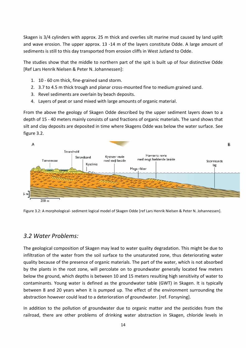
From the above the geology of Skagen Odde described by the upper sediment layers down to a

depth of 15 - 40 meters mainly consists of sand fractions of organic materials. The sand shows that

silt and clay deposits are deposited in time where Skagens Odde was below the water surface. See

figure 3.2.

Figure 3.2: A morphological- sediment logical model of Skagen Odde [ref Lars Henrik Nielsen & Peter N. Johannessen].

3.2 Water Problems:

The geological composition of Skagen may lead to water quality degradation. This might be due to

infiltration of the water from the soil surface to the unsaturated zone, thus deteriorating water

quality because of the presence of organic materials. The part of the water, which is not absorbed

by the plants in the root zone, will percolate on to groundwater generally located few meters

below the ground, which depths is between 10 and 15 meters resulting high sensitivity of water to

contaminants. Young water is defined as the groundwater table (GWT) in Skagen. It is typically

between 8 and 20 years when it is pumped up. The effect of the environment surrounding the

abstraction however could lead to a deterioration of groundwater. [ref. Forsyning].

In addition to the pollution of groundwater due to organic matter and the pesticides from the

railroad, there are other problems of drinking water abstraction in Skagen, chloride levels in

15

groundwater (as a result of seawater) has in many cases been too high in relation to requirements

for drinking water. It is neither legal, nor economically justifiable, to clean drinking water in

Denmark from chloride, i.e. no chloride cleaning process is achieved in Skagen waterworks.

The problem is most markedly during summer periods; because of dryness the recovery amount

per. unit area is large resulting in too much chlorine in the coastal and deep wells. Consequently

the focus in Skagen at the present is on how deep boreholes are, and how deep sea border are to

be found. Groundwater in Skagen lies on a pillow of salt. A boundary between the fresh water

from percolating rainfall and the salty groundwater is formed. As fresh ground water has a lighter

density than the salty groundwater, it will be as a pillow on top of the salty groundwater, leading

to the formation of a fresh groundwater pocket.

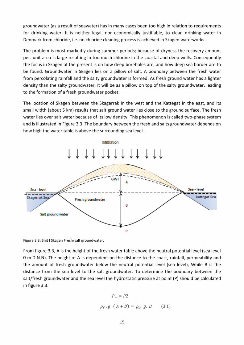
The location of Skagen between the Skagerrak in the west and the Kattegat in the east, and its

small width (about 5 km) results that salt ground water lies close to the ground surface. The fresh

water lies over salt water because of its low density. This phenomenon is called two-phase system

and is illustrated in Figure 3.3. The boundary between the fresh and salts groundwater depends on

how high the water table is above the surrounding sea level.

Figure 3.3: Snit I Skagen Fresh/salt groundwater.

From figure 3.3, A is the height of the fresh water table above the neutral potential level (sea level

0 m.D.N.N). The height of A is dependent on the distance to the coast, rainfall, permeability and

the amount of fresh groundwater below the neutral potential level (sea level), While B is the

distance from the sea level to the salt groundwater. To determine the boundary between the

salt/fresh groundwater and the sea level the hydrostatic pressure at point (P) should be calculated

in figure 3.3:

( ) ( )

16

Where:

P1 Fresh water pressure P2 Salt water pressure

f Freshwater density.

s Saltwater density.

g The gravitational acceleration 9.82 m/s2

A Fresh groundwater height over the sea-level B salt groundwater height over the sea-level

Assumed f = 1000 kg / m3 and s = 1025 kg/m3 in water around Skagen according to (GEUS 2012).

Solving the equation (3.1) to B found B = 40. A, that means if the fresh water is 1 meter under sea-

level the saltwater is 40 m deeper, When the fast pumping starts the reduction to A will reduce B

also resulting saltwater with chloride problems in abstraction of water, however this is not 100%

accurate as the assumption of the boundary between the salt/ fresh ground water level is not

true. See figure 3.4.

Figure 3.4: Snit in Skagen Fresh/salt groundwater during pump

There are three resources for saltwater in the ground water In Skagen. The main is the short

distance to the sea and a long castle in to direction. The second is the groundwater contact with

the dissolved salt from the salted structures and cracks. The third is infiltration of salt from the

surface to the groundwater.

To ensure that extraction water not contains chloride, the GWT kept 2 m above sea level

(m.D.N.N) in this project.

From above we can summarize the problems in drinking water in Skagen to:

1. Low level quality of raw water as the groundwater is near to the earth surface.

17

2. Chloride problems in raw water because of lowering in the groundwater level due to too

much water abstraction.

3. Impacts of abstraction on the surrounding area, which is considered one of the Nature

2000 areas in Denmark.

These problems are very important in limiting the abstraction and supply of water in Skagen. This

project will try to find the best way for resolving the problems of water abstraction and supply.

18

4.1 Drinking Interests area:

Working with water extraction in an area has not only consequences on the nature but it also

affects the environment in underground workings area. This is should be considered in water areas

of interest to be examined.

To protect groundwater in specific area and to ensure good drinking water in the future, a plan

should exist to specify who is responsible for the implementation of various initiatives and when

they should be implemented. This plan determines the necessary efforts to protect groundwater.

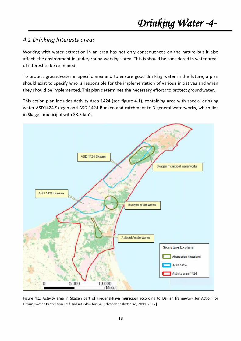
This action plan includes Activity Area 1424 (see figure 4.1), containing area with special drinking

water ASD1424 Skagen and ASD 1424 Bunken and catchment to 3 general waterworks, which lies

in Skagen municipal with 38.5 km2.

Figure 4.1: Activity area in Skagen part of Frederiskhavn municipal according to Danish framework for Action for

Groundwater Protection [ref. Indsatsplan for Grundvandsbeskyttelse, 2011-2012]

Drinking Water -4-

19

From figure 10, ASD 1424 Skagen covers an area of 19 km2 and ASD 1424 deck covers an area of 10

km2. The entire activity area covers an area of 148 km2, where Frederiskhavn Supply A/S has a

great source space in Skagen waterworks and a minor source space in Bunken waterworks.

Land use is predominantly natural and dunes. There are less agricultural areas within ASD and

catchments. There are very few houses in the ASD and catchments. The largest cities in activity

area are Skagen and Aalbaek.

Table 4.1 shows the distribution of the area used in ASD and catchments. Where in the ASD 1424

Skagen and ASD 1424, the deck is natural - and woodland is respectively 88 % and 62% [ref.

Indsatsplan for Grundvandsbeskyttelse, 2011-2012].

Table 4.1: Area used in ASD and catchment [ref. Indsatsplan for Grundvandsbeskyttelse, 2011-2012]

ASD/catchment

Tota

l (km

2)

Ho

use

s (%

)

Agr

icu

ltu

re (

%)

Fore

st (

%)

Nat

ura

l are

as (

%)

Stre

ams

and

la

kes

(%)

Min

ing

Are

as (

%)

Un

rate

d (

%)

ASD 1424 Skagen 19.0 0.1 8.4 21.4 65.8 0.8 0 3.4

ASD 1424 Bunken 10.2 0.3 34.7 6.9 55.0 1.0 0 2.1

Skagen waterworks 6.5 0.1 6.2 73.4 11.9 0.2 0 8.2

Bunk waterworks 3.7 0.0 9.6 57.7 27.1 0.0 0 5.7

Aalbaek waterworks 1.9 0.3 12.7 68.1 12.8 0.2 0 5.9

4.2 Skagen water abstraction:

Skagen supplies drink water from groundwater resource, located in the center of the Skagen

dunes. The field has 32 wells, which are established between 1967 and 2006. All bringers’

condition is good and is equipped with SCADA systems (Supervisory Control and monitoring) (se

figure 4.2), Where the catchments covered about 650 hectares (6.5 km2) and forest / dunes, 74%.

Natural areas account for 12% while agriculture accounts for just 6%.

20

Figure 4.2: Overview of water wells and location of Skagen Waterworks [ref. Indsatsplan for Grundvandsbeskyttelse,

2011-2012].

In all fields areas of best water quality would be found in 10-15 meters below ground type D

(Greatly reduced groundwater with methane). Groundwater aquifer contains natural substances

as iron, organic matter (NVOC) and gases. The average nitrate leaching from agricultural land in

the OSD 1424 Skagen and OSD 1424 are respectively 9 mg / l and 17 mg / l.

4.3 Raw Water Quality:

In Denmark the pumped water from the natural aquifers requires very little treatment at the

waterworks. The sand layers with scattered deposits of peat, no protective clay layer, as well as to

the low-performance of lower part of the aquifer as it consists of silt result to bad raw water

quality and requires water treatment. Table 4.2 show the substances would be found in the water

pumped out from Skagen and the numbers of the wells they contain. The substances are exceeded

in relation to the statutory limits.

21

Table 4.2: The number of wells that exceed the displayed parameters [ref .GEUS 2012a]

Parameter Number of wells

PH 7

Ammonium 32

Chloride 4

Fluoride 3

Iron 32

Potassium 3

Manganese 32

Sodium 2

Nitrate 0

Nitrite 0

Phosphorus (P total) 32

Sulphate 0

Pesticides 0

There are many substances found in all abstractions wells, and the limit measured interval value of these substances shown in table 4.3. Table 4.3: Measured parameters according to the limits [ref GUES .2012a]

Parameter Contents (mg/l) Limit value (mg/l)

Ammonium 0.85 – 6.5 0.05

Iron 6 -16 0.1

Manganese 0.11 – 0.21 0.02

Phosphorus (P total) 0.21 – 0.91 0.15

The raw water must therefore be treated from many substances in Skagen waterworks to reduce

the amount of the over contents parameters. This is a very costly process, and uses a lot of water

to make the water pure enough. This process must be avoided or limited in usage. From 2013

Frederiskhavn municipality planned to supply water (about 950000 m3/ yr.) from Tolne

waterworks, by pipes, keeping Skagen waterworks to continue extracting water. This will roughly

supply half of the recovery needs of the 32 wells. At the same time Bunk waterworks will be

closed. This project will try to determine a good and stable water quality in the aquifers by finding

a recovery strategy which avoids dragging pesticides from the surface down to aquifer. It also

prevents the preferred salt-containing water flowing from the lower part of aquifer into the

portion of the aquifer used for drinking water.

4.4 Water consumption

Skagen consumption of water in 2012 is approximately 1.424.882 m3/ yr. [ref. GEUS. 2012b]. It is expected that the consumption of water for 2019 is 1.724.002 m3/yr. according to [ref. Frederikshavn Kommune, 2012a]. House holding, tourist and factories are the major consumers of the water In Skagen.

22

The number of population in Skagen in 2012 is 8.515 persons. In 2005 calculation of the consumption of water was 131 l/ pr. day as an average. The consumption of water is therefore 407.144 m3/ yr. in Skagen on 2012. Skagen as mention before is an attraction area, where many tourists visit it around the day and part of them overnight in Skagen. This will lead to various consumption of water, an overnighting tourist will consume of about 120 l/pr. d, while for tourist spending only the day will be only is 60 l/ pr. d. This result consumption of water is to be 64.336 m3/yr. and 54.000 m3/ yr. respectively. Fishers market constitutes a big part of the economy of Skagen and need a lot of quantity of water, it consume about 899.401 m3/ yr. of the Skagen consumption. The distribution of the percent of consumption water in Skagen for the three factors as mention above is shown in figure 4.3. [ref. Demarks statistic, 2012]

Figure 4.3: The consumption water distribution in Skagen 2012 with total consumption 1.424.882 m

3/yr.

The water consumption is not constant around the year. It is variable from month to another and it is also variable in the single day from daylight to night. The maximum consumption on the day is found to be between 8-10 o’clock am. And 8 – 10 o’clock pm. [ref. Life winter, 2011]. The tourist season in the Skagen starts on summer from May to August. The consumption of water is increased in these months as shown in figure 4.4.

Figure 4.4: The yearly variation of Skagen water consumption in 2012 according to Skagen waterworks 2.

0250005000075000

100000125000150000175000200000

Wat

er

con

sum

pti

on

[m

3 ]

Month

23

5.1 The Formulation and Definition of Problems:

The formulation of problem solution and analyses in this project is:

How to improve and secure the future water supply of Skagen best, taking into consideration all

the circumstances surrounding the nature and environment, providing the most appropriate

economic solutions.

It is wished to ensure water abstraction and supply to Skagen in 20 - 30 years. To achieve this,

problems of water pollution must be taken in consideration., As previously mentioned in chapter

(water problems) It is important to have a clear vision about the amount of the water used and

expected to be used in the future before starting the analyses finding the way to improve the

water quality and water supply,. The first priority to be accounted is the quality of water,

economic viability of the project, and the protection of nature reserves.

5.2 Suggested solution:

1. Reducing the extraction of the water.

2. Closed wells have chloride constriction.

3. Impact of climate change

Problems -5-

24

Water extraction affects aquifers. The effect of current abstraction will be determined in this

project in two models: one/two dimensional mathematical model and three dimensional

numerical groundwater modeling (GMS-model). To establish these models only the unaffected

ground potential will be calculated. Ground potential will be without water extraction (the

affected groundwater levels simulated a water equal to the force of the current abstraction).

Calculation the lowering of the groundwater will yield water extraction. This is done to make a

validation of groundwater model by comparison with the current water level from GEUS. Based on

this, it is possible to validate groundwater model and thereby come up with a solution for the

future water abstraction in Skagen dune plantation.

6.1 Mathematical Model:

To determine the groundwater potential, which give the general view for the drawdown in groundwater level, a model in MATLAB program was built. The model covers an area of about (4, 5 * 10) km from Skagen. It is starting from the north part of habitats region to the middle part of Skagen city, and to the beach from the west and east part as shown in figure 6.1.

Figure 6.1: The calculation region to the mathematical model.

The groundwater model in MATLAB consists of a mesh from 4500 cells with 50 * 50 m size in a matric principle. Every calculation points represent the calculate point in the real life. The point would be choice to sufficient point to give clear and good results to the flow plot curves with minimum filed mistake. A several assumption need to occur in this model, one homogenous, isotropy layer, and isolated from the north and south with infinity extent. The input data in the model, determined in the annex B are:

Hydraulics conductivity (K) is 9.9 . 10-5 m/s.

Transitivity (T) is 8.8 . 10-4 m2/s.

Groundwater Model -6-

25

Aquifer coefficient (S) is 0.0329.

Net precipitation (Np) is 265 mm/ yr.

The equilibrium time (t) is 9 month. These input data would be used to determine the groundwater table and the drawdown in the groundwater level by using general differential equation (Laplace’s equation) to describe the flow in aquifer [ref. K.Schaarup -Jensen, 1993].:

( )

( )

( )

( )

( )

Where: U(x) The distance from the impermeable layer to the groundwater table as a function of( x) U Infiltration in the top of the reservoir. w Infiltration in bottom of reservoir. Sy Aquifer coefficient. T Transmissivity t Time k The conductivity hydraulic

After shortening Laplace´s equation to 1D as explained on the annex B.4 and insert the input data in, the unaffected groundwater table to Skagen Odde would be determine in 3D and plan figures as shown in figure 6.2 & 6.3 respectively.

Figure 6.2: The unaffected groundwater table 3D to Skagen Odde, which x & y are the coordinated points and z is the

elevation in meter

26

Figure 6.3: The unaffected groundwater table plan to Skagen Odde, which x & y are the coordinated points in meter.

The unaffected groundwater table (UGWT) found from figure 14 to be about 6.10 m over the sea

level (m.D.N.N) on the boundary of the Nature 2000 region near DGU wells no. 4.264. To insure

realism of the calculation, the value of the UGWT must be compared with the measured data from

GEUS 2012. The measured data from GUES for affected GWT is about 6.33 (m.D.N.N), thus only a

minimum difference between the calculation data and measured data is noticed.

Although the measured data is in the high level for affected GWT, it is still acceptable due to the

lack of unaffected GW measured data at the same time the level is not important if the drawdown

for the these two data matched together after extraction water as it will be shown later.

The good matched data near Nature 2000 gives a high GWT value in the Skagen area. The model

would be calibrated with these data and gives hydraulic conductivity equal to 9.9. 10-5 m/s

responses to medium sand soil (9×10-7 - 5×10-4 m/s).

The difference in the results could be related to many reasons. The assumption of the infinity

extent and isolated edges are not really true because the area would be affected by the

streamwater as well as the sea around it. Additionally there was mistake in the reading to the

measured data from GEUS side. The model neglected the topographic changes of the area. All of

the above mentioned factors lead to the variation in the results between the measured data

(GEUS) and calculation data (model), however, this model can still be relied upon in future

accounts.

27

The model show that the water level is near the ground surface in the north part of nature 2000

(about 1 - 2 m under the ground surface) and would be lower in the direction to the Skagen, in

other word there is a problem of the high groundwater table in the north part of the Nature 2000

before the beginning of water extraction.

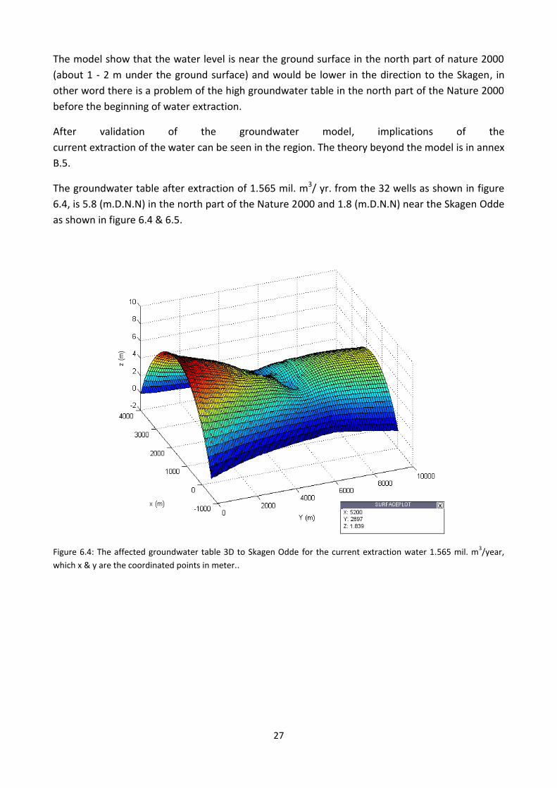
After validation of the groundwater model, implications of the

current extraction of the water can be seen in the region. The theory beyond the model is in annex

B.5.

The groundwater table after extraction of 1.565 mil. m3/ yr. from the 32 wells as shown in figure

6.4, is 5.8 (m.D.N.N) in the north part of the Nature 2000 and 1.8 (m.D.N.N) near the Skagen Odde

as shown in figure 6.4 & 6.5.

Figure 6.4: The affected groundwater table 3D to Skagen Odde for the current extraction water 1.565 mil. m3/year,

which x & y are the coordinated points in meter..

28

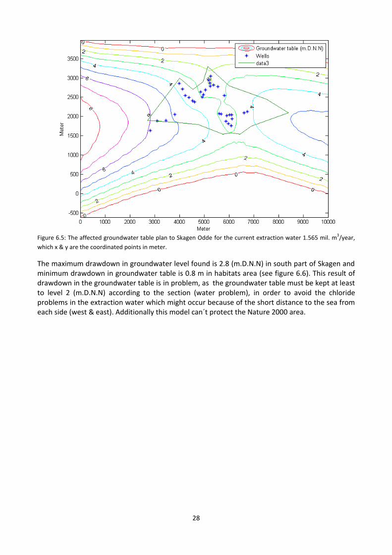
Figure 6.5: The affected groundwater table plan to Skagen Odde for the current extraction water 1.565 mil. m

3/year,

which x & y are the coordinated points in meter.

The maximum drawdown in groundwater level found is 2.8 (m.D.N.N) in south part of Skagen and minimum drawdown in groundwater table is 0.8 m in habitats area (see figure 6.6). This result of drawdown in the groundwater table is in problem, as the groundwater table must be kept at least to level 2 (m.D.N.N) according to the section (water problem), in order to avoid the chloride problems in the extraction water which might occur because of the short distance to the sea from each side (west & east). Additionally this model can´t protect the Nature 2000 area.

29

Figure 6.6: The drawdown in groundwater level for the current extraction water 1.565 mil. m

3/yr.

From another hand the drawdown is large in the Nature 2000 area, which is located in the left side of the boundary lines (green line) in figure 6.6. This drawdown cause’s damage in the area, on the other hand closing the wells in Nature 2000 area will cause flood in the area. The drawdown in the groundwater level is unstable; it depends on the time (seasons) and the place. As the stream flow is dynamic and depends on the extraction water amount, ways to downgrade must be found. To reduce the drawdown in the groundwater level, there are many solutions which would be suggested to discuss in next section.

6.1.1 The Solution:

This section will focus on the ways to improve the water quality in Skagen, and protect Nature 2000 area from being damaged.) It will be discussed in details. The principle of the first solution is based on reduction of the drawdown groundwater to the suitable level, which will avoid the damage in the Nature 2000 area avoiding extraction salty water at the same time. Alternative solution will be to use the sea water instead of the groundwater as a source of drinking water.

6.1.1.1 The Change in the water extraction volume:

Reduction of the drawdown in groundwater as a way to get good quality drink water and keeping the nature 2000 area away from being damaged, the following is suggested:

- Change the extraction water to different amount to 120%, 80%, and 50% from the current extraction water in the area which estimates to 1.568 mil. m3/s [ref. data].

30

- Close the wells which have chlorides problem.

Scenario 1 : In this scenario the suggested solution will be extracting 120% from the current extraction (i.e. about 1.878 mil. m3/yr.). The increase in the extraction amount would be divided equally to all the 32 wells as shown in table 6.1. Table 6.1: The current and suggested extraction amount of water.

DGU. Wells no.

Current case (m3/yr.)

Scenario 1 (m3/yr.)

Scenario 2 (m3/yr.)

Scenario 3 (m3/yr.)

Scenario 4 (m3/yr.)

1.172 49557 59468,4 39645,6 24778,5 49557

1.174 64770 77724 51816 32385 64770

1.193 69619 83542,8 55695,2 34809,5 0

1.194 49331 59197,2 39464,8 24665,5 0

1.195 55371 66445,2 44296,8 27685,5 0

1.197 54618 65541,6 43694,4 27309 54618

1.198 74611 89533,2 59688,8 37305,5 74611

1.248 11832 14198,4 9465,6 5916 11832

1.249 45325 54390 36260 22662,5 45325

1.250 60446 72535,2 48356,8 30223 60446

1.252 53264 63916,8 42611,2 26632 53264

1.253 32389 38866,8 25911,2 16194,5 32389

1.254 68056 81667,2 54444,8 34028 68056

1.267 54584 65500,8 43667,2 27292 54584

1.268 43246 51895,2 34596,8 21623 43246

1.269 17060 20472 13648 8530 17060

1.270 67099 80518,8 53679,2 33549,5 67099

1.271 35535 42642 28428 17767,5 35535

1.272 70589 84706,8 56471,2 35294,5 70589

1.283 32412 38894,4 25929,6 16206 32412

1.284 60857 73028,4 48685,6 30428,5 60857

1.380 53075 63690 42460 26537,5 53075

1.522 10685 12822 8548 5342,5 10685

1.523 51702 62042,4 41361,6 25851 51702

1.524 63705 76446 50964 31852,5 0

1.525 48061 57673,2 38448,8 24030,5 48061

1.526 49658 59589,6 39726,4 24829 49658

1.527 62012 74414,4 49609,6 31006 62012

4.261 24540 29448 19632 12270 24540

4.262 60181 72217,2 48144,8 30090,5 60181

4.263 42234 50680,8 33787,2 21117 42234

4.264 28596 34315,2 22876,8 14298 28596

Sum 1565020 1878024 1252016 782510 1326994

31

Figure 6.7: The drawdown in groundwater level for 120% of the current extraction water.

The drawdown would be increased in Nature 2000 area to be 0.9 m and reduces gradually to the south direction, during this event the groundwater level will varies from 5.2 – 1.472 (m.D.N.N) from Nature 2000 area to Skagen area respectively (see figure 6.7 & 6.8). This solution results in chlorides problems and cannot protect the Nature 2000 area.

Figure 6.8: The affected groundwater table 3D to Skagen Odde for the 120% of the current extraction water, which x &

y are the coordinated points and z is the elevation in meter.

32

.

Scenario 2: In this scenario the solution suggested is extracting 80% from the current extraction (i.e. about 1.252 mil. m3/yr.). The decrease in the extraction amount would be divided equally to all the 32 wells as shown in table 6.1. The drawdown would be decrease in Nature 2000 area to be 0.6 m and 2.2 m in Skagen. And it is reduce gradually to south direction, during this event the groundwater level will varies from 6.5 – 2.489 (m.D.N.N) from Nature 2000 area to Skagen area respectively (see figure 6.9 & 6.10). This solution is in the critical limit of the chlorides problems; however, it doesn’t protect Nature 2000 area yet.




33

Scenario 3: In this scenario the solution suggested is to extract 50% from the current extraction (i.e. about 0.782 mil. m3/yr.). The decrease in the extraction amount would be divided equally to all the 32 wells as shown in table 6.1. The drawdown would be decreased in Nature 2000 area to be 0.4 m and 1.3 m in Skagen. And it is reduce gradually to south direction, during this the groundwater level would varies from 7 – 3.251 (m.D.N.N) from Nature 2000 area to Skagen area respectively (see figure 6.11 & 6.12). This solution is within the safety side from the chlorides problems and it protects Nature 2000 area.




34

Scenario 4 In this scenario the solution suggested is to close all the wells, which have chloride constriction more than 250 mg/l. The extracting of the remaining wells would be the same like current extraction as shown in table 6.1. The drawdown would be in Nature 2000 area to 0.7 m and 2.5 m in Skagen. And it is reduce gradually to south direction, While the groundwater level would varies from 5.5 – 2.214 (m.D.N.N) from Nature 2000 area to Skagen area respectively (see figure 6.13 & 6.14). This solution is in the critical limit of the chlorides problems; however, it does not protect the Nature 2000.

Figure 6.13: The affected groundwater table 3D to Skagen Odder for the current extraction water with closing chloride

wells, which x & y are the coordinated points and z is the elevation in meter.

Figure 6.14: The drawdown in groundwater level for the current extraction water with closing chloride wells.

35

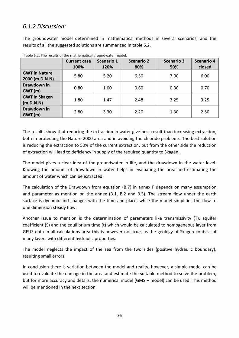
6.1.2 Discussion:

The groundwater model determined in mathematical methods in several scenarios, and the

results of all the suggested solutions are summarized in table 6.2.

Table 6.2: The results of the mathematical groundwater model.

Current case 100%

Scenario 1 120%

Scenario 2 80%

Scenario 3 50%

Scenario 4 closed

GWT in Nature 2000 (m.D.N.N)

5.80 5.20 6.50 7.00 6.00

Drawdown in GWT (m)

0.80 1.00 0.60 0.30 0.70

GWT in Skagen (m.D.N.N)

1.80 1.47 2.48 3.25 3.25

Drawdown in GWT (m)

2.80 3.30 2.20 1.30 2.50

The results show that reducing the extraction in water give best result than increasing extraction,

both in protecting the Nature 2000 area and in avoiding the chloride problems. The best solution

is reducing the extraction to 50% of the current extraction, but from the other side the reduction

of extraction will lead to deficiency in supply of the required quantity to Skagen.

The model gives a clear idea of the groundwater in life, and the drawdown in the water level.

Knowing the amount of drawdown in water helps in evaluating the area and estimating the

amount of water which can be extracted.

The calculation of the Drawdown from equation (B.7) in annex F depends on many assumption

and parameter as mention on the annex (B.1, B.2 and B.3). The stream flow under the earth

surface is dynamic and changes with the time and place, while the model simplifies the flow to

one dimension steady flow.

Another issue to mention is the determination of parameters like transmissivity (T), aquifer

coefficient (S) and the equilibrium time (t) which would be calculated to homogeneous layer from

GEUS data in all calculations area this is however not true, as the geology of Skagen contsist of

many layers with different hydraulic properties.

The model neglects the impact of the sea from the two sides (positive hydraulic boundary),

resulting small errors.

In conclusion there is variation between the model and reality; however, a simple model can be

used to evaluate the damage in the area and estimate the suitable method to solve the problem,

but for more accuracy and details, the numerical model (GMS – model) can be used. This method

will be mentioned in the next section.

36

6.2 (3D) Numerical Model (GMS – model):

The main purpose of this chapter is to describe the set-up of groundwater of Skagen model, and how the parameters are calibrated and validated. A laboratory experiment will also be described as it is conducted to investigate, validate and calibrate the groundwater model. For a better understanding of the program and its options a short introduction to GMS 8.3, which is used to build the Skagen groundwater´s model, is presented.

6.2.1 GMS 8.3 model:

Due to the limited knowledge of the geological conditions, different flow directions of the groundwater are possible. Three geological models were therefore built in the software GMS 8.3 by Aquaveo(Groundwater Modeling System version 8.3), which is software for numerical groundwater modeling. This is based upon finite difference solution of the combined continuity equation and Darcy equation in three dimensions given as:

( )

Where

Kx The hydraulic conductivity x-direction (m/s). Ky The hydraulic conductivity y-direction (m/s). Kz The hydraulic conductivity z-direction (m/s). H The total head (m). R Sink/ source term (s-1) Ss The specific storage (m-1). t The time (s).

The Skagen models can be directly transformed from large scale to small scale in the lab. A small scale experiment has been executed to calibrate and validate GMS model of Skagen as described in the next section.

6.2.2 Calibration of the GMS – Model:

6.2.2.1 Lab experiment:

The lab experiment consists of a basin (L1500 x B400 x H600) mm as shown in figure 6.15. Filled

with two different sand layers 200 mm. The bottom layer is a fin sand texture layer with hydraulic

conductivity (K) = 1.8. 10-4 (m/s) [see annex C.1], and the top layer is a medium sand texture layer

with K = 2.38. 10-4 (m/s) [see annex C.1]. After 880 mm from the left side and on the middle from

the front side two water pumps were set, this pumps out different water quantity.

37

Figure

6.15: The basin of the lab experiment.

The water in the system would come from the left and right edges of the basin representing

Skagerrak and Kattegat Sea respectively. The edges are separated by filters. In the system the right

level equals the left level which is 350 mm. after pumping the total water; head would be

measured from 6 different points, 60 mm from the front side, as shown in the figure 6.16.

Figure 6.16: The total measured head profile of the lab experiment when the pumping water P3 = 0.003298 (l/s).

The figure gives an image of the groundwater table of the basin when the abstraction of the water

stat out of the system. The lowest point is the nearest point to the pumping point.

The model would be simulated in GMS 8.3 program. A simple model with a grid from 10 x 10 x 10

mm in 3D would be applied. The GMS groundwater model of the basin and the calibration of the

model can be seen in figure 6.17 & 6.18 respectively.

pump out with Q

400 mm

350

350 mm

25 230 230 260 360 365 30

1500 mm

200

200

280

300

320

340

360

380

0 200 400 600 800 1000 1200 1400 1600

Tota

l he

ad [

mm

]

Distance [mm]

P3

38

Figure 6.17: The total GMS head profile in pump section of the lab experiment when the pumping water P3 =

0.003298 (l/s).

Figure 6.18: The result of the calibration of the lab experiment when the pumping water P3 = 0.003298 (l/s).

The differences in the readings of the total head to several points are showed in figure 6.18. The

difference between the GMS and the measured data is (-1 to 6) mm. this might be due to the fact

that the filter in the edges of the basin were not 100% sealed or it could be related to errors in

measurements.. However a difference op to 6 mm should be acceptable. The lab experiment will

be completed with pumping different water quantity in the annex C.2.

280

300

320

340

360

380

0 200 400 600 800 1000 1200 1400 1600

Tota

l he

ad [

mm

]

Distance [mm]

P3

39

6.2.3 Skagen model setup

The GMS model of Skagen is based on the MODFLOW as calculate in GMS model achieved from NIRAS A/S, and Hedeselskabet in collaboration with north Jutland rapport. It covers all Skagen Odde towns. The GMS – model is chosen because it is well suited for handling the coupling between the conceptual model and numerical model, including model data in GIS format (boundary conditions, geological, hydraulic conductivities and zones, wells, infiltration mm.). The model consists of number of boxes in a mesh system (200 x 200) m, where a finite difference solution to the governing equation 6.2 could be set up for each box, after inset known area´s boundary conditions, geology information and several input data resulting in N finite difference solutions for N unknown heads, which were solved in a numerical scheme to a converging solution. The model covered 230 Km2 that means 5750 cells in every 5 layers. The mesh would be finer around the Skagen Waterwork II area to give good results. See figure 6.19 & 6.20.

Figure 6.19: The hydraulic definition of the model [ref. Nordjyllands Amt] for Skagen Odde

The geology of the model would be developed by DEM of north Jutland and GEUS data, which NIRAS A/S selected the model consisting of 5 layers [ref. NIRAS Notat]: (se figure 6.19)

Wind Deposited sand with peat layer (layer 1), approx. 4 m.

Beach sand deposits (layer 2), approx. 2.5 m.

Revel and rendering deposits (layer 3), approx. 4 m.

Storm Sand layer (layer 4), mighty ranging from below the limit of layer 3 to the surface of layer 5.

40

Figure 6.20: SW-NE cross-section profile (section 1) and NW-SE oriented cross-section (section 2) through Skagen

Odde, showing tremendous importance of the 5 layers that are part of DEM geological model [ref. NIRAS Notat]

The boundary conditions of the model is assumed at the outflow zone modeled by only putting

pressure boundary condition in layer 1 or layer 2, and the saltwater border is variable from level –

9 m in the west coast from Skagen dune plantation and to level – 2 m from the east as shown in

figure 6.21, the pressure along the coastline in all layers coastline to the model are constant and

equal to zero meter. [ref. NIRAS Notat].

Figure 6.21: The conceptual model of the of the water exchange between the aquifer and the sea [ref. NIRAS Notat].

41

The hydraulics conductivity of the model distributed to 3 hydraulic units:

1. Wind Deposited sand with peat layer (layer 1), Beach sand deposits (layer 2), Revle and

rendering deposits (layer 3).

2. Storm Sand layer (layer 4).

3. At the bottom (layers 5) marine silt with a low hydraulic conductivity of 5.10-5 m / s.

Data for groundwater table, bearings and runoff from Knasborg Å is used to calibrate the model,

for describing the situation at Skagen Waterworks 2 and its region, and good adaptation of

pressure levels around the well field in Skagen dune plantation and south of that. The best fit to

hydraulic conductivity by using the inverse calibration method, is found in table 6.3, with a mean

error (ME) of 0.02 m, mean absolute error (MAE) of 0.46 m and Root-mean-square error (RMS) of

0.54 m.

Table 6.3: The calibration hydraulic conductivity ref. [ref. NIRAS Notat]

K (m/s)

Unit 1 2.74 . 10-4

Unit 2 9.11 . 10-5

Unit 3 Not calibra (5 .10-5)

Horizontal anisotropy factor 5.5

Assessments can be supported by the model scenarios and future recovery strategies can thus be

tested and evaluated on model results.

All streams in the investigation area are modeled as drain and not as rivers (which the water flow

out of the groundwater aquifer and not in it), because moldering with drains give a limit leakage of

water streams, at the same time the model based on steady state conditions, yielding a small

error. on the other hand the flux, (when using of rivers) depends on differece of pressure

between the groundwater potential and water levels in rivers , the streams conductance and not

on the reality water in those basin, resulting error in water balance when rivers is used. The data

are from Knasborg Å for 20 point measured for the period April 1987 to December 1988. The

average water flow from the hydrological catchment area is calculated to 683 l/s with a total area

of 56.5 km2 of the topographic basin corresponds to a runoff of 381 mm. [ref. NIRAS Notat].

There are many parameters which are difficult to estimate and describe in the MODFLOW GMS –

model, like water flow in unsaturation area, water flow on the surface (except streams), coupling

between the groundwater table and the actual evapotranspiration, and the influence of the

density of flow. In this model there is state flow model without dynamic coupling between the

saturation zone and unsaturation, which lead to the groundwater recharge variable with place.

The net precipitation (Np) in this model is 265 mm/ yr. as shown in annex B.1.

42

6.2.4 Skagen model results:

After applying of all above data and simulation the GMS model the unaffected groundwater in

Skagen is shown in figure 6.22.

Figure 6.22: The unaffected groundwater table to Skagen Odder on the first layer in GMS model, where the gray area

represents the dry cells and the yellow circle represents the 32 wells.

From figure 6.22 on can notes the Nature 2000 area is located in the area which the head near

DGU wells no. 4.264 approximately between (8.78) m, while the south of Skagen the head is

between (7.50) m (near DGU well no. 1.193). The side view of the model is clear in figure 6.23.

Figure 6.23: The unaffected groundwater table to Skagen Odder on the side view of GMS model, where the yellow

circle represents the 32 wells.

43

The groundwater potential is falling towards north with the logically measured data from GEUS. the GWT in the Nature 2000 area is 0.62 m under earth surface (ES) (where level of surface earth in well no. 4.264 is 9.4 m.D.N.N), this is important to extraction of water to avoid the flood in this area. The extraction water from this level has risk of pollution with the chemical substances which can come from the human use. The GWT in Skagen Odde is in the same level of earth surface (where level of surface earth in well no. 1.193 is 7.5 m.D.N.N), having the same problem of water extraction as there is risk of pollution with remnants of the agricultural and industrial rights. The distribution of the groundwater potential from the west to the east is shown in figure 6.24, which the side view is in the DGU well number 4.264.

Figure 6.24: The unaffected groundwater table to Skagen Odder on the front view of GMS model in the DGU well no.

4.264, where the left side Skagerrak coastline and the right side is the Kattegat coastline.

The view gives a good description for the groundwater in the nature 2000 area, where the head is zero in both sides (coastlines side) and increases towards the inside. In the other side of the model specifically at the area in Skagen Odde, the side view of the DGU well number 1.193 is showed (see figure 6.25).

44

Figure 6.25: The unaffected groundwater table to Skagen Odder on the front view of GMS model in the DGU well no.

1.193, where the left side Skagerrak coastline and the right side is the Kattegat coastline.

The groundwater potential views as shown in figure 6.26, after the current extraction of the water

1.565 mil. m3/year (see table 6.1).

Figure 6.26: The affected groundwater table to Skagen Odder on the first layer in GMS model and for current

extraction water 1.565 mil. m3/year, where the gray area represents the dry cells, and the blue circle represents the

32 wells.

From figure 6.26 there are many dry areas (gray cells) in the Skagen waterwork 2 areas. The water

head would be increased gradually toward south to Nature 2000. The groundwater table (GWT) in

Nature 2000 area near DGU well no. 4.264 is approximately (6.96) (m.D.N.N) while in Skagen Odde

area near DGU well no. 1.193 is (4.75) (m.D.N.N). In section (water problems) the level of

groundwater will be limited to 2 (m.D.N.N) to avoid the chloride problems, and in the same time

45

the groundwater table must be kept in a certain level to avoid the damage in the Nature 2000.

From the affected groundwater table data in figure 6.26 the GWT after extraction the current

water amount is 2.44 m under earth surface in the Nature 2000 and 2.75 m in the Skagen Odde,

that is too much to the small plants to get water, as the moisture zone is not in the roots zone for

small plants with shallow roots leading to the damage in the Nature 2000. There are many

suggested solution as mentioned early in (water problems section) to avoid this problem and

keeping the area in the safety side from the flood caused by the stopped extraction of water or

decreasing it.

6.2.5 Suggested Solutions:

The same principle in mathematical model would be suggested and same solution will be

discussed. This section focuses in modeled the different extraction water as shown in table 6.1 for

all the 32 wells in the interesting project area.

Scenario 1 Start with modeled 120 % of the current extraction water response to 1.878 mil. m3/s, and the

results of the groundwater table 6.1 is shown in figure 6.27.

Figure 6.27: The affected groundwater table to Skagen Odder on the first layer in GMS model and for 120% of the

current extraction water 1.878 mil. m3/year, where the gray area represents the dry cells, and the blue circle

represents the 32 wells.

The figure shows the groundwater table in Nature 2000 near DGU well no. 4.264 is (6.57) m.D.N.N,

while in the Skagen Odde near DGU well no. 1.193 is approximately (4.13) mD.N.N. This suggest

scenario which gives problem in protecting the Nature 2000 from drought and small plants shrubs

death. The GWT is 3.83 m under the earth surface, for a solution to be in the safety side from

chloride problems, the GWT should be more than 2 meter over the sea level.

46

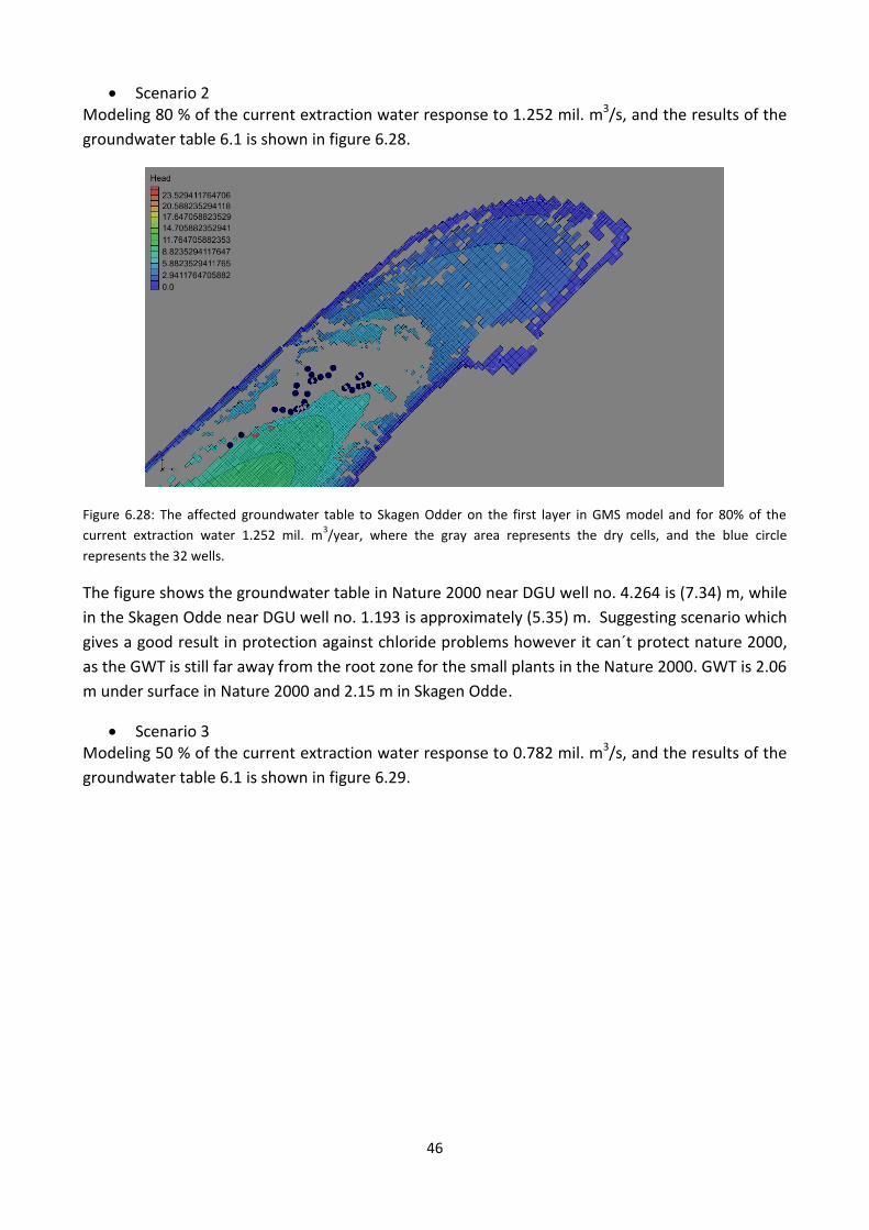
Scenario 2 Modeling 80 % of the current extraction water response to 1.252 mil. m3/s, and the results of the

groundwater table 6.1 is shown in figure 6.28.


current extraction water 1.252 mil. m3/year, where the gray area represents the dry cells, and the blue circle


The figure shows the groundwater table in Nature 2000 near DGU well no. 4.264 is (7.34) m, while

in the Skagen Odde near DGU well no. 1.193 is approximately (5.35) m. Suggesting scenario which

gives a good result in protection against chloride problems however it can´t protect nature 2000,

as the GWT is still far away from the root zone for the small plants in the Nature 2000. GWT is 2.06

m under surface in Nature 2000 and 2.15 m in Skagen Odde.

Scenario 3 Modeling 50 % of the current extraction water response to 0.782 mil. m3/s, and the results of the

groundwater table 6.1 is shown in figure 6.29.

47


current extraction water 0.782 mil. m3/year, where the gray area represents the dry cells, and the red circle



in the Skagen Odde near DGU well no. 1.193 is approximately (6.25) m. suggesting a scenario

which gives a good result to protect water against chloride problems and protect nature 2000, the

GWT is 1.54 m and 1.25 m under surface in Nature 2000 and Skagen Odder respectively.

Scenario 4 This scenario suggests closing all the wells, which have chloride constriction more than 250 mg/l.

The extracting of the remaining wells would be the same as current extraction response to 1.326

mil. m3/s as shown in table 6.1, and the results of the groundwater table is shown in figure 6.30.

Figure 6.30: The affected groundwater table to Skagen Odder on the first layer in GMS model and for the current

extraction water with closing chloride wells, where the gray area represents the dry cells, and the blue circle


48


in the Skagen Odde near DGU well no. 1.193 is approximately (5.82) m. this suggest a scenario

which gives a good result to protect water against chloride problems ;however it can´t, protect

nature 2000.

6.2.6 Discussion:

The results of the GMS modeling to all scenarios are summarized below in table 6.4:

Table 6.4: The results of the numerical groundwater model (GMS).

Unaffected GWT

Current case 100%

Scenario 1 120%

Scenario 2 80%

Scenario 3 50%

Scenario 4 closed


8.78 6.96 6.57 7.34 7.86 7.12


7.50 4.75 4.13 5.35 6.25 5.82

The results of the mathematical modeling to all scenarios are summarized below in table 6.5:

Table 6.5: The results of the mathematical groundwater model.

Unaffected GWT

Current case 100%

Scenario 1 120%

Scenario 2 80%

Scenario 3 50%

Scenario 4 closed


6.10 5.80 5.20 6.50 7.00 6.00


4.90 1.80 1.47 2.48 3.25 3.25

The GMS model explains the differences between all of the suggested solution to improve the

quality water extraction from Skagen, and to suggest which one of them is the best. Decreasing

the extraction to the 50 % of the current extraction is the best for the Nature 2000 area and it is

far away from the saltwater level; however the amount of extraction water is not enough to cover

the usage of the population of Skagen Odde.

The two models (numerical and mathematical)as shown in tables 9 &10 respectively, give the

same result when the solution is reducing the extraction of water to 50%, however the two

models could not get similar value results in all solutions. There is a big variation in the values

between the two models in the solutions. There is 17.7 % deviation in the results in the Nature

2000 and 51% deviation in results in Skagen area.

The GMS model is more accurate and gives more details about the area from geology; it gives

complete details of the hydraulic process in the groundwater in 3D in addition to its simplicity in

usage. The data can easily and quickly be changed. The model still has small error in the

49

calculations caused by the difficulty in giving the exact geological information of the area as well as

the variation in orientation of the place (horizontal versus vertical).

the model assumption of the steady state flow conditions over all model, the water flow out of the

groundwater aquifer and not in, the error in the water balance, caused by flux in the system which

depends on the difference of pressure between the groundwater potential and water levels in

rivers and the streams conductance (not on the reality water in those basin), the estimate of the

evaporation and the really precipitation. All these factors causes’ small errors in the results

compared with the real life model. As NIRAS A/S has calculate to a mean error (ME) of 0.02 m,

mean absolute error (MAE) of 0.46 m and an Root-mean-square (RMS) of 0.54 m for GMS model

[ref. Nordjyllands Amt ]. Therefore, this model can trust on and used in future recovery strategies.

50

7.1 Impact of climate change

The groundwater is one of the elements which consist the water circle in the nature, it consists 30

% of the water in the earth. The water circle in a simple description consist of part of the surface

water which infiltrates into the earth creating groundwater, while another part evaporates to

become rain after many processes. There are therefore many factors affecting the groundwater

amount, the level and water quality. The change in the climate is one of important factor like the

temperature, the wind, the season and the precipitations, which have big impact on the amount

of water infiltration into earth thus affecting the groundwater.

This section focuses on the precipitation as one of the climate factors impacting on the

groundwater. A GMS model would be simulating to show the effect of the change on the amount

of the precipitation on the groundwater table. The model simulating the current extraction of the

water 1.565 mil. m3/year in 3 models. The first simulates with 265 mm/yr., the second with 200

mm/ yr. and the last with 300 mm/yr. as shown in figures 7.1, 7.2 and 7.3 respectively.

Figure 7.1: The affected groundwater table to Skagen Odder on the first layer in GMS model and for current extraction

water 1.565 mil. m3/year and precipitation 265 mm/yr., where the gray area represents the dry cells, and the yellow


Climate -7-

51


water 1.565 mil. m3/year and precipitation 200 mm/yr., where the gray area represents the dry cells, and the red



water 1.565 mil. m3/year and precipitation 300 mm/yr., where the gray area represents the dry cells, and the red


52

The results of all simulating are summarized in the table 7.1 below:

Table 7.1: The results of the numerical groundwater model. For different precipitation.

100% extraction NP =265 mm/yr.

Head (m)


Head (m)


Head (m)

Earth surface(ES) level (m)


6.96 5.48 7.69 9.4


4.75 3.89 5.30 7.5

GWT level under ES in Nature 2000

2.44 4.02 1.81

GWT level under ES in Skagen Odde

2.75 3.61 2.2

Where ES: earth surface

The results show that simulate with 300 mm/ yr. give a good result for protecting the Nature 2000,

and avoiding the chloride problems, while simulate with 200 mm/ yr. causes desertification and

drought problem. This clearly shows the impact of climate on the groundwater, as precipitation is

one of the main resource of the groundwater and explains why there are different levels of

groundwater from one season to another, for instance the high level in the winter due to the low

temperature and heavy raining whereas the low level in summer is related to the high

temperature and less raining.

53

In the last period Skagen Odde has bad quality drinking water problems caused by the excessive

water extraction in Skagen waterworks 2, which has also damage effect on Nature 2000 as located

in the south part of the area of the Skagen waterwork.

These problems are the basic of this project. Two models were used to explain the problem and

find alternative solutions (mathematical model and GMS model). Both models are built on the

theory of the fluctuating of the GWT and the drawdown in the level as a result of water extraction.

The main aim is to find out the suitable amount of water that can be extracted without damaging

the nature.

After several suggested solution the project conclude that decreasing the extraction of water to 50

% from the current extraction 1.565 mil. m3/year is the best solution, however it doesn´t cover

Skagen usage of the water, thus Skagen need an external supply of the drinking water.

There are many suggestions to supply the rest of water, for example: desalination the sea water,

which is expensive because of the need to energy and it, is not friendly to the nature. Another

suggestion is to supply water from the near area as Tolne, this need to establish pipes from Tolne

to Skagen causing this suggestion to be also expensive.

The project shows the difference between the two models. The best, easy and more accurate one

is the GMS model. GMS model gives more details, 3D flow and covered large area with large

depth.

Summary -8-

54

Visit Skagen . URL:http/www.visitskagen .dk / om skagen/ fakta.

Nature 2000, plan 2010- 2015. Natura 2000-plan 2010-2015. Skagens Gren og Skagerrak. Natura 2000-

område nr. 1 Habitatområde H1e.

URL:http://www.naturstyrelsen.dk/NR/rdonlyres/9121021B-0C57-4BB0-BAEC-

B8D59A0FF198/0/001Plan.pdf.

Miljøministeriet – Naturstyrelsen. Miljøcenter Nordjylland.Natur 2000 – område Skagen Gren and

Skagerrak.. URL: http://miljoegis.mim.dk/cbkort?profile=miljoegis-natura2000

Lars Henrik Nielsen & Peter N. Johannessen. Skagen Odde et fuldskala, naturligt laboratorium

Forsyning. URL.:http//http://www.forsyningen.dk/vand/PROJECT/Forsyningen - Vandkvalitet.mht

Indsatsplan for Grundvandsbeskyttelse, 2011-2012. Kortlægningsområde (Skagen vandværk,

Bunken vandværk og Ålbæk vandværk)

GEUS. 2012a. Vandprøver fra Skagen vandværk.

URL.:http/data.geus.dk/jupiterwww/anleag.jsp?anlaegid=70624, 2012. set 22.09.2012

GEUS. 2012b. Vandkredsløb

URL.:http/geus.dk/geusmap/indexjupiter.jsp?imgxy=601+322&imapwidth=1201&imapheight=644, 2012.

set 26.09.2012

Frederikshavn Kommune, 2012a. Tursime redegørelse 2011.

URL.:http//www.fredierkshavn.dk/documents/center_for_udvikling_og_erhverv/turismeredeg.

Frederikshavn Kommune, 2012b. Vandforsyningsplan 2009-20019.

URL.:http//www.fredierkshavn.dk/rodnlyres/64B401C6-AD86-4A1C-A5A6-

CF5183664697/0/vandforsyningsplan20092019.pdf, 2012. set 26.09.2012.

Demarks statistic, 2012. URL.:http//www.statistikbanken.dk.

Life Winther, Jens Jørgen Linde, 2011. Afløbsteknik: ISBN: 978-87-502-1015-3, handbook. polyteknisk

K.Schaarup -Jensen, 1993. k. Schaarup – Jensen. Groundvandstrømning 1993

Data. Projecl data – Ole Ole Munch Johansen

Nordjyllands Amt. Appendiks A: Modeldokumentation for opstilling af grundvandsmodel for

Skagen odde. Modelversion 1 - November 2004.

NIRAS Notat. Skagen vandværk 2 Bilag 4.1 – Justering af grundvandsmodel for Skagen Odde

Bibliography -9-

http://www.naturstyrelsen.dk/NR/rdonlyres/9121021B-0C57-4BB0-BAEC-B8D59A0FF198/0/001Plan.pdf

http://www.naturstyrelsen.dk/NR/rdonlyres/9121021B-0C57-4BB0-BAEC-B8D59A0FF198/0/001Plan.pdf

http://miljoegis.mim.dk/cbkort?profile=miljoegis-natura2000

55

A. The wells data:

The wells´s data, used in groundwater model to Skagen Odde would be shown in the following

table:

Table A.1: The pump well and observation wells due to [ref GEUS, 2012].

DGU no. XUTM (m)

YUTM (m)

Depth (m)

Aim of used Constriction years

4.261 588393.46 6396618.16 19 Water supplied 2005

4.255A 588386.46 6396613.17 10 Pejleboring 2005

4.257C 588414.47 6396570.18 10 Pejleboring 2005

Annex -10-

56

B. Theory of the Groundwater model

This chapter focuses on the theory of calculation of the mathematical model and all the

parameters needed to describe the groundwater model with and without water extraction.

B.1 Net precipitation (Np):

From geology of Skagen there is no surface runoff in or near Skagen, therefor the net-precipitation (infiltration) of Skagen, which used to give the total image of the groundwater model in Skagen equal to the total precipitation minus evaporation.

( ) For the north part of Denmark the average annual mean runoff is 10.1 l/s1 /km 2 corresponding to 300 mm [ref. Afstrømningsforhold i danske vandløb Faglig rapport fra DMU, nr. 340 , Fagdatacenter for hydrometri, Miljø- og Energiministeriet Danmarks Miljøundersøgelser]. And the annual mean rainfall of north part is 675 mm [ref. Life Winther]. From that the evaporation determines:

⁄ The net precipitation of Skagen for the annual mean precipitation 600 mm/year [ref. Life Winther] according to the equation B.1 is:

⁄

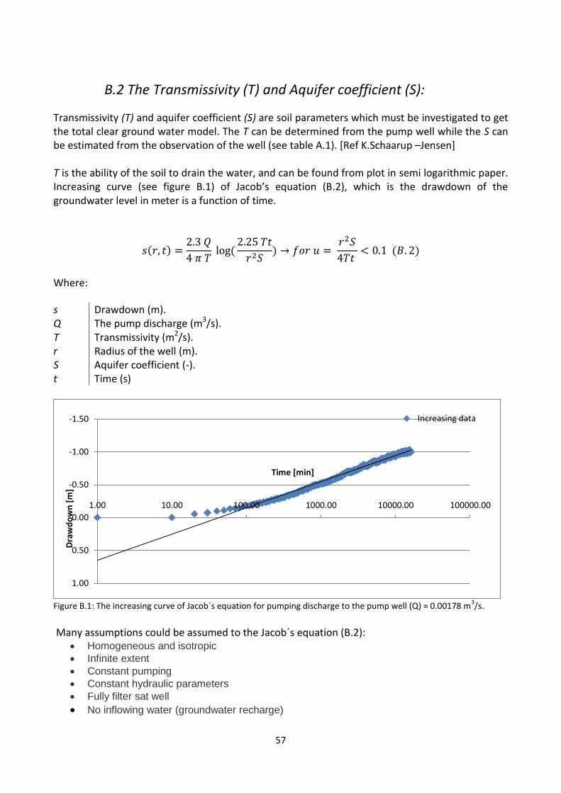
57

B.2 The Transmissivity (T) and Aquifer coefficient (S):

Transmissivity (T) and aquifer coefficient (S) are soil parameters which must be investigated to get the total clear ground water model. The T can be determined from the pump well while the S can be estimated from the observation of the well (see table A.1). [Ref K.Schaarup –Jensen] T is the ability of the soil to drain the water, and can be found from plot in semi logarithmic paper. Increasing curve (see figure B.1) of Jacob’s equation (B.2), which is the drawdown of the groundwater level in meter is a function of time.

( )

(

)

( )

Where:

s Drawdown (m). Q The pump discharge (m3/s). T Transmissivity (m2/s). r Radius of the well (m). S t

Aquifer coefficient (-). Time (s)

Figure B.1: The increasing curve of Jacob´s equation for pumping discharge to the pump well (Q) = 0.00178 m

3/s.

Many assumptions could be assumed to the Jacob´s equation (B.2):

Homogeneous and isotropic

Infinite extent

Constant pumping

Constant hydraulic parameters

Fully filter sat well

No inflowing water (groundwater recharge)

-1.50

-1.00

-0.50

0.00

0.50

1.00

1.00 10.00 100.00 1000.00 10000.00 100000.00

Dra

wd

ow

n [

m]

Time [min]

Increasing data

58

After shortening of Jacob´s equation and plot in semi logarithmic, the equation will be:

From figure B.1 the s = 0, 3666 that is the mean equivalent value of T which is 0.000888 m2/s for Skagen from pump well is 4.261 and pumping discharge = 0.00178 m3/ s. S is the ability of aquifer to store and release water in relation to the aquifer´s total volume. It can be found from plot in semi logarithmic paper from the increasing curve for the observation wells to Jacob´s equation (B.2). At the start when the time t = t0 the drawdown on the water is zero and the S would be found:

S is the two observation wells as shown in figure (B.1), which are in the table below (B.1)

Table B.1: Input data to determine the aquifer coefficient S.

well Time (s) S(-)

DGU nr.4.255A 2436 0.065820

DGU nr.4.257C 87 0.000063

From the table one can notes the big difference in S value which leads to the difference in the distance from the observation well to the pump well. The distances from the observation well to the pump well are 52 m and 8 m for the DGU no. 4.257C and DGU no. 4.255A respectively. In this project the average S = 0.0329 would be used. T and S are unstable values which depend on the hydraulic parameters and activities. It is not easy to determine these values accurately, furthermore Jacob´s equation can´t apply on Skagen, as Skagen has 5 km width and it has boundary with sea from left and right, and this is a contrary to the assumption of the infinity extent.

59

B.3 Determine the equilibrium time (t):

The equilibrium time will be estimated when the drawdown in the groundwater table is in the maximum, and the abstraction of water is in balance with the net precipitation. The balance in system will be represented in the following equation:

( ) Where Np The annual net precipitation (m/ yr.). F The catchment area (m2). Q The abstraction water amount (m3/yr.). The catchment area for one year is 1.565 million m3 and current extraction water amount is 265 mm/yr. precipitation is 5.585 km2 after using equation (B.3). The catchment area for the area of extraction water depends on the time to calculate, causing difficulty in calculation. From the water table and map to Skagen, the catchment areas were found. After drawing the flow lines perpendicular to the pressure lines, one can approximately calculate catchment areas. Different trials of the time (large and small than one year) used to fit to the catchment area equivalents to the area of one year of extraction current water, It would the equilibrium time determined to be equal to 9 month as shown in the table (B.2) below after applied equation (B.3):

Table B.2: The tries equilibrium time.

Time (month) Area (km2)

9 5.234

12 5.584

15 6.011

60

B.4 The unaffected Groundwater Potential:

The aim of determining the unaffected groundwater potential is to give an idea of the water table

level in Skagen before starting the extraction of the water, hereby being able to assess the damage

to the region. The principle of determining the unaffected groundwater potential is based on

Dupuit - Forchheimer equation (B.4), where the free water table depend on the time and the

place. [ref. K.Schaarup -Jensen], as shown in figure (B.2).

Figure B.2: The Principle sketch to determine the unaffected groundwater potential.

( )

( )

( )

( )

( )

Where

U The height over the impermeable layer (m). x The place on x- Axis (m). Y The place on y- Axis (m). w Infiltration under the (m3/yr.). Np Infiltration from percolation (m3/yr.). K Permeability coefficient (m/s). S Aquifer coefficient (-). T Transmissivity (m2/s). t Time of flow (s).

From geology of the place, Skagen has extention in the length according to width in addition to the

slop of water table which is usualy small. The vertical velocity can be neglected leading to the

ability to assume one direction flow of underground water in x- axis. After shortning and

integration, the equation (B.4) and insat boundary condition (the castline have the same pressure

niveau h0=hL ). Thus, the equation (B.5) for calculating the unaffected groundwater levels will be:

( ) √

( ) ( )

This equation would be programed in MATLAB program to determine the unaffected groundwater

potential.

61

B.5 The affected Groundwater Potential:

This section is to show the water table level after starting the extraction water and observes the drawdown in the water level and the changes in the Skagen natur. The principle beyond that is based on the Theis- equation in 2D model[ref. K.Schaarup -Jensen]:

( )

∫

( ) ( )

where:

And the drawdown in water level is:

∑ ( )

∑

( ) ( )

And:

h The pressure level to the affected groundwater table (m). h0 The pressure level to the unaffected groundwater table (m). s The drawdrown in the groundwater level (m). Qb Water extraction (m3/s). W(u) Wellfunction (m). n Number of calculation. T Transmissivity (m2/s).

From above the lowering(drawdown) in the watertable level depends on wellfunction, which can

be solved by infinite series of expansion in MATLAB programme. And it solve to (u < 0.1) for stable

calculation. The lowering would be calculated for 32 wells ,which is located close to each other,

that lead to overlap lowering results. To avoid this problem, the lowering in water level would be

calculated to every well in every piont in matrix system in MATLAB programme.

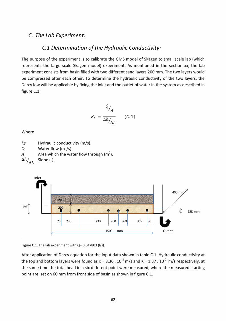
62

C. The Lab Experiment:

C.1 Determination of the Hydraulic Conductivity:

The purpose of the experiment is to calibrate the GMS model of Skagen to small scale lab (which

represents the large scale Skagen model) experiment. As mentioned in the section xx, the lab

experiment consists from basin filled with two different sand layers 200 mm. The two layers would

be compressed after each other. To determine the hydraulic conductivity of the two layers, the

Darcy low will be applicable by fixing the inlet and the outlet of water in the system as described in

figure C.1:

⁄

⁄ ( )

Where Ks Hydraulic conductivity (m/s). Q Water flow (m3/s). A Area which the water flow through (m2).

⁄ Slope (-).

Figure C.1: The lab experiment with Q= 0.047803 (l/s).

After application of Darcy equation for the input data shown in table C.1. Hydraulic conductivity at

the top and bottom layers were found as K = 8.36 . 10-3 m/s and K = 1.37 . 10-2 m/s respectively. at

the same time the total head in a six different point were measured, where the measured starting

point are set on 60 mm from front side of basin as shown in figure C.1.

Inlet

400 mm

195

128 mm

25 230 230 260 360 365 30

1500 mm Outlet

200

200

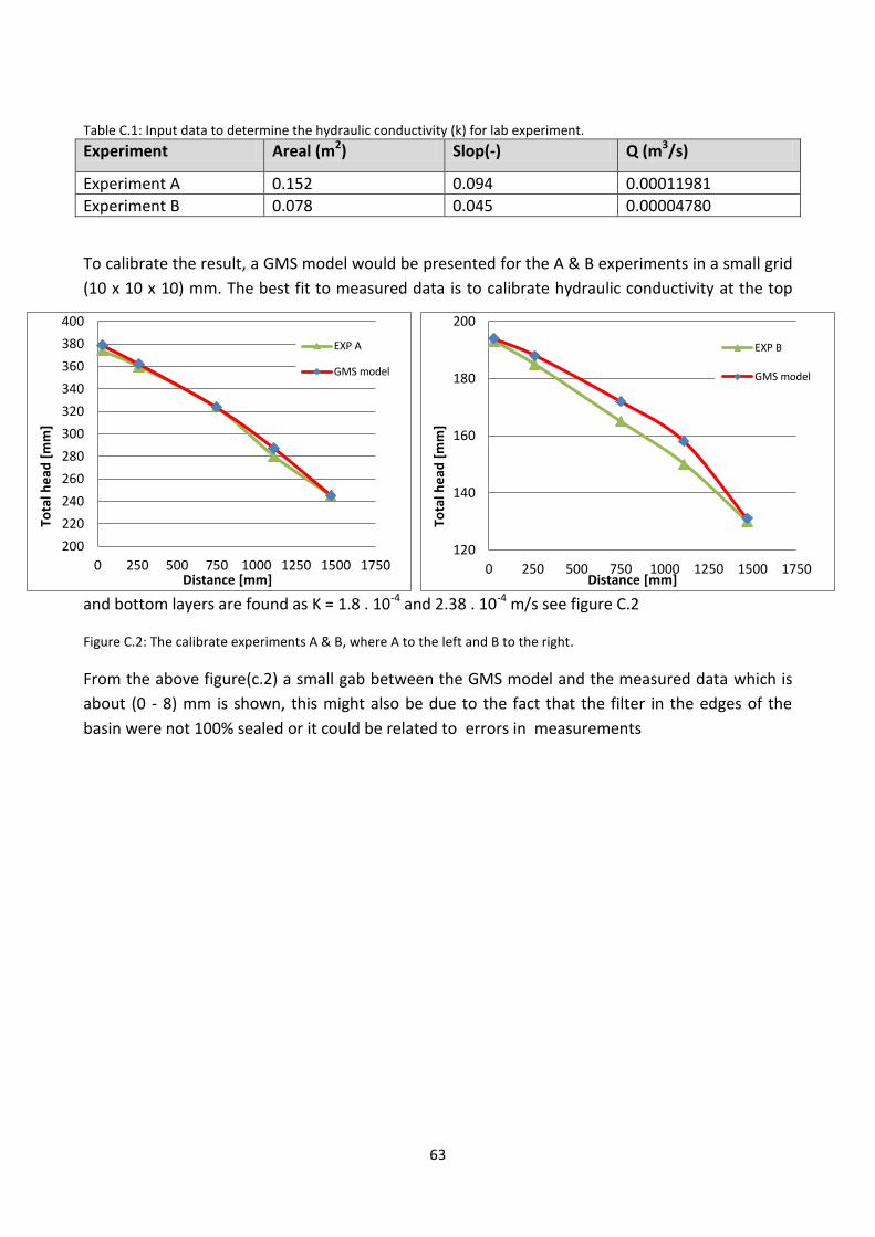
63

Table C.1: Input data to determine the hydraulic conductivity (k) for lab experiment.

Experiment Areal (m2) Slop(-) Q (m3/s)

Experiment A 0.152 0.094 0.00011981

Experiment B 0.078 0.045 0.00004780

To calibrate the result, a GMS model would be presented for the A & B experiments in a small grid

(10 x 10 x 10) mm. The best fit to measured data is to calibrate hydraulic conductivity at the top

and bottom layers are found as K = 1.8 . 10-4 and 2.38 . 10-4 m/s see figure C.2

Figure C.2: The calibrate experiments A & B, where A to the left and B to the right.

From the above figure(c.2) a small gab between the GMS model and the measured data which is

about (0 - 8) mm is shown, this might also be due to the fact that the filter in the edges of the

basin were not 100% sealed or it could be related to errors in measurements

200

220

240

260

280

300

320

340

360

380

400

0 250 500 750 1000 1250 1500 1750

Tota

l he

ad [

mm

]

Distance [mm]

EXP A

GMS model

120

140

160

180

200

0 250 500 750 1000 1250 1500 1750

Tota

l he

ad [

mm

]

Distance [mm]

EXP B

GMS model

64

C.2 Experiments with different pumping quantity:

To pumping with P2 =0.008969565 l/s

Figure B.3: The total measured head profile of the lab experiment when the pumping water P2 = 0.008969565 (l/s).

Figure B.4: The total GMS head profile in pump section of the lab experiment when the pumping water P2 =

0.008969565 (l/s).

Figure B.5: The result of the calibration of the lab experiment when the pumping water P2 = 0,008969565 (l/s).

240

260

280

300

320

340

360

380

0 200 400 600 800 1000 1200 1400 1600

Tota

l he

ad [

mm

]

Distance [mm]

P2

240

260

280

300

320

340

360

380

0 200 400 600 800 1000 1200 1400 1600

Tota

l he

ad [

mm

]

Distance [mm]

P2

GMS model

65

To pumping with P1 =0.012582955 l/s

Figure B.6: The total measured head profile of the lab experiment when the pumping water P1 = 0.012582955 (l/s)

Figure B.7: The total GMS head profile in pump section of the lab experiment when the pumping water P1 =

0.012582955 (l/s).

Figure B.8: The result of the calibration of the lab experiment when the pumping water P1 = 0,012582955 (l/s).

240

260

280

300

320

340

360

380

0 200 400 600 800 1000 1200 1400 1600

Tota

l he

ad [

mm

]

Distance [mm]

P1

240

260

280

300

320

340

360

380

0 200 400 600 800 1000 1200 1400 1600

Tota

l he

ad [

mm

]

Distance [mm]

P1

GMS model

water supply in skagen - modeling of...

Documents