Water temperature modeling in streams to support ecological restoration

By

Nathaniel L. Butler

A dissertation submitted in partial satisfaction of the

requirements for the degree of

Doctor of Philosophy

in

Engineering – Civil and Environmental Engineering

in the

Graduate Division

of the

University of California, Berkeley

Committee in charge:

Professor James R. Hunt Professor Mark Stacey Professor G.M. Kondolf

Summer 2015

1

Abstract

Water temperature modeling in streams to support ecological restoration

by

Nathaniel L. Butler

Doctor of Philosophy in Engineering – Civil and Environmental Engineering

University of California, Berkeley

Professor James R. Hunt, Chair

Water temperature is a critical water quality parameter that affects salmonid survival by influencing its metabolism and growth at all life stages. Stream temperature is an especially important parameter in California rivers where it frequently limits the range of salmonids. Anthropogenic activities have increased stream temperature and degraded spawning, holding, and rearing habitats, and this has contributed to declines in salmonid populations in California. Fisheries managers have a range of analytical and empirical tools available to assess and quantify elevated stream temperature conditions, but many of these tools do not focus on water temperature conditions at the spatial and temporal scales important to salmonids. My research focuses on assessing water temperature at the watershed and upwelling hyporheic scale which are critical to salmonid survival as stream temperature approaches thermal tolerances.

I developed a model to calculate water temperature at locations throughout a watershed to provide a method to evaluate the availability and connectivity of suitable thermal habitat throughout a stream network. The model used a linear weighted average of the maximum and minimum air temperatures of the current and 4 prior days. The weighting parameter is dependent upon upstream drainage area enabling the application of the model to both small tributaries and large mainstem streams. I used historical data from the Sonoma Creek, Napa River, and Russian River watersheds to develop, test, calibrate, and partially validate the model. Model results from Sonoma Creek and Napa River indicated it was generally able to estimate daily average water temperature within 1.5oC of the observed water temperature. Data from the Russian River highlighted the model was limited to streams without significant hydrologic modifications or geologic constraints that forced groundwater to the surface.

2

A 1-D advection dispersion heat transport model was developed to quantify the upwelling hyporheic temperature that provides cold water thermal refugia along a streambed for salmonids. I analyzed hyporheic temperature measured at five sites in a previous research program across sixteen kilometers of Deer Creek near Vina, California, to test, calibrate, and partially validate the model. At three sites, I found the 1-D advection and dispersion were the dominant heat transport mechanisms with model root mean square error less than 0.6oC. At two sites, the model was not applicable because modeling results indicated that surface flow rate variations, solar radiation, and multi-day flow paths also influenced the upwelling hyporheic temperature. Modeling was valuable for highlighting the contribution of these additional processes from that of 1-D advection dispersion. The availability of monitoring data over the summer-fall period was essential for modeling upwelling temperature dynamics along a semi-natural channel.

i

To Anne, Joe, Alf, and most especially Amanda:

Thank you for all the support and encouragement over the many years.

ii

TABLE OF CONTENTS

CHAPTER 1 Overview ............................................................................................................ 1

1.1 Introduction ............................................................................................................ 1

1.2 Life-cycle of Pacific Salmonids .................................................................................. 3

1.3 Declining Salmonids Populations .............................................................................. 6

1.4 Causes for Declining Salmonid Populations in California ........................................... 8

1.5 Influence of Water Temperature on Salmonids ....................................................... 10

1.6 Salmonid Strategies for Surviving High Water Temperature .................................... 11

1.7 Management of Thermally Impaired Salmonid Stream Habitat ............................... 12

1.8 Challenges to Addressing Thermally Impaired Stream Habitat ................................ 12

1.9 Objectives of the Dissertation................................................................................. 13

1.10 Organization of the Dissertation ............................................................................. 14

CHAPTER 2 Heat transport in the stream environment ........................................................ 15

2.1 Introduction .......................................................................................................... 15

2.2 Heat Transport Processes ....................................................................................... 18

2.2.1 Radiative Heat Transfer ................................................................................... 18

2.2.2 Sensible Heat Transfer .................................................................................... 19

2.2.3 Latent Heat Transfer ....................................................................................... 20

2.2.4 Advective and Diffusive/Dispersive Heat Transfer ........................................... 20

2.2.5 Flow and Heat Transfer through Porous Media ................................................ 21

2.2.6 Surface-subsurface exchange in streams ......................................................... 24

2.2.7 Influence of geomorphology on hyporheic flow ............................................... 25

2.3 Modeling Stream Temperature .............................................................................. 25

2.3.1 Surface water temperature modeling .............................................................. 26

2.3.2 Surface – subsurface exchange in stream temperature modeling ..................... 28

2.4 Statistical Evaluation of Stream Temperature Models ............................................ 28

2.5 Next Steps ............................................................................................................. 30

CHAPTER 3 Modeling the spatial distribution of stream temperature within watersheds ..... 31

3.1 Introduction .......................................................................................................... 31

3.2 Sonoma Creek Watershed ...................................................................................... 31

iii

3.2.1 Data ................................................................................................................ 33

3.2.2 Overview of Sonoma Data ............................................................................... 38

3.2.3 Modeling of Stream Temperature ................................................................... 42

3.3 Napa River Watershed ........................................................................................... 52

3.3.1 Data ................................................................................................................ 53

3.3.2 Overview of Napa Valley Data ......................................................................... 58

3.3.3 Modeling of Stream Temperature in Napa Valley ............................................ 61

3.4 Russian River Watershed ....................................................................................... 72

3.4.1 Data ................................................................................................................ 73

3.4.2 Water Temperature Modeling in Russian River Watershed .............................. 77

3.5 Comparison Between Watersheds ......................................................................... 83

3.6 Discussion .............................................................................................................. 84

3.7 Summary ............................................................................................................... 84

CHAPTER 4 Modeling hyporheic exchange using 1-D advection dispersion heat transport ... 86

4.1 Introduction .......................................................................................................... 86

4.2 Deer Creek Watershed ........................................................................................... 86

4.2.1 Study Area ...................................................................................................... 86

4.2.2 Tompkins 2006 Study ...................................................................................... 88

4.3 Data ...................................................................................................................... 91

4.4 Modeling ............................................................................................................... 93

4.4.1 Model Checking .............................................................................................. 94

4.4.2 Model Calibration and Validation .................................................................... 97

4.5 Results by River Mile (RM) ................................................................................... 100

4.5.1 RM 6.0 .......................................................................................................... 100

4.5.2 RM 9.9 .......................................................................................................... 103

4.5.3 RM 5.7 .......................................................................................................... 106

4.5.4 RM 5.0 .......................................................................................................... 110

4.5.5 RM 2.7 .......................................................................................................... 117

4.5.6 RM 6.9 ......................................................................................................... 123

iv

4.6 Discussion ............................................................................................................ 132

4.7 Summary ............................................................................................................. 136

CHAPTER 5 Conclusions .................................................................................................... 137

5.1 Summary ............................................................................................................. 137

5.2 Recommendations ............................................................................................... 139

REFERENCES ...................................................................................................................... 140

v

Acknowledgements

Many people have my deepest gratitude for their contributions to making my research and this dissertation a reality. First, I want to thank my qualifying and dissertation committees. Thank you to my advisor, Jim Hunt, for the freedom to pursue many different research interests during my Ph.D., his many thoughtful insights, and his unwavering dedication to refined simplicity. I learned an enormous amount having you as a mentor. Thank you to Mark Stacey for all his guidance, encouragement, and feedback. Thank you to Matt Kondolf for being an inspiration and helping me throughout my Ph.D. program. His class during my Master’s program solidified my dedication to river restoration and salmonids. Thank you to Stephanie Carlson for her many hours and invaluable help understanding salmonid biology and life-histories. I am also enormously grateful to Stephanie for her support in my early research on John West Fork. Thank you to Evan Variano for his many strategies and ideas for designing experiments.

I also want to thank all the people and organizations that have supported me and my research over the years. Thank you to the National Science Foundation Graduate Research Fellowship Program which funded me early in the Ph.D. program. Thank you to Charlotte Ambrose and the National Marine Fisheries Service (NMFS) for the inspiration and support researching stream temperature in ungauged watersheds. The model developed in Chapter 3 began with the work supported by Charlotte and NMFS. Thank you to Carolyn Remick, Deb Agarwal, the Berkeley Water Center, and Microsoft Research which funded the digital watershed project at the Berkeley Water Center. Much of my work investigating stream temperature across watersheds was made significantly easier thanks to the California Datacube. Most especially thank you to Mark Tompkins for sharing his data, his time, and his insights into hyporheic exchange at Deer Creek. I also want to thank Katrina Harrison, Dave Mooney, Michelle Banonis, Ali Forsythe, and everyone at the San Joaquin River Restoration Program for their support of my research.

Thank you to Joan Chamberlain, Shelley Okimoto, Robert Harley, Slav Hermanowicz, and all those in the Civil and Environmental Engineering Department who helped me throughout my time at U.C. Berkeley. Thank you to all the teachers who had me as a Graduate Student Instructor. Thank you to my office/department mates for keeping things fun and being there to talk through ideas, especially Steve Gladding, Arthur Wiedmer, and Wayne Wagner.

Finally, thank you Mom, Dad, Alf, and Amanda for encouraging me, believing in me, and keeping me grounded during these many years. A big thank you to Amanda for all her patience, support, and understanding during the many months I spent writing this dissertation. Thank you to all my friends who brought so much joy into my life over the years: Alex, Quynh, Anita, Mike, Arthur, Ashley, Aspan, Gwen, Hai Yen, Lisa and my E7 students, Mario, Mai, Mehershad, Mildred, Nancy, Andre, Tianna, and Wynne. A special thank you to Alex Polyakov for the many cofftea breaks discussing research, life, the universe, and everything. Thank you to Diana, Vivian, Piotr, JKong, Jennifer, Anh, Christine, and the rest of the VSA for the culture and karaoke. Lastly, thank you to Survay Says! and Kill Lincoln for awesome concerts at 924 Gilman and providing a soundtrack to much of my life these past years.

1

CHAPTER 1

Overview

1.1 Introduction

Salmon leaping up cascading streams is one of the defining images of picturesque wild streams. This vision of the migrating adult salmon is but one stage in a complex life history that encompasses years over both large and small streams along with the vast ocean. As anadromous fish, Pacific salmonids are born in freshwater streams, spend some portion of their life rearing in freshwater streams, migrate to the ocean to mature to adulthood, and finally return to freshwater to spawn. Due to the complexity of the Pacific salmonid life history, salmonids are vulnerable to environmental changes at a range of spatial and temporal scales. Severely declining salmonid populations in California and the Pacific Northwest during the past decade prompted fisheries managers to scrutinize stream water quality to protect salmonids and their habitats. Degraded stream habitat and water quality have extirpated salmonids from much of their historical habitat and contributed to severely declining salmonid populations in California and the Pacific Northwest during the past decade (Figure 1). Alterations in water flow, flow timing, sediment loads, stream access, ocean access, riparian cover, water temperature, and numerous other environmental factors have degraded salmonid stream habitat and water quality. While all parameters influence salmonid survival, water temperature is a critical parameter that affects salmonids at all life stages by directly influencing salmonid metabolism and growth. A range of analytical and empirical tools are used to assess and quantify elevated stream temperature conditions, but environmental resource managers still struggle with assessing water temperature. My research focuses on assessing water temperature at two different scales important to salmonids within thermally impaired streams. First, I develop an empirical model to assess the basin scale trends in stream temperature critical for salmonid migration and rearing. Second, I model hyporheic exchange to improve understanding of the processes that contribute to the creation of thermal refugia in streams through monitoring data analysis followed by quantitative modeling. Together these two studies address the needs of fisheries managers for better ways of assessing stream water temperature conditions at two spatial scales important for fisheries.

2

Figure 1: Historical and current distribution of salmonids in California (Howard et al., 2011).

Study area in the figure is from Howard et al. (2011) and does not apply to studies in this

dissertation.

3

1.2 Life-cycle of Pacific Salmonids

The life-history of salmonids can be divided into four distinct periods based on the environment the salmonid occupies (Figure 2). First is the streambed gravel period where the salmonid develops from a freshly laid egg to an alevin and then emergences from the gravel as fry. Next is the first free-swimming freshwater stream period where the juvenile salmonid rears until growing to a suitable size that it can smolt and migrate towards the ocean. The third period is dominated by residency in the ocean where the salmonid smolt grows into an adult. The fourth and final period is a second freshwater stream period where the adult, sexually mature salmon migrates upstream to spawn in its natal stream where it first hatched as an egg.

Figure 2: Schematic of Pacific salmonid life-cycle (adapted from USFWS, 1995).

The life-cycle of the salmonid begins with the streambed gravel period where adults bury their eggs in gravel nests called redds along cool, well-oxygenated streambeds. Eggs incubate in the gravels for a period of time determined primarily by the water temperature but also by the dissolved oxygen levels in the water. Salmonids are ectothermic so their developmental rate

Streambed

Stream

Ocean

Stream

4

and metabolism increase with temperature. Eggs require a certain amount of cumulative warmth to initiate hatching usually listed as the number of “degree days” or “temperature units” (TUs) until they hatch. This variation in the timing of hatching has enabled salmonids to spawn in either fall or spring but still have eggs hatch at similar times when stream conditions are optimal for growth, migration, and survival. Dissolved oxygen levels contribute to the number of days until eggs hatch by determining how well the respiratory demands of the eggs are met. Low dissolved oxygen levels increase the number of days until eggs hatch and reduce the size of hatched alevin. Once eggs hatch, the alevins swim deeper into the gravel streambed to hide until they absorb their yolk sacs. Water temperature and dissolved oxygen again play an important role by determining how quickly and efficiently the yolk sac is absorbed and how much alevins grow. Higher water temperature and lower dissolved oxygen increase metabolic demands, so alevins grow less. Under low dissolved oxygen, alevin will be forced to migrate laterally through the gravel streambed further reducing the yolk that can be converted into growth. After the yolk is fully absorbed, alevins emerge from the gravel as fry and disperse upstream or downstream to establish territories that they can use as rearing parr juveniles. Parr juveniles are distinguished by their camouflage of spots and vertical bars called parr marks along their sides.

Different salmonids exhibit different life-histories as juveniles, but all species have a free-swimming period where they utilize stream habitats for growth before migrating to the ocean. Juvenile salmonids select stream habitats to optimize growth by balancing food availability with the energy cost of obtaining it. Each salmonid species has definable stream habitat preferences that range from shallow, fast-moving water near riffles for Steelhead to deep, slow-moving water in pools for Coho. Habitat preferences are not fixed and vary with time of year, body size, competition with other salmonids, food availability, and water quality. Salmonids will abandon habitats and seek out new ones if conditions become unfavorable for growth. Salmonids spend anywhere from a few months to three years in streams feeding and growing before eventually migrating towards the ocean.

Migration to the ocean is hardwired into many salmonid species, but the range of ages that salmonids begin the migration indicates flexibility in timing. Generally, migration to the ocean is undertaken only once the juvenile has reached a certain size threshold. Stream conditions directly influence the proportion that migrates each year by influencing growth and whether the juvenile can grow to meet the threshold to migrate to the ocean. Larger size increases ocean survival odds, but every year in freshwater poses mortality risk due to food limitations, high summer water temperatures, predation, and low stream flow conditions. Juveniles that have reached the threshold size needed for migration to the ocean begin the journey during spring as environmental conditions in the stream become less optimal for growth, stream flow increases to enable passage downstream, and marine conditions become optimal for growth (Quinn, 2005). Water velocity, day of the year, the location from which fish begin migration, fish size, extent of parr juveniles-smolt transformation, and environmental conditions all affect the downstream migration rate. Peak migration occurs when stream discharge peaks though the relationship between migration rate and discharge varies with fish response to velocity and habitat preference. At low stream velocities, salmonids may swim downstream faster than the

5

water velocity, while at higher velocities salmonids may move more discontinuously. Poor stream conditions may further alter migration behavior by creating flow and water quality barriers that salmon cannot pass (Madej et al., 2006). As salmon migrate downstream, their biology transforms from parr juveniles to smolts preparing them for the ocean environment. Ion regulation, color, body morphology, metabolic and endocrine adjustments, and multiple other biological changes occur during downstream migration as they adapt to ocean conditions. As a final stage before entering the ocean, smolts spend time in estuaries to grow and utilize the range of salinities to select optimal conditions as they complete their adaptation to ocean conditions (Quinn, 2005). Length of estuary occupancy varies between species with Chinook spending more time in estuaries progressively shifting to higher salinity water, while Coho move rapidly through estuaries (Healey, 1980; McCabe et al., 1986; MacDonald et al., 1987).

Once in the ocean, salmonids spend one to four years growing before returning to their natal stream to spawn. Genetic controls, smolt size, and ocean conditions all influence the age salmonids reach maturity with rapidly growing salmonids reaching maturity sooner. Poor ocean conditions that reduce food availability increase the time salmonids need to mature. As salmonids approach sexual maturity, they use a combination of orienting their movements with respect to the sun’s transit across the sky, the plane of polarization of light, and the magnetic field of the earth to navigate back to their natal stream’s coastal region (Quinn, 2005).

The final period the salmonid life-cycle begins when salmonids reenter freshwater streams to begin their upstream migration to their natal spawning grounds. Salmonids during this period swim upstream from less than a kilometer to thousands of kilometers through complex stream networks across a range of stream conditions to return to their birth stream. The homing behavior of salmonids to return to their natal stream to spawn is a key component of the salmonid life-cycle shared by 95-99% of all adults. Salmonids home to their natal streams using magnetic field orientation and learned odor memories from the period they spent in streams before migrating to the ocean. While only a small percentage of salmonids stray from spawning in their natal stream, those salmonids play an important evolutionary role at colonizing any viable stream habitats and spreading genetic diversity. Timing of upstream salmonid migrations is most strongly controlled by genetic factors that have selected the salmonids that return during the most favorable long-term average conditions of their natal streams (Siitonen and Gall, 1989; Quinn and Adams, 1996). Timing variations in upstream migration between populations and species corresponds to constraints on suitable environmental conditions for upstream migration, physical access to spawning grounds, and a suitable number of “degree days” so eggs hatch when stream conditions are optimal for juveniles. Upon reaching natal spawning grounds, salmonids prepare redd nests, lay their eggs, and then guard their redd from disturbance by other spawning salmonids. All salmonid species except O. mykiss are semelparous so after a period of guarding their redd, salmonids die with their bodies providing nutrients to the stream and surrounding landscape.

6

1.3 Declining Salmonids Populations

Salmonid fishery resources in the Pacific Northwest and California are dramatically declining with many once plentiful salmonid populations now being listed as threatened or endangered by the Endangered Species Act (Nehlsen et al., 1991; Moyle et al., 1995; Watanabe et al., 2005; Roni et al., 2008). Declines in salmonids threaten the genetic reservoir upon which the future evolutionary potential and viability of salmonids will depend as climate conditions change. Preservation of the genetic resources of southern salmonid populations in California is especially critical because these populations are adapted to warmer climactic conditions (Moyle et al., 2008). There are two main scales of concern for preserving the genetic reservoir of salmonids. The smallest scale of concern in the Endangered Species Act is the population. Salmonids are grouped into populations by their tendency to spawn in a particular locality at a particular season and not to interbreed substantially with salmonids from any other group (Bjorkstedt et al., 2005). Populations are not reproductively isolated from each other with genetic exchange occasionally occurring between populations as individuals stray between spawning streams. Populations are grouped into Evolutionarily Significant Units (ESUs) that are reproductively isolated and represent an important component of the evolutionary legacy of the species (Moyle et al., 2008). Each ESU has unique genetic variability produced by past evolutionary events to adapt the salmonid to its set of local environmental conditions. Conservation of the genetic resources of each ESU is a priority of the Endangered Species Act to ensure that salmonid evolution is not genetically constrained.

Declining salmonid populations also have measureable ecosystem and economic consequences. Reduced salmonid populations threaten ecosystem productivity as fewer nutrients are transported upstream. Salmonids migrating upstream to spawn transport marine nutrients from their growth in the Pacific Ocean (Cederholm et al., 1999). Richey et al. (1975) showed that salmonid spawner abundance altered the amount of nutrients released by comparing the nutrient contribution from different sizes of spawning runs in the same system. Stable isotope analysis of 13C and 15N has verified that marine derived nutrients from salmonid carcasses enhance watershed productivity (Mathisen et al., 1988). Kline et al. (1993) found higher stable isotope ratios of 15N in the biota of systems with anadromous salmon than systems without salmon. Increased 15N from a controlled salmonid carcass experiment increased tree growth and riparian productivity in a study of 11 small to medium sized streams in British Columbia (Hocking and Reynolds, 2012). Reductions in salmonid spawners is hypothesized to reduce the overall productivity of watersheds (Gresh et al., 2000; Wipfli et al., 2003; Wipfli et al., 2004; Cram et al., 2011). The continued decline of fishery resources also threatens severe social and economic consequences (Nehlsen et al., 1991; Frissell et al., 1996). The salmon fishing moratorium in 2008 and 2009 resulted in a direct annual economic loss of millions of dollars (BFC, 2010).

Salmonid species in California are especially imperiled with numerous populations reaching record low numbers (Nehlsen et al., 1991; Myers et al., 1998; NMFS, 2012). A comprehensive analysis of the status of California salmonids in 2008 found that 59% of the anadromous salmonids were in danger of extinction. Based on current trends, the analysis estimated that

7

65% of California salmonids would be gone within 50 - 100 years (Moyle et al., 2008). Declines in salmonid populations reached a critical junction in 1989 when only 550 winter-run Chinook returned to the Sacramento River at Red Bluff. The winter-run Chinook population averaged 86,500 adults at Red Bluff between 1967 and 1969 so the historically low return in 1989 prompted the National Marine Fisheries Service (NMFS) to take action to protect salmonids. By the end of 1990, the Sacramento River winter-run Chinook salmon were the first salmon population listed as threatened under the Endangered Species Act and endangered by the state of California (Nehlsen et al., 1991). Declines in other salmonid populations around California since 1990 also spurred action and protection by the Endangered Species Act. Most California Steelhead populations have been listed as threatened or endangered under the Endangered Species Act (Jackson, 2007). Figure 3 shows that estimates of historic California Coho populations statewide indicate that Coho numbers have declined by approximately 95% in the past 50 – 60 years with both ESUs in California being listed as threatened or endangered (Moyle et al., 2008; NMFS, 2012). The abundance of Chinook populations have declined significantly from historic levels, but abundance trends for the different populations of Chinook have varied widely. Conservation measures have increased Central Valley winter-run Chinook numbers to an average 8,100 adult spawners per year with an estimated annual population increase of 28% (Moyle et al., 2008). Between 1992 and 2005 Central Valley fall-run Chinook populations were generally stable at around 450,000 fish per year, but abundance has recently plummeted to historic lows (Moyle et al., 2008; Lindley et al., 2009). A complete closure of commercial and recreational Chinook salmon fisheries was imposed for all of California in 2008 and 2009 by the Pacific Fishery Management Council because Chinook salmon returns were at historic lows with only 66,000 adult spawners returning in 2008 (Lindley et al., 2009; PFMC, 2010).

Figure 3: Historical estimates of Coho salmon spawners (NMFS, 2012).

8

1.4 Causes for Declining Salmonid Populations in California

Pacific salmonids require a variety of habitats to complete their lifecycle and reproduce. Disruption or destruction of any one of these habitats or environments reduces a population’s viability. Ocean conditions, stream habitat, water quality, introduced and/or artificially propagated fish stocks, land use, and overfishing are all frequently cited as the primary causes for declining salmonid populations (Myers et al., 1998; Moyle et al., 2008; NMFS, 2012). Ocean conditions are critical to salmonid survival, but fluctuate stochastically with inter-annual and decadal-scale processes like the El Nino Southern Oscillation and the Pacific Decadal Oscillation (NMFS, 2012; Wainwright and Weitkamp, 2013). Conditions that decrease ocean productivity are believed to be responsible for low ocean survival of salmon (Barth et al., 2007), but the relationship between ocean productivity and salmon survival is poorly understood (Moyle et al., 2008). While ocean conditions affect adult salmonid survival, poor freshwater habitat conditions are the primary cause for declines in salmonid population and compromising their resilience to ocean variability (NMFS, 2012).

Much of the decline in California salmonid numbers is attributed to anthropogenic activities that eliminated or degraded stream habitat needed by salmonids for different life stages (Moyle et al., 2008; Lindley et al., 2009; Beer and Anderson, 2013). An extensive review of all the different factors causing the decline of each salmonid population in California identified numerous human activities contributing to declines in salmonid populations since no one factor was entirely responsible (Moyle et al., 2008). Moyle et al. (2008) detailed how a combination of many different factors and their non-linear total impact degraded salmonid habitat leading to the currently low population numbers in California. The top five factors listed as affecting anadromous salmonid populations in California were dams (impacting 75% of the California populations), hatcheries (75%), logging (70%), water diversions (65%), and commercial and recreational fisheries (65%). Other anthropogenic activities that were frequently listed included urbanization, agriculture, mining, and stream modifications for flood protection.

Dams chiefly block access to upstream habitat, alter downstream flow patterns, and change water quality. Central Valley salmonid populations have been especially impacted by dams. Yoshiyama et al. (1996) estimated that 48% of historic salmonid stream habitat used for spawning, holding, or migrating in the Central Valley basin has been lost primarily from dam construction and flow diversions. Moyle et al. (2008) explained how 90% of spring-run Chinook salmon historic stream habitat was blocked by Central Valley dams and resulted in spring-run Chinook population declines. Dams can also have negative effects on downstream spawning and rearing habitat. Gravel needed by salmonids for laying eggs is trapped behind dams which degrades spawning habitat below dams. Dams can alter the thermal regime of streams by releasing warmer surface water during summer months. Both the downstream migrating smolts and upstream migrating adults are negatively affected by reductions in peak stream flows and variations in their timing. In a synthesis of the literature, Poole and Berman (2001) demonstrated reductions in peak flows also change the geomorphic controls that shape the river and this reduces stream complexity and ultimately the available juvenile rearing and adult holding habitats.

9

Hatcheries have negatively impacted salmonid populations by displacing wild populations and decreasing genetic diversity that reduce the fitness of wild populations. Releases of large numbers of hatchery salmonids into a stream reduces food availability for native species leading to negative competitive interactions that reduce wild populations (Nickelson et al., 1986; Spence et al., 1996). Increased competitive behavior and reduced food availability combine to reduce growth rates so salmonids entering into the ocean are smaller and more vulnerable to predation (Moyle et al., 2008). Hatcheries are also believed to reduce salmonid populations by mingling the genetics of different salmonid populations (Williams, 2006). Studies of hatchery raised salmonids indicate that they are less able to produce young that survive to reproduce (Araki et al., 2007). The genetic effects of hatchery salmonids reproducing with wild populations have contributed to the decline in California salmonid populations (Waples, 1991; Moyle et al., 2008).

Logging contributed to declining salmonid populations by severely degrading spawning, incubation, and rearing habitat. Much of logging’s worst damage to stream habitat occurred during the 19th and early 20th century when splash and crib dams were used to transport logs from harvest sites to downstream sawmills. These small, temporary dams stored enough water to eventually float logs downstream, but they blocked upstream salmonid passage and scoured away downstream habitat when they were breached. Logging, splash dams, reductions in riparian vegetation, and increased erosion from road building all increased the sediment input into streams. This additional sediment reduced stream complexity by burying suitable spawning habitats, filling critical pool rearing habitats, and widening stream channels. Removal of riparian vegetation and woody debris from stream channels combined with shallower water flows also caused increased water temperature. Logging further degraded stream habitat because less riparian vegetation reduced food availability in streams by simplifying aquatic food webs (Moyle et al., 2008; NMFS, 2012).

Water diversions negatively impact salmonid populations primarily by reducing stream flows during critical times, degrading water quality, and entraining migrating juveniles. Reduced flows degrade habitat, increase salmonid mortality by dewatering stream habitat, increase summer water temperatures, and increase deposition of fine sediments (NMFS, 2012). Reduced stream flows from both large dam diversions along with smaller agricultural or residential diversions impact salmonid survival at multiple locations in California. Water diversions from Friant Dam combined with smaller diversions along the San Joaquin River dewatered 60 miles of the San Joaquin River between the Friant Dam and the confluence with the Merced River (Yoshiyama et al., 1996). The dewatering of the San Joaquin River is cited as the primary cause of the extirpation of its Chinook salmon populations. Diversions from the Shasta River resulted in the historically cold tributary becoming warmer than the thermal tolerances of most salmonids (Moyle et al., 2008). In the Klamath River, increased summer water temperatures from low flows increased adult mortality (Moyle et al., 1995). Water diversions also impact stream water quality when water diverted for agriculture returns to the river warmer and polluted with animal waste, higher nutrients and other toxics (Moyle et al., 2008). In tributary creeks of the Russian River, diversions for frost protection in vineyards reduced stream flow by as much as 95% over a period of hours dewatering riffles and

10

potentially causing salmonid mortality (Dietch et al., 2008). Diversions also cause mortality of salmonids by entrainment. The federal Central Valley Project and the State Water Project are estimated to have a maximum 10% mortality of juvenile Chinook when entrained juveniles are salvaged and released downstream into predator-rich waters (Kimmerer, 2008).

Harvest of salmonid populations during recreational and commercial fishing has contributed to salmonid population declines though regulation of fisheries is reducing its impact (Williams, 2006). The commercial harvest of larger, older Chinook salmon that produce more eggs per female has resulted in spawning runs of mainly three-year-old salmon. Spawning runs comprised of only one age class are vulnerable to population crashes when natural conditions like drought result in poor survival one year. A diversity of age classes enable spawning runs to repopulate more easily (Moyle et al., 2008).

While there have been many human activities that contribute to declining salmonid populations in California, human activities frequently increase stream water temperature degrading spawning, holding or rearing habitat. In the review of factors affecting salmonid populations, increased water temperature was referenced as a detrimental outcome of human activities for 80% of salmonids populations (Moyle et al., 2008). Human activities have increased water temperature in some streams so much that thermal barriers are created preventing migration or leading to salmonid mortality (Strange, 2010). Water withdrawals from the Eel River to the Russian River create thermal barriers in the upper mainstem Eel River in early spring restricting juvenile migration (Moyle et al., 2008). Anthropogenic increases in water temperature are one of the primary reasons for impaired stream habitat quality for salmonids (Lichatowich, 1999; USEPA, 2003; Watanabe et al., 2005). The Federal Clean Water Act under Section 303(d) and 305(b) requires the California State and Regional Water Boards to list of all the water bodies with impaired water quality in California. While only 15.8% of streams in California have been assessed, Section 303(d) data can be used to approximate the frequency with which water temperature impairs water quality. Fifty-one percent of the river miles assessed were impaired due to water temperature and water temperature was the number one cause of impaired water quality based on the recent Section 303(d) list data from 2010 (USEPA, 2015). Water temperature is projected to become an even more frequent source of water quality impairment for salmonids in California with expected climate change (Beer and Anderson, 2013).

1.5 Influence of Water Temperature on Salmonids

Water temperature is an important water quality parameter for aquatic ecosystems because of its influences on primary producers, macroinvertebrates, and salmonids (Huntsman, 1942; Hynes, 1970; Sweeney and Vannote, 1986; Ward, 1992; Sullivan et al., 2000; Wagner et al., 2010). Each salmonid life stage and population has specific water temperature tolerances determined by genetic variations suited to local conditions (Moyle et al., 2008; Strange, 2010). While the literature remains divided, researchers are beginning to question whether studies of thermal tolerances in more northern salmonid populations are applicable to southern salmonid populations. Southern juvenile Steelhead were found to persist in rivers where daily water temperature ranged from 17.4oC – 24.8oC (Spina, 2007) and where peak temperature reached

11

25 – 28°C (Carpanzano, 1996; SYRTAC, 2000), yet literature drawn primarily from more northern Steelhead populations reported the preferred temperature of juvenile Steelhead as 10 – 17°C (Moyle et al., 2008). Water temperature directly influences almost every aspect of the life history of salmonids including metabolism, behavior, and migration (Beschta et al., 1987; Groot et al., 1995; Spence et al. 1996; Berman, 1998). Salmonids are ectothermic so water temperature influences salmonid survival by affecting the efficiency of salmonid metabolism and growth. Water temperatures greater than physiological optimums reduce growth, increase susceptibility to disease, and lead to higher mortality rates (Fry, 1971; Torgersen et al., 1999; Sullivan et al., 2000; Madej et al., 2006). Higher water temperature also negatively impacts other water quality parameters critical to salmonid survival. Warmer water lowers the solubility of dissolved oxygen hindering salmonid respiration (Ficklin et al., 2013). High water temperature also creates thermal barriers that render upstream habitat inaccessible (Matthews and Zimmerman, 1990; Ebersole et al., 2001; Strange 2010). Juvenile rearing, adult migration, and adult holding are the life stages most vulnerable to variations in water temperature because these life stages occupy stream ecosystem from late spring through early fall months when stream temperatures peak.

1.6 Salmonid Strategies for Surviving High Water Temperature

Salmonids modify their behavior when ambient stream water temperatures exceed temperature tolerances (Li et al., 1993; Nielsen et al., 1994; Matthews and Berg, 1997; Ebersole et al., 2003). Salmon seek out thermal refugia where local stream water temperature is cooler than ambient stream water temperature (Nielsen et al., 1994; Torgersen et al., 1999; Ebersole et al., 2003). Vertical water temperature gradients or thermal stratification in pools can create thermal refugia enabling salmonids to select water temperatures that balance their thermal tolerances with food availability, dissolved oxygen, and holding behavior (Gibson, 1966; Keller and Hofstra, 1983; Nielsen et al., 1994; Matthews and Berg, 1997; Ebersole et al., 2001, Ebersole et al., 2003). Salmonids primarily occupy thermal refugia during the hottest parts of the day when ambient water temperatures approach the lethal limit (Frissell et al., 1996; Matthews and Berg, 1997; Ebersole et al., 2003). Studies found that salmon preferred cold water refugia in thermally stratified pools (Keller and Hofstra, 1983; Nielsen et al., 1994; Matthews and Berg, 1997; Tate et al., 2007), yet Frissell et al. (1996) and Ebersole et al. (2003) observed salmonids occupying cold water patches along bars and riffles. In 1942 once upstream habitat was cut off by Friant Dam construction, spring-run San Joaquin River Chinook salmon were found holding in pools below the Friant Dam to survive summer water temperatures greater than 22°C (Yoshiyama et al., 1996). Salmonids were observed traveling up to 25 m to take advantage of cold water refuge, though it is believed they will travel much greater distances (Li et al., 1993; Nielsen et al., 1994; Ebersole et al., 2001). If the demand for thermal refugia exceeds the capacity, salmonids may be forced to migrate significant distances or perish (Ebersole et al., 2001). In addition to providing suitable water temperature at specific

12

locations, sufficiently spaced thermal refugia also longitudinally connects habitat (Ebersole et al., 2003).

1.7 Management of Thermally Impaired Salmonid Stream Habitat

Water temperature that threatens salmonid survival is addressed by environmental resource managers primarily through the provisions of the Endangered Species Act and the Clean Water Act. Once a salmonid species is listed by the Endangered Species Act, federal, state, and local agencies are directed to protect and restore the species. A recovery plan is required to focus and prioritize threats and restoration actions needed to recover a salmonid species. The National Oceanic and Atmospheric Administration’s (NOAA) National Marine Fisheries Service (NMFS) in cooperation with other agencies and stakeholders is required to develop this recovery plan. One of the first steps in recovery planning is to assess historical and current stream conditions to develop realistic restoration goals. Historical salmonid populations are estimated using the NMFS’s Intrinsic Potential model (Agarwal et al., 2005) and the recovery plan develops restoration actions to improve water temperature in thermally impaired streams along with the many other factors contributing to salmonid population declines (NMFS, 2012).

Management of thermally impaired stream habitat is also supported by the Clean Water Act which regulates water quality standards including stream temperature (Poole et al., 2001; Allen et al., 2007). The Clean Water Act requires states to determine whether water bodies meet water quality standards that maintain beneficial uses for surface waters including protecting salmonids and other threatened or endangered species. When water temperature exceeds salmonid thermal tolerances in a stream and threatens their survival, the Clean Water Act Section 303(d) requires that the stream be listed as an impaired water body. When the Klamath and Shasta Rivers were listed on California’s 303(d) List of Impaired Water Bodies due to high water temperatures, the Clean Water Act required local agencies to develop water quality standards to assist in management and restoration actions (Flint and Flint, 2008).

1.8 Challenges to Addressing Thermally Impaired Stream Habitat

While much is being done to improve stream habitat conditions for salmonids, environmental resource managers are limited in their tools for the assessment of current and historical thermal conditions. One challenge frequently facing environmental resource managers is a lack of sufficient water temperature data within watersheds that are being assessed. This difficulty of determining the water quality in all California streams means only 16% of streams have been assessed (USEPA, 2015). Monitoring programs are not able to fully sample all aquatic environments within watersheds under the range of conditions that determine water temperature suitability. Under these circumstances a combination of selective monitoring and modeling is required for estimating water temperature conditions.

13

Current models struggle to quantify the thermal suitability of aquatic habitats at two scales important to salmonids. At the watershed scale, stream temperature models have been developed (Brown and Barnwell, 1987; Sinokrot and Stefan, 1993; Mohseni et al., 1999; Bartholow, 2000; Allen et al., 2008), but existing models require extensive data inputs, require considerable effort to calibrate and validate, and are frequently region specific. These requirements make existing temperature models often impractical for fisheries managers with limited resources where temporal and spatial resolution is needed. There is thus a need for relatively simple methods of modeling stream temperature using readily available data. The NMFS currently assesses stream thermal habitat availability through a broad-scale intrinsic potential model. In the model, an air temperature map using PRISM, an air temperature interpolation data product, is generated first. The lowest August air temperature (LMAT) is then correlated with historical data of salmonid presence to identify an air temperature threshold above which salmonids are not found in streams. Areas with an air temperature above the threshold have their intrinsic potential score zeroed out to indicate the stream habitat is not suitable (Agrawal et al., 2005). Water temperature is never estimated by the model. The intrinsic potential model provides an estimate of suitable thermal habitat only at a broad watershed scale because the air temperature estimate has a spatial resolution of 2 km by 2 km and it is unable to provide stream-specific or reach-specific estimates of water temperature that would benefit historical population estimates, recovery plans, and restoration activities. Water temperature models at the pool-riffle scale share the limitations of watershed scale models, but also struggle to estimate critical thermal stream habitat including vertical temperature gradients salmonids use to behaviorally thermoregulate. Numerous studies show salmonids use vertical water temperature differences like those created by upwelling subsurface flow to survive otherwise lethal stream temperatures, but most models do not consider them for two key reasons. First, models do not attempt to estimate vertical temperature gradients because the time scale of modeling is longer than the duration of vertical temperature gradients. Most models determine water temperature at daily, weekly, or monthly time scales while vertical water temperature gradients in streams form and are dissipated on a daily time scale. Second, the processes that control vertical water temperature gradients in streams are poorly known. Subsurface-surface water exchange is a key process identified in the fisheries literature, but is not incorporated into stream temperature models given uncertainties in mechanisms and subsurface heterogeneities (Ebersole et al., 2003; Arrigoni et al., 2008; Burkholder et al., 2008). While there is recognition that subsurface-surface water exchange occurs and creates critical cold water refugia in streams, a quantitative understanding suitable for incorporation into predictive models is lacking (Ebersole et al., 2003; Watanabe et al., 2005).

1.9 Objectives of the Dissertation

The primary objective of this dissertation is to develop methods to assess the thermal habitat of streams at two scales critical to salmonid migration, rearing, and holding. This dissertation

14

presents two separate studies that together address the needs of environmental resource managers to estimate historical, current and future thermal habitat in streams. The studies focus on two different locations because no one region had the combination of data over the range of stream sizes and duration of monitoring data needed to test and validate models for stream temperature. At the watershed scale, my first study focused on the Sonoma Creek, Napa River, and Russian River watersheds with multiple years of data across a range of basin sizes to develop a model that estimates daily water temperature. While the Intrinsic Potential model used by NMFS could provide a broad-scale estimate of stream temperature across watersheds, it could not estimate specific stream temperatures with its coarse spatial resolution. The model developed in this first study takes the next step in estimating water temperature by combining air temperature with the upstream drainage area to determine daily average water temperature for individual streams along their entire length. The second study is at the pool-riffle scale and uses nearly continuous subsurface-surface water temperature data at Deer Creek near Vina, California, to model the upwelling temperature and subsurface flow rates. In modeling upwelling temperature, the Deer Creek study also reveals how surface flow influences subsurface-surface water exchange and the creation of thermal refugia.

1.10 Organization of the Dissertation

This chapter introduced the key background about salmonids, their declining populations, and the challenges faced by environmental resources managers in assessing habitat conditions and guiding restoration activities for salmonids using examples from California streams. While there are many reasons given for the decline in salmonid populations in California, water temperature is the focus of this research since it impairs more stream miles than any other water quality parameter. Neither monitoring data nor current predictive models are able to quantify thermal habitats within watersheds and more locally at the pool-riffle scale suggesting a need for the integration of monitoring data with process-based modeling for assessing thermal habitat for fisheries. The remainder of the thesis is organized to address the two studies of thermal regimes critical in assessing salmonid thermal habitat. Chapter 2 provides an overview of heat transport in surface streams and the subsurface. Chapter 3 utilizes extensive monitoring data available in the Napa River, Sonoma Creek, and the Russian River to develop, calibrate, and partially validate a daily stream temperature model throughout these watersheds as a function of only daily values of maximum and minimum regional air temperatures. Chapter 4 utilizes a unique set of surface and subsurface water temperature data to develop, calibrate, and partially validate a model for upwelled water temperature that locally determines thermal refugia on an hourly basis. The last chapter provides a summary of the thesis, an integration of the two separate studies, and speculation on challenges remaining in improving thermal habitat assessment for aquatic habitat restoration.

15

CHAPTER 2

Heat transport in the stream environment

2.1 Introduction

Water temperature is an important determinant in the survivability of salmonids in California streams. However, assessment of water temperature is a challenge in Mediterranean climates where the critical periods are the low-flow summer and fall seasons that also experience the highest air temperatures. For juvenile and adult salmon that spend the summer and fall seasons in streams, survival is dependent upon the thermal regimes experienced within the watersheds. The time series of temperatures spatially distributed throughout the watershed is controlled by a multitude of processes operating at various spatial and temporal scales. It is not the intent in this thesis to use or develop a highly resolved water temperature model that couples atmospheric, land surface, and subsurface heat and water transport processes. The complexity of data inputs and limits of resolution for such models make them impractical or incapable of assessing stream temperature at all the different spatial scales needed by fisheries managers. Instead, the goal of this dissertation is to develop scale-appropriate models which address stream temperature at the specific level of detail needed to characterize the processes being considered. This research approach is guided by field-scale observations supported by mechanistic insight with the intent to assess habitat suitability under historical, current and future conditions. In support of that approach this chapter begins with two examples of water temperature dynamics, one at a daily time scale and the other changing hourly. Daily stream temperature throughout watersheds is addressed in Chapter 3 and hourly variations at the streambed caused by upwelling subsurface water is covered in Chapter 4. These introductory examples are followed by a summary of heat transport processes that contribute to stream temperatures, a brief discussion of existing environmental heat transport models, and an examination of statistical methods to evaluate temperature models for coastal watershed habitat assessment.

The first example addresses water temperature within the network of streams in a watershed. Spatial complexity arises from stream orientation, riparian shading, and local geologic conditions that determine groundwater discharge and recharge. The Sonoma Creek watershed has had an extensive monitoring program at multiple locations for daily maximum and minimum water temperatures over multiple years in the summer and fall periods. Figure 2.1 plots the regional maximum and minimum air temperature along with the daily average water temperature against the Julian/calendar day of year at four locations within Sonoma Creek for 11 days in 1999. These data suggest that water temperature within the watershed is strongly correlated with a weighting of maximum and minimum air temperatures with watersheds having smaller areas more dependent upon minimum air temperature. This analysis is explored in Chapter 3 and develops a minimalist model with predictive capability based on meteorology (air temperature) and a watershed property (area).

16

Figure 2.1: Maximum and minimum air temperature from near Sonoma, California, and average water temperature at four locations within Sonoma Creek. Chapter 3 describes the locations and sources of these data.

The second example addresses the water temperature dynamics arising from surface – subsurface exchange in Deer Creek, near Vina, California. At the 10 to 100 meter scale the gravel channel consists of a dynamic sequence of pools, riffles, and gravel bars that add to complexity in flow and stream habitat. A prior research program measured water temperature at multiple locations along Deer Creek where dye tracer studies suggested stream water infiltration into the subsurface and upwelling of that water on the other side of gravel bars. Figure 2.2 plots water temperatures at a location 8 kilometers (5.0 miles) upstream of Deer Creek’s confluence with the Sacramento River and illustrates the difference between the downwelling and upwelling water temperature signals recorded every 15 minutes. The downwelling stream water temperature has a daily periodic signal determined by daytime heating and nighttime cooling with an amplitude of approximately 2.5oC. A similar signal is observed for the upwelling temperature record, but the response is lagged in time by about 6 h and the amplitude of the temperature fluctuations is reduced by about half. Surface-subsurface exchange is a multi-scale process because the transport occurs over the reach scale (10 m), but the hourly variations in water temperature at the upwelling location occurring at the microscale (1 m) is a critical environment for salmonids to survive thermal stress. Thermally sensitive fish avoid the hottest temperatures during the afternoon by congregating in the upwelling site and then return to the main channel once it is cooler than the upwelling location (Matthews and Berg, 1997). Chapter 4 applies a one-dimensional heat transport model for the upwelled water temperature that is able to successfully model the time lag within upwelled

17

water as an advective component of subsurface heat transfer in which the amplitude reduction is controlled by thermal dispersion during heat transport through the gravel bar.

Figure 2.2: Water temperature data from site RM 5.0 within Deer Creek near Vina, California, showing downwelling water temperature and nearby upwelling water temperature for October 17-18, 2005. Data sources are covered in Chapter 4.

Existing stream temperature models are optimized for determining reach scale (10 m) depth−averaged water temperature, but this type of model does not work well for evaluating temperature at the watershed (km) and upwelling hyporheic (1 m) spatial scales seen in the above examples. The data inputs needed for modeling an entire stream network within a watershed at the reach scale are impractical and/or frequently unavailable (Caissie et al., 2001). Similarly, hyporheic exchange is not incorporated into existing temperature models because the scale of upwelling is less than model resolution. Bartholow (1989) has recognized upwelling hyporheic flow as important to the thermal habitat of salmonids and models are needed to resolve this local process. The two examples in this section demonstrate the importance of processes not included in existing models. The goal of this dissertation is to quantify these processes so that they may be incorporated into future comprehensive stream temperature models. The next three sections provide a brief overview of 1) heat transport processes 2) modeling approaches in both the surface water and subsurface, and 3) statistical evaluation of models. This background on processes, models, and statistics provides guidance in the development of separate water temperature models in Chapters 3 and 4.

00:00 6:00 12:00 18:00 00:00 6:00 12:00

13

14

15

16

17

18

19

20

Time, hr

Te

mp

era

ture

, oC

RM 5.0

Downwelling Location

Upwelling Location

18

2.2 Heat Transport Processes

The examples in the previous section illustrate the temporal and spatial scales of surface water temperatures that are critical in stream habitat assessment. Heat transport processes important to 1-D transport in the surface water and in the subsurface are both considered in this section. When heat transfer processes are incorporated into temperature models for habitat assessment there is a need to represent the spatial and temporal scales appropriate for aquatic organisms. However, models for environmental management require compromises that lead to various combinations of fundamental descriptions and site-specific empirical factors. For the case studies selected in this thesis, the available models for stream temperature do not sufficiently represent these processes and a more data-driven approach was adopted.

Within liquid water, heat content, Hw [J m-3], is frequently represented by temperature, Tw [

oC]. The proportionality is the liquid density, ρw [kg m-3], times the specific heat capacity, cw [J kg-1 oC-1]:

𝐻𝑤 = 𝜌𝑤𝑐𝑤 𝑇𝑤 (2.1)

While water density and specific heat capacity are functions of temperature, ρwcw is approximately constant over the range of environmental water temperatures.

2.2.1 Radiative Heat Transfer

Radiative heat transfer to the stream occurs from both the short wave solar radiation and the long wave black body radiation emitted by all objects (Brutsaert, 2006). Solar radiation arrives at the earth at a nearly constant intensity referred to as the solar insolation constant. At a particular location, the local insolation at the top of the atmosphere is determined by latitude, time of day, and day of year. At the air-water interface of a stream the incident solar radiation is further altered by scattering and absorption within the atmosphere by gases, aerosols, and clouds along with local shading by topography and vegetation. Light scattered within the atmosphere is diffuse and wavelength dependent while light absorption results in warming through back radiation in the infrared, also referred to as long wave radiation (Bartholow, 1989). Radiative transfer of heat to surface waters thus depends not only on solar inputs but also local meteorology, vegetation, and water turbidity (Figure 2.3).

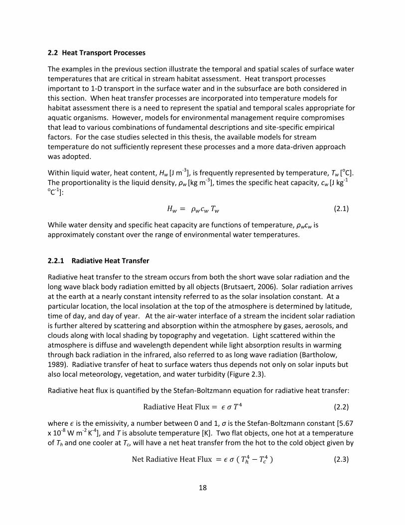
Radiative heat flux is quantified by the Stefan-Boltzmann equation for radiative heat transfer:

Radiative Heat Flux = 𝜖 𝜎 𝑇4 (2.2)

where 𝜖 is the emissivity, a number between 0 and 1, σ is the Stefan-Boltzmann constant [5.67 x 10-8 W m-2 K-4], and T is absolute temperature [K]. Two flat objects, one hot at a temperature of Th and one cooler at Tc, will have a net heat transfer from the hot to the cold object given by

Net Radiative Heat Flux = 𝜖 𝜎 ( 𝑇ℎ4 − 𝑇𝑐

4 ) (2.3)

19

When two environmental media have similar environmental temperatures, such as soil and vegetation, the net radiative heat flux is minor compared to sensible and latent heat flux discussed next. Derivations and descriptions of various empirical formulas to calculate the radiative heat transfer at the air-water interface of a stream are found in Bartholow (1989), Sinokrot and Stefan (1993), and Herbert (2011).

Figure 2.3: Environmental factors influencing the amount of radiative heat transport to the stream. Figure adapted from Bartholow (1989).

2.2.2 Sensible Heat Transfer

Fourier’s Law for diffusive heat transfer represents heat flux within a solid object as proportional to thermal gradient with the proportionality given by a thermal diffusivity

𝐹𝑄 = − 𝜅 𝑑 (𝜌𝑤 𝑐𝑤𝑇)

𝑑𝑥 = −𝜌𝑤 𝑐𝑤 𝜅

𝑑 𝑇

𝑑𝑥 (2.4)

20

where the heat flux, FQ, has the units [J m-2 s-1], κ is the thermal diffusivity [m2 s-1], and frequently the variables ρw cw κ are combined into a single term called the thermal conductivity [J m-1 s-1 K-1]. Heat transfer at environmental interfaces such as the air – water interface cannot directly apply Fourier’s Law because the air and water fluid phases are not stagnant, but have advective flows established by external forcing as well as convective mixing induced by thermal instabilities. Sensible heat flux under these conditions is driven by the difference in temperature of the water and the air with the proportionality factor being a heat transfer coefficient, φs:

𝐹𝑄 = 𝜑𝑠(𝑇𝑤 − 𝑇𝑎 ) (2.5)

where Tw represents the bulk water temperature near the air – water interface and Ta is the bulk air temperature near the air – water interface. The heat transfer coefficient is a function of water and air velocities that locally determine mixing near the interface.

2.2.3 Latent Heat Transfer

Liquid water evaporation requires latent heat to convert the water to a vapor state at a constant temperature. Water evaporation therefore has the potential to lower liquid water temperatures even when the air is warm. Latent heat transfer is proportional to the water evaporation rate expressed as:

𝐹𝑒 = 𝜌𝑤𝐿𝑒𝐸 (2.6)

where Fe is the latent heat flux [J m-2 s-1], Le is the latent heat of vaporization [J kg-1], and E is the volumetric evaporation flux [m3 m-2 s-1 or m s-1]. The water evaporation rate is represented as a mass transfer coefficient, ke times the vapor pressure driving force:

𝐸 = 𝑘𝑒[𝑃𝑤𝑜(𝑇𝑤) − 𝑃𝑤(𝑇𝑎)] (2.7)

where Pwo(Tw) is the saturation vapor pressure of water at the temperature of the water, Tw,

and Pw(Ta) is the actual partial pressure of water in the air having a temperature Ta. The mass transfer coefficient for water evaporation is dependent on wind speed determined through various empirical functions (Allen, 2008; Wagner et al., 2010; Herbert et al., 2011).

2.2.4 Advective and Diffusive/Dispersive Heat Transfer

Heat transport into a section of stream occurs as water advects downstream and is mixed by diffusive or dispersive processes. The advective heat flux, Fa [J m-2 s-1] is quantified by:

𝐹𝑎 = 𝑈𝜌𝑤𝑐𝑤𝑇𝑤 (2.8)

where U is the mean channel velocity [m s-1].

Heat transfer within solids and stagnant fluids is described by Fourier’s Law (Equation 2.4) based on thermal diffusion. In environmental media, additional diffusion processes arise from

21

turbulence and shear dispersion. The total diffusive and dispersive heat flux is quantified analogously to Fourier’s Law:

𝐹𝑑 = −𝐷𝑑(𝜌𝑤𝑐𝑤𝑇𝑤)

𝑑𝑥 (2.9)

where the diffusive/dispersive heat flux, Fd, has the units [J m-2 s-1], and D is a coefficient to represent heat transport by molecular, turbulent, and shear dispersion processes [m2 s-1]. Molecular transport can dominate within stagnant films at the air-water interface and stably stratified water columns, while turbulence and shear dispersion are dominant within flowing surface waters and hydrodynamic dispersion occurs when heat is advected through porous media.

2.2.5 Flow and Heat Transfer through Porous Media

Water flow and heat transport within the streambed arise from local subsurface (hyporheic) flows and groundwater exchange. Granular media in the streambed is first characterized by porosity, n [unitless]:

𝑛 = 𝑉𝑝𝑜𝑟𝑒𝑠

𝑉𝑡𝑜𝑡𝑎𝑙 (2.10)

which is the ratio of the volume of pore space, Vpores , to the total volume, Vtotal representative of the bulk streambed at a spatial scale much greater than the size of the granular material but less than the scale of bed sediment heterogeneities. Water flow through this pore space advects heat and leads to the retardation in heat transport and dispersion due to heat exchange with the solid materials.

The advection of water through porous media is described by Darcy’s Law:

𝑢𝑤 = −𝐾ℎ𝑑ℎ

𝑑𝑥 (2.11)

where uw is the Darcy approach velocity [m s-1], Kh is the hydraulic conductivity [m s-1], and dh/dx is the hydraulic gradient [m m-1]. The Darcy velocity is the volumetric flow of water per total cross-sectional area for the porous medium. The average pore water velocity is estimated by dividing the Darcy velocity by porosity. The hydraulic conductivity is largely dependent upon the size of the granular media and the viscosity of the fluid.

Molecular diffusion and hydrodynamic dispersion occur during the advection of a dissolved tracer through porous media. Random molecular motions create molecular diffusion, while hydrodynamic dispersion occurs as velocity distributions in subsurface pores cause mixing in the direction of flow (Bear, 1979). This similarity between diffusion and dispersion of a tracer allows formulation of the dispersion similar to Fick’s Law:

𝐹𝑚 = −𝐷ℎ𝑑𝐶

𝑑𝑥 (2.12)

22

where Fm is the hydrodynamic dispersion mass flux [kg m-2 s-1], Dh is a mass hydrodynamic dispersion coefficient [m2 s-1], and dC/dx is the tracer concentration gradient in the direction of flow [kg m-4]. The dispersion coefficient quantifies the net effect of both molecular diffusion and hydrodynamic dispersion for tracers in porous media and is calculated from:

𝐷ℎ = 𝐷𝑚 + 𝜆𝐿|𝑢𝑤| (2.13)

where Dm is the molecular diffusion coefficient corrected for porosity and tortuosity [m2 s-1], λL is the hydrodynamic dispersivity [m], and uw is the Darcy velocity [m s-1]. The hydrodynamic dispersivity is scale dependent due to the scale dependence of heterogeneities in the porous network (Neuman, 1990).

Heat transport through porous media by advection and dispersion is calculated from a heat budget for an incremental volume of the porous media.

𝐻𝑎𝑑𝑣𝑒𝑐𝑡,𝑖𝑛 + 𝐻𝑑𝑖𝑠𝑝,𝑖𝑛 = 𝐻𝑎𝑑𝑣𝑒𝑐𝑡,𝑜𝑢𝑡 + 𝐻𝑑𝑖𝑠𝑝,𝑜𝑢𝑡 + ∆𝐻𝑤 + ∆𝐻𝑠 (2.14)

where Hadvect,in is the incoming heat from advection , Hdisp,in is the incoming heat from dispersion, Hadvect,out is the outgoing heat from advection, Hdisp,out is the outgoing heat from dispersion, ΔHw is the change in heat in the pore fluid in the incremental volume, and ΔHs is the change in heat in the solid phase in the incremental volume. Equation 2.14 can be expanded and rewritten as:

𝑢𝑤∆𝑦∆𝑧(𝜌𝑤𝑐𝑤𝑇𝑤)𝑥∆𝑡 + 𝐹𝐻,𝑥∆𝑦∆𝑧∆𝑡 = 𝑢𝑤∆𝑦∆𝑧(𝜌𝑤𝑐𝑤𝑇𝑤)𝑥+∆𝑥∆𝑡

+𝐹𝐻,𝑥+∆𝑥∆𝑦∆𝑧∆𝑡 + 𝑛∆(𝜌𝑊𝑐𝑤𝑇𝑤)∆𝑥∆𝑦∆𝑧 + (1 − 𝑛)∆(𝜌𝑠𝑐𝑠𝑇𝑠)∆𝑥∆𝑦∆𝑧 (2.15)

where uw is the Darcy approach velocity, Δx, Δy, and Δz are incremental distances in the x-, y-, and z-direction [m], Δt is a small increment of time [s], FH is the thermal dispersive flux in porous media [J m-2 s-1], cs is the heat capacity of the solid phase [J kg-1 oC-1], and Ts is the temperature of the solid phase. Equation 2.15 can be rewritten as:

−𝑢𝑤(𝜌𝑤𝑐𝑤𝑇𝑤)𝑥+∆𝑥−(𝜌𝑤𝑐𝑤𝑇𝑤)𝑥

∆𝑥−

(𝐹𝐻,𝑥+∆𝑥−𝐹𝐻,𝑥)

∆𝑥= 𝑛

∆(𝜌𝑊𝑐𝑤𝑇𝑤)

∆𝑡+ (1 − 𝑛)

∆(𝜌𝑠𝑐𝑠𝑇𝑠)

∆𝑡 (2.16)

Assuming that the density and heat capacity of the water and sediment are constant:

−𝑢𝑤𝜌𝑤𝑐𝑤𝜕𝑇𝑤

𝜕𝑥−

𝜕(𝐹𝐻)

𝜕𝑥= 𝑛𝜌𝑊𝑐𝑤

∆𝑇𝑤

∆𝑡+ (1 − 𝑛)𝜌𝑠𝑐𝑠

∆𝑇𝑠

∆𝑡 (2.17)

The thermal dispersive flux in porous media is quantified analogously to a tracer substituting a thermal hydrodynamic dispersion coefficient αT [m

2 s-1] for the mass hydrodynamic dispersion coefficient Dh. The thermal dispersive flux in porous media is modeled by:

𝐹𝐻 = −𝛼𝑇𝑑(𝜌𝑤𝑐𝑤𝑇𝑤)

𝑑𝑥 (2.18)

where the thermal hydrodynamic dispersion coefficient, αT , is the sum of molecular diffusion and hydrodynamic dispersion and is given by:

23

wL

ssww

swT u

cncn

KnnK

)1()(

)1( (2.19)

where Kw is the thermal conductivity of the pore fluid [W m-1 K-1], Ks is the thermal conductivity of the solids [W m-1 K-1] (Anderson, 2005).

The overall one-dimensional advective-diffusive heat transfer equation then becomes

−𝑢𝑤𝜌𝑤𝑐𝑤𝜕𝑇𝑤

𝜕𝑥+

𝜕2(𝛼𝑇𝜌𝑤𝑐𝑤𝑇𝑤)

𝜕𝑥2 = 𝑛𝜌𝑤𝑐𝑤𝜕𝑇𝑤

𝜕𝑡+ (1 − 𝑛)𝜌𝑠𝑐𝑠

𝜕𝑇𝑠

𝜕𝑡 (2.20)

Local equilibrium between the pore fluid and the solid is assumed so Tw = Ts. Additionally, the thermal hydrodynamic dispersion coefficient, density, heat capacity of the fluid and the sediment are assumed to be constant leading to:

−𝑢𝑤𝜌𝑤𝑐𝑤𝜕𝑇

𝜕𝑥+ 𝛼𝑇𝜌𝑤𝑐𝑤

𝜕2𝑇

𝜕𝑥2 = [𝑛𝜌𝑤𝑐𝑤 + (1 − 𝑛)𝜌𝑠𝑐𝑠]𝜕𝑇

𝜕𝑡 (2.21)

Equation 2.21 is rearranged to highlight how heat transport in porous media is retarded by the thermal characteristics of the fluid and solid phases.

−𝑢𝑤

𝑛[1+(1−𝑛

𝑛)(

𝜌𝑠𝑐𝑠𝜌𝑤𝑐𝑤

)]

𝜕𝑇

𝜕𝑥+

𝛼𝑇

𝑛[1+(1−𝑛

𝑛)(

𝜌𝑠𝑐𝑠𝜌𝑤𝑐𝑤

)]

𝜕2𝑇

𝜕𝑥2=

𝜕𝑇

𝜕𝑡 (2.22)

Heat transport will be slower than fluid transport and similarly, dispersion of heat is also reduced because of heat exchange between the pore fluid and the solid phase. This mechanism can be modeled like chemical contaminant retardation during flow and sorption in porous media. In the review article by Rau et al. (2014), heat transport through the subsurface by advection and dispersion is explored in greater depth including how the heat or thermal velocity is retarded compared to the pore water velocity. The retardation of heat transport by subsurface flow through porous sediments is represented by a retardation factor, R, defined as:

𝑅 = 1 + (1−𝑛

𝑛) (

𝜌𝑠𝑐𝑠

𝜌𝑤𝑐𝑤) (2.23)

Equation 2.22 can be rewritten to emphasize how advective and dispersive heat transport is retarded.

−𝑢𝑤

𝑛𝑅

𝜕𝑇

𝜕𝑥+

𝛼𝑇

𝑛𝑅

𝜕2𝑇

𝜕𝑥2=

𝜕𝑇

𝜕𝑡 (2.24)

Both the pore water velocity and the thermal dispersion coefficient are divided by R to account for heat exchange between moving fluid and stationary solid phase. The advective component of heat transport through porous media is related to the Darcy velocity by:

Thermal Velocity = 𝑢𝑇 = 𝑢𝑤

𝑛𝑅 (2.25)

24

Similarly the dispersive component of heat transport in porous media is retarded resulting in a net thermal dispersion coefficient, αD [m2 s-1]:

Net thermal dispersion coefficient = 𝛼𝐷 = 𝛼𝑇

𝑛𝑅 (2.26)

Sediment properties such as hydraulic conductivity and the hydrodynamic dispersivity can vary in space and direction given the complex bedded environment in alluvial channels (Anderson, 2005).

2.2.6 Surface-subsurface exchange in streams

The interaction of surface water and groundwater is an important component of the stream ecosystem and influences the transport of dissolved constituents, biological activity, and thermal conditions in the surface water and groundwater (Hester and Gooseff, 2010). The surface-subsurface exchange between the stream and groundwater occurs through the streambed beneath and adjacent to the stream in the hyporheic zone (Boulton, 2007). The saturated region of the streambed where surface water and deep groundwater mix is generally defined as the hyporheic zone and the interstitial water in this zone possesses characteristics of both surface water and groundwater (White, 1993; Boulton et al., 1998; Hester and Gooseff, 2010). Stanford and Ward (1993) advanced the hyporheic corridor concept which theorized the hyporheic zone existed along the entire length of streams as surface water flows over accumulations of porous alluvium that contain groundwater. Further studies indicated the hyporheic zone is spatially and temporally variable along streams with the extent depending on the hydraulic conductivity in the streambed and fluvial plain, the stream stage, and the geomorphology of the stream channel in the fluvial plain (Boulton et al., 1998; Woessner, 2000).

The transport of surface water through the hyporheic zone along flow paths that return to the surface water is defined as hyporheic flow or exchange. Hyporheic exchange generally occurs when variations in water surface profiles create spatial variations in hydraulic gradients along a stream. Hyporheic exchange downwells when it enters the subsurface and upwells when the hyporheic flow exits the subsurface and re-enters the surface water. Hyporheic flow is distinct from groundwater flow in several different ways (Triska et al., 1989; White, 1993; Harvey et al., 1996; Woessner, 2000) with most researchers agreeing that hyporheic flow is distinguished from groundwater flow by having physical, chemical, and biological properties similar to the surface water (Triska et al., 1989). For this thesis hyporheic exchange has residence times in the subsurface less than a month and groundwater flow has residence times greater than a month. While hyporheic exchange is described as downwelling and upwelling, it is actually a multi-dimensional process with both vertical and horizontal components that occur across a wide range of scales (Poole et al., 2008).

Heat is frequently used as a tracer to investigate the hyporheic exchange in streams (Constantz, 2008), but it is primarily used to quantify the rate of vertical subsurface flow (Hatch et al., 2006; Lautz et al., 2010; Briggs et al., 2012). Stream temperature along the streambed and in the

25

subsurface below the streambed is also frequently measured to quantify the influence of hyporheic exchange on surface water temperature (Arrigoni et al., 2008; Burkholder et al., 2008; Acuña and Tockner, 2009). Ock et al. (2015) documented how gravel augmentation in a sediment-limited system promoted the formation of gravel bars increasing the hyporheic exchange and thermal heterogeneity along the streambed. However, Boulton (2007) noted that a more mechanistic understanding of hyporheic exchange is needed to effectively incorporate it into river restoration activities and restore the ecological benefits of connectivity between surface water and groundwater.

2.2.7 Influence of geomorphology on hyporheic flow

Hyporheic exchange is linked to the geomorphology of a stream because bedforms, channel bends, and topography of the stream and surrounding land all influence the hydraulic head driving hyporheic flow and the formation and shape of hyporheic flow paths (Woessner, 2000; Poole et al., 2008; Boano et al., 2014). At the floodplain scale, variations in the valley, streambed and water surface slope create large scale hydrostatic head differences that drive hyporheic exchange through the alluvial sediment surrounding the stream (Poole et al., 2008; Revelli et al., 2008). At the meander scale, geomorphology influences hyporheic exchange when stream sinuosity forms large hydrostatic pressure gradients across meanders (Boano et al., 2006; Cardenas, 2008). The bathymetry at the pool-riffle scale determines water surface elevations as a function of flow rate (Vaux, 1968; White, 1993; Tonina and Buffington, 2007). Hester and Doyle (2008) and Sawyer et al. (2011) found instream structures like large woody debris alter water surface elevation differences that cause variations in hyporheic exchange. Flow also can change the water surface elevation affecting both the near-bed pressure driving exchange and the surface area available through which exchange can occur (Tonina and Buffington, 2007). At high flows, the water surface elevation variations decrease as bedforms are submerged altering the hydrostatic pressure head driving the hyporheic flow (Tonina and Buffington, 2011). At lower flows, hyporheic flow increases as the emergence of bedforms increases hydrostatic pressure head variations as differences in water surface elevation increase, but very low flows could dewater side channels and shut off hyporheic flow (Boano et al., 2014). Wroblicky et al. (1998) found both the amount and area over which hyporheic flow occurred varied with changes in surface flow by as much as 50%. Local bathymetry and subsurface flow paths are important factors in determining downwelling and upwelling locations, but characterization methods are difficult to scale up to the multiple streambed kilometers important for fisheries habitat assessment.

2.3 Modeling Stream Temperature

Modeling is necessary when there is insufficient data to assess the water temperature conditions in streams or to determine how changes to the stream environment may affect water temperature. Models can utilize available data to estimate existing stream conditions through interpolation and, if the models are process-based, they can provide predictions of water temperature when stream conditions are altered. Many models using a variety of

26

methods have been developed to estimate stream temperature (Caissie, 2006). Either deterministic or statistical modeling methods are used to account for the heat transport processes driving stream temperature. Deterministic models estimate stream temperature by directly calculating a heat budget for sections of one or more streams within a watershed. Deterministic models are useful for quantifying how individual components of the heat budget alter stream temperature, but have the major drawback of requiring significant data inputs which are frequently unavailable. Statistical models identify trends in meteorological and/or stream data to estimate water temperature. Statistical models frequently use air temperature to estimate water temperature because the individual heat budget components influence air and water temperature similarly (Caissie et al., 2001). While statistical models have the advantages of requiring fewer inputs and being relatively simple compared to deterministic models, they cannot be used for cause and effect scenario testing since individual heat budget components are not resolved. Models vary significantly based on what processes are included, how those processes are represented, and the spatial and temporal scales of interest. Models developed for narrow, heavily forested streams frequently emphasize riparian canopy effects on heat transport more than models developed for wide, sparsely vegetated streams.

2.3.1 Surface water temperature modeling

The Stream Network Temperature Model (SNTEMP), MNSTREM, BasinTemp, and a statistical model (Caissie et al., 2001) are several standard models for simulating stream temperature. A brief description of these models is summarized here as an indication of frequent approaches to estimating stream temperature.

SNTEMP is a steady-flow, dynamic one-dimensional deterministic heat transport model that estimates daily mean and maximum stream temperature (Bartholow, 1989). SNTEMP subdivides a stream network into stream reaches with homogeneous properties and then calculates the stream temperature for each reach based on a heat balance. It can estimate stream temperature at time scales from monthly to daily. SNTEMP contains six modules: solar radiation, solar shade, meteorological, heat flux, heat transport, and regression. The solar radiation, solar shade, and meteorological modules provide input to the heat balance module. The heat transport module sums short and long wave radiative heat, latent heat, sensible heat, streambed conduction, advective and diffusive contributions, and stream friction to predict incremental changes in stream temperature. The regression module does parameter fitting for calibration and smooths and/or fills stream temperature data as needed. SNTEMP was primarily designed to predict how alterations in flow regime and canopy cover would affect stream temperature. The Stream Segment Temperature Model (SSTEMP) is a scaled down version of SNTEMP that estimates water temperature for a single stream reach with homogeneous properties for a fixed time increment (e.g. month, week, day) per model run (Bartholow, 2010).

MNSTREM is also a steady-flow, one-dimensional, dynamic temperature model that calculates hourly stream temperature (Sinokrot and Stefan, 1993). MNSTREM is a finite difference, implicit numerical model that solves the one-dimensional heat advection dispersion equation

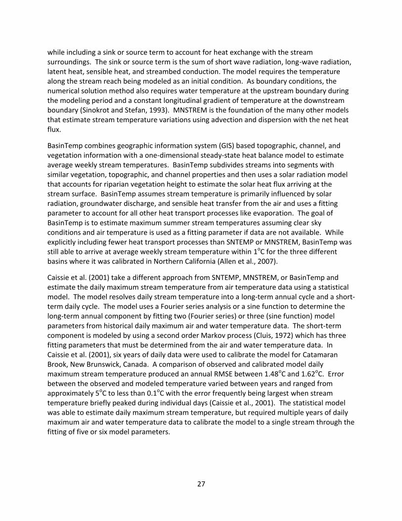
27

while including a sink or source term to account for heat exchange with the stream surroundings. The sink or source term is the sum of short wave radiation, long-wave radiation, latent heat, sensible heat, and streambed conduction. The model requires the temperature along the stream reach being modeled as an initial condition. As boundary conditions, the numerical solution method also requires water temperature at the upstream boundary during the modeling period and a constant longitudinal gradient of temperature at the downstream boundary (Sinokrot and Stefan, 1993). MNSTREM is the foundation of the many other models that estimate stream temperature variations using advection and dispersion with the net heat flux.

BasinTemp combines geographic information system (GIS) based topographic, channel, and vegetation information with a one-dimensional steady-state heat balance model to estimate average weekly stream temperatures. BasinTemp subdivides streams into segments with similar vegetation, topographic, and channel properties and then uses a solar radiation model that accounts for riparian vegetation height to estimate the solar heat flux arriving at the stream surface. BasinTemp assumes stream temperature is primarily influenced by solar radiation, groundwater discharge, and sensible heat transfer from the air and uses a fitting parameter to account for all other heat transport processes like evaporation. The goal of BasinTemp is to estimate maximum summer stream temperatures assuming clear sky conditions and air temperature is used as a fitting parameter if data are not available. While explicitly including fewer heat transport processes than SNTEMP or MNSTREM, BasinTemp was still able to arrive at average weekly stream temperature within 1oC for the three different basins where it was calibrated in Northern California (Allen et al., 2007).

Caissie et al. (2001) take a different approach from SNTEMP, MNSTREM, or BasinTemp and estimate the daily maximum stream temperature from air temperature data using a statistical model. The model resolves daily stream temperature into a long-term annual cycle and a short-term daily cycle. The model uses a Fourier series analysis or a sine function to determine the long-term annual component by fitting two (Fourier series) or three (sine function) model parameters from historical daily maximum air and water temperature data. The short-term component is modeled by using a second order Markov process (Cluis, 1972) which has three fitting parameters that must be determined from the air and water temperature data. In Caissie et al. (2001), six years of daily data were used to calibrate the model for Catamaran Brook, New Brunswick, Canada. A comparison of observed and calibrated model daily maximum stream temperature produced an annual RMSE between 1.48oC and 1.62oC. Error between the observed and modeled temperature varied between years and ranged from approximately 5oC to less than 0.1oC with the error frequently being largest when stream temperature briefly peaked during individual days (Caissie et al., 2001). The statistical model was able to estimate daily maximum stream temperature, but required multiple years of daily maximum air and water temperature data to calibrate the model to a single stream through the fitting of five or six model parameters.

28

2.3.2 Surface – subsurface exchange in stream temperature modeling

Existing surface water temperature models do not resolve groundwater or hyporheic exchange at the scale important to salmonids. Stream temperature models account for the influence of groundwater and hyporheic flow by the inclusion of a reach averaged vertical streambed heat flux in the source or sink term (Herbert et al., 2011). Substantial site specific data are required to include streambed heat flux term into surface water temperature models, yet the models still do not resolve the hyporheic exchange within reaches.

While streambed heat transfer models are available, their application was largely in quantifying streambed recharge rates. Equation 2.22 was solved to determine the velocity of vertical subsurface flow to quantify local groundwater recharge or discharge based on site-specific parameters and subsurface temperature data. Stallman (1965) determined a closed-form analytical solution for 1-D advection dispersion through porous media using a sinusoidal temperature function as the upper boundary condition. Stallman’s model calculates the vertical subsurface water velocity from changes in amplitude and phase shift between subsurface water temperature measured at two depths. Hatch et al. (2006) advanced the model developed Stallman (1965) and refined by Goto et al. (2005) by applying a two-pass forward-backward filter to measured subsurface water temperature to convert measured temperature into a sinusoidal signal of the dominant daily temperature cycle needed as the boundary condition for the analytical solution. The sinusoidal subsurface temperature at two different depths was then used to calculate the vertical subsurface flow velocity from changes in amplitude and changes in phase (Hatch et al., 2006). Another modeling approach uses Dynamic Harmonic Regression (DHR) to isolate the daily cycle in subsurface water temperature data measured at two depths followed by subsurface water velocity determination from the amplitude and phase differences (Keery et al., 2007). Both the Hatch and the Keery modeling approaches for determining the vertical subsurface water velocity were packaged together into Ex-Stream (Swanson and Cardenas, 2011) and VFLUX (Gordon et al., 2012) models. Mechanistic subsurface heat transport models are not currently well integrated into surface water temperature models.

2.4 Statistical Evaluation of Stream Temperature Models

In the development of all models, it is necessary to address model calibration, validation, and the assessment of model predictability using statistical measures of goodness of fit. Bartholow (1989) discusses stream water temperature modeling approaches and the distinction between calibration and validation. In calibration, model parameters are adjusted and model output is compared with observational data to find a combination of model parameters that give the best fit of the model to the observational data. Model validation involves evaluating the calibrated model with data not used in calibration and statistically quantifying how well a model calibrated on one data set can be used in fitting to a similar data set. The validation data set could be observations from a different monitoring period, data available in a similar location, or a combination of both.

29

Statistical evaluation of model fit has been extensively discussed in the hydrologic sciences. In this thesis, I assessed the goodness of fit of a model to data using the Nash-Sutcliffe efficiency, the percent bias, and root mean square error or the root mean square error-observations standard deviation ratio. These three statistical measures are primarily used to evaluate models for surface runoff, streamflow, sediment transport, and nutrients, and were chosen to evaluate how well temperature models performed because of their wide usage and acceptance in hydrology (Moriasi et al., 2007).

The Nash-Sutcliffe efficiency (NSE) calculates variance between the model estimate and the observed data (“noise”) then normalizes it by the variance in the actual observed data (“information”). NSE quantifies how well the observed data agrees with the model estimation and is given by:

𝑁𝑆𝐸 = 1 − [∑ (𝑌𝑖

𝑜𝑏𝑠−𝑌𝑖𝑒𝑠𝑡)

2𝑛𝑖=1

∑ (𝑌𝑖𝑜𝑏𝑠−𝑌𝑚𝑒𝑎𝑛,𝑜𝑏𝑠)

2𝑛𝑖=1

] (2.27)

where Yiobs is the ith observation for the constituent being evaluated, Yi

est is the ith estimated value, Ymean,obs is the mean of the observed data, and n is the total number of observations. NSE ranges from −∞ to 1.0 with NSE equal to 1.0 being a perfect match between the observed data and model estimate (Nash and Sutcliffe, 1970). NSE is sensitive to large differences between the observed and estimated values due to the squared differences, so it is possible to obtain a low NSE for a model if only a few points have very large differences between observed and estimated values. A modified NSE has been suggested by Legates and McCabe (1999) that is less sensitive, but it is not widely used and less accepted as a model performance statistic (Moriasi et al., 2007). The percent bias (PBIAS) quantifies the average tendency of the observed data to be greater than or less than the model estimate with a value of 0 indicating that the model shows no bias. PBIAS is expressed as a percentage of the bias and ranges from −∞ to +∞. Positive values of PBIAS indicate the model underestimates the observations, while negative PBIAS indicates the model provides an overestimation (Gupta et al., 1999). PBIAS is quantified by:

𝑃𝐵𝐼𝐴𝑆 = ∑ (𝑌𝑖

𝑜𝑏𝑠−𝑌𝑖𝑒𝑠𝑡)𝑛

𝑖=1 ∗100

∑ 𝑌𝑖𝑜𝑏𝑠𝑛

𝑖=1

(2.28)

The root mean square error-observations standard deviation ratio (RSR) is the root mean square error (RMSE) between the model estimate and the observed data normalized by the standard deviation of the observed data. RSR ranges from zero to a large positive value with 0 indicating the model estimate perfectly matches the observed data. The RMSE is calculated by:

𝑅𝑀𝑆𝐸 =√∑ (𝑌𝑖

𝑜𝑏𝑠−𝑌𝑖𝑒𝑠𝑡)𝑛

𝑖=1

2

𝑛 (2.29)

where n is the number of observations. The RSR is calculated by:

30

𝑅𝑆𝑅 =𝑅𝑀𝑆𝐸

𝑆𝑇𝐷𝐸𝑉𝑜𝑏𝑠=

√∑ (𝑌𝑖𝑜𝑏𝑠−𝑌𝑖

𝑒𝑠𝑡)𝑛𝑖=1

2

√∑ (𝑌𝑖𝑜𝑏𝑠−𝑌𝑚𝑒𝑎𝑛,𝑜𝑏𝑠)

2𝑛𝑖=1

(2.30)

General model evaluation guidelines recommend using a visual assessment of agreement between the observed data and model estimates along with the NSE, PBIAS, and RSR (Moriasi et al., 2007). Visual agreement is typically the first step in model evaluation with a general visual agreement indicating adequate calibration and validation (Singh et al., 2004). Calculations of NSE, PBIAS, and RMSE or RSR are the next step to evaluate how well a model performs. The range of values of NSE, PBIAS, and RMSE or RSR that determines acceptable model performance is dependent on both the time scale of the model and the constituent being modeled. Typically, model performance decreases for shorter time steps than longer time steps. As the model time step decreases from monthly or weekly to daily, the range of acceptable values for the NSE, PBIAS, and RMSE or RSR will increase (Moriasi et al., 2007). The specific statistics used to evaluate the models developed in the dissertation are explained in the individual chapters.

2.5 Next Steps

This dissertation presents a data driven analysis of stream temperature and develops two separate models that quantify processes critical to assess salmonid survival within coastal California. The watershed-scale temperature model in Chapter 3 and the hyporheic exchange scale temperature model in Chapter 4 utilize relationships and processes that do not appear in existing temperature models. At the watershed scale, the goal is to develop a model that uses readily available data to provide a first order estimate of stream temperature in minimally altered stream environments. At the hyporheic exchange scale, a 1-D subsurface model is formulated for upwelling water temperature that can estimate localized thermal regimes at the streambed. The water temperature models require calibration as do other stream temperature models, and there is an attempt to generalize the modeling approach to permit application at other time periods and nearby locations through a partial validation of the models. The primary contribution of this dissertation is the development of models which are appropriate to the needs of fisheries managers both across entire watersheds and at specific streambed locations.

31

CHAPTER 3

Modeling the spatial distribution of stream water temperatures within watersheds

3.1 Introduction

Habitat assessment requires estimates of environmental conditions within stream networks at locations that cannot be continuously monitored. To assist in this effort techniques are needed to take advantage of available measurements that are distributed spatially over the watershed and temporally. This chapter explores the variation in stream water temperature in three well-instrumented watersheds in coastal California. A model based on readily available air temperature data to represent meteorological forcing and on upstream watershed area can adequately capture stream temperature at points throughout two of the three watersheds.

The chapter is structured with an analysis of each watershed separately followed by cross-watershed comparisons. The watersheds are shown in Figure 3.1 and there is a general decrease in precipitation and increase in summer air temperature as distance from the coast increases. For each watershed there is a description of the local climate, watershed characteristics, land use, and the data utilized in the analysis. Selected data are shown followed by the development of a local stream temperature model. Calibration and verification are undertaken followed by an evaluation of the applicability of a stream temperature model across the three watersheds addressing both temporal and spatial scaling.

3.2 Sonoma Creek Watershed

Sonoma Creek and its tributaries drain a watershed of approximately 430 km2 into the San Pablo Bay, the northern section of the San Francisco Bay. The Sonoma Creek watershed has an elevation range from about 823 m in the headwaters to approximately 2 m above sea level at the Sonoma Creek/Highway 121 bridge. Sonoma Valley has a Mediterranean climate with warm summers and mild wet winters with an average annual rainfall of approximately 890 mm (Leland, 2002). USGS has mapped about 748 km of “blue-line” (first order or greater) streams in the watershed with Sonoma Creek, Schell Creek, and their tributaries forming the drainage network of the valley. Sonoma Creek at its outlet is a fourth order stream running roughly north-south in the center of the watershed for approximately 51 km through the cities of Kenwood, Boyes Hot Springs, Sonoma, and Schellville (SEC, 2007). Land use is a mixture of agricultural, rural residential, protected land, and urban/industrial where the City of Sonoma is the largest city with a population of approximately 11,000. More than 50% of the watershed is forested, but grazing, chaparral, and forested lands are increasingly being converted to vineyards (SEC, 2007). Sonoma Ecology Center and the Southern Sonoma County Resource Conservation District measured the percent total canopy cover along streams in the Sonoma Creek watershed using a spherical densitometer according to the Department of California Fish and Game California Salmonid Stream Habitat Restoration Manual protocols. The mean canopy

32

Figure 3.1: Map of Sonoma Creek, Napa River, and Russian River watersheds.

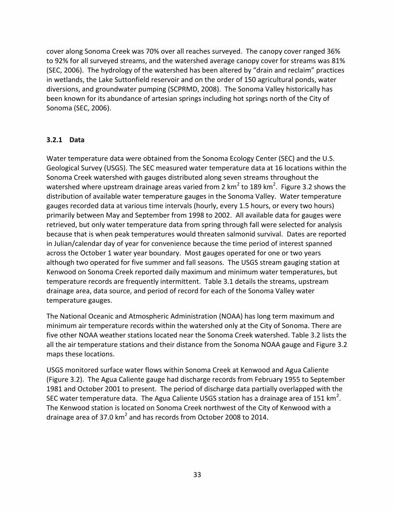
33

cover along Sonoma Creek was 70% over all reaches surveyed. The canopy cover ranged 36% to 92% for all surveyed streams, and the watershed average canopy cover for streams was 81% (SEC, 2006). The hydrology of the watershed has been altered by “drain and reclaim” practices in wetlands, the Lake Suttonfield reservoir and on the order of 150 agricultural ponds, water diversions, and groundwater pumping (SCPRMD, 2008). The Sonoma Valley historically has been known for its abundance of artesian springs including hot springs north of the City of Sonoma (SEC, 2006).

3.2.1 Data

Water temperature data were obtained from the Sonoma Ecology Center (SEC) and the U.S. Geological Survey (USGS). The SEC measured water temperature data at 16 locations within the Sonoma Creek watershed with gauges distributed along seven streams throughout the watershed where upstream drainage areas varied from 2 km2 to 189 km2. Figure 3.2 shows the distribution of available water temperature gauges in the Sonoma Valley. Water temperature gauges recorded data at various time intervals (hourly, every 1.5 hours, or every two hours) primarily between May and September from 1998 to 2002. All available data for gauges were retrieved, but only water temperature data from spring through fall were selected for analysis because that is when peak temperatures would threaten salmonid survival. Dates are reported in Julian/calendar day of year for convenience because the time period of interest spanned across the October 1 water year boundary. Most gauges operated for one or two years although two operated for five summer and fall seasons. The USGS stream gauging station at Kenwood on Sonoma Creek reported daily maximum and minimum water temperatures, but temperature records are frequently intermittent. Table 3.1 details the streams, upstream drainage area, data source, and period of record for each of the Sonoma Valley water temperature gauges.

The National Oceanic and Atmospheric Administration (NOAA) has long term maximum and minimum air temperature records within the watershed only at the City of Sonoma. There are five other NOAA weather stations located near the Sonoma Creek watershed. Table 3.2 lists the all the air temperature stations and their distance from the Sonoma NOAA gauge and Figure 3.2 maps these locations.

USGS monitored surface water flows within Sonoma Creek at Kenwood and Agua Caliente (Figure 3.2). The Agua Caliente gauge had discharge records from February 1955 to September 1981 and October 2001 to present. The period of discharge data partially overlapped with the SEC water temperature data. The Agua Caliente USGS station has a drainage area of 151 km2. The Kenwood station is located on Sonoma Creek northwest of the City of Kenwood with a drainage area of 37.0 km2 and has records from October 2008 to 2014.

34

Figure 3.2: Sonoma Valley, California, showing the locations where discharge, air temperature, and water temperature were measured.

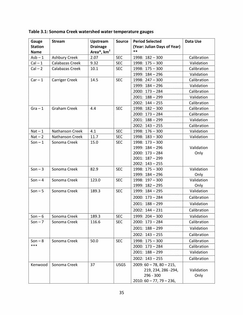
35

Table 3.1: Sonoma Creek watershed water temperature gauges

Gauge Station Name

Stream Upstream Drainage Area*, km2

Source Period Selected (Year: Julian Days of Year) **

Data Use

Asb – 1 Ashbury Creek 2.07 SEC 1998: 182 – 300 Calibration

Cal – 1 Calabazas Creek 9.32 SEC 1998: 175 – 300 Validation

Cal – 2 Calabazas Creek 10.1 SEC 1998: 175 – 300 Calibration

1999: 184 – 296 Validation

Car – 1 Carriger Creek 14.5 SEC 1998: 247 – 300 Calibration

1999: 184 – 296 Validation

2000: 173 – 284 Calibration

2001: 188 – 299 Validation

2002: 144 – 255 Calibration

Gra – 1 Graham Creek 4.4 SEC 1998: 182 – 300 Calibration

2000: 173 – 284 Calibration

2001: 188 – 299 Validation

2002: 143 – 255 Calibration

Nat – 1 Nathanson Creek 4.1 SEC 1998: 176 – 300 Validation

Nat – 2 Nathanson Creek 11.7 SEC 1998: 183 – 300 Validation

Son – 1 Sonoma Creek 15.0 SEC 1998: 173 – 300 1999: 184 – 296 2000: 173 – 284 2001: 187 – 299 2002: 143 – 255

Validation

Only

Son – 3 Sonoma Creek 82.9 SEC 1998: 175 – 300 1999: 184 – 296

Validation Only

Son – 4 Sonoma Creek 123.0 SEC 1998: 197 – 300 1999: 182 – 295

Validation Only

Son – 5 Sonoma Creek

189.3 SEC 1999: 184 – 295 Validation

2000: 173 – 284 Calibration

2001: 188 – 299 Validation

2002: 144 – 231 Calibration

Son – 6 Sonoma Creek 189.3 SEC 1999: 204 – 300 Validation

Son – 7 Sonoma Creek 116.6 SEC 2000: 173 – 284 Calibration

2001: 188 – 299 Validation

2002: 143 – 255 Calibration

Son – 8 ***

Sonoma Creek 50.0 SEC 1998: 175 – 300 Calibration

2000: 173 – 284 Calibration

2001: 188 – 299 Validation

2002: 143 – 255 Calibration

Kenwood Sonoma Creek 37 USGS 2009: 60 – 78, 80 – 215, 219, 234, 286 -294, 296 - 300 2010: 60 – 77, 79 – 236,

Validation

Only

36

238 - 244, 251 - 255, 257 - 266, 291 - 295, 298 – 300 2011: 60 - 167, 169 - 201, 203 - 257, 259 - 286, 288 - 300 2012: 60 – 80, 83 – 116, 118 - 200, 202 - 227, 229 - 241, 243 - 245, 248 - 275, 278 - 300

Stu – 1 Stuart Creek 7.5 SEC 1998: 183 – 300 2001: 222 – 300 2002: 144 – 255

Validation Only

Stu – 2 Stuart Creek 8.3 SEC 2000: 198 – 284 Calibration

* The SEC did not report the upstream drainage for gauge locations, so it was determined using the USGS StreamStats program from gauge latitude and longitude coordinates.

** Period selected restricted to Julian Day of Year 60 to 300. Gaps indicate when no data was available.

*** Son-8 was named Son-2 when data were collected data in 1998.

Table 3.2: Regional air temperature gauges

Weather Station Name

Station ID Number

Coordinates (Lat,Long)

Source Period Selected (Year: Julian Days of Year) *

Distance from Sonoma NOAA Station, km

Sonoma 48351 38.2994, -122.4622

NOAA 1998: 1 – 365 1999: 1 – 365 2000: 1 – 366 2001: 1 – 365 2002: 1 – 365 2009: 2 – 365 2010: 2 – 6, 8 – 13, 15 – 27, 29 – 69, 71 – 76, 78 – 83, 85 – 90, 92 – 97, 99 – 104, 106 – 111, 113 – 118, 120 – 125, 127 – 132, 134 – 139, 141 – 143, 145 – 146, 148 – 153, 155 – 160, 162 – 167, 169 – 174, 176 – 328, 330 – 358, 360 - 365 2011: 2 – 195, 197 – 349, 351 - 365 2012: 1 – 86, 88 – 150, 157 - 326, 328 - 366

0

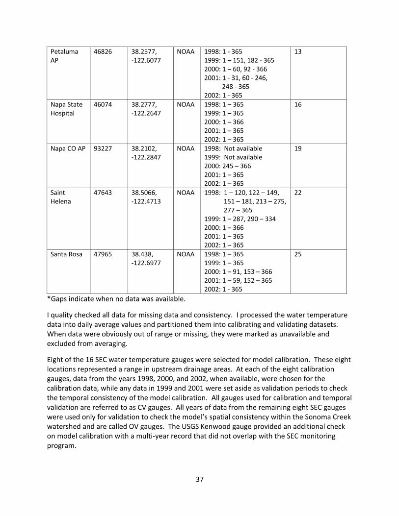
37

Petaluma AP

46826 38.2577, -122.6077

NOAA 1998: 1 - 365 1999: 1 – 151, 182 - 365 2000: 1 – 60, 92 - 366 2001: 1 - 31, 60 - 246, 248 - 365 2002: 1 - 365

13

Napa State Hospital

46074 38.2777, -122.2647

NOAA 1998: 1 – 365 1999: 1 – 365 2000: 1 – 366 2001: 1 – 365 2002: 1 – 365

16

Napa CO AP 93227 38.2102, -122.2847

NOAA 1998: Not available 1999: Not available 2000: 245 – 366 2001: 1 – 365 2002: 1 – 365

19

Saint Helena

47643 38.5066, -122.4713

NOAA 1998: 1 – 120, 122 – 149, 151 – 181, 213 – 275, 277 – 365 1999: 1 – 287, 290 – 334 2000: 1 – 366 2001: 1 – 365 2002: 1 – 365

22

Santa Rosa 47965 38.438, -122.6977

NOAA 1998: 1 – 365 1999: 1 – 365 2000: 1 – 91, 153 – 366 2001: 1 – 59, 152 – 365 2002: 1 - 365

25

*Gaps indicate when no data was available.

I quality checked all data for missing data and consistency. I processed the water temperature data into daily average values and partitioned them into calibrating and validating datasets. When data were obviously out of range or missing, they were marked as unavailable and excluded from averaging.

Eight of the 16 SEC water temperature gauges were selected for model calibration. These eight locations represented a range in upstream drainage areas. At each of the eight calibration gauges, data from the years 1998, 2000, and 2002, when available, were chosen for the calibration data, while any data in 1999 and 2001 were set aside as validation periods to check the temporal consistency of the model calibration. All gauges used for calibration and temporal validation are referred to as CV gauges. All years of data from the remaining eight SEC gauges were used only for validation to check the model’s spatial consistency within the Sonoma Creek watershed and are called OV gauges. The USGS Kenwood gauge provided an additional check on model calibration with a multi-year record that did not overlap with the SEC monitoring program.

38

3.2.2 Overview of Sonoma Data

Since air temperatures were available only at the City of Sonoma within the Sonoma Creek watershed, air temperatures from the five weather stations surrounding the Sonoma Valley were utilized to determine air temperature spatial variability. The daily average air temperatures at each of the five surrounding gauges are plotted in Figure 3.3 against the daily average air temperatures at the Sonoma NOAA gauge for 2002. The air temperatures at Napa County Airport and Petaluma Airport are generally cooler in the summer than the City of Sonoma reflecting their locations nearer to San Pablo Bay. The City of Sonoma air temperatures are generally similar to the inland Napa River drainage basin air temperatures at Saint Helena and the City of Napa (Figure 3.4). In the warmer months, Santa Rosa has more variability in air temperatures probably reflecting the more frequent influence of onshore marine air flows. This comparison suggests that the Sonoma air temperatures provide a reasonable approximation to air temperature within the Sonoma Valley over a spatial distance of 37 km.

Figure 3.3: Variability in the air temperatures near the City of Sonoma.

5 10 15 20 25 305

10

15

20

25

30

Sonoma Air Temperature, oC

Reg

ion

al A

ir T

em

pera

ture

, oC

2002

Petaluma AP

Napa

Napa CO AP

Saint Helena

Santa Rosa

1:1 line

39

Figure 3.4: Air temperature at the Sonoma NOAA gauge was consistent with data from NOAA gauges spanning the north-south axis of the Napa Valley at Saint Helena and Napa.

Stream flow in Sonoma Creek was analyzed at the Agua Caliente and Kenwood USGS gauges from 2003 to 2012 to determine similarities in summer stream flow within the watershed. Daily flow data from 2003 to 2012 at the USGS Agua Caliente gauge were normalized by the upstream drainage area and plotted for the late spring through early fall period in Figure 3.5. While the summer flows varied annually, the exponential decrease is typical when groundwater release dominates stream flow (Tallaksen, 1995). Figure 3.6 shows that normalized Kenwood flows are consistent with the Aqua Caliente gauge. Reported flows from the Kenwood gauge are compromised when the normalized flow drops below 10-2 mm/day (or when the flow drops below approximately 10-1 cfs). The similarity of the recession curves at Kenwood and Agua Caliente suggest that summer baseflow at other locations within Sonoma Creek, Qi, can be estimated by:

𝑄𝑖 = 𝑄𝐴𝐶 𝐴𝑖

𝐴𝐴𝐶 (3.1)

where QAC is the flow at Agua Caliente, Ai is the upstream drainage area at the location for which flow is being determined, AAC is the upstream drainage area at Agua Caliente.

100 150 200 250 300

10

15

20

25

Day of Year

Avera

ge D

aily A

ir T

em

pera

ture

, oC

2002

Sonoma

Napa

Saint Helena

40

Figure 3.5: Flow per area at Agua Caliente on Sonoma Creek consistently had an exponential decrease during the summer.

Figure 3.6: Normalized flow recession curves for Kenwood and Agua Caliente on Sonoma Creek during the summer of 2012.

140 160 180 200 220 240

10-3

10-2

10-1

100

Day of Year

Flo

w p

er

are

a, m

m/d

ay

2003

2004

2005

2006

2007

2008

2009

2010

2011

2012

160 180 200 220 240 260

10-3

10-2

10-1

100

Day of Year

Flo

w p

er

are

a, m

m/d

ay

2012

Kenwood

Agua Caliente

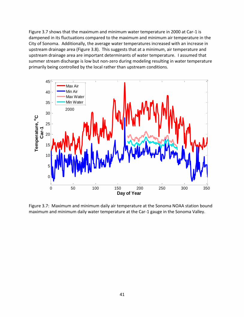
41

Figure 3.7 shows that the maximum and minimum water temperature in 2000 at Car-1 is dampened in its fluctuations compared to the maximum and minimum air temperature in the City of Sonoma. Additionally, the average water temperatures increased with an increase in upstream drainage area (Figure 3.8). This suggests that at a minimum, air temperature and upstream drainage area are important determinants of water temperature. I assumed that summer stream discharge is low but non-zero during modeling resulting in water temperature primarily being controlled by the local rather than upstream conditions.

Figure 3.7: Maximum and minimum daily air temperature at the Sonoma NOAA station bound maximum and minimum daily water temperature at the Car-1 gauge in the Sonoma Valley.

0 50 100 150 200 250 300 350

0

5

10

15

20

25

30

35

40

45

Day of Year

Tem

pera

ture

, oC

Car-

1

2000

Max Air

Min Air

Max Water

Min Water

42

Figure 3.8: Comparison of daily maximum and minimum regional air temperature from the NOAA Sonoma gauge with daily average water temperature from four gauges in the Sonoma Creek watershed for 1998.

3.2.3 Modeling of Stream Temperature

The data in the previous section support a model for daily water temperature based on a linear weighted average of the maximum and minimum air temperatures of the current and some number of prior days, N, to be determined by calibration:

𝑇𝑤𝑎𝑡𝑒𝑟,𝑒𝑠𝑡(𝑡𝑖) = 𝜔

𝑁+1∑ 𝑇𝑎𝑖𝑟,𝑚𝑖𝑛(𝑡𝑗) +

(1−𝜔)

𝑁+1∑ 𝑇𝑎𝑖𝑟,𝑚𝑎𝑥(𝑡𝑗)𝑖

𝑗= 𝑖−𝑁𝑖𝑗= 𝑖−𝑁 (3.2)

where Twater, est is the estimated average daily water temperature [oC], N is the number of preceding days used in the moving average, ω is a linear weighting factor for the contribution of minimum air temperature to water temperature, and Tair, min and Tair, max are the minimum and maximum daily air temperatures [oC].

Calibration

The number of preceding days in the moving average, N, and value of the weighting factor for each gauge, ω, are determined by calibrating the model with air and water temperature data. Table 3.1 lists the 8 gauges that make up the calibration dataset for the years 1998, 2000 and 2002. Data in 1999 and 2001 were reserved for validating the model performance. The model

43

was calibrated in five steps using the Nash-Sutcliffe efficiency (NSE), the percent bias (PBIAS), and the ratio of root mean square error to the standard deviation of the observations (RSR) to quantify model goodness of fit.

Step 1: The initial weighting factors, ω, for all N from zero to nine are calculated from calibration data by using MATLAB’s built-in function “fminsearch” which uses an unconstrained nonlinear optimization of the derivative of equation 3.2. The ω values differed by approximately 0.01 between years. For each value of N from zero to nine, there is a set of ω values for each CV gauge (Figure 3.9). There is limited scatter in ω values as N changes from 0 to 9.

Step 2: The weighting factor, ω, for each calibration data set and N is correlated to the upstream drainage area. The optimum value of ω decreases as the drainage area increases and is fitted to a log function:

𝜔 = 𝑐1𝑙𝑜𝑔10(𝐴𝑢𝑝𝑠𝑡𝑟𝑒𝑎𝑚) + 𝑐2 (3.3)

where c1 and c2 are empirical coefficients that depend upon N values and Aupstream is the drainage area upstream of the gauge [km2].

Step 3: The value of N that optimizes the model goodness of fit is determined by evaluating the NSE, PBIAS, and RSR for each N from 0 to 9. Predicted daily water temperatures are generated using the empirical correlation of ω to watershed area for each N value for the calibration years (Table 3.1). The variations in NSE, PBIAS, and RSR with N for the CV gauges are plotted in Figure 3.10. While PBIAS shows no consistent dependence on N, both NSE and RSR values are optimized for N = 4 so this N value will be used in all further modeling.

Figure 3.9: Variations in minimum air temperature weighting factor, ω, at each gauge for the inclusion of N = 0 to 9 days of prior data in the moving average of air temperatures.

100

101

102

103

0.55

0.60

0.65

0.70

0.75

0.80

0.85

Upstream drainage area, km2

N = 0

N = 1

N = 2

N = 3

N = 4

N = 5

N = 6

N = 7

N = 8

N = 9

44

Figure 3.10: Variations in NSE, PBIAS, and RSR with N, the number of preceding days in the moving average air temperature for all CV gauge data.

Step 4: With N = 4 fixed, the optimum relationships between ω and upstream drainage area was recalculated. Instead of using “fminsearch,” the optimum ω value was determined for each gauge by calculating the NSE, PBIAS, and RSR statics for a range of ω values and selecting the ω value that best optimized all three statics. The optimum ω values are plotted in Figure 3.11 against the upstream drainage area. Optimized ω values determined using the NSE, PBIAS, and RSR were within 0.01 of the values determined by “fminsearch” in Step 1.

0 2 4 6 8-2.5

-2

-1.5

-1

-0.5

0

0.5

1

N, Number of Preceding Days in Moving Average

NS

E

Asb-1

Cal-2

Car-1

Gra-1

Son-5

Son-7

Son-8

Stu-2

0 2 4 6 8-10

-8

-6

-4

-2

0

2

4

N, Number of Preceding Days in Moving Average

PB

IAS

, %

0 2 4 6 80.5

1

1.5

2

N, Number of Preceding Days in Moving Average

RS

R

45

Figure 3.11: Optimum ω value for each CV gauge for N = 4 in Sonoma Creek watershed.

Step 5: A final correlation of optimal ω values to watershed area is determined and becomes:

𝜔 = −0.108 𝑙𝑜𝑔10(𝐴𝑢𝑝𝑠𝑡𝑟𝑒𝑎𝑚) + 0.84 (3.4)

where drainage area is in km2. Equations 3.2 with N = 4 and 3.4 represent the calibrated model to estimate the daily average water temperature for gauges along streams in the Sonoma Creek watershed.

The five step iterative optimization process was done to ensure the model had the best goodness of fit, but comparisons of NSE, PBIAS, and RSR statistics between the initial and final calibration indicate some steps are optional. Table 3.3 summarizes the differences between the initial goodness of fit statistics at the end of Step 3 for N = 4 and the final statistics at the end of Step 5. The gauges show no significant difference between initial and final goodness of fit. This indicates the MATLAB built-in function “fminsearch” sufficiently optimizes ω so Steps 4 and 5 are unnecessary.

100

101

102

103

0.55

0.60

0.65

0.70

0.75

0.80

0.85

Upstream Drainage Area, km2

Asb-1

Cal-2

Car-1

Gra-1

Son-5

Son-7

Son-8

Stu-2

Calibration Equation

46

Table 3.3: Comparison of initial and final CV gauge error statistics

Gauge NSE PBIAS, % RSR

Initial Calib Final Calib Initial Calib Final Calib Initial Calib Final Calib

Asb-1 0.36 0.34 2.09 2.53 0.80 0.81

Cal-2 0.68 0.68 0.54 0.46 0.57 0.57

Car-1 0.43 0.43 1.54 1.36 0.76 0.75

Gra-1 0.41 0.41 0.10 0.29 0.77 0.77

Son-5 -0.54 -0.46 2.99 2.17 1.24 1.21

Son-7 -0.13 -0.18 -1.79 -2.55 1.06 1.09

Son-8 -1.76 -1.96 -7.39 -7.96 1.66 1.72

Stu-2 -0.14 -0.15 -4.81 -4.83 1.07 1.07

Two gauges bound the best (Cal-2) and poorest (Son-8) overall model performance based on the NSE, PBIAS, and RSR measures. The model performance at Cal-2 represents the best fit of the CV gauges. The modeled and observed water temperatures in 1998 at Cal-2 are plotted against time in Figure 3.12 showing water temperature variations were well replicated by the model, although there were limitations in the model performance at all the CV gauges. First, the model tended to under-predict water temperature during cool conditions. Second, the model over-predicted water temperature during the four high-temperature events depicted in Figure 3.12. In a study of data from 584 stream temperature gauges across the USA, Mohseni and Stefan (1999) observed the rate of increase in water temperature declined at high air temperatures, and they proposed that increased evaporative cooling at high air temperatures reduced the peak water temperature in streams. I speculate that the same explanation holds in this watershed since the model tended to over-predict water temperature at many CV gauges during heat waves because the model does not consider evaporative cooling. Third, the modeled local maxima and minima had a tendency to occur after the observed water temperature local maxima and minima by 1 - 2 days. This delay in the water temperature model’s response to extremes in air temperature is believed to be a consequence of the thermal mass of the water in stream pools buffering temperature change and the preceding day moving average of the air temperature. During low-flow summer conditions, streams are primarily small flows of water between large stream pools. The thermal mass of the water in the pools stores and releases heat over several days buffering temperature changes in the stream. The N preceding day moving average air temperature usually accounted for this buffering affect, but the slower change in heat in pools produced a lag between modeled and observed water temperature when water temperature peaked. The number of days in the preceding day moving average attempts to represent the average residence time of the thermal mass in pools.

47

Figure 3.12: Model estimated water temperature data compared with the observed water temperature data at the Cal-2 gauge in Sonoma Creek watershed for 1998.

Figure 3.13 plots the modeled and observed water temperature for the poorest performing CV gauge (Son-8) against the day of the year in 2000 where the observed water temperature is less than the modeled temperature. While the overall trends in the observed water temperature are replicated, the modeled water temperature at Son-8 over-predicts and lags the observed water temperature significantly more than any other CV gauge. Son-8 is located in a narrow canyon with an upstream alluvial valley where groundwater is probably forced to the surface to flow through the canyon (Figure 3.14). The water temperature record at Son-8 thus has a component associated with a local contribution of cool groundwater that lowers the water temperature compared to the model prediction. The watershed temperature model was not intended to represent local sources of groundwater and such sites might be more readily identified through topographic maps, aerial surveys and field observations. The role of groundwater discharge in modeling is discussed in greater detail in Section 3.4.2, Example 3.

180 200 220 240 260 280 30010

12

14

16

18

20

Day of Year

Wate

r T

em

pera

ture

Cal-

2,

oC

Observed

Modeled

48

Figure 3.13: Comparison of modeled and observed water temperature at Son-8 in 2000

Figure 3.14: The location of Son-8 on a USGS topographic map suggests any upstream groundwater is forced to the surface in the canyon causing localized cooling in the stream temperature (adapted from USGS, Kenwood 2012 7.5’ Quadrangle, U.S. Topo).

180 190 200 210 220 230 240 250 260 270 280

13

14

15

16

17

18

19

20

21

22

Day of Year

Wate

r T

em

pera

ture

So

n-8

, oC

Observed

Modeled

Son-8

49

Validation

The calibrated model was validated first by evaluating the model goodness of fit statistics at the eight SEC locations used for calibration (CV gauges) using data from years not included in the calibration. Next, the model was validated by analyzing the model goodness of fit statistics for all years of available data at the eight additional SEC locations along with the USGS Kenwood gauge (OV gauges). This approach assessed the temporal consistency of the model calibration and ascertained the model performance at additional locations within the watershed.

Model performance at CV gauges during the validation years, 1999 and 2001, was generally consistent with the model performance during calibration years (Table 3.4). PBIAS was more negative during validation years indicating the model tended to over-predict water temperature in those years. The NSE and RSR remained similar between calibration and validation years indicating the model consistency in estimating water temperature at CV gauges. Annual variations in the model performance were negligible between calibration and validation years (Figure 3.15). All years demonstrated a similar range of scatter between the modeled and observed water temperature. The model goodness of fit was not correlated with the deviation of ω values from the calibration line in Figure 3.11.

Table 3.4: Comparison of model goodness of fit performance between calibration and validation years for Sonoma Creek watershed CV gauges

Gauge NSE PBIAS, % RSR

Calibration Validation Calibration Validation Calibration Validation

Asb-1 0.34 N/A 2.53 N/A 0.81 N/A

Cal-2 0.68 0.39 0.46 -0.4 0.57 0.78

Car-1 0.43 0.58 1.36 -1.1 0.75 0.65

Gra-1 0.41 0.35 0.29 -2.4 0.77 0.80

Son-5 -0.46 0.12 2.17 -3.4 1.21 0.94

Son-7 -0.18 -0.26 -2.55 -10.0 1.09 1.12

Son-8 -1.96 -2.02 -7.96 -14.9 1.72 1.74

Stu-2 -0.15 N/A -4.83 N/A 1.07 N/A

50

Figure 3.15: The model performance at CV gauges was consistent in both calibration and validation periods at Car-1 in Sonoma Creek watershed.

The eight additional SEC gauges and the Kenwood USGS gauge composing the OV gauges dataset within the Sonoma Creek watershed were used to validate the application of the model to nearby creeks within the watershed. Daily average water temperature was modeled for all nine OV gauges and the NSE, PBIAS, and RSR statistical measures were calculated (Table 3.5).

Model goodness of fit at the OV gauges was comparable or better than the goodness of fit for the CV gauges. NSE values at OV gauges were consistently higher than CV gauge NSE values with only one OV gauge (Son-1) having NSE below zero. The range of PBIAS values for OV gauges were consistent with those for the CV gauges and did not show a significant improvement over the calibration model performance. RSR values were generally within a few percent of zero for validation which was better than the CV gauges. Comparisons of modeled and observed water temperature at Stu-1 in 1998 in Figure 3.16(a) showed that the model primarily over-predicted water temperature during short duration heat waves similar to what was observed at CV gauges. OV gauges had no year to year variability in modeled temperature

51

(Figure 3.16(b)). The variability in the spread of data about the 1:1 line is because the period of record for each year was different. Model performance for the Kenwood gauge over the period 2009 to 2012 was similar to model estimates for SEC OV gauges during the period 1998 to 2002. The consistency of the model performance at CV and OV gauges indicates that Equation 3.4 is valid throughout the Sonoma Creek watershed.

Figure 3.16: (a) Model estimated water temperature data compared with the observed water temperature data at the Stu-1 OV gauge for 1998 in Sonoma Creek watershed. (b) Variability in model performance among years was negligible at Stu-1.

200 220 240 260 280 300

12

14

16

18

20

Day of Year

Wa

ter

Te

mp

era

ture

Stu

-1,

oC

Observed

Modeled

10 12 14 16 18 20 22

10

12

14

16

18

20

22

Observed Water Temperature, oC

Mo

de

led

Wa

ter

Te

mp

era

ture

, oC

1998

2001

2002

1:1 Line

(a)

(b)

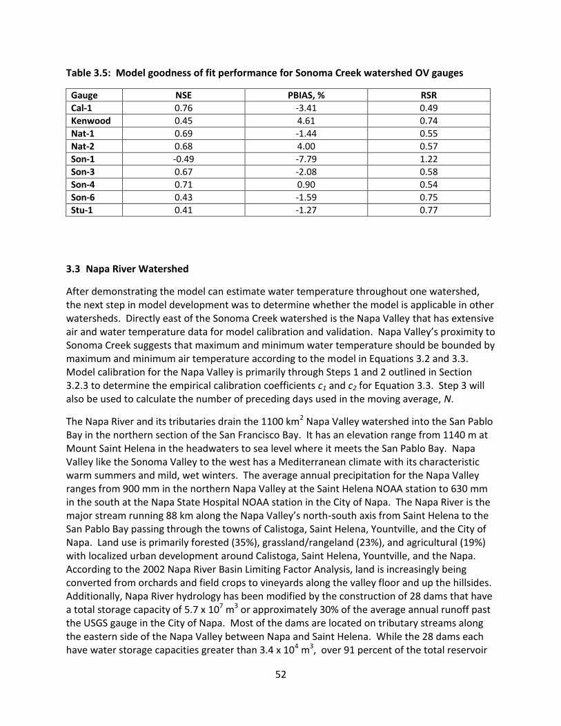
52

Table 3.5: Model goodness of fit performance for Sonoma Creek watershed OV gauges

Gauge NSE PBIAS, % RSR

Cal-1 0.76 -3.41 0.49

Kenwood 0.45 4.61 0.74

Nat-1 0.69 -1.44 0.55

Nat-2 0.68 4.00 0.57

Son-1 -0.49 -7.79 1.22

Son-3 0.67 -2.08 0.58

Son-4 0.71 0.90 0.54

Son-6 0.43 -1.59 0.75

Stu-1 0.41 -1.27 0.77

3.3 Napa River Watershed

After demonstrating the model can estimate water temperature throughout one watershed, the next step in model development was to determine whether the model is applicable in other watersheds. Directly east of the Sonoma Creek watershed is the Napa Valley that has extensive air and water temperature data for model calibration and validation. Napa Valley’s proximity to Sonoma Creek suggests that maximum and minimum water temperature should be bounded by maximum and minimum air temperature according to the model in Equations 3.2 and 3.3. Model calibration for the Napa Valley is primarily through Steps 1 and 2 outlined in Section 3.2.3 to determine the empirical calibration coefficients c1 and c2 for Equation 3.3. Step 3 will also be used to calculate the number of preceding days used in the moving average, N.

The Napa River and its tributaries drain the 1100 km2 Napa Valley watershed into the San Pablo Bay in the northern section of the San Francisco Bay. It has an elevation range from 1140 m at Mount Saint Helena in the headwaters to sea level where it meets the San Pablo Bay. Napa Valley like the Sonoma Valley to the west has a Mediterranean climate with its characteristic warm summers and mild, wet winters. The average annual precipitation for the Napa Valley ranges from 900 mm in the northern Napa Valley at the Saint Helena NOAA station to 630 mm in the south at the Napa State Hospital NOAA station in the City of Napa. The Napa River is the major stream running 88 km along the Napa Valley’s north-south axis from Saint Helena to the San Pablo Bay passing through the towns of Calistoga, Saint Helena, Yountville, and the City of Napa. Land use is primarily forested (35%), grassland/rangeland (23%), and agricultural (19%) with localized urban development around Calistoga, Saint Helena, Yountville, and the Napa. According to the 2002 Napa River Basin Limiting Factor Analysis, land is increasingly being converted from orchards and field crops to vineyards along the valley floor and up the hillsides. Additionally, Napa River hydrology has been modified by the construction of 28 dams that have a total storage capacity of 5.7 x 107 m3 or approximately 30% of the average annual runoff past the USGS gauge in the City of Napa. Most of the dams are located on tributary streams along the eastern side of the Napa Valley between Napa and Saint Helena. While the 28 dams each have water storage capacities greater than 3.4 x 104 m3, over 91 percent of the total reservoir

53

storage in the watershed is contained by the Conn Creek (Lake Hennessey), Rector Creek, Bell Canyon, and Milliken dams (Stillwater Sciences and Dietrich, 2002). Channel modifications, removal of large woody debris, and agricultural encroachment altered the hydrology and morphology of both the Napa River and many of its tributaries leaving only a narrow band of riparian vegetation along streams in the valley floor (Stillwater Sciences and Dietrich, 2002).

3.3.1 Data

Napa Valley water temperature data were obtained from the Berkeley Water Center’s California Datacube which compiled and processed hydrologic data from public agencies. Water temperature data were reported by the USGS and the Napa Resource Conservation District (NRCD) at 22 locations clustered primarily around Saint Helena in the northern Napa Valley and the City of Napa in the southern Napa Valley with drainage areas varying from 2 km2 to 466 km2 (Figure 3.17). NRCD gauges near Saint Helena operated in 2003 and 2004, while NRCD gauges near the City of Napa operated in 2006 and 2007. Table 3.6 details the stream, drainage area, data source, and period selected for each gauge.

NOAA has long term maximum and minimum air temperature records at five locations along the north-south axis of the Napa Valley (Figure 3.17). I obtained the air temperature data from these NOAA stations, and their periods of record are listed in Table 3.7.

USGS has surface water flow data in the Napa River at three locations: Calistoga, Saint Helena, and the City of Napa. The Calistoga USGS gauge station is the farthest upstream with a drainage area of 56.7 km2, but it was only in operation from October 1975 to September 1983. The Saint Helena gauge has a drainage area of 204 km2, while the City of Napa gauge has a drainage area of 564 km2 with both gauges having discharge records from October 1929 to present. Maximum and minimum water temperature data were also collected at Saint Helena from October 1958 to January 1979 and at the City of Napa from October 1976 to 1981. Table 3.8 lists the locations, upstream drainage areas, and periods of records for the USGS gauges on the Napa River.

54

Figure 3.17: Napa Valley, California, showing locations where discharge, air, and water temperature data were collected.

55

Table 3.6: Napa Valley water temperature gauges

Gauge Station Abbreviation

Gauge Station Name

Stream

Upstream Drainage Area*, km2

Source Period Selected (Year: Julian Days of Year)**

Data Use

Big Ranch Big Ranch Road

Unknown 10.4 NRCD 2006: 216 - 300 Validation

2007: 60 - 300 Calibration

Browns 3114 Browns Valley Rd

Browns Creek

10.9 NRCD 2006: 215 - 300 2007: 60 - 300

Validation Only

Crystal crystal springs rd. br.

Bell Creek

15.8 NRCD 2003: 241 – 300 2004: 60 - 300

Discarded (upstream reservoir)

Devlin Devlin Road

Suscol Creek

7.5 NRCD 2006: 216 - 300 2007: 60 - 300

Validation Only

Glass

glass mt. rd. near sewage ponds

Canon Creek

7.5 NRCD 2003: 241 - 300 2004: 60 - 71, 77 – 198

Validation Only

Green Green Valley Road

Spencer Creek

4.9 NRCD 2006: 215 - 300 Validation

2007: 60 - 300 Calibration

Hedgeside Hedgeside Bridge

Milliken Creek

44.8 NRCD 2006: 216 - 300 Validation

2007: 60 - 300 Calibration

Jefferson Jefferson St. Bridge

Napa Creek

39.9 NRCD 2006: 172 - 300 2007: 60 – 98, 103 - 300

Validation Only

Mt. Veeder Mt. Veeder Road

Redwood Creek

7.3 NRCD 2006: 216 - 300 Validation

2007: 60 – 97, 103 - 254

Calibration

Napa-1 pope street bridge

Napa River

180 NRCD 2004: 85 - 253 Validation

Napa-2 Saint Helena

Napa River

204 USGS

1965: 60 - 300 1966: 60 – 151, 181 - 209, 274 - 300 1967: 60 - 300 1968: 60 – 271, 275 - 300 1969: 62 - 300

Validation Only

Napa-3 zinfandel lane br.

Napa River

214 NRCD 2003: 233 - 300 Validation

2004: 60 - 300 Calibration

Napa-4

dwnstm of rutherford x-road

Napa River

246 NRCD 2004: 92 - 250 Validation

56

Napa-5 yountville eco-reserve

Napa River

466 NRCD 2004: 92 - 300 Calibration

Napa-6 City of Napa

Napa River

564 USGS

1978: 61, 67 - 71, 74 - 77, 79, 81 – 92, 94 – 103, 107, 121 – 126, 128 – 137, 139, 141, 143, 145, 147, 151, 153, 157, 159, 161 -165, 167, 169, 172 – 289, 294 -300 1979: 60 – 206, 219 - 273 1980: 80 - 134, 267 - 300 1981: 60 - 292

Validation Only

Redwood Redwood Road pullout

Redwood Creek

25.6 NRCD 2006: 216 - 300 2007: 60 – 300

Validation Only

Shady Brook Shady Brook Lane

Murphy Creek

2.6 NRCD 2006: 215 - 300 Validation

2007: 60 - 300 Calibration

Soda upstream of soda hole

Soda Creek

7.5 NRCD 2004: 155 - 198 Validation

South Terrace

South Terrace Road

Tulucay Creek

24.3 NRCD 2006: 216 - 300 2007: 60 - 300

Validation Only

Spring spring mt. rd.

York Creek

7.3 NRCD 2003: 274 - 300 Validation

2004: 60 - 300 Calibration

State dwnstm of state lane

Rector Creek

29 NRCD 2003: 233 – 300 2004: 60 - 300

Discarded (upstream reservoir)

White whitehall lane near bridge

Bale Slough

1.8 NRCD 2003: 233 - 300 Validation

2004: 85 - 253 Calibration

* When upstream drainage area was not reported for a gauge by the data source, it was determined using the USGS StreamStats program from gauge latitude and longitude coordinates.

** Period selected restricted to Julian Day of Year 60 to 300. Gaps indicate when no data was available.

57

Table 3.7: Napa Valley NOAA air temperature stations

Weather Station Name

Station ID Number

Coordinates (Lat,Long)

Period Selected (Year: Julian Days of Year)*

Calistoga 41312 38.5961, -122.6013

2003: 1 - 46, 48 - 153, 155 - 207, 209 - 258, 260 - 365 2004: 1 - 366 2006: 1 - 365

Saint Helena 47643 38.5066, -122.4713

2003: 1 – 300, 302 - 365 2004: 1 – 47, 55 – 58, 60 – 169, 176, 178 -366 2006: 1 - 365

Yountville 49859 38.395, -122.35667

2003: 1 - 365 2004: 1-93, 95 – 100, 103, 105, 106, 109 – 118, 122 – 187, 189 - 203, 205, 206, 208, 209, 211 - 366 2006: 1 – 31, 60 – 144, 148 - 150, 152 - 365

Napa State Hospital

46074 38.2777, -122.2647

2003: 1 - 365 2004: 1 - 366 2006: 1 - 365 2007: 1 - 365

Napa CO AP 93227 38.2102, -122.2847

2003: 1 – 59, 121 – 151, 182 - 365 2004: 1 - 366 2006: 1 - 365

* Gaps indicate when no data was available.

Table 3.8: Napa Valley USGS discharge gauges

Gauge Station Name

Station ID Number

Stream Upstream Drainage Area, km2

Period Analyzed (Year) Period of Record (Year)

Calistoga 11455900 Napa River

56.7 1980 - 1983 1975 – 1983

Saint Helena

11456000 Napa River

204 1964 - 1970, 1977 - 1983, 2002 - 2009

1929 - current

City of Napa

11458000 Napa River

564 1964 - 1970, 1977 - 1983, 2002 - 2009

1929 - current

Similar to the Sonoma Creek watershed data, I quality checked all Napa Valley data for missing data and consistency and then I partitioned the data into calibrating and validating periods. First, I marked data as unavailable and excluded it from any calculations when the data were obviously out of range or missing. I also discarded two water temperature gauges because they were located downstream of reservoirs where releases likely influenced water temperature. Next, I separated the gauges into two groups: calibration and temporal validation (CV) gauges or only validation (OV) gauges. CV gauges were used to calibrate the model and to validate that the calibration was accurate at those gauge locations over time. OV gauges were used to

58

validate the model spatially and over time at locations not included in the calibration. I selected 10 water temperature gauges representing a range in upstream drainage areas as the CV gauges from the 20 remaining gauges. I randomly selected 2004 and 2007 for the calibration dataset at the 10 CV gauges from the four years of data in the 2000s with a good spatial distribution of data throughout the Napa Valley, while data from 1965 - 1969, 1978 - 1981, 2003, and 2006 were set aside for validation at the CV gauges. Water temperature data existed at the USGS gauges between 1958 and 1993, but the data were frequently discontinuous so USGS gauge data were reserved to validate the model outside of the calibration period. The remaining ten gauges were grouped as the OV gauges and all data at those locations were used only for validation to check the model’s spatial consistency. Table 3.6 details the specific gauges and years used for the calibration and validation datasets.

3.3.2 Overview of Napa Valley Data

Daily average air temperature at the Napa State Hospital weather station was plotted against the daily average air temperature at the other four Napa Valley stations to confirm air temperature was regionally consistent throughout the Napa Valley (Figure 3.18). Similar to the Sonoma Creek air temperature analysis, air temperatures at the Napa Airport were generally cooler than more inland locations during the summer reflecting the Napa Airport’s proximity to the San Pablo Bay. There was a general similarity between air temperatures from Calistoga south to the Napa State Hospital station in the City of Napa. This comparison indicates that the air temperature along the Napa Valley would be equally well represented by data from the Calistoga, St. Helena, Yountville, or Napa State Hospital air temperature gauges. The Napa State Hospital station was chosen as the primary source of air temperature data for the model because the data records are the most complete.

59

Figure 3.18: Daily average air temperature at gauges in the Napa Valley region compared to the daily average air temperature at the Napa State Hospital gauge for 2003.

Summer stream flows in the Napa River at the Calistoga, Saint Helena, and City of Napa USGS gauges were dominated by baseflow. Daily flows were normalized by upstream drainage area, and the data were plotted in Figure 3.19 for 1983. Summer flow recession curves at Saint Helena and the City of Napa have an exponential decrease consistent with baseflow dominated by groundwater releases (Tallaksen, 1995). However, normalized flow only scaled with area between Saint Helena and Napa. Normalized flow at Calistoga consistently receded faster than the other two gauges. Summer baseflow in streams in the Napa Valley can be approximated by:

𝑄𝑖 = 𝑄𝑁𝑃 𝐴𝑖

𝐴𝑁𝑃 (3.5)

where QNP is the flow at the City of Napa, Ai is the upstream drainage area at the location for which flow is being determined, ANP is the upstream drainage area at the City of Napa.

Similar to Sonoma Creek, the average water temperatures recorded in the Napa Valley were bounded by daily air temperature extremes and dependent upon upstream drainage area (Figure 3.20).

5 10 15 20 25 305

10

15

20

25

30

Napa State Hospital Air Temperature, oC

Reg

ion

al A

ir T

em

pera

ture

, oC

2003

Calistoga

Saint Helena

Yountville

Napa AP

1:1 line

60

Figure 3.19: Summer flows normalized by watershed area for the Napa River at Calistoga, Saint Helena, and the City of Napa.

Figure 3.20: The daily average water temperature at gauges in the Napa Valley is bounded by the maximum and minimum regional air temperature, and water temperature increased as the upstream drainage area increased.

140 160 180 200 220 240 260

10-2

10-1

Day of Year

Flo

w p

er

are

a, m

m/d

ay

1983

Calistoga

Saint Helena

Napa

61

3.3.3 Modeling of Stream Temperature in Napa Valley

Water temperatures in Napa Valley streams were modeled using Equation 3.2, a linear weighted average of the maximum and minimum air temperatures of the current and N prior days.

Calibration

The value of the weighting factor for each gauge, ω, and the number of preceding days in the moving average, N, were determined by calibrating the model with air and water temperature data using Steps 1 through 3 outlined in Section 3.2.3. Table 3.6 details the gauges and years used in the calibration and validation. The optimum ω values for all N from 0 to 9 were calculated using “fminsearch,” then these ω values were correlated with upstream drainage area through Equation 3.3. Daily water temperatures were modeled using the empirical correlation of ω to watershed area for each N value for the calibration years. The NSE, PBIAS, and RSR for each N from 0 to 9 were calculated for all the CV gauges and were plotted in Figure 3.21. As observed for the Sonoma Creek watershed, PBIAS in the Napa Valley showed no consistent dependence on N. Both NSE and RSR values were optimized for N = 4 so this N value was used in all further modeling of water temperature in the Napa Valley. The calibration function to determine the optimum ω values for gauges is:

𝜔 = −0.106 𝑙𝑜𝑔10(𝐴𝑢𝑝𝑠𝑡𝑟𝑒𝑎𝑚) + 0.77 (3.6)

where the upstream drainage area is in km2. Equation 3.2 with N = 4 and equation 3.6 represent the calibrated model to estimate the daily average water temperature for streams in Napa Valley.

62

Figure 3.21: Comparison of the NSE, PBIAS, and RSR for Napa Valley calibration gauges indicate that the goodness of fit was optimized for N = 4.

Model goodness of fit performance for the calibration years at Napa Valley CV gauges is summarized in Table 3.9. The model had the poorest performance at the Big Ranch gauge with comparisons of the observed and modeled water temperature in 2007 shown in Figure 3.22. Similar to most CV gauges, the model bias at Big Ranch shifted noticeably from under-predicting prior to DOY 210 to being unbiased after that day. There is additional discussion of the shift in model bias later in this section.

0 2 4 6 8-0.5

0

0.5

1

N, Number of Preceding Days in Moving Average

NS

E

White

Spring

Napa-3

Napa-5

Big Ranch

Green

Hedgeside

Mt. Veeder

Shady Brook

0 2 4 6 8-10

-8

-6

-4

-2

0

2

4

6

8

10

N, Number of Preceding Days in Moving Average

PB

IAS

, %

0 2 4 6 80.4

0.5

0.6

0.7

0.8

0.9

1

1.1

1.2

1.3

N, Number of Preceding Days in Moving Average

RS

R

63

Figure 3.22: Comparison of modeled and observed water temperature at the Big Ranch gauge in 2007 within the Napa Valley.

Table 3.9: Model goodness of fit performance for the Napa Valley calibration years

Gauge NSE PBIAS, % RSR

Big Ranch -0.16 8.52 1.08

Green 0.49 -0.9 0.72

Hedgeside 0.77 0.69 0.48

Mt. Veeder 0.82 -1.59 0.42

Napa-3 0.49 3.32 0.72

Napa-5 0.06 -3.78 0.97

Shady Brook 0.76 0.78 0.49

Spring 0.32 -8.43 0.82

White 0.54 5.19 0.68

The calibrated model performed well at Mt. Veeder with the largest difference between modeled and observed occurring when the model over-predicted water temperature peaks (Figure 3.23). Similar to other gauges, modeled water temperature peaks occurred 1 – 4 days after the observed. The model bias shifted mid-summer with a positive bias for peak temperatures prior to DOY 200 and a slightly negative bias after DOY 200.

100 150 200 250 300

10

12

14

16

18

20

22

Day of Year

Wate

r T

em

pera

ture

Big

Ran

ch

, oC

Observed

Modeled

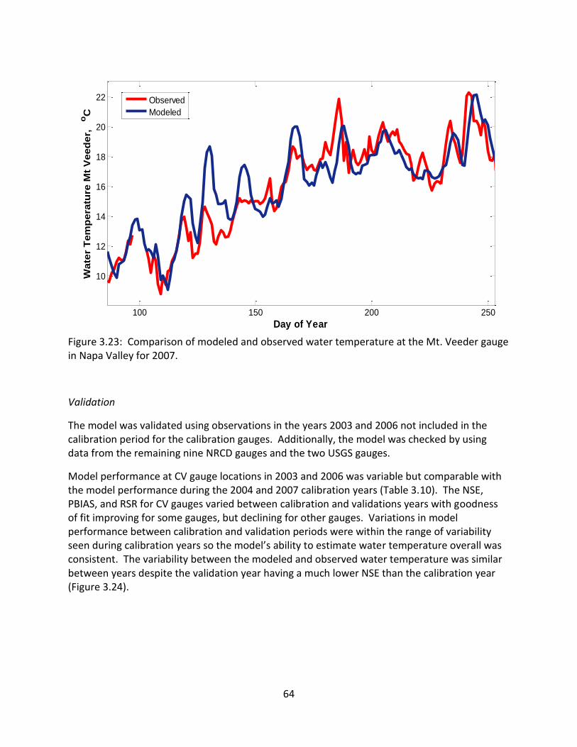
64

Figure 3.23: Comparison of modeled and observed water temperature at the Mt. Veeder gauge in Napa Valley for 2007.

Validation

The model was validated using observations in the years 2003 and 2006 not included in the calibration period for the calibration gauges. Additionally, the model was checked by using data from the remaining nine NRCD gauges and the two USGS gauges.

Model performance at CV gauge locations in 2003 and 2006 was variable but comparable with the model performance during the 2004 and 2007 calibration years (Table 3.10). The NSE, PBIAS, and RSR for CV gauges varied between calibration and validations years with goodness of fit improving for some gauges, but declining for other gauges. Variations in model performance between calibration and validation periods were within the range of variability seen during calibration years so the model’s ability to estimate water temperature overall was consistent. The variability between the modeled and observed water temperature was similar between years despite the validation year having a much lower NSE than the calibration year (Figure 3.24).

100 150 200 250

10

12

14

16

18

20

22

Day of Year

Wate

r T

em

pera

ture

Mt

Veed

er,

oC

Observed

Modeled

65

Table 3.10: Comparison of model goodness of fit performance between calibration and validation years for Napa Valley CV gauges

Gauge NSE PBIAS, % RSR

Calibration Validation Calibration Validation Calibration Validation

Big Ranch -0.16 0.64 8.5 2.2 1.1 0.60

Green 0.49 0.70 -0.90 0.37 0.72 0.55

Hedgeside 0.77 0.58 0.69 -1.7 0.48 0.65

Mt. Veeder 0.82 0.14 -1.6 -8.2 0.42 0.93

Napa-3 0.49 -0.11 3.3 -8 0.72 1.1

Napa-5 0.06 N/A -3.8 N/A 0.97 N/A

Shady Brook

0.76 0.69 0.78 1.9 0.49 0.56

Spring 0.32 -0.17 -8.4 -3.1 0.82 1.1

White 0.54 0.5 5.2 -4.6 0.68 0.71

Figure 3.24: The variability in model performance between calibration and verification years was similar at Napa-3 even if the NSE goodness of fit statistic suggested otherwise.

5 10 15 20 25

5

10

15

20

25

Day of Year

Wa

ter

Te

mp

era

ture

Na

pa

-3,

oC

Calibration (2004) NSE = 0.49

Validation (2003) NSE = - 0.11

1:1 Line

66

Daily average water temperature was estimated for the 9 NRCD and 2 USGS OV gauges and Table 3.11 summarizes the NSE, PBIAS, and RSR statistical measures. Model goodness of fit at validation gauges was comparable to the goodness of fit for CV gauges with three notable exceptions. The Glass, South Terrace and Soda OV gauges all performed poorer than the CV gauges, but the RSR for Glass and South Terrance were still both less than 1.5. The Soda gauge had extremely poor performance with the modeled average water temperature consistently greater than the observed average water temperature (Figure 3.25). Data and historical records suggested significant amounts of cool groundwater were entering the stream near the gauge producing the poor model performance. The average observed water temperature was 14.7oC while the average annual air temperature in the City of Napa was around 15.5oC. The close agreement between water temperature and average annual air temperature further points to groundwater as the source of cool water because the temperature of groundwater is close to the average annual air temperature (USEPA, 1980). Historical records from the mid to late 1800s detail 27 springs in the Soda Springs area that were used to produce more than 3600 bottles of cool mineral water daily (Coodley, 2014). On a USGS topographic map the Soda gauge is around 1 km downstream of a location called Soda Springs which is a plausible source of cool groundwater. The influence of localized groundwater discharge in altering model performance is discussed in greater detail in Section 3.4.2, Example 3.

Figure 3.25: Comparison of observed and modeled water temperature at the Soda OV gauge in Napa Valley.

150 160 170 180 190 200

12

13

14

15

16

17

18

19

20

Day of Year

Wate

r T

em

pera

ture

So

da,

oC

Observed Avg

Observed Max

Observed Min

Modeled Avg

67

Table 3.11: Model goodness of fit performance for Napa Valley OV gauges Gauge NSE PBIAS, % RSR

Browns 0.73 -1.56 0.52

Devlin 0.31 -5.64 0.83

Glass -0.66 3.18 1.29

Jefferson 0.69 -1.37 0.55

Napa-1 0.15 7.22 0.92

Napa-2 0.46 2.78 0.74

Napa-4 0.27 7.96 0.86

Napa-6 0.46 3.96 0.73

Redwood 0.22 -9.5 0.88

Soda -12.98 -15.96 3.74

South Terrace -0.88 -4.86 1.37

A comparison of the observed and modeled water temperature at the Browns gauge in 2007 highlighted the typical performance trends of OV gauges on tributaries of the Napa River (Figure 3.26). The modeled water temperature peaks lagged 1 to 2 days after the observed temperature as seen in the Sonoma Creek watershed. OV gauges also displayed a bias shift mid-summer similar to the CV gauges. The bias changed at Browns around DOY 230 from near zero before to a consistently positive bias afterward. Model performance was consistent at CV and OV gauges during the different years indicating that the calibration function, Equation 3.6, was valid for locations throughout the Napa Valley and for years not utilized in model calibration.

Figure 3.26: Observed and modeled water temperature at the Browns gauge in 2007 had consistent agreement until DOY 230 when the model began to over predict water temperature.

120 140 160 180 200 220 240 260 280

10

12

14

16

18

20

22

Day of Year

Wate

r T

em

pera

ture

Bro

wn

s,

oC

Observed

Modeled

68

Model bias was observed to frequently change around DOY 215 for both CV and OV gauges in the Napa Valley. The shift in bias was consistent from one year to the next, but there was limited spatial consistency in the records. In three of the four years of data for Napa-2 there is a switch from under- to over-prediction of water temperature at about DOY 215. The exception is in 1969 when the bias changed around DOY 150 (Figure 3.27). Model bias shift was quantified by separating the annual data into before and after DOY 215 periods and calculating the PBIAS for each period. Table 3.12 compares the overall value of PBIAS for each year with the two values calculated during each period and suggests general consistency among the years at this location. Flow variations in the Napa River at Napa-2 did not correlate with the timing of PBIAS shifts.

Table 3.12: Annual variation in PBIAS shift at Napa-2

Year* Overall PBIAS, % PBIAS: Before DOY 215, % PBIAS: After DOY 215, %

1965 8.2 13.9 -1.8

1967 4.7 13.4 -10.0

1968 3.0 9.7 -10.5

1969 -3.4 2.4 -13.2

*1966 was excluded because observed water temperature data was sparse

67

Figure 3.27: Model bias consistently changed mid-year at Napa-2 resulting in the model going from under- to over-predicting water temperature.

100 150 200 250 300

10

15

20

25

1965

Day of Year

Wa

ter

Te

mp

era

ture

Nap

a-2

, oC

Observed

Modeled

100 150 200 250 300

10

15

20

25

1966

Day of Year

Wa

ter

Te

mp

era

ture

Nap

a-2

, oC

Observed

Modeled

100 150 200 250 300

10

15

20

25

1968

Day of Year

Wa

ter

Te

mp

era

ture

Nap

a-2

, oC

Observed

Modeled

100 150 200 250 300

10

15

20

25

1969

Day of Year

Wa

ter

Te

mp

era

ture

Nap

a-2

, oC

Observed

Modeled

69

70

There was no consistent spatial pattern in the PBIAS shift. Figure 3.28 plots measured and modeled water temperature for 4 Napa River gauges with upstream drainage area that varied by only a factor of 2.6. While bias shifts occurred around DOY 215 at all the gauges, the magnitude of the bias shift varied between gauges and it did not consistently vary with changes in drainage area. The limited water temperature data for Napa-1 and Napa-4 suggest a larger shift in bias at the upstream Napa-1 than at the downstream Napa-4 after DOY 215. However, the downstream Napa-5 showed a larger bias shift than at the upstream Napa-3. The presence of a PBIAS shift was also spatially variable with not all gauges showing a PBIAS shift. The Shady Brook and Green gauges were in different sub-watersheds and located only 0.8 km apart, but Shady Brook had a negligible PBIAS shift while Green switched from over- to under-predicting water temperature. Table 3.13 summarizes the overall PBIAS, the PBIAS before DOY 215, and the PBIAS after DOY 215 for all gauges and all years of data.

Table 3.13: Comparison of changes in PBIAS before and after DOY 215 for all years with data available

Gauge Overall PBIAS, % PBIAS: Before DOY 215, % PBIAS: After DOY 215, %

Big Ranch 8.5 12.3 0.59

Browns -1.56 -4.10 1.39

Devlin -5.63 -2.86 -8.06

Glass 3.18 6.11 -3.06

Green -0.90 4.11 -10.2

Hedgeside 0.69 3.62 -4.47

Jefferson -1.37 0.75 -3.76

Mt. Veeder -1.6 -2.1 0.08

Napa-1* 7.22 10.68 -3.62

Napa-2 2.78 10.36 -11.58

Napa-3 3.3 5.43 -0.08

Napa-4* 7.96 8.52 6.65

Napa-5 -3.8 2.64 -13.3

Napa-6 3.96 6.50 -0.01

Redwood -9.5 -8.92 -9.93

Shady 0.78 1.08 0.31

South Terrace -4.86 -2.73 -6.72

Spring -8.43 -7.67 -9.54

White 5.19 5.93 3.09

* Data is limited after DOY 215

69

Figure 3.28: Observed and modeled water temperature along the Napa River in 2004.

100 150 200 250 300

10

15

20

25

Day of Year

Wate

r T

em

pera

ture

Nap

a-1

, oC

Observed

Modeled

100 150 200 250 300

10

15

20

25

Day of Year

Wate

r T

em

pera

ture

Nap

a-3

, oC

Observed

Modeled

100 150 200 250 300

10

15

20

25

Day of Year

Wate

r T

em

pera

ture

Nap

a-4

, oC

Observed

Modeled

100 150 200 250 300

10

15

20

25

Day of Year

Wate

r T

em

pera

ture

Nap

a-5

, oC

Observed

Modeled

71

72

3.4 Russian River Watershed

While the Russian River watershed is immediately to the west of the Sonoma watershed, conditions were not suitable for successful water temperature prediction using available air temperature records and watershed area. This section demonstrates water temperature modeling is compromised by the spatial variability in air temperature of a significantly larger watershed, possible geologic controls that influence groundwater contributions, and hydrologic modifications by dams and extractions. Following a brief review of the watershed and hydrologic modifications, data sources are documented, and four examples are presented that demonstrated model applicability as well as limitations in the watershed. The Russian River watershed is a 3800 km2 basin stretching from the inland Redwood and Potter Valleys north of Ukiah, California, south to Healdsburg, California, then sharply turning west to drain into the Pacific Ocean near Jenner, California. The watershed, like Napa and Sonoma, has a Mediterranean climate, but its size and location closer to the Pacific Ocean provides a wide range of climate. Summers in the coastal region extending approximately 16 km inland are dominated by cool marine fog while inland regions are hot and dry with air temperature frequently exceeding 38oC. The average annual precipitation for the Russian River watershed ranges from 560 mm to 2030 mm with the highest precipitation occurring in the coastal mountains and at the higher elevations near Mount Saint Helena on the eastern boundary. The Russian River is the main waterway with a length of 177 km along the axis of the watershed. Land use is primarily open rangeland and agriculture with a trend toward converting historic crop land, rangeland, and forest into vineyards. Other land uses include timber harvesting, gravel mining, rural residential, tourism, urban, and some industrial. Russian River hydrology has been extensively modified by dams and water diversions. There are 509 licensed or permitted small tributary dams, five impoundments on the mainstem Russian River, and two major dams: Coyote Valley and Warm Springs. Coyote Valley Dam was built on the East Fork Russian River near Ukiah with an estimated design storage capacity of 1.1 x 108 m3. Warm Springs Dam was built on Dry Creek, a tributary of the Russian River near Geyserville, with a storage capacity of 4.7 x 108 m3. Both dams alter the flow of the Russian River by releasing water during the summer months with Coyote Valley releasing at least 3.5 m3 s-1 into the Russian River at Ukiah and Warm Springs releasing approximately 2.8 m3 s-1 into the Russian River below Healdsburg (CDFG, 2002). Dam releases also are strong controls on channel geomorphology altering the groundwater levels in adjacent alluvial valleys and potentially affecting tributary stream flow. Walls (2013) investigated how to use aerial imagery to determine intermittency in streams and documented relationships between mainstem flow and the length of wetted channel in tributaries. In addition to dams, numerous water diversions have altered Russian River watershed hydrology with more than 2600 points of diversion in the watershed (Dietch et al., 2009). The Potter Valley Project is the most significant diversion with up to 8.5 m3 s-1 diverted from the Eel River watershed to the north into the East Fork Russian River upstream of Coyote Valley Dam. While the Potter Valley diversion increases flow into the Russian River, localized agricultural diversions decrease flow into the mainstem Russian River and its tributaries causing depressions in baseflow and intermittency (Dietch et

73

al., 2009). These modifications along the mainstem of the Russian River provide examples where assumptions of local, summer water temperature within a natural stream based on air temperature and watershed area are compromised.

3.4.1 Data

Water temperature data were obtained from the Berkeley Water Center’s California Datacube which compiled and processed hydrologic data from the USGS, the Sonoma Ecology Center (SEC), the Mendocino County Water Agency (MCWA), the Mendocino Redwood Company (MRC), and the Forest Science Project (FSP). Daily water temperature records from 1996 to 2010 were available for analysis at 24 locations distributed along the Russian River and its tributaries with drainage areas varying from 2 km2 to 3470 km2 (Figure 3.29). Table 3.14 summarizes the streams, drainage area, data source, and the years available. Air temperature data were obtained from eight NOAA weather stations along the length of the Russian River and its vicinity between 1996 and 2010 (Figure 3.29). Air temperature data were also available from two MCWA water temperature gauges. Table 3.15 lists the stations and their periods of record.

Surface water flow data in the Russian River watershed were available at 30 locations on 16 different waterways. Data from five locations along the East Fork and mainstem Russian River were used to document the effect of releases from Lake Mendocino (Table 3.16).

74

Figure 3.29: Map of the Russian River watershed with air and water temperature gauge locations.

75

Table 3.14: Russian River watershed water temperature gauges

Gauge Station Name

Stream Upstream Drainage Area*, km2

Source Station ID Number

Years Available

Ack-01 Ackerman Creek 13.2 MRC MRC05-T83-04 2003

Ack-02 Ackerman Creek 17.4 MRC MRC05-T83-01 2002, 2004, 2005

Ack-03 Ackerman Creek 36.8 MRC MRC05-T83-03 2002

Ack-04 Ackerman Creek 47.7 MCWA MCWAS-159 1999 – 2003

Dooley-1 Dooley Creek 39.6 MCWA MCWAS-77 1997

Fors-1 Forsythe Creek 38.9 MCWA MCWAS-111 2000 - 2004

Fors-2 Forsythe Creek 41.2 MCWA MCWAS-181b 2001, 2003

Fors-3 Forsythe Creek 78.2 MCWA MCWAS-158 1999, 2000

Freeze-1 Freezeout Creek 2.33 MRC MRC05-T98-20 2004

Freeze-2 Freezeout Creek 3.63 FSPS / MRC

FSPS-2125/ MRC05-T98-04

1996, 1997, 2002, 2003

Gibs-1 Gibson Creek 4.14 MCWA MCWAS-161 1999 - 2004

JackS-1 Jack Smith Creek 8.03 FSPS/ MRC

FSPS-2090/ MRC05-T77-01

1996, 1997, 2002 - 2005

Mill-1 Mill Creek 14.8 MCWA MCWAS-108 2000:

RR01 Upper Russian River

4.92 MCWA MCWAS-120 2000 - 2004

RR-02 Russian River 79.0 MCWA MCWAS-182 2000 - 2003

RR-03

East Fork Russian River

272 USGS 11462000 1990 – 1994

RR-04 East Fork Russian River

272 MCWA MCWAS-72 1997- 2003

RR-05 Russian River 670 MCWA MCWAS-183 2000 - 2004

RR-06 Russian River 1008 USGS 11462500 2001 - 2010

RR-07 Russian River 1260 MCWA MCWAS-75 1999 - 2003

RR-08 Russian River 1303 USGS 11463000 2009 - 2011

RR-09 Russian River 2049 USGS 11463980 2002 - 2011

RR-10 Russian River 2057 USGS 11464000 1995 – 2008

RR-11 Russian River 3466 USGS 11467000 2002 – 2010

* When upstream drainage area was not reported for a gauge by the data gathering entity, it was calculated using the USGS StreamStats program based on gauge latitude and longitude.

76

Table 3.15: Russian River regional air temperature gauges

Weather Station Name

Station ID Number Coordinates (Lat,Long)

Source Years Available

Potter Valley Powerhouse

47109 39.367, -123.133

NOAA 2000 - 2010

RR01 MCWAS-120 39.366, -123.235

MCWA 2000 - 2004

Ukiah 49122 39.150, -123.217

NOAA 1996 - 2010

RR07 MCWAS-75 38.887, -123.053

MCWA 2000, 2002, 2004

Cloverdale 41838 38.800, -123.017

NOAA 1996 - 2010

Healdsburg 43875 38.617, -122.867

NOAA 1996 - 2010

Santa Rosa 47965 38.438, -122.6977

NOAA 1998 - 2004

Graton 43578 38.433, -122.867

NOAA 1996 - 2010

Occidental 46370 38.383, -122.967

NOAA 2000 - 2004

Fort Ross 43191 38.517, -123.250

NOAA 1996 - 2004

Table 3.16: Russian River watershed USGS discharge gauges

Gauge Station Name

Location Station ID Number

Stream Upstream Drainage Area, km2

Years Available

Ukiah Ukiah (upstream of the East Fork Russian River)

11461000 Russian River 259 1911 - 2014

RR-03 Ukiah (downstream of

Coyote Valley Dam on the East Fork Russian River)

11462000 East Fork Russian River

272 1911 - 2011

RR-06 Hopland 11462500 Russian River 1008 1939 - 2014

RR-08 Cloverdale 11463000 Russian River 1303 1951 - 2014

RR-10 Healdsburg 11464000 Russian River 2057 1939 - 2014

77

3.4.2 Water Temperature Modeling in Russian River Watershed

Four locations within the Russian River watershed were selected to demonstrate the application and some limitations of the air temperature based model. These examples illustrate how the model results can be compromised by significant spatial variability in air temperature, groundwater inflows dominated by local geologic conditions, and flow augmentation by reservoir operations. The model could not estimate stream temperature within 2oC, but it was valuable for identifying areas where stream temperature is governed by local groundwater influences and anthropogenic alterations like water diversions. When more accurate stream temperature estimates are required, the collection of the necessary data inputs in those specific reaches and application of a more resolved 1-D reach scale model are reasonable next steps. Example 1: Model applicability

The model is applicable for estimating water temperature when air temperature data are measured coincident with the water temperature data. Water temperature was measured at the RR-10 gauge while air temperature was measured 2.4 km north of the gauge in Healdsburg. General trends in observed and modeled water temperature tended to agree with the largest difference occurring when the model over-predicted water temperature peaks (Figure 3.30). Modeled water temperature also tended to peak 1-2 days after observed water temperature. Model goodness of fit statistics at RR-10 near Healdsburg were comparable to the calibrations in the Sonoma and Napa watersheds with an NSE of 0.75, a PBIAS of 1.3%, and a RSR of 0.50.

Figure 3.30: Comparison of observed and modeled water temperature at RR-10, Russian River.

140 160 180 200 220 240 260

16

18

20

22

24

26

Day of Year

Wate

r T

em

pera

ture

RR

-10,

oC

2002

Observed

Modeled

78

Example 2: Spatial variability in air temperature

There is considerable spatial variability in air temperature within the Russian River watershed due to its proximity to the Pacific Ocean and large size which gives rise to numerous microclimates that range from cool coastal to warm inland environments. The spatial variability in air temperature decreases the model performance if selected air temperature data do not reflect the local environment where water temperatures were measured. The first example above demonstrated that the model performed well at RR-10 because the air temperature data at Healdsburg accurately represented local conditions. To illustrate the effect of alternative choices for air temperature records, data from Ukiah to the north and Graton to the southwest are utilized. Figure 3.31 compares Healdsburg average daily air temperatures observations in Ukiah and Graton in 2000. The air temperature record in Ukiah is comparable to Healdsburg with considerable scatter, while summer temperatures in Graton are cooler with considerable scatter. When the Ukiah and Graton air temperature data were used in the model, the NSEs decreased and the biases increased compared to what was achievable with the Healdsburg air temperature data (Table 3.17).

Figure 3.31: Variability in air temperature between Ukiah, Healdsburg, and Graton in 2000.

10 20 305

10

15

20

25

30

35

Healdsburg Air Temperature, oC

Ukia

h A

ir T

em

pera

ture

, oC

10 20 305

10

15

20

25

30

35

Healdsburg Air Temperature, oC

Gra

ton

Air

Tem

pera

ture

, oC

79

Table 3.17: Variability in model performance with air temperature source at RR-10

Air Temperature Source NSE PBIAS RSR

Healdsburg 0.75 1.3 0.50

Ukiah 0.59 4.5 0.64

Graton 0.56 6.6 0.66

Example 3: Geologic controls on groundwater contribution

The empirical modeling approach used in this chapter was based on the increase in stream temperature with increasing watershed area reflecting less contribution from local groundwater discharges and more opportunities for surface water heating from the atmosphere. Water temperature at two locations in Ackerman Creek provided a good example of how localized cool groundwater contributions can alter the standard pattern of stream temperature. While water temperature normally increases with distance downstream, water temperature was less at Ack-4 than at the Ack-3 gauge located 7 km upstream (Figure 3.32). While Ack-3 is presumed to be the source of flow for Ack-4, a source of cold water must exist between Ack-3 and Ack-4 for the observed water temperature at Ack-4 to be consistently cooler. Ack-4 is immediately downstream of a gap in the surrounding mountain range, and a review of USGS topographic maps suggest that the cold water source is subsurface groundwater forced to the surface by local geologic conditions (Figure 3.33). In the summer when streamflows continue to fall, the increased cooling of Ack-4 compared to Ack-3 suggests an increased contribution of cool groundwater to the overall flow at Ack-4. No stream gauging data are available for these sites.

Figure 3.32: Ackerman Creek is a tributary of the Russian River and Ack-3 had consistently warmer water temperature than Ack-4 about 7 km downstream.

170 180 190 200 210 220 230 240

16

17

18

19

20

21

22

23

Day of Year

Wa

ter

Te

mp

era

ture

, oC

Ack-3

Ack-4

80

Figure 3.33: Geologic conditions may be forcing subsurface groundwater flow upwards into the surface flow in Ackerman Creek upstream of Ack-4 (adapted from USGS, Ukiah and Orr Springs 2015 7.5’ Quadrangle, U.S. Topo).

Stream temperatures at Ack-4 in the Russian River watershed, Son-8 in the Sonoma watershed, and Soda in the Napa watershed are not captured by the watershed model because temperature at these locations is controlled by local geologic conditions that force groundwater to the surface. The model overestimates stream temperature providing a conservative approximation of thermal habitat. When stream temperature data are available at specific locations, comparison between observed and modeled temperatures can highlight the presence of a localized groundwater source that would justify field investigations.

Example 4: Flow augmentation by reservoir operations

The model was developed for assessing the aquatic habitat during flows in the summer and fall critical periods common in Mediterranean climates. During these low flow periods the water

81

temperature depended largely upon local air temperature. However, summer and fall flows in the mainstem of the Russian River below Ukiah are dominated by reservoir releases that far exceed natural flows as illustrated in Figure 3.34. The location of the gauges listed in Figure 3.34 can be found in Figure 3.29. The flow record at Ukiah (West Fork Russian River) shows exponential baseflow recession comparable to other minimally altered flows in coastal California. The flow record at RR-03 immediately downstream of Lake Mendocino on the East Fork of the Russian River shows a near constant flow rate of approximately 5 m3 s-1. The three other flow records from gauges on the mainstem Russian River below its confluence with the East Fork Russian River are dominated by the flow rate from Lake Mendocino seen in the RR-03 flow record.

Reservoir releases substantially alter water temperatures in the East Fork and mainstem Russian River below Ukiah for a substantial distance downstream during the summer and fall (Figure 3.35). At RR-03 on the East Fork of the Russian River located immediately below Lake Mendocino, the water temperature has only a long-term seasonal variation. There is a systematic increase in both mean water temperature and its daily variations downstream of RR-03 on the mainstem Russian River. Similar air temperature data at Ukiah and Healdsburg (Figure 3.31) indicate atmospheric forcing is consistent between RR-03 and RR-10, so the increase in water temperature and greater daily variations is a result of atmospheric heating of the river. The water temperature record at RR-10 near Healdsburg reflects coupling with the air temperature record while the upstream water temperatures are dominated by Lake Mendocino releases. Approximate flow times to the gauge locations from Lake Mendocino were calculated using USGS measurements of depth, width, and flow at Russian River gauging stations (Table 3.18). Travel time estimates indicate reservoir releases influence water temperature in the Russian River during the two-day flow time from Lake Mendocino to RR-07. At RR-10 near Healdsburg, 110 km downstream from Lake Mendocino and a 5-day transit time, there is no influence of reservoir releases based on the seasonal trend with daily variations in water temperature. Reservoir releases of cooler water appear to alter downstream water temperatures for flow times of at least 2 days but less than 5 days on the Russian River. Example 1 demonstrated that the model was able to estimate water temperature at RR-10 near Healdsburg given the 5-day flow time and the limited spatial variability in air temperature between Ukiah and Healdsburg (Figure 3.30).

Table 3.18: Comparison of travel times in the East Fork and mainstem Russian River when flow is 5 m3 s-1

Location Distance (km) Travel time (days)

RR-03 0 0

RR-05 7.5 0.2

RR-06 32 1

RR-07 45 2

RR-10 110 5

82

Figure 3.34: Dry season baseflow recession is observed in the Russian River at Ukiah, but flow augmentation by the releases from the Coyote Valley Dam on the East Fork Russian River (EFRR) dominates downstream gauge

Figure 3.35: Coyote Valley Dam releases from Lake Mendocino alter water temperature in the East Fork Russian River and the mainstem Russian River as far downstream as RR-07.

60 80 100 120 140 160 180 20010

-3

10-2

10-1

100

101

102

Day of Year

Flo

w,

m3/s

2002

Ukiah

RR-03

RR-06

RR-08

RR-10

83

3.5 Comparison Between Watersheds

One of the goals of this work besides demonstrating the application of a water temperature model based on air temperature was to explore the model’s application to ungauged locations. While there was an area dependence to the weighting parameter, ω, the difference between the Sonoma and Napa calibration equations is slight. Figure 3.36 plots the best fit individual ω values and the correlation equation between ω and watershed area for each watershed. In addition the best fit Russian River value of ω at location RR-10 is indicated with a red dot in Figure 3.36, and that fitted value lies within the bounds established for the Sonoma and Napa watersheds. The upstream drainage area at RR-10 is almost 4 times greater than the maximum drainage area in Napa and 11 times greater than the largest Sonoma drainage area. These results suggest that the correlation of ω to drainage area can be extrapolated to nearby basins and beyond the range of upstream drainage areas utilized for calibration in the Sonoma and Napa basins.

Figure 3.36: The calibration equations for the weighting parameter, ω, plotted against the upstream drainage area along with fitted value at Russian River gauge RR-10 near Healdsburg.

100

101

102

103

0.35

0.40

0.45

0.50

0.55

0.60

0.65

0.70

0.75

0.80

0.85

Upstream Drainage Area, km2

Sonoma Optimum

Sonoma Calibration

Napa Optimum

Napa Calibration

RR10 - HealdsburgRR-10

84

3.6 Discussion

A surface water temperature model based on the weighted average of the maximum and minimum air temperature was developed in this chapter. It was built upon the relationship between air and water temperature observed by Mohseni and Stefan (1999) and the recognition that stream temperature increases with distance from the stream headwaters (Sullivan and Dhakal, 2008; Forney et al. 2013). The key contribution of my research was quantitatively relating stream temperature to air temperature through upstream drainage area and the model weighting factor parameter. While the calibration equation to estimate the weighting factor from upstream drainage area is empirically determined, it is physically based on the principal that stream temperature increases with watershed area as the local groundwater contribution decreases and there is greater opportunity for atmospheric heating of the surface water. Relating air and stream temperature through upstream drainage area and the weighting factor enabled the model to estimate daily average stream temperature within 1.5oC most of the time using only air temperature data once the model was calibrated. This also makes the model practical for application in data sparse environments because it has only two calibration parameters, ω and N, which do not require a large dataset for calibration.

The model is an improvement over other approaches to stream temperature modeling across watersheds because the data requirements are minimal. The statistical stream temperature model developed by Caissie et al. (2001) had an accuracy of approximately 1.5oC similar to my weighted average model, yet required multiple years of daily maximum air and water temperature data to calibrate at least five model parameters for a single stream. BASINTEMP was designed to estimate stream temperature across an entire watershed with an average weekly error of approximately 1oC, but it required topography, vegetation, hydrology, solar radiation, and stream temperature as data inputs to calibrate its model parameters making it impractical in data sparse watersheds (Allen, 2008). Similarly, Flint and Flint (2008) developed an energy balance regression model to estimate stream temperature across watersheds with an average daily error ranging from 1.7oC to 2.2oC, but the model requires substantial data inputs to calibrate its eight regression coefficients. The model developed in this chapter achieved as good a fit as the other models but required at most three years of data and only two calibration parameters. Additionally, my model was extensively validated using both gauge locations and data periods not included in the calibration dataset while the models developed by Caissie et al. (2001), Allen (2008), and Flint and Flint (2008) had minimal to no validation. In balancing data requirements and accuracy, the weighted average of maximum and minimum air temperature model provides a valuable new tool for assessing stream temperature for salmonids in ungauged basins.

3.7 Summary

Salmonid restoration efforts require an estimate of the thermal regime of stream networks to develop the habitat assessments. Monitoring the water temperature within all streams in a watershed is impractical so models are required for habitat assessments. In this chapter, a model utilized available air temperature data and upstream drainage area to estimate the daily

85

average water temperature in streams throughout watersheds. The model calculates water temperature using a linear weighted average of the maximum and minimum air temperatures of the current and 4 prior days. The weighting parameter, ω, is dependent upon upstream drainage area.

Model calibration and validation in the Sonoma Creek and Napa Valley watersheds showed that the model was capable of estimating water temperature in streams throughout entire watersheds with a range of upstream drainage areas from 2 km2 to 560 km2. Model average RSR was 0.88 for all gauges and the modeled daily average water temperature was within 1.5oC of the observed water temperature most of the time. There was limited year to year variation in statistical goodness of fit metrics, and the model was validated by comparing predictions with observations in multiple watersheds not used in calibration. Comparisons of the Sonoma and Napa watersheds calibration equations suggest that the model can be extrapolated to nearby watersheds. The model was designed to estimate water temperature in watersheds without significant hydrologic modifications. While it was able to estimate water temperature at one location in the Russian River watershed, it was not always applicable in watersheds where 1) local air temperatures were unavailable, 2) geologic conditions forced local groundwater to the surface, and 3) reservoirs released cool water at substantially increased flow rates. Even in the cases where geologic conditions suggested a local source of cool groundwater, the model provides an upper bound for water temperatures that would be useful in habitat assessment.

86

CHAPTER 4

Modeling hyporheic exchange using 1-D advection dispersion heat transport

4.1 Introduction

While heat transport through the air-water interface is usually the main influence on stream temperature, subsurface-surface water exchange through the streambed can significantly influence local water temperature conditions. Upwelled subsurface flow comprised of groundwater, hyporheic flow, or a combination of the two can alter local conditions when subsurface water temperature differs from the ambient stream temperature. Observed water temperature trends suggested the upwelling of cool groundwater controlled the local water temperature at Son-8 in Sonoma Creek, Soda in Napa River, and Ack-4 on Ackerman Creek in the Russian River Valley as discussed in Chapter 3. This chapter specifically examines localized upwelling of hyporheic flows along an alluvial creek.

A prior research program measured surface and upwelled hyporheic water temperatures at multiple locations along Deer Creek near Vina, California. This chapter utilized that water temperature data to model heat transport by hyporheic flow through the gravel streambed. A one-dimensional advection dispersion heat transport model was developed and fitted to the observed upwelling hyporheic water temperature signal having a time lag and an amplitude reduction from the downwelled signal. Application of the model produced estimates of the subsurface hyporheic flow rate and identified the importance of surface flow rates in controlling subsurface flow rates.

4.2 Deer Creek Watershed

4.2.1 Study Area

Deer Creek drains a watershed of approximately 590 km2 that stretches from the western slope of Mount Lassen in Tehama County, California, to its confluence with the Sacramento River near Vina, California (Figure 4.1). The Deer Creek watershed has an elevation range from 2400 m in its headwaters to less than 100 m above sea level where it joins the Sacramento River (MacWilliams et al., 2004). Deer Creek is sub-divided into an upper mountain meadow region, a middle steep-sided canyon region, and a lower alluvial plain region (Figure 4.1). While the specific climactic conditions vary with the elevation, the overall climate is Mediterranean with warm summers and mild, wet winters. The average annual precipitation ranges from 530 mm in the lower alluvial plain to 1300 mm in the upper meadow. There is the potential for snowpack accumulation during winter because approximately 40% of the watershed is above 1200 m. Snow accumulation peaks in March with a maximum average snow depth of 1270 – 1520 mm in the upper reaches of Deer Creek with the typical water content of the snow between 500 – 600 mm (Tompkins, 2006).

87

Figure 4.1: Map of Deer Creek watershed with the watershed boundary generated by USGS StreamStats program.

The flow in Deer Creek in the lower alluvial plain is determined by a combination of significant natural variations in discharge plus anthropogenic modifications by irrigation districts. The Mediterranean climate produces both inter- and intra-annual variability in discharge. Interannual variability in precipitation results in the annual peak discharge ranging from 2.8 m3 s-1 in dry years to over 566 m3 s-1 in wet years. Flooding from high peak discharges prompted the construction in the 1940s and 1950s of 16 km of levees, channel straightening, and clearing of woody debris along the lower Deer Creek region (MacWilliam et al., 2004). All sites in Tompkins’ 2005 study except RM 9.9 are located within this heavily modified region with levees on one or both sides of the creek (Figure 4.2).

During December to May, the daily average flow measured at the USGS gauge located at the transition from the middle canyon region to the lower alluvial plain region ranges from 11 m3 s-1

to 21 m3 s-1. During the summer and fall months, the mean daily flow at the same location ranges from 2.8 m3 s-1 to 5.7 m3 s-1. Water diversions for agriculture, the primary land-use in the lower watershed, reduce the mean daily flow downstream of the USGS gauge. The Deer Creek Irrigation District (DCID) operates a diversion dam approximately 0.8 km downstream of the USGS gauge. The Stanford Vina Ranch Irrigation Company (SVRIC) operates one small

88

diversion at its Cone Kimball dam and two diversions at its main SVRIC dam. Adjudication in the 1920s of the lower Deer Creek apportioned one-third of surface flow to DCID and two-thirds of the surface flow to SVRIC. While the flow is completely allocated, the flow in the lower Deer Creek tends to reach a minimum around 0.1 m3 s-1 during periods of peak irrigation from May to October. As part of a larger study of Deer Creek hydrology, the daily and monthly average diversion flows for each diversion location were measured between April and October for the period 1997 – 2002 (McManus, 2004).

While two diversion dams exist in the lower alluvial plain, Deer Creek is one of California’s largest streams that is passable to migrating fish and has critical habitat for California fisheries. Spring-run Chinook salmon, fall-run Chinook salmon, winter-run Steelhead trout, and Pacific lamprey all reside in Deer Creek. Deer Creek is listed as having the greatest potential of all Sacramento Valley streams to increase naturally spawning Steelhead and spring-run Chinook salmon by an agency report (McManus, 2004). Monitoring in the lower Deer Creek observed salmonids migrating at night and using riverine pools during the day as thermal refugia to survive otherwise lethal ambient stream temperatures (Cramer and Hammack, 1952 as cited by Tompkins, 2006).

Groundwater studies in Deer Creek between the USGS gauge and the main SVRIC dam indicate that the unconfined, upper aquifer has a typical pattern of recharge during the winter high flow season and discharge into Deer Creek during low flow summer months. While Deer Creek summer baseflow is maintained by the aquifer, analysis of the stream losses in the lower Deer Creek surface flow by McManus (2004) show minimal evidence of groundwater upwelling or recharge between July and the onset of fall precipitation usually in late October.

4.2.2 Tompkins 2006 Study

Between July and December 2005, Tompkins (2006) measured hyporheic water temperature at ten sites in the lower 16 km of Deer Creek (Figure 4.2). These 10 sites with a range of geomorphic complexity were selected to study the relationship between hyporheic exchange that creates cool water refuge for salmonids and the surrounding stream geomorphology. Pairs of hydraulically connected downwelling and upwelling areas of hyporheic exchange were identified by Tompkins using a non-toxic fluorescent dye. Figure 4.3 schematically shows a typical layout for hyporheic exchange sites and highlights the downwelling and upwelling areas. Downwelling sites were usually located along the upstream section of a gravel bar or side channel with a water surface elevation higher than the main channel while the upwelling sites typically occurred at the downstream end of the gravel bar in the main channel. At each of the hyporheic sites, downwelling and upwelling water temperatures were measured. Tompkins also conducted synoptic surface flow measurements upstream and downstream of each hyporheic site to determine any local groundwater influxes. In addition, the difference in water surface elevation between downwelling and upwelling locations was measured by Tompkins once in early September. Geomorphic data were collected to characterize each site including the local bed slope, median bed particle size, channel complexity, and the presence of large woody debris.

70

Figure 4.2: Location of the ten hyporheic exchange sites in Tompkins 2005 study on Deer Creek along with diversion locations by the Stanford Vina Ranch Irrigation Company (SVRIC) and the Deer Creek Irrigation District (DCID).

89

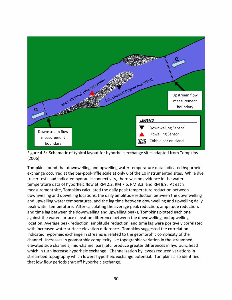
90

Figure 4.3: Schematic of typical layout for hyporheic exchange sites adapted from Tompkins (2006).

Tompkins found that downwelling and upwelling water temperature data indicated hyporheic exchange occurred at the bar-pool-riffle scale at only 6 of the 10 instrumented sites. While dye tracer tests had indicated hydraulic connectivity, there was no evidence in the water temperature data of hyporheic flow at RM 2.2, RM 7.6, RM 8.3, and RM 8.9. At each measurement site, Tompkins calculated the daily peak temperature reduction between downwelling and upwelling locations, the daily amplitude reduction between the downwelling and upwelling water temperatures, and the lag time between downwelling and upwelling daily peak water temperature. After calculating the average peak reduction, amplitude reduction, and time lag between the downwelling and upwelling peaks, Tompkins plotted each one against the water surface elevation difference between the downwelling and upwelling location. Average peak reduction, amplitude reduction, and time lag were positively correlated with increased water surface elevation difference. Tompkins suggested the correlation indicated hyporheic exchange in streams is related to the geomorphic complexity of the channel. Increases in geomorphic complexity like topographic variation in the streambed, elevated side channels, mid-channel bars, etc. produce greater differences in hydraulic head which in turn increase hyporheic exchange. Channelization by levees reduced variations in streambed topography which lowers hyporheic exchange potential. Tompkins also identified that low flow periods shut off hyporheic exchange.

Downstream flow

measurement

boundary

Upstream flow

measurement

boundary

Downwelling Sensor

Upwelling Sensor

Cobble bar or island

LEGEND

91

4.3 Data

I obtained directly from Tompkins the measured data from his Deer Creek study. Table 4.1 summarizes the period of available data for each instrumented site that had evidence of hyporheic exchange according to Tompkins. Water temperature was measured by Tompkins every 15 minutes or every hour using Maxim Integrated DS1922L iButton sensors with a resolution of 0.06oC and an accuracy of ± 0.5oC. Temperature sensors were calibrated before and after deployment under the range of conditions they experienced in the field to verify that they performed to specifications. Data were downloaded in the field every four weeks. Tompkins calibrated sensors pre- and post-deployment both by themselves and inside the PVC housings used during the instrumentation to verify the housings did not affect temperature measurements. Downwelling sensors were placed inside small PVC housings with fiberglass mesh that allowed unobstructed flow around the sensor. The PVC housings were then zip-tied to a piece of steel rebar anchored into the streambed at each downwelling site. Upwelling water temperature sensors were placed inside PVC piezometers with a 15 cm perforated section, then the piezometers were buried approximately 23 cm below the streambed at each upwelling site. As a result downwelling sensors measured the stream temperature at the streambed, while upwelling sensors sampled the water temperature 8 cm to 23 cm below the streambed.

Tompkins assessed the groundwater contributions at each study site by synoptic flow measurements upstream and downstream of the hyporheic exchange sites in early September. Tompkins adopted the standard operating guidelines for synoptic flow calculations detailed by Buchanan and Somers (1969). Positive differences in flow between the upstream and downstream site boundary would indicate the stream was gaining, while negative differences would indicate the stream was losing. Measurement error ranged from ± 5% to ± 10% so Tompkins estimated that there was no net change in flow at sites when there was less than a 10% difference between upstream and downstream flow. The change in flow across all hyporheic sites except RM 2.7 was calculated by Tompkins as less than 10% of the surface flow indicating there were no significant inflows of groundwater. While the surface flow decreased 17% across RM 2.7, stream temperature was not affected since the stream was losing and there was no net influx of groundwater.

The difference in the water surface elevations between the downwelling and upwelling locations was measured by Tompkins at each hyporheic site to determine the hydraulic head driving subsurface flow through the streambed. Water surface elevations were measured only once at each site on September 9 or September 10, 2005. The variability in water surface elevations with seasonal changes in flow is unknown, so caution must be exercised using the reported hydraulic head measurements when surface flow differs from conditions on September 9 and 10, 2005.

92

Table 4.1: Deer Creek data identified by Tompkins as having evidence of hyporheic flow

Site name

Period of record Frequency of temperature

measurement

Difference in water surface elevation between downwelling and upwelling

locations on September 9 – 10, 2005 (m)

RM 2.7 7/8/05 - 10/21/05 15-min 0.98

RM 5.0 7/3/05 - 12/15/05 Hourly 0.79

RM 5.7 7/10/05 - 10/21/05 15-min 2.07

RM 6.0 7/9/05 - 10/23/05 15-min 0.98

RM 6.9 7/9/05 - 10/22/05 Hourly 1.19

RM 9.9 7/31/05 - 10/22/05 15-min 1.49

I obtained from the USGS and California Department of Water Resources (DWR) surface flow data for Deer Creek and its diversions for 2005 with the details summarized in Table 4.2. USGS measured surface flow at 15-minute intervals at three locations in the Deer Creek watershed (Figure 4.4). USGS measured the surface water flows within Deer Creek 10.5 miles upstream of the Deer Creek-Sacramento River confluence (RM 10.5). DWR measured the flow removed from Deer Creek at the DCID diversion dam at RM 10 (DCID). DWR also measured surface flow in Deer Creek below the SVRIC main diversion dam at RM 4.1. Flow data are not available in 2005 for the Cone-Kimball diversion at RM 6.4 or the SVRIC main diversion dam at RM 4.1. At RM 5.0, RM 5.7, and RM 6.0, surface flow, Q, can be estimated using the available measured flow data and the estimated flows diverted by the Cone-Kimball and SVRIC main dams:

𝑄 = 𝑄𝑅𝑀 10.5 − 𝑄𝐷𝐶𝐼𝐷 − 𝛽𝐶𝐾𝑄𝑆𝑉𝑅𝐼𝐶 (4.1)

where QRM 10.5 is the measured flow in Deer Creek at river mile 10.5, QDCID is the measured flow diverted at DCID, βCK is the fraction of the flow diverted by SVRIC at the Cone-Kimball diversion, and QSVRIC is the total amount diverted by SVRIC. The fraction of the flow diverted by SVRIC at Cone-Kimball varied with time, but can be estimated from the daily average diversion amounts calculated by DWR from 1997 – 2000 data (McManus, 2004). The total amount diverted by SVRIC is assumed to be the difference between surface flow below the DCID diversion dam and the flow measured at RM 4.1.

Table 4.2: Sources of surface flow data

Gauge Abbreviation

Gauge Name Source Period of Record Selected Frequency of data collection

RM 10.5 11383500 Deer Creek NR Vina, CA

USGS 1/1/2005 - 12/31/2005 15-min

DCID DCID Deer Creek Diversion near Vina

DWR 1/1/2005 - 12/31/2005 15-min

RM 4.1 Deer Creek below Stanford Vina Dam

DWR 1/1/2005 - 12/31/2005 15-min

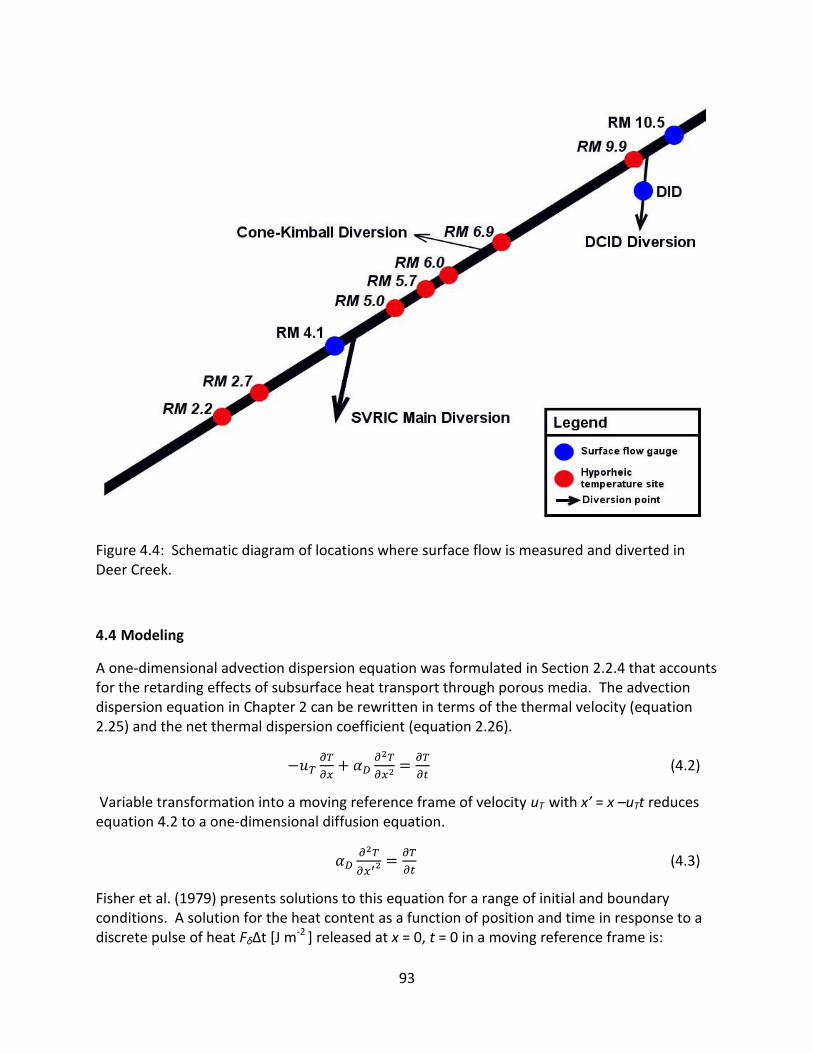
93

Figure 4.4: Schematic diagram of locations where surface flow is measured and diverted in Deer Creek.

4.4 Modeling

A one-dimensional advection dispersion equation was formulated in Section 2.2.4 that accounts for the retarding effects of subsurface heat transport through porous media. The advection dispersion equation in Chapter 2 can be rewritten in terms of the thermal velocity (equation 2.25) and the net thermal dispersion coefficient (equation 2.26).

−𝑢𝑇𝜕𝑇

𝜕𝑥+ 𝛼𝐷

𝜕2𝑇

𝜕𝑥2=

𝜕𝑇

𝜕𝑡 (4.2)

Variable transformation into a moving reference frame of velocity uT with x’ = x –uTt reduces equation 4.2 to a one-dimensional diffusion equation.

𝛼𝐷𝜕2𝑇

𝜕𝑥′2 =𝜕𝑇

𝜕𝑡 (4.3)

Fisher et al. (1979) presents solutions to this equation for a range of initial and boundary conditions. A solution for the heat content as a function of position and time in response to a discrete pulse of heat FδΔt [J m-2 ] released at x = 0, t = 0 in a moving reference frame is:

94

𝛿(𝑥′, 𝑡) =𝐹𝛿∆𝑡

√4𝜋𝛼𝐷𝑡exp [−

(𝑥′)2

4𝛼𝐷𝑡] (4.4)

When the heat input is a function of time, Fδ,in(t), the model for temperature distribution in space and time can be formulated by a Green’s function solution. Since the equation is linear in temperature and therefore heat content, individual heat pulses diffuse independently. When the solution is transformed back to a stationary reference frame, the heat content at x and t is the integral of the contributions from all prior heat pulses.

𝐻(𝑥, 𝑡) = ∫𝐹𝛿,𝑖𝑛(𝜏)

√4𝜋𝛼𝐷𝜏𝑒𝑥𝑝 (−

(𝑥−𝑢𝑇𝜏)2

4𝛼𝐷𝜏)

𝑡

−∞𝑑𝜏 (4.5)

For the Deer Creek sites the downwelling locations impose the incoming boundary condition at x = 0 as a time varying heat flux Fδ,in(t) which is dominated by advection. The downwelling heat flux is given by the time-varying advective heat flux given by:

𝐹𝛿,𝑖𝑛(𝑡) = 𝑢𝑇𝜌𝑚𝑐𝑚𝑇𝑤,𝑖𝑛(𝑡) (4.6)

where ρm is the density of the medium composed of pore filling water and the solid phase, and cm is the heat capacity of the water-saturated medium. The temperature at x and t can then be modeled as a summation of all the heat fluxes from 0 to t and divided by the density and heat capacity of the medium:

(4.7)

4.4.1 Model Checking

I checked the model represented by equation 4.7 by comparing modeled water temperature to water temperature calculated from an analytical solution. Fisher et al. (1979) provide the analytical solution to the advection dispersion equation in one dimension when there is a constant temperature boundary at x = 0 and the initial heat concentration is zero throughout the x domain.

𝐻(0, 𝑡) = 𝜌𝑤𝑐𝑤𝑇𝑜 0 < t < ∞ (4.8 (a))

𝐻(𝑥, 𝑡) = 0 x -> - ∞ (4.8 (b))

𝐻(𝑥, 0) = 0 -∞ < x < ∞ (4.9)

𝐻(𝑥 = 𝐿, 𝑡) = 𝜌𝑚𝑐𝑚𝑇𝑜

2[𝑒𝑟𝑓𝑐 (

𝐿−𝑢𝑇𝑡

√4𝛼𝐷𝑡) + 𝑒𝑟𝑓𝑐 (

𝐿+𝑢𝑇𝑡

√4𝛼𝐷𝑡) exp (

𝑢𝑇𝐿

𝛼𝐷)] (4.10)

Equation 4.10 can be normalized by noting that there are two nondimensional quantities in the expression. Rewriting equation 4.10 using the Peclet number (uT L/αD) and a nondimensional

𝑇(𝑥, 𝑡) = 𝐻(𝑥, 𝑡)

𝜌𝑚𝑐𝑚= ∑

𝑢𝑇𝑇𝑤,𝑖𝑛(𝑡 − 𝑗𝛥𝑡)∆𝑡

√4𝜋𝛼𝐷(𝑡 − 𝑗∆𝑡)𝑒𝑥𝑝 [−

(𝑥 − 𝑢𝑇(𝑡 − 𝑗∆𝑡))2

4𝛼𝐷(𝑡 − 𝑗∆𝑡)]

𝑡/∆𝑡

𝑗=0

95

time defined as time divided by the residence time if the system is purely advective, t* = t uT /L, produces:

𝑇(𝑃𝑒,𝑡∗)

𝑇𝑜=

1

2[𝑒𝑟𝑓𝑐 (

1−𝑡∗

√4 𝑡∗

𝑃𝑒

) + 𝑒𝑟𝑓𝑐 (1+𝑡∗

√4𝑡∗

𝑃𝑒

) 𝑒𝑃𝑒] (4.11)

The analytical solution and model were evaluated for Peclet numbers of 10, 30, and 100 to demonstrate the model’s applicability under the observed field conditions. Figure 4.5 plots the temperature calculated from the analytical solution and the model for these three different Peclet numbers with a nondimensional time step, Δt* = Δt uT /L, equal to 0.01. Agreement between the analytical and modeled water temperature at Pe > 10 indicates that equation 4.7 is being solved accurately under advection-dominated conditions. At the low Peclet number, the modeled water temperature is less than the analytical solution because the boundary and initial conditions are different between the analytical solution and the model. The analytical solution imposes a constant temperature boundary at x = 0 and is only valid for x > 0. The model imposes a time-varying heat source at x = 0 with a modeling domain of - ∞ < x < ∞ . As the Peclet number increases, the system becomes advection dominated and heat diffusion in the negative x direction decreases which improves the agreement between the two solutions. The nondimensional time step must be 0.01 or less to prevent numerical solution errors. Numerical errors become significant when the nondimensional time step is greater than 0.05.

96

Figure 4.5: Analytical and modeled temperature for (a) Pe = 10, (b) Pe = 30, (c) Pe = 100.

Equation 4.7 estimates the upwelling hyporheic water temperature under an advection-dominated system. The input parameters for the model and the derived retardation factor are listed in Table 4.3. Site specific input parameters include the time lag between the downwelling and upwelling temperature signal, tlag, the length of the hyporheic flow path, L,

0 0.5 1 1.5 2 2.5 3

x 105

0

2

4

6

8

10

Time, s

Te

mp

era

ture

, oC

Pe = 10

Analytical

Model

0 0.5 1 1.5 2 2.5 3

x 105

0

5

10

Time, s

Te

mp

era

ture

, oC

Pe = 30

Analytical

Model

0 0.5 1 1.5 2 2.5 3

x 105

0

5

10

Time, s

Te

mp

era

ture

, oC

Pe = 100

Analytical

Model

(c)

(b)

(a)

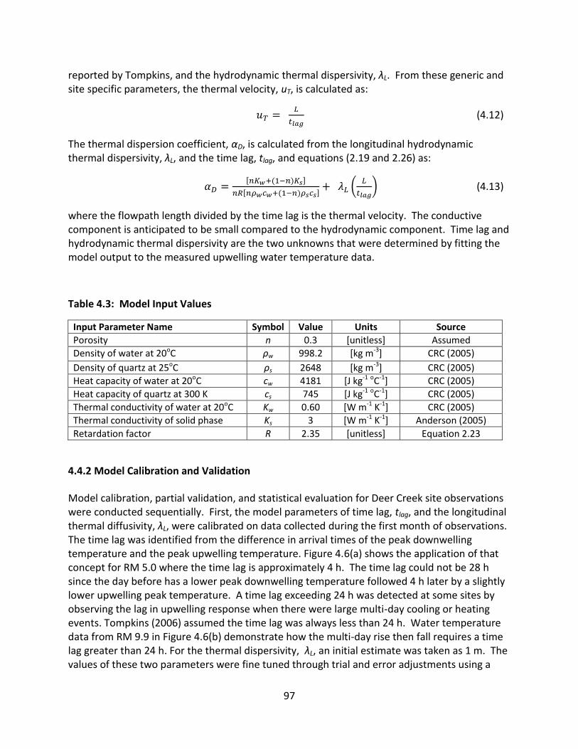
97

reported by Tompkins, and the hydrodynamic thermal dispersivity, λL. From these generic and site specific parameters, the thermal velocity, uT, is calculated as:

𝑢𝑇 = 𝐿

𝑡𝑙𝑎𝑔 (4.12)

The thermal dispersion coefficient, αD, is calculated from the longitudinal hydrodynamic thermal dispersivity, λL, and the time lag, tlag, and equations (2.19 and 2.26) as:

𝛼𝐷 =[𝑛𝐾𝑤+(1−𝑛)𝐾𝑠]

𝑛𝑅[𝑛𝜌𝑤𝑐𝑤+(1−𝑛)𝜌𝑠𝑐𝑠]+ 𝜆𝐿 (

𝐿

𝑡𝑙𝑎𝑔) (4.13)

where the flowpath length divided by the time lag is the thermal velocity. The conductive component is anticipated to be small compared to the hydrodynamic component. Time lag and hydrodynamic thermal dispersivity are the two unknowns that were determined by fitting the model output to the measured upwelling water temperature data.

Table 4.3: Model Input Values

Input Parameter Name Symbol Value Units Source

Porosity n 0.3 [unitless] Assumed

Density of water at 20oC ρw 998.2 [kg m-3] CRC (2005)

Density of quartz at 25oC ρs 2648 [kg m-3] CRC (2005)

Heat capacity of water at 20oC cw 4181 [J kg-1 oC-1] CRC (2005)

Heat capacity of quartz at 300 K cs 745 [J kg-1 oC-1] CRC (2005)

Thermal conductivity of water at 20oC Kw 0.60 [W m-1 K-1] CRC (2005)

Thermal conductivity of solid phase Ks 3 [W m-1 K-1] Anderson (2005)

Retardation factor R 2.35 [unitless] Equation 2.23

4.4.2 Model Calibration and Validation

Model calibration, partial validation, and statistical evaluation for Deer Creek site observations were conducted sequentially. First, the model parameters of time lag, tlag, and the longitudinal thermal diffusivity, λL, were calibrated on data collected during the first month of observations. The time lag was identified from the difference in arrival times of the peak downwelling temperature and the peak upwelling temperature. Figure 4.6(a) shows the application of that concept for RM 5.0 where the time lag is approximately 4 h. The time lag could not be 28 h since the day before has a lower peak downwelling temperature followed 4 h later by a slightly lower upwelling peak temperature. A time lag exceeding 24 h was detected at some sites by observing the lag in upwelling response when there were large multi-day cooling or heating events. Tompkins (2006) assumed the time lag was always less than 24 h. Water temperature data from RM 9.9 in Figure 4.6(b) demonstrate how the multi-day rise then fall requires a time lag greater than 24 h. For the thermal dispersivity, λL, an initial estimate was taken as 1 m. The values of these two parameters were fine tuned through trial and error adjustments using a

98

visual assessment of fit which was later quantified by the root mean square error (RMSE). RMSE was selected as the best means of quantifying the variation between measured and modeled upwelling temperature.

Figure 4.6: (a) The peak upwelling water temperature at RM 5.0 occurred approximately 4 h after the peak downwelling temperature. (b) Multi-day rises and falls in the downwelling and upwelling water temperature peaks at RM 9.9 show the time lag was greater than 24 h.

The second phase in modeling was to test if the model parameters determined for the first month of observations could represent subsequent months in a partial validation of the model. In the strict sense of model validation, one would like to take a calibrated model and apply it to a new site with different physical and meteorological conditions. That is not possible at this time with the state of the art in hyporheic flow analysis.

The time lag parameter was modified following the observation by Tompkins that the time lag increased at a particular site over the period of July through December. Given the decrease in average water temperature over the summer and fall period, the time lag was modified each month to account for the increased viscosity of water. The time lag is related to the Darcy velocity by:

07/12 07/13 07/14 07/15

22

24

26

28

30

32

34

36

2005 Date

Te

mp

era

ture

, oC

RM 5.0

Measured Downwelling

Measured Upwelling

08/27 08/28 08/29 08/30 08/31 09/01 09/02

19

20

21

22

23

24

25

2005 Date

Te

mp

era

ture

, oC

RM 9.9

Measured Downwelling

Measured Upwelling~31 h

~4 h (a)

(b)

99

𝑡𝑙𝑎𝑔 = 𝑛𝑅𝐿

𝑢𝑤 (4.14)

Darcy’s Law is utilized to distinguish the dependence of the velocity on fluid and aquifer properties through:

𝑢𝑤 = 𝑘𝑔

𝜈 ∆ℎ

𝐿 (4.15)

where k is the permeability of the media, g is gravitational acceleration, ν is kinematic viscosity of the water, and Δh is the head loss over the flow length L. Following substitution of the expression for Darcy velocity into the time lag expression, the time lag’s dependence on fluid and porous media properties are:

𝑡𝑙𝑎𝑔 = 𝑛𝑅𝐿2𝜈

𝑘𝑔 𝛥ℎ (4.16)

While the flow path, L, and the media permeability, k, are assumed constant, the head loss, Δh, is controlled by the channel bed morphology and water surface elevations. Under flow conditions where the head loss can be assumed constant, the time lag is proportional to the kinematic viscosity, and the time lag under average water temperature conditions, 𝑇1̅, is used to estimate the time lag under average water temperature conditions, 𝑇2̅, by:

𝑡𝑙𝑎𝑔(𝑇2̅) = 𝑡𝑙𝑎𝑔(𝑇1̅)𝜈(𝑇2̅̅ ̅)

𝑣(𝑇1̅̅ ̅) (4.17)

The time lag parameter was adjusted monthly using average monthly surface water temperatures at each downwelling site. Variations in the surface flow rate could alter the head loss across the flow path at a site and possibly compromise this scaling argument that assumes Δh is constant. The time lag parameter was recalibrated following a high flow event when observations justified it.

A number of different methods of presenting the data and model results are utilized given the site specific parameter fitting and individual site features. Time series comparison of measured downwelling and upwelling temperatures are plotted along with model predicted upwelling temperature, but such plots become difficult to read for periods exceeding 10 days. Results are therefore presented over 7 to 10 day periods showing modeled and measured upwelled temperatures. Additionally, an instantaneous error is calculated for each upwelled measurement by:

Error = 𝑇𝑈𝑝𝑤𝑒𝑙𝑙𝑖𝑛𝑔,𝑚𝑒𝑎𝑠𝑢𝑟𝑒𝑑 − 𝑇𝑈𝑝𝑤𝑒𝑙𝑙𝑖𝑛𝑔,𝑚𝑜𝑑𝑒𝑙𝑒𝑑 (4.18)

with the error plotted against the measured upwelling temperature and using different colored symbols to distinguish the months. The model as formulated conserves the heat present in the measured downwelling temperature, so positive errors indicate the measured upwelling temperature signal has more heat than the measured downwelling temperature signal. A simpler one to one comparison of measured versus modeled upwelling provides limited model evaluation since most of the time there is less than a few degrees difference between observed and modeled temperatures. Visual parameter fitting and instantaneous error plots were

100

supported by calculating the root mean square error (RMSE) over the calibration period, validation period, and a composite of both periods. The RMSE for a site excluded the initial model runup period which was taken as two days or twice the time lag for the initial month of data, whichever is longer.

These procedures were modified when there were sudden changes in flow rate at a site that caused the modeled temperature to deviate from the observations. In some cases the model required re-calibration of the time lag following the flow event and in other cases the model output was not representative of the observed upwelling temperature for any set of parameters. Under these transient and altered conditions, modeled temperatures were not included within the plots or used in statistical measures of model fit.

4.5 Results by River Mile (RM)

The upwelled water temperature model was evaluated at the six Deer Creek sites where Tompkins said there was hyporheic exchange. Results are presented in the order of increasing modeling complexity rather than by river mile. There was one site where the model was not applicable and this site is discussed first. The next grouping includes three sites where a single hyporheic flow path was reasonable. Finally, there are two sites where the data suggested a one-dimensional heat transport model was unable to describe the upwelling temperature data, but the model provided insight into physical processes occurring at these locations.

Table 4.4 provides a summary of the modeling efforts organized by river mile. RM 6.0 is included for completeness since Tompkins indicated there was hyporheic flow at this site, but that conclusion is not supported by this analysis. For the three sites that where the model provided a good representation of the observations, Table 4.4 details the calibration period for time lag, the other months where time lag was predicted, and if re-calibration of the time lag was necessary. Periods where the model did not represent the observed data are indicated with “n/a.” Numerical estimates of model errors are included in the last column of the table. In the calculation of the model errors, data were excluded from transition periods that lasted one day or the time lag, whichever was greater, along with obvious errors in the measurements, flagged by an absolute difference between the model and measurement greater than 3oC. At two of the monitoring sites, RM 2.7 and RM 6.9, the model did not fit the observations, but there was a benefit in having best fit model predictions compared with observations.

4.5.1 RM 6.0

Hyporheic flow did not occur between the downwelling and upwelling locations at RM 6.0 because the time lag between the measured downwelling and upwelling daily peak temperatures was unrealistic. The time offset at RM 6.0 was less than an hour even though the distance between the measurement locations was 30.9 m (Figure 4.7). This would require a Darcy velocity of 0.006 m s-1 to transport heat between the downwelling and upwelling location. Typical subsurface Darcy velocities are between 10-6 m s-1 and 10-5 m s-1 (Hatch et al.,

101

2010), while the Darcy velocity in hyporheic transport ranges from 10-7 m s-1 to 10-3 m s-1 (Burkholder et al., 2008). Darcy velocities greater than 10-4 m s-1 are rare and are only associated with recently reworked channel features (Burkholder et al., 2008). A calculation of the hydrualic conductivity at this site can arrive at the same conclusion that there was no hyporheic flow. The hydraulic conductivity is estimated from the water surface elevation difference (Table 4.1), the distance between the downwelling and upwelling locations, and an estimate of the Darcy velocity from the observed time lag (Equation 2.25). The calculated hydraulic conductivity (Equation 2.11) was on the order of 0.2 m s-1 which is unrealistically large. Typical hydraulic conductivities in streambeds are 10-4 m s-1 to 10-7 m s-1 (Hatch et al., 2010), but have been found to be as large as 0.07 m s-1 (Burkholder et al., 2008). The estimated value exceeds this range, and thus, hyporheic flow is highly unlikely at this site.

The observed time offset was likely caused by a delayed response at the upwelling sensor due to local, vertical heat transport from the overlying water. Tompkins placed the downwelling temperature sensors at the streambed surface while the upwelling temperature sensors were buried between 8 cm and 23 cm below the streambed. The sensor located at the upwelling location likely recorded a heat signal from the overlying water column delayed by advection and dispersed by conduction of heat within the local sediment bed.

Figure 4.7: A time offset of less than an hour between the measured downwelling and upwelling water temperatures indicate that hyporheic flow did not occur between these locations at RM 6.0.

07/20 07/21 07/22 07/23 07/24 07/25

22

24

26

28

30

32

2005 Date

Te

mp

era

ture

, oC

RM 6

Downwelling Temperature

Upwelling Temperature

102

Table 4.4: Summary of modeling effort at Deer Creek sites

Site (River Mile)

Flowpath length [m]

Date Interval Parameter Estimation Method

tlag [h]

λL

[m]

Composite RMSE [oC ]

2.7* 27.4

7/08 – 7/24 Fitted 6 2

n/a 7/24 – 9/09 n/a n/a n/a

9/09 – 9/30 Predicted 6.9 2

10/01 – 10/21 Predicted 7.6 2

15.2

7/5 - 7/31 Fitted 4.5 1.5

0.57

8/01 - 8/31 Predicted 4.7 1.5

9/01 - 9/30 Predicted 5.3 1.5

10/01 - 10/31 Predicted 5.8 1.5

11/01 - 11/07 Predicted 6.8 1.5

11/08 – 11/09 n/a n/a n/a

11/10 - 11/30 Fitted 11.3 1.5

12/01 - 12/04 n/a n/a n/a

12/05 - 12/15 Predicted 12.2 1.5

5.7 22

7/14 - 7/31 Fitted 45 0.5

0.38 8/01 - 8/31 Predicted 47 0.5

9/01 - 9/30 Predicted 52 0.5

10/01 - 10/21 Predicted 57 0.5

6.0† 30.9 7/10 - 10/23 n/a n/a n/a n/a

6.9* 24

7/11 - 7/29 Fitted 7.5 2

n/a

7/30 – 7/31 Fitted 12 2

8/01 – 8/31 Predicted 12.5 2

9/01 – 9/30 Predicted 14.0 2

10/01 – 10/22 Predicted 15.4 2

9.9 24.4

8/3 - 8/31 Fitted 34 1

0.29 9/01 - 9/30 Predicted 38 1

10/01 - 10/22 Predicted 42 1

* Model was not applicable but used to demonstrate other processes. †Site had no evidence of hyporheic flow.

5.0

10

2

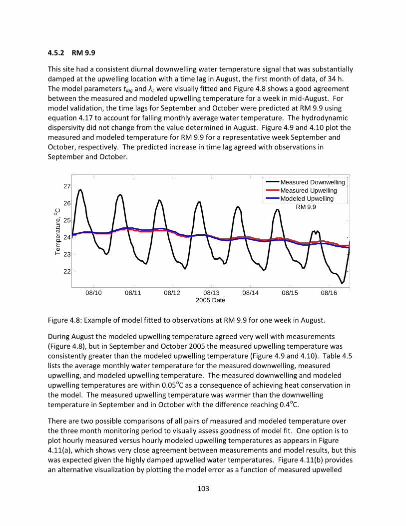
103

4.5.2 RM 9.9

This site had a consistent diurnal downwelling water temperature signal that was substantially damped at the upwelling location with a time lag in August, the first month of data, of 34 h. The model parameters tlag and λL were visually fitted and Figure 4.8 shows a good agreement between the measured and modeled upwelling temperature for a week in mid-August. For model validation, the time lags for September and October were predicted at RM 9.9 using equation 4.17 to account for falling monthly average water temperature. The hydrodynamic dispersivity did not change from the value determined in August. Figure 4.9 and 4.10 plot the measured and modeled temperature for RM 9.9 for a representative week September and October, respectively. The predicted increase in time lag agreed with observations in September and October.

Figure 4.8: Example of model fitted to observations at RM 9.9 for one week in August.

During August the modeled upwelling temperature agreed very well with measurements (Figure 4.8), but in September and October 2005 the measured upwelling temperature was consistently greater than the modeled upwelling temperature (Figure 4.9 and 4.10). Table 4.5 lists the average monthly water temperature for the measured downwelling, measured upwelling, and modeled upwelling temperature. The measured downwelling and modeled upwelling temperatures are within 0.05oC as a consequence of achieving heat conservation in the model. The measured upwelling temperature was warmer than the downwelling temperature in September and in October with the difference reaching 0.4oC.

There are two possible comparisons of all pairs of measured and modeled temperature over the three month monitoring period to visually assess goodness of model fit. One option is to plot hourly measured versus hourly modeled upwelling temperatures as appears in Figure 4.11(a), which shows very close agreement between measurements and model results, but this was expected given the highly damped upwelled water temperatures. Figure 4.11(b) provides an alternative visualization by plotting the model error as a function of measured upwelled

08/10 08/11 08/12 08/13 08/14 08/15 08/16

22

23

24

25

26

27

2005 Date

Te

mp

era

ture

, oC

RM 9.9

Measured Downwelling

Measured Upwelling

Modeled Upwelling

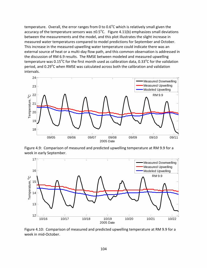
104

temperature. Overall, the error ranges from 0 to 0.6oC which is relatively small given the accuracy of the temperature sensors was ±0.5oC. Figure 4.11(b) emphasizes small deviations between the measurements and the model, and this plot illustrates the slight increase in measured water temperatures compared to model predictions for September and October. This increase in the measured upwelling water temperature could indicate there was an external source of heat or a multi-day flow path, and this common observation is addressed in the discussion of RM 6.9 results. The RMSE between modeled and measured upwelling temperature was 0.15oC for the first month used as calibration data, 0.33oC for the validation period, and 0.29oC when RMSE was calculated across both the calibration and validation intervals.

Figure 4.9: Comparison of measured and predicted upwelling temperature at RM 9.9 for a week in early September.

Figure 4.10: Comparison of measured and predicted upwelling temperature at RM 9.9 for a week in mid-October.

09/05 09/06 09/07 09/08 09/09 09/10 09/11

18

19

20

21

22

23

24

2005 Date

Te

mp

era

ture

, oC RM 9.9

Measured Downwelling

Measured Upwelling

Modeled Upwelling

10/16 10/17 10/18 10/19 10/20 10/21 10/2212

13

14

15

16

17

2005 Date

Te

mp

era

ture

, oC RM 9.9

Measured Downwelling

Measured Upwelling

Modeled Upwelling

105

Figure 4.11: Model comparison with observations at RM 9.9 (a) Measured and modeled upwelled temperature (b) Error between the measured and modeled upwelling temperature.

12 14 16 18 20 22 24 26 2812

14

16

18

20

22

24

26

28

Measured Upwelling Temperature, oC

Mo

de

led

Up

we

llin

g T

em

pe

ratu

re, o

C

RM 9.9

August

September

October

1:1 Line

14 15 16 17 18 19 20 21 22 23 24 25- 1.0

- 0.8

- 0.6

- 0.4

- 0.2

0.0

0.2

0.4

0.6

0.8

1.0

Err

or:

Me

asu

red

-Mo

de

led

Te

mp

era

ture

, oC

Measured Upwelling Temperature, oC

RM 9.9

August

September

October

(a)

(b)

106

Table 4.5: Monthly average water temperature for RM 9.9

Month Avg Measured Downwelling Temperature [oC]

Avg Measured Upwelling Temperature [oC]

Avg Modeled Upwelling Temperature [oC]

August 23.04 23.16 23.05

September 18.43 18.73 18.45

October 14.63 15.00 14.68

Surface flow in Deer Creek at RM 9.9 varied little during the monitoring period (Figure 4.12). There were no variations in the measured upwelling temperature that corresponded to changes in surface flow. The small fluctuations in flow rate in September and October did not cause any deviations between measured and modeled upwelled water temperature.

Figure 4.12: Surface flow at RM 9.9.

4.5.3 RM 5.7

Upwelling water temperature at RM 5.7 was successfully modeled through calibration and partial validation using the one-dimensional heat transport model driven by measured downwelling water temperature. The model parameters tlag and λL were calibrated during the first month of monitoring in July with Figure 4.13 showing a representative week. A time lag of 45 h was needed for the model to replicate the delayed response of the measured upwelling water temperature to the cooler day on 7/21. A hydrodynamic thermal dispersivity of 0.5 m was determined for July and was not changed during the entire monitoring period. The model was then partially validated in the months of August, September, and October by only correcting the time lag for viscosity effects based on average monthly temperatures. Figure 4.14 plots the measured downwelling and upwelling temperature data along with the modeled upwelling temperature for representative weeks in August, September, and October. As the

Jul Aug Sep Oct0.0

0.5

1.0

1.5

2.0

2.5

3.0

3.5

4.0

2005 Date

Flo

w, m

3s

-1

107

average water temperature cools, the time lag increases and the amplitude of daily fluctuations in upwelled water temperature decreases with greater opportunity for dispersion as observed in September and more so in October. The model was able to capture the daily and seasonal trends in upwelled water temperature with only two model parameters. Similar to the RM 9.9 site, the time lag and the hydrodynamic thermal dispersivity were visually calibrated from data collected in the first month. Given the damped upwelling signal, the model is relatively insensitive to variations in the dispersivity.

Figure 4.13: Measured and model calibrated upwelled water temperatures for a one-week period in July at RM 5.7.

07/18 07/19 07/20 07/21 07/22 07/23 07/24

22

24

26

28

30

32

34

2005 Date

Te

mp

era

ture

, oC

RM 5.7

Measured Downwelling

Measured Upwelling

Modeled Upwelling

108

Figure 4.14: Measured and model predicted water temperature at the RM 5.7 upwelling location for a week in (a) early August (b) early September (c) early October.

08/03 08/04 08/05 08/06 08/07 08/08 08/09

22

24

26

28

30

32

34

2005 Date

Te

mp

era

ture

, o C

RM 5.7

Measured Downwelling

Measured Upwelling

Modeled Upwelling

09/03 09/04 09/05 09/06 09/07 09/08 09/09

18

20

22

24

26

28

2005 Date

Te

mp

era

ture

, oC

RM 5.7

Measured Downwelling

Measured Upwelling

Modeled Upwelling

10/03 10/04 10/05 10/06 10/07 10/08 10/09

14

16

18

20

22

2005 Date

Te

mp

era

ture

, oC RM 5.7

Measured Downwelling

Measured Upwelling

Modeled Upwelling

(a)

(c)

(b)

109

The difference between the measured and the modeled upwelling temperatures are compared in Figure 4.15 with the plot covering the complete monitoring period from July to October. The modeled upwelled temperature in July is a generally unbiased estimate of the measured upwelled temperature with the exception of one large fluctuation in error from 7/22 to 7/24. For later months there is an obvious bias in the error with measured upwelled temperatures slightly greater than modeled upwelled temperatures. This bias increases from an average of about 0.2oC in August to about 0.4oC in September and October. These results are also quantified in Table 4.6 with the average monthly water temperatures measured at the downwelling and upwelling sites along with the average monthly modeled upwelling temperature. As with RM 9.9, there is conservation of heat between the measured downwelling temperature and the modeled upwelling temperature. The slight increase in measured monthly average water temperature at the upwelling location suggests there was an external heat source or a multi-day flow path which is addressed in the discussion of RM 6.9 results. The RMSE between modeled and measured upwelling temperature was 0.24oC during the calibration period, 0.40oC during the validation period, and 0.38oC for the entire monitoring period.

Figure 4.15: The error between the measured and the modeled temperature at RM 5.7 over the monitoring period.

Table 4.6: Monthly average water temperature for RM 5.7

Month Avg Measured Downwelling Temperature [oC]

Avg Measured Upwelling Temperature [oC]

Avg Modeled Upwelling Temperature [oC]

July 26.70 26.66 26.68

August 24.96 25.17 24.96

September 20.14 20.56 20.12

October 16.26 16.66 16.27

15 20 25 30-1

-0.5

0

0.5

1

Err

or:

Me

asu

red

-Mo

de

led

Te

mp

era

ture

, oC

Measured Upwelling Temperature, oC

RM 5.7

July

August

September

October

110

The daily average surface flow rate ranged from 1.7 m3s-1 to 3.0 m3s-1during the monitoring period (Figure 4.16). The September and October fluctuations in flow of about 10% did not alter the agreement between measured and modeled upwelling temperature.

Figure 4.16: Surface flow at RM 5.7.

4.5.4 RM 5.0

The model application at site RM 5.0 added some additional complexity to the discussion related to flow effects. The model calibration and validation were successful in reproducing time lags and daily peak temperatures from July through October, but in November and December high flow events required recalibration of the time lag. In July, model calibration led to a time lag of 4.5 h and a thermal dispersivity of 1.5 m. For the validation period of August through October, the predicted time lag increased using the correction for average monthly temperature according to equation 4.17 and the thermal dispersivity was not changed. For the calibration period and the validation period, the modeled upwelling temperature tracks the measured upwelling temperature, except there is no agreement between the model and the measurements during the low temperatures each day (Figure 4.17).

Jul Aug Sep Oct0

1

2

3

4

2005 Date

Flo

w, m

3s

-1

07/14 07/15 07/16 07/17 07/18 07/19 07/20

24

26

28

30

32

34

36

2005 Date

Te

mp

era

ture

, oC

RM 5.0

Measured Downwelling

Measured Upwelling

Modeled Upwelling(a)

111

Figure 4.17: The measured and modeled water temperatures at RM 5.0 (a) mid-July example of the calibration period, (b) mid-August example in validation period, (c) mid-September example in the validation period, and (d) mid-October example in validation period.

08/13 08/14 08/15 08/16 08/17 08/18 08/19

22

24

26

28

30

32

2005 Date

Te

mp

era

ture

, oC

RM 5.0

Measured Downwelling

Measured Upwelling

Modeled Upwelling

09/12 09/13 09/14 09/15 09/16 09/17 09/18 09/19

16

18

20

22

24

26

2005 Date

Te

mp

era

ture

, oC

RM 5.0

Measured Downwelling

Measured Upwelling

Modeled Upwelling

10/12 10/13 10/14 10/15 10/16 10/17 10/18 10/19

13

14

15

16

17

18

19

20

21

2005 Date

Te

mp

era

ture

, oC

RM 5.0

Measured Downwelling

Measured Upwelling

Modeled Upwelling

(d)

(c)

(b)

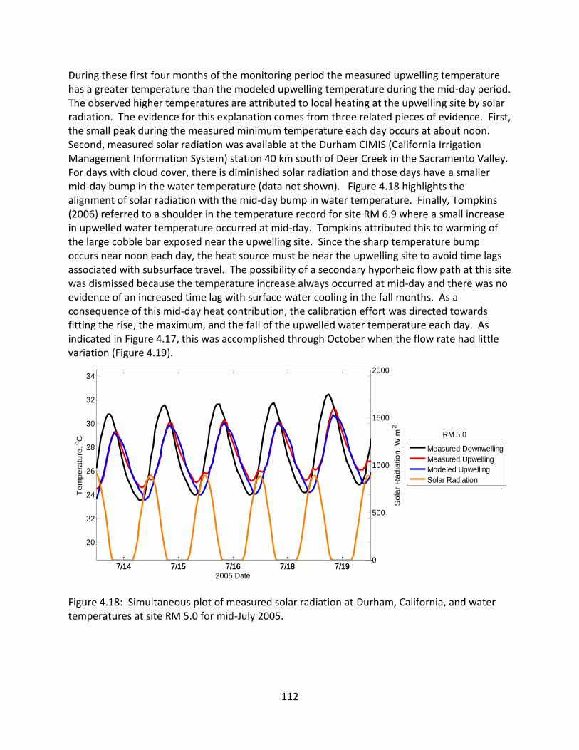
112

During these first four months of the monitoring period the measured upwelling temperature has a greater temperature than the modeled upwelling temperature during the mid-day period. The observed higher temperatures are attributed to local heating at the upwelling site by solar radiation. The evidence for this explanation comes from three related pieces of evidence. First, the small peak during the measured minimum temperature each day occurs at about noon. Second, measured solar radiation was available at the Durham CIMIS (California Irrigation Management Information System) station 40 km south of Deer Creek in the Sacramento Valley. For days with cloud cover, there is diminished solar radiation and those days have a smaller mid-day bump in the water temperature (data not shown). Figure 4.18 highlights the alignment of solar radiation with the mid-day bump in water temperature. Finally, Tompkins (2006) referred to a shoulder in the temperature record for site RM 6.9 where a small increase in upwelled water temperature occurred at mid-day. Tompkins attributed this to warming of the large cobble bar exposed near the upwelling site. Since the sharp temperature bump occurs near noon each day, the heat source must be near the upwelling site to avoid time lags associated with subsurface travel. The possibility of a secondary hyporheic flow path at this site was dismissed because the temperature increase always occurred at mid-day and there was no evidence of an increased time lag with surface water cooling in the fall months. As a consequence of this mid-day heat contribution, the calibration effort was directed towards fitting the rise, the maximum, and the fall of the upwelled water temperature each day. As indicated in Figure 4.17, this was accomplished through October when the flow rate had little variation (Figure 4.19).

Figure 4.18: Simultaneous plot of measured solar radiation at Durham, California, and water temperatures at site RM 5.0 for mid-July 2005.

7/14 7/15 7/16 7/18 7/19

20

22

24

26

28

30

32

34

2005 Date

Te

mp

era

ture

, oC

RM 5.0

7/14 7/15 7/16 7/18 7/190

500

1000

1500

2000

So

lar

Ra

dia

tio

n, W

m-2

Measured Downwelling

Measured Upwelling

Modeled Upwelling

Solar Radiation

113

Figure 4.19 Flow rate in Deer Creek at RM 5.0 for the period of July through October 2005.

The calibrated model could not be extended through November because of a high flow event on November 8 and 9 when the flow increased from less than 2 m3 s-1 to over 20 m3 s-1. Figure 4.20(a) shows the hydrograph for the month of November. Figure 4.20(b) includes the measured downwelling and upwelling temperatures through 11/9 along with the predicted upwelling temperatures from adjusting the July time lag parameter for the average water temperature in November giving tlag = 6.8 h. The predicted upwelled water temperature adequately represents the observed upwelled water temperature prior to the high flow period of 11/8 through 11/9. During the high flow period, the measured upwelled water temperature is very close to the downwelled water temperature indicating cessation of hyporheic flow. Increased surface flow likely lowered the hydraulic head driving hyporheic flow by reducing the difference in the water surface elevation between the downwelling and upwelling locations. Channel geomorphic cross sections and stage measurements during this time period were not available to test this hypothesis. The model predictions in Figure 4.20(b) diverged from the observed upwelling temperature when flow exceeded about 10 m3 s-1. After surface flow decreased on November 9, the predicted time lag of 6.8 h did not agree with the observations. Figure 4.20(c) includes model generated upwelling temperatures after recalibration with a fitted time lag of 11.3 h that adequately represented the remainder of the November observations. No adjustment was made in the thermal dispersivity.

Jul Aug Sep Oct Nov0

1

2

3

4

5

2005 Date

Flo

w, m

3s

-1

114

Figure 4.20: November measurements and model results at RM 5.0 (a) Flow hydrograph (b) Measured downwelling and upwelling water temperature with predicted upwelling water temperature based on time lag adjusted for the average November water temperature (tlag = 6.8 h) (c) Measured and modeled water temperature following recalibration with tlag = 11.3 h.

11/01 11/05 11/10 11/15 11/20 11/25 11/300

5

10

15

20

25

2005 Date

Flo

w, m

3s

-1

11/01 11/02 11/03 11/04 11/05 11/06 11/07 11/08 11/09

10

11

12

13

14

15

2005 Date

Te

mp

era

ture

, oC

RM 5.0

Measured Downwelling

Measured Upwelling

Modeled Upwelling

11/09 11/10 11/11 11/12 11/13 11/14 11/15 11/16 11/17 11/18

9

10

11

12

13

14

15

2005 Date

Te

mp

era

ture

, oC

RM 5.0

Measured Downwelling

Measured Upwelling

Modeled Upwelling

(a)

(b)

(c)

115

Data collection efforts at RM 5.0 extended into December and this allowed for continued testing of the temperature dependence of the time lags and the importance of high flow events. The December flow hydrograph in Figure 4.21(a) has a peak flow rate of over 50 m3 s-1 in the first few days of the month followed by a recession. Upwelling water temperature was modeled in December based on a time lag estimated by applying the temperature correction from equation 4.17 to the time lag recalibrated in the post high-flow event period for November. The hydrodynamic thermal dispersivity was maintained at a constant value. High flows above about 20 m3s-1 shut off hyporheic flow on 12/01 and hyporheic flow returned on 12/03 when the flow dropped below 10 m3s-1 as indicated in Figure 4.21(b) when the measured downwelling and upwelling temperatures were equal. Following resumption of hyporheic flow, the measured upwelling temperature signal had frequent shifts in its amplitude and phase until 12/09 when the measured upwelling temperature signal stabilized. Measured and predicted upwelled temperature agreed from 12/09 to the end of monitoring on 12/15. There is little to no evidence of small peaks in the upwelling temperature measurements that indicate solar heating of the water, which is probably reasonable in December.

There was not a consistent bias between the measured and modeled upwelling temperature during the measurement period at RM 5.0 (Figure 4.22). Table 4.7 presents average monthly water temperature for the downwelling, measured upwelling, and modeled upwelling temperature. Measured downwelling and modeled upwelling temperature were similar for all the six months of data as expected, but the measured upwelling temperature ranged from 0.25oC cooler to 0.25oC warmer. The individual error plot for all data in Figure 4.22 has far more scatter than in the sites discussed previously (RM 9.9 and RM 5.7). The main cause of this increased individual error is that the model did not represent the elevated upwelled water temperature during the mid-day period attributed to a local solar radiation heating. The magnitude of the error in the upwelled temperature is greater in July and August compared to November and December reflecting the seasonal dependence on solar radiation intensity. The majority of the daily error occurred when the peak attributed to solar radiation caused a mismatch between the measured and modeled upwelling temperature and significantly increased the RMSE. The RMSE between modeled and measured upwelling temperature was 0.64oC during the July calibration period, 0.56oC during the validation period from August to December, and 0.57oC for the entire monitoring period from July through December excluding the high flow event periods in November and December.

116

Figure 4.21: December observations and model results at RM 5.0 (a) Stream hydrograph (b) Measured water temperatures and predicted upwelling temperature with tlag = 12.2 h based on temperature correction of the late November recalibrated time lag of 11.3 h.

Table 4.7: Monthly average water temperature for RM 5.0 excluding high flow events in November and December

Month Avg Measured Downwelling Temperature [oC]

Avg Measured Upwelling Temperature [oC]

Avg Modeled Upwelling Temperature [oC]

July 26.60 26.35 26.58

August 25.07 25.18 25.08

September 20.17 20.43 20.18

October 15.52 15.40 15.54

November 10.59 10.62 10.65

December 6.42 6.51 6.43

12/01 12/03 12/05 12/07 12/09 12/11 12/13 12/150

10

20

30

40

50

2005 Date

Flo

w, m

3s

-1

12/01 12/03 12/05 12/07 12/09 12/11 12/13 12/153

4

5

6

7

8

9

10

11

2005 Date

Te

mp

era

ture

, oC RM 5.0

Measured Downwelling

Measured Upwelling

Modeled Upwelling

(a)

(b)

117

Figure 4.22: RM 5.0 error by month excluding data during the high flow events in November and December. Note that November includes the recalibrated time lag after 11/08.

4.5.5 RM 2.7

The data collected by Tompkins at RM 2.7 on Deer Creek within this semi-natural stream channel illustrate environmental effects that are not represented in the one-dimensional heat transfer model. As with the data collected at RM 5.0 there are solar radiation pulses reflected in the upwelling measurements with variable contributions to the upwelling signal. The RM 2.7 stream flow record also had sudden changes caused by water diversion practices that caused hyporheic flows to shutoff at sufficiently low flows. There is also evidence in the measured data of a heat imbalance between downwelling and upwelling temperatures that is explored at site RM 6.9 where the hyporheic flows were continuous in the monitoring period. While the one-dimensional heat transfer model for hyporheic flow is not capable of representing the observations, the model was useful in identifying what can be attributed to hyporheic flow and what phenomena are in addition to that mechanism.

Figure 4.23 contains the flow rate and the water temperature signals for the initial 10-day period of the monitoring program. The flow rate varies between 0.2 m3 s−1 and 0.34 m3 s−1 and has evidence of diurnal fluctuations caused by transpiration of riparian vegetation combined with sudden, sustained decreases in flow by upstream flow diversion for irrigation (Figure 4.23(a)). The downwelling water temperature measurements in Figure 4.23(b) have a well-defined periodicity each day of heating and cooling with a longer-term trend of general warming. The upwelled water temperature measurements show consistent evidence of two small peaks each day with one of the daily peaks occurring consistently around noon and is attributed to solar radiation heating. The second peak appears with a time lag of 6 h after the downwelling peak temperature for each day. Usually the noon-time solar radiation peak is lower in magnitude than the second, hyporheic flow peak, except during 7/18 and 7/19 when

5 10 15 20 25 30

-3

-2

-1

0

1

2

3E

rro

r: M

ea

su

red

-Mo

de

led

Te

mp

era

ture

, oC

Measured Upwelling Temperature, oC

RM 5.0

July

August

September

October

November: 1 to 8

November: 9 to 30

December

118

the solar radiation peak is greater. The hyporheic heat transport model was partially fitted to the measurements during this period with a time lag of 6 h and a thermal diffusivity of 2 m. Even though this thermal diffusivity is greater than used at any other site, the model cannot match the measured upwelling amplitude. Additionally, since heat is conserved between the downwelling measurements and the upwelling model output, there is clear evidence that the upwelling measurements are cooler than the downwelling data during this period. Again, data from RM 6.9 will provide a more complete record to explore a possible explanation based on a multi-day hyporheic flow path for that site.

Figure 4.23: Deer Creek RM 2.7 for the period noon on 7/08 to noon on 7/19 (a) Flow and (b) Measured and modeled water temperatures.

07/09 07/10 07/11 07/12 07/13 07/14 07/15 07/16 07/17 07/18 07/190

0.05

0.10

0.15

0.20

0.25

0.30

0.35

0.40

2005 Date

Flo

w, m

3s

-1

07/09 07/10 07/11 07/12 07/13 07/14 07/15 07/16 07/17 07/18 07/19

25

30

35

40

2005 Date

Te

mp

era

ture

, oC

RM 2.7

Measured Downwelling

Measured Upwelling

Modeled Upwelling

(a)

(b)

119

The effect of sudden changes in surface water flow rate is demonstrated in Figure 4.24. Late in the day of 7/23 the flow rate in Deer Creek dropped instantaneously from 0.20 m3 s−1 to 0.10 m3 s−1. That drop resulted in the downwelling and upwelling water temperature measurements becoming nearly equal starting late on 7/23 and this result was maintained through 9/8. The measured upwelling minimum temperatures do not correspond to the measured downwelling temperatures, and there is no evidence of a solar radiation bump after 7/24.

Figure 4.24: Deer Creek RM 2.7 for the period noon on 7/18 to noon on 7/29 (a) Flow and (b) Measured and modeled water temperatures with hyporheic flow ceasing on 7/24.

07/19 07/20 07/21 07/22 07/23 07/24 07/25 07/26 07/27 07/28 07/290

0.05

0.10

0.15

0.20

0.25

0.30

0.35

0.40

2005 Date

Flo

w, m

3s

-1

07/19 07/20 07/21 07/22 07/23 07/24 07/25 07/26 07/27 07/28 07/29

22

24

26

28

30

32

34

36

38

40

2005 Date

Te

mp

era

ture

, oC

RM 2.7

Measured Downwelling

Measured Upwelling

Modeled Upwelling

(a)

(b)

120

The low flow period was maintained through August and on 9/8 flow quickly rose above 0.10 m3 s−1 (Figure 4.25(a)). With the increase in flow the upwelled water temperature measurements showed an immediate transition from no evidence of solar radiation or hyporheic flow to multiple peaks each day (Figure 4.25(b)). The time lag parameter in the hyporheic temperature model was adjusted for the decreased average September water temperature, and there was reasonable agreement between observed and modeled time lag for the upwelling temperature signal. However, the model was not able to match upwelling temperature amplitude or spread.

Figure 4.25: Deer Creek RM 2.7 for the period noon on 9/04 to noon on 9/14 (a) Flow and (b) Measured and modeled water temperatures with hyporheic flow resuming on 9/09.

09/05 09/06 09/07 09/08 09/09 09/10 09/11 09/12 09/13 09/140

0.1

0.2

0.3

0.4

0.5

0.6

0.7

0.8

2005 Date

Flo

w, m

3s

-1

09/05 09/06 09/07 09/08 09/09 09/10 09/11 09/12 09/13 09/1418

20

22

24

26

28

30

2005 Date

Te

mp

era

ture

, oC

RM 2.7

Measured Downwelling

Measured Upwelling

Modeled Upwelling

(b)

(a)

121

In mid-September there was a sudden and short-duration drop in flow rate that provided additional support for the dependence of hyporheic flows on stream flows. In Figure 4.26, there are two dips in flow rate with the first dip on 9/17 from 0.4 m3 s−1 to 0.2 m3 s−1 causing no alteration of the upwelled water temperature signal. However, on 9/20 the flow dropped from 0.4 m3 s−1 to about 0.1 m3 s−1 for 12 h, and during this period there was an overlap between measured downwelling and upwelling temperatures. The model poorly represents the upwelling temperature during this mid-September period, but the model is useful in indicating when the hyporheic temperature peak is expected to arrive each day. During this period there are rapid changes in the dominance of the solar radiation and hyporheic flow temperature peaks each day with no obvious explanation.

Figure 4.26: Deer Creek RM 2.7 for the period noon on 9/13 to noon on 9/24 (a) Flow and (b) Measured and modeled water temperatures.

09/14 09/15 09/16 09/17 09/18 09/19 09/20 09/21 09/22 09/23 09/240

0.1

0.2

0.3

0.4

0.5

0.6

0.7

0.8

2005 Date

Flo

w, m

3s

-1

09/14 09/15 09/16 09/17 09/18 09/19 09/20 09/21 09/22 09/23 09/2416

18

20

22

24

26

28

2005 Date

Te

mp

era

ture

, oC

RM 2.7

Measured Downwelling

Measured Upwelling

Modeled Upwelling

(a)

(b)

122

Due to the truncated record during the long period where there was no hyporheic flow, there is a limited ability to assess overall heat balances. Table 4.8 presents the average monthly water temperature for the downwelling, measured upwelling, and modeled upwelling temperature including only the periods when there was hyporheic flow. Measured downwelling and modeled upwelling temperature were similar for all the months of data confirming the model conserved heat. Unlike other sites, there was a net loss in heat between downwelling and upwelling measurements in September while there was a net gain in heat between downwelling and upwelling in October. A visual inspection of the final ten days of record in October clearly shows the upwelled water was warmer than the downwelled stream water (Figure 4.27). The complete hyporheic flow record for site RM 6.9, discussed next, provides sufficient data to suggest that multiple-day flow paths may be responsible for the local heat imbalance.

Figure 4.27: Deer Creek RM 2.7 for the period noon on 10/3 to noon on 10/14 (a) Flow and (b) Measured and predicted water temperatures.

10/04 10/05 10/06 10/07 10/08 10/09 10/10 10/11 10/12 10/13 10/140

0.2

0.4

0.6

0.8

1.0

1.2

2005 Date

Flo

w, m

3s

-1

10/04 10/05 10/06 10/07 10/08 10/09 10/10 10/11 10/12 10/13 10/14

14

15

16

17

18

19

20

21

22

2005 Date

Te

mp

era

ture

, oC

RM 2.7

Measured Downwelling

Measured Upwelling

Modeled Upwelling

(a)

(b)

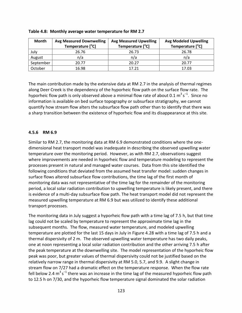
123

Table 4.8: Monthly average water temperature for RM 2.7

Month Avg Measured Downwelling Temperature [oC]

Avg Measured Upwelling Temperature [oC]

Avg Modeled Upwelling Temperature [oC]

July 26.76 26.73 26.78

August n/a n/a n/a

September 20.77 20.27 20.77

October 16.98 17.21 17.03

The main contribution made by the extensive data at RM 2.7 in the analysis of thermal regimes along Deer Creek is the dependency of the hyporheic flow path on the surface flow rate. The hyporheic flow path is only observed above a minimal flow rate of about 0.1 m3 s−1. Since no information is available on bed surface topography or subsurface stratigraphy, we cannot quantify how stream flow alters the subsurface flow path other than to identify that there was a sharp transition between the existence of hyporheic flow and its disappearance at this site.

4.5.6 RM 6.9

Similar to RM 2.7, the monitoring data at RM 6.9 demonstrated conditions where the one-dimensional heat transport model was inadequate in describing the observed upwelling water temperature over the monitoring period. However, as with RM 2.7, observations suggest where improvements are needed in hyporheic flow and temperature modeling to represent the processes present in natural and managed water courses. Data from this site identified the following conditions that deviated from the assumed heat transfer model: sudden changes in surface flows altered subsurface flow contributions, the time lag of the first month of monitoring data was not representative of the time lag for the remainder of the monitoring period, a local solar radiation contribution to upwelling temperature is likely present, and there is evidence of a multi-day subsurface flow path. The heat transport model did not represent the measured upwelling temperature at RM 6.9 but was utilized to identify these additional transport processes.

The monitoring data in July suggest a hyporheic flow path with a time lag of 7.5 h, but that time lag could not be scaled by temperature to represent the approximate time lag in the subsequent months. The flow, measured water temperature, and modeled upwelling temperature are plotted for the last 15 days in July in Figure 4.28 with a time lag of 7.5 h and a thermal dispersivity of 2 m. The observed upwelling water temperature has two daily peaks, one at noon representing a local solar radiation contribution and the other arriving 7.5 h after the peak temperature at the downwelling site. The model representation of the hyporheic flow peak was poor, but greater values of thermal dispersivity could not be justified based on the relatively narrow range in thermal dispersivity at RM 5.0, 5.7, and 9.9. A slight change in stream flow on 7/27 had a dramatic effect on the temperature response. When the flow rate fell below 2.4 m3 s−1 there was an increase in the time lag of the measured hyporheic flow path to 12.5 h on 7/30, and the hyporheic flow temperature signal dominated the solar radiation

124

contribution. Besides changes in surface flow, there was no identifiable cause for the increase in time lag.

Figure 4.28: Deer Creek RM 6.9 for the period 7/16 to 8/01 (a) Flow and (b) Water temperatures.

07/16 07/18 07/20 07/22 07/24 07/26 07/28 07/30 08/01

2.2

2.4

2.6

2.8

3

2005 Date

Flo

w, m

3s

-1

07/16 07/18 07/20 07/22 07/24 07/26 07/28 07/30 08/01

20

22

24

26

28

30

32

34

36

2005 Date

Te

mp

era

ture

, oC

RM 6.9

Measured Downwelling

Measured Upwelling

Modeled Upwelling

(a)

(b)

125

Figure 4.29: Deer Creek RM 6.9 for the period 8/01 to 8/15 (a) Flow and (b) Water temperatures.

For the August monitoring period, the hyporheic heat transfer model is compared with the observations using a re-calibrated time lag of 12.5 h while maintaining a thermal dispersivity of 2 m. The model is generally in good agreement with observations for the first half of August as indicated in Figure 4.28. The flow rate during this period is nearly constant with only a small decrease from approximately 2.3 m3 s-1 to about 2.1 m3 s−1, and the modeled upwelled water temperature closely matches the timing and the dispersion of the observations. The solar radiation contribution continues to be present at noon each day, but only makes a small contribution to the overall response. In contrast, the observed temperature signals in the second half of August are not well represented by the model. Figure 4.30 shows again a period of minimal changes in flow rate in this managed irrigation system. The upwelled temperature record shows considerable damping compared to the model that adequately represented the shape of the upwelling signal in the prior two-week interval. In addition, the solar radiation peak during this second half of August is no longer aligned with noon each day, and the solar

08/01 08/03 08/05 08/07 08/09 08/11 08/13 08/15

2

2.1

2.2

2.3

2.4

2.5

2005 Date

Flo

w, m

3s

-1

08/01 08/03 08/05 08/07 08/09 08/11 08/13 08/15

20

25

30

35

2005 Date

Te

mp

era

ture

, oC

RM 6.9

Measured Downwelling

Measured Upwelling

Modeled Upwelling

(a)

(b)

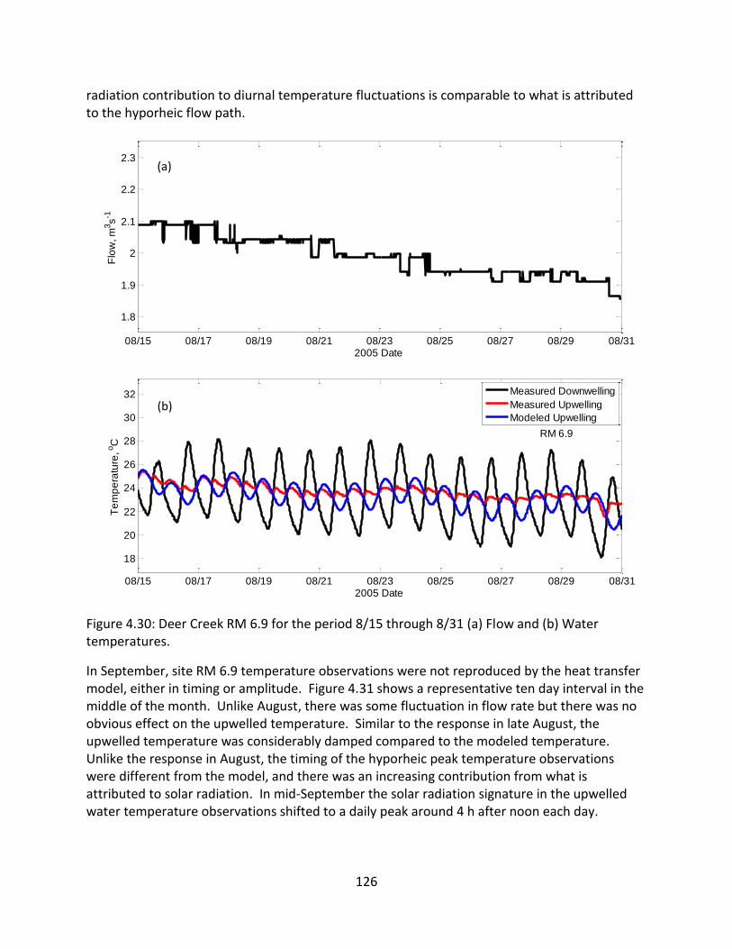
126

radiation contribution to diurnal temperature fluctuations is comparable to what is attributed to the hyporheic flow path.

Figure 4.30: Deer Creek RM 6.9 for the period 8/15 through 8/31 (a) Flow and (b) Water temperatures.

In September, site RM 6.9 temperature observations were not reproduced by the heat transfer model, either in timing or amplitude. Figure 4.31 shows a representative ten day interval in the middle of the month. Unlike August, there was some fluctuation in flow rate but there was no obvious effect on the upwelled temperature. Similar to the response in late August, the upwelled temperature was considerably damped compared to the modeled temperature. Unlike the response in August, the timing of the hyporheic peak temperature observations were different from the model, and there was an increasing contribution from what is attributed to solar radiation. In mid-September the solar radiation signature in the upwelled water temperature observations shifted to a daily peak around 4 h after noon each day.

08/15 08/17 08/19 08/21 08/23 08/25 08/27 08/29 08/31

1.8

1.9

2

2.1

2.2

2.3

2005 Date

Flo

w, m

3s

-1

08/15 08/17 08/19 08/21 08/23 08/25 08/27 08/29 08/31

18

20

22

24

26

28

30

32

2005 Date

Te

mp

era

ture

, oC

RM 6.9

Measured Downwelling

Measured Upwelling

Modeled Upwelling

(a)

(b)

127

Figure 4.31: Deer Creek RM 6.9 for the period 9/10 to 9/20 (a) Flow and (b) Water temperatures.

As Deer Creek seasonally cooled and the flow rate increased, the October record at RM 6.9 returned to a response closer to the model prediction. The model time lag for October was obtained by scaling the August time lag by the temperature shift from August to October without changing the thermal dispersivity. Two increases in flow rate during the October monitoring period caused responses in the upwelled water temperature. The first 11 days of October are reported in Figure 4.32 with a peak flow of 2.4 m3 s−1 on 10/4 and returning to base flow in a couple days. This minor increase in flow caused a sudden drop in the measured upwelled water temperature, but there was no improvement in the agreement between modeled and measured upwelled water temperature. The drop in upwelled water temperature persisted for the remainder of the record.

09/10 09/11 09/12 09/13 09/14 09/15 09/16 09/17 09/18 09/19 09/20

1.8

1.9

2

2.1

2.2

2.3

2.4

2005 Date

Flo

w, m

3s

-1

09/10 09/11 09/12 09/13 09/14 09/15 09/16 09/17 09/18 09/19 09/20

16

18

20

22

24

26

2005 Date

Te

mp

era

ture

, oC

RM 6.9

Measured Downwelling

Measured Upwelling

Modeled Upwelling

(a)

(b)

128

Figure 4.32: Deer Creek RM 6.9 from 10/01 to 10/11 (a) Flow and (b) Water temperatures.

The final ten day record from 10/12 to 10/22 is shown in Figure 4.33 for flow and temperature. There was an increase in flow from a base flow of about 2 m3 s−1 to a peak flow of 2.4 m3 s−1 on 10/16 and returning to the base flow on 10/17. This minor perturbation in flow caused a shift in response in the upwelled water temperature from one with no diurnal fluctuations prior to the flow event to a temperature response comparable in timing and magnitude to what the model predicted. Interestingly, there was no solar radiation signal present in the October upwelling monitoring data before, during, or after the flow event. Since 10/22 was the end of the monitoring period, there is no indication as to the persistence of the stream’s response to this flow perturbation or if the slight increase in flow rate on 10/21 caused the perturbation to persist.

10/01 10/02 10/03 10/04 10/05 10/06 10/07 10/08 10/09 10/10 10/11

1.8

1.9

2

2.1

2.2

2.3

2.4

2005 Date

Flo

w, m

3s

-1

10/01 10/02 10/03 10/04 10/05 10/06 10/07 10/08 10/09 10/10 10/11

12

14

16

18

20

22

24

2005 Date

Te

mp

era

ture

, oC

RM 6.9

Measured Downwelling

Measured Upwelling

Modeled Upwelling

(a)

(b)

129

Figure 4.33: Deer Creek RM 6.9 from 10/12 to 10/22(a) Flow and (b) Water temperatures.

Multiple flow pulses in the RM 6.9 record produced transient responses in upwelled stream temperature. The flow rate increases represent only a 10 to 20% increase above a base flow but cause a reproducible transient response in the observed upwelled temperature. The timing of the hyporheic peak in the measured upwelling temperature signal shifted on 7/29 when the surface flow decreased from 2.4 m3 s−1 to 2.2 m3 s-1 (Figure 4.28). Figure 4.34 captured the thermal response at the upwelling site for two flow events between 9/10 and 9/13 that resulted in a decrease in water temperature and a temporary increase in the amplitudes of the upwelling water temperature signal. In Figure 4.35 for the late September to early October period, there are two flow events, but the peak flow of the first event on 9/27 with a peak flow of 2.1 m3 s−1 did not cause a transient response in the upwelled temperature while the second peak of almost 2.4 m3 s−1 did cause a sharp drop in upwelled water temperature with no increase in diurnal temperature fluctuations. These examples illustrate that even small variations in surface flows alter the temperature response in Deer Creek at RM 6.9.

10/12 10/13 10/14 10/15 10/16 10/17 10/18 10/19 10/20 10/21 10/22

2

2.1

2.2

2.3

2.4

2.5

2005 Date

Flo

w, m

3s

-1

10/12 10/13 10/14 10/15 10/16 10/17 10/18 10/19 10/20 10/21 10/22

12

14

16

18

20

22

2005 Date

Te

mp

era

ture

, oC

RM 6.9

Measured Downwelling

Measured Upwelling

Modeled Upwelling

(a)

(b)

130

Figure 4.34: Deer Creek RM 6.9 from noon on 9/07 to noon on 9/16 (a) Flow and (b) Measured and modeled water temperatures.

09/08 09/09 09/10 09/11 09/12 09/13 09/14 09/15 09/161.6

1.8

2

2.2

2.4

2.6

2005 Date

Flo

w, m

3s

-1

09/08 09/09 09/10 09/11 09/12 09/13 09/14 09/15 09/16

16

18

20

22

24

26

28

2005 Date

Te

mp

era

ture

, oC

RM 6.9

Measured Downwelling

Measured Upwelling

Modeled Upwelling

(a)

(b)

131

Figure 4.35: Deer Creek RM 6.9 from noon on 9/26 to noon on 10/06 (a) Flow and (b) Measured and modeled water temperatures.

The short-term plots of downwelled and upwelled temperatures suggest there is a heat imbalance between downwelling and upwelling measurements. Table 4.9 provides monthly averages of water temperatures for RM 6.9 at Deer Creek. July had upwelling temperatures cooler, on average, than downwelling temperatures. August, September and October had just the opposite with the average monthly upwelling temperature warmer than the downwelling temperature. This observation is interpreted as a subsurface flow component that has a residence time of multiple days as the upwelled water temperature lags the stream water temperature. In support of this interpretation, the model output with a time lag of 3 days was compared with the observed downwelling and upwelling signals. To reduce the influence of diurnal fluctuations and multi-day warming and cooling events, the model output and the observations were averaged over 7-day intervals. Figure 4.36 is a plot of the 7-day average water temperatures that shows some agreement between the modeled upwelling temperature

09/26 09/27 09/28 09/29 09/30 10/01 10/02 10/03 10/04 10/05 10/061.6

1.8

2

2.2

2.4

2.6

2005 Date

Flo

w, m

3s

-1

09/26 09/27 09/28 09/29 09/30 10/01 10/02 10/03 10/04 10/05 10/06

12

14

16

18

20

22

24

2005 Date

Te

mp

era

ture

, oC

RM 6.9

Measured Downwelling

Measured Upwelling

Modeled Upwelling

(a)

(b)

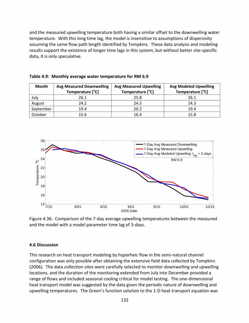
132

and the measured upwelling temperature both having a similar offset to the downwelling water temperature. With this long time lag, the model is insensitive to assumptions of dispersivity assuming the same flow path length identified by Tompkins. These data analysis and modeling results support the existence of longer time lags in this system, but without better site-specific data, it is only speculative.

Table 4.9: Monthly average water temperature for RM 6.9

Month Avg Measured Downwelling Temperature [oC]

Avg Measured Upwelling Temperature [oC]

Avg Modeled Upwelling Temperature [oC]

July 26.1 25.8 26.1

August 24.2 24.5 24.3

September 19.4 20.2 19.4

October 15.6 16.4 15.8

Figure 4.36: Comparison of the 7-day average upwelling temperatures between the measured and the model with a model parameter time lag of 3-days.

4.6 Discussion

This research on heat transport modeling by hyporheic flow in the semi-natural channel configuration was only possible after obtaining the extensive field data collected by Tompkins (2006). The data collection sites were carefully selected to monitor downwelling and upwelling locations, and the duration of the monitoring extended from July into December provided a range of flows and included seasonal cooling critical for model testing. The one-dimensional heat transport model was suggested by the data given the periodic nature of downwelling and upwelling temperatures. The Green’s function solution to the 1-D heat transport equation was

7/15 8/01 8/15 9/01 9/15 10/01 10/1514

16

18

20

22

24

26

28

2005 Date

Te

mp

era

ture

, oC RM 6.9

7-Day Avg Measured Downwelling

7-Day Avg Measured Upwelling

7-Day Avg Modeled Upwelling: tlag

= 3 days

133

straightforward and efficient compared to the extensive data processing of the measured temperature data required by the methods of Hatch et al. (2006) or Keery et al. (2007) and utilized by others (Vogt et al., 2010; Swanson and Cardenas, 2011; Gordon et al., 2012; Briggs et al., 2012).

The modeling approach had the additional advantage that there were only two calibration parameters for each site, a time lag and a thermal dispersivity. Three sites along Deer Creek demonstrated that the heat transport model could be calibrated using the initial month of monitoring data. Model parameters were extrapolated for the remainder of the monitoring period as a partial model validation. Additional monitoring sites along Deer Creek demonstrated conditions where hyporheic flow was not transporting heat, where solar radiation was compromising the upwelled water temperature record, and where fluctuations in flow rate were altering hyporheic flow. While the model was not adequate in describing observations at all sites, having a model to compare with observations was essential in identifying additional heat transport processes and possible anomalies in the monitoring data within this partially managed system.

The heat transport model parameters were successfully calibrated at three of the paired monitoring locations along Deer Creek (RM 9.9, RM 5.7, and RM 5.0). The time lag parameter was largely determined from a visual inspection of the downwelled and upwelled monitoring data and the thermal dispersivity had a limited range. The model was extended to the remaining monitoring data at each site in a partial demonstration of model validation. Monitoring data over the summer and fall captured seasonal cooling in the surface water and that required a correction to the time lag given the temperature dependence of water viscosity as appears in expressions for the hydraulic conductivity. By temperature correcting the time lag for viscosity effects and holding constant the thermal dispersivity, the individually calibrated models successfully reproduced the monitoring data for subsequent months with a RMSE less than 0.6oC.

The model parameters take on a reasonable range in values. Table 4.10 summarizes the hyporheic Darcy velocities for the Deer Creek sites calculated from the modeled time lags and the site flow path length listed in Table 4.4. The Darcy velocity was calculated from the thermal velocity using equation 2.25. The calculated Darcy velocities are in the upper range of 10-7 m s-1 to 10-3 m s-1 for hyporheic transport measured through gravel bars (Burkholder et al., 2008). The fitted thermal dispersivities for these three sites had a relatively narrow range of 0.5 m to 1.5 m that were kept constant during the calibration and validation periods. Model output had limited sensitivity to the choice of thermal dispersivity at each site with a 30% change in thermal dispersivity producing only a slight visual change in model fit. The importance of hydrodynamic thermal dispersion compared to thermal conduction in water saturated porous media is disputed in the literature. The calculated conduction was small compared to hydrodynamic thermal dispersion at Deer Creek and it represented only 1% of the total thermal dispersion coefficient. Rau et al. (2014) provided a comprehensive review of various theoretical results and different interpretations of laboratory and field experimental results that suggest there is considerable mechanistic uncertainty. One frequently made assumption is that thermal and solute dispersion are similar, but Molson et al. (1992) and

134

Vandenbohede et al. (2009) have shown that thermal dispersivity is not equal to hydrodynamic solute dispersivity. For the high thermal and Darcy velocities encountered at the Deer Creek sites, assuming the dominance of thermal dispersion is a reasonable assumption, and the linear dependence of the thermal dispersion coefficient on thermal velocity is a useful and reasonable assumption given the current state of the art. It is encouraging that the fitted thermal dispersivities at the three Deer Creek sites have a similar magnitude.

Table 4.10: Calculated thermal and Darcy velocity for sites where the model was applicable

Site (River Mile)

Date Interval ut [m s-1]

uw [m s-1]

5.0

7/5 - 7/31 9.4E-04 6.6E-04

8/01 - 8/31 9.0E-04 6.4E-04

9/01 - 9/30 8.0E-04 5.6E-04

10/01 - 10/31 7.3E-04 5.2E-04

11/01 - 11/07 6.2E-04 4.4E-04

11/08 – 11/09 n/a n/a

11/10 - 11/30 3.7E-04 2.6E-04

12/01 - 12/04 n/a n/a

12/05 - 12/15 3.5E-04 2.5E-04

5.7

7/14 - 7/31 1.4E-04 9.6E-05

8/01 - 8/31 1.3E-04 9.2E-05

9/01 - 9/30 1.2E-04 8.3E-05

10/01 - 10/21 1.1E-04 7.6E-05

9.9

8/3 - 8/31 2.0E-04 1.4E-04

9/01 - 9/30 1.8E-04 1.3E-04

10/01 - 10/22 1.6E-04 1.1E-04

While upwelling at site RM 5.0 was adequately described by the heat transfer model, there was evidence of additional factors controlling measured upwelled water temperature that were not included within the model. Site RM 5.0 had multiple high flow events in the fall that temporarily stopped hyporheic flow for a few days. Additionally in November, the first of the three high flow events required recalibration of the time lag. The recalibrated time lag was suitable for application both in the remainder of November and in December after applying the monthly temperature correction for viscosity. This site also consistently demonstrated a noontime increase in upwelled temperature that is attributed to the direct impact of solar radiation at the upwelling location.

Site RM 2.7 and RM 6.9 were included in the model analysis because additional transport processes were identified when observed upwelling temperatures were compared with best-guess modeled upwelled temperatures. Site RM 2.7 demonstrated the on-off dependence of hyporheic flow on surface water flow rate. When the flow rate dropped below 0.1 m3 s−1, hyporheic flow stopped for about a two-month period, but when the flow rate rose above

135

0.1 m3 s−1 the time lag parameter from earlier was applicable following seasonal temperature correction. At RM 6.9 the increases in surface flow rate from runoff events in October lead to dramatic differences in upwelling temperature responses. There were dramatic differences between a peak flow rate of 2.4 m3 s−1 (Figure 4.32) compared to a slightly higher peak flow rate of 2.45 m3 s−1 (Figure 4.33). These results from RM 2.7 and RM 6.9 provide field-based data that support the numerical models by Wroblicky et al. (1998) for meanders and Tonina and Buffington (2011) for gravel bars that show hyporheic exchange varying with surface flow. These two sites also had evidence of noontime upticks in upwelled water temperature attributed to solar radiation heating at the upwelling location. This solar radiation signal shifted to later in the day at RM 6.9 in mid-September and was of limited extent in October. The analysis of upwelled water temperature focused on hyporheic flow paths with time lags from several hours to several days given the importance of this time scale in potentially providing thermal refugia. However, data from RM 6.9 when averaged over a weekly period suggested that flow paths with larger time scales are potentially present along with the shorter flow paths emphasized in this study.

The extensive data collection effort over a six month period by Tompkins (2006) at Deer Creek sites was essential to the model development and subsequent analysis. The water temperature data at five sites along Deer Creek provided the initial observations indicating upwelling temperature could be represented by a one-dimensional advection dispersion model. Tompkins dye tracer tests identified hydraulic connectivity between paired downwelling and upwelling locations, and the synoptic surface flow measurements upstream and downstream of sites verified subsurface flow was primarily hyporheic in origin rather than groundwater. The length of the monitoring period from summer to winter provided the necessary range of downwelling water temperatures to observe the seasonal effect of viscosity on the time lag parameter, and this period provided sufficient surface flow variations to document linkages between hyporheic and surface flows. Furthermore, the hourly and 15-min water temperature data paired with USGS and DWR 15-min surface flow data provided the temporal resolution necessary to show flow variations corresponded to the times there was a shift in the upwelled water temperature signal.

In the process of utilizing the data collected by Tompkins at Deer Creek, additional environmental measurements were identified that might improve process modeling and interpretation of model results. Given the identified coupling between surface flow rates and hyporheic flows, additional water surface elevation data would be useful in quantifying the change in hydraulic head between downwelling and upwelling sites. These water surface elevation measurements would be combined with streambed topography to understand surface flow paths around or over gravel bars and possible changes in bedforms following high flow events. Tonina and Buffington (2007) detailed how the topographic submergence of bedforms influenced near-bed pressures which drive exchange and determine the surface area available for flow. Stream bathymetry and the emergence of bars or mid-channel islands should be measured to identify how variations in the geomorphology correspond to changes in the hydraulic head driving hyporheic exchange. Upwelling sensors should be designed to verify flow is upward and checked that they are thermally isolated from solar radiation.

136

4.7 Summary

Monitoring has shown hyporheic exchange provides cold water thermal refuge to salmonids in otherwise thermally impaired streams, yet the incorporation of hyporheic exchange has remained limited in stream temperature models. The daily cycle of water temperature fluctuations in Deer Creek have peak temperatures that are deleterious for salmonids, especially in summer, yet they were still observed in the creek. Salmonids were observed in Deer Creek to survive periods when the surface water was higher than their thermal tolerances by utilizing cold water areas like those created by hyporheic exchange. The water temperature variations at the temporal and spatial scales important to salmonids and other organisms of interest are not captured by the depth-averaged stream water temperature calculated by most stream temperature models. This chapter demonstrated an approach that combined monitoring data with process modeling which would benefit stream habitat assessment and the design of river restoration projects.

The water temperature monitoring program put in place by Tompkins quantified the surface water temperature dynamics. Surface water became hyporheic flow for hours to days until it emerged with a dampened and lagged temperature compared to the surface water. The contribution of this chapter was to develop, test, calibrate, and partially validate a model for upwelled water temperature that can contribute to the prediction of thermal microhabitats for creeks and streams during the hottest months of the year. The model is based on the generally accepted description of heat transport in porous materials and requires parameter calibration because of the inherent uncertainties in subsurface hydraulic characteristics. The model’s two parameters were easily obtained from a subset of the monitoring data and the model was shown to apply to monitoring data not used in calibration at three sites along Deer Creek.

Besides being able to fit a model to monitoring data, there were sites along Deer Creek where monitoring data were not described by the model. Such sites were valuable in identifying the importance of processes not considered explicitly in the model. For example, some sites demonstrated upwelled temperature responses with an extreme sensitivity to variations in stream flow rate, both at low flows and at high flows. Monitoring data suggested as well that there might be longer residence time flow paths of multiple days, something the monitoring program was not designed to investigate, but could be quantified when the more rapid flow path was modeled. There was also evidence of a noontime peak in upwelled water temperature attributed to solar radiation. The combination of field monitoring and modeling has led to a better understanding of the thermal regime of Deer Creek and provided guidance on how such field studies and associated modeling could be integrated in the future.

137

CHAPTER 5

Conclusions

5.1 Summary

The dominance of ecological concerns in the design, monitoring, and management of river restoration projects have challenged environmental and water resources engineering to expand analysis to the spatial and temporal scales important to aquatic organisms. One of the major focuses of river restoration in California is to provide the habitat salmonids need for their populations to recover from current historic lows. Salmonids have many habitat requirements throughout their life cycle with water temperature being one of the key water quality parameters that influences their growth, migration, and survival. Monitoring and modeling have focused on estimating depth averaged stream temperature along specific stream reaches at daily, weekly, and monthly time scales and have provided valuable water temperature data and model estimates to fisheries managers. However, salmonids do not just experience depth-averaged stream temperatures in specific stream reaches. Salmonids behaviorally thermoregulate by moving toward cold water thermal refugia created by local watershed conditions and subsurface-surface water exchange. When stream temperature in a reach is not suitable, salmonids search for more acceptable temperatures in other tributaries, reaches, or pools. The challenge in habitat assessment and stream restoration is the lack of modeling tools available that can quantify stream temperature throughout a watershed network at the level experienced by salmon as the critical species within these watersheds.

This dissertation utilized existing environmental monitoring data for the development of predictive models for water temperature that address the critical needs of salmon. These data provided two opportunities, the first addressed water temperature distribution within the nested tributaries of three California coastal watersheds, and the second examined upwelled water temperature along an alluvial creek. In each case the approaches were similar with, first, identification of a pattern in the data, second, determination of the key processes that created the pattern, and finally development of a model that both fits the observations and has some predictive capability for extension in space and time.

At the watershed scale, water temperature monitoring programs have been spatially limited and extrapolation is required beyond the local observations. Chapter 3 took advantage of extensive water temperature monitoring programs in Sonoma Creek, Napa River, and Russian River to develop, test, and partially validate a daily average water temperature model based on regional air temperature and upstream watershed area. Within coastal California, regional air temperatures had limited spatial dependence except when the recording site was near large bodies of water and provided a good measure of atmospheric heating potential for surface waters. In order to account for thermal inertia within surface waters and surrounding soil and vegetation, air temperatures were averaged over the current and four prior days. The inclusion of upstream watershed area was an empirical observation that in the upper reaches of the

138

watersheds, the water temperature was more dependent upon the minimum air temperature rather than the maximum air temperature. Water temperatures were predictable throughout the Sonoma and Napa watersheds within 1.5oC of the observed water temperatures for upstream drainage areas from 2 km2 to 560 km2. The model was applicable in predicting water temperature for warm periods not used in model calibration as well as extrapolation to nearby locations. The model was not applicable where stream flow was altered by reservoirs or where geologic conditions forced groundwater to the surface near the water temperature gauge location. Overall, the model produces an estimate of daily average stream temperature along a stream network that would be valuable to the assessment of salmonid thermal habitat.

Chapter 4 covers the second case study which is at the smaller spatial scale of pool-riffle sequences in an alluvial creek where the local upwelling water temperature was out of phase with the surface water temperature. These hyporheic flow paths led to local areas of upwelling with water temperatures substantially reduced from ambient surface water temperature during certain times of the day. The measured downwelling and upwelling temperatures at three sites led to the development of a 1-D advection dispersion heat transport model that was further refined and calibrated with the first month of data at each site. The remaining monitoring data were used to partially validate the model. RM 5.0 was a transition site where modeling was still dominated by advection and dispersion, but there was evidence of a solar radiation contribution and sensitivity to late season floods. Surface flow effects, the local influence of solar radiation, and multi-day hyporheic flow paths were dominant at the two other sites, RM 2.7 and RM 6.9, so modeling was inappropriate. Application of these results to river restoration will require considerable site-specific subsurface characterization and geomorphic delineation, but the progress made at Deer Creek has demonstrated what is feasible in terms of monitoring and modeling. Boulton (2007) highlighted that a more mechanistic understanding of hyporheic heat transport is needed before it can be effectively incorporated into river restoration projects. The model developed in Chapter 4 provides valuable mechanistic insight into how variations in downwelling temperature and flow alter hyporheic exchange.

The salmonid life cycle is strongly coupled to hydrologic processes both spatially and temporally for spawning, hatching, rearing, and migration. The salmon integrate environmental conditions that span the physical, chemical, biological, and geological sciences through evolution and adaptation. This complex life cycle places an enormous burden on environmental resource managers to assess salmonid populations, and more importantly predict the outcome of restoration actions. There are two possible extremes in managing complex environmental resources which rely exclusively on monitoring programs or depend solely upon mathematical modeling using first principles. Neither approach is efficient or feasible, and this thesis has taken a hybrid approach in the two case studies: analyze the patterns present in the available monitoring data, from those patterns identify the processes that are most important, develop a model that represents the dominant processes, calibrate the model, and then validate when possible. By necessity, the models have parameters that broadly integrate the fundamental processes that cannot be individually represented with our current state of knowledge and limited resources. The approach was largely successful in both case studies with

139

demonstrations of modeling utility in predicting watershed stream temperatures and upwelled water temperature. There were instances where some of the data could not be represented by the model. Those instances were useful in understanding model limitations and what might be needed for model improvement. The goal from the beginning was the development of water quality models needed in salmonid habitat assessment and restoration that were supported by observations, generalized by process analysis, and useful to resource managers.

5.2 Recommendations

While the watershed and hyporheic models are a step towards a better understanding of the temperature dynamics at the level salmonids experience, further research into hyporheic exchange, vertical water temperature gradients in streams, and the role of hyporheic exchange in those gradients is needed. The 1-D advection dispersion model quantified one of the dominant processes influencing the upwelling hyporheic temperature, but modeling revealed surface flow and solar radiation were also important processes. There is a clear need for experiments investigating the connection between surface flow and hyporheic exchange. In addition to surface flow and downwelling and upwelling hyporheic temperature, measurements of hydraulic head, water surface elevation, and streambed topography at hyporheic sites would enable the exploration of linkages between surface flow, geomorphology, and hyporheic exchange.

What this research has not been able to address is environmental heat transfer at the pool scale where salmonid are known to reside during periods of thermal stress. These pools in coastal and inland streams have depths on the order of a few meters with evidence of groundwater/hyporheic upwelling leading to thermal stratification. In addition, daily cycles of heating and cooling lead to thermal stratification. Research at the pool scale requires higher spatial and temporal resolution of temperature, flow, and bathymetry to capture the dynamics of daily stratification and mixing. Modeling of thermal habitat in a pool must represent the dominant processes operating at this scale and be applicable to pools throughout stream networks. An integrated approach of monitoring and modeling is essential as demonstrated in this dissertation.

140

REFERENCES

Acuña, V., and Tockner K. (2009). Surface-subsurface water exchange rates along alluvial river reaches control the thermal patterns in an Alpine river network. Freshwater Biology, 54, 306 – 320. doi:10.1111/j.1365-2427.2008.02109.x

Allen, D.McK., Dietrich, W.E., Baker, P.F, Ligon, F.K., and Orr, B.K. (2007). Development of a

mechanistically based, basin-scale stream temperature model: Applications to cumulative effects modeling. In: Standiford, R.B., Giusti, G.A., Valachovic, Y., Zielinski, W.J., Furniss, M.J., (Eds.). Proceedings of the redwood region forest science symposium: What does the future hold? Gen. Tech. Rep. PSW-GTR-194. Albany, CA: Pacific Southwest Research Station, Forest Service, U.S. Department of Agriculture. Retrieved in May 2015 from: http://ftp.fs.fed.us/psw/publications/documents/psw_gtr194/psw_gtr194_05.pdf

Allen, D. McK. (2008). Development and application of a process-based basin-scale stream

temperature model (Ph.D. dissertation). University of California, Berkeley, Berkeley, CA. Anderson, M.P. (2005). Heat as a ground water tracer. Ground Water, 43(6), 951 – 968. doi:

10.1111/j.1745-6584.2005.00052.x Agrawal, A., Schick, R.S., Bjorkstedt, E.P., Szerlong, R.G., Goslin, M.N., Spence, B.C., Williams,

T.H., and Burnett K.M. (2005). Predicting the potential for historical Coho, Chinook, and Steelhead habitat in Northern California (NOAA-TM-NMFS-SWFSC-379). Santa Cruz, CA: U.S. Dept. of Commerce, National Oceanic and Atmospheric Administration, National Marine Fisheries Service, Southwest Fisheries Science Center.

Araki, H., Cooper, B. and Blouin, M. S. (2007). Genetic effects of captive breeding cause a rapid cumulative fitness decline in the wild. Science, 381, 100-103.

Arrigoni, A.S., Poole, G.C., Mertes, L.A.K., O’Daniel, S.J., Woessner, W.W., and Thomas, S.A. (2008). Buffered, lagged, or cooled? Disentangling hyporheic influences on temperature cycles in stream channels. Water Resources Research, 44, W09418. doi:10.1029/2007WR006480. Barth, J. A., Menge, B.A, Lubchenco, J., Chan, F., Bane, J.M., Kirincich, A.R., McManus, M.A.,

Nielsen, K.J., Pierce, S.D., and Washburn, L. (2007). Delayed upwelling alters nearshore coastal ocean ecosystems in the northern California current. Proceedings of the National Academy of Sciences, 104 (10), 3719-3724. doi: 10.1073/pnas.0700462104.

Bartholow, J. (2010). Stream Network and Stream Segment Temperature Model Software. Fort

Collins, CO: U.S. Geological Survey. Retrieved in May 2015 from: http://www.fort.usgs.gov/publication/10016

141

Bartholow, J.M. (2000). Estimating cumulative effects of clearcutting on stream temperatures. Rivers,7(4), 284-297.

Bartholow, J.M. (1989). Stream temperature investigations: Field and analytic methods

(Instream Flow Information Paper No. 13). U.S. Fish and Wildlife Service Biol. Rep. 89(17), 139 pp.

Bear, J. (1979). Hydraulics of groundwater. New York, NY: McGraw-Hill International Book Co. Beer, N.W., and Anderson, J.J. (2013). Sensitivity of salmonid freshwater life history in western

US streams to future climate conditions. Global Change Biology, 19, 2547 – 2556. doi: 10.1111/gcb.12242

Berman, C. H. (1998). Oregon Temperature Standard Review. Seattle, WA: U.S. EPA, Region 10. Beschta, R. L., Bilby, R. E., Brown, G. W., Holtby, L. B., and Hofstra, T. D. (1987). Stream

temperature and aquatic habitat: fisheries and forestry interactions. In: Salo, E. O. and Cundy, T. W. (Eds.). Streamside management: Forestry and fishery interactions. Contribution No. 57 (pp. 191 – 232). Seattle, WA: College of Forest Resources, University of Washington, Seattle.

Bjorkstedt, E. P., Spence, B. C., Garza , J. C., Hankin, D. G. , Fuller, D., Jones, W. E., Smith, J. J.,

and Macedo, R. (2005). An analysis of historical population structure for evolutionarily significant units of Chinook salmon, coho salmon, and steelhead in the north-central California coast recovery domain (NOAA Technical Memorandum, NMFS-SWFSC-382). Santa Cruz, CA: U.S. Department of Commerce, National Marine Fisheries Service, Southwest Fisheries Science Center.

Boano, F., Camporeale, C., Revelli, R., and Ridolfi, L. (2006). Sinuosity-driven hyporheic

exchange in meandering rivers. Geophys. Res. Lett., 33, L18406. doi: 10.1029/2006GL027630

Boano, F., Harvey, J.W., Marion, A., Packman, A.I., Revelli, R., Ridolfi, L., and Wörman, A.

(2014). Hyporheic flow and transport processes: Mechanisms, models, and biogeochemical implications. Rev. Geophys., 52, 603 – 679. doi: 10.1002/2012RG000417

Bogan, T., Mohseni, O., and Stefan, H.G. (2003). Stream temperature – equilibrium

temperature relationship. Water Resources Research, 39(9), 1245 – 1256. Boulton, A.J., Findlay, S., Marmonier, P., Stanley, E.H., Valett, H.M. (1998). The functional

significance of the hyporheic zone in streams and rivers. Annu. Rev. Ecol. Syst., 29,

59 - 81.

142

Boulton, A.J. (2007). Hyporheic rehabilitation in rivers: restoring vertical connectivity. Freshwater Biology, 52, 632-650.

Briggs, M. A., Lautz, L. K., McKenzie, J. M., Gordon, R. P., and Hare, D. (2012). Using high-

resolution distributed temperature sensing to quantify spatial and temporal variability in vertical hyporheic flux. Water Resources Research, 48, W02527. doi: 10.1029/2011WR011227

Brown, L.C., and Barnwell Jr, T.O. (1987). The enhanced stream water quality models

QUAL2E and QUAL2E-UNCAS, documentation and user manual (U.S. EPA, EPA/600/3-87/007). Athens, GA: U.S. Environmental Protection Agency.

Brutsaert, W. (2006). Hydrology: An Introduction. New York, NY: Cambridge University Press. Buchanan, T.J. and Somers, W.P. (1969). Discharge measurements at gaging stations.

Techniques of water resources investigations of the U.S. Geological Survey. Book 3, Ch. A8. Washington, DC: U.S. Geological Survey.

Burkholder, B.K., Grant, G.E., Haggerty, R., Khangaonkar, T., and Wampler, P.J. (2008). Influence of hyporheic flow and geomorphology on temperature of a large, gravel-bed river, Clackamas River, Oregon, USA. Hydrological Processes, 22, 941 – 953. doi: 10.1002/hyp.6984 Business Forecasting Center (BFC). (2010). Employment impacts of California salmon fishery

closures in 2008 and 2009. Stockton, CA: Eberhardt School of Business, University of the Pacific.

Caissie, D., El-Jabi, N., and Satish, M.G. (2001). Modelling of maximum daily water temperatures in a small stream using air temperatures. Journal of Hydrology, 251, 14 – 28. doi:10.1016/S0022-1694(01)00427-9

Caissie, D. (2006). The thermal regime of rivers: A review. Freshwater Biology, 51, 1389 – 1406.

California Department of Fish and Game (CDFG). (2002). Draft Russian River basin fisheries restoration plan. Yountville, CA: California Department of Fish and Game, Bay Delta Region Headquarters. Retrieved in June 2015 from: http://www.krisweb.com/ biblio/russian_cdfg_coey_2002_draftrestplan.pdf

Cardenas, M. B., Wilson, J. L., and Haggerty, R. (2008). Residence time of bedform-driven hyporheic exchange. Adv. Water Res., 31(10), 1382–1386.

143

Carpanzano, C. M. (1996). Distribution and habitat associations of different age classes and mitochondrial genotypes of Oncorhynchus mykiss in streams in southern California (Master’s thesis). University of California, Santa Barbara, Santa Barbara, CA. Retrieved in June 2015 from: http://creekdocs.clevelandcreations.com/carpanzano/ carpanzano.html

Cederholm, C.J., Kunze, M.D., Murota, T. and Sibatani, A. (1999). Pacific salmon carcasses:

Essential contributions of nutrients and energy for aquatic and terrestrial ecosystems. Fisheries, 24(10), 6 – 15. doi: 10.1577/1548-8446(1999)024<0006:PSC>2.0.CO;2

CDFG: See California Department of Fish and Game. Constantz, J. (2008). Heat as a tracer to determine streambed water exchanges. Water

Resources Research, 44, W00D10. doi: 10.1029/2008WR006996. Coodley, L. and Mathews, C. (2014). The Haunting of Soda Springs. Retrieved in 2014 from:

http://laurencoodley.com/sodasprings.html Chemical Rubber Company (CRC). (2005). CRC Handbook of Chemistry and Physics, (86th ed.).

Lide, D.R. (Ed.). Boca Raton, FL: CRC Press Taylor and Francis Group. Cluis, D. (1972). Relationship between stream water temperature and ambient air

temperature – A simple autoregressive model for mean daily stream water temperature fluctuations. Nordic Hydrology 3(2), 6571.

Cram, J.M., Kiffney, P.M., Klett, R., and Edmonds, R.L. (2011). Do fall additions of salmon carcasses benefit food webs in experimental streams? Hydrobiologia, 675, 197 – 209. doi: 10.1007/s10750-011-0819-9

CRC: See Chemical Rubber Company. Deitch, M.J., Kondolf, G.M., Merenlender, A.M. (2008). Hydrologic impacts of small-scale

instream diversions for frost protection and heat protection in the California wine country. River Research and Applications, 25, 118 – 134. doi: 10.1002/rra.1100.

Deitch, M.J., Kondolf, G.M., and Merenlender, A.M. (2009). Surface water balance to evaluate

the hydrological impacts of small instream diversions and application to the Russian River basin, California, USA. Aquatic Conserv: Mar. Freshw. Ecosyst., 19, 274 – 284. doi: 10.1002/aqc.1012.

Ebersole, J.L., Liss, W.J., and Frissell, C.A. (2001). Relationship between stream temperature, thermal refugia and rainbow trout Oncorhynchus mykiss abundance in arid-land streams in the northwestern United States. Ecology of Freshwater Fish, 10, 1-10.

144

Ebersole, J.L., Liss, W.J., and Frissell, C.A. (2003). Cold water patches in warm streams: Physicochemical characteristics and the influence of shading. Journal of the American Water Resources Association, 39, 355 – 368.

Essaid, H.I., Wilson, J.T., and Baker, N.T. (2006). Spatial and temporal variability in streambed

fluxes, Leary Weber Ditch, Indiana. Paper presented at: Joint 8th Federal Interagency Sedimentation and 3rd Federal Interagency Hydrologic Modeling Conference. Reno, NV: U.S. Dept. of Agriculture. http://www.gcmrc.gov/library/reports/physical/Fine_Sed/ 8thFISC2006/3rdFIHMC/9F_Essaid.pdf

Ficklin D.L., Stewart, I.T., and Maurer, E.P. (2013). Effects of climate change on stream

temperature, dissolved oxygen, and sediment concentration in the Sierra Nevada in California. Water Resources Research, 49, 2765 – 2782. doi: 10.1002/wrcr.20248.

Fisher, H.B., List, E.J., Koh, R.C.Y., Imberger, J., and Brooks, N.H. (1979). Mixing in Inland and

Coastal Waters. San Diego, CA: Academic Press. Flint, L.E., and Flint, A.L. (2008). A basin-scale approach to estimating stream temperatures of

tributaries to the Lower Klamath River, California. J. Environ. Qual., 37, 57 – 68. doi: 10.2134/jeq2006.0341

Forney, W.M., Soulard, C.E., and Chickadel, C.C. (2013). Salmonids, stream temperatures, and

solar loading – modeling the shade provided to the Klamath River by vegetation and geomorphology. (U.S. Geological Survey Scientific Investigations Report 2013 – 5022). Reston, VA: U.S. Geological Survey.

Frissell, C.A., Ebersole, J.L., Liss, W.J., Cavallo, B.J., Poole, G.C., and Stanford, J.A. (1996). Potential effects of climate change on thermal complexity and biotic integrity of streams: seasonal intrusion of non-native fishes. (Environmental Protection Agency Final Report CR-822019-01-0). Duluth, MN: U.S. Environmental Protection Agency. Fry, F.E.J. (1971). The effects of environmental factors on the physiology of fish. In: Hoar, W.S.

and Randall, D.J. (Eds.), Fish Physiology, 1 – 98. New York, NY: Academic Press. Gibson, R.J. (1966). Some factors influencing the distribution of brook trout and young Atlantic salmon. Journal of the Fisheries Research Board of Canada, 23, 1977 – 1980. Gordon, R.P., Lautz, L.K., Briggs, M.A., and McKenzie, J.M. (2012). Automated calculation of

vertical pore-water flux from field temperature time series using the VFLUX method and computer program. Journal of Hydrology, 420, 142–158. doi: 10.1016/j.jhydrol.2011.11.053

145

Goto, S., Yamano, M., and Kinoshita, M. (2005). Thermal response of sediment with vertical fluid flow to periodic temperature variation at the surface. J. Geophys. Res. Solid Earth, 110, B01106.

Gresh, T., Lichatowich, J., and Schoonmaker, P. (2000). An Estimation of Historic and Current

Levels of Salmon Production in the Northeast Pacific Ecosystem: Evidence of a Nutrient Deficit in the Freshwater Systems of the Pacific Northwest. Fisheries, 25(1), 15-21. doi: 10.1577/1548-8446(2000)025<0015:AEOHAC>2.0.CO;2

Groot, C., Margolis, L., and Clarke, W. C. (Eds.). (1995). Physiological ecology of Pacific salmon.

Vancouver, BC: University of British Columbia Press. Gupta, H. V., Sorooshian, S., and Yapo, P. O. (1999). Status of automatic calibration for

hydrologic models: Comparison with multilevel expert calibration. J. Hydrologic Eng., 4(2), 135-143.

Harvey, J.W., Wagner, B.J., and Bencala, K.E. (1996). Evaluating the reliability of the stream tracer approach to characterize stream-subsurface water exchange. Water Resources Research, 32(8), 2441 – 2451. Hatch, C.E., Fisher, A.T., Revenaugh, J.S., Constantz, J., and Ruehl, C. (2006). Quantifying surface water-groundwater interactions using time series analysis of streambed thermal records: method development. Water Resources Research, 42(10), W10410. doi: 10.1029/2005WR004787 Hatch C.E., Fisher, A.T., Ruehl, C.R., and Stemler, G. (2010). Spatial and temporal variation in streambed hydraulic conductivity quantified with time-series thermal methods. Journal of Hydrology, 389, 276 – 288. doi: 10.1016/j.jhydrol.2010.05.046 Healey, M.C. (1980). Utilization of the Nanaimo River estuary by juvenile Chinook salmon,

Oncorhynchus tshawytscha. Fish. Bull., 77, 653 – 668. Herbert, C., Caissie, D., Satish, M.G., and El-Jabi, N. (2011). Study of stream temperature dynamics and corresponding heat fluxes within Miramichi River catchments (New Brunswick, Canada). Hydrological Processes, 25, 2439 – 2455. doi: 10.1002/hyp.8021 Hester, E.T., and Doyle, M.W. (2008). In-stream geomorphic structures as drivers of hyporheic

exchange. Water Resources Research, 44, W03417. doi: 10.1029/2006WR005810 Hester, E.T., and Gooseff, M.N. (2010). Moving beyond the banks: Hyporheic restoration is

fundamental to restoring ecological services and functions of streams. Environ. Sci. Technol., 44 (5), 1521 – 1525. doi: 10.1021/es902988n

146

Hocking M.D., and Reynolds, J.D. (2012). Nitrogen uptake by plants subsidized by Pacific salmon carcasses: a hierarchical experiment. Can. J. For. Res., 42, 908 – 917. doi: 10.1139/X2012-045

Howard, J., Klausmeyer, K., and Liu, S. (2011). SalmonScape: Priorities for conserving

California’s salmon and Steelhead diversity. San Francisco, CA: The Nature Conservancy. Huntsman, A.G. (1942). Return of marked salmon from a distant place. Science, 95, 381 – 382. Hynes, H.B.N. (1970). The ecology of stream insects. Annual Review of Entomology, 15(1), 25 –

42. doi: 10.1146/annurev.en.15.010170.000325 Jackson, T.A. (2007). California Steelhead Fishing Report-Restoration Card: A Report to the

Legislature. Sacramento, CA: State of California, The Resources Agency, Department of Fish and Game.

Keery, J., Binley, A., Crook, N., Smith, J.W.N. (2007). Temporal and spatial variability of

groundwater–surface water fluxes: development and application of an analytical method using temperature time series. Journal of Hydrology, 336, 1–16.

Keller E.A. and Hofstra, T.D. (1983). Summer cold pools in Redwood Creek near Orick,

California, and their importance as habitat for anadromous salmonids. In: Proceedings of first biennial conference of research in California national parks (221 – 224). Davis, CA: U.S. National Park Service, Cooperative Park Studies Unit.

Kimmerer, W.J. (2008). Losses of Sacramento River Chinook salmon and Delta Smelt to

entrainment in water diversions in the Sacramento-San Joaquin Delta. San Francisco Estuary Watershed Science, 6(2), Article 2.

Kline, T.C., Jr., Goering, J.J., Mathisen, O.A., Poe, P.H., Parker, P.L., and Scanlan, R.S. (1993).

Recycling of elements transported upstream by runs of Pacific salmon: II. 15N and 13C evidence in the Kvichak River watershed, Bristol Bay, Southwestern Alaska. Canadian Journal of Fisheries and Aquatic Sciences, 50, 2350 - 2365.

Lautz, L.K., Kranes, N.T., and Siegel, D.I. (2010). Heat tracing of heterogeneous hyporheic

exchange adjacent to in-stream geomorphic features. Hydrological Processes, 24, 3074 – 3086. doi: 10.1002/hyp.7723

Lee, R.M., and Rinne, J.N. (1980). Critical thermal maxima of five trout species in the

southwestern United States. Transactions of the American Fisheries Society, 109, 632–635.

147

Legates, D. R., and McCabe, G. J. (1999). Evaluating the use of “goodness-of-fit” measures in hydrologic and hydroclimatic model validation. Water Resources Research, 35(1), 233-241.

Leland, D. (2002). Analysis of Sonoma Creek Stream Gaging Data, 1955-1981. Sonoma, CA:

Sonoma Ecology Center and Sonoma Valley Watershed Station. Li, H.W., Pearsons, T.N., Tait, C.K., Li, J.L., and Gaither, R. (1993). Approaches to evaluate

habitat improvement programs in streams of the John Day Basin. Corvallis, OR: Oregon Cooperative Fishery Research Unit, Oregon State University.

Lichatowich, J. (1999). Salmon Without Rivers. Washington, DC: Island Press. Lindley, S.T., Grimes, C.B., Mohr, M.S., Peterson, W., Stein, J., Anderson, J.T., Botsford, L.W.,

Bottom, D.L., Busack, C.A., Collier, T.K., Ferguson, J., Garza, J.C., Grover, A.M., Hankin, D.G., Kope, R.G., Lawson, P.W., Low, A., MacFarlane, R.B., Moore, K., Palmer-Zwahlen, M., Schwing, F.B., Smith, J., Tracy, C., Webbs, R., Wells, B.K., Williams, T.H. (2009). What causes the Sacramento River fall Chinook stock collapse? (NOAA Technical Memorandum NMFS, NOAA-TM-NMFS-SWFSC-447). Santa Cruz, CA: U.S. Dept. of Commerce, National Oceanic and Atmospheric Administration, National Marine Fisheries Service, Southwest Fisheries Science Center.

Macdonald, J.S., Birtwell, I.K., and Kruzynski, G.M. (1987). Food and habitat utilization by juvenile salmonids in the Campbell River estuary. Can. J. Fish. Aquat. Sci., 44, 1233 – 1246.

MacWilliams, M.L., Street, R.L., and Kitanidis, P.K. (2004). Modeling floodplain flow on lower

Deer Creek, CA. In: Greco, M., Carravetta, A., and Della Morte, R. (Eds.) River Flow 2004 Proceedings of the Second International Conference on Fluvial Hydraulics 2 (pp. 1429 – 1439). Boca Raton, FL: CRC Press, Taylor & Francis Group.

Madej, M.A., Currens, C., Ozaki, V., Yee, J., and Anderson, D.G. (2006). Assessing possible thermal rearing restrictions for juvenile Coho salmon (Oncorhynchus kisutch) through thermal infrared imaging and in-stream monitoring. Redwood Creek, California. Canadian Journal of Fisheries and Aquatic Sciences, 63, 1384 – 1396. doi:10.1139/F06-043 Mathisen, O.A., Parker, P.L., Goering, J.J., Kline, T.C., Poe, P.H., and Scalan, R.S. (1988). Recycling

of marine elements transported into freshwater systems by anadromous salmon. Verh. Internat. Verein. Limnol., 23, 2249 – 2258.

Matthews, K.R., and Berg, N.H. (1997). Rainbow trout responses to water temperature and dissolved oxygen stress in two southern California stream pools. Journal of Fish Biology 50, 50 – 67.

148

Matthews, W.J., and Zimmerman, E.G. (1990). Potential effects of global warming on native fishes of the southern Great Plains and the Southwest. Fisheries, 15, 26 – 32. McCabe, G.T., Emmett, R.L., Muir, W.D.J., and Blahm, T.H. (1986). Utilization of the Columbia

River estuary by subyearling Chinook salmon. Northwest Sci., 60, 113 – 114. McManus, D. (2004). Draft Deer Creek watershed environmental flow augmentation concept

proposal, Attachment A: Existing conditions in the lower Deer Creek watershed. California Department of Water Resources.

Mohseni, O., and Stefan, H.G. (1999). Stream temperature/air temperature relationship: a physical interpretation. Journal of Hydrology, 218, 128 – 141. Molson, J.W., Frind, E.O., Palmer, C.D. (1992). Thermal energy storage in an unconfined aquifer:

2. Model development, validation, and application. Water Resoures Research, 28 (10), 2857–2867.

Moriasi, D.N., Arnold, J.G., Van Liew, M.W., Bingner, R.L., Harmel, R.D., and Veith, T.L. (2007).

Model evaluation guidelines for systematic quantification of accuracy in watershed simulations. Transactions of the ASABE, 50(3), 885 – 900.

Moyle, P.B., Yoshiyama, R.M., Williams, J.E., and Wikramanayake, E.D. (1995). Fish species of

special concern in California (2nd ed.). Final Report. Prepared for: The State of California, The Resources Agency, Department of Fish and Game, Inland Fisheries Division. Davis, CA: Department of Wildlife and Fisheries Biology, University of California, Davis.

Moyle, P.B., Israel, J.A., and Purdy, S.E. (2008). Salmon, Steelhead, and trout in California:

Status of an Emblematic Fauna. Davis, CA: University of California, Davis, Center for Watershed Sciences.

Myers, J.M., Kope, R.G., Bryant, G.J., Teel, D., Lierheimer, L.J., Wainwright, T.C., Grant, W.S.,

Waknitz, F.W., Neely, K., Lindley, S.T., Waples, R.S. (1998). Status review of Chinook salmon from Washington, Idaho, Oregon, and California (NOAA Tech. Memo. NMFS-NWFSC-35). Seattle, WA: National Marine Fisheries Service, Northwest Fisheries Science Center, Coastal Zone and Estuarine Studies Division.

Nash, J. E., and Sutcliffe, J. V. (1970). River flow forecasting through conceptual models: Part 1. A discussion of principles. Journal of Hydrology, 10(3), 282-290.

National Marine Fisheries Service (NMFS). (2012). Final Recovery Plan for Central California

Coast coho salmon Evolutionarily Significant Unit. Santa Rosa, CA: National Marine Fisheries Service, Southwest Region.

149

Nehlsen, W., Williams, J.E., and Lichatowich, J.A. (1991). Pacific salmon at the crossroads: Stocks at risk from California, Oregon, Idaho, and Washington. Fisheries, 16(2), 4-21. doi: 10.1577/1548-8446(1991)016<0004:PSATCS>2.0.CO;2

Neuman, S.P. (1990). Universal scaling of hydraulic conductivities and dispersivities in geologic

media. Water Resources Research, 26(8), 1749 – 1758. Nickelson, T.E., Solazzi, M.F., and Johnson, S.L. (1986). Use of hatchery coho salmon

(Oncorhynchus kisutch) presmolts to rebuild wild populations in Oregon coastal streams. Canadian Journal of Fisheries and Aquatic Science, 43, 2443- 2449.

Nielsen, J. L., Lisle, T.E., and Ozaki, V. (1994). Thermally stratified pools and their use by

steelhead in northern California streams. Transactions of the American Fisheries Society, 123, 613 – 626.

Ock, G., Gaeuman, D., McSloy, J., and Kondolf, G.M. (2015). Ecological functions of restored

gravel bars, the Trinity River, California. Ecological Engineering, 83, 49 – 60. doi: 10.1016/j.ecolend.2015.06.005

Pacific Fishery Management Council (PFMC). (2010). Review of 2009 Ocean Salmon Fisheries.

Portland, OR: Pacific Fishery Management Council. Poole, G.C., and Berman, C.H. (2001). An ecological perspective on in-stream temperature: Natural heat dynamics and mechanisms of human-caused thermal degradation. Environmental Management, 27(6), 787 – 802. doi: 10.1007/s002670010188 Poole, G.C., O’Daniel, S.J., Jones, K.L., Woessner, W.W., Bernhardt, E.S., Helton, A.M., Stanford, J.A., Boer, B.R., and Beechie, T.J. (2008). Hydrologic spiralling: the role of multiple interactive flow paths in stream ecosystems. River Research and Applications, 24, 1018 – 1031. doi: 10.1002/rra.1099 Quinn, T. P. (2005). The behavior and ecology of Pacific salmon and trout. Bethesda, MD:

American Fisheries Society. Quinn, T. P., and Adams, D. J. (1996). Environmental changes affecting the migratory timing of

American shad and sockeye salmon. Ecology, 77(4), 1151 – 1162. Rau, G.C., Andersen, M.S., McCallum, A.M., Roshan, H., and Acworth, R.I. (2014). Heat as a

tracer to quantify water flow in near-surface sediments. Earth-Science Reviews, 129, 40 – 58. doi: 10/1016/j.ear.scirev.2013.10.015

Revelli, R., Boano, F., Camporeale, C., and Ridolfi, L. (2008). Intra-meander hyporheic flow in

alluvial rivers. Water Resources Research, 44, W12428. doi:10.1029/2008WR007081.

150

Richey, J. E., Perkins, M. A., and Goldman, C. R. (1975). Effects of kokanee salmon (Oncorhynchus nerka) decomposition on the ecology of a subalpine stream. J. Fish. Res. Board Can., 32, 817 – 820.

Roni, P., Hanson, K., and Beechie, T. (2008). Global review of the physical and biological

effectiveness of stream habitat rehabilitation techniques. North American J. of Fisheries Management, 28, 856 – 890.

Santa Ynez River Technical Advisory Committee (SYRTAC). (2000). Lower Santa Ynez River Fish Management Plan. Santa Ynez River Technical Advisory Committee. Prepared for: Santa Ynez River Consensus Committee. Santa Barbara, CA: Santa Ynez Consensus Committee.

Sawyer, A.H., Cardenas, M.B., and Buttles, J. (2011). Hyporheic exchange due to channel-

spanning logs. Water Resources Research, 47, W08502. doi: 10.1029/2011WR010484 SCPRMD: See Sonoma County Permits and Resource Management Department. SEC: See Sonoma Ecology Center. Siitonen, L., and Gall, G.A.E. (1989). Response to selection for early spawn date in rainbow

trout, Salmo gairdneri. Aquaculture, 78, 153 – 161. Singh, J., Knapp, H. V., and Demissie, M. (2004). Hydrologic modeling of the Iroquois River

watershed using HSPF and SWAT (ISWS CR 2004-08). Champaign, IL: Illinois State Water Survey.

Sinokrot, B.A., and Stefan, H.G. (1993). Stream temperature dynamics: Measurements and

modeling. Water Resources Research, 29(7), 2299 – 2312. Sonoma County Permits and Resource Management Department (SCPRMD). (2008). Sonoma

County General Plan 2020. Santa Rosa, CA: Sonoma County Permits and Resource Management Department.

Sonoma Ecology Center (SEC). (2006). Sonoma Creek Watershed Limiting Factors Analysis.

Eldridge, CA: Sonoma Ecology Center. Sonoma Ecology Center. (2007). Final report fish habitat inventory Sonoma Creek watershed,

California. Olson, J., and Lawton, R. (Eds.) Eldridge, CA: Sonoma Ecology Center. Spence, B.C., Lomnicky, G.A., Hughes, R.M., and Novitzki, R.P. (1996). An ecosystem

approach to salmonid conservation (TR-4501-96-6057). Corvallis, OR: ManTech Environmental Research Services Corp. (Available from the National Marine Fisheries Service, Portland, Oregon.).

151

Spina, A.P. (2007). Thermal ecology of juvenile steelhead in a warm-water environment. Environ. Biol. Fish, 80, 23 – 34. doi: 10.1007/s10641-006-9103-7

Stallman, R.W. (1965). Steady one-dimensional fluid flow in a semi-infinite porous medium with

sinusoidal surface temperature. Journal of Geophysical Research, 70(12), 2821 – 2827. Stanford, J.A., and Ward, J.V. (1993). An ecosystem perspective of alluvial rivers: connectivity and the hyporheic corridor. J. N. Am. Benthol. Soc., 12(1), 48 – 60. Stillwater Sciences, and Dietrich, W. (2002). Napa River basin limiting factors analysis: Final

technical report. Prepared for: San Francisco Bay Water Quality Control Board and the California State Coastal Conservancy. Berkeley, CA: Stillwater Sciences.

Strange, J.S. (2010). Upper thermal limits to migration in adult Chinook salmon: Evidence from

the Klamath River basin. Transactions of the American Fisheries Society, 139, 1091 – 1108. doi: 10.1577/T09-171.1

Sullivan, K., Martin, D.J., Cardwell, R.D., Toll, J.E., and Duke, S. (2000). An analysis of the effects of temperature on salmonids of the Pacific Northwest with

implications for selecting temperature criteria. Portland, OR: Sustainable Ecosystems Institute.

Sullivan, K., and Dhakal, A. (2008). Yager/Lawrence Creek Watershed Analysis Stream Channel

Assessment Appendix D. Scotia, CA: Scotia Pacific Company. Swanson, T.E., and Cardenas, M.B. (2011). Ex-Stream: a MATLAB program for calculating fluid

flux through sediment–water interfaces based on steady and transient temperature profiles. Comput. Geosci., 37, 1664–1669.

Sweeney, B.W., and Vannote, R.L. (1986). Growth and production of a stream stonefly:

Influences of diet and temperature. Ecology, 67(5), 1396 – 1410. SYRTAC: See Santa Ynez River Technical Advisory Committee. Tallaksen, L.M. (1995). A review of baseflow recession analysis. Journal of Hydrology, 165,

349 – 370. Tate, K.W., Lancaster, D.L., and Lile, D.F. (2007). Assessment of thermal stratification within stream pools as a mechanism to provide refugia for native trout in hot, arid rangelands. Environmental Monitoring and Assessment, 124, 289 – 300. doi: 10.1007/s10661-006-9226-5

152

Thompson, D.M., and McCarrick, C.R. (2010). A flume experiment on the effect of constriction shape on the formation of forced pools. Hydrology and Earth System Sciences, 14, 1321 – 1330. doi: 10.5194/hess-14-1321-2010 Tompkins, M.R. (2006). Floodplain connectivity and river corridor complexity:

Implications for river restoration and planning for floodplain management (Ph.D. dissertation). University of California, Berkeley, Berkeley, CA.

Tonina, D. and Buffington, J.M. (2007). Hyporheic exchange in gravel bed rivers with pool-riffle morphology: Laboratory experiments and three-dimensional modeling. Water Resources Research, 42: W01421. doi: 10.1029/2005WR004328 Tonina, D., and Buffington, J. M. (2011). Effects of stream discharge, alluvial depth and bar

amplitude on hyporheic flow in pool-riffle channels. Water Resources Research, 47, W08508. doi: 10.1029/2010WR009140

Torgersen, C.E., Price, D.M., Li, H.W., and McIntosh, B.A. (1999). Multiscale thermal refugia and stream habitat associations of Chinook salmon in Northeastern Oregon. Ecological Applications, 9(1), 301-319. Triska, F., Kennedy, V., Avanzino, R. J., Zellweger, G., and Bencala, K. (1989). Retention and

transport of nutrients in a 3rd-order stream in northwestern California—Hyporheic processes. Ecology, 70(6), 1893–1905.

USEPA: See U.S. Environmental Protection Agency. USFWS: See U.S. Fish and Wildlife Service. U.S. Environmental Protection Agency (USEPA). (1980). An approach to water resources

evaluation on non-point silvicultural sources (A procedural handbook) (EPA-600/8-80-012). Athens, GA: Environmental Research Laboratory.

U.S. Environmental Protection Agency. (2003). EPA Region 10 Guidance For Pacific Northwest

State and Tribal Temperature Water Quality Standards (EPA 910-B-03-002). Seattle, WA: Region 10 Office of Water.

U.S. Environmental Protection Agency. (2015). EPA’s Final Decision Letter with Enclosure and

Responsiveness Summary for California’s 2008-2010 Section 303(d) List from Alexis Strauss, EPA Region 9, to Tom Howard, State Water Resources Control Board, October 11, 2011. Retrieved in May 2015 from: http://www.waterboards.ca.gov/water_issues/programs/tmdl/integrated2010.shtml

153

U.S. Fish and Wildlife Service (USFWS). (1995). Working paper: Habitat restoration action to double natural production of anadromous fish in the Central Valley of California. Volume 2. Prepared for: U.S. Fish and Wildlife Service under the direction of the Anadromous Fish Restoration Program Core Group. Stockton, CA.

Vandenbohede, A., Louwyck, A., and Lebbe, L. (2009). Conservative solute versus heat transport

in porous media during push–pull tests. Transp. Porous Media, 76, 265–287. Vaux, W.G. (1968). Intragravel flow and interchange of water in a streambed. Fishery Bulletin,

66(3), 479 – 489. Vogt, T., Schneider, P., Hahn-Woernle, L., and Cirpka, O.A. (2010). Estimation of seepage rates

in a losing stream by means of fiber-optic high-resolution vertical temperature profiling. Journal of Hydrology, 380(1-2), 154–164.

Wagner, R.W., Stacey, M., Brown, L.R., and Dettinger, M. (2010). Statistical models of temperature in the Sacramento-San Joaquin Delta under climate-change scenarios and ecological implications. Estuaries and Coasts. doi: 10.1007/s12237-010- 9369-z Wainwright T.C., and Weitkamp, L.A. (2013). Effects of climate change on Oregon Coast Coho

salmon: Habitat and life-cycle interactions. Northwest Science, 87(3), 219 – 242. doi: 10.3955/046.087.0305

Walls, S.P. (2013). A geomorphic typology to characterize surface-groundwater interactions in

the Russian River basin. (Master’s thesis). University of California, Berkeley, Berkeley, CA. Retrieved in July 2015 from: http://www.scottpwalls.com/uploads/2/7/6/1/ 27610797/scott_porter_walls_-_thesis_submittal.pdf

Waples, R.S. (1991). Genetic interactions between hatchery and wild salmonids: Lessons from

the Pacific Northwest. Canadian Journal of Fisheries and Aquatic Science, 48 (Supplement 1), 124 – 133.

Ward, J.V. (1992). Aquatic Insect Ecology 1. Biology and Habitat. New York, NY: John Wiley and

Sons. Watanabe, M., Adams, R.M., Wu, J., Bolte, J.P., Cox, M.M., Johnson, S.L., Liss, W.J., Boggess,

W.G., and Ebersole, J.L. (2005). Toward efficient riparian restoration: Integrating economic, physical, and biological models. J. of Environmental Management, 75, 93 – 104.

White, D.S. (1993). Perspectives on defining and delineating hyporheic zones. Journal of North American Benthological Society, 12(1), 61 – 69.

154

Williams, J.G. (2006). Central Valley Salmon: A perspective on Chinook and Steelhead in the Central Valley of California. San Francisco Estuary and Watershed Science, 4(3). http://www.waterboards.ca.gov/waterrights/water_issues/programs/bay_delta/docs/ cmnt091412/sldmwa/williams_2006.pdf

Wipfli, M.S., Hudson, J.P., and Caouette, J.P. (2003). Marine subsidies in freshwater ecosystems:

salmon carcasses increase the growth rates of stream-resident salmonids. Transactions of the American Fisheries Society, 132, 371 – 381.

Wipfli, M.S., Hudson, J.P., and Caouette, J.P. (2004). Restoring productivity of salmon-based

food webs: contrasting effects of salmon carcass and salmon carcass analog additions on stream-resident salmonids. Transactions of the American Fisheries Society, 133, 1440–1454.

Woessner, W.W. (2000). Stream and fluvial plain ground water interactions: rescaling hydrogeologic thought. Ground Water, 38(3), 423 – 429. Wroblicky, G.J., Campana, M.E., Valett, H.M., and Dahm, C.N. (1998). Seasonal variations in

surface-subsurface water exchange and lateral hyporheic area of two stream-aquifer systems. Water Resources Research, 34, 317 – 328.

Yoshiyama, R.M., Gerstung, E.R., Fisher, F.W., and Moyle, P.B. (1996). Historical and present distribution of Chinook salmon in the Central Valley drainage of California. In: Sierra Nevada Ecosystem Project: Final report to congress. Volume III: Assessments, commissioned reports, and background

information (pp. 309-362). Davis, CA: University of California, Center for Water and Wildland Resources.