wave climate of the adriatic sea: a future scenario simulation

Nat. Hazards Earth Syst. Sci., 12, 2065–2076, 2012www.nat-hazards-earth-syst-sci.net/12/2065/2012/doi:10.5194/nhess-12-2065-2012© Author(s) 2012. CC Attribution 3.0 License.

Natural Hazardsand Earth

System Sciences

Wave climate of the Adriatic Sea: a future scenario simulation

A. Benetazzo1, F. Fedele2, S. Carniel1, A. Ricchi3, E. Bucchignani4, and M. Sclavo1

1Institute of Marine Science, National Research Council (CNR-ISMAR), Venice, Italy2School of Civil and Environmental Engineering and School of Computer and Electrical Engineering, Georgia Institute ofTechnology, Atlanta, Georgia, USA3University of Naples Parthenope, Naples, Italy4Italian Aerospace Research Centre (CIRA),Capua, Italy

Correspondence to:A. Benetazzo ([email protected])

Received: 14 December 2011 – Revised: 3 May 2012 – Accepted: 7 May 2012 – Published: 26 June 2012

Abstract. We present a study on expected wind wave sever-ity changes in the Adriatic Sea for the period 2070–2099 andtheir impact on extremes. To do so, the phase-averaged spec-tral wave model SWAN is forced using wind fields computedby the high-resolution regional climate model COSMO-CLM, the climate version of the COSMO meteorologicalmodel downscaled from a global climate model running un-der the IPCC-A1B emission scenario. Namely, the adoptedwind fields are given with a horizontal resolution of 14 kmand 40 vertical levels, and they are prepared by the ItalianAerospace Research Centre (CIRA). Firstly, in order to in-fer the wave model accuracy in predicting seasonal variabil-ity and extreme events, SWAN results are validated againsta control simulation, which covers the period 1965–1994.In particular, numerical predictions of the significant waveheightHs are compared against available in-situ data. Fur-ther, a statistical analysis is carried out to estimate changes onwave storms and extremes during the simulated periods (con-trol and future scenario simulations). In particular, the gener-alized Pareto distribution is used to predict changes of stormpeakHs for frequent and rare storms in the Adriatic Sea.Finally, Borgman’s theory is applied to estimate the spatialpattern of the expected maximum wave heightHmax duringa storm, both for the present climate and that of the futurescenario. Results show a future wave climate in the AdriaticSea milder than the present climate, even though increases ofwave severity can occur locally.

1 Introduction

The distributions and intensity of wind fields over theMediterranean Sea (Fig. 1) are expected to change duringthe 21st century planning horizon, as a result of the anthro-pogenic climate change due to the enhanced greenhouse ef-fect (IPCC, 2007). Estimation of wind changes (e.g., Rockeland Woth, 2007) is fundamental, since wind forcing plays akey role in controlling several aspects of the ocean dynam-ics. In the Adriatic Sea (located in the northeastern sectorof the Mediterranean Sea; see Fig. 1), the most visible andimpacting results are related to flooding or high wave condi-tions, coastal vulnerability and erosion processes (Carniel etal., 2011). In addition to this, dominant winds play a majorrole in triggering the associated surface stresses, which affectthe water circulation (see, for example, Carniel et al., 2009).They also modify the heat budget by inducing significant wa-ter cooling episodes and triggering the dense shelf water for-mation episodes (see Supic and Vilibic, 2005; Carniel et al.,2011). Dominant winds are also responsible for establishinga vertical mixing regime that has important consequences forthe distribution of nutrients, sediments and plankton (Boldrinet al., 2009).

In this context, since sea waves govern most of the dynam-ics of both offshore and coastal processes, there is a need todetermine the extent to which climate change could affectthe frequency and magnitude of extreme events. Thus, theprediction of wave state changes is of crucial importance toassist coastal decision-makers with climate adaptation, andfor assessing the risk level in marine structure design and forthe operation of offshore facilities.

Published by Copernicus Publications on behalf of the European Geosciences Union.

2066 A. Benetazzo et al.: Wave climate of the Adriatic Sea

Fig. 1.Orography and bathymetry of the Mediterranean region. TheAdriatic Sea area (delimited by a square) extends along the NW-SEdirection from 40◦ to 46◦ North, with length of about 750 km, andan average width of about 150 km.

Fig. 2. Map of the Adriatic Sea bathymetry used by the SWANmodel. The three markers show the locations used for wave mea-surements. The northern ISMAR-CNR (A) platform, and the centraland southern Ortona (B) and Monopoli (C) buoys, respectively.

Indeed, in a risk-based approach the long-term wave stateis defined by interpolating historical storm data in order to in-fer extreme value statistics. In such analyses, an underlyingassumption is that sea states have the same statistical distri-bution, i.e. the climate conditions are stationary. This hypoth-esis allows estimating a design wave (e.g., the 100-yr returnperiod wave height), extrapolating the available present data.Obviously, estimates of extremes depend on the accuracy andlength of the observational data.

However, statistical approaches based on the assumptionof stationarity would lead to invalid conclusions in the caseof climate change: in this case, the extreme value statisticsmust be corrected to account for expected variations. To thisend, the typical methodology, adopted to correct the present

wave climate, is based on shifting the wave height distribu-tion by a constant value, in order to account for the estimatedfuture increase (Bitner-Gregersen and Eide, 2011, and refer-ences therein). This is, though, a simplification that assumesa notion of similarity between the extreme value distributionsof both present and future data.

In terms of sea wave projected changes, Lionello etal. (2012) have recently shown how feasible is estimating thesea severity from future scenario simulations using regionalclimate model fields without the need of a statistical down-scaling (as it was previously done in Lionello et al., 2003) northe need to tune the wind fields magnitude to compensate forspeed underestimation (Lionello et al., 2008). For example,Lionello et al. (2012) used the wave model WAM (WAve pre-diction Model) to investigate extreme wind wave and stormsurge in the northern Adriatic Sea. WAM was set at a lat-longresolution of 0.25◦ (≈25 km) and forced by wind fields com-puted by RegCM (Pal et al., 2000) at 0.60◦ (≈60 km) resolu-tion, under A2 medium-high emission and B2 medium-lowemission scenarios (see IPCC, 2000).

Along this line of thought, and in accordance with themodel resolutions suggested by Lionello et al. (2012), thepresent paper aims at quantifying the changes of waves andtheir extremes in the Adriatic Sea (see Figs. 1–2), compar-ing the present conditions with those expected in the pe-riod 2070–2099 under the A1B medium emissions scenariohypothesis. The A1B scenario is the result of a balance ofall energy sources, and it provides a mid-line scenario forcarbon dioxide output and economic growth (IPCC, 2000,2007). The analysis is performed using the SWAN (Simu-lating WAves Nearshore) wave model at a lat-long resolu-tion of 0.08◦ (≈8 km), using winds fields produced at 0.14◦

(≈14 km) resolution. These are provided by the climate ver-sion of the COSMO (COnsortium for Small-scale Modeling)model, forced by the global climate model CMCC-MED,with atmospheric model component provided by ECHAM5with a T159 horizontal resolution, corresponding to a Gaus-sian grid of about 0.75◦× 0.75◦ (horizontal resolution of ap-proximately 80 km).

We point out that the case study investigated in this pa-per is a challenging test. Indeed, wind wave storms are ratherfrequent in the Adriatic Sea (see, for example, Lionello etal., 2012; Bignami et al., 2007; Sclavo et al., 1996). As anelongated semi-enclosed basin cast in the Mediterranean re-gion (see Fig. 1), the Adriatic Sea extends mostly in the NW-SE direction, from the shallow Gulf of Venice to the Strait ofOtranto, where the bathymetry is strongly marked by a deeppit (Fig. 2). The most frequent winds blowing on the Adri-atic Sea are the so-called Bora and Sirocco (Bignami et al.,2007), which cause high waves in the Adriatic Sea, althoughBora waves are generally fetch-limited. In particular, Borais a north-eastern, dry and cold wind, usually channelledthrough the Dinaric Alps and regarded as one of the cold airoutbreak (CAO) processes, while Sirocco is a warmer andhumid wind that blows from the E-SE direction. It typically

Nat. Hazards Earth Syst. Sci., 12, 2065–2076, 2012 www.nat-hazards-earth-syst-sci.net/12/2065/2012/

A. Benetazzo et al.: Wave climate of the Adriatic Sea 2067

occurs during the spring–fall period of the year, and it is gen-erally less intense, warmer and wetter than Bora. Contraryto Bora, Sirocco is not fetch limited and therefore charac-terized by a progressive growth; although Bora winds canattain very high speed suddenly, Sirocco can grow slowly,reaching the highest speeds in the eastern Adriatic regions,and generally it decreases while proceeding to the westerncoasts, as pointed out by Signell et al. (2005). They have alsoshown how the resolution adopted by numerical weather pre-diction (NWP) systems is crucial for reproducing accuratelydominant and transient winds in the Adriatic region, implic-itly suggesting, among other characteristics, that numericaltools with horizontal grid size smaller than 20 km can signif-icantly improve the accuracy of meteorological forcing forwave numerical models.

This paper is organized as follows. We first provide anoverview of the regional climate simulations provided by theCOSMO-CLM model. Then, we present the approach forwave numerical modeling in the Adriatic Sea and the statis-tical analysis of extreme events. The wave model results arethen presented, comparing SWAN outputs to data availableat the ISMAR-CNR oceanographic tower and from the direc-tional buoys of the Italian national wave metric network man-aged by the Italian institute ISPRA. In particular, we considerthe two buoys moored off the coast of Ortona and Monopoli,respectively (see Fig. 2). Then, the expected future variationsof sea wave storms and extremes in the Adriatic Sea are pre-sented. Finally, some conclusions are drawn and suggestionsfor future studies are discussed.

2 Numerical models and methods

2.1 Meteorological COSMO-CLM model

One of the procedures to assess the climate scenario in thepresent century consists of projected climatological forcingevaluated by means of global circulation models (GCM).GCM are fundamental to understand the climate and theconsequences of its changes. They are, however, generallyunsuitable for simulations on semi-enclosed basins, beingcharacterized by resolutions around or coarser than 100 km.These resolutions are too poor for impact studies, since manyimportant phenomena occur at spatial scales of few tens ofkm. In this context, the dynamical downscaling method (Mayand Roeckner, 2001) can be used to drive regional climatemodels (RCM), with boundary conditions provided by aGCM. Indeed, the usage of a RCM with a horizontal resolu-tion of about 15 km can be a useful tool for the description ofthe climate variability on local scales, where the wind fieldsare highly structured.

In the present work, the climate model simulations are per-formed with the COSMO-CLM model (Rockel et al., 2008),the climate version of the COSMO model (see Steppeleret al., 2003 andhttp://www.cosmo-model.org), the opera-

tional non-hydrostatic mesoscale weather forecast model de-veloped by the German Weather Service. Successively, themodel has been updated by the CLM-Community for cli-matic applications. The updates of its dynamical and physicalpackages empowered applications at cloud resolving scales.Indeed, the model can be used at high spatial resolutions,so that the orography is better described than that in globalmodels, where the over/underestimation of valley/mountainheights yields errors in orographic winds, which strongly de-pend upon the terrain height. The mathematical formulationof COSMO-CLM is based on the Navier-Stokes equationsfor a compressible flow. The atmosphere is treated as a multi-component fluid (made up of dry air, water vapor, liquid andsolid water), for which the perfect gas equation holds and issubject to gravity and Coriolis forces. The parameterizationsettings include a Tiedtke convection scheme with a mois-ture convergence closure, a turbulence scheme with prognos-tic turbulent kinetic energy (TKE) and a Kessler scheme forgrid-scale precipitation, which treats cloud ice diagnostically(for further details see Bucchignani et al., 2011).

The numerical experiment presented in this paper coversthe domain 2–20◦ E and 39–52◦ N, which has an extensionof 1968× 1326 km2. For the analysis, we use the COSMO-CLM model (Bucchignani et al., 2011) running at the Ital-ian Aerospace Research Centre (CIRA) with a spatial reso-lution of approximately 14 km, 40 vertical levels, and out-put every 6 h (C14E5 dataset). The simulation is carried outwith boundary conditions provided by the global climatemodel CMCC-MED: it is a coupled atmosphere–ocean gen-eral circulation model, whose atmospheric model componentis ECHAM5 in the T159 version, corresponding to a Gaus-sian grid with horizontal resolution of approximately 80 kmand 6-h time resolution. Two 30-yr long periods covering theyears 1965–1994 (control run, CTR) and 2070–2099 (futurescenario, A1B) are extracted from the whole simulation thatlasted from 1965 to 2099.

The adopted COSMO-CLM wind products were analyzedand assessed in the work of Bellafiore et al. (2012), wherewind fields resulting from different regional climate modelswere compared versus observations collected at four differ-ent wind stations in the Adriatic Sea area. The results pre-sented showed that C14E5 dataset was the best performingamong five different datasets in reproducing the mean andextreme wind conditions in the Adriatic Sea, even if the ten-dency to underestimate Bora winds was shown.

2.2 Wave SWAN model

The sea surface (10 m height) wind fields obtained from theCOSMO-CLM simulations are used to force a wave modelin order to obtain the corresponding surface wave pattern.Two different 30-yr-long runs are carried out, representingthe present wave climate (CTR run, period 1964–1995) andthe expected future scenario (A1B run, period 2070–2099).

www.nat-hazards-earth-syst-sci.net/12/2065/2012/ Nat. Hazards Earth Syst. Sci., 12, 2065–2076, 2012

http://www.cosmo-model.org


The Adriatic Sea wind wave simulations are carried out us-ing the SWAN (Simulating WAves Nearshore) model. SWANis a third-generation wave model that computes random,short-crested wind-generated waves in offshore and coastalregions (see Booij et al., 1999). The model describes thegeneration, evolution and dissipation of the wave action vari-ance density spectrumE(ω,θ ), ω being the wave angular fre-quency, andθ as the wave direction. SWAN solves a radiativetime-dependent transport equation inE(ω, θ ), accounting forthe wind input, the wave-wave interactions, and the dissi-pation terms both in deep and shallow waters. GivenE(ω,θ ), various wave parameters can be estimated at any point ofthe computational domain. Typical output fields are the sig-nificant wave height, hereafter denoted asHs, the peak andmean wave periods, and the direction of mean wave prop-agation. In our simulations for the whole Adriatic Sea, thewave action is discretized with 36 equally spaced directionsand 24 frequencies,f , geometrically distributed, such thatfn = fn+1/1.1, with f1 = 0.05 Hz. SWAN is run on a com-putational grid with an average latitude-longitude grid stepof 1/13◦. On the southeastern boundary (Strait of Otranto)incoming waves are set to zero for simplicity, because the re-gion within 100–200 km of the boundary is not of primaryinterest.

The SWAN model is run in non-stationary mode (i.e., theE(ω, θ) variable evolves with time), with the outputs savedwith a 3-h step. For the future scenario simulations, the Adri-atic Sea bathymetry is corrected in accordance with the A1Bmid-range emission scenario that predicts an average sealevel rise of 0.35 m at the end of the 21st century (IPPC, 2007and references therein). Examples of successful applicationsof SWAN model for the Adriatic Sea are given by Dykes etal. (2009) and Signell et al. (2005).

2.3 Wave extremes

At any point of the computational grid, SWAN yields thetime evolution of the significant wave heightHs(t) for thegiven simulation time as a sequence of three hourly seastates. Wave extremes can then be investigated in accordancewith the peaks over threshold (POT) approach, which is agood compromise between the initial distribution and the an-nual maximum method (Vinoth and Young, 2011). To do so,the first step involves the definition of sea wave storms in theHs time sequence of sea states. Following Boccotti (2000), astorm is defined as a sequence of consecutiveHs(t), in whichHs exceeds a given threshold, fixed equal to 1.5 times theaverage value ofHs(t). To ensure stochastic independency,storms with successive peaks that occur within an intervalless than 10 h are aggregated together, and sea storms lin-gering above the prescribed threshold for a time interval lessthan 12 h are discarded. Finally, the peak value ofHs for eachstorm is defined as an extreme and denoted asHs,peak.

We then rank then observed extremes into the order statis-tics: y1 > y2>. . . . . . yn, wherey = Hs,peak , assuming their

independence and that they are distributed according to thesame parent distribution. Under these assumptions, the meanvalue E and standard deviationσ , the estimate of the ex-ceedance probability Pr{y > yj } for thej th largest valueyj ,are given, respectively, by (see, for example, Tayfun andFedele, 2007):

E =j

n + 1;σ =

1

n + 1

√j (n − j + 1)

n + 2. (1)

Here,n is the number of observations (i.e., the storms)andj is the position of the observations in the ordered data.Note thatE is an indicator of the average return period,R(Hs,peak> y), between two successive storms above thethresholdy. Indeed, ifN is the number of years covered bythe analysis,R = N/(nE), and the associated confidence in-tervals areR±

= N/(n(E ± σ)). Note that the variation co-efficient ofE, viz. E/σ ≈

√1/j , indicates that return levels

of high extremes (corresponding to small value of the vari-ablej ) are estimated with an uncertainty of the same orderof magnitude of that of the level itself.

In accordance with Coles (2001), the observed POT-basedempirical extreme distribution follows the generalized Paretodistribution (GPD; see, for example, Brodtkorb et al., 2000),whose cumulative probability function is given by

F(Hs, peak) = 1− [1+ k(Hs, peak− µ

σ)]−1/k (2)

whereµ, σ , and k are the GPD parameters estimated bymeans of the method of maximum product of spacings (Shaoand Hahn, 1999).

To account for the variability of sea states during a storm,we also consider the expected maximum individual waveheight, Hmax, in a sea storm with a given history,Hs(tε

[t∗, t∗ + D]), where t∗ is the time at which the storm be-gins, andD is the storm duration. For instance, follow-ing Borgman (1973) we can express the expected maximumwave height,Hmax, at a given location as

Hmax =

∞∫0

1− exp

D∫

0

1

T (Hs (t))In [1− P (z|H = Hs (t))] dt

dH. (3)

Here, given a state with intensityHs, T is the associatedmean wave period andP(z|Hs) is the exceedance probabilityof the wave heightz, given by the Rayleigh and Tayfun distri-butions for linear and nonlinear waves, respectively (see, forexample, Tayfun and Fedele, 2007). The main assumption ofthe Borgman’s model (4) is that the sequences of wave max-ima of each sea state composing the storm are stochastic in-dependent (see Borgman, 1973; see also Boccotti, 2000). Thevalidation of such assumptions requires continuous measure-ments of the wave surface displacements at the buoy locationduring the storm. These displacements unfortunately are notavailable for the buoys of Ortona and Monopoli. However,



during the WAVEMOD project (Prevosto et al., 2000), con-tinuous data recordings were available and made it possibleto really check the dependency of maxima in adjacent waverecords of duration 30 min, and no dependency on a statis-tically significant level was revealed. The Borgman modelhas been also validated numerically via Monte Carlo simula-tions (Forristall, 2008). Note that Eq. (4) accounts for stormgrowth and decay, and it is a key element in the long-termanalysis of extreme waves (see, for example, WMO, 1998;Boccotti, 2000; Fedele and Arena, 2010; Fedele, 2012).

3 Wave climate model validation

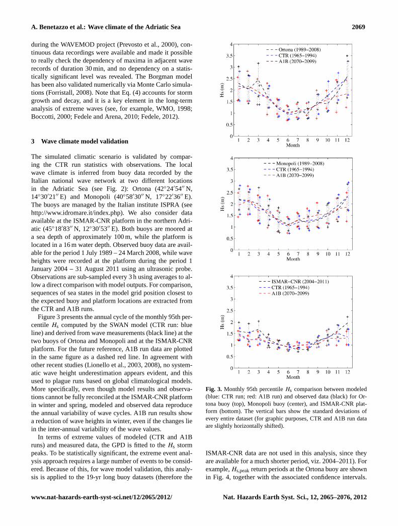
The simulated climatic scenario is validated by compar-ing the CTR run statistics with observations. The localwave climate is inferred from buoy data recorded by theItalian national wave network at two different locationsin the Adriatic Sea (see Fig. 2): Ortona (42◦24′54′′ N,14◦30′21′′ E) and Monopoli (40◦58′30′′ N, 17◦22′36′′ E).The buoys are managed by the Italian institute ISPRA (seehttp://www.idromare.it/index.php). We also consider dataavailable at the ISMAR-CNR platform in the northern Adri-atic (45◦18′83′′ N, 12◦30′53′′ E). Both buoys are moored ata sea depth of approximately 100 m, while the platform islocated in a 16 m water depth. Observed buoy data are avail-able for the period 1 July 1989 – 24 March 2008, while waveheights were recorded at the platform during the period 1January 2004 – 31 August 2011 using an ultrasonic probe.Observations are sub-sampled every 3 h using averages to al-low a direct comparison with model outputs. For comparison,sequences of sea states in the model grid position closest tothe expected buoy and platform locations are extracted fromthe CTR and A1B runs.

Figure 3 presents the annual cycle of the monthly 95th per-centileHs computed by the SWAN model (CTR run: blueline) and derived from wave measurements (black line) at thetwo buoys of Ortona and Monopoli and at the ISMAR-CNRplatform. For the future reference, A1B run data are plottedin the same figure as a dashed red line. In agreement withother recent studies (Lionello et al., 2003, 2008), no system-atic wave height underestimation appears evident, and thisused to plague runs based on global climatological models.More specifically, even though model results and observa-tions cannot be fully reconciled at the ISMAR-CNR platformin winter and spring, modeled and observed data reproducethe annual variability of wave cycles. A1B run results showa reduction of wave heights in winter, even if the changes liein the inter-annual variability of the wave values.

In terms of extreme values of modeled (CTR and A1Bruns) and measured data, the GPD is fitted to theHs stormpeaks. To be statistically significant, the extreme event anal-ysis approach requires a large number of events to be consid-ered. Because of this, for wave model validation, this analy-sis is applied to the 19-yr long buoy datasets (therefore the

Fig. 3. Monthly 95th percentileHs comparison between modeled(blue: CTR run; red: A1B run) and observed data (black) for Or-tona buoy (top), Monopoli buoy (center), and ISMAR-CNR plat-form (bottom). The vertical bars show the standard deviations ofevery entire dataset (for graphic purposes, CTR and A1B run dataare slightly horizontally shifted).

ISMAR-CNR data are not used in this analysis, since theyare available for a much shorter period, viz. 2004–2011). Forexample,Hs,peakreturn periods at the Ortona buoy are shownin Fig. 4, together with the associated confidence intervals.


http://www.idromare.it/index.php


Fig. 4. Return level plot forHs,peakat the Ortona buoy. Empiricaldata (squares) are the POT values for each dataset (black: observed;blue: CTR run; red: A1B run). The return period is calculated inaccordance with Eq. (1), and the observed data confidence intervalis bounded by the gray area. Empirical data are compared to theGPD results (solid lines in figure).

Table 1. Ortona and Monopoli goodness of fit. Obs: buoy data;CTR and A1B: modeled data. R-square: coefficient of determina-tion; RMSE: root-mean-square error.

Parameter GPD-Ortona GPD-Monopoli

R-square (Obs) 0.99 0.99R-square (CTR) 0.99 0.99R-square (A1B) 0.99 0.99RMSE (Obs) 0.06 m 0.05 mRMSE (CTR) 0.04 m 0.06 mRMSE (A1B) 0.04 m 0.05 cm

The fitted distributions of CTR and A1B results show a re-duction of the return values in the future, even if of secondaryorder with respect to the large uncertainty of the extremeevents.

The diagnostic quantile plot (Fig. 5) is considered to es-timate the goodness of the fit to the theoretical GPD. Twofitting parameters are calculated (see Table 1): the R-squareerror and the root-mean-square error (RMSE). The coeffi-cient of determination (R-square) represents the correlationbetween data and fitted model, whereas RMSE accounts forthe error in the regression. From Table 1, note that R-squarevalues are close to 1, meaning that GPD accounts for the datavariance and nicely represents data, having differences in theorder of 0.05 m.

The statistics shown are based on the sea states describedby the significant wave heightHs. This represents the de-gree of sea severity, which relates to the expected maximumwave heightHmax that can occur during a storm. In fact, for

Fig. 5. Quantile plot of the GPD fit at the Ortona buoy. Black: ob-served; blue: CTR run; red: A1B run.

a given storm measured or modeled at a given point in space,Hmax can be estimated ala“Borgman” using Eq. (4) and theRayleigh law for the short-term wave statistics. For example,in the left panel of Fig. 6, we show a scatter plot display-ing theHs,peakvalue of the storm sequence and the associ-ated expected values forHmax. Buoy data show an averageHmax/Hs,peakratio equal to 2.02, while this ratio increases to2.11 for both the CTR and A1B runs. These are typical val-ues of sea surface waves, indicating their quasi-Gaussian sta-tistical nature (see, for example, Boccotti, 2000; Fedele andArena, 2010). TheHmax/Hs,peakratio dependency onHmaxis shown in the right panel of Fig. 6. As expected (Fedeleand Arena, 2010), in Gaussian seas the ratioHmax/Hs,peakre-duces asHmax increases; so rare events haveHmax/Hs,peaksmaller than that of more frequent typical events that canhaveHmax/Hs,peak>2.00. For example, in the observed datathe maximum wave of a storm with a heightHmax = 8.00 moccurs in the strongest sea state of the storm withHs,peak≈ Hmax/2.04≈3.92 m. On the other hand, CTR results yieldthat the same wave height can occur in a sea state withslightly less strength, i.e.Hs,peak≈ Hmax/2.12≈3.77 m. Thisimplies that CTR extremes are more frequent than those ob-served from buoy data.

This small difference can be explained by comparing thetypical shape of wave storms in both the observed and mod-eled data. For example, Fig. 7 illustrates theHs time se-quence of storms computed by the SWAN model forced bythe climatological wind (COSMO-CLM, dashed line) and bythe wind provided by an operational meteorological model(COSMO-I7, dotted line). COSMO-I7 is the Italian ver-sion of the COSMO model, a mesoscale model developedin the framework of the COSMO Consortium (seewww.cosmo-model.org). The typical storm shape is triangular(see, for example, Boccotti, 2000; Fedele and Arena, 2010),


www.cosmo-model.org

www.cosmo-model.org


Fig. 6. Borgman’s analysis of the storms at the Ortona buoy (black: observed; blue: CTR run; red: A1B run). Left: scatter plot of Hmax andHs,peakdata. The linear fitting is superimposed to the collection of scattered points. Right: Hmax/Hs,peakratio with respect to Hmax for eachstorm. The exponential data fitting is superimposed (dashed line).

Fig. 7.A typical wave storm shape from the observedHs data (solidline) and numerical simulations with two different wind forcings(dashed line: COSMO-CLM; dotted line: COSMO-I7).

as confirmed by buoy measurements (see solid line in Fig. 7)and by the wave field output produced by the operationalmeteorological model forcings. On the other hand, to thebest of our knowledge, little attention has been devoted toinvestigate the storm shapes reproduced by climate mod-els, which appear to be mostly parabolic, as clearly seen inFig. 7. For given wave height, parabolic storms yield moreintense extremes than triangular storms, viz. COSMO-CLMforcings can yieldHmax value at moderateHs,peak states,while buoy measurements indicate that to attain the sameHmax requires stronger sea states. In this direction, the pre-dictions of COSMO-CLM yield larger expected maximumwave heights, as depicted in Fig. 6, and modeled wave stormsexperience higherHmax/Hs,peakratios.

4 Present and future wave climate of the Adriatic Sea

In order to assess the wave severity in a climate change per-spective, computedHs are evaluated for the whole Adri-atic Sea at all contiguous model grid locations. Even ifBora and Sirocco wind fields are distinct meteorologicalevents, they are both closely related to cyclonic activity inthe Mediterranean region (see Dorman et al., 2006 and refer-ences therein). Since the paper aims to quantify the expectedfuture changes in the Adriatic Sea wave severity, the resultsare then presented showing the overall wave climate withoutdistinctions between Bora and Sirocco episodes (projectedBora and Sirocco climate conditions can be found in Pasaricand Orlic, 2004).

Based on the wave data analyzed, the Adriatic Sea meansignificant wave height is expected to decrease at a rate ofabout 0.05 % per year, since 1965. Indeed, the two 30-yr longperiods analyzed are long enough to encompass the inter-annual climate modulations, and at the same time they stillsatisfy the hypothesis of stationarity of the wave climate (i.e.,in 30 yr the expected variation is about 1.5 %, less of otherinvolved uncertainties).

Figures 8 and 9 show the average and the maximum sig-nificant wave heightsHs for the present climate (CTR run:1965–1994 period) and for the future scenario (A1B run:2070–2099 period). The CTR run presents higher values, butthe difference with respect to the A1B run is small. The Adri-atic Sea mean difference between A1B and CTR results isin the order of 5 % and 6 %, for the average and maximumHs, respectively. In the future, highest reductions will be ex-pected in the southern and northern Adriatic Sea, while sim-ulations carried out show local increase ofHs levels in thecentral Adriatic Sea. An evaluation of the number of hourswith significant wave height greater than two thresholds (2 mand 5 m in Figs. 10 and 11, respectively) shows that this is



Fig. 8.AverageHs (in meters). Numerical simulations of the present climate (left) and the future scenario (right) are shown.

Fig. 9.MaximumHs (in meters). Numerical simulations of the present climate (left) and the future scenario (right) are shown.

Fig. 10. Yearly average number of hours withHs greater than 2 m. Numerical simulations of the present climate (left) and the futurescenario (right) are shown.

Fig. 11.Yearly average number of hours withHs greater than 5 m. Numerical simulations of the present climate (left) and the future scenario(right) are shown.



Fig. 12.5-yr return significant wave heightHs (in meters). Numerical simulations of the present climate (left) and the future scenario (right)are shown.

Fig. 13.30-yr return significant wave heightHs (in meters). Numerical simulations of the present climate (left) and the future scenario (right)are shown.

generally smaller for the A1B run with respect to the presentclimate.

These conclusions are confirmed by the extreme valueanalysis applied to CTR and A1B datasets. The extreme waveanalysis is based on the POT procedure applied to the two 30-yr long simulated periods (CTR and A1B), fitting theHs,peakvalues to a generalized Pareto distributions to obtain a re-turn period curve. Figures 12 and 13 show the 5-yr (frequentevent) and 30-yr (rare event) return value of the wave heightHs,peak, respectively. Note that the 30-yr return period signif-icant wave height is the wave condition associated with themaximum time interval available in the two datasets CTRand A1B. These two sets of data are assumed to be represen-tative of two stationary climatic conditions: the present andthe expected future.

In accordance with the average wave conditions, the 30-yr returnHs,peakchanges between A1B and CTR runs showmilder waves for the future scenario, with an overall reduc-tion of 5 %. Nevertheless, the simulations performed showa local increase of theHs,peak of approximately 15 % inthe central and southern Adriatic Sea. Wave heights presentlower values in the northern area, with expected reduction of20 % of the 30-yr returnHs,peak. The 5-yr returnHs,peakval-ues show a similar geographical pattern, even if the increase

does not go over 3 %, and the reduction in the northern Adri-atic is limited to 10 %.

Finally, the Borgman model of Eq. (4) permits to estimatethe geographical pattern of the maximum expected waveheight Hmax for a 30-yr long period of sea states. Resultsfor the present (CTR run) and future (A1B run) climates areshown in Fig. 14. In accordance with the pattern of maxi-mum Hs, Adriatic Sea maximum wave heights are locatedin the southern Adriatic Sea for both runs. The predictedfuture changes are small, in the order of 5 %, leaving un-changed the probability of single waves higher than 10 m formost of the Adriatic Sea. The Adriatic Sea future mean ra-tio Hmax/Hs,peakis expected to remain equal to the estimatedactual value of 2.06.

5 Summary and conclusions

The main objective of this study was to assess a possible fu-ture changes in the estimate of the average and extreme seawave states over Adriatic Sea. The procedure was applied totwo 30-yr long periods of wave fields generated by windssimulated by the climatological model COSMO-CLM at 14-km horizontal resolution. In the Adriatic Sea region, whichis characterized by a complex orography, this resolution wasshown to adequately reproduce small spatial scale patterns,



Fig. 14. Borgman’s analysis: Largest expected maximum wave heightHmax in a storm (in meters). Numerical simulations of the presentclimate (left) and the future scenario (right) are shown.

Fig. 15. 30-yr return periodHs,peakbased on the GPD. Pattern oftheHs,peakratio between A1B and CTR results. The black dashedline shows the isoline 1.0.

albeit using wind products from NWP systems (Signell et al.,2005). This approach allowed to provide a high-resolutionmapping of the whole Adriatic Sea, in comparison with pre-vious studies that were employing wind fields at about 50 kmresolution (Lionello et al., 2008, 2012).

The two periods were analyzed for the simulated windconditions of the present-day (CTR run: 1965–1994) and thepredicted (A1B run: 2070–2099) climate conditions, basedon the IPCC A1B emission scenario, which is considereda balance of all energy sources (IPCC, 2007) and is a midline between A2 medium-high emission and B2 medium-lowemission scenarios. The wave simulations were performedwith the SWAN model on the whole Adriatic Sea, imple-mented with a grid resolution of approximately 8 km. Theresults are two 30-yr long time series of significant waveheightsHs for every computational cell, which has shownan overall trend similar results with respect to Lionello etal. (2012) in the northern Adriatic sea, where a reduction ofextreme wave events was envisaged in the future scenariowith respect to the present-day situation.

The comparison between the CTR run results and avail-able field data showed that the modeled wave fields repro-duce to a good extent the seasonality of Adriatic Sea waveclimate, as well as the long-term statistics of wave extremes.Noteworthy, the wave storms resulting from the COSMO-CLM model show a parabolic shape instead of the typicaltriangular form observed from measurements and reportedin literature (see, for example, Boccotti, 2000; Fedele andArena, 2010). This produces small differences in the indi-vidual maxima wave height, here investigated by means ofBorgman’s theory, applied to both modeled and measureddata. Nevertheless, Borgman’s analysis showed that the fu-ture storm shape will remain unchanged, i.e. there is no ten-dency of more intense short-duration wave storm events.

Some statistical parameters were calculated to estimate thedifferences between the current and the future wave climatesimulations. Our analysis shows that, relative to the presentlevel, global Adriatic Sea wave severity is likely to decreaseby 5 % by the end of the 21th century. In particular, followingthe generalized Pareto distribution, the mean Adriatic Sea 30-yr return significant wave height would decrease by 0.28 mbetween 1990s and the 2090s, with a maximum decrease of2.13 m and a maximum increase of 0.85 m.

As expected, the wave height variations will not occur uni-formly across the Adriatic, with some regions experiencinghigher levels of waves and others lower (see for exampleFig. 15). Such variations are due to the variations in the lo-cal wind climate, in accordance with expected changes of thetwo dominant winds in the Adriatic Sea, Bora and Sirocco.Further studies, though, are required to distinguish the Boraand Sirocco roles to produce the local wave climate.

Based on the data herein analyzed, useful suggestions canbe forwarded about the future Adriatic Sea wave climate.When evaluating the impact of climate change on the designof new marine structures and on the safety of existing ones,the design wave based on past events seems to lead to con-servative conditions for a future scenario. The differences,however, between the present and the future wave climate are



small and comparable with the uncertainty that is associatedwith extreme events.

As a final recommendation, it should be noted that whendealing with climate change-related issues, improvements ofthe reliability level of design should require a statistical anal-ysis for extremes that accounts for non-stationary conditions.

Acknowledgements.The Authors gratefully acknowledge the fund-ing from the EC FP7/2007-2013 under grant agreement no. 242284(Project “FIELD AC”). The work was also partially supported bythe FIRB RBFR08D825001 grant (Project “DECALOGO”).

Edited by: U. UlbrichReviewed by: V. Alari, J. Dykes, and another anonymous referee

References

Bellafiore, D., Bucchignani, E., Gualdi, S., Carniel, S., Djurdjevic,V., and Umgiesser, G.: Assessment of meteorological climatemodels as inputs for coastal studies, Ocean Dynam., 62, 555–568, 2012.

Bignami, F., Sciarra, R., Carniel, S., and Santoleri, R.: Variabilityof Adriatic Sea coastal turbid waters from SeaWiFS imagery, J.Geophys. Res., 112, C03S10,doi:10.1029/2006JC003518, 2007.

Bitner-Gregersen, E. M. and Eide, L. I.: DNV Position Paper No.8“Potential Impact of Climate Change on Tanker Design”, 1–20,2011.

Boccotti, P.: Wave Mechanics for Ocean Engineering, Elsevier Sci-ence, Oxford, 496 pp., 2000.

Booij, N., Ris, R., and Holthuijsen, L.: A third-generation wavemodel for coastal regions 1. Model description and validation,J. Geophys. Res., 104, 7649–7666, 1999.

Boldrin, A., Carniel, S., Giani, M., Marini, M., Bernardi Aubry,F., Campanelli A., Grilli, F., and Russo A.: The effect of Borawind on physical and bio-chemical properties of stratified watersin the northern Adriatic, J. Geophys. Res.-Ocean, 114, C08S92,doi:10.1029/2008JC004837, 2009.

Borgman, L. E.: Probabilities for the highest wave in a hurricane, J.Waterway, Port, Coast. Ocean Eng., 99, 185–207, 1973.

Brodtkorb, P. A., Johannesson, P., Lindgren, G., Rychlik, I., Ryden,J., and Sjo, E.: WAFO – a Matlab toolbox for analysis of randomwaves and loads, Proceedings of the 10th International Offshoreand Polar Engineering conference, Seattle, III, 343–350, 2000.

Bucchignani, E., Sanna, A., Gualdi, S., Castellari, S.,and Schiano, P.: Simulation of the climate of the XXcentury in the Alpine space, Nat. Hazards, in press,http://www.springerlink.com/content/c17l0wp74r75677n/,doi:10.1007/s11069-011-9883-8, 2011.

Carniel, S., Warner, J. C., Chiggiato, J., and Sclavo, M.: Investigat-ing the impact of surface wave breaking on modelling the trajec-tories of drifters in the northern Adriatic Sea during a wind-stormevent, Ocean Model., 30, 225–239, 2009.

Carniel, S., Sclavo, M., and Archetti, R.: Towards validating a lastgeneration, integrated wave-current-sediment numerical modelin coastal regions using video measurements, Oceanol. Hydro-biol. Stud., 40, 11–20, 2011.

Coles, S.: An Introduction to Statistical Modeling of Extreme Val-ues, Springer-Verlag, London, 228 pp., 2001.

Dorman, C. E., Carniel, S., Cavaleri, L., Sclavo, M., Chiggiato J.,and others: February 2003 marine atmospheric conditions andthe Bora over the northern Adriatic, J. Geophys. Res.–Ocean,111, C03S03,doi:10.1029/2005JC003134, 2006.

Dykes, J. D., Wang, D. W., and Book, J. W.: An evaluation of a high-resolution operational wave forecasting system in the AdriaticSea, J. Mar. Syst., 78, 255–271, 2006.

Fedele, F.: Space-time extremes of short-crested storm seas, J. Phys.Oceanogr., in press, 2012.

Fedele, F. and Arena, F.: Long-term statistics and extreme waves ofsea storms, J. Phys. Oceanogr., 40, 1106–1117, 2010.

Forristall, G. Z.: How should we combine long and short term waveheight distributions?, Proceedings of the OMAE08 27th Interna-tional Conference on Offshore Mechanics and Arctic Engineer-ing June 15–20, Estoril, Portugal, 2008.

Intergovernmental Panel on Climate Change (IPCC): in: EmissionsScenarios: Special Report of the Intergovernmental Panel on Cli-mate Change, edited by: Nakicenovic, N. and Swart, R., Cam-bridge University Press, 570 pp., 2000.

Intergovernmental Panel on Climate Change (IPCC): Fourth As-sessment Report. Intergovernmental Panel on Climate ChangeSecretariat, Geneva, Switzerland, 2007.

Lionello, P., Elvini, E., and Nizzero, A.: Ocean waves and stormsurges in the Adriatic Sea: intercomparison between the presentand doubled CO2 climate scenarios, Clim. Res., 23, 217–231,2003.

Lionello, P., Cogo, S., Galati, M. B., and Sanna, A.: The Mediter-ranean surface wave climate inferred from future scenario simu-lations, Global Planet. Change 63, 152–162, 2008.

Lionello, P., Galati, M. B., and Elvini, E.: Extreme storm surge andwind wave climate scenario simulations at the Venetian littoral,Phys. Chem. Earth, Parts A/B/C, 40–41, 86–92, 2012.

Martucci, G., Carniel, S., Chiggiato, J., Sclavo, M., Lionello, P., andGalati, M. B.: Statistical trend analysis and extreme distributionof significant wave height from 1958 to 1999 – an application tothe Italian Seas, Ocean Sci., 6, 525–538,doi:10.5194/os-6-525-2010, 2010.

May, W. and Roeckner, E.: A time-slice experiment with theECHAM4 AGCM at high resolution: the impact of horizontalresolution on annual mean climate change, Clim. Dynam., 17,407–420, 2001.

Pal, J. S., Small, E. E., and Eltahir, E. A. B.: Simulation of regional-scale water and energy budgets: Representation of subgrid cloudand precipitation processes within RegCM, J. Geophys. Res.-Atmos., 105, 29579–29594, 2000.

Pasaric, M. and Orlic, M.,: Meteorological forcing of the Adriatic– present vs. projected climate conditions, Geofizika, 21, 69–87,2004.

Prevosto, M., Krogstad, H. E., and Robin, A.: Probability distri-butions for maximum wave and crest heights, Coast. Eng., 40,329–360, 2000.

Raisanen, J., Hansson, U., Ullerstig, A., Doscher, R., Graham, L. P.,Jones, C., Meier, H. E. M, Samuelsson, P., and Willen, U.: Euro-pean climate in the late twenty-first century: regional simulationswith two driving global models and two forcing scenarios, Clim.Dynam., 22, 13–31, 2004.

Rockel, B. and Woth, K.: Extremes of near-surface wind speed overEurope and their future changes as estimated from an ensembleof RCM simulations, Climatic Change, 81, 267–280, 2007.


http://dx.doi.org/10.1029/2006JC003518

http://dx.doi.org/10.1029/2008JC004837

http://www.springerlink.com/content/c17l0wp74r75677n/

http://dx.doi.org/10.1007/s11069-011-9883-8

http://dx.doi.org/10.1029/2005JC003134

http://dx.doi.org/10.5194/os-6-525-2010

http://dx.doi.org/10.5194/os-6-525-2010


Rockel, B., Will, A., and Hense, A.: The regional Climate ModelCOSMO-CLM (CCLM), Meteorol. Z., 17, 347–348, 2008.

Sclavo, M., Liberatore, G., and Ridolfo, R.: Waves in front of theVenetian littoral, Il Nuovo Cimento, 19, 125–150, 1996.

Shao, Y. and Hahn, M. G.: Maximum product of spacings method:A unified formulation with illustration of strong consistency, Illi-nois J. Math., 43, 489–499, 1999.

Signell, R. P., Carniel, S., Cavaleri, L., Chiggiato, J., Doyle, J.,Pullen, J., and Sclavo, M.: Assessment of wind quality foroceanographic modeling in semi-enclosed basins, J. Mar. Syst.,53, 217–233, 2005.

Steppeler, J., Doms, G., Schattler, U., Bitzer, H. W., Gassmann, A.,Damrath, U., and Gregoric, G.: Meso-gamma scale forecasts us-ing nonhydrostatic model LM, Meteorol. Atmos. Phys., 82, 75–96, 2003.

Tayfun, M. A. and Fedele, F.: Wave-height distributions and nonlin-ear effects, Ocean Engineering, 34, 1631–1649, 2007.

Vinoth, J. and Young, I. R.: Global estimates of extreme wind speedand wave height, J. Climate, 24, 1647–1665, 2011.

WMO (World Meteorological Organization): Guide to Wave Anal-ysis and Forecasting, second edition, 159 pp., 1998.


wave climate of the adriatic sea: a future scenario simulation

Documents