Wave propagation in heterogeneous porous media

formulated in the frequency-space domain using a

discontinuous Galerkin method

Bastien Dupuy∗, Louis De Barros†, Stephane Garambois∗ and Jean Virieux∗

∗Laboratoire de Geophysique Interne et Tectonophysique, Universite Joseph Fourier,

CNRS, Grenoble, France. E-mail: Bastien.Dupuy@obs.ujf-grenoble.fr.

†University College of Dublin, Ireland.

(March 7, 2011)

Running head: Frequency-space approach

ABSTRACT

Biphasic media with a dynamic interaction between fluid and solid phases must be taken

into account to accurately describe seismic wave amplitudes in subsurface and reservoir

geophysical applications. Consequently, the modelling of the wave propagation in heterege-

neous porous media, which includes the frequency-dependent phenomena of the fluid-solid

interaction, is considered for 2D geometries. From the Biot-Gassmann theory, we deduce the

discrete linear system in the frequency domain for a discontinuous finite element method,

known as the nodal discontinuous Galerkin method. We show that solving this system in the

frequency domain allows accurate modelling of the Biot wave in the diffusive/propagative

regimes, enhancing the importance of frequency effects. Because we must consider finite

numerical models, we implement perfectly matched layer techniques and we show that

waves are efficiently absorbed at the model boundaries. We find that the discretization

of the medium should follow the same rules as in the elastodynamic case, that is 10 grids

1

per minimum wavelength for a P0 interpolation order. The grid spreading of the sources,

which can be stresses or forces applied either on the solid or fluid phases, does not show

any additional difficulties compared to the elastic problem. For a flat interface separating

two media, we compare the numerical solution and a semi-analytical solution obtained by

a reflectivity method in the three different regimes where the Biot wave is propagative,

diffusive/propagative and diffusive. In all cases, fluid-solid interactions are accurately re-

constructed, showing that attenuation and dispersion of the waves are correctly accounted

for. After this validation in layered media, we illustrate the capacities of modelling complex

wave propagation in laterally heterogeneous porous medium related to a steam injection in

a sand reservoir and we show the seismic response associated to a fluid substitution.

2

INTRODUCTION

For many geophysical applications such as those related to reservoir issues (oil, gas or

CO2 storage) or geotechnical problems (slope stability, water resources), it is essential to

consider a biphasic material marked by a dynamic interaction between fluid and solid phases

in order to accurately describe seismic wave amplitudes. Since pioneer works of Biot (1956)

and Gassmann (1951) on poroelastodynamics, analytical and numerical methods have been

developped for the simulation of wave propagation in biphasic porous media.

For simple cases, analytic solutions are available as those proposed by Burridge and

Vargas (1979) who have identified clearly the three waves predicted by the work by Biot

(1956) or those by Boutin et al. (1987) who have computed analytical Green functions in

a stratified saturated porous medium. An experimental validation has been carried out

by Plona (1980), who was the first to observe the Biot slow wave. Reflectivity methods

have solved these equations in simple 3D stratified media (Stern et al., 2003; De Barros

and Dietrich, 2008) and permitted the study of their electrokinetic coupling (Haartsen and

Pride, 1997; Garambois and Dietrich, 2002) and the necessity to take into account the Biot

slow wave for seismo-electromagnetic characterisation (Pride and Garambois, 2002, 2005).

Considering lateral heterogeneities requires numerical methods based on volumetric dis-

cretization for solving equations of poroelastodynamics. The most popular of these tech-

niques are the finite-difference methods (FDM) as used for example by Dai et al. (1995)

who observed the ”slow” P-wave influence on attenuation in synthetic and real data. More

recently, Wenzlau and Muller (2009) used velocity-stress finite-difference method to study

fluid diffusion processes in planar cracks, illustrating limitations of FDM to rather simple

geometries. Using the accurate spectral element method (SEM), Morency and Tromp (2008)

3

investigated the validity of Biot theory in media with porosity gradients while Morency et al.

(2009) have performed the analysis of finite-frequency kernels needed for the reconstruction

of medium parameters. Similarly, the discontinuous Galerkin method (DGM) in time do-

main (De la Puente et al., 2008) has been successfully used to compute wave propagation in

saturated anisotropic porous media with complex discontinuity geometries. In their review,

Carcione et al. (2010) sum up the approaches previously described.

Most of these numerical approaches in the time domain assume some simplifications

in the interaction between solid and fluid phases, called low frequency approximation in

our presentation of the Biot theory. Masson and Pride (2010) have shown that consider-

ing effects of all frequencies and not only low frequency approximation is essential for a

correct estimation of the Biot wave amplitude. Therefore, if we are interested to compute

the entire wave signal taking into account Biot wave and P & S waves, we should take into

account dispersive effects related to the frequency dependence of poroelastic parameters.

Moreover, for superficial saturated media where fluid/solid interactions are prevailing, the

low frequency approximation is not valid anymore regardless of the Biot wave regime. Con-

sequently, solving poroelastodynamics in the frequency domain will improve our description

of the physical behaviour between solid and fluid phases.

From the numerical point of view, these numerical methods in the time domain share

the difficult issue of having to use very small time steps when considering a viscous fluid.

Carcione (1996) has shown how to turn around this difficulty by using a partition method

(Carcione and Goode, 1995) although it requires a local eigenvalue decomposition: the

partial differential system to be solved is decomposed into two sets, one stiff and the other

non-stiff. The first one is solved implicitly while the other one is solved explicitly using a

Runge-Kutta integration with CFL condition related to wave propagation characteristics

4

in solid media. Recently, Masson and Pride (2010) have underlined that the CFL stability

condition is strongly related to the values of the fluid viscocity. They have shown that, for

typical values of saturated media, the limitation is not so drastic when adequate convolution

is performed to consider frequency effects.

The formulation of the diffusion/propagation problem in the frequency domain will

avoid the difficult issue of small time integration steps at the expense of solving a sparse

linear system. This approach has been proposed by many authors for visco-elastodynamics

problems (Stekl and Pratt, 1998; Hustedt et al., 2004; Plessix, 2007; Brossier et al., 2008b).

This is an efficient approach when considering full waveform inversion if we are able to use

a direct solver approach: we can efficiently solve the forward problem for many sources,

a linear system with multiple right-hand-sides (Pratt et al., 1998; Plessix, 2006; Brossier

et al., 2009), thanks to the LU decomposition performed once for the medium (this step is

sometimes called the factorisation step). The solving step which comprises in an efficient

downward and upward substitution for getting the solution is performed for each source.

Here, we investigate the feasibility of the 2D wave propagation modelling for porous me-

dia in the frequency domain while including complete dispersion and diffusion description,

thanks to the frequency formulation. We shall consider a discontinuous Galerkin method

(DGM) which has been shown to be quite efficient for 2D geometries with complex interface

geometries (Brossier et al., 2008b).

First, we present the description of biphasic porous medium as well as the Biot theory

of poroelastodynamics. Then, we outline the numerical steps of the DGM constructing the

linear system which can be solved by a direct solver for 2D geometries. We compare on

some simple examples numerical DGM results with analytical solutions and semi-analytical

5

results based on boundary integral equations. Finally, we show an illustration of wave

propagation in a laterally variable medium before outlining perspectives and conclusions.

POROELASTIC GOVERNING EQUATIONS

The introduction of poroelastodynamics is related to strong amplitude variations one can

observe in practice especially for shallow seismic experiments. In this work, we focus our

investigation only on porous elastodynamics for simplicity. Extension for including at-

tenuation and viscous mechanisms which also control the amplitude variations are then

straightforward when considering frequency formulation, an advantage we should keep in

mind, leading to visco-poroelastodynamics to be considered for real applications. Moreover,

the frequency formulation can be easily adapted to take into account more complex phys-

ical phenomena such as partial saturation (White, 1975; Dutta and Ode, 1979) or double

porosity (Pride and Berryman, 2003).

Porous media homogenisation

The description of porous media requires an homogenisation approach of both fluid and

solid phases in order to deduce an equivalent medium (Burridge and Vargas, 1979). The

porosity φ = VV /VT , which is the ratio between void and total volumes, defines respective

proportions of fluid and solid phases.

The fluid and associated flows through the solid matrix, is described by an uncompress-

ibility modulus Kf , a density ρf and a viscosity η. A non-viscous fluid has a viscosity η

equal to zero. The viscosity can be formulated with the intrinsic permeability k0 intro-

duced in the Darcy’s law. Auriault et al. (1985) and Johnson et al. (1987) have generalised

6

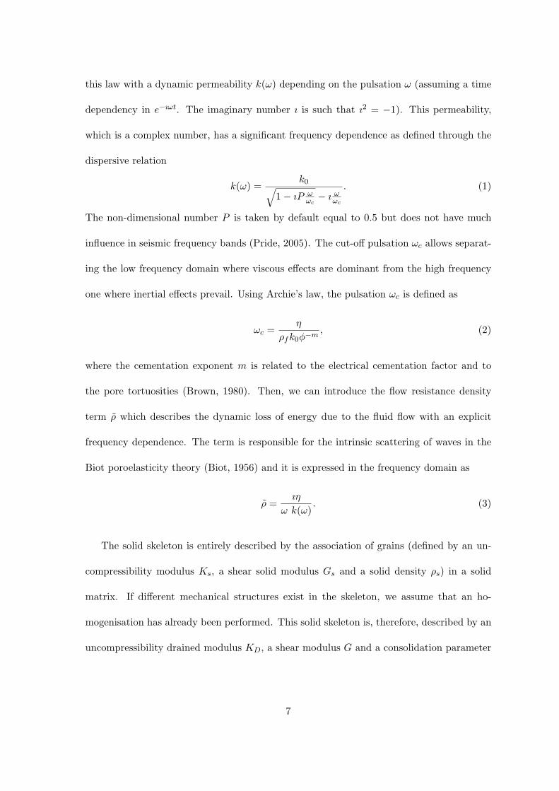
this law with a dynamic permeability k(ω) depending on the pulsation ω (assuming a time

dependency in e−ıωt. The imaginary number ı is such that ı2 = −1). This permeability,

which is a complex number, has a significant frequency dependence as defined through the

dispersive relation

k(ω) =k0√

1− ıP ωωc

− ı ωωc

. (1)

The non-dimensional number P is taken by default equal to 0.5 but does not have much

influence in seismic frequency bands (Pride, 2005). The cut-off pulsation ωc allows separat-

ing the low frequency domain where viscous effects are dominant from the high frequency

one where inertial effects prevail. Using Archie’s law, the pulsation ωc is defined as

ωc =η

ρfk0φ−m, (2)

where the cementation exponent m is related to the electrical cementation factor and to

the pore tortuosities (Brown, 1980). Then, we can introduce the flow resistance density

term ρ which describes the dynamic loss of energy due to the fluid flow with an explicit

frequency dependence. The term is responsible for the intrinsic scattering of waves in the

Biot poroelasticity theory (Biot, 1956) and it is expressed in the frequency domain as

ρ =ıη

ω k(ω). (3)

The solid skeleton is entirely described by the association of grains (defined by an un-

compressibility modulus Ks, a shear solid modulus Gs and a solid density ρs) in a solid

matrix. If different mechanical structures exist in the skeleton, we assume that an ho-

mogenisation has already been performed. This solid skeleton is, therefore, described by an

uncompressibility drained modulus KD, a shear modulus G and a consolidation parameter

7

cs. With the help of the porosity, empirical formulae (Pride, 2005) defined as

KD = Ks1− φ

1 + cs φ,

G = Gs1− φ

1 + 32 cs φ

(4)

link mineral properties to the parameters that characterize the skeleton itself. The con-

solidation parameter cs and the porosity φ are key ingredients for upscaling constitutive

parameters.

Homogenisation of the solid and fluid phases leads to the following definitions of various

mechanical quantities required for dynamic mechanical modelling. The density of the porous

medium is the arithmetic mean of fluid and solid phases weighted by their own volumes via

the porosity, such that

ρ = (1− φ) ρs + φ ρf . (5)

The introduction of the undrained uncompressibility modulus KU , the Biot C modulus and

the fluid storage coefficient M allows the explicit description of the homogenised porous

medium through the Gassmann relations (Gassmann, 1951). Relationships between coeffi-

cients KU , C and M and the modulus functions of KD, Ks, Kf and φ are given by

KU =φ KD + (1− (1 + φ) KD/Ks) Kf

φ (1 + ∆),

C =(1−KD/Ks) Kf

φ (1 + ∆), (6)

M =Kf

φ (1 + ∆),

with the additional expression

∆ =1− φ

φ

Kf

Ks

(1− KD

(1− φ) Ks

). (7)

The shear modulus of the porous medium G is independent of the fluid characteristics and,

8

therefore, equal to the shear modulus of the drained solid skeleton through the relation 4

where only the porosity φ and the consolidation parameter cs are involved.

Biot theory

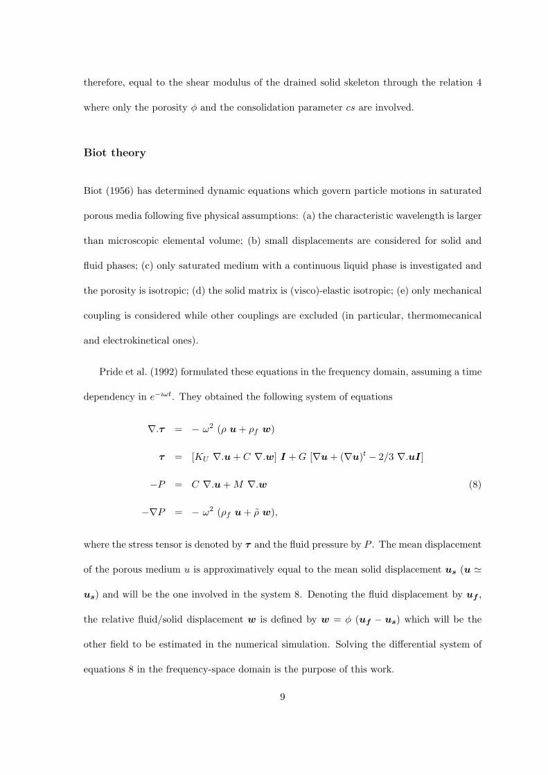
Biot (1956) has determined dynamic equations which govern particle motions in saturated

porous media following five physical assumptions: (a) the characteristic wavelength is larger

than microscopic elemental volume; (b) small displacements are considered for solid and

fluid phases; (c) only saturated medium with a continuous liquid phase is investigated and

the porosity is isotropic; (d) the solid matrix is (visco)-elastic isotropic; (e) only mechanical

coupling is considered while other couplings are excluded (in particular, thermomecanical

and electrokinetical ones).

Pride et al. (1992) formulated these equations in the frequency domain, assuming a time

dependency in e−ıωt. They obtained the following system of equations

∇.τ = − ω2 (ρ u+ ρf w)

τ = [KU ∇.u+ C ∇.w] I +G [∇u+ (∇u)t − 2/3 ∇.uI]

−P = C ∇.u+M ∇.w (8)

−∇P = − ω2 (ρf u+ ρ w),

where the stress tensor is denoted by τ and the fluid pressure by P . The mean displacement

of the porous medium u is approximatively equal to the mean solid displacement us (u '

us) and will be the one involved in the system 8. Denoting the fluid displacement by uf ,

the relative fluid/solid displacement w is defined by w = φ (uf − us) which will be the

other field to be estimated in the numerical simulation. Solving the differential system of

equations 8 in the frequency-space domain is the purpose of this work.

9

Wave slownesses

Biot theory (system 8) predicts three wave types: a compressional and a shear waves similar

to those propagating inside an elastic body and a slow compressional wave, called Biot wave,

which is strongly diffusive and attenuated at low frequencies. This Biot wave behaves as

either a diffusive signal or a propagative wave depending on the frequency content of the

source with respect to the cut-off pulsation or characteristic frequency, as defined in equation

2. The slowness of the shear wave is given by the following equation (Pride, 2005)

s2S =ρ− ρ2f/ρ

G, (9)

while slownesses of compressional waves, the P and Biot waves, are given by

s2P = γ −

√γ2 −

4(ρρ− ρ2f )

HM − C2, s2Biot = γ +

√γ2 −

4(ρρ− ρ2f )

HM − C2(10)

where γ and H terms are

γ =ρM + ρH − 2ρfC

HM − C2, H = KU +

4

3G . (11)

Parameters homogenisation

The macroscale physical parameters which are needed in the poroelastodynamic equations

(system 8) are

• four mechanical parameters: uncompressibility modulus KU and shear modulus G of

the porous medium, the Biot C modulus which describes fluid/solid coupling and the

storage coefficient M for the fluid behaviour.

• three density terms: fluid density ρf , mean density ρ and the complex frequency-

dependent flow resistance term ρ.

10

These parameters are deduced from physical input parameters which are the fluid ones

(Kf , η, ρf ), the mineral ones (Ks, Gs, ρs) and those related to the skeleton arrangement

as the consolidation cs and the cementation exponent m, the porosity φ and hydraulic

permeability k0 (see Table 1 for typical values). Relationships (equations 3, 4, 5 and 6)

between these input parameters and the poroelastodynamic parameters needed for the

forward modelling are explicit with singularities we shall discuss. For a frequency of 200 Hz

and, therefore, a pulsation of 1260 rad/sec, Figure 1 presents the variations with respect to

the porosity of the three density terms (top panel) and the four mechanical moduli (bottom

panel). We observe a linear evolution of the mean density ρ with respect to the porosity

φ. It is equal to the solid density for φ = 0 and to the fluid density for φ = 1. As the

considered medium is consolidated, all the mechanical parameters decrease with increasing

porosity which corresponds to an increasing influence of the fluid. These parameters and

the average density vary inside a bounded interval from the pure solid (φ = 0) to the pure

fluid (φ = 1), except for two parameters. The flow resistance term ρ and the parameter M

are singular when the porosity tends towards zero. In association with these singularities,

the relative fluid/solid displacement vector (w = φ (uf − us)) decreases to zero as well

and, therefore, the terms C ∇.u, M ∇.w and ρ w in the differential equations vanish when

computing the solution. Hence, we can retrieve exact elastodynamic equations by setting

M = ρ = 0 for the specific case φ = 0. On the other hand, when the porosity tends

towards one, the medium is a complete fluid and so the flow resistance term ρ, related to

the interaction between the fluid and the solid, reaches a minimum because there is no

more viscous interaction between fluid and solid phases. We end up by modelling wave

propagation for the elastic monophasic case using this poroelastic formulation although

this is not very efficient in terms of computer resources. We verified that small values of

11

φ = 10−3 do not trigger any numerical instabilities in the direct solver we are using and

provide nearly identical results as in the solid monophasic case at frequencies we usually

consider in our different synthetic modellings.

DISCONTINUOUS GALERKIN METHOD IN FREQUENCY-SPACE

DOMAIN

Frequency-space approach

We solve partial differential equations in the frequency-space domain: volumetric methods

have been extensively developed in the time-space domain while boundary integral equations

through a spectral formulation are more often expressed in the frequency-wavenumber do-

main. Solving in the frequency-space domain has started to be considered intensively when

tackling the full waveform inversion as thousands of forward problems are required for re-

covering the medium properties. We now introduce a discontinuous finite element method

called Discontinuous Galerkin Method (DGM) in the frequency domain. This method is

found to be quite accurate especially when considering complex interface geometries and

topographies. Moreover, discontinuous conditions also allow considering fluid/solid inter-

faces. The advantages found for the elastic formulation should be valid for the poroelastic

approach. For a more detailed description of the discontinuous Galerkin method, we refer to

the book of Hesthaven and Warburton (2008) and the work of Brossier (2010) and Brossier

et al. (2010) for the elastodynamic case. The spatial discretization is based on triangular

meshes with nodal interpolation inside each cell of the mesh and transforms differential

equations into a linear system to be solved.

12

Discontinuous Galerkin formulation

In 2D heterogeneous discrete domains, we consider the discrete velocity fields (ux and uz)

corresponding to the discretization of the time derivative of the mean porous displacement

u and the discrete relative velocity fields (wx and wz) corresponding to the discretization

of the time derivative of the relative fluid/solid displacement w. Three discrete stress

components (σxx, σzz, σxz) are applied to the mean porous medium while only a discrete

pressure field P is considered inside the fluid. This leads to eight unknowns to be estimated

in each cell of the mesh while one has five unknowns when considering only a solid elastic

medium. We apply the following transformation for the stress/pressure components tensor

T t = (T1, T2, T3, T4) =

(σxx + σzz

2,σxx − σzz

2, σxz , − P

). (12)

Consequently, we have the expression of pressure through the component T1 in the mean

porous medium (confining pressure) and through the component T4 in the fluid (interstitial

pressure). We consider as well the following buoyancy terms deduced from the standard

density terms,

ρ1 =ρ2fρ

− ρ , ρ2 =ρρ

ρf− ρf , ρ3 =

ρ2fρ

− ρ, (13)

13

which are involved in the following differential system we deduce from the system 8

iω ux =1

ρ1

(sx

∂(T1 + T2)

∂x+ sz

∂T3

∂z− Fσx

)+

1

ρ2

(sx

∂T4

∂x+ FPx

),

iω uz =1

ρ1

(sz

∂(T1 + T2)

∂z+ sx

∂T3

∂x− Fσz

)+

1

ρ2

(sz

∂T4

∂z+ FPz

),

iω wx =1

ρ2

(sx

∂(T1 + T2)

∂x+ sz

∂T3

∂z− Fσx

)+

1

ρ3

(sx

∂T4

∂x+ FPx

),

iω wz =1

ρ2

(sz

∂(T1 + T2)

∂z+ sx

∂T3

∂x− Fσz

)+

1

ρ3

(sz

∂T4

∂z+ FPz

),

−iω T1 = (KU +G)

(s′x

∂ux∂x

+ s′z∂uz∂z

)+ C

(s′x

∂wx

∂x+ s′z

∂wz

∂z

)− iω T 0

1 ,

−iω T2 = G

(s′x

∂ux∂x

− s′z∂uz∂z

)− iω T 0

2 ,

−iω T3 = G

(s′z

∂ux∂z

+ s′x∂uz∂x

)− iω T 0

3 ,

−iω T4 = C

(s′x

∂ux∂x

+ s′z∂uz∂z

)+M

(s′x

∂wx

∂x+ s′z

∂wz

∂z

)− iω T 0

4 . (14)

We consider absorbing conditions (i.e. the functions si and s′i) at the edges of the limited nu-

merical domain through the Perfectly Matched Layer (PML) formulation (Berenger, 1994).

Functions sx and sz for velocity equations and s′x and s′z for stress equations are equal to

one inside the medium and decay slowly inside PML regions. Source terms are point forces

(Fσx , Fσz , FPx , FPz) applied on the mean porous medium or on the fluid phase. We may

consider as well external applied stresses (T 01 , T

02 , T

03 , T

04 ) on the mean porous medium or on

the fluid phase. Based on a variational approach, a surface integration in 2D is performed

inside each cell of the mesh sampling the medium. For simplicity sake, a P0 approxima-

tion, i.e. constant quantities inside each cell i, is considered for unknown field components

in the following description although we also implement higher-order (first-order P1 and

second-order P2) lagrangian nodal interpolation inside each cell in the computer code we

have developed. Using the Green’s theorem, the system 14 can be recast into a discrete

form considering four flux vectors (G1, G2, G3 and G4) depending on stresses for velocity

estimation and five flux vectors (H1, H2, H3, H4 and H5) depending on velocities for stress

14

estimation, giving us the discrete linear system

iωAi Vi − 1

ρ1i

∑j∈∂Ki

lijG1ij −

1

ρ2i

∑j∈∂Ki

lijG2ij −

1

ρ2i

∑j∈∂Ki

lijG3ij

− 1

ρ4i

∑j∈∂Ki

lijG4ij = AiFi ,

−iωAi Ti − (KUi +Gi)∑

j∈∂Ki

lijH1ij − Ci

∑j∈∂Ki

lijH2ij −Gi

∑j∈∂Ki

lijH3ij

− Ci

∑j∈∂Ki

lijH4ij −Mi

∑j∈∂Ki

lijH5ij = − iωAi T

0i , (15)

where the surface of the cell i is denoted by Ai. The index j denotes the three neighbours of

the cell i. The length of the boundaries between the current cell i and its neighbours is called

lij and fluxes are computed across these boundaries. Medium parameters are assumed to be

constant inside each cell, regardless of the order we use for velocity and stress components.

Source terms (external forces Fi and stresses T 0i ) can be merged into a source vector b,

which is the right-hand side (RHS) of the system 15. Centered fluxes of stress components

Gαij and velocity components Hβ

ij are expressed as

Gαij =

∑k∈(x,z)

nijkMβk

skiTi + skjTj

2,

Hβij =

∑k∈(x,z)

nijkNαk

s′kiVi + s′kjVj

2, (16)

α ∈ (1; 4) , β ∈ (1; 5) , k ∈ (x, z) ,

where projection matrices Mβx , M

βz , N

αx and Nα

z are given in appendix A. The vector

nijk is the normal vector of each side of the current cell i oriented toward the neighbour

cell j. Combining unknowns of the cell i and the three neighbouring cells j allows the

construction of the sparse matrix of the left-hand side (LHS) of the linear system 15. We

can gather the unknowns of each cell (Ti, Vi) of the mesh in a global vector x we need

to estimate. We end up with a linear sparse matrix system A.x = b. The number of

unknowns (eight for poroelastodynamics with respect to five for elastodynamics) increases

15

the fill-in of the sparse impedance matrix from 41 non-zero terms in elastodynamics to 104

in poroelastodynamics for P0 order. The complex impedance matrix A can be decomposed

through a LU transformation (Amestoy et al., 2006) only once, making very attractive

solving the forward problem in the frequency domain when considering multi-sources as

needed for seismic imaging. The impedance matrix is not symmetrical because of PML

boundary conditions.

NUMERICAL ASPECTS

Four main issues should be considered when solving the linear system we have built for each

frequency. Firstly, the meshing should be considered small enough to accurately model

continuous fields by discrete fields. Then, as the numerical model is always finite, we

must device a technique to absorb waves when they hit the computational boundaries of

the model. Moreover, we compare the computational costs between this approach and

elastic simulations. Finally, we end this section underlining the implementation of external

excitation sources.

Meshing strategy

We use triangular cells to sample spatially the medium as allowed by the discontinuous

Galerkin method. Each triangular element can have its own interpolation order, leading

to the p-adaptivity of the method. The P0 order consists of assuming constant values

of the fields inside each cell, while the P1 order assumes a linear interpolation and the

P2 one a quadratic interpolation. Remaki (2000) and Brossier et al. (2008b) have shown

that regular meshes are required when considering P0 order to avoid kinematic shifts in

16

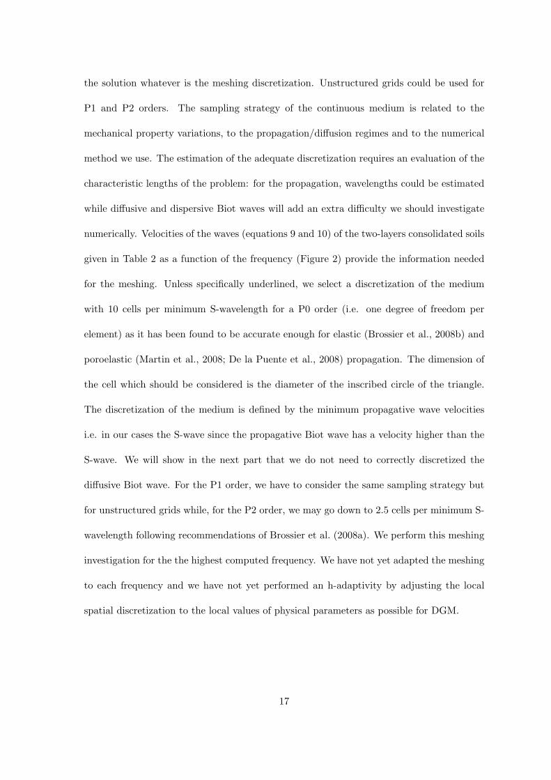
the solution whatever is the meshing discretization. Unstructured grids could be used for

P1 and P2 orders. The sampling strategy of the continuous medium is related to the

mechanical property variations, to the propagation/diffusion regimes and to the numerical

method we use. The estimation of the adequate discretization requires an evaluation of the

characteristic lengths of the problem: for the propagation, wavelengths could be estimated

while diffusive and dispersive Biot waves will add an extra difficulty we should investigate

numerically. Velocities of the waves (equations 9 and 10) of the two-layers consolidated soils

given in Table 2 as a function of the frequency (Figure 2) provide the information needed

for the meshing. Unless specifically underlined, we select a discretization of the medium

with 10 cells per minimum S-wavelength for a P0 order (i.e. one degree of freedom per

element) as it has been found to be accurate enough for elastic (Brossier et al., 2008b) and

poroelastic (Martin et al., 2008; De la Puente et al., 2008) propagation. The dimension of

the cell which should be considered is the diameter of the inscribed circle of the triangle.

The discretization of the medium is defined by the minimum propagative wave velocities

i.e. in our cases the S-wave since the propagative Biot wave has a velocity higher than the

S-wave. We will show in the next part that we do not need to correctly discretized the

diffusive Biot wave. For the P1 order, we have to consider the same sampling strategy but

for unstructured grids while, for the P2 order, we may go down to 2.5 cells per minimum S-

wavelength following recommendations of Brossier et al. (2008a). We perform this meshing

investigation for the the highest computed frequency. We have not yet adapted the meshing

to each frequency and we have not yet performed an h-adaptivity by adjusting the local

spatial discretization to the local values of physical parameters as possible for DGM.

17

Absorbing boundary conditions: Perfectly Matched Layers (PML)

Firstly introduced by Berenger (1994) for electromagnetism, PML have been extensively

applied by different authors to various problems. More specifically, Brossier et al. (2008a)

and Etienne et al. (2009) have analysed them in 2D and 3D nodal DGM elastodynamic

equations using the same formulation we consider in this work. We need a specific meshing

strategy inside the PML layer such that continuous lines parallel to the numerical boundary

exist as we enter deeper in the PML zone because only the flux components perpendicular to

PML boundaries are efficiently damped (Brossier et al., 2008a). In the corners, the meshing

tentatively adapt its strategy to two contrary conditions (see Figure 3). The application of

these contrains in the mesh design of triangles is supported by the software we are using

(TRIANGLE by Shewchuk (1996)). Moreover, damping functions, as proposed by Drossaert

and Giannopoulos (2007), seem to be the most efficient ones. By considering the variable r

as being either x or z, these functions are expressed as

sr =1

κr + iγr,

γr(l) = B

(1− cos

(lπ

2 lPML

)), κr(l) = 1 + C

(1− cos

(lπ

2 lPML

)), (17)

with the thickness of PML area denoted by lPML and l is the distance between the cell and

the edge of the PML. We look for the values of the factors B and C which are optimal for

the most efficient absorption of waves inside the PML layer.

In this aim, we consider an homogeneous model of 70 m by 70 m square which should

be considered as infinite. PML zones add an extra 2 ∗ 5 m length in both directions. An

explosive source is considered at the position x = 10 m and z = 10 m of the porous

medium (see the top panel of Figure 4). The source time function is a Ricker signal with

a central frequency of 200 Hz. Table 1 provides the physical values for our simulations.

18

The parameters lead to a cut-off frequency equal to 6400 Hz and as the frequency band

(1− 600 Hz) is lower than fc, the Biot wave has a diffusive regime.

The DGM in space-frequency domain computes the stationary field for each selected

frequency. We consider 50 discrete frequencies between 1 and 600 Hz. The frequency

range up to fmax = 600 Hz induces a minimum S-wavelength λmin = VS/fmax = 1.43 m.

Therefore, cell size should be smaller than 0.14 m in a regular mesh for P0 order. For P1

order, we use the same discretization for an unstructured grid while, for P2 order case, we

can consider a cell size around 0.57 m. We do not link the discretization of the medium to

the ”wavelength” of the Biot wave as it is strongly attenuated and highly dispersive in this

case. We have found that efficient absorption is obtained with same values as those used

for the elastodynamic modelling, i.e. B = 25 and C = 2 with the thickness of 5 m for the

PML layers we have selected.

Actually, the PML conditions absorb indeed 99 % of the wave energy. If higher ab-

sorption is required for specific applications, one can extend the PML thickness increasing

significantly the computational cost, improving the PML efficiency by one order of magni-

tude, as we have checked with a PML thickness of 10 m.

As the simulation is carried out in the frequency domain, the effect of PML conditions

is felt at any time when we go back to the time domain by an inverse Fourier transform.

We check that similar values provide efficient absorption for a propagative/diffusive inter-

mediate Biot regime (corresponding to a cut-off frequency fc = 64 Hz and a permeability

k0 = 10−9 m2) as well as for a propagative Biot regime (corresponding to a cut-off frequency

fc = 0.64 Hz and a fluid viscosity η = 10−7 Pa.s). Of course, as the medium becomes less

permeable, the field w becomes weaker with respect to the field u and parasite reflections

19

from the field u negligible when considering only this field might introduce noises in the

field w. In our different examples, we find that this problem is not too drastic as long

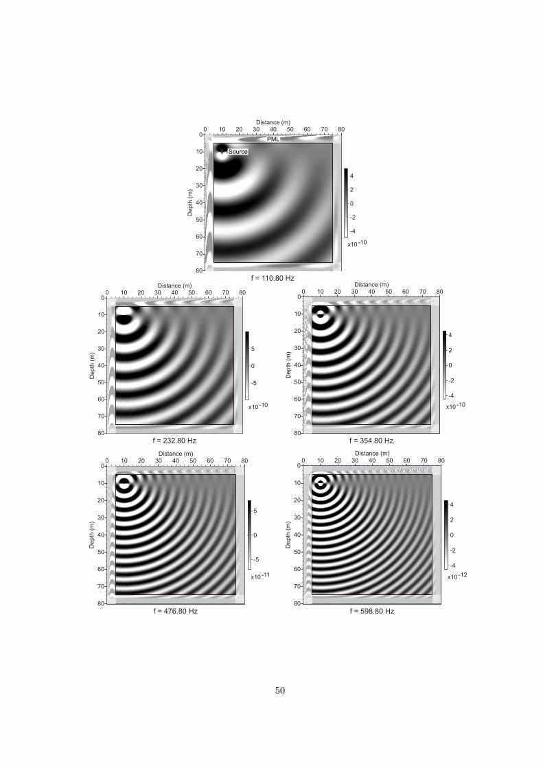
as we consider the above parameters for the PML absorption. Figure 4 shows frequency

waveform maps for the uz component at different frequencies. Similar behaviours are ob-

tained for other components. Putting the source nearby a corner increases the difficulty of

this numerical test with grazing parasite strong reflections on numerical boundaries. One

can see the efficient damping of waves inside the PML layers. Performing an inverse fast

Fourier transform gives us the reconstructed snapshot in the time domain (Figure 5) where

the efficiency of PML conditions is again illustrated.

Computational cost estimation

In Table 3, we compare time and memory of LU factorisation for elastic and poroelastic

DGM modelling with P0, P1 and P2 orders. The fill-in increases by a factor of 104/41 ' 2.5

which is the ratio of non-zero elements between the elastic and poroelastic matrices. For

a standard simulation, computation times and memory are provided in Table 3 for both

elastic and poroelastic cases. We observe a factor of 3 to 5 for time and memory resources

in order to solve the linear system through the LU decomposition (we use the direct solver

MUMPS (Amestoy et al., 2000)) in coherence with the increase of the theoretical fill-in.

For 2D geometries, extension towards poroelastodynamics is still manageable with available

computer resources for present-day clusters but, for high-orders interpolations (P1 and P2

orders), we have to limit our model sizes because of memory limitations. Consequently, our

simulations are performed using the P0 order. The P1 and P2 orders can be used in local

areas to enhance solution precision as, for example, along irregular interfaces or in near-field

source zones. Despite the different orders of magnitude in the values of the parameters and

20

the field unknowns, single precision storage for complex numbers are found to be enough

for the different simulations we present here.

Source implementation

The implementation of the source depends on the interpolation order we are using. For

structured grid, the central flux estimation induces a pattern where only velocities (and

not stress components) on adjacent cells are perturbed when considering a stress increase

in a given cell (same for stresses with a velocity increase) giving a red/black pattern in the

solution (excitation of two spatially independant sub-grids, see Brossier et al. (2008b)). For

P0 order, this pattern is a binary one and, for higher interpolations of wanted components

of fields, this pattern is strongly reduced.

For the P0 order, especially for punctual sources, we should smear numerical excitations

over neighboring cells to have a correct excitation of the grid: we spread the source over

a circle with a diameter equal to eight times the characteristic cell size. This area size is

small compared to the distances between sources and receivers and characteristic lengths

of the modelling. The amplitude of the excitation is normalised by the number of cells

included in the source area for correct excitation amplitudes. For P1 and P2 orders, we

consider the punctual source inside the triangle, thanks to linear or quadratic interpolations.

The excitation is estimated for each node inside the element in order to produce the right

impulsion at the source position. When the source is right on one of the triangle nodes, we

slightly shift it to avoid interpolation singularities. On the example of the infinite medium

(medium properties are defined in Table 1), we compare solutions obtained for P0 and P2

sources. The medium is 6 m by 6 m square with 2 m thick PML all around the medium.

21

An isotropic source (Ricker function centred on 200 Hz, we compute 49 frequencies from 1

to 600 Hz) is set at x = 1 m and z = 1 m and two receivers are set at x = z = 2 m and

x = z = 5 m. The geometry is described by Figure 6. As we record complex frequency

signals at receiver positions, through an inverse fast Fourier transform, we transform them

into real time signals for the different components. The seismograms of the vertical and

horizontal solid velocity components (uz and ux) are plotted on Figure 7. The results show

an excellent agreement of the P direct wave between the solutions with a P0 spreaded source

and solutions with a P2 punctual source and confirm the source implementation and the

wave propagation in an infinite medium.

We may introduce both forces (Fσx , Fσz , FPx , FPz) and excitation stresses (T 01 , T

02 , T

03 , T

04 )

as shown in the system 14. We may use various kinds of sources (vertical or horizontal forces,

isotropic sources and so on) applied on mean porous and/or fluid fields. For the homoge-

neous previous example that we have used for the PML investigation, Figure 4 shows the

radiation pattern of an explosive source at different frequencies for the component uz.

VALIDATION OF DIFFERENT BIOT REGIMES ACROSS A FLAT

INTERFACE BETWEEN TWO MEDIA

The main difference between elastic and poroelastic modelling consists in considering fluid/solid

interactions. In addition to the fluid displacement, the poroelastic theory allows the prop-

agation of the Biot slow wave. As shown in Figure 2, the P- and S-waves are slightly

dispersive. In contrast, the Biot wave is highly dispersive with a strong frequency depen-

dence, via the flow resistance term ρ defined in equation 3 as a function of the cut-off

pulsation ωc. Different values of the viscosity and the permeability are considered (see

22

Table 2) to look at the different behaviours of the Biot wave. As shown in Figure 2, this

wave is propagative above the cut-off frequency (given in Table 2), diffusive and strongly

dispersive below, with an intermediate behaviour around this frequency. For the latter, the

wave behaviour is very complex, as it is moving from a diffusive to a propagative regime

across a narrow frequency band. In order to verify whether the fluid/solid interactions are

correctly taken into account, we have to check the accuracy of this wave for both the solid

and the relative fluid/solid displacements for these three behaviours of the Biot wave.

We consider a medium of 40 m by 40 m square with a 5 m deep interface separating

two homogeneous areas. We add 5 m thick PML all around the medium. The first layer

is close to a purely elastic layer (low permeability and porosity, see Table 2) in which an

explosive source is set at x = 2 m and z = 2 m. The line of receivers is 37 m deep in the

second layer in which the cut-off frequency varies to get the different Biot wave behaviours

(see Table 2). Figure 8 summarizes the geometrical configuration.

The time seismograms obtained through an inverse fast Fourier transform from frequency

solutions are compared with semi-analytical solutions obtained by the reflectivity approach

of De Barros and Dietrich (2008) (see also De Barros et al. (2010)), based on the Generalized

Reflectivity method (Kennett and Kerry, 1979; Bouchon, 1981) through a computer code

named SKB.

Figures 9, 10 and 11 show the comparison between DGM and SKB solutions for both

uz and wz signals and for the diffusive, propagative and intermediate behaviours respec-

tively. DGM solutions are for P0 order in this particular case. Similarly to Plona (1980)

experiment, a P-wave is generated in the first layer and is transmitted and converted into S

and Biot waves at the interface; then, we can observe the three propagative waves into the

23

second layer. On the seismograms of Figures 9, 10 and 11, the transmitted P-wave (PP),

the conical wave associated to the P direct wave in the first layer (PS1) and the transmitted

S-wave (PS2) are identified. These two S-waves (PS1 and PS2) are going to be uncoupled

at far offsets. In the case of propagative Biot wave, the transmitted Biot wave (PBiot) and

the conical wave phases are not uncounpled and so, the two waves are difficult to separate

in Figure 10.

In the three cases, the waveform agreement between the DGM and the SKB solutions is

quite good. Small errors come from the spatial discretization of the medium in the DGM as

we have verified it by increasing the density of cells. These errors are at an acceptable level

for many modelling purposes. This quantitative comparison with the discrete-wavenumber

semi-analytical solutions shows that our implementation of the source and, consequently, the

poroelastic solutions are correct for the three Biot wave regimes. Moreover, the fluid/solid

interaction as well as the energy repartition at the interface are accurately taken into account

in our apporach.

As expected (see Figure 2), the Biot wave is clearly visible when it is propagative (Figure

10). Its amplitude is obviously negligible for the far-field receivers when its bebaviour is

diffusive. When the Biot wave has an intermediate behaviour (Figure 11), a close-up on

the relative fluid/solid displacement is required to identify the Biot wave (Figure 12). In all

cases, the relative amplitude of the Biot wave is stronger for the fluid/solid displacement

than for the solid displacement. In the case of the intermediate behaviour, even with an

amplification of 200 for amplitude with respect to the source amplitude, the Biot wave is still

nicely built (Figure 12). This intermediate case illustrates the numerical accuracy: we may

consider this modelling as a difficult one because we have taken the sampling criterium of 10

cells per minimum S-wavelength although the Biot wave has a velocity lower than S-wave

24

at low frequency (below the cut-off frequency). Moreover, it is important to notice that

the quality factors of the S-wave are considerably reduced leading to a smaller amplitude

of this wave compared to the one in the propagative and diffusive cases.

LATERALLY VARIABLE MEDIUM

Similarly to the field example of Dai et al. (1995), we consider a steam injection area in a

sand reservoir consisting of eight different layers. All layers are filled with water, except the

sixth layer saturated with oil. Steam is injected into this layer: the heat pushes outwards

the oil of surrounding zones, leading to two concentric areas, one saturated by steam and

the outer one by heated oil at a depth of 450 m. This complex laterally variable medium is

accurately discretized with a triangular cell mesh. We consider an explosive source (Ricker

function centred at 20 Hz) at a depth of 20 m with a line of receivers at a depth of 400 m.

The medium is a square of 700 m by 700 m surrounded by absorbing layers of 100 m

thickness. Figure 13 shows the configuration of the sand layers and the oil reservoir and the

source/ receivers layout. Table 4 gives the medium parameters of each geological formations.

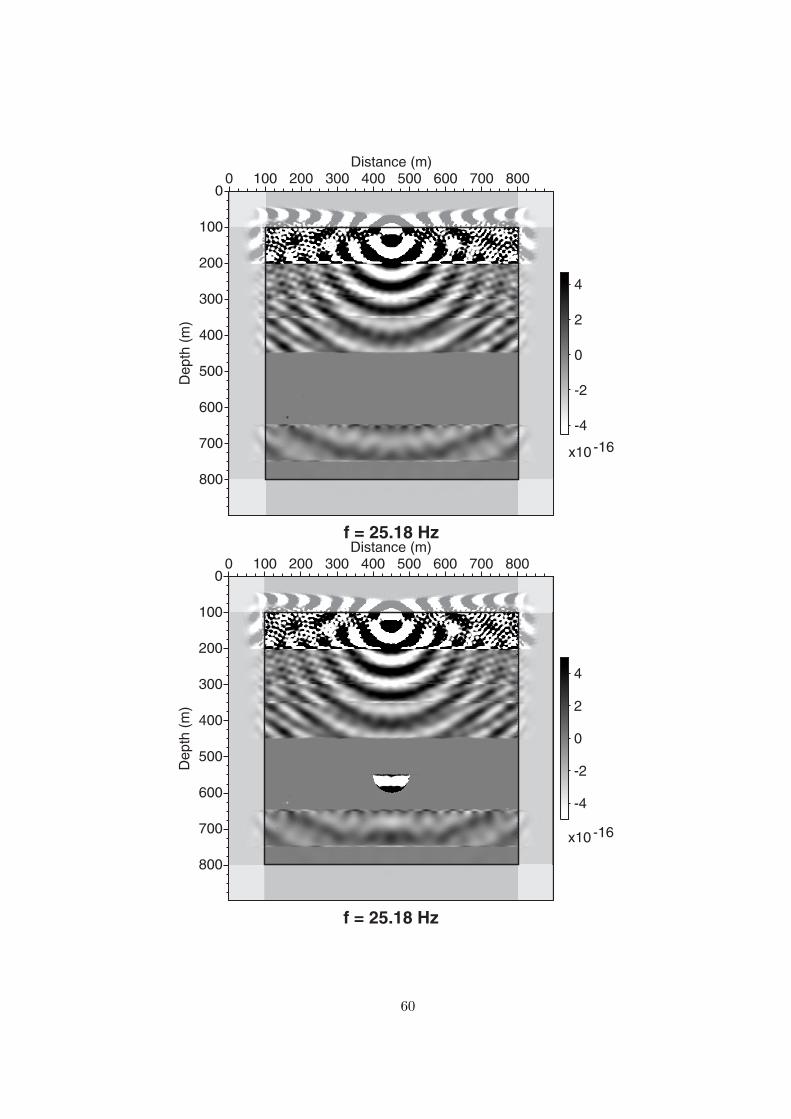
Figure 14 shows two snapshots of monochromatic wavefield of the relative fluid/solid vertical

particle velocity wz at 25 Hz for the cases with and without steam injection. Fluid motions

show higher amplitude in the low cut-off frequency layers, in particular within the steam

injection area. Indeed, in layers with a cut-off frequency above 100 kHz (layers 5, 6 and 8

and heated oil area, see Table 4), the relative fluid/solid particle velocity is between 3 and

4 orders of magnitude lower than in the other layers. In both cases, the time seismograms

of the vertical solid particle velocity uz (Figure 15) display waves interacting with the oil

saturated zone. Despite the complexity of the signal, after the direct transmitted P-wave

arrival, we see a reflection on the top of the central injected steam area while there is a

25

smaller reflection in the case without injection. These reflected and converted waves on the

top of the steam injection zone are underlined on the differential seismogram between the

numerical modellings with and without injection (bottom panel of Figure 15, displayed with

an amplification factor of 2 compared to the top seismograms). The differential seismogram

is hence the seismic response associated to the fluid substitution. Through this complex

example, we illustrate the ability of our approach for accurate modelling which could become

efficient when considering multi-sources problem as for seismic imaging.

CONCLUSION

We have proposed a new numerical method to simulate wave propagation in 2D hetero-

geneous porous media. The homogenisation of porous media leads to consider frequency

dependent parameters and waves regimes (as the flow resistance term and the Biot slow

wave) to take into account diffusive phenomena linked to Biot poroelastodynamics theory.

Thus, we have choosen the DGM, in the space-frequency domain, in order to compute wave

propagation in the whole frequency band without approximation. The DG formulation

builds the fluxes of the eight poroelastodynamic fields between mesh elements. These cells

are triangular and allow us to build complex interfaces and topographies and to adapt locally

cell sizes and interpolation orders (hp-adaptivity). The P1 and P2 orders have been imple-

mented but full simulations with these high orders are still quite expensive numerically and,

consequently, we expect to use these P1 and P2 orders locally to enhance solution precision

around interfaces or sources. The spreaded (P0 order) and punctual (P1 and P2 orders)

sources are validated with respect to the diffusive Biot wave. PML absorbing conditions

are implemented quite naturally in the frequency domain at the edges of the propagation

medium. A good agreement with reflectivity simulations in stratified media is shown for

26

the entire frequency band and so for various Biot wave regimes. An example of a laterally

variable medium is given as an illustration of the poroelastic waves modelling in 2D het-

erogeneous medium. More complex descriptions of the porous medium (double porosity,

patchy saturation...) can be implemented by homogenisation in order to study waveform

attenuations as we may foresee for future works. Morevover, a sensibility study of porous

parameters can be carried out to compute sensitivity kernels. These sensitivity kernels can

then be used to perform time differential imaging by full waveform inversion techniques: a

difficult challenge in subsurface surveys such as for landslides, geotechnical and reservoir

issues in order to better estimate porosity, permeability and fluid properties time variations.

ACKNOWLEDGEMENTS

The project is supported by the ANR ”Captage et Stockage de CO2” program (ANR-

07-PCO2-002) and by national computer centers IDRIS and CINES through the project

046091. Louis De Barros is funded by the department of Communications, Energy and

Natural Ressources (Ireland) under the National Geosciences program. The LU factoriza-

tion of the impedance matrix was performed with MUMPS available on http://graal.ens-

lyon.fr/MUMPS/index.html. The mesh generation was performed with help of TRIANGLE,

available on http://www.cs.cmu.edu/quake/triangle.html. We thank C. Morency, J. D. De

Basabe and an anonymous reviewer for the pertinent and helpful review of this paper.

27

APPENDIX A

PROJECTION MATRICES

Projection matrices are needed for the estimation of fluxes in equation 16.

28

N1x =

1 1 0 0

0 0 1 0

0 0 0 0

0 0 0 0

N2

x =

0 0 0 1

0 0 0 0

0 0 0 0

0 0 0 0

N3

x =

0 0 0 0

0 0 0 0

1 1 0 0

0 0 1 0

N4x =

0 0 0 0

0 0 0 0

0 0 0 1

0 0 0 0

N1

z =

0 0 1 0

1 −1 0 0

0 0 0 0

0 0 0 0

N2

z =

0 0 0 0

0 0 0 1

0 0 0 0

0 0 0 0

N3z =

0 0 0 0

0 0 0 0

0 0 1 0

1 −1 0 0

N4

z =

0 0 0 0

0 0 0 0

0 0 0 0

0 0 0 1

M1

x =

1 0 0 0

0 0 0 0

0 0 0 0

0 0 0 0

M2x =

0 0 1 0

0 0 0 0

0 0 0 0

0 0 0 0

M3

x =

0 0 0 0

1 0 0 0

0 1 0 0

0 0 0 0

M4

x =

0 0 0 0

0 0 0 0

0 0 0 0

1 0 0 0

M5x =

0 0 0 0

0 0 0 0

0 0 0 0

0 0 1 0

M1

z =

0 1 0 0

0 0 0 0

0 0 0 0

0 0 0 0

M2

z =

0 0 0 1

0 0 0 0

0 0 0 0

0 0 0 0

M3z =

0 0 0 0

0 −1 0 0

1 0 0 0

0 0 0 0

M4

z =

0 0 0 0

0 0 0 0

0 0 0 0

0 1 0 0

M5

z =

0 0 0 0

0 0 0 0

0 0 0 0

0 0 0 1

29

REFERENCES

Amestoy, P. R., Duff, I. S., and L’Excellent, J. Y. (2000). Multifrontal parallel distributed

symmetric and unsymmetric solvers. Computer Methods in Applied Mechanics and En-

gineering, 184:501–520.

Amestoy, P. R., Guermouche, A., L’Excellent, J. Y., and Pralet, S. (2006). Hybrid schedul-

ing for the parallel solution of linear systems. Parallel Computing, 32:136–156.

Auriault, J.-L., Borne, L., and Chambon, R. (1985). Dynamics of porous saturated media,

checking of the generalized law of Darcy. Journal of Acoustical Society of America,

77(5):1641–1650.

Berenger, J.-P. (1994). A perfectly matched layer for absorption of electromagnetic waves.

Journal of Computational Physics, 114:185–200.

Biot, M. (1956). Theory of propagation of elastic waves in a fluid-saturated porous solid. I.

low-frequency range, II. higher frequency range. Journal of Acoustical Society of America,

28:168–191.

Bouchon, M. (1981). A simple method to calculate Green’s functions for elastic layered

media. Bulletin of the Seismological Society of America, 71(4):959–971.

Boutin, C., Bonnet, G., and Bard, P. (1987). Green functions and associated source in

infinite and stratified poroelastic media. Geophysical Journal of the Royal Astronomical

Society, 90:521–550.

Brossier, R. (2010). Two-dimensional frequency-domain visco-elastic full-waveform inver-

sion: parallel algorithms, optimization and performances. Computers and Geosciences,

doi:10.1016/j.cageo.2010.09.013

30

Brossier, R., Etienne, V., Operto, S., and Virieux, J. (2010). Frequency-domain numerical

modelling of visco-acoustic waves based on finite-difference and finite-element discontin-

uous galerkin methods. In Dissanayake, D. W., editor, Acoustic Waves, pages 125–158.

SCIYO.

Brossier, R., Operto, S., and Virieux, J. (2009). Seismic imaging of complex onshore struc-

tures by 2D elastic frequency-domain full-waveform inversion. Geophysics, 74(6):WCC63–

WCC76.

Brossier, R., Virieux, J., and Operto, S. (2008a). 2D frequency-domain elastic full-waveform

inversion using a P0 finite volume forward problem. In Expanded Abstracts, 78th Annual

SEG Conference & Exhibition, Las Vegas. Society of Exploration Geophysics.

Brossier, R., Virieux, J., and Operto, S. (2008b). Parsimonious finite-volume frequency-

domain method for 2-D P-SV-wave modelling. Geophysical Journal International,

175(2):541–559.

Brown, R. (1980). Connection between formation factor for electrical resistivity and

fluid-solid coupling factor for Biot’s equation in fluid filled porous media. Geophysics,

45(8):1269–1275.

Burridge, R. and Vargas, C. (1979). The fundamental solution in dynamic poroelasticity.

Geophysical Journal of the Royal Astronomical Society, 58:61–90.

Carcione, J. (1996). Wave propagation in anisotropic, saturated porous media: Plane-wave

theory and numerical simulation. Journal of Acoustical Society of America, 99(5):2655–

2666.

31

Carcione, J., Morency, C., and Santos, J. (2010). Computational poroelasticity - a review.

Geophysics, 75(5):229–243.

Carcione, J. M. and Goode, G. Q. (1995). Some aspects of the physics and numerical

modeling of Biot compressional waves. Journal of Computational Acoustics, 154:261–

272.

Dai, N., Vafidis, A., and Kanasewich, E. (1995). Wave propagation in heteregeneous porous

media: A velocity-stress, finite-difference method. Geophysics, 60(2):327–340.

De Barros, L. and Dietrich, M. (2008). Perturbations of the seismic reflectivity of a fluid-

saturated depth-dependent poroelastic medium. Journal of Acoustical Society of America,

123(3):1409–1420.

De Barros, L., Dietrich, M., and Valette, B. (2010). Full waveform inversion of seismic waves

reflected in a stratified porous medium. Geophysical Journal International, 182(3):1543–

1556.

De la Puente, J., Dumbser, M., Kaser, M., and Igel, H. (2008). Discontinuous Galerkin

methods for wave propagation in poroelastic media. Geophysics, 73(5):77–97.

Drossaert, F. H. and Giannopoulos, A. (2007). A nonsplit complex frequency-shifted PML

based on recursive integration for FDTD modeling of elastic waves. Geophysics, 72(2):T9–

T17.

Dutta, A. J. and Ode, H. (1979). Attenuation and dispersion of compressional waves in

fluid-filled porous rocks wih partial gas saturation. Geophysics, 44(11):1777–1788.

Etienne, V., Virieux, J., and Operto, S. (2009). A massively parallel time domain discontin-

32

uous Galerkin method for 3D elastic wave modeling. In Expanded Abstracts, 79th Annual

SEG Conference & Exhibition, Houston. Society of Exploration Geophysics.

Garambois, S. and Dietrich, M. (2002). Full waveform numerical simulations of seismo-

electromagnetic wave conversions in fluid-saturated stratified porous media. Journal of

Geophysical Research, 107:10.1029/2001JB000316.

Gassmann, F. (1951). Uber die elastizitat poroser medien. Vierteljahrsschrift der Natur-

forschenden Gesellschaft in Zurich, 96:1–23.

Haartsen, M. and Pride, S. (1997). Electroseismic waves from point sources in layered

media. Journal of Geophysical Research, 102(B11):745–769.

Hesthaven, J. S. and Warburton, T. (2008). Nodal Discontinuous Galerkin Method. Algo-

rithms, Analysis, and Application. Springer, New York.

Hustedt, B., Operto, S., and Virieux, J. (2004). Mixed-grid and staggered-grid finite dif-

ference methods for frequency domain acoustic wave modelling. Geophysical Journal

International, 157:1269–1296.

Johnson, D., Koplik, J., and Dashen, R. (1987). Theory of dynamic permeability and

tortuosity in fluid-saturated porous media. Journal of Fluid Mechanics., 176:379–402.

Kennett, B. and Kerry, N. (1979). Seismic waves in a stratified half space. Geophysical

Journal of the Royal Astronomical Society, 57:557–583.

Martin, R., Komatitsch, D., and Ezziani, A. (2008). An unsplit convolutional perfectly

matched layer improved at grazing incidence for seismic wave propagation in poroelastic

media. Geophysics, 73(4):51–61.

33

Masson, Y. and Pride, S. (2010). Finite-difference modeling of Biot’s poroelastic equations

across all frequencies. Geophysics, 75(2):33–41.

Morency, C., Luo, Y., and Tromp, J. (2009). Finite-frequency kernels for wave propaga-

tion in porous media based upon adjoint methods. Geophysical Journal International,

179:1148–1168.

Morency, C. and Tromp, J. (2008). Spectral-element simulations of wave propagation in

porous media. Geophysical Journal International, 175:301–345.

Plessix, R.-E. (2006). A review of the adjoint-state method for computing the gradient of a

functional with geophysical applications. Geophysical Journal International, 167(2):495–

503.

Plessix, R. E. (2007). A Helmholtz iterative solver for 3D seismic-imaging problems. Geo-

physics, 72(5):SM185–SM194.

Plona, T. (1980). Observation of a second bulk compressional wave in a porous medium at

ultrasonic frequencies. Applied Physics Letters, 36(4):259–261.

Pratt, R. G., Shin, C., and Hicks, G. J. (1998). Gauss-Newton and full Newton methods in

frequency-space seismic waveform inversion. Geophysical Journal International, 133:341–

362.

Pride, S. (2005). Relationships between seismic and hydrological properties, pages 253–284.

Water Science and Technology Library, Springer, The Netherlands.

Pride, S. and Berryman, J. (2003). Linear dynamics of double-porosity dual-permeability

materials. i. Governing equations and acoustic attenuation. Physical Review E, 68:036603.

34

Pride, S., Gangi, A., and Morgan, F. (1992). Deriving the equations of motion for porous

isotropic media. Journal of Acoustical Society of America, 92(6):3278–3290.

Pride, S. and Garambois, S. (2002). The role of Biot slow waves in electroseismic wave

phenomena. Journal of Acoustical Society of America, 111:697–706.

Pride, S. and Garambois, S. (2005). Electroseismic wave theory of frenkel and more recent

developements. Journal of Engineering Mechanics, pages 898–907.

Remaki, M. (2000). A new finite volume scheme for solving Maxwell’s system. COMPEL,

19(3):913–931.

Shewchuk, J. R. (1996). Triangle: Engineering a 2D Quality Mesh Generator and Delaunay

Triangulator. In Applied Computational Geometry: Towards Geometric Engineering,

volume 1148, pages 203–222.

Stekl, I. and Pratt, R. G. (1998). Accurate viscoelastic modeling by frequency-domain finite

difference using rotated operators. Geophysics, 63:1779–1794.

Stern, M., Bedford, A., and Millwater, M. (2003). Wave reflection from a sediment layer

with depth dependent properties. Journal of Acoustical Society of America, 77:1781–1788.

Wenzlau, F. and Muller, T. (2009). Finite-difference modeling of wave propagation and

diffusion in poroelastic media. Geophysics, 74(4):55–66.

White, J. E. (1975). Computed seismic speeds and attenuation in rocks with partial gas

saturation. Geophysics, 40(2):224–232.

35

TABLES

Ks (GPa) 40

Gs (GPa) 10

ρs (kg/m3) 2700

Kf (GPa) 2.2

ρf (kg/m3) 1000

η (Pa.s) 0.001

m 1

φ 0.4

k0 (m2) 10−11

cs 5

fc (Hz) 6400

Biot wave regime Diffusive

VP (m/s) 2570

VS (m/s) 860

VBiot (m/s) 160

Table 1: Physical parameters of infinite medium. The P, S and Biot wave velocities (VP ,

VS and VBiot) are given at the central source frequency (200 Hz).

36

Layer 1 Layer 2a Layer 2b Layer 2c

Ks (GPa) 50 40 40 40

Gs (GPa) 30 10 10 10

ρs (kg/m3) 2700 2700 2700 2700

Kf (GPa) 2.2 2.2 2.2 2.2

ρf (kg/m3) 1000 1000 1000 1000

η (Pa.s) 0.001 0.001 0.001 10−7

m 1.5 1 1 1

φ 0.1 0.4 0.4 0.4

k0 (m2) 10−14 10−11 10−9 10−11

cs 5 5 5 5

fc (Hz) 3.2 106 6400 64 0.64

Biot wave regime Diffusive Intermediate Propagative

VP (m/s) 4610 2570 2610 2630

VS (m/s) 2470 860 940 960

VBiot (m/s) 10 160 1170 1340

Table 2: Physical parameters of the two-layer porous medium for the diffusive (layer 2a),

intermediate (layer 2b) and propagative (layer 2c) behaviours of the Biot wave. The P,

S and Biot wave velocities (VP , VS and VBiot) are given at the central source frequency

(200 Hz).

37

Poroelastic Elastic

Order P0 P1 P2 P0 P1 P2

Number of cells 13000 16000 1000 13000 16000 1000

Number of unknowns (∗106) 2.1 19 5.7 0.89 7.2 1.8

Time for matrix building 0.1 s 1.6 s 0.5 s 0.07 s 0.6 s 0.2 s

Time for analysis and factorisation 3.6 s 43 s 23 s 1.4 s 9.4 s 2.3 s

Maximum memory for one processor 130 Mb 1290 Mb 270 Mb 70 Mb 320 Mb 120 Mb

Table 3: Comparison of different numerical parameters for elastic and poroelastic DGM

modelling for P0, P1 and P2 orders. We consider a small (15 m by 15 m) homogeneous

medium and we compute its response on 16 processors (2 nodes of 8 processors).

38

Sand layers Steam Heated

1 2 3 4 5 6 7 8 injection oil

Ks (GPa) 5.2 5.3 5.8 7.5 6.9 37 9.4 26 37 37

Gs (GPa) 2.4 2.9 3.3 4.2 3.6 4.4 5.6 17 4.4 4.4

ρs (kg/m3) 2250 2300 2400 2490 2211 2650 2670 2700 2650 2650

Kf (GPa) 2.5 2.5 2.5 2.5 2.5 1.7 2.5 2.5 0.0014 1.2

ρf (kg/m3) 1040 1040 1040 1040 1040 985 1040 1040 10 900

η (Pa.s) 0.001 0.001 0.001 0.001 0.001 150 0.001 0.001 2.2 10−5 0.3

m 1.5 1.5 1.5 1.5 1.5 1.5 1.5 1.5 1.5 1.5

φ 0.25 0.1 0.05 0.03 0.01 0.33 0.02 0.05 0.33 0.33

k0 (m2) 10−12 10−13 10−13 10−13 10−16 10−12 10−13 10−14 10−12 10−12

cs 20 20 20 20 20 20 20 20 20 20

fc (kHz) 19 48 17 8 1530 4.6 106 4.3 171 66 104

Biot wave regime Diffusive

VP (m/s) 1505 1610 1750 2020 2180 1900 2265 3280 1430 1770

VS (m/s) 330 550 730 940 1120 360 1140 1570 390 360

VBiot (m/s) 15 8 12 17 0.9 0.06 23 6.8 6.9 1.3

Table 4: Physical parameters of the laterally heterogeneous medium (after Dai et al. (1995)).

The P, S and Biot wave velocities (VP , VS and VBiot) are given at the central source frequency

(20 Hz).

39

FIGURE CAPTIONS

40

Figure 1: Variations of parameters with respect to the porosity φ. The top panel shows

density terms related to inertial effects (the fluid density ρf , the mean density ρ and the

flow resistance term ρ are plotted using a dotted line, a continuous line and a dashed

line, respectively). Please note that the flow resistance is clipped as it goes to infinity

for a porosity φ going to zero. The bottom panel shows mechanical terms where elastic

parameter KU is the continuous line, parameter G the dotted line, the coupling parameter

C the dashed line and fluid behaviour parameter M the dotted-dashed line. The clipping

of the parameter M must be underlined as it goes to infinity for a porosity φ going to zero.

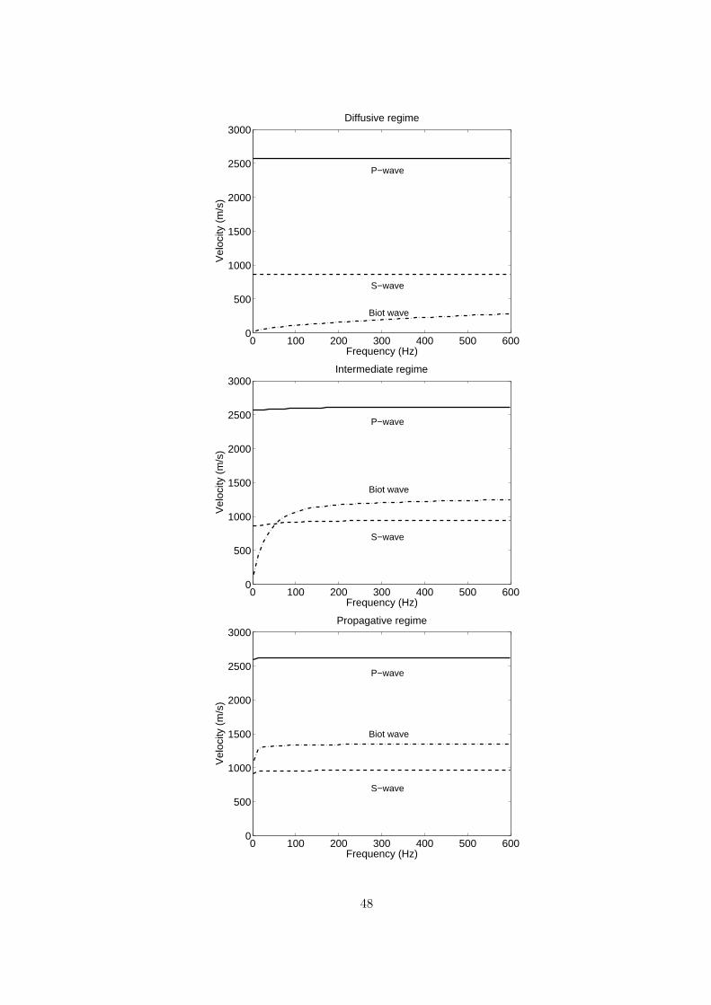
Figure 2: Wave velocities for the three Biot regimes. P (continuous line), S (dashed line)

and Biot (dotted-dashed line) waves velocities as a function of frequency for these three

cases: from the top to the bottom, diffusive regime, intermediate regime and propagative

regime as defined in Table 2. Please note the strong variation of the Biot wave velocity

with respect to the frequency related to the highly dispersive nature of this wave.

Figure 3: Illustration of the meshing for one corner of the numerical model. The PML

structure has parallel lines with respect to the outer edge while a transition zone enables

to move gradually to the inner structured grid based on equilateral triangles, thanks to the

meshing engine we are using: TRIANGLE software by Shewchuk (1996).

41

Figure 4: Frequency maps of the solid vertical particle velocity uz at 110 Hz, 232 Hz,

354 Hz, 476 Hz and 598 Hz (from the top to the bottom). We recall the geometry and

the source position on the top map.

Figure 5: Two time snapshots of solid vertical particle velocity uz at time 0.014 s. The

top snapshot is plotted with the true field amplitude while the bottom one is plotted with

a graphical saturation of 100 in order to detect small parasite numerical reflections coming

from discretized PML zones.

Figure 6: Geometry of the source and the receivers for the infinite medium. Medium

properties are given in Table 1.

Figure 7: Comparison between uz (top panel) and ux (bottom panel) components between

P2 source (continuous) and P0 spreaded source (crosses) for two receivers at x = z = 2 m

and x = z = 5 m. Errors between these solutions are displayed through dashed lines (with

an amplification factor of 10). Medium properties are given in Table 1.

Figure 8: Geometry of the source and the receiver line for the medium composed of two

half-spaces separated by a flat interface. Medium properties are given in Table 2.

42

Figure 9: Flat interface case: seismograms of vertical solid (top panel) and relative

fluid/solid (bottom panel) displacement components (uz and wz) for the diffusive regime.

The SKB solution is in continuous line, DGM in crosses while dashed lines are differences

between the two solutions (multiplied by a factor 5). Medium properties are given in Table

2 (layer 1 and layer 2a). PP and PS2 stand for the converted P and S waves, respectively.

PS1 stands for the conical wave associated to the P direct wave in the first layer. These

two S-waves (PS1 and PS2) are going to be uncoupled at far offset.

Figure 10: Flat interface case: seismograms of vertical solid (top panel) and relative

fluid/solid (bottom panel) displacement components (uz and wz) for the propagative regime.

The SKB solution is in continuous line, DGM in crosses while dashed lines are differences

between the two solutions (multiplied by a factor 5). Medium properties are given in Table

2 (layer 1 and layer 2c). PP, PS2 and PBiot stand for the converted P, S and Biot waves,

respectively. PS1 stands for the conical wave associated to the P direct wave in the first

layer. The two S-waves (PS1 and PS2) are going to be uncoupled at far offset.

43

Figure 11: Flat interface case: seismograms of vertical solid (top panel) and relative

fluid/solid (bottom panel) displacement components (uz and wz) for the intermediate

regime. The SKB solution is in continuous line, DGM in crosses while dashed lines are

differences between the two solutions (multiplied by a factor 5). Medium properties are

given in Table 2 (layer 1 and layer 2b). PP and PS2 stand for the converted P and S waves,

respectively. PS1 stands for the conical wave associated to the P direct wave in the first

layer. These two S-waves (PS1 and PS2) are going to be uncoupled at far offset.

Figure 12: A close-up on seismograms of vertical relative fluid/solid displacement compo-

nent (wz) for the intermediate regime (see Figure 11). The SKB solution is in continuous

line, DGM in crosses while dashed lines are differences between the two solutions. In spite

of the very weak amplitude of the signal, agreement between solutions is still quite good.

Figure 13: Layout of the heterogeneous medium. Medium properties are given in Table 4.

Concentric circles stand for the steam (inner circle) and heated oil extensions (after Dai

et al. (1995)).

Figure 14: Frequency maps of the relative fluid/solid vertical particle velocity wz at a

frequency of 25 Hz for the cases with steam injection (top panel) and without injection

(bottom panel). Please note the injection area with strong amplitudes of motion.

44

Figure 15: Seismograms of vertical solid particle velocity uz for a line of receivers at a depth

of 400 m with respect to the top PML origin for the cases with steam injection (top panel)

and without injection (central panel). The differential seismogram is plotted on the bottom

panel (with an amplification factor of 2). These seismograms show the incident wave as well

as scattering from the injection area after steam substitution and reflections coming from

the deepest interfaces. The seismogram of differences underlines the multiple reflections

and conversions at the top of the injection area.

45

FIGURES

46

0 0.2 0.4 0.6 0.8 1

1000

1500

2000

2500

3000

Porosity

Den

sity

par

amet

ers

(kg/

m3 )

ρ

ρf

ρ

Inertial terms

0 0.2 0.4 0.6 0.8 10

0.5

1

1.5

2

2.5

3

3.5x 10

10

Porosity

Mec

hani

cal p

aram

eter

s (P

a)

KU

G

C

M

Mechanical terms

47

0 100 200 300 400 500 6000

500

1000

1500

2000

2500

3000

Frequency (Hz)

Vel

ocity

(m

/s)

P−wave

S−wave

Biot wave

Diffusive regime

0 100 200 300 400 500 6000

500

1000

1500

2000

2500

3000

Frequency (Hz)

Vel

ocity

(m

/s)

P−wave

S−wave

Biot wave

Intermediate regime

0 100 200 300 400 500 6000

500

1000

1500

2000

2500

3000

Frequency (Hz)

Vel

ocity

(m

/s)

P−wave

S−wave

Biot wave

Propagative regime

48

PML

Transitionarea

Propagationarea

49

0

10

20

30

40

50

60

70

80

De

pth

(m

)

0 10 20 30 40 50 60 70 80Distance (m)

f = 110.80 Hz

-4

-2

0

2

4

x10 -10

Pa

rtic

le v

elo

city V

z

Source

PML

0

10

20

30

40

50

60

70

80

De

pth

(m

)

0 10 20 30 40 50 60 70 80Distance (m)

f = 232.80 Hz

-5

0

5

x10 -10

Pa

rtic

le v

elo

city V

z

0

10

20

30

40

50

60

70

80

Depth

(m

)0 10 20 30 40 50 60 70 80

Distance (m)

f = 354.80 Hz

-4

-2

0

2

4

x10 -10

Part

icle

velo

city V

z0

10

20

30

40

50

60

70

80

Depth

(m

)

0 10 20 30 40 50 60 70 80Distance (m)

f = 476.80 Hz

-5

0

5

x10 -11

Part

icle

velo

city V

z

0

10

20

30

40

50

60

70

80

Depth

(m

)

0 10 20 30 40 50 60 70 80Distance (m)

f = 598.80 Hz

-4

-2

0

2

4

x10 -12

Part

icle

velo

city V

z

50

0

10

20

30

40

50

60

70

De

pth

(m

)0 10 20 30 40 50 60 70

Distance (m)

-5

0

5

x10 -12

Fie

ld in

ten

sity

Source

0

10

20

30

40

50

60

70

Depth

(m

)

0 10 20 30 40 50 60 70Distance (m)

-5

0

5

x10 -14

Fie

ld inte

nsity

Source

51

Source

PML

Receiver 1

6 m

6 m

2 m

Receiver 2

0

1

2

5

Depth(m)

-1 0 1 4Offset (m)

52

0 0.005 0.01 0.015−2

−1

0

1

2

3

4

5

Time (s)

Offs

et (

m)

0 0.005 0.01 0.015−2

−1

0

1

2

3

4

5

Time (s)

Offs

et (

m)

53

Source

PML

Receivers

40 m

40 m

5 m

5 m

37 m

Interface

54

0.01 0.02 0.03 0.04 0.05 0.065

10

15

20

25

30

35

40

Time (s)

Offs

et (

m)

PP PS1 PS2

0.01 0.02 0.03 0.04 0.05 0.065

10

15

20

25

30

35

40

Time (s)

Offs

et (

m)

PP PS1 PS2

55

0.01 0.02 0.03 0.04 0.05 0.065

10

15

20

25

30

35

40

Time (s)

Offs

et (

m)

PP PBiot PS1 PS2

0.01 0.02 0.03 0.04 0.05 0.065

10

15

20

25

30

35

40

Time (s)

Offs

et (

m)

PP PBiot PS1 PS2

56

0.01 0.02 0.03 0.04 0.05 0.065

10

15

20

25

30

35

40

Time (s)

Offs

et (

m)

PP PS1 PS2

0.01 0.02 0.03 0.04 0.05 0.065

10

15

20

25

30

35

40

Time (s)

Offs

et (

m)

PP PS1 PS2

57

0.028 0.03 0.032 0.034 0.036 0.0385

6

7

8

9

10

11

12

Time (s)

Offs

et (

m)

58

700 m

900

75 m50 m

Layer 1

Layer 2

Layer 3

Layer 4

Layer 5

Layer 7

Layer 8

Layer 6

PML

Source

Steam injection

Receivers

Heated oil

100

200

300

350

450

550

650

750

800

0

Depth (m)

59

60

61