wave turbulence and intermittencymath.arizona.edu/~anewell/publications/wave... · wave turbulence...

Physica D 152–153 (2001) 520–550

Wave turbulence and intermittency

Alan C. Newell∗,1, Sergey Nazarenko, Laura BivenDepartment of Mathematics, University of Warwick, Coventry CV4 71L, UK

Abstract

In the early 1960s, it was established that the stochastic initial value problem for weakly coupled wave systems has a naturalasymptotic closure induced by the dispersive properties of the waves and the large separation of linear and nonlinear time scales.One is thereby led to kinetic equations for the redistribution of spectral densities via three- and four-wave resonances togetherwith a nonlinear renormalization of the frequency. The kinetic equations have equilibrium solutions which are much richer thanthe familiar thermodynamic, Fermi–Dirac or Bose–Einstein spectra and admit in addition finite flux (Kolmogorov–Zakharov)solutions which describe the transfer of conserved densities (e.g. energy) between sources and sinks. There is much one canlearn from the kinetic equations about the behavior of particular systems of interest including insights in connection with thephenomenon of intermittency. What we would like to convince you is that what we call weak or wave turbulence is every bit asrich as the macho turbulence of 3D hydrodynamics at high Reynolds numbers and, moreover, is analytically more tractable. It isan excellent paradigm for the study of many-body Hamiltonian systems which are driven far from equilibrium by the presenceof external forcing and damping. In almost all cases, it contains within its solutions behavior which invalidates the premiseson which the theory is based in some spectral range. We give some new results concerning the dynamic breakdown of theweak turbulence description and discuss the fully nonlinear and intermittent behavior which follows. These results may alsobe important for proving or disproving the global existence of solutions for the underlying partial differential equations. Waveturbulence is a subject to which many have made important contributions. But no contributions have been more fundamentalthan those of Volodja Zakharov whose 60th birthday we celebrate at this meeting. He was the first to appreciate that thekinetic equations admit a far richer class of solutions than the fluxless thermodynamic solutions of equilibrium systems andto realize the central roles that finite flux solutions play in non-equilibrium systems. It is appropriate, therefore, that we callthese Kolmogorov–Zakharov (KZ) spectra. © 2001 Elsevier Science B.V. All rights reserved.

Keywords: Wave turbulence; Intermittency; Asymptotic closure; Cumulants

1. Introduction and motivation

Turbulence is about understanding the long-time statistical properties of solutions of nonlinear field equationswith sources and sinks, and in particular with calculating transport. Sometimes the transport is in physical spacesuch as the flux of heat carried across a layer of fluid by turbulent convection, or the flux of momentum from afast moving turbulent stream to a fixed plate or the flux of angular momentum across an annulus from an innerrotating cylinder to slower moving outer one. However, the transport can also be in Fourier space, such as the fluxof energy from large energy containing scales to small scales where dissipation occurs, and it is the description ofthis transport that is the main topic of this lecture.

∗ Corresponding author.E-mail address: [email protected] (A.C. Newell).

1 Also at University of Arizona, Tucson, AZ 85721, USA.

0167-2789/01/$ – see front matter © 2001 Elsevier Science B.V. All rights reserved.PII: S0 1 6 7 -2 7 89 (01 )00192 -0

A.C. Newell et al. / Physica D 152–153 (2001) 520–550 521

The picture we have in mind is this. We have a source of energy at large scales, throughput at middle scales(windows of transparency, inertial ranges) over which the system is essentially conservative and Hamiltonian, anddissipative output at small scales. Among other things, we would like to find solutions of the moment equations forthe unforced, undamped system which describe a finite flux of some conserved density, such as energy, across thesewindows of transparency. This picture derives from the Richardson scenario for the complex vorticity and irregularflow fields encountered in 3D, high Reynolds number hydrodynamics, the granddaddy of turbulent systems. Themain role of the energy conserving nonlinear terms (advection and pressure) in the Euler equations is to transferenergy from the large eddies at the integral scale where the system is forced to smaller and smaller eddies andeventually to the viscous sink. If the average kinetic energy E = 〈u2〉 is written as

∫∞0 E(k) dk, the dissipation rate

P = 〈νω2〉 as 2ν∫∞

0 k2E(k) dk, then the von Karman–Howarth equation is

∂E(k, t)

∂t= f (k) + T (k) − 2νk2E(k), (1.1)

where f (k), T (k) and 2νk2E(k) represent forcing, nonlinear transfer and damping, respectively. E(k) is the angleaveraged Fourier transform of the two point velocity correlation function. T (k) is the Fourier transform of third-ordermoments.

Since the nonlinear transfer T (k) conserves energy, we may write it as the k derivative of a flux, −∂P/∂k. Then,in the window of transparency,

∂

∂t

∫ b

a

E dk = Pa − Pb,

which can be zero either because Pa = Pb = 0 or because Pa = Pb = P , a constant. The first possibility describesan isolated system and leads to an equidistribution of energy in the interval (a, b). The second possibility allowsfor an energy flux between source and sink, and leads to what is known as the Kolmogorov or finite flux spectrum(see Fig. 1).

However, there is a fundamental difficulty with the moment (cumulant) hierarchy of which (1.1) is the firstmember. The hierarchy is unclosed and infinite, and no cumulant discard approximations work. Three-dimensional,high Reynolds number hydrodynamics affords the theoretician no useful approximations, no separation of scales,and no footholds for analytical traction. It is too difficult. Simple fluids are easier to drink than they are to understand.

Nevertheless, some progress in understanding turbulent behavior has come as a result of the formidable insightsof Kolmogorov. Arguing that the symmetries of translation and isotropy are restored in the statistical sense and that,in the infinite Reynolds number limit, all small-scale statistical properties depend only on the local scale and theenergy dissipation rate P , one can deduce that

limr→0

limν→0

limt→∞〈(u‖(x + r, t) − u‖(x, t))n〉 = Cn(Pr)n/3, (1.2)

Fig. 1. Forcing, inertial range and damping regions of k space.

522 A.C. Newell et al. / Physica D 152–153 (2001) 520–550

where u‖ = u · r and Cn are universal constants. The limits correspond to long time and the necessity of stayingaway from the sink and source scales, respectively. But, for almost all n, (1.2) is conjecture. From the Navier–Stokesequations, it can only be proved rigorously for n = 3 [37]. Moreover, recent experimental evidence seems to indicatethat the nth-order structure function, n ≥ 4,

Sn(r) = 〈(u(x + r) − u(x))n〉has index less than 1

3 n. If that is the case, the ratio Sn/(S2)n/2, which in the Kolmogorov theory is a pure constant,diverges as r → 0. The divergence of this ratio indicates that large fluctuations are more probable than Kolmogorovtheory would suggest. The present consensus is that fluctuations in the local dissipation rate are responsible forelevating the tails of the probability density function for velocity differences and for what is generally calledintermittent behavior.

In contrast, the turbulence of a sea of weakly coupled, dispersive wavetrains has a natural asymptotic closure.One can:

1. find a closed kinetic equation for the spectral energy density;2. understand the mechanisms (resonance) by which energy and other conserved densities are redistributed through-

out the spectrum;3. obtain stationary solutions of the kinetic equation analogous to both the thermodynamic and Kolmogorov spectra;4. test the validity of the weak turbulence approximation;

Moreover, the results are not simply a useful paradigm but are of direct interest in their own right in a variety ofcontexts from optics to oceans, from sound to semiconductor lasers to the solar wind.

The natural closure occurs because of two factors, the weak coupling, ε, 0 < ε 1 and the dispersive natureof the waves. The combination means that there is an effective separation of time scales. On the linear time scaletL = ω−1

0 , ω0 a typical frequency in the initial spectrum, the higher-order cumulants decay towards a state ofjoint Gaussianity. On the much longer nonlinear time scale tNL = ε−(2r−4)ω−1

0 , nonlinear resonant interactions oforder r, r = 3, 4, 5, bring about coherence and a departure from joint Gaussian behavior. The regeneration of thehigher-order cumulants by nonlinearity occurs in a special way. For example, in the regeneration of the third-ordercumulant (moment), the product of second-order cumulants is more important than the fourth-order cumulant. Thispattern continues. The regeneration of cumulants of order N is dominated by products of lower-order ones. Thisfeature leads to the natural closure.

The new message of this paper is to suggest that wave turbulence is an even richer paradigm for non-equilibriumsystems than previously believed. The reason is simple and dramatic. As the system relaxes to its asymptoticstationary state, the closure equations almost always become non-uniform at some scale we call kNL. If kNL liesnear the ultraviolet (infrared) end of the spectrum, then for all k, k > kNL(k < kNL), the dynamics becomeincreasingly dominated by large fluctuation local events which are intermittent and fully nonlinear. Some areshock-like; others are spawned by condensate formation. We give explicit formulae for kNL in terms of propertiesof the linear dispersion relation, the nonlinear coupling coefficients and the KZ fluxes.

2. Wave turbulence: asymptotic closure

The derivation of the closed equations for the long-time behavior of the statistical moments (cumulants) and adiscussion of their properties is carried out in a series of seven steps.

1. The set up: the equation for the Fourier amplitudes.2. Moments, cumulants.


3. The cumulant (BBGKY) hierarchy.4. The strategy for solution and the dynamics.5. Resonant manifolds and asymptotic expansions.6. The closure equations.7. Properties: conservation laws, reversibility, finite flux solutions and their temporal formation.

2.1. The set up: equation for Fourier amplitudes

Consider a system which in the linear limit admits wavetrain solutions us = exp(ik · x + iωs(k)t), where ωs(k)

is the dispersion relation and s labels the degree of degeneracy which corresponds to the order of the system orthe number of frequencies corresponding to a given wavevector k. Often, s = +, − corresponding to second-ordersystems where waves travel in one of two directions. By an appropriate choice of canonical variables (sometimessuggested by the Hamiltonian structure), we write

us(x, t) =∫

As(k, t) eik·x dk, As(k, t) = Ask, As(k, t) = 1

(2π)d

∫us(x, t) e−ik·x dx, (2.1)

and find (for ωs = sω(k), s = +, −, ω(k) = ωk),

dAsk

dt− isωkAs

k = ε∑s1s2

∫L

ss1s2kk1k2

As1k1

As2k2

δ(k1 + k2 − k) dk12

+ε2∑

s1s2s3

∫L

ss1s2s3kk1k2k3

As1k1

As2k2

As3k3

δ(k1 + k2 + k3 − k) dk123 + · · · . (2.2)

Remark.

1. Since the class of functions we are dealing with are bounded and non-decaying as |x| → ∞, Ask is not an

ordinary function but a generalized one. However, as we shall see, for spatially homogeneous systems, ensembleaverages of products of the Fourier amplitudes have good properties.

2. Notation: δ12,0 = δ(k1 + k2 − k), dk12 = dk1 dk2, etc.3. ε, 0 < ε 1, is a measure of nonlinearity.

The system Hamiltonian takes the form

H = 1

2

∑s

∫ωkAs

kA−s−k dk + · · · . (2.3)

Examples.Example (a).

1. Optical waves of diffraction in nonlinear media [32,40,45].2. Superfluids [32,53].

These examples are described by the nonlinear Schrödinger equation for a complex field u(x, t), x ∈ Rd, t ∈ R.

∂u

∂t+ i∇2u + iau2u∗ = 0 a constant,

∂u

∂t= i

δH

δu∗ , H =∫ (

∇u · ∇u∗ − a

2u2u∗2

)dx,

u(x, t) = u+ =∫

A+k eik·x dk, u∗(x, t) = u− =

∫A−

k eik·x dk, A−k = A+∗

−k. (2.4)


For fluctuations about the zero state, us = 0,

∂Ask

∂t− isk2As

k = −ias∫

A−sk1

Ask2

Ask3

δ123,0 dk123.

Thus, εLss1s2kk1k2

= 0, ε2Lss1s2s3kk1k2k3

= − 13 iasP123δs1,−sδs2,sδs3,s , ωk = k2.

In Fourier coordinates (Ak = A+k , A∗

k = A−−k)

H =∫

k2A∗kAk dk − a

2

∫A∗

kA∗k1

Ak2Ak3δ01,23 dk0123.

For fluctuations about the condensate state

u = ρ1/20 e−iaρ0t ,

we rewrite (2.4) in polar coordinates

u = ρ1/2 e−iϕ,

and obtain

∂ρ

∂t+ 2∇ · (ρ∇ϕ) = 0,

∂ϕ

∂t+ |∇ϕ|2 + (−a)ρ − 1√

ρ∇2(

√ρ) = 0, (2.5)

which are the Euler equations for a compressible fluid with velocity field 2∇ϕ and pressure p = −aρ2 plus theaddition of the extra term (1/

√p)∇2(

√ρ) sometimes called the quantum pressure. Clearly, ∂p/∂ρ > 0 only when

a < 0. Take a = −1. The Hamiltonian is

H =∫ (

(∇ρ1/2)2 + ρ(∇ϕ)2 + 1

2ρ2)

dx,

and (2.5) is ∂ρ/∂t = δH/δϕ, δϕ/∂t = −δH/δρ. Setting ρ = ρ0 + δρ, ϕ = −ρ0t + δϕ, one finds to quadraticorder that

∂

∂tδρ + k2

0∇2δϕ = −2∇(δρ∇δϕ),∂

∂tδϕ +

(1 − 1

k20

∇2

)δρ = − 1

k40

δρ∇2δρ − 1

2k40

∇2(δρ)2 − (∇(δϕ))2,

where k20 = 2ρ0.

Let

δρ =∫

ρk eik·x dk, δϕ =∫

ϕk eik·x dk, ρk =(

k20k2

2ωk

)1/2∑s

Ask,

ϕk = i

2

(2ωk

k20k2

)1/2∑s

sAsk, ω2

k = k20k2 + k4,

and find

dAsk

dt− isωkAs

k = ε∑s1s2

∫L

ss1s2kk1k2

As1k1

As2k2

δ12,0 dk12 + cubic terms, (2.6)


where

εLss1s2kk1k2

= i√

2

4k0

s1k · k1

(ωω1k2

2

ω2k2k21

)1/2

+ s2k · k2

(ωω2k2

1

ω1k2k22

)1/2

+ss1s2k1 · k2

(ω1ω2k2

ωk21k2

2

)1/2

+(

k2k21k2

2

ωω1ω2

)1/2

s(k1 · k2 − k2)

.

Note: εL+++kk1,k2

= i√

2Vkk1k2 in Ref. [32]. For k0 k, L ∼ L because leading terms cancel. For k0 k, L ∼ k3/2.

In general, for the class of zero mean conservative systems (2.2) for which Ask and A−s

−k are conjugate variablesand As

kt = isδH/δA−s−k , the following properties hold:

1. Lss1···sr

kk1···kr= −L

∗ss1···sr

kk1···kr= −L

−s−s1···−sr

−k−k1···−kr.

2. Lss1···sr

kk1···kris symmetric in (1, 2, . . . , r).

3. Lss1···sr

0k1···kr= 0, k1 + · · · + kr = 0 (except for NLS).

4. Ls1s−s2···−sr

k1k−k2···−kr= (s1/s)L

ss1s2···sr

kk1k2···krwhen k1 + · · · + kr = k.

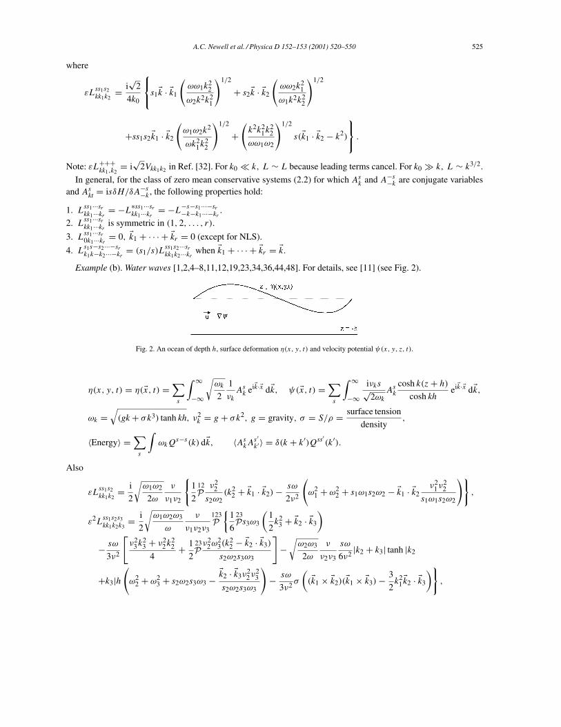
Example (b). Water waves [1,2,4–8,11,12,19,23,34,36,44,48]. For details, see [11] (see Fig. 2).

Fig. 2. An ocean of depth h, surface deformation η(x, y, t) and velocity potential ψ(x, y, z, t).

η(x, y, t) = η(x, t) =∑

s

∫ ∞

−∞

√ωk

2

1

νk

Ask eik·x dk, ψ(x, t) =

∑s

∫ ∞

−∞iνks√2ωk

Ask

cosh k(z + h)

cosh kheik·x dk,

ωk =√

(gk + σk3) tanh kh, ν2k = g + σk2, g = gravity, σ = S/ρ = surface tension

density,

〈Energy〉 =∑

s

∫ωkQs−s(k) dk, 〈As

kAs′k′ 〉 = δ(k + k′)Qss′(k′).

Also

εLss1s2kk1k2

= i

2

√ω1ω2

2ω

ν

ν1ν2

1

2

12P

ν22

s2ω2(k2

2 + k1 · k2) − sω

2ν2

(ω2

1 + ω22 + s1ω1s2ω2 − k1 · k2

ν21ν2

2

s1ω1s2ω2

),

ε2Lss1s2s3kk1k2k3

= i

2

√ω1ω2ω3

ω

ν

ν1ν2ν3

123P

1

6

23Ps3ω3

(1

2k2

3 + k2 · k3

)

− sω

3ν2

[ν2

3k23 + ν2

2k22

4+ 1

2

23P

ν22ω2

3(k22 − k2 · k3)

s2ω2s3ω3

]−√

ω2ω3

2ω

ν

ν2ν3

sω

6ν2|k2 + k3| tanh |k2

+k3|h(

ω22 + ω2

3 + s2ω2s3ω3 −k2 · k3ν2

2ν23

s2ω2s3ω3

)− sω

3ν2σ

((k1 × k2)(k1 × k3) − 3

2k2

1k2 · k3

),


where P23 is permutation over (2, 3), P123 over (1, 2, 3). For g σk2, Lss1s2s3kk1k2k3

is homogeneous of order 3, i.e.

Lεk = ε3Lk . For g σk2, Lss1s2kk1k2

is homogeneous of order 94 .

Example (c). Sound waves [13,14,22,38].

p = p0

(ρ

ρ0

)µ

, c2 = µp0

ρ0, ρ = ρ0

(1 +

∑s

∫As

k eik·x dk)

,

vj =∑

s

∫−c2kj

sωk

Ask eik·x dk, ωk = ck,

where p, ρ and vj are pressure, density and the j th component of velocity, respectively.

εLss1s2kk1k2

= ic2

4

(k · k1

s1ω1+

k · k2

s2ω2+ sω

s1ω1s2ω2

k1 · k2

)+ i

4(µ − 2)sω, ε2L

ss1s2s3kk1k2k3

= iωk

12(µ − 2)(µ − 3).

Each is homogeneous in k of degree 1.For examples of weak turbulence in semiconductor lasers, magnetohydrodynamics, coupled oscillators, plasmas

and atmospheric waves, quantum systems see [3,9,10,15–18,20,21,24,28,30,31,39,40,45,46,49].

2.2. Moments, cumulants

But Eq. (2.2) for the Fourier amplitude is only a means to an end. We really want to describe the behavior ofmoments

Mss′···s(N−1)

N (x; r, r ′r ′′, . . . , r(N−2); t) = 〈us(x)us′(x + r) · · · us(N−1)

(x + r(N−2))〉 (2.7)

as time t becomes large.At this stage 〈〉 denotes an ensemble average connected with a joint probability density function (jpdf)

P (us0, us′

1 , . . . , us(N−1)

(N−1)). Namely, P (us0, . . .) dus

0 · · · is the probability that the field us at x lies between us0 and

us0 + dus

0, the field us′at x + r lies between us′

1 and us′1 + dus′

1 , and so on. However, we now make the assumptionof spatial homogeneity. MN only depends on the relative geometry of the configuration and does not depend on thebase coordinate x. In this situation, it is convenient to think of 〈〉 as an average over the base coordinate.

But one should be cautious with the assumption of spatial homogeneity. It is a property of the equations that if MN

is independent of the base point x initially, it will remain so. But suppose MN depends weakly on x initially. Then,the nonlinear dynamics can lead to a steepening of derivatives (cf. Burgers equation) and a possible breakdown ofspatial homogeneity into patches separated by shocks. In this essay, we ignore this possibility.

Moments are inconvenient for several reasons. In particular MN does not tend to zero as the separations r, r ′, . . .

tend independently to infinity. This means that it does not possess an ordinary Fourier transform which is thecoordinate most relevant when dealing with a field of wavetrains. Therefore, we use cumulants which are related ina 1:1 fashion with the moments.

Ms1(t) = 〈us(x)〉 = R(1)s(t) = us(x),

Mss′2 (r, t) = 〈us(x)us′

(x + r)〉 = us(x)us′(x + r) + us(x)us′

(x + r) = R(2)ss′(r) + R(1)sR(1)s′,

Mss′s′′3 (r, r ′, t) = 〈us(x)us′

(x + r)us′′(x + r ′′)〉 = R(3)ss′s′′

(r, r ′) + one of all possible partitions,

M(N)ss′···N = R(N)ss′··· + one of all possible partitions.


Curly brackets denote cumulants, and angle brackets are moments. We will also study systems where M1 = 〈u〉 ≡ 0.Then,

Mss′2 (r) = R(2)ss′(r) = 〈us(x)us′

(x + r)〉,Mss′s′′

3 (r, r ′) = R(3)ss′s′′(r, r ′) = 〈us(x)us′

(x + r)us′′(x + r ′)〉,

Mss′s′′s′′′4 (r, r ′, r ′′) = R(4)ss′s′′s′′′

(r, r ′, r ′′) + R(2)ss′(r)R(2)s′′s′′′(r ′′ − r ′) + R(2)ss′′(r ′)R(2)s′s′′

(r ′′ − r)

+R(2)ss′′′(r ′′′)R(2)s′s′′(r ′ − r), · · · .

R(N)ss′···s(N−1)(r, r ′, . . . , r(N−2)) have the property that R(N) → 0 as |r|, |r ′|, . . . tend to infinity independently and

in any directions because it is reasonable to assume, at least at one particular time when the fields are first stirred,that the statistics of widely separated points are uncorrelated.

This means that its Fourier transforms Q(N),

R(N)ss′···s(N−1)

(r, r ′, . . . , r(N−2)) =∫

Q(N)ss′···s(N−1)

(k′, k′′, . . . , k(N−1)) eik′·r+ik′′·r ′+···+ik(N−1)·r(N−2)

dk′

× dk′′ · · · dk(N−1),

Q(N)ss′···s(N−1)

(k′, k′′, . . . , k(N−1)) = 1

(2π)(N−1)d

∫R(N)ss′···s(N−1)

(r, r ′, . . . , r(N−2)) e−ik′·r···−ik(N−1)·r(N−2)

× dr dr ′ · · · dr(N−2) (2.8)

are smooth functions, at least at one time.

Remark.

1. The dynamics will produce non-smooth components due to nonlinearities. Indeed, understanding these non-smooth behaviors is the key to understanding the long-time behavior of wave turbulent fields.

2. The notation of pairing k′ with r, k′′ with r ′, . . . and k(N−1) with r(N−2) is a matter of future convenience.

2.3. The cumulant hierarchy

We now introduce the dynamics by writing down the equations for the Fourier space cumulants Q(2)ss′(k′),Q(3)ss′s′′

(k′, k′′), . . . , Q(N)ss′···s(N−1)(k′, k′′, . . . , k(N−1)). To do this, we first seek a relationship between averages

of products of the Fourier amplitudes Ask and the Fourier cumulants Q(N).

We know already that

Ask = 1

(2π)d

∫us(x) e−ik·x dx

is not an ordinary function because us(x) does not tend to zero as |x| → ∞. It is simply bounded there.If us(x) were a finite sum of wavetrains, us(x) = ∑

j Asj eikj ·x , then As

k = ∑j As

j δ(k − kj ), namely the sum ofcomplex numbers times Dirac delta functions. Interacting wavetrains transfer energy via three-wave interactions ona time scale of ω0t = O(1/ε). To see this, write As

k in the above form, solve (2.2) iteratively and find that the zerodenominators first enter when one calculates the first iterate at order ε.

If us(x) were to belong to a set of smooth fields which decayed sufficiently rapidly as |x| → ∞, then As(k, t)

would be smooth and the asymptotic expansion As(k, t) = as0(k) eisωkt + εAs

1(k, t) + · · · would remain uniformlyvalid in time. This is because the small denominators appear in integrals in the combination −iW−1

12,0(exp(iW12,0t)−1), W12,0 = s1ω1+s2ω2−sω. Even though W12,0 can be zero, from Section 2.5 we will see that As

1(k, t) is bounded


in time (we exclude the case of multiple zeros). Thus, if the fields are sufficiently small and decay sufficiently fastas |x| → ∞, for all intents and purposes, (2.2) behaves as a linear system. The physical reason is that resonantwavetrains are not long enough to have enough time to interact to produce order 1 exchanges of energy.

The fields of interest to us here are bounded at infinity and consist of collections of infinitely long wavetrains (orwavepackets). Because they are infinite in extent, they have enough time to exchange energy and produce long-timecumulative effects. However, because they are not collections of discrete wavetrains, there is additional phase mixingand, due to these statistical cancellations, the non-uniformities (coherences) produced by nonlinear interactions takelonger to appear and energy is exchanged on the time scale ε−2ω−1

0 .To summarize, L2 functions have wavetrains which do not interact long enough to produce order 1 cumulative

changes. Discrete wavetrains interact very strongly and, via r wave resonances, exchange order 1 amounts of energyon the time scale ω0t = O(ε−r+2). Continuous spectra of infinite wavetrains, corresponding to bounded, spatiallyrandom fields, have additional mixing which slows the rate of order 1 energy exchange via r wave resonances tothe time ω0t = O(ε−2(r−2)).

Let us(x) be a spatially homogeneous random field of zero mean. Then, because Ask is a functional of us(x),

〈Ask〉 = 0,

〈AskAs′

k′ 〉 = 1

(2π)2d

∫〈us(x)us′

(x + r)〉 e−ik·x−ik′(x+r) dx d(x + r)

= 1

(2π)2d

∫R(2)ss′(r) e−ik′·r dr

∫e−i(k+k′)·x dx = δ(k + k′)Q(2)ss′(k′) = δ(k + k′)Q(2)ss′(−k).

Note R(2)ss′(r) = R(2)s′s(−r) because

〈us(x)us′(x + r)〉 = 〈us(x′ − r)us′

(x′)〉 = Rs′s(−r).

Likewise

〈AskAs′

k′As′′k′′ 〉 = δ(k + k′ + k′′)

(2π)2d

∫R(3)ss′s′′

(r, r ′) e−ik′·r−ik′′·r ′dr · dr ′ = δ(k + k′ + k′′)Q(3)ss′s′′

(k′, k′′),

〈AskAs′

k′As′′k′′As′′′

k′′′ 〉 = δ(k + k′ + k′′ + k′′′)Q(4)ss′s′′s′′′(k′, k′′, k′′′)

+δ(k + k′)δ(k′′ + k′′′)Q(2)ss′(k′)Q(2)s′′s′′′(k′′′)

+δ(k + k′′)δ(k′ + k′′′)Q(2)ss′′(k′′)Q(2)s′s′′′(k′′′)

+δ(k + k′′′)δ(k′ + k′′)Q(2)ss′′′(k′′′)Q(2)s′s′′(k′′)

For convenience, we often write

Q(2)ss′(k′) as Q(2)ss′(k, k′), remembering k + k′ = 0 and

Q(3)ss′s′′(k′, k′′) as Q(3)ss′s′′

(k, k′, k′′), remembering k + k′ + k′′ = 0.

This allows one to keep better track of symmetries.

Remark. Note Ask is now not a Dirac delta function as it was when us(x) was a sum of discrete wavetrains. Its

products involve, after averaging, a Dirac delta function times a smooth (at least at some initial time) cumulant.The fact that the cumulants containing products of δ functions in 〈As

kAs′k′As′′

k′′As′′′k′′′ 〉 (namely the products of Q(2)’s)

have more potency than the fourth-order cumulant makes for a natural asymptotic closure. The regeneration ofhigher-order cumulants by the dynamics depends only weakly on even higher ones and strongly on products oflower ones.


We build the cumulant hierarchy by multiplying (2.2) by As′k′ , and (2.2), with s, k replaced by s′, k′, by As

k andadding to find, after averaging

dQ(2)ss′(k′)dt

− i(sω + s′ω′)Q(2)ss′(k′)

= 00′P ε∑s1s2

∫L

ss1s2kk1k2

Q(3)s′s1s2(k1, k2)δ12,0 dk12 + 00′P ε2

∑s1s2s3

∫L

ss1s2s3kk1k2k3

Q(4)s1s2s3s′(k1, k2, k3, k′)δ0,123 dk123

+300′P ε2

∑s1s2s3

Q(2)s3s′(k′)

∫L

ss1s2s3kk1−k1k

Q(2)s1s2(−k1) dk1, k + k′ = 0. (2.9)

In (2.9), we have factored out δ(k + k′) and used the symbol P00′to denote rewriting the following term with s, k

replaced by s′, k′ and adding the two contributions together. Multiplying (2.2) by As′k′As′′

k′′ and applying P00′0′′, we

find to order ε

dQ(3)ss′s′′(k′, k′′)

dt− i(sω + s′ω′ + s′′ω′′)Q(3)ss′s′′

(k′, k′′)

= 00′0′′P ε

∑s1s2

∫L

ss1s2kk1k2

Q(4)s′ss′′s1s2(k′′, k1, k2)δ0,12 dk12

+2ε00′0′′P∑s3s4

Lss3s4k−k′−k′′Q

(2)s3s′(k′)Q(2)s4s′′

(k′′) + o(ε2), (2.10)

where k + k′ + k′′ = 0.Note: It is convenient to relabel s1, s2 as s3, s4 in the second term of the right-hand side of (2.10). In addition, we

have used the properties that L = 0 when k = 0 and is symmetric over the indices 1, 2.We continue to build the hierarchy in this way. The reader should write down the equation for Q(4)ss′s′′s′′′

(k′, k′′, k′′′).Note that the consistency of 〈As

k〉 = 0 requires that Lss1s20k1−k1

= 0.

Proof.

d〈Ask〉

dt− isωk〈As

k〉 = ε∑s1s2

∫L

ss1s2kk1k2

〈As1k1

As2k2

〉δ0,12 dk12 = ε∑s1s2

δ(k)

∫L

ss1s20k1k2

Q(2)s2s1(k1) dk1,

d〈Ask〉

dt= 0 when L

ss1s20k1−k1

= 0.

2.4. The strategy for solutions and the dynamics

We solve the cumulant hierarchy of which (2.9) and (2.10) are the first two members as an asymptotic expansionin powers of ε, namely we assume

Q(N)ss′···s(N−1)

(k′, . . . , k(N−1)) = q(N)ss′···s(N−1)

0 (k′, k′′, . . . , k(N−1), t) exp(i(sω + s′ω′

+ · · · + s(N−1)ω(N−1))t) + εQ(N)1 + ε2Q

(N)2 + · · · + εrQ(N)

r + o(εr ).

(2.11)

This means that the difference between Q(N) and any finite sum, say up to εr , divided by εr , tends to zero as ε → 0.We will insist that (2.11) is a valid asymptotic expansion for all time t . To achieve this, we will have to allow q

(N)0

to vary slowly in time.


Remark.

1. Because of non-smoothness which will appear in Q(3)1 , Q

(4)2 in the long-time limit, it is better to interpret the

statement of asymptotic expansions in physical space. Namely, we order Q(N) where it makes sense and, whereit does not, we order the corresponding R(N).

2. We are seeking asymptotic and not convergent series representations of the solutions to (2.9) and (2.10)!

We recognize that, because of small denominators which will occur on resonant manifolds M defined by

k1 + k2 = k, s1ω(k1) + s2ω(k2) = sω(k), (2.12)

non-uniformities in the asymptotic expansions will arise. For example, we will find

limt→∞

ε2t fixed

Q(2)ss′2 (k′) = tQ

(2)ss′2 (k′) + Q

(2)ss′2 (k′)

will contain terms which grow with t and terms which are bounded. As a result, for times ε2t = O(1), the asymptoticexpansion is not well ordered. We restore the well-ordered asymptotic expansion by recognizing that, because ofthese secular terms, there will be an order 1 transfer in spectral energy (i.e. in Q(2)ss′(k′), s′ = −s) over long times.

This transfer is captured by seeking an asymptotic expansion for the time derivative of q(N)ss′···s(N−1)

0 (k′, . . . ,k(N−1)) as

dq(N)ss′···s(N−1)

0 (k′, . . . , k(N−1))

dt= εF

(N)ss′···s(N−1)

1 (k′, . . . , k(N−1))

+ε2F(N)ss′···s(N−1)

2 (k′, . . . , k(N−1)) + · · · , (2.13)

and choosing F(N)1 , F

(N)2 , . . . so as to remove secular terms in (2.11) and render it a well-ordered asymptotic

expansion uniform in time t . Eq. (2.13) is the equation of asymptotic closure. This is closed because

• N = 2, s′ = −s, F(2)1 = 0, F

(2)2 depends only on q−ss

0 (k) = nk(t). This is the kinetic equation and we write itas

dnk

dt= T2[nk] + T4[nk] + · · · . (2.14)

• N = 2, s′ = s and N > 2, F(N)1 = 0, F

(N)2 = iq(N)ss′···s(N−1)

0 (k′, . . . , k(N−1))(Ωsk + · · · + Ωs(N−1)

k(N−1) ) which issolved by frequency renormalization

sωk → sωk + ε2Ωsk + · · · . (2.15)

We, therefore, achieve a natural asymptotic closure for the cumulant hierarchy.It is natural because it does not assume anything about the initial statistical distributions of the fields. They need

not be joint Gaussian. What happens is that the linear behavior of the system brings the system close to a state ofjoint Gaussianity. Non-joint Gaussianity is regenerated by nonlinear interactions, e.g. dQ(3)/dt depends on Q(4)

and products of Q(2). However, it is the products of the lower-order cumulants that give a cumulative long-timeeffect and therefore only they play a role in the long-time dynamics. Hence, one achieves closure.

It is asymptotic because the closure equations (2.13)–(2.15) are long-time “average” equations. They are solvediteratively. To find the behavior for times ω0t = o(ε−2) one solves the truncated equation (2.14) with T4, T6 ignored.To find the behavior for ω0t = o(ε−4) one solves (2.14) with T6, T8, . . . ignored, and so on.


It is important to make several points.

1. Although T2N [nk], N ≥ 1, is formally of order ε2N in (2.14) and ε2N Ωs2Nk, N ≥ 1, is formally of order ε2N in

(2.15), the terms in the series are still functions of k. It turns out that the ratios T2N+2/T2N , ε2Ωs2N+2k/Ωs

2Nk,formally of order ε2, do not in general remain uniformly bounded as k → 0 or k → ∞ when calculated onsolutions of the truncated equations. This fact is the origin of the breakdown of wave turbulence at small andlarge scales. We return to this in Section 4.

2. The term T2 is the kinetic equation (2.14) contains triad (three-wave) resonances. The term T4 has been calculated[12] and contains four-wave resonances and gradients (with respect to k) of three-wave resonances and principalpart integrals. It is not clear how many of these terms can be reabsorbed into T2 by renormalizing the frequencyin the exponent of the Dirac delta function. Often the successive terms in the series are schematically representedin diagram notation.

3. The imaginary part of the renormalized series (2.15) for sωk has positive imaginary part at o(ε2) if there arethree-wave resonances, at o(ε4) if there are four-wave resonances, and so on. This means that, over long times,and due to resonant interactions, the zeroth-order Fourier space cumulants (which essentially correspond to initialdata), N = 2, s′ = s, N ≥ 3, decay exponentially. Their physical space counterparts decay for two reasons.They decay algebraically in t because of the Riemann–Lebesgue lemma and the presence of fast oscillationsmultiplying the zeroth-order Fourier space cumulants.

These remarks must be revisited in those regions of k space where the weak turbulence closure (2.14) and (2.15)is non-uniform in k = |k|.

2.5. Resonant manifolds and asymptotic expansions

Solve (2.9) and (2.10), . . . iteratively.

ε0 :

Q(2)ss′0 (k′, t) = q

(2)ss′0 (k′, t) ei(sω+s′ω′)t , k + k′ = 0,

Q(3)ss′s′′0 (k′, k′′, t) = q

(3)ss′s′′0 (k′, k′′, t) ei(sω+s′ω′+s′′ω′′)t , k + k′ + k′′ = 0,

...

Q(N)ss′···s(N−1)

0 (k′, k′′, . . . , k(N−1)) = q(N)ss′···s(N−1)

0 (k′ · · · k(N−1), t) ei(sω+···+s(N−1)ω(N−1))t ,

k + · · · + k(N−1) = 0.

Note:

• For N = 2, s′ = −s, the oscillatory dependence disappears because ω(−k) = ω′ = ω. q(2)s−s0 (k′, t) is

proportional to the spectral energy density.• In anticipation of non-uniformities in (2.11), we allow the coefficients q

(N)0 vary slowly in time via (2.13).

ε : Q(2)ss′1 (k′, t) = 00′

P∑s1s2

∫L

ss1s2kk1,k2

q(3)s′s1s20 (k1, k2)∆(W12,0) ei(sω+s′ω′)t δ0,12 dk12,

where ∆(x) = (eixt − 1)/ix, W12,0 = s1ω1 + s2ω2 − sω. We need to consider long-time behavior of integrals ofthe form∫

F (k1)eih(k1;k)t − 1

ih(k1; k)dk1,


where h(k1; k) = s1ω(k1) + s2ω(k − k1) − sω(k). The integrals are dominated by values of k1 near a zero ofh(k1; k), the resonant manifold M defined by (2.12),

k1 + k2 = k, s1ω(k1) + s2ω(k2) = sω(k) for some s1, s2, s.

In the neighborhood of

M : h(k1; k) = 0,

we coordinatize k1 (say k1x, k1y if k1 is 2D in a basis locally parallel and perpendicular to M . Let k(0)1 ∈ M . Then

h(k1; k) = h(k(0)1 ; k) + (k1 − k(0)

1 ) · ∇k1h(k(0)

1 ; k) + · · · .

In what follows, we will assume that on M ,

∇k1h(k(0)

1 ; k) = 0 for k(0)1 ∈ M,

and illustrate by example what happens when ∇k1h = 0. Calling the local perpendicular coordinate by x, the above

integral can be written as∫dy

∫f (y, x)

eixt − 1

ixdx.

Therefore, we study

limt→∞

∫f (x)

eixt − 1

ixdx.

In Q(2)1 , the function f (x) (proportional to q

(3)s′s1s20 (k1, k2)) is slowly varying in time so the limit is taken in the

sense that t → ∞, εr t fixed for some r = 1, 2, . . .. The smoothness of q(3)s′s1s20 (k1, k2) is also important. At the

initial time, we have assumed this. If we are to recalculate beginning at some later time t1 = O(1/ε2), an O(ε)

non-smoothness will have developed in the new “initial” state. We will discuss this and show that for limt−t1→+∞it does not contribute whereas for limt−t1→−∞ it does. This is important in resolving an apparent irreversibility

paradox. A little calculation (which can be done many ways, e.g. let f (x) = f (x)−f (0) e−x2 +f (0) e−x2) reveals

lim|t |→∞

∫f (x)

eixt − 1

ixdx = π sgnt f (0) + iP

∫f (x)

xdx,

where

sgnt =+1, t > 0,

−1, t < 0,

and P denotes the Cauchy principal value. Schematically

lim|t |→∞

∆(x) = π sgnt δ(x) + iP

(1

x

).

Returning to Q(2)ss′1 (k′, t), we see that it is bounded as t → ∞. This is important. A non-zero q

(3)s′s1s20 (k1, k2) at

the initial time (here taken to be t = 0) does not affect the uniformity of (2.11). We can begin with initial conditionsfar from joint Gaussian. This was first pointed out by Benney and Saffman [4].


Next, we calculate

Q(3)ss′s′′1 (k′, k′′) = 00′0′′

P∑s1s2

∫L

ss1s2kk1k2

q(4)s′s′′s1s20 (k′′, k1, k2)∆(W12,0) ei(sω+s′ω′+s′′ω′′)t δ0,12 dk12

+2∑s3s4

Lss3s4k−k′−k′′q

(2)s3s′0 (k′)q(2)s4s′′

0 (k′′)∆(s3ω′ + s4ω′′ − sω) ei(sω+s′ω′+s′′ω′′)t

+2∑s3s4

Ls′s3s4k′−k′′−k

q(2)s3s′′0 (k′′)q(2)s4s

0 (k)∆(s3ω′′ + s4ω − s′ω′) ei(sω+s′ω′+s′′ω′′)t

+2∑s3s4

Ls′′s3s4k′′−k−k′q

(2)s3s0 (k)q

(2)s4s′0 (k′)∆(s3ω + s4ω′ − s′′ω′′) ei(sω+s′ω′+s′′ω′′)t . (2.16)

Note: Because there are no integrals left on some of these terms, and because they contain oscillating factors,their long-time limit cannot be directly taken. We, therefore, return to physical space and examine instead theasymptotic well orderedness of the corresponding physical space cumulant R(3). Schematically, however, we canwrite limt→∞∆(x) = π sgnt δ(x)+iP (1/x). The integral in physical space will generally be the product of boundedand oscillatory factors which tend to zero because of the Riemann–Lebesgue lemma. However, for s3 = −s′, s4 =−s′′ in the first, s3 = −s′′, s4 = −s in the second, and s3 = −s, s4 = −s′ in the third, the exponents coalesce∆(−sω − s′ω′ − s′′ω′′) ei(sω+s′ω′+s′′ω′′)t = ∆(sω + s′ω′ + s′′ω′′) and these terms survive the t → ∞ limit.

In Section 4, we will calculate these surviving terms for each R(N) and examine their asymptotic expansionsfor well orderedness. We will find that, consistent with Remark 1 in Section 2.4, they are not always well ordered.Non-uniformities in the corresponding asymptotic expansions for the structure functions can appear at both smalland large separations. This can lead to intermittent behavior dominated by fully nonlinear solutions of the fieldequations. We will discuss this further in Section 4.

As t → ±∞,

Q(3)ss′s′′1 (k′, k′′) → Q

(3)ss′s′′1 (k′, k′′) = 2

(π sgnt δ(sω + s′ω′ + s′′ω′′) + iP

(1

sω + s′ω′ + s′′ω′′

))

·(00′0′′P Ls−s′−s′′

k−k′−k′′q(2)−s′s′0 (k′)q(2)−s′′s′′

0 (k′′)). (2.17)

In our calculation of Q(2)ss′2 (k′), however, we will find that it is Q

(3)s′s1s21 (k1, k2) e−i(sω+s′ω′)t which appears in the

integrand and it is its long-time limit that we will need.

Remark. We now, at O(ε), have seen the appearance of irreversibility in a reversible system. The limit processeffectively ignores all the fluctuating terms so that information on phase is effectively lost in taking the limit.Solutions of the resulting kinetic equations can be attractors.

Before we complete the calculations by identifying the secular terms which appear at O(ε2) and thereby calculatethe kinetic equation and renormalization factors (i.e. F

(N)2 for N ≥ 2), let us return to the study of (2.15) and

illustrate in Example 2 what happens if ∇h · n = 0 (n unit normal to M).

Example 1 (ω = k2). Take k = (k1, 0); k1 = (k1x, k1y),

M : h = k21 + (k − k1)2 − k2 = 2((k1x − 1

2 k)2 + k21y − 1

4 k2).

The resonant manifold for k is M(k) and it is the set of k1 for which h = 0. It is a circle of radius 12 k centered at the

middle of the vector k. We can coordinatize M as follows: k1x = k cos2(θ/2), k1y = k sin(θ/2) cos(θ/2), ∇h =2(k1x − 1

2 k), 2k1y = k(cos θ, sin θ) is never identically zero (∇h · t = 0, ∇h · n = 0).


Example 2 (Acoustic waves: ω = |k|). Here h = s1|k1|+ s2|k − k1|− s|k| is zero when k1 is collinear with k. Now∇h = 0 for all k1 ∈ M . The integral (2.15) now depends critically on dimension. In 2D,

∫f (x)((eiht −1)/ih) dk1 ∼∫

f (x)((eix2t − 1)/ix2) dx ∼ t1/2. In 3D,∫

f (x, y)(ei(x2+y2)t /i(x2 + y2)) dx dy ∼ ln t (see [13,14,38]).

Remark. The web created by the manifolds M(k), M(k1), M(k2), . . . , where k1 ∈ M(k), k2 ∈ M(k1), . . . ,, hasan interesting geometry [42].

2.6. The closure equations

We now come to the final step in the closure calculation, namely the identification of the first terms in (2.11)which are non-uniform, the choices for F

(N)1 , F

(N)2 and the resulting equations for asymptotic closure.

The equation for Q(2)ss′2 (k′) is

d

dt(Q

(2)ss′2 (k′) e−i(sω+s′ω′)t ) + F

(2)ss′2 (k′)=00′

P∑s1s2

∫L

ss1s2kk1k2

(Q(3)s′s1s21 (k1, k2) e−i(sω+s′ω′)t )δ0,12 dk12. (2.18)

From (2.16) (the appearance of the indices 1, 2 here necessitated the use of the dummy indices 3, 4 in (2.16)),

Q(3)s′s1s21 (k′, k1, k2) e−i(sω+s′ω′)t

= 120′P∑s3s4

∫L

s′s3s4k′k3k4

q(4)s1s2s3s40 (k2, k3, k4)∆(W34,0′) ei(s′ω′+s1ω1+s2ω2)t δ0′,34 dk34 · e−i(sω+s′ω′)t

+2∑s3s4

Ls′s3s4k′−k1−k2

q(2)s3s10 (k1)q

(2)s4s20 (k2)∆(s3ω1 + s4ω2 − s′ω′) ei(s′ω′+s1ω1+s2ω2)t e−i(sω+s′ω′)t

+2∑s3s4

Ls1s3s4k1−k2−k′q

(2)s3s20 (k2)q

(2)s4s′0 (k′)∆(s3ω2 + s4ω′ − s1ω1) ei(s′ω′+s1ω1+s2ω2)t e−i(sω+s′ω′)t

+2∑s3s4

Ls2s3s4k2−k′−k1

q(2)s3s′0 (k′)q(2)s4s1

0 (k1)∆(s3ω′ + s4ω1 − s2ω2) ei(s′ω′+s1ω1+s2ω2)t e−i(sω+s′ω′)t .

Note: δ(k′ − k3 − k4) combined with δ(k1 + k2 + k′) implies δ(k1 + k2 + k3 + k4), the Dirac delta function associatedwith q

(4)s1s2s3s40 (k1, k2, k3, k4) in the first term of the above equation. For the second term, strong response occurs

only when s3 = −s1, s4 = −s2 and s′ = −s. The dominant term is

(∗) 2δs′−sLs′−s1−s2k′−k1−k2

q(2)−s1s10 (k1)q

(2)−s2s20 (k2)

(π sgnt δ(s1ω1 + s2ω2 − sω) + iP

1

s1ω1 + s2ω2 − sω

).

Recall also k′ + k = 0. For the third term, strong response occurs when s3 = −s2, s4 = s (any s, s′); the dominantterm is

(∗) 2Ls1−s2sk1−k2kq

(2)−s2s20 (k2)q

(2)ss′0 (k′)


1

s1ω1 + s2ω3 − sω

).

For the fourth term, strong response occurs when s3 = s, s4 = −s1 (any s, s′); the dominant term is

(∗) 2Ls2−s−s1k2k−k1

q(2)ss′0 (k′)q(2)−ss1

0 (k1)


1

s1ω1 + s2ω2 − sω

).

The only terms in Q(2)2 e−i(sω+s′ω′)t which contribute to t growth arise from F

(2)ss′2 (k′) and the three (∗) terms above.

The terms containing q(4)s1s2s3s40 do not contribute to secular growth. Thus, we do not require any assumption on

the initial statistics other than the smoothness of the initial Fourier space cumulants or, equivalently, the decay ofthe physical space cumulants at large separations. We choose F

(2)2 to kill the secular growth.


For s′ = −s, we find

dqs−s0 (−k)

dt= dq−ss

0 (k)

dt= 4πε2 sgnt

∑s1s2

∫L

ss1s2kk1k2

q(2)−ss0 (k)q

(2)−s1s10 (k1)q

(2)−s2s20 (k2)

×

L−s−s1−s2−k−k1−k2

q(2)−ss0 (k)

+ Ls1s−s2k1k−k2

q(2)−s1s10 (k1)

+ Ls2s−s1k2k−k1

q(2)−s2s20 (k2)

δ(s1ω1+s2ω2−sω)δ(k1 + k2 − k) dk1 dk2.

(2.19)

Remark. The principal value terms cancel on the application of P00′ = P0−0. The Dirac delta terms add.

Eq. (2.19) is the kinetic equation for the redistribution of the spectral density q(2)−ss0 (k) via resonant exchange

between the three waves k1, k2, k lying on the manifold M ,

s1ω(k1) + s2ω(k2) = sω(k), k1 + k2 = k : M (2.20)

for some choices of s1, s2, s.For s′ = −s (thus, s′ = s since s2 = s′2 = 1), we obtain

dq(2)ss′0 (k′)

dt= iε2q

(2)ss′0 (k′)(Ωs

k + Ωs′k′ ), (2.21)

where

Ωsk = 4

∑s1s2

∫L

ss1s2kk1k2

Ls1s−s2k1k−k2

q(2)−s2s20 (k2)δ0,12 dk12

×(

P1

s1ω1 + s2ω2 − sω− iπ sgnt δ(s1ω1 + s2ω2 − sω)

). (2.22)

If we had included Lss1s2s3kk1k2k3

, then would be no change in (2.19) but

Ωsk =

∑s2

∫dk2q

(2)−s2s20 (k2)G

ss2−s2skk2−k2k

Gss2−s2skk2−k2k

= −3iLss2−s2skk2−k2k

+ 4∑s1

∫L

ss2s1kk2k1

Ls1−s2sk1−k2k

(P

1

W12,0− iπ sgnt δ(W12,0)

)δ0,12 dk1. (2.23)

One can also show

dq(N)ss′···s(N−1)

0 (k′ · · · k(N−1))

dt= iε2q

(N)ss′···s(N−1)

0 (k′ · · · k(N−1))(Ωsk + Ωs′

k′ + · · · + Ωs(N−1)

k(N−1) ). (2.24)

The set of equations (2.21) and (2.24) can be jointly solved for all N by the frequency renormalization

sωk → sωk + ε2Ωs2k + ε4Ωs

4k + · · · . (2.25)

It turns out that Im Ωs2k > 0 which means that the zeroth-order Fourier cumulants slowly decay due to resonances.

In summary, the asymptotic closure of the equations for wave (weak) turbulence occurs because (a) the lineardynamics causes phase mixing and a relaxation towards the state of joint Gaussianity on the time scale 1/ε2ω0 t 1/ω0, and (b) the nonlinear regeneration of cumulants of order N , on the time scale 1/ε2ω0, which involvescumulants of order higher than N and products of cumulants of order less than or equal to N , is dominated by thelatter.


2.7. Properties of the kinetic equation

We rewrite the kinetic equation (2.19) with q−ss0 (k) replaced by ns

k:

dnsk

dt= ε2 sgnt T [n] = 4πε2 sgnt

∑s1s2

∫L

ss1s2kk1k2

nskn

s1k1

ns2k2

δ(k1 + k2 − k)δ(s1ω1 + s2ω2 − sω) dk1 dk2

×


nsk

+ Ls1s−s2k1k−k2

ns1k1

+ Ls2s−s1k2k−k1

ns2k2

. (2.26)

We list its properties:

1. The mechanism for energy transfer is one of resonance.2. The property L

s1s−s2k1k−k2

= (s1/s)Lss1s2kk1k2

= −(s1/s)L−s−s1−s2−k−k1−k2

shows that nsk = T /ωk , the thermodynamic equilib-

rium or Rayleigh–Jeans spectrum of energy equipartition (recall that∑

sωknsk is the spectral energy density), is

an exact solution of (2.26). This stationary solution has a zero flux of energy. As a result, it is not particularlyrelevant for non-equilibrium situations. Indeed, since in most applications there is a dissipative sink at ωk = ∞,the effective temperature T of the random wavefield is zero.

3. Conservation of energy E = (1/2)∑

s

∫ωkns

k dk follows from multiplying (2.26) by 12 ωk , summing over s and

integrating over k and then interchanging the order of integration. Formally, in the second (third) term in (2.26),interchange k1(k2) and k, s1(s2) and s, and change the sign of both s2 and k2 (s1 and k1). Using the properties(1)–(4) of Section 2.1, we find the integrand of (2.26) becomes L

ss1s2kk1k2


nskn

s1k1

ns2k2

δ12,0δ(W12,0)ωk −(s1/s)ω1 − (s2/s)ω2 which vanishes on the resonant manifold.

But this result is only formal and the exchange of integration order relies on Fubini’s theorem which demandsthat the double integral (one can integrate out k2) converges before any exchange of order is done. We mustcheck that ns

k has the right behavior in k to allow this. It may turn out that convergence fails after a certain timet∗ < ∞ because the solution ns

k(t) reaches a stationary state in finite time which renders the k integration of thecollision integral (the right-hand side of (2.26)) divergent. It also turns out that the stationary state is no longerenergy conserving. What happens is that energy can be lost to k = ∞.

4. Reversibility [11,12]. We have shown that if the Fourier space cumulants are initially smooth, say at some timet = t0, then ns

k evolves according to (2.26) with sgnt replaced by sgn(t − t0). The graph versus time of nsk

is shown in Fig. 3. We note that while the detailed slope of q−ss(k, t) will be continuous, the slope of nsk(t)

at t = t0 (found after averaging q−ss(k, t) over all oscillations) is discontinuous. There is nothing unusualor surprising in this; the system will flow towards some attracting equilibrium state no matter whether it goesforward or backwards in time. The loss of exact reversibility is the result of a loss of phase information introducedin the mathematical formulation through the limit ω0(t − t0) → ∞, ε2ω0(t − t0) finite. However, this resultopens the door to an apparent contradiction. Suppose one were to redo the calculation beginning at a later time

Fig. 3. The solution η(k, t) is retraceable.


t1, ω0(t1 − t0) = O(ε−2). Then (2.26) would suggest that the slope of nsk at t1 would mirror that at t0 where

there is a discontinuity in slope. Namely, in (2.26), sgn(t − t0) (which is +1 for t > t0) would be replaced bysgn(t − t1). It would be impossible to retrace the solution ns

k from t1 towards t0. But this conclusion is false. Thereason is that, over long times, long-distance correlations are built up and the Fourier transform of R(N) picks upa non-smooth component at order ε(N−2). In particular, Q(3)ss′s′′

(k′, k′′) picks up an order ε non-smooth behaviorgiven by (2.17). Taking account of the fact that at t1, Q(3) has this order ε behavior leads to additional terms inthe kinetic equation when one calculates beginning at t1. They are exactly equal to (2.26) with the sgn(t − t0)

(which because t1 > t0 is +1) replaced by (1 − sgn(t − t1)). The effect of the non-smoothness in Q(3) doesnot change (2.26) at all for t > t1. For t < t1, on the other hand, it changes the evolution along BC (see Fig. 3)(because of sgn(t − t1)) to one along BA and BD (because sgn(t − t1) + 1 − sgn(t − t1) = 1 = sgn(t − t0)).The solution ns

k(T = ε2(t − t0)) can be retraced on the ε−2ω−10 time scale. There is no inconsistency or

paradox.5. Finite flux spectrum. The realization that the kinetic equation (2.26) has attracting, stationary solutions which

describe a constant flux of conserved densities is one of the many important contributions of Zakharov. Beforewe give his derivation, we shall first deduce the main result from dimensional considerations. We have seen thatthere is, at least locally in time, energy conservation. We can then write Ek = (1/2)

∑sωkns

k as the k divergenceof an energy flux Pk . Assuming isotropy and angle averaging, we find (take t > 0)

∂

∂tEkk(d−1) = ε2

∑s

ωkk(d−1)T [n] = −ε2 ∂P

∂k. (2.27)

Assuming nk = cP1/2k−x , we have that the k dependence of ωkk(d−1)T [n] is kα ·k(d−1)·k2β ·c2Pk−2xk−αkd(ωk ∼kα, L2 ∼ k2β, n2 ∼ c2Pk−2x, δ(ω) ∼ k−α, dk ∼ kd and this should equal Pk−1. Solving, we find x = β + d.

The spectrum

nsk = cP1/2k−(β+d) (2.28)

has two very interesting properties.First, if we calculate the total energy E = (1/2)

∑s

∫ωknk dk, we find this behaves as cP1/2

∫∞k(α−β)(dk/k).

Now imagine that this spectrum is responsible for carrying a finite flux of energy, inserted at a steady rate atsome low value of k, say kL. Clearly, the spectrum around kL will not be universal but for k kL, let usimagine it is and approaches (2.28). For β > α, the energy integral converges. In this case, the spectrum(2.28), if it is indeed the attractor, can only absorb a finite amount of energy from the source. We say it hasfinite capacity. This has several consequences. If energy is delivered to the system at a finite rate and theuniversal finite flux (Kolmogorov) spectrum can only absorb a finite amount, then there must be a sink atk = ∞ to absorb that energy. Moreover, the front (imagine the initial spectrum of ns

k is on finite support, e.g.ns

k(t = 0) = 0, k > k0) that sets up the spectrum (2.28) must reach k = ∞ in a finite time t∗ equal to thetime it takes the source energy to fill the finite capacity spectrum (2.28). This means that in the absence ofa sink at k = ∞, the “inviscid” system must develop highly irregular behavior at large k. This observationhas not yet been exploited in the investigation of possible singularity development in the long-time behaviorof nonlinear PDEs of conservative type. For β ≤ α, the spectrum (2.28) has infinite capacity and can absorbwhatever energy is fed into it. In this case, the front that sets up (2.28) from spectrum initially on finite sup-port, reaches k = ∞ in infinite time. We will examine these fronts in Section 5. There are anomalies andsurprises!

Second, let us examine the ratio of the linear (tL) and nonlinear (tNL) time scales on the spectrum (2.28) as afunction of k.


Estimating t−1L by ωk and t−1

NL as (1/nk)∂nk/∂t , we find (we take n+k = n−

k ),

tL

tNL= 1

ωknk

∂nk

∂t= ε2

ωknkk(d−1)

∂P

∂k. (2.29)

The last term behaves as k−α · P −1/2k(β+d) · k(1−d) · ε2Pk−1 = ε2P 1/2k(β−2α). For β > 2α(β < 2α), theratio of linear to nonlinear time scales, which for the applicability of the weak turbulence approximation, mustbe small (because of the need to separate scales), is no longer uniformly bounded by ε2. It diverges for large(small) k suggesting that when either β ≷ 2α, the small (large) scale behavior of the system becomes moreand more fully nonlinear. This finding will be corroborated by a separate calculation on the validity of the weakturbulence approximation carried out in Section 4. There we will find that the ratio of the structure function SN (r) =〈(vs(x + r) − v(x))N 〉 to (S2)(N/2) is a finite series in powers of ε2P 1/2r(2α−β) which is not uniformly bounded atsmall scales when β > 2α. Moreover, the coefficients grow with N . Similarly, for large r , the ratios of cumulantsR(N) to (R(2))N/2 diverge when β < 2α.

Note: When we evaluate the structure functions on the finite energy flux spectrum, we choose vs(x) to be thephysical field whose pair correlation has the spectral energy ωknk as its Fourier transform. The formal Fouriertransform of vs(x) is therefore

√ωkAs

k .

For surface tension waves, β = 94 , α = 3

2 , d = 2, so that nk = cP1/2k−17/4. Since 2α > β > α, we find thatthe spectrum has finite capacity and also preserves the uniformity of the wave turbulence approximation at high k.

We now turn to the Zakharov derivation of (2.28). Using property 3 of Section 2.1 repeatedly and assumingns

k = nk, s = +, −, we rewrite (2.26) as

dnk

dt= 4πε2

∫|L+++

kk1k2|2δ(k1 + k2 − k) dk1 dk2 nknk1nk2F (ω, ω1, ω2),

where

F (ω, ω1, ω2) =(

1

n− 1

n1− 1

n2

)δ(ω − ω1 − ω2) +

(1

n− 1

n1+ 1

n2

)δ(ω1 − ω − ω2)

+(

1

n+ 1

n1− 1

n2

)δ(ω2 − ω − ω1),

where nk = n, nk1 = n1, nk2 = n2. Assuming isotropy, writing n, n1, n2 as functions of ω, ω1 and ω2, respectively,and introducing Nω by

∫∞0 Nω dω = ∫

nk dk, we find upon averaging over angles in k1, k2 space (denoted by 〈〉),dNω

dt= S[n] =

∫∆

Sωω1ω2 nn1n2F (ω, ω1, ω2) dω1 dω2, (2.30)

where ∆ is the quarter plane ω1, ω2 > 0 and

Sωω1ω2 = 4πε2〈|L+++kk1k2

|2δ(k1 + k2 − k)〉(kk1k2)(d−1) dk

dω

dk1

dω1

dk2

dω2.

If k = ω1/α and L is homogeneous of degree β, then S is homogeneous of degree τ = 2((β + d)/α) − 3. (Note:A correction δ must be added to τ when the waves are almost non-dispersive; see [32].)

We want to find stationary solutions to (2.30) other than the thermodynamic equilibrium ωknk = T which makesF identically zero. The class of solutions which Zakharov discovered in the late 1960s makes use of the scalingsymmetries (homogeneity) in both the dispersion relation and the coefficients L+++

kk1k2and Sωω1ω2 . The idea is to find


a transformation (now called the Zakharov transformation) which maps the lines ω1 + ω2 = ω, ω1 = ω + ω2 andω2 = ω + ω1 on which F is supported into each other. This is achieved by the maps

ω1 → ω2

ω1, ω2 → ωω2

ω1, (2.31)

which sends ω1 = ω + ω2 into ω = ω1 + ω2 and

ω1 → ωω1

ω2, ω2 → ω2

ω2, (2.32)

which sends ω2 = ω+ω1 into ω = ω1 +ω2. Next, let n = cω−x for values of x for which the collision integral S[n]exists. This should be checked a posteriori. There is a danger otherwise that divergences in S[n] could be cancelledby application of the Zakharov transformation.

S[n = cω−x] = c2∫

∆

Sωω1ω2(ωω1ω2)−xF (ω, ω1, ω2) dω1 dω2,

where F = (ωx − ωx1 − ωx

2 )δ(ω − ω1 − ω2) + (ωx − ωx1 + ωx

2 )δ(ω1 − ω − ω2) + (ωx + ωx1 − ωx

2 )δ(ω2 − ω − ω1).Apply (2.31) to the second term and (2.32) to the third and use the facts that Sω(ω2/ω1)(ωω2/ω1) = (ω/ω1)τ Sω1ωω2 =(ω/ω1)τ Sωω1ω2 and the Jacobian of (2.31) is (ω/ω1)3 to rewrite S[n] as

S[n] = c2∫

Sωω1ω2(ωω1ω2)−x(ωx − ωx1 − ωx

2 )(

1 −(ω1

ω

)y −(ω2

ω

)y)δ(ω − ω1 − ω2) dω1 dω2,

where y = 2x − τ − 2 = 2x − 2((β + d)/α) + 1. Using homogeneity we may also write S[n] as

S[n] = c2ω(τ−2x+1)I (x, y) = c2ω(−y−1)I (x, y), (2.33)

where ω1 = ξω, ω2 = ηω and

I (x, y) = c2∫

S1ξη(ξη)−x(1 − ξx − ηx)(1 − ξy − ηy)δ(1 − ξ − η) dξ dη

is the line integral along ξ + η = 1 between (ξ = 0, η = 1) and (ξ = 1, η = 0). Observe that S[n] = 0 both for

x = 1 Rayleigh–Jeans, (2.34)

y = 1 or x = β + d

αpure Kolmogorov. (2.35)

The constant c may be determined using first part of (2.31) and defining P such that

∂ωNω

∂t= ωS[n] = −∂P

∂ω, (2.36)

and integrating to find

−P = c2 ω(−y+1)

−y + 1I (x, y).

Taking the limit of y → 1, we find

P = c2 ∂I

∂y

∣∣∣∣y=1

,


or

c = P 1/2(

∂I

∂y

)−1/2

. (2.37)

The ranges of convergence of S[n] (before making the Zakharov transformation) and I (x, y), and ∂I/∂y must bechecked to establish consistency. The stability of these solutions to both isotropic and non-isotropic perturbationsshould also be examined. The reader should refer to Refs. [25–27,29,41,43].

3. Four-wave resonances

Suppose the manifold M3 for three-wave resonances is null, either because the dispersion relation is such that onecannot find triads k, k1, k2 satisfying (2.12) (e.g. gravity water waves ω = √

gk) or because the coefficients Lss1s2kk1k2

are identically zero on M3. In either case, there is no redistribution of energy on the ε−2ω−10 time scale. There is,

however, still the frequency renormalization (at order ε2) with the delta function missing. Continuing the expansionsto higher order in ε (it is convenient to transform As

k to Bsk + εF1[Bs

k ] + · · · so as to eliminate the quadratic termsin (2.2); in Hamiltonian systems, this choice can be made canonical), we find that a non-trivial closure for spectralparticle density ns

k occurs at O(ε4) and is given by

dnsk

dt= 12πε4

∑s1s2s3

∫G

ss1s2s3kk1k2k3

nskn

s1k1

ns2k2

ns3k3

δ(k1 + k2 + k3 − k)

×

G−s−s1−s2−s3−k−k1−k2−k3

nsk

+ 123P

Gs1s−s2−s3k1k−k2−k3

ns1k1

δ(s1ω1 + s2ω2 + s3ω3 − sω) dk1 dk2 dk3. (3.1)

The manifold M4 is

k1 + k2 + k3 = k, s1ω1 + s2ω2 + s3ω3 = sω. (3.2)

The coupling coefficient Gss1s2s3kk1k2k3

is given by

Gss1s2s3kk1k2k3

= Lss1s2s3kk1k2k3

− 2i

3

123P∑s4

Ls−s4s1kk2+k3+k1

L−s4s2s3k2+k3k2k3

s2ω2 + s3ω3 + s4ω(k2 + k3).

The frequency renormalization is

sωk → sωk + ε2Ωsk + ε4Γ s

k + · · · , (3.3)

where Ωsk is as given in (2.23) without the δ(s1ω1 + s2ω2 − sω) terms. Γ s

k contains a positive imaginary componentproportional to δ(s1ω1 + s2ω2 + s3ω3 − sω) indicating that even the leading-order contributions to the Fourier spacecumulants of order N > 2 decay over long times. Remember, however, that their physical space counterparts decaymuch more quickly due to the time oscillating factors in the integrand of the Fourier transform.

In this lecture, we will concentrate on systems given by the Hamiltonian

H =∫

ωkA∗kAk dk + 1

2

∫Tkk1,k2k3A∗

kA∗k1

Ak2Ak3δ01,23 dk0123 (3.4)

for which we identify Ak with A+k , A∗

k with A−k and set n+

k = n−k and take

Lss1s2s3kk1k2k3

= 13 is

123P δs1−sδs2sδs3sTk−k1,k2k3 , (3.5)


where δs1s2 is the Kronecker delta. In the product Lss1s2s3kk1k2k3

L−s−s1−s2−s3−k−k1−k2−k3

only three out of the possible nine termssurvive so that the factor 12 in (3.1) becomes 4.

dnk

dt= T [n] = 4πε4

∫|Tkk1,k2k3 |2nn1n2n3

×(

1

n+ 1

n1− 1

n2− 1

n3

)δ(ω + ω1 − ω2 − ω3)δ(k + k1 − k2 − k3) dk123. (3.6)

We can also rewrite (3.6) as

dnk

dt= 4πε4

∫|Tkk1,k2k3 |2H(n, n1, n2, n3)δ(ω + ω1 − ω2 − ω3)δ(k + k1 − k2 − k3) dk123, (3.7)

where

H(n, n1, n2, n3) = n2n3(n + n1) − nn1(n2 + n3). (3.8)

If Ak had been an operator obeying Bose statistics rather than a complex generalized function, corresponding to aclassical wave field, then we would find the same equation for the particle density of bosons with

H(n, n1, n2, n3) = n2n3(1 + n)(1 + n1) − nn1(1 + n2)(1 + n3). (3.9)

If Ak had been an operator obeying Fermi statistics, then

H(n, n1, n2, n3) = n2n3(1 − n)(1 − n1) − nn1(1 − n2)(1 − n3). (3.10)

The particle equation for fermions can be understood as a Boltzmann equation for two particle collisions withmomenta and energies equal to k, k1, ω, ω1 before and k2, k3, ω2, ω3 after. The particle densities n, n1, n2, n3

represent the probabilities of finding a particle in states (k, sω), (kj , sj ωj )3j=1 and their complements 1 − n, 1 −

n1, 1−n2, 1−n3 represent the probabilities that the states are vacant. Recall that the Pauli exclusion principle onlyallows transfer to vacant states.

Eqs. (3.1) and (3.6) have two conserved quantities

N =∫

nk dk =∫ ∞

0Nω dω, (3.11)

E =∫

ωknk dk =∫ ∞

0ωNω dω (3.12)

for all three systems (3.8)–(3.10). In general, the original equation (2.1) may not formally conserve total particlenumber. However, when three-wave interactions are absent and (3.1) obtains, we find that particle number isconserved as long as the coupling coefficient G vanishes whenever the set (−s, s1, s2, s3) does not consist of twopluses and two minuses. It may or may not be conserved at higher orders. The formal proof for conservation of N

and E relies on the exchange of orders of integration, the validity of which has already been discussed in Section2.7. Similar qualifications apply here. Each conservation law may only obtain for a finite time. Connected withthese conserved quantities are the thermodynamic equilibria. For classical waves,

1

nk

= 1

T(ωk − µ), (3.13)

represents a combination of equipartition of energy (µ = 0) and particles (T → ∞, µ/T finite), the Rayleigh–Jeansspectrum. For bosons, the corresponding spectrum is the Bose–Einstein distribution,


1

nk

= exp1

T(ωk − µ) − 1, (3.14)

which tends to (3.10) in the high temperature (T ) limit. For fermions, there is the Fermi–Dirac distribution

1

nk

= exp1

T(ωk − µ) + 1. (3.15)

The parameter T is usually called temperature and µ the chemical potential.For all of these solutions, the fluxes of particles and energy across the spectrum are zero. Therefore, in order to

find solutions of (3.6) for non-equilibrium situations which carry finite fluxes of particles and energy, we must seeka richer class of stationary solutions. Zakharov was the first to find these and to point out that they were far morerelevant in applications than the thermodynamic equilibria. We will not give details of the derivation here. For these,we point the reader to Refs. [32] or [33]. We will, however, discuss the results in some detail because the presenceof an extra conserved density (particles) has important consequences.

Assuming isotropy and defining Nω = Ω0k(d−1)(dk/dω)nk(ω), Ω0 is the solid angle in d dimensions, we findafter angle averaging that

dNω

dt=∫

∆

Sωω1ω2ω3 nn1n2n3

(1

n+ 1

n1− 1

n2− 1

n3

)δ(ω + ω1 − ω2 − ω3) dω1 dω2 dω3, (3.16)

where ∆ is the region ω2 > 0, ω2 + ω3 > ω, ω3 > 0 in the ω2, ω3-plane. If Tkk1,k2k3 is homogeneous of degreeγ, Sωω1ω2ω3 is homogeneous of degree σ = ((2γ + 3d)/α) − 4. Because Nω and Eω = ωNω are conserveddensities, we may write

dNω

dt= ∂Q

∂ω,

dωNω

dt= −∂P

∂ω(3.17)

with P (Q) positive when energy flows to higher (lower) frequencies ω. As before in Section 2.7, we can find thepure Kolmogorov spectra,

nk = c1Q1/3k((−2γ +3d)/3)+α/3, (3.18)

nk = c2P 1/3k−(2γ +3d)/3 (3.19)

for which c1 and c2 are calculable constants. Equilibrium (3.18) and (3.19) carries a finite particle (energy) flux andzero energy (particle) flux. For deep ocean water waves, γ = 3, d = 2, α = 1

2 so that for large k, nk = c2P 1/3k−4

or ωknk = c2P 1/3k−7/2.Only in certain cases, however, will the pure finite flux solutions be relevant. To see this, imagine a situation

depicted in Fig. 4 in which particles and energy are added to the system at frequency ω0 at the rates Q0 andP0 = ω0Q0, respectively.

Fig. 4. Left and right fluxes of particles and energy from a source at ω0 to sinks at ωL and ωR.


Suppose there are no leakages of particles or energy at ω = 0, ∞. Then the rate of particle and energy input Q0

and P0 = ω0Q0 must be balanced by dissipation Qd and Pd in order that a steady state is achieved. Conservationimplies that the average frequency of pumping ω0 = P0/Q0 and damping ωd = Pd/Qd must be equal. Therefore,if ωd = ω0, namely if one of the sinks is near ω = ∞, there must be two sinks. We will put them at ωL and ωR.Equating flux rates PR − PL = P0 = ω0Q0 and QL − QR = Q0, and assuming that all particles and energiestraveling through the left and right windows of transparency are absorbed at ωL and ωR, respectively, we have thatPL = −ωLQL and PR = −ωRQR. Therefore, we can calculate

QL = Q0ωR − ω0

ωR − ωL, QR = −Q0

ω0 − ωL

ωR − ωL,

PR = ω0Q0ωR

ω0

ω0 − ωL

ωR − ωL, PL = −ω0Q0

ωL

ω0

ωR − ω0

ωR − ωL. (3.20)

The relative positioning of ωL, ω0 and ωR is important. In the limit ωL → 0, ωR → ∞, QL → Q0, QR →0, PR → ω0Q0, PL → 0. In such a case, we expect a pure Kolmogorov spectrum in the right window oftransparency because neither of the thermodynamic parameters T or µ will be important there. Indeed, becauseEω → 0 as ω → ∞, we expect T = 0. On the other hand, for ωL ≤ ω0 ωR, i.e. when ωR → ∞, QL/Q0 →1, QR/Q0 → 0, PR/P0 → 1 − ωL/ω0 and PL/P0 = −ωL/ω0. Observe that, whereas in this limit all particlestravel to small ω, the amount of energy traveling to low frequencies depends on the relative positions of sourceat ω0 and sink at ωL. If ωL/ω0 → 0, then all energy goes to high frequencies. But there are circumstances,e.g. semiconductor lasers [40,45], where ω0 and ωL may be close and then a significant amount of energy maybe absorbed by the low frequency sink. In this case, we would expect a mixed spectrum in the left window oftransparency which depends on all four constants, P, Q, T and µ. In general, then, we expect that the stationaryattractor of (3.6) will be the four-parameter family

nk = nk(T , µ, P, Q) (3.21)

with the parameters T , µ, P and Q determined by the total energy E, total particle number N and the rates ofpumping Q0 and P0 by the source. Even if PL = 0, the spectrum in the left window may very well depend on Q

and the thermodynamic parameters T and µ.This richer solution family can be readily seen by the so called “differential” or Fokker–Planck (FP) approximation

of the collision integral [21]. Suppose that the integrand in (3.16) has its principal support near ω1 = ω2 = ω3 = ω,then we can write (3.16) as [32]

∂Nω

∂t= ∂2K

∂ω2, (3.22)

where K[n] = S0ω(σ+6)n4(∂2/∂ω2)(1/n) and S0 is a calculable constant. From (3.22), we see that the stationarysolutions of (3.22) are given by solving

K[n] = S0ω(σ+6)n4 ∂2

∂ω2

1

n= Qω + P, (3.23)

whose general solution will depend on four parameters, Q, P , and the two constants of integration, which we callT and µ, associated with (∂2/∂ω2)(1/n). As an exercise, show that all special solutions (3.13) (take Q = P = 0),(3.18) (take P = 0; seek solution nk = c1Q1/3ω−x), and (3.19) (take Q = 0; seek solution nkc2P 1/3ω−x)satisfy (3.23). Similar reductions [33,40], Kboson = S0ω(σ+6)(n4(∂2/∂ω2)(1/n) − n2(∂2/∂ω2) ln n), Kfermion =S0ω(σ+6)(−n4(∂2/∂ω2)(1/n) − n2(∂2/∂ω2) ln n), obtain for bosons or fermions. Note that there are no power lawsolutions near ω = ∞ for either bosons or fermions (contrary to what is claimed [33]). We emphasize, however,


that the finite flux solutions for boson and fermion fields in non-equilibrium situations will be very important. As anexample, in a recent paper [40,45], we have shown how finite flux carrier distributions in semiconductor lasers mayenhance efficiency. There seems to be very little recognition in the literature of the fact that the quantum Boltzmannequation has a much richer class of stationary solutions than the Fermi–Dirac spectrum.

The capacity of the pure Kolmogorov solutions (3.18) and (3.19) may be found by examining the convergenceof (3.18) near k = 0, and (3.19) near k = ∞. For (3.18),∫

0nk dk = c1Q1/3

∫0k−(2γ /3)+α/3 dk

k,

which converges for α > 2γ (finite capacity) and diverges for α ≤ 2γ (infinite capacity). For example, for waterwaves where γ = 3, α = 1

2 , the origin k = 0 has an infinite capacity to absorb “particles” (i.e. longer and longerwaves), whereas for optical waves of diffraction and superfluids (nonlinear Schrödinger; α = 2, γ = 0), the origink = 0 has finite capacity. We will see in Section 4 that, in the latter case, fully nonlinear condensates and filamentsthen become important. The capacity of (3.19) is determined by examining the convergence or divergence of∫ ∞

ωknk dk = c2P 1/3∫ ∞

k−(2γ /3)+α dk

k

near k = ∞. For 3α ≥ 2γ , there is infinite capacity; for 3α < 2γ , there is finite capacity. In the latter case (asin the case for gravity water waves), one needs some sink at large k to absorb the energy and particle throughput.For moderate flux ratio P , this is achieved for gravity waves by the onset of surface tension dominated three-waveresonances at wavelengths of about 1 cm and from there the energy is carried to a viscous sink at much smallerwavelengths. For stronger flux rates, white caps can form [48].

The validity of the weak turbulence approximation of separation of scales can also be evaluated on the pure finiteflux spectra (3.18) and (3.19). For (3.18),

tL

tNL= 1

ωknk

∂nk

∂t= cε4Q2/3k(2γ −4α)/3,

and for (3.19)

tL

tNL= cε4P 2/3k(2γ /3)−2α.

We see tL/tNL diverges at k = ∞(0) for (2.28) when β > 2α(β < 2α), at k = 0(∞) for (3.18) when γ <

2α(γ > 2α), and at k = ∞(0) when γ > 3α(γ < 3α) for (3.19). In each case, we can define the scale atwhich the wave turbulence approximation fails. For the three-wave energy flux spectrum (2.28), it fails whenk > kNL = exp((1/2(β − 2α))(ln(1/P ))) and β > 2α (in what follows we absorb the amplitude parameter ε

into the fluxes P and Q) or when k < kNL = exp(−(1/2(2α − β))(ln(1/P ))) and β < 2α. For the four-waveenergy flux spectrum (3.19), it fails when k > kNL = exp((1/(γ − 3α)) ln(1/P )) and γ > 3α or when k <

kNL = exp((−1/(3α − γ ))(ln(1/P ))) and γ < 3α. For the four-wave particle flux spectrum (3.18), it fails whenk < kNL = exp((−1/(2α − γ )) ln(1/Q)) and γ < 2α and when k > kNL = exp((1/(γ − 2α))(ln(1/Q))) andγ > 2α. Since in all cases P and Q are small, the failure for the energy flux spectral (2.28) and (3.19) occurs at largek when β > 2α and γ > 3α. In this case, kNL should be compared with the dissipation wavenumber kd or anotherlarge wavenumber where new behavior occurs such as is the case, e.g. at the transition between gravity-dominatedand surface tension-dominated water waves. When β < 2α and γ < 3α, the failure occurs at small k and thenkNL should be compared against the forcing wavenumber kf at which energy is injected. In the limits kf → 0 andkd → ∞, there is always a range of wavenumber where wave turbulence fails unless β = 2α or γ = 3α. The criticalscale kNL for the particle flux spectrum should also be compared with the forcing wavenumber kf (now considered


large) and a possible sink kd near k = 0 as would be the case, e.g. when lasing occurs in semiconductors. In thenext section, we shall argue that the breakdown at small k is connected with the building of condensates and thebreakdown at large k is connected with the formations of shocks in some derivative of the field variable. We givetwo examples, but cannot say rigorously if they are typical of some universal behavior or simply special cases.

In the limit of small negative γ −3α, Gurarie [50] has calculated a renormalized KZ exponent for four-wave pro-cesses. He obtains the value 2

3 γ +d − 29 (γ −3α) for the corrected exponent. We have not been able to find a physical

understanding of this result by introducing a small condensate at k = 0 (which is the most likely physical manifes-tation of the breakdown) and then recasting the problem in transformed variables. We, therefore, do not yet knowwhat the Gurarie result might mean. It would appear that the flux connected with such a solution is not constant in k.

4. Breakdown of the weak turbulence approximation and the onset of intermittency

We have already seen the warning signs. The fact that, on the pure Kolmogorov spectra (2.28), (3.18) and (3.19),the ratios of the local linear to nonlinear time scales (ε2P 1/2k(β−2α), ε4Q2/3k2/3(γ −2α), ε4P 2/3k2/3(γ −3α)) candiverge at both k = ∞ (for β > 2α, γ > 2α, γ > 3α, respectively) and at k = 0 (for β < 2α, γ < 2α, γ < 3α,respectively) suggests that fully nonlinear processes, ignored in the weak turbulence approximation, may be rele-vant. This is on top of the fact that, again on the pure Kolmogorov spectra (2.28), (3.18) and (3.9), these attractingsolutions may only be able to absorb a finite amount of energy or particles. This finite capacity suggests that, aftera finite time t∗ when these spectra have absorbed all they can, the Holder exponents of field differences may be lessthan 1 and the fields themselves have a fractal nature, and it is not only the pure Kolmogorov solutions which bringabout the breakdown. Although more complicated to work out, it is clear that the general finite flux solutions of(2.26) (function of T and P ) and (3.6) (function of T , µ, P, Q) can also bring energy and/or particles to regions ofk space where the ratios of nonlinear terms to linear terms in the original PDE are no longer small. For example, insystems of nonlinear Schrödinger type (and this includes a wide range of systems from superfluids to optical wavesof diffraction to the carrier distributions in semiconductor lasers) with Hamiltonian (3.4), it is clear that if T ∼ kγ

and ωk ∼ kα the ratios of nonlinear to linear terms become unbounded for small k if α exceeds some function(depending on how the amplitude Ak scales) of γ .

We note here that (2.2) has the scaling symmetry

As(k, t) = λbBs( K = λk, T = λ−αt), (4.1)

if b = β + d − α = γ + d − β. It will turn out that this scaling symmetry is only preserved by the long-timestatistics of weak turbulence for small scales when β = 2α and γ = 3α, or for large scales when γ = 2α. It isnoteworthy that, in general, weak turbulence does not evolve to solutions which preserve the scaling symmetriesof the original system. In the Kolmogorov’ 41 theory of hydrodynamic turbulence, scaling symmetry is preservedwhereas, as we have already pointed out, the true behavior of statistical hydrodynamics leads to solutions whichbreak that symmetry and for which the ratios of the structure functions Sn/(S2)n/2 diverge at small scales.

It is, therefore, relevant to examine the long-time behavior of the structure functions

SN (r) = 〈(vs(x + r) − vs(x))N 〉 (4.2)

for weak turbulence for small r = |r|. While we will give a fuller report elsewhere, here we will give some of themain results. In particular, we will evaluate SN (r) on the finite energy flux spectra using the field vs(x) whose paircorrelation function Rss′

v (r) = 〈vs(x)vs′(x + r)〉 has the spectral energy density as its Fourier transform. We will be

interested mainly in those cases where the structure functions are universal, namely are dominated at small scalesr by the universal spectra (2.28) and (3.19) in the window of transparency and not by the non-universal part of nk


outside of this window. The uniformity of the ratio SN to (S2)N/2 as r → 0 will give a measure of how close tojoint Gaussianity the system remains.

On the particle flux spectra dominated by low k (large r) behavior, the structure functions are no longer therelevant objects. In that case, we calculate the cumulants R(N) directly and, as a measure of joint Gaussianity, seehow the ratio of R(N) to (R(2))N/2 behaves in the large r limit. In this case, the relevant physical field is us(x),defined earlier, as its pair correlation function has the particle density nk as its Fourier transform.

We begin by examining SN (r) on (2.28). For convenience, we omit the sign parameter s.

S2(r) = 〈(v(x + r) − v(x))2〉 = 2(R(2)v (0) − R(2)

v (r)) = 2∫

ωknk(1 − eik·r ) dk.

If nk is isotropic, then the bracket in the integrand can be replaced by (1− cos k · r) which is of order (kr)2 for smallkr. This simply reflects the fact that, for the ensemble of initial fields, velocity differences should be smooth (i.e.differentiable) and the structure function SN (r) proportional to rN . In general, this property will fail to hold for longtimes because of the algebraic dependence (2.28) of the spectral densities on k. From (2.28), ωknk ∼ k(α−β−d) insome window KI < k < KU where KI and KU are the infrared and ultraviolet cutoffs, respectively. For β − α > 0,the finite capacity case, we can take the ultraviolet cutoff KU to be ∞. For k < KI, the infrared cutoff, the spectrumis non-universal. However, when we evaluate limKI→0

∫ωknk(1 − cos k · r) dk on the spectrum (2.28), we find that

we can take the limit when β − α < 2 and then S2(r) ∼ P 1/2r(β−α). The non-universal contribution will behave asr2 which, since β − α < 2, is less than r(β−α) for small r . Observe that this suggests that in the long-time limit, themembers of the ensemble of field differences v(x + r)−v(x) are not differentiable but only Holder continuous with“average” Holder exponent 1

2 (β − α). Frisch [37] discusses relations between the exponent ξN of the N th-orderstructure function and the Hausdorff dimension of singularity sets. In the present work, therefore, we are principallyinterested in parameter values α, β where 0 < β − α < 2. For 2α > β > α, we expect that the shape of the signalv(x) is monofractal. For β > 2α, the signal will also contain intermittent behavior.

Next, we evaluate S3(r) = 3(R(3)v (0, r) − R

(3)v (0, −r)) is the small r limit. The leading-order behavior vanishes

for two reasons. First, Q(3)0 contains a fast oscillation which means its Fourier transform R

(3)0 will decay as ω0t →

∞. Moreover, Q(3)0 itself decays on the long-time scale ε2ω0t → ∞. The principal surviving contribution to

S3(r) comes from ω3/2Q(3)1 , where Q

(3)1 is given by (2.17). Remember, we are defining the structure functions in

terms of the field v(x) whose Fourier transform is ω1/2Ak . Taking nk to be given by (2.28), ω3/2Q(3)1 behaves as

k3α/2 · kβPk−2(β+d) · k−α . The term eik·r − e−ik·r behaves as (kr)3 as the kr contribution vanishes on integration.The integration over dk · dk′ behaves as k(2d−1) dk du (write k′ = ku). Thus, convergence as KI → 0 is guaranteedbecause if 0 < β −α < 2, then β − 1

2 α < 3 as long as α ≤ 2. We thus require 0 < α ≤ 2. Then S3(r) ∼ εPrβ−α/2.Similar reasoning leads to S4(r) = 3S2

2 (r) + 2Rv(0, 0, 0) − 4Rv(0, 0, r) + 6Rv(0, r, r) − 4Rv(0, 0, −r) behavingas 3Pr(2β−2α)(1 + ε2P 1/2r(2α−β)). Likewise, the ratio of SN (r) to (S2)N/2, for N even, can be written as a constanttimes a finite series 1 + ∑(N/2)−1

s=1 CNs(P1/2r(2α−β))s , where we have now absorbed the ε factor into P . The

coefficients CNs diverge with N . The series becomes non-uniform as r → 0 and, therefore, the statistics deviatessignificantly from joint Gaussian when β > 2α. We find, therefore, that SN (r) is dominated by the universal partof the nk spectrum in the parallelogram 0 < α ≤ 2, 0 < β − α < 2 for which the diagonal is β = 2α. On one sideβ > 2α, joint Gaussianity fails at small scales; on the other, β < 2α, it fails at large scales.

For four-wave processes, a similar situation obtains. There, convergence of S2(r) as r → 0 required 0 < 23 γ −α <

2. If this holds, and 0 < α ≤ 2, all later SN converge as KI → 0 and are therefore dominated (as r → 0) bythe universal part of the nk spectrum. We find that for even N , the ratio of SN (r) to (S2)N/2 is proportional to1 +∑(N/2)−1

s=1 CNs(P1/3rα−γ /3)s . Again, the coefficients CNs diverge with N . On the particle flux spectrum (3.19),

we find that for large r , the ratio R(N) to (R(2))N/2 diverges as CN (Q1/3r(2α−γ )/3)(N/2)−1.


For all cases, the precise dependence of CNs on N has yet to be determined. From a knowledge of its behavior,we could infer the behavior of the PDF for the field differences in the limit as r → 0.

Note that the original scaling property of (2.2), As(k, t) = λbBs( K = λk, T = λ−αt), b = β+d−α = γ +d−β

is only preserved by the long-time statistics on the energy flux spectrum when β = 2α, γ = 3α, (b = α + d) andon the particle flux spectrum when γ = 2a(b = 1

2 α + d).What we have demonstrated that for almost all values of the parameters α, β, γ , the long-time solutions to the

kinetic equations for wave turbulence lead to the invalidation of the premises ((i) tL/tNL uniformly small, and (ii)close to joint Gaussian behavior) on which the theory is founded. But this is not a catastrophe. On the contrary,it affords an opportunity to develop a theory which may well act as a paradigm for many other turbulent fields.The reasons for this optimism is that, in the wave turbulence situation, one can identify in many cases the stronglynonlinear and coherent fluctuations that occur. We now discuss two applications.

Currently, we are attempting to develop a combined wave turbulence and sparse large fluctuations picture foroptical turbulence. This situation has been described by us previously [32,35] so we will only briefly outline theideas here. The model is the nonlinear Schrödinger equation

ut + i∇2u + iau2u∗ = 0 (4.3)

for which ωk = k2 and Tkk1,k2k3 = −a. Let us imagine that we insert particles and energy in a range of wavenumberswhere the weak turbulence approximation is valid. Four-wave resonances serve to redistribute particles and energywith most energy (some particles) going to high k and most particles (some energy) going to lower k. This redistri-bution is independent of the sign of a. Because the origin k = 0 has only finite capacity, once the particles reachk = 0, a condensate will begin to grow. In the defocusing case a < 0, patches of condensate with different phaseswill be built in different spatial domains and small fluctuations will propagate as dispersive waves on top of thesecondensates. The dispersive waves will have a new dispersion relation discussed in Example (a) of Section 2.1. Thedomain walls will also interact. For the focusing case a > 0, a more dramatic chain of events occurs. Condensates(and indeed long periodic waves) are modulationally unstable. From these modulational instabilities, collapsingfilaments are formed giving rise to a very fast (the inviscid NLS equation for d ≥ 2 has a finite time singularity)transfer of particles (the energy, i.e.

∫(|∇u|2 − 1

2 a|u|4) dx of each is zero) from k = 0 to ∞. The collapses occurrandomly in space and time. Their average frequency of occurrence would appear to be proportional to QL, the rateat which particles flow towards the origin. This transfer of particles is carried by organized and coherent structures,and very different to the direct cascade of particles due to four-wave resonances. As the collapsing filaments reachk = ∞, the presence of dissipation causes incomplete burnout because each collapsing filament (in 2D) only carriesexactly the critical number Nc of particles requires to sustain the collapse. As a result, the collapse is arrested andonly 15–20% of the particle number Nc is lost. Nevertheless, significant particle loss occurs and this will producelarge fluctuations (spikes) in the dissipation signal, each spike coinciding precisely with a collapse event. Since theenergy is non-positive definite, the transport of particles to high k can lead to an energy source at large k. Specifically,the viscous sink at large k will absorb a portion of the potential energy component −(a/2)

∫ |u|4 dx of the zeroenergy collapsing filament. The corresponding amount of kinetic energy component

∫ |∇u|2 dx is then free to bereturned to the wave field. The returning particles (if f is the fraction lost) build up the inverse particle flux ratefrom the initial input rate to (1/f )Q0 so that eventually all particle dissipation occurs by their transfer to k = 0 byfour-wave processes and then to k = ∞ by collapses.

We call this series of events the cycle of intermittency. It is very clear from our numerical experiments reportedin [32] that the intermittency seen in the signal is due to these large fluctuation events. They can be suppressedby inserting damping near k = 0. As this damping is decreased, they become more and more frequent and, atzero damping, they contribute significantly to the particle dissipation rate. Currently, we are attempting to build aconsistent model of a two species gas with waves and filaments in order to describe this cycle analytically. One has a


clear advantage in that individual collapse events, once nucleated, do not feel the waves (the time scale is too short)and that the waves feel the collapses only as a source of new waves arising from the incomplete burnout process.

The second application is deep-water gravity waves for which α = 12 , β = 7

4 , γ = 3 = 2β − α so thatL

ss1s2s3k,k1,k2,k3

and (1/ωk)(Lss1s2kk1k2

)2 have the same degree of homogeneity. The ratio tL/tNL is P 2/3k/g where we have

incorporated ε in P . If this becomes of order 1 at values of k less than k0 = √ρwg/S (ρw is the water density, g

the gravity, S the surface tension) at which surface tension effects can absorb the energy flux, then one must expectfully nonlinear behavior. This criterion, namely that P 2/3 > g/k0 translates to a criterion on the wind speed V

(P 2/3 = (ρa/ρw)V 2, ρa is the air density) namely V > (ρw/ρa)1/2(Sg/ρw)1/4, or approximately 6 m/s, the speedat which whitecapping first occurs. Therefore, it is likely that the coherent nonlinear structure in this case is the localformation of slope discontinuities on the water surface. A sea full of such discontinuities would lead to a Phillip’sspectrum Ek ∼ k−4 for the energy density. It is interesting that the criterion that P 2/3 > g/k0 is also the criterionfor the Kolmogorov–Zakharov spectrum (3.19) to meet the Phillip’s spectrum before k = k0 [48].

5. How the Kolmogorov spectrum is realized: a new anomaly

Previous thinking [32,47] as to how the Kolmogorov spectra (2.28), (3.18) and (3.19) are reached may not begenerally correct in the finite capacity cases. The idea was that an initial isotropic spectrum on compact supportin k-space would propagate to k = ∞ (or k = 0) as a front k = kf(t) for which nk → 0 for k > kf(t) andnk → cP1/2k−(β+d) for k < kf(t). Namely, the front propagates so as to leave the stationary Kolmogorov solutionin its wake. The transition would be described as a self-similar solution of the kinetic equation

n(k, t) = 1

tan0

(k

tb

). (5.1)

Substitution of (5.1) into the kinetic equation (5.2) gives an integral equation for n0(η = k/tb) and one relation

a = 1 + b(2β + d − a) (5.2)

between a and b. For infinite capacity case, one can obtain a second relation by realizing that eventually all theenergy put into the system will reside in the wake of the self-similar solution. Assuming that the rate of energy inputis constant, we have that

∫ωk nk dk grows like t and this means that

a + 1 = b(β + d). (5.3)

Together (5.2) and (5.3) give

b = 1

α − β, a = β + d

α − β,

which for, α > β, are both positive. The front moves towards infinity at the finite rate k = kf(t) = t1/(α−β). In thewake, n(k, t) → cP1/2k−(β+d) since a = (β + d)b.

This is, e.g. the case for water waves near k = 0 (with an analogous result from the four-wave resonance kineticequation) and for NLS near k = ∞.

But, for the finite capacity case β > α and b < 0. It is useful in this case to write (5.1) as

nk(k, t) = 1

τan0

(k

τb

)with τ = t∗ − t. (5.4)

Again we find (5.2) obtains. However, we cannot assume (5.3) because in the finite capacity case the energy containedin the Kolmogorov solution cannot grow past its finite capacity. Because b < 0, the front will reach k = ∞ in a


finite time t∗. For 0 < t < t∗, a second relation between a and b must be found by treating the nonlinear integralequation for n0(η = k(t∗ − t)−b) as a nonlinear eigenvalue problem. Assuming that the wake approaches a powerlaw state k−σ means that a = bσ . But a/b = σ may not be (β + d), the Kolmogorov power law.

We now have two examples where this is not the case. Both are reported in this volume, one here and one in[53]. For three-wave processes, the first to realize this possibility were Galtier et al. [46,49] for the case of weakMHD turbulence dominated by Alfven waves. This is consistent with the observations of Frisch and Fournier [51]on the inviscid Burgers equation. More recently, Svistunov [52] and more recently Pomeau and Rica [53] havenoted similar behavior in the building of Bose condensates (cf. NLS). What we found in the MHD context wasthe following. For 0 < t < t∗, the wake solution was n(k, t) ∼ k−7/3 which is steeper than k−2, the Kolmogorovspectrum. However, as t approached t∗, a remarkable transition took place. For t ≥ t∗, disturbances beginningat large k propagated back along the k−7/3 spectrum and lifted it to the k−2 shape. It would appear that once theconnection to k = ∞ is made, the circuit between source and sink is closed allowing the usual finite flux spectrumto be set up.

This remarkable behavior resembles to some extent the behavior observed in critically self-organized systems.Can it be that in finite capacity cases, the Kolmogorov spectrum of wave turbulence is indeed such a “critical” state?

Acknowledgements

The authors thank Oleg Zaboronski for numerous helpful discussions. We are also grateful for support from ECContract FMRX-CT98-0175 and from NSF Grant DMS 0072803.

References

[1] K. Hasselmann, On the nonlinear energy transfer in a gravity-wave spectrum I, J. Fluid Mech. 12 (1962) 481–500.[2] K. Hasselmann, On the nonlinear energy transfer in a gravity-wave spectrum II, J. Fluid Mech. 15 (1963) 273–281.[3] K. Kenyon, Discussion, Proc. Roy. Soc. London A 299 (1456) (1967) 141–144.[4] D.J. Benney, P.G. Saffman, Nonlinear interactions of random waves in a dispersive medium, Proc. Roy. Soc. London A 289 (1966) 301–320.[5] D.J. Benney, A.C. Newell, Sequential time closures of interacting random waves, J. Math. Phys. 46 (1967) 363.[6] D.J. Benney, A.C. Newell, Statistical Properties of the Sea, Physics of Fluids Special Issue, Kyoto Meeting of International Union of

Theoretical and Applied Mechanics, September 1966, Vol. 10, 1967, S281 pp.[7] V.E. Zakharov, N.N. Filonenko, Energy spectrum for stochastic oscillations of the surface of a fluid, Dokl. Akad. Nauk SSSR 170 (6)

(1966) 1292–1295 [English transl. in Sov. Math. Dokl.].[8] V.E. Zakharov, N.N. Filonenko, Weak turbulence of capillary waves, Zh. Prikl. Mekh. I Tekn. Fiz. (5) (1967) 62–67 [English transl. in J.

Appl. Mech. Tech. Phys.].[9] V.E. Zakharov, Weak turbulence in media with decay dispersion law, Zh. Prikl. Mekh I Tekhn. Fiz. 4 (1965) 35 [English transl. in J. Appl.

Mech. Tech. Phys.].[10] V.E. Zakharov, On the spectrum of turbulence in plasma without magnetic field, Zh. Eksper. Teoret. Fiz. 51 (1966) 686–696 [English transl.

in Sov. Phys. JETP 24 (1967) 455–459].[11] A.C. Newell, The closure problem in a system of random gravity waves, Rev. Geophys. 6 (1968) 1–31.[12] D.J. Benney, A.C. Newell, Random wave closures, Stud. Appl. Math. 48 (1) (1969) 29–53.[13] A.C. Newell, P.J. Aucoin, Semidispersive wave systems, J. Fluid Mech. 49 (1971) 593–609.[14] V.E. Zakharov, R.Z. Sagdeev, On spectra of acoustic turbulence, Dokl. Akad. Nauk SSSR 192 (2) (1970) 297–299 [English transl. in Sov.

Phys. JETP 35 (1972) 310–314].[15] E.A. Kuznetsov, On turbulence of ion sound in plasma in a magnetic field, Zh. Eksper. Teoret. Fiz. 62 (2) (1972) 584–592 [English transl.

in Sov. Phys. JETP 35 (1972) 310–314].[16] V.E. Zakharov, S.L. Musher, On Kolmogorov spectra in a system of nonlinear oscillators, Dokl. Akad. Nauk SSSR 209 (5) (1973) 1063–1065

[English transl. in Sov. Phys. Dokl. 18 (1973)].[17] A. Hasegawa, K. Mima, Pseudo-three-dimensional turbulence in magnetized non-uniform plasma, Phys. Fluids 21 (1978) 87.[18] E.N. Pelinovskii, Wave turbulence on a beta-plane, Okeanologia 18 (2) (1978) 192–195 (in Russian).


[19] D.R. Crawford, P.G. Saffman, H.C. Yuen, Evolution of a random inhomogeneous field of nonlinear deep-water gravity waves, Wave Motion2 (1980) 1–16.

[20] R. Peierls, Quantum Theory of Solids, Clarendon Press, Oxford, 1955/Pergamon Press, Oxford, 1981.[21] S. Hasselmann, K. Hasselmann, J.H. Allender, T.P. Barnett, J. Phys. Oceanogr. 15 (1985) 1378.[22] V.S. L’vov, G.E. Falkovich, On anisotropic spectra of weak and sound turbulence, Zh. Eksper. Teoret. Fiz. 80 (2) (1981) 593–596 [English

transl. in Sov. Phys. JETP 53 (1981) 200–300].[23] R.S. Iroshnikov, Possibility of formation of a non-isotropic spectrum of wind waves by their weak nonlinear interaction, Dokl. Akad. Nauk

SSSR 280 (6) (1985) 1321–1325 [English transl. in Sov. Phys. Dokl. 30 (1985) 126–128].[24] Y.L. Klimontovich, D. Kremp, W.D. Kraeft, Adv. Chem. Phys. 68 (1987) 175.[25] A.M. Balk, V.E. Zakharov, On stability of weak turbulence Kolmogorov spectra, Dokl. Akad. Nauk SSSR 299 (5) (1988) 1112–1115

[English transl. in Sov. Phys. Dokl. 33 (1988) 270–273].[26] A.M. Balk, V.E. Zakharov, Stability of weak turbulence Kolmogorov spectra, in: Plasma Theory and Nonlinear and Turbulent Processes in

Physics, Proceedings of the International Workshop, Kiev, April 1987, World Scientific, Singapore, 1988, pp. 359–376.[27] G.E. Falkovich, A.V. Shafarenko, On the stability of Kolmogorov spectra of a weak turbulence, Physica D 27 (1987) 311–399.[28] V.E. Zakharov, E.I. Shulman, On additional motion invariants of classical Hamiltonian wave systems, Physica D 29 (1988) 283–320.[29] A.M. Balk, S.V. Nazarenko, On the physical realizability of anisotropic Kolmogorov spectra of weak turbulence, Sov. Phys. JETP 70 (1990)

1031.[30] A.M. Balk, S.V. Nazarenko, V.E. Zakharov, New invariant for drift turbulence, Phys. Lett. A 152 (5–6) (1991) 276–280.[31] A.M. Balk, S.V. Nazarenko, V.E. Zakharov, Non-local turbulence of drift waves, Zh. Eksper. Teoret. Fiz. 98 (1990) 446–467 [English transl.

in Sov. Phys. JETP 71 (1990) 249–260].[32] S. Dyachenko, A.C. Newell, A. Pushkarev, V.E. Zakharov, Optical turbulence: weak turbulence, condensates and collapsing filaments in

the nonlinear schrodinger equation, Physica D 57 (1992) 96–160.[33] V.E. Zakharov, V.S. L’vov, G. Falkovich, Kolmogorov Spectra of Turbulence, Springer, Berlin, 1992.[34] M.L. Banner, I.R. Young, Modeling spectral dissipation in the evolution of wind waves. I. Assessment of existing model performance, J.

Phys. Oceanogr. 24 (1994) 1550–1571.[35] A.C. Newell, V.E. Zakharov, Optical turbulence, in: P. Tabeling, O. Cardoso (Eds.), Turbulence: A Tentative Dictionary, Plenum Press,

New York, 1995.[36] A.N. Pushkarev, V.E. Zakharov, Turbulence of capillary waves, Phys. Rev. Lett. 76 (1996) 3326–3329.[37] U. Frisch, Turbulence, Cambridge University Press, Cambridge, 1996.[38] V. L’vov, Y.V. L’vov, A.C. Newell, V.E. Zakharov, Statistical description of acoustic turbulence, Phys. Rev. E 56 (390) (1997) 1.[39] Y.V. L’vov, A.C. Newell, Semiconductor lasers and Kolmogorov spectra, Phys. Lett. A 235 (1997) 499–503.[40] Y.V. L’vov, R. Binder, A.C. Newell, Quantum weak turbulence with applications to semiconductor lasers, Physica D 121 (1998) 317–343.[41] V.E. Zakharov (Ed.), Dispersive Nonlinear Waves and Weak Turbulence, Vol. 182, AMS Translations Series 2, American Mathematical

Society, Providence, RI, 1998.[42] A.M. Balk, E.V. Ferapontov, Invariants of wave system and web geometry, Am. Math. Soc. Transl. 182 (2) (1998) 1–20.[43] A.M. Balk, V.E. Zakharov, Stability of weak-turbulence Kolmogorov spectra, Am. Math. Soc. Transl. 182 (2) (1998) 31–82.[44] V.E. Zakharov, Weakly nonlinear waves on the surface of an ideal finite depth fluid, Am. Math. Soc. Transl. 182 (2) (1998) 167–197.[45] Y.V. L’vov, A.C. Newell, Finite flux solutions of the quantum Boltzmann equation and semiconductor lasers, Phys. Rev. Lett. 84 (2000)

18–94.[46] S. Galtier, S.V. Nazarenko, A.C. Newell, A. Pouquet, A weak turbulence theory for incompressible magnetohydrodynamics, in: T. Passot,

P.L. Sulem (Eds.), Nonlinear MHD Waves and Turbulence, Lecture Notes in Physics, Springer, Berlin, 1999, pp. 291–330.[47] G.E. Falkovich, A.V. Shafarenko, Non-stationary wave turbulence, J. Nonlinear Sci. 1 (1991) 452–480.[48] A.C. Newell, V.E. Zakharov, Rough sea foam, Phys. Rev. Lett. 63 (1992) 1149.[49] S. Galtier, S.V. Nazarenko, A.C. Newell, A. Pouquet, A weak turbulence theory for incompressible MHD, J. Plasma Phys. 63 (2000)

447–488.[50] V. Gurarie, Probability density, diagrammatic technique and epsilon expansion in the theory of wave turbulence, Nucl. Phys. B 441 (1995)

569–594.[51] U. Frisch, J.D. Fournier, Quelques resultats exacts pour l’equation de Burgers aleatoire, J. Phys. 39 (1978) C5–C19.[52] B.V. Svistunov, Highly non-equilibrium Bose condensation in a weakly interacting gas, J. Moscow Phys. Soc. 1 (1991) 373.[53] R. Lacaze, P. Lallemand, Y. Pomeau, S. Rica, Dynamical formation of a Bose–Einstein condensate, Physica D 152–153 (2001) 779–786.

wave turbulence and intermittencymath.arizona.edu/~anewell/publications/wave... · wave turbulence...

Documents