UNIVERSITY OF OSLODepartment ofMathematics

Wave–currentinteractions incoastal tidalcurrents

PhD Thesis

byKarina BakkeløkkenHjelmervik

© Karina Bakkeløkken Hjelmervik, 2009 Series of dissertations submitted to the Faculty of Mathematics and Natural Sciences, University of Oslo Nr. 865 ISSN 1501-7710 All rights reserved. No part of this publication may be reproduced or transmitted, in any form or by any means, without permission. Cover: Inger Sandved Anfinsen. Printed in Norway: AiT e-dit AS, Oslo, 2009. Produced in co-operation with Unipub AS. The thesis is produced by Unipub AS merely in connection with the thesis defence. Kindly direct all inquiries regarding the thesis to the copyright holder or the unit which grants the doctorate. Unipub AS is owned by The University Foundation for Student Life (SiO)

"He alone stretches out the heavens,and treads on the waves of the sea."

Job 9:8

iii

iv

Preface

There are four papers making up my thesis. I am the first author of all papers, though withsubstantial contributions, comments, and corrections from the co–authors.

The first paper is a technical report which describes the implementation of nonlinear ad-vection terms in a high resolution tidal model, some sensitivity tests, and validations. Thenumerical model is written in Fortran77. I have been responsible both for the implementationand the simulations, while co–authors have guided the research work and duplicated some ofthe simulations for control.

The second paper is an article submitted to Ocean Dynamics. This article is a summary ofa cooperative research project where I am mainly responsible for the first part concerning tidalcurrents, and Birgit Kjoss Lynge for the second part concerning storm surges.

The third paper is a technical report which describes the derivation of current–modifiednonlinear Schrödinger equations, a corresponding numerical model, and some results. Thenumerical model is written in C. I am responsible for the derivation, the numerical model, andthe simulations. An extract of this paper is submitted as a proceeding for the Rogue Waveworkshop in Brest 2008.

The fourth paper is an article submitted to Journal of Fluid Mechanics. Here specific resultsconcerning waves on collinear currents are presented. I am responsible for the derivation, thenumerical model, and the simulations.

v

Acknowledgement

It is a privilege to work with my supervisors, Professor Karsten Trulsen and Professor BjørnGjevik. Their deep insight and solid guidance have navigated me safely through my thesis. Istrongly appreciate their help and support.

I would like to thank colleagues at the Institute of Mathematics for giving me the chance andfollowing me up on my PhD–work. Particularly Atle Ommundsen at FFI, and Phd–students Bir-git Kjoss Lynge and Odin Gramstad deserve gratitude for fruitfull discussions and co–working.A few words of thanks is addressed pilot master Andor Antonsen at Lødingen pilot station forrelevant information.

I am grateful for the encouragement and knowledge my teachers have offered me since I wasseven until I finished my cand. scient. at the University of Bergen under the excellent guidanceof professor Peter Haugan. The important work of teachers and supervisors at all levels shouldnot be underestimated in any case.

I also acknowledge the encouragement from my whole family including my in–laws. Youhave all believed in me. I am especially grateful to my parents for their constant support andfor urging me to independent thoughts. I would not have made it this far without my inheriteddetermination and mantra of never giving up. Special gratitude also goes to my husband, KarlThomas. Words can not describe what your support, love, stability, and patience mean to me ona daily basis. Finally I thank my three kids, Mathias, Anne Maline, and May Alise for sharingtheir childlike wisdom and earnest joy of life.

vi

Contents

Introduction 11 Tidal modelling . . . . . . . . . . . . . . . . . . . . . . . . . . . . . . . . . . . 32 Wave–current interactions . . . . . . . . . . . . . . . . . . . . . . . . . . . . . 53 Summary . . . . . . . . . . . . . . . . . . . . . . . . . . . . . . . . . . . . . . 8Bibliography . . . . . . . . . . . . . . . . . . . . . . . . . . . . . . . . . . . . . . 9

Paper 1 Hjelmervik, K., Ommundsen, A. & Gjevik, B. 2005Implementation of non–linear advection terms in a high resolution tidal model.University of Oslo, preprint.

Paper 2 Hjelmervik, K., Lynge, B. K., Ommundsen, A. & Gjevik, B. 2008Interaction of tides and storm surges in the Tjeldsund channel in northern Norway.Ocean Dynamics (submitted).

Paper 3 Hjelmervik, K. & Trulsen, K. 2009New current modified Schrödinger equations.University of Oslo, preprint.

Paper 4 Hjelmervik, K. & Trulsen, K. 2009Freak wave statistics on collinear currents.Journal of Fluid Mechanics (accepted).

"But the expressions must not be applied too literally, for thatwould imply that the tidal wave behave as it ought to do;

. . . which is not the case."Unna (1947)

vii

viii

Introduction

Almost 100 ships were piloted safely through the beautiful Tjeldsund channel during June andJuly 2008. The longest cruise ship was "Albatros", 205.46 meters long with a draught of 7.75meters. Particularly the narrow sections of the Tjeldsund channel is prone to strong tidal cur-rents, and therefore difficult to pilot large ships through. The effect of squat is large for suchlong ships in shallow water. Strong currents create an area of lowered pressure under the keeland reduces the buoyancy of the ship, particularly at the bow. The squat effect can therebylead to unexpected groundings and handling difficulties. The local pilots have generations ofexperience starting early in the 1900s.

The surrounding mountains protect the Tjeldsund channel from strong winds producinglarge waves in ocean current regions. An example of difficult sailing conditions due to wave–current interaction is found in the strong tidal currents around the Lofoten Islands in northernNorway (Gjevik et al., 1997). The most spectacular example is in the region close to the south–east coast of South Africa, where waves originating from the Antarctic Ocean are trapped in therelatively narrow and strong Aghulas current headed south–west. Many sailors taking advantageof strong westward ocean currents were unaware that they headed for the most extreme waves(Mallory, 1974). Further examples include the navigation in outlets from fjords or rivers, wherethe combination of incoming waves and outgoing tides cause difficult sailing conditions (TheNorwegian Pilot 1, 1997; González, 1984; Bottin & Thompson, 2002). On the 13th of Febru-ary 2000 a high–speed passenger ferry going out through the mouth of the Trondheimsfjordsuffered an accident caused by steep waves. The steepness was probably due to wave–currentinteraction. The front window of the passenger salon was broken by a large wave (VerdensGang, 14 February 2000).

High resolution models for prediction of tidal currents have recently been developed partlymotivated by the navigational problems often experienced in Norwegian coastal waters (e.g.Moe et al., 2002, 2003). Tidal currents can now be computed with down to 25 meter resolution,which is comparable to wavelengths associated with a typical wind–wave spectrum.

Given the high resolution current modelling, modelling of wave–current interactions maynow enter a new era. It is meaningful to consider the deterministic nonlinear phase–resolvedevolution of wind–wave fields in coastal tidal currents. This can be realized in at least twodifferent manners: Predicting the deterministic phase–resolved evolution of specific realiza-tions of a wind–wave field, or the simulation of a large ensemble of deterministic evolutions ofstochastic wind–wave fields. The latter approach may lead to a statistical description of wave

1

Figure 1: The cruise ship "M/S Funchal"passing through the Tjeldsund channel 23June 2007."M/S Funchal" was built in 1961. It is153.51 meters long and 19 meters wide.The photo is taken southwards by thebridge at Steinsland. Here the channelis wide (≈ 1 km) with weak currents(< 0.1 m/s). The channel is more narrow(down to 0.5 km) with stronger currents(up to 3 m/s) in other parts of the channel.

Photo: Ingrid Bakkeløkken.

conditions in coastal waters with an unprecedented level of accuracy, and can possibly lead tothe description of local wave properties beyond the capabilities of todays spectral wave models(STWAVE, SWAN, etc.).

The work with this thesis is organised as two interconnected tasks:

• Numerical modelling of tidal currents in Norwegian coastal waters.

• Modelling of wave transformation in tidal currents due to wave–current interaction.

During the first task the nonlinear advection terms are implemented in a high resolution coastaltidal model. The model is set up for the Tjeldsund and Ramsund channels in northern Norway.Various methods for implementation of the nonlinear advection terms is tested and effects onnonlinear flow features as jet and eddy formation is studied. This work is reported in a preprintreport published at Department of Mathematics, UiO, (Paper 1), and an article submitted toOcean Dynamics (Paper 2).

From the results of tidal modelling for the Tjeldsund and Ramsund channels, models withidealised bottom topography and coastlines are designed in order to study special importantfeatures of the tidal currents in coastal waters. Then idealised currents are designed and used tomodel wave–current interaction in the second task.

Our starting point for modelling nonlinear phase–resolving wave–current interactions wasto use higher–order nonlinear Schrödinger equations (Dysthe, 1979; Trulsen et al., 2000) prop-erly modified to account for space varying currents. The higher–order nonlinear Schrödingerequation already account for wave–current interactions, although limited to currents induced bythe waves themselves. Extension to surface currents due to internal waves or other causes wasdone by Dysthe & Das (1981) and Stocker & Peregrine (1999). Different configurations re-quire different treatments: angle of incidence, shearing or potential current, include or excludereflection, etc. A nonlinear Schrödinger equations is derived for waves on both potential andshearing collinear currents. This work is reported in a preprint report published at Departmentof Mathematics, UiO, (Paper 3), and an article submitted to Journal of Fluid Dynamics (Paper4).

2

Figure 2: Wave breaking in the convergence zoneof a tidal front in the Fraser Estuary in BritishColumbia, Canada (Baschek, 1999).

1 Tidal modelling

The first version of the tidal model used in this project, was developed in the early 1990s andused for simulations of tides in the Norwegian and Barents Sea (Gjevik, 1990; Gjevik et al.,1994). More recently an upgraded version of the model has been used for simulation of tidesaround the Lofoten islands with a horizontal grid resolution of 500 meters (Moe et al., 2002)and in the outer Trondheimsfjord with a horizontal grid resolution of 50–100 meters (Moeet al., 2003; Gjevik et al., 2006). The tidal model is built on the depth–integrated shallow waterequations suitable for tidal currents in well–mixed coastal waters. The nonlinear advectionterms were neglected.

In 2004 the University of Oslo was hired by the Norwegian Defence Research Establish-ment to set up the model for the Tjeldsund and Ramsund channels east of the Lofoten Islandsin northern Norway (Hjelmervik et al., 2006). To model the tidal currents in these narrow andshallow channels, the nonlinear advection terms clearly had to be included. In narrow straightsand channels with strong tidal currents it is well known that nonlinear effects can lead to eddiesand nonlinear distortion of shallow water tides. The challenge was to find robust and accu-rate numerical schemes which are stable, even with complex coastlines and bottom topography,without introducing too strong smoothing or damping of the current fields. Due to one sided dif-ferences the nonlinear advection terms are approximated along the coastline. Several methodsfor including the nonlinear advection terms in the original tidal model have been tested.

When the nonlinear advection terms were included, the simulated current fields showed anintricate system of intensified jets and eddies (see example in figure 3). Both propagating andtopographically trapped eddies where discovered. Some of the eddies are described in TheNorwegian Pilot 1 (1997) and observed by inspection. To validate the model, both elevationand current measurements are carried out and analysed (Lynge, 2004; Lynge & Hareide, 2005),and then compared with simulations.

Simulated current fields are displayed in Geographical Information System (GIS) tools andnetwork browsers, and thus made available for operational use by the Navy during severalmilitary operations; Armatura Borealis 2008, Cold Respons 2006, and November 2005 (Om-mundsen et al., 2005). As a pilot project, current fields are also implemented in electronic chart

3

Figure 3: Simulated current (upper) and vorticity (lower) fields at maximum flow westward(left) and eastward (right) near Ballstad in the Tjeldsund channel. The distance between the tickmarks correspond to 500 meters. Near Ballstad the cross section area is reduced to one fourth,the current is doubled, and the surface elevation is reduced by about five percent over a lengthscale of 1000 meters. The maximum value of the current strength lies around 1.00 ms−1 and themaximum value of the vorticity lies around 0.30s−1. The stronger vorticity the more red. Withwestward flow, a topographically trapped eddy appears southeast of the intensified current jet,while a propagating eddy appears northwest of the jet. With eastward flow, a topographicallytrapped eddy appears northwest of the intensified current jet, while a propagating eddy appearssoutheast of the jet. (Further details in paper 3.)

systems (Gjevik et al., 2006).The flow pattern in the Tjeldsund channel is quite complex. To better understand the current

fields, long idealised channels with different sills and narrow passages where designed (figure4). Such constrictions lead to strong gradients in the current field with possible formation ofeddies and will therefore affect wind waves and swell significantly. It was found that the lengthof the narrow passage was of minor importance, but steepness and height of the sill have largeimpact on the current strength.

Since the current fields in idealised channels are still quite complex, an idealised current jet,U = U(x, y)i, without eddies was designed:

U =

{U0 sin2

(πx2X

)cos2(

πy2Y

)when x < X

U0 cos2(

πy2Y

)when x ≥ X

(1)

U0 is the maximum current strength, Y is half the width of the jet, and X is the current build–uplength. To a certain extend (1) mimics the current jet in figure 5.

Current jets with different widths, strengths, forms, and build–up lengths are found not only

4

Figure 4: Different constrictions in some idealised channels (east–west length 100 km). Theconstrictions are sills and/or narrow passages. The depth is uniform (h = 100m) except for thesills where the depth is remarkable reduced (hsill = 20m in the above examples). The spacebetween the tick marks represent 500 meters. The maximum strength of the current through anarrow passage depends on the width of the passage and the steepness of the sill.

Figure 5: Example of a current fieldover a sill in an idealised channelwith U–formed bottom. The cur-rent is more uniform upstream fromthe constriction. The flow separa-tion at the constriction results in anarrow current jet with eddies oneach side after the constriction.

in tidal flows in the coastal zone, but also in river estuaries, entrances in fjords during outgoingtides, rip off currents, and large ocean currents like the Aghulhas and Kuroshio current. Inaccordance with data the transverse profile of the velocity distribution current U = U(y)i inthe Aghulhas current can be approximated by the relation (Schumann, 1976; Lavrenov, 1998):

U =α

1 + βy2(2)

α = 2.2m/s and β = 6.26 · 10−10m−2 for y > 0, and β = 10−8m−2 for y < 0. (2) gives anasymmetric jet. A symmetric jet like (1) is easier to handle.

2 Wave–current interactions

Rogue waves, also known as freak waves, monster waves or extreme waves, are relatively largeand spontaneous ocean surface waves that are a threat even to large ships, ocean liners, and

5

Figure 6: The Draupner wave is the first rogue wave detected by a measuring instrument. It wasmeasured at Draupner oil platform in the North Sea off the coast of Norway on January 1, 1995(Haver, 2003). The Draupner wave had a maximum wave height of 25.6 meters and occurredin a sea state with a significant wave height of 11.9 metres. Minor damage was inflicted onthe platform during this event, confirming the validity of the reading made by a downwards–pointing laser sensor. Prior to this measurement, freak waves were known to exist only throughanecdotal evidence provided by those who had encountered them at sea.

offshore installations. There is no unique definition of rogue waves, but it is generally agreedthat they belong to the extreme tail of the probability distribution. The most common definitionis that a wave is freak when its wave height exceeds a threshold related to the significant waveheight. Therefore rogue waves are not necessarily the biggest waves found at sea. Rogue wavesare surprisingly large waves for a given sea state. Two important reviews of rogue waves havebeen published (Kharif & Pelinovsky, 2003; Dysthe et al., 2008).

There are several theories on what causes rogue waves to appear. It is well known thatwave–current interactions can provoke large waves and cause navigational problems, e.g. inthe Aghulas current, river estuaries, rip currents, entrances in fjords during outgoing tides, andin tidal flows in the coastal zone (?Peregrine, 1976; González, 1984; Jonsson, 1990; Lavrenov,1998; Baschek, 1999; Bottin & Thompson, 2002; Mori et al., 2002; MacMahan, Thornton &Reniers, 2006).

Short gravity waves, when superposed on much longer waves of the same type, have a ten-dency to become both shorter and steeper at the crests of the longer waves, and correspondinglylonger and lower in the troughs (?). Linear refraction occur when the velocity of the opposingcurrent equals the stopping velocity, U = − g

4ω, (Peregrine, 1976; White & Fornberg, 1998, and

others).Laboratory measurements of long crested waves on a transversally uniform current show

that strong opposing currents induce partial wave blocking significantly elevating the limitingsteepness and asymmetry of freak waves (Wu & Yao, 2004). Experimental studies of interac-tions between waves and collinear current jets are difficult due to the lack of suitable facilities.(Baschek, 1999) argued that tidal fronts are natural laboratories for studying wave–current in-teractions. Recordings from the coast of Cornwall, England, show fluctuations of± 1 second inwave period of swells with wave velocity of 30 m/s (Barber & Ursell, 1948; Barber, 1949). Thefluctuations are due to time changing tidal currents of ± 0.5 m/s. The wave period is longer forwaves on co-currents than on counter currents.

Several different equations are used to study wave–current interactions. Phase–resolved

6

Figure 7: The significant waveheight, kurtosis, and amountof freak waves across an ide-alised current jet given by (1)shortly after the build–up. Inthis case, the jet is three wavelengths wide, the build–up is 16wave lengths long, and the max-imum current strength is 20%of the phase velocity of thewaves. The incoming wavesare unidirectional with randomphase and Gaussian distributedFourier amplitude of the enve-lope. Monte Carlo simulationsare performed with a second or-der scheme and 30 simulationsin each ensemble.Kurtosis and amount of freakwaves is reduced with shortercrest lengths, in linear simula-tions, and when the waves areadjusted to the current jet.

models as Schrödinger equations, are preferred when studying wave statistics. Most currentmodified Schrödinger equations in literature has only one horizontal dimension, are built onpotential theory, or both (Stewartson, 1977; Turpin et al., 1983; Gerber, 1987; Stocker & Pere-grine, 1999; Dysthe, 1979). When considering an inhomogeneous current with horizontal shear,potential theory cannot be used since vorticity in the current field introduces vorticity in the in-duced flow of the waves. Therefore a new current–modified cubic Schrödinger equation whichallows vorticity in the induced flow had to be derived. A split–step scheme is used in the nu-merical simulations using both Fourier methods and finite difference methods (Lo &Mei, 1985;Weidman & Herbst, 1986; Stocker & Peregrine, 1999). Fourier methods are used on the linearterms with constant coefficients. Finite difference methods are used on the nonlinear term andthe linear terms with variable coefficients. A first, second, and fourth order scheme is imple-mented and properly checked following Muslu & Erbay (2004).

Interesting properties as distributions of elevation, wave heights, and freak waves are studiedfor waves encountering both a transverse uniform current, and a collinear current jet. Surfacegravity wind–waves will typically have periods 5–10 seconds, while the main period of tidalcurrents is about 12 hours. The current is therefore assumed stationary in our study. Thecurrent is also assumed negligible affected by the waves. Of primary interest are relativelysteep surface waves, such that a linear description would be insufficient. It is anticipated thatthe direct influence from topography and bathymetry is much weaker than the influence fromtidal currents and nonlinear self interactions.

The statistical wave properties are calculated from averaging over ensembles of realizations.When waves propagate on inhomogeneous currents, spatial averaging at fixed times do not

7

Figure 8: “The Great Wave” by Katsushika Hokusai (1760–1849), Japanese artist. The wood block print portrays a grandstruggle between man and nature. Earlier in situ experience wasthe only weapon against the violence of nature. Now numericalsimulations contribute to the experience.

equal time averaging at fixed locations. To avoid averaging over inhomogeneous currents andensure that freak waves belong to the upper tail of the probability distribution, we recommendto use time series at fixed locations with constant current as data basis for the statistical waveproperties. The current is not constant at fixed locations in tidal currents and fluttering oceancurrents such as the Aghulas current and the Gulf Stream. In such cases new ensembles of waverealizations are needed for each realization of the current in order to calculate the statisticalwave properties for a given current case.

It is found that we are less likely to encounter freak waves in the centre of an opposingcurrent jet than in the ocean elsewhere (figure 7). The amount of freak waves are large at thesides of an opposing jet and in the centre of a co–current jet. Freak waves are not high waves ingeneral, but surprisingly high waves for a certain sea state. The amount of freak waves is wellrepresented by the kurtosis. In linear simulations very few freak waves are found. Finally it isfound that the wave statistics in the centre of a current jet cannot be represented by simulationswith a transversally uniform current.

Note that we have not included wave generation by wind (e.g. SWAN). Phase–resolvedevolution takes place on much faster scales than wind–growth of waves, and standard spectralwave models (WAM, SWAM) assume wind–growth to take place on the slow scales of spec-trally averaged evolution.

3 Summary

A high resolution tidal model is set up and adjusted to the narrow and shallow Tjeldsund andRamsund channels in northern Norway. Over tides, intensified jets, and eddy structures appearin the current fields of fully nonlinear simulations. Some comparisons with field measurementsare done.

Nonlinear Schrödinger equations are derived to include the effects of inhomogeneous cur-rents in order to study impacts on a wave field from coastal tidal currents. Distributions of waveheights, kurtosis, and amount of freak waves are studied. Linear refraction increase the waveheights in opposing currents. Nonlinear effects prove to have a large effect on the amount offreak waves. Extreme waves are normal in current jets, and therefore not freak or unexpected.

Accurate tidal current forecasting may improve the safety of sailing and reduce the risk forship collisions and groundings. Predictions may also prove valuable during clean–up operationsafter oil–disasters, search, and surveillance operations during ship accidents. Wave–current in-teractions introduce additional complication for safe sailing, and forces on offshore installa-tions. Better wave and current forecasting is desired for both economical and safety reasons.

8

Bibliography

BARBER, N. F. 1949 The behaviour of waves on tidal streams. Proc. Roy. Soc. A, 198, 81–93.

BARBER, N. F. & URSELL, F. 1948 The generation and propagation of ocean waves and swell.I. Wave periods and velocities. Phil. Trans. A, 240, 527–560.

BASCHEK, B. 1999 Wave–current interaction in tidal fonts. Woods Hole Oceanographic Insti-tution, MA, USA, preprint.

BOTTIN, R. R. JR. & THOMPSON, E. F. 2002 Comparisons of physical and numerical modelwave predictions with prototype data at Morro Bay harbor entrance, California. U. S. ArmyEngineer.

DYSTHE, K. B. 1979 Note on the modification to the nonlinear Schrödinger equation for appli–cation to deep water waves. Proc. R. Soc. Lond. A 369, 105–114.

DYSTHE, K. B. & DS, K. P. 1981 Coupling between a surface–wave spectrum and an internalwave: modulational interaction. J. Fluid Mech., 104, 483–503.

DYSTHE, K. B., KROGSTAD, H. E. & MÜLLER, P. 2008 Oceanic Rogue Waves. Annu. Rev.Fluid Mech. 40, 287–310.

GERBER, M. 1987 The Benjamin–Feir instability of a deep water Stokes wavepacket in thepresence of a non–uniform medium. J. Fluid Mech. 176, 311–332.

GJEVIK, B. 1990 Model simulations of tides and shelf waves along the shelves ofthe Norwegian–Greenland–Barrents Seas. Modelling Marine Systems, I, 187–219. Ed.A. M. Davies, CRC Press Inc. Boca Raton, Florida.

GJEVIK, B., HAREIDE, D., LYNGE, B. K., OMMUNDSEN, A., SKAILAND, J. H., &URHEIM, H. B. 2006 Implementation of high resolution tidal current fields in electronicchart systems. Journal of Marine Geodesy, 29, No 1, 1–17.

GJEVIK, B., MOE, H. & OMMUNDSEN, A. 1997 Souces of the Maelstrom. Nature, 388, 837–838.

GJEVIK, B., NØST, E., & STRAUME, T. 1994 Model simulations of the tides in the BarentsSea. J. Geophysical Res., 99, No C2, 3337–3350.

GONZÁLEZ, F. I. 1984 A case study of wave–current–bathymetry interactions at the Columbiariver entrance. J. Phys. Oceanogr. 14, 1065–1078.

HAVER, S. 2003 Freak wave event at Draupner jacket January 1 1995. Statoil.

HARSTAD TIDENDE Norwegian newspaper.

9

HJELMERVIK, K., OMMUNDSEN, A. & GJEVIK, B. 2006 Model simulations of tidal currentsin Tjeldsundet and Ramsundet – End report, (in norwegian). Preprint series, Department ofMathematics, University of Oslo.

JONSSON, I. G. 1990 Wave–current interactions. In The Sea, Ocean Eng. Sci. (ed. by B. LeMéhauté & D. M. Hanes), pp. 65–120, Wiley–Interscience, Hoboken, N. J.

KHARIF, C. & PELINOVSKY, E. 2003 Physical mechanisms of the rogue wave phenomenon.Eur. J. Mech. B/Fluids 22, 603–634.

LAVRENOV, I. V. 1998 The wave energy concentration at the Agulhas current off South Africa.Natural Hazards 17, 117–127.

LO, E. Y. & MEI, C. C. 1985 A numerical study of water–wave modulation based on a higher–order nonlinear Schrödinger equation. J. Fluid Mech. 150, 395–416.

LONGUET–HIGGINS, M. S. & STEWART, R. W. 1961 The changes in amplitude of shortgravity waves on steady non–uniform currents. J. Fluid Mech. 10, 529–549.

LYNGE, B. K. 2004 Water level observations from Tjeldsundet January – March 2004, ReportDAF 04–2. Norwegian Hydrographic Servide, Stavanger, Norway.

LYNGE, B. K.& HAREIDE, D. 2005 Current and sea level observations from Tjeldsundet,November 2004–April 2005, Report DAF 05–3. Norwegian Hydrographic Servide, Stav-anger, Norway.

MACIVER R. D., SIMONS, R. R. & THOMAS, G. P. 2006 Gravity waves interacting withnarrow jet–like current. J. Geophys. Res. 111, C03009.

MACMAHAN, J. H., THORNTON, E. B. & RENIERS, A. J. H. M. 2006 Rip current review.Coastal Engineering 53, 191–208.

MALLORY, J. K. 1974 Abnormal waves in the sourth–east coast of South Africa. Int. Hydrog.Rev. 51, 89–129.

MOE, H., GJEVIK, B. & OMMUNDSEN, A. 2002 A high resolution tidal model for the areaaround the Lofoten islands. Continental Shelf Research, 22, 485–504. IEEE Trans. Geosci.Remote Sens. 42, 1149–1160.

MOE, H., GJEVIK, B. & OMMUNDSEN, A. 2003 A high resolution tidal model for the coastof Møre and Trøendelag, Mid–Norway. Norwegian Journal of Geography 57, 65–82.

MORI, N., LIU, P. C. & YASUDA, T. 2002 Analysis of freak wave measurements in the sea ofJapan. Ocean Engineering 29, 1399–1414.

MUSLU, G. M. & ERBAY, H. A. 2004 Higher–order split–step Fourier Schemes for the gener-alized nonlinear Schrödinger equation. Mathematics and Computers in Simulation 67, 581–595.

OMMUNDSEN, A., HJELMERVIK, K. & GJEVIK, B. 2005 Tidevannstrømmen i Tjeldsund–Ramsund, 1.–3. november 2005, (in norwegian). Norwegian Defence Research Establish-ment, FFI/NOTAT–2005/03188

PEREGRINE, D. H. 1976 Interaction of water waves and currents. Adv. Appl. Mech. 16, 9–117.

NORWEGIAN HYDROGRAPHIC SERVICE 1997 The Norwegian Pilot 1. Norwegian Hydro-graphic Service, Stavanger, Norway.

10

SCHUMANN, E. H. 1976 High waves in the Aghulhas Current. Mariners Weather Log. 20(1),1–5.

STEWARTSON, K. 1977 On the resonant interaction between a surface wave and a weak surfacecurrent. Mathematika 24, 37–49.

STOCKER, J. D. & PEREGRINE, D. H. 1999 The current–modified nonlinear Schrödingerequation. J. Fluid Mech. 399, 335–353.

TRULSEN, K., KLIAKHANDLER, I., DYSTHE, K. B., & VELARDE, M. G. 2000 On weaklynonlinear modulation of waves on deep water. Phys. Fluids, 12, 2432–2437.

TURPIN, F–M., BENMOUSSA, C. & MEI, C. C. 1983 Efects of slowly varying depth andcurrent on the evolution of a Stokes wavepacket. J. Fluid Mech. 132, 1–23.

UNNA, P. J. H. 1947 Sea waves. Nature 159, 239–242.

VERDENS GANG Norwegian Newspaper.

WEIDMAN, J. A. C. & HERBST, B. M. 1986 Split–step methods for the solution of the non-linear Schrödinger equation. SIAM J. Numer. Analy. 23, 485–507.

WHITE, B. S. & FORNBERG, B. 1998 On the chance of freak waves at sea. J. Fluid Mech. 335,113–138.

WU, C. H. & YAO A. 2004 Laboratory measurements of limiting freak waves on currents.J. Geophys. Res. 109, C12002.

11

12

Paper 1

Implementation of nonlinearadvection terms in a high

resolution tidal model

Dept. of Math. University of Oslo

Mechanics and Applied Mathematics No. 1

ISSN 0809–4403 September 2005

IMPLEMENTATION OF NONLINEARADVECTION TERMS IN A HIGH

RESOLUTION TIDAL MODEL

Karina Hjelmervik(1), Atle Ommundsen(2), Bjørn Gjevik(1)

(1) Department of Mathematics, University of Oslo, Norway

(2) Norwegian Defence Research Establishment, Kjeller, Norway

Abstract

Various methods for approximating the nonlinear advection termsin a high resolution tidal model with complex coastal boundaries havebeen implemented and tested. The model, driven by the dominant M2

tidal component at the open boundaries, has been applied to a modeldomain with 100 meter grid resolution for the Tjeldsundet channel innorthern Norway. Overtides, intensivated jets and eddy structures ap-pear in the current fields of the full nonlinear simulations. How theseflow features depend on the way the friction terms are calculated andthe way the nonlinear advection terms are calculated in a zone nearthe coastal boundaries, are discussed. Some comparison with fieldmeasurements have also been made.

1 Introduction

In the papers by Moe et al. (2002) and Moe et al. (2003) the tides in tworegions on the western and northern coast of Norway were simulated witha high resolution numerical model with horizontal grid size of 500 meters.The first version of this model was developed in the early 1990s and used forsimulations of the tides in the Norwegian and Barents Seas (Gjevik (1990),and Gjevik et al. (1994)). In this model the nonlinear advection terms wereneglected, but the nonlinear bottom friction was retained. Also a nonlinearrepresentation of the horizontal eddy viscosity was adapted (Smagorinsky(1963)). For this reason we shall refer to this model as the partially linearised

1

numerical model (PLN-model). More recently an upgraded version of themodel has been used for simulation of the tide in the outer Trondheimsfjordwith a horizontal grid resolution of 50 and 100 meters (Gjevik et al. (2004)).

In narrow straights and channels with strong tidal currents it is wellknown that nonlinear effects can lead to significant distortion of the tides.In these cases the nonlinear advection terms must clearly be included. Thisis for example the case, among many others, in the Tjeldsund and Ramsundchannels east of The Lofoten Islands in northern Norway. These channelsconnect the Vestfjord and the Ofotfjord with the Vagsfjord in Vesteralenand are important sailing lanes for coastal traffic. In an attempt to modelthe tidal currents in these channels, with a horizontal grid resolution of 25-50 meters, the nonlinear terms have to be included. The challenge is to findrobust and accurate numerical schemes which are stable, even with complexcoastlines and bottom topography, without introducing too strong smoothingor damping of the current fields.

This report discusses, in details, several methods for including the non-linear advection terms in the original PLN-model. As an example the modelis set up for Tjeldsund and Ramsund channels and the results of these simu-lations are used to demonstrate how the simulated tidal currents are affectedby the different implementations of the nonlinear advection terms. Martinsenand Engedahl (1987)

2 Model equations

The depth-integrated shallow water equations in a Cartesian coordinate sys-tem (x,y,z) with the x- and y-axis horizontal in the level of the undisturbedsurface, are given by:

∂η

∂t= −∂U

∂x− ∂V

∂y(1)

∂U

∂t+

∂

∂x

(U2

H

)+

∂

∂y

(UV

H

)− fV = −gH

∂η

∂x+ F x + Ax (2)

∂V

∂t+

∂

∂x

(UV

H

)+

∂

∂y

(V 2

H

)+ fU = −gH

∂η

∂y+ F y + Ay (3)

where (U, V ) are the components of volume flux vector per unit length in thehorizontal plane, η the vertical displacement of the sea surface from the meansea level, H = H0 +η the total depth, H0 the mean depth, g the accelerationof gravity, and f the Coriolis parameter.

2

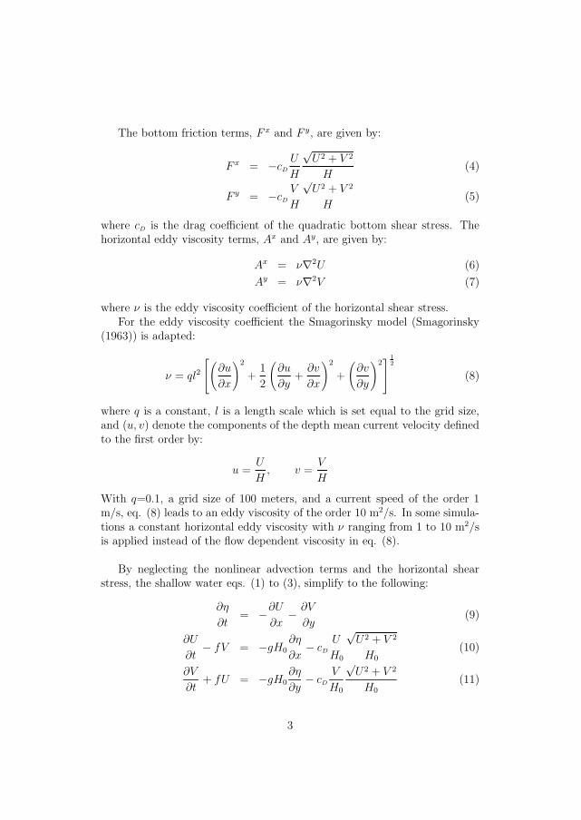
The bottom friction terms, F x and F y, are given by:

F x = −cD

U

H

√U2 + V 2

H(4)

F y = −cD

V

H

√U2 + V 2

H(5)

where cD is the drag coefficient of the quadratic bottom shear stress. Thehorizontal eddy viscosity terms, Ax and Ay, are given by:

Ax = ν∇2U (6)

Ay = ν∇2V (7)

where ν is the eddy viscosity coefficient of the horizontal shear stress.For the eddy viscosity coefficient the Smagorinsky model (Smagorinsky

(1963)) is adapted:

ν = ql2

⎡⎣(∂u

∂x

)2

+1

2

(∂u

∂y+

∂v

∂x

)2

+

(∂v

∂y

)2⎤⎦ 1

2

(8)

where q is a constant, l is a length scale which is set equal to the grid size,and (u, v) denote the components of the depth mean current velocity definedto the first order by:

u =U

H, v =

V

H

With q=0.1, a grid size of 100 meters, and a current speed of the order 1m/s, eq. (8) leads to an eddy viscosity of the order 10 m2/s. In some simula-tions a constant horizontal eddy viscosity with ν ranging from 1 to 10 m2/sis applied instead of the flow dependent viscosity in eq. (8).

By neglecting the nonlinear advection terms and the horizontal shearstress, the shallow water eqs. (1) to (3), simplify to the following:

∂η

∂t= −∂U

∂x− ∂V

∂y(9)

∂U

∂t− fV = −gH0

∂η

∂x− cD

U

H0

√U2 + V 2

H0(10)

∂V

∂t+ fU = −gH0

∂η

∂y− cD

V

H0

√U2 + V 2

H0(11)

3

This is the same set of equations as implemented in the PLN-model. Theequations were discretized on a C-grid (Mesinger and Arakawa (1976)) shownin figure 1, with a uniform spatial grid resolution �s and time step �t:

ηi,j(t +�t)− ηi,j(t)

�t= −Ui+1,j(t)− Ui,j(t)

�s− Vi,j+1(t)− Vi,j

�s(12)

Ui,j(t +�t)− Ui,j(t)

�t= fV i,j(t)− gH0

i

i,j

ηi,j(t +�t)− ηi−1,j(t +�t)

�s

−cD

Ui,j(t)

H0i

i,j

√U2

i,j(t) + V2

i,j(t)

H0i

i,j

(13)

Vi,j(t +�t)− Vi,j(t)

�t= −fU i,j(t +�t)− gH0

j

i,j

ηi,j(t +�t)− ηi,j−1(t +�t)

�s

−cD

Vi,j(t)

H0j

i,j

√U

2

i,j(t +�t) + V 2i,j(t)

H0j

i,j

(14)

where

H0i

i,j =1

2(H0i,j + H0i−1,j)

H0j

i,j =1

2(H0i,j + H0i,j−1)

V i,j =1

4(Vi,j + Vi−1,j + Vi,j+1 + Vi−1,j+1)

U i,j =1

4(Ui,j + Ui+1,j + Ui,j−1 + Ui+1,j−1)

The simulations are started from rest (η=U=V =0) and are driven byspecified surface elevation η at the open boundaries. Boundary values areeither obtained from a model covering a larger domain or by interpolatingdata from a model with coarser grid. The interior solution are adjusted tothe specified boundary conditions with the flow relaxation scheme (FRS),Martinsen and Engedahl (1987). The FRS softens the transition from anexterior solution to an interior solution by use of a grid zone where thetwo solutions dominate at each ends respectively. How a FRS zone can beimplemented in tidal models is described by Moe et al. (2002) and Moe et al.(2003). Further details about the PLN-model, are given in the same papers.

4

Ui,j

Vi,j

Hi,j Ui+1,j

Vi+1,j

Hi+1,jUi−1,j

Vi−1,j

Hi−1,j

Ui,j+1

Vi,j+1

Hi,j+1

Ui,j−1

Vi,j−1

Hi,j−1 Ui+1,j−1

Vi+1,j−1

Hi+1,j−1Ui−1,j−1

Vi−1,j−1

Hi−1,j−1

Ui−1,j+1

Vi−1,j+1

Hi−1,j+1 Ui+1,j+1

Vi+1,j+1

Hi+1,j+1

Δ s

Δ s

Figure 1: C-grid stencil with a uniform spatial grid resolution�s. The circlesdenotes grid points where both sea surface displacement, η, and depth, H, arespecified. Lines represent grid nodes for volume fluxes U and V .

3 Implementation of nonlinear terms

3.1 The total depth

The first and easiest modification of the PLN-model is to use the total depth,H , instead of the mean depth, H0. This is done by adding η to H0 after ηis calculated in every grid node, and then using H in the calculations for Uand V .

In order to study the effect of replacing H0 by H = H0 + η in the PLN-model, eqs. (12)-(14), some numerical tests have been made, see section5.1.

3.2 The nonlinear advection terms

Following the same discretization as used in the linear equations, the non-linear advection terms in eqs. (2) and (3) have been represented with thenumerical form:

Nxi,j =

1

�s

⎛⎝Ui 2

i,j

Hi,j− U

i 2

i−1,j

Hi−1,j

⎞⎠+1

�s

⎛⎝Uj

i,j+1Vi

i,j+1

Hi,j+1

− Uj

i,jVi

i,j

H i,j

⎞⎠ (15)

5

A

B

C

Figure 2: Example of the grid mesh in the coastal zone. Red and yellow linesillustrate fluxes in the coastal zone, blue in the interior domain. Blue circlesrepresent points for sea surface displacement. Green circles represent landpoints.

Nyi,j =

1

�s

⎛⎝Uj

i+1,jVi

i+1,j

Hi+1,j

− Uj

i,jVi

i,j

H i,j

) +1

�s(V

j 2

i,j

Hi,j

− Vj 2

i,j−1

Hi,j−1

⎞⎠ (16)

where

Ui

i,j =1

2(Ui+1,j + Ui,j)

Uj

i,j =1

2(Ui,j + Ui,j−1)

Vi

i,j =1

2(Vi,j + Vi−1,j)

Vj

i,j =1

2(Vi,j+1 + Vi,j)

H i,j =1

4(Hi,j + Hi−1,j + Hi,j−1 + Hi−1,j−1)

For the nearest fluxes parallel to the coastline we have used a one-sideddifference in the nonlinear advection terms. These fluxes are said to belocated in a coastal zone as illustrated in figure 2.

To include the nonlinear advection terms also for the coastal zone, ap-proximation methods must be used. The four approximation methods usedfor a straight coastline are illustrated by figure 3:

1. The nonlinear advection terms in the coastal zone, f(0), are set to zero:

f1(0) = 0

6

Number of grid cells from coastal zone0 1 2

f1(0)

f2(0)

f3(0)

f4(0)

f(1)

f(2)

Figure 3: Four methods to approximate a nonlinear advection term in thecoastal zone, fn(0), where n=1,2,3,4 represents the method listed in the text.f(1) is the value of the term one grid cell away from the coastal zone, andf(2) the value two grid cells away from the coastal zone.

2. The nonlinear advection terms in the coastal zone, f(0), equal thenonlinear advection terms in the the nearest neighbouring grid cell,f(1):

f2(0) = f(1)

3. The nonlinear advection terms in the coastal zone, f(0), equal the meanof the value of the terms in two grid points nearest to the coast, f(1)and f(2):

f3(0) =1

2(f(1) + f(2))

4. The nonlinear advection terms in the coastal zone, f(0), is determinedby a linear extrapolation of the nonlinear advection terms from twogrid cells close to the coast, f(1) and f(2):

f4(0) = f(1) +f(2)− f(1)

2− 1(0− 1) = 2f(1)− f(2)

The following describe in detail how the four methods were modified incase of more complicated coastlines:

3.2.1 Special case: channel

In a narrow channel with only one or two grid cells, the nonlinear advectionterms are set to zero as shown in figure 4.

7

2 2 2 2

2 2 2 2

2

21 1 1 1

1 1 12/2

2/1

2/1

D E

F

Figure 4: Example of a narrow channel. Red and yellow lines illustratefluxes located in the coastal zone, blue in the interior domain. Dotted linesillustrates fluxes where the nonlinear advection terms are set to zero. Bluecircles represent points for sea surface displacement. Green circles representland points.

In a channel with three grid cells, only the nonlinear advection terms inthe middle of the channel are calculated without one-sided differences. Thenonlinear advection terms in the coastal zone on each side of the channel,may be approximated using only the nonlinear advection terms in the middleof the channel. This is indicated with ’1’ in figure 4.

If the nonlinear advection terms in a coastal zone are approximated usingtwo or more nonlinear advection terms in one direction, this in indicated with’2’ in figure 4.

3.2.2 Special case: corners

A flux is said to be in the coastal zone near a corner if the parallel neigh-bouring fluxes in two directions is located in the water outside the coastalzone.

The nonlinear advection term for a flux in the coastal zone near a corneris approximated as the mean value of the approximation in these directions.

The flux marked with ’2/2’ in figure 4 and all the fluxes illustrated by yel-low lines in figure 2 may use two nonlinear advection terms in each directionto approximate the nonlinear advection term in the coastal zone.

The fluxes marked with ’2/1’ in figure 4 may use two nonlinear advectionterms in one direction and one term in another direction to approximate theterms in the coastal zone.

8

3.2.3 Implementation of the nonlinear advection terms

Before expressing the full equations for the nonlinear advection terms, fournew parameters are defined1. Zx

i,j and Zyi,j denote whether the fluxes are

located in the coastal zone or in the interior domain:

Zxi,j =

{0, if the flux Ui,j lies in the coastal zone or next to a land node1, if the flux Ui,j lies in the water outside the coastal zone

Zyi,j =

{0, if the flux Vi,j lies in the coastal zone or next to a land node1, if the flux Vi,j lies in the water outside the coastal zone

and Cxi,j and Cy

i,j denote the coast type for the fluxes in the coastal zone:

Cxi,j =

⎧⎪⎪⎪⎨⎪⎪⎪⎩0, if the flux Ui,j lies in the water outside the coastal zone

or next to a land node1, if the flux Ui,j lies in a coastal zone, but not near a corner

0.5, if the flux Ui,j lies in a coastal zone near a corner

Cyi,j =

⎧⎪⎪⎪⎨⎪⎪⎪⎩0, if the flux Vi,j lies in the water outside the coastal zone

or next to a land node1, if the flux Vi,j lies in a coastal zone, but not near a corner

0.5, if the flux Vi,j lies in a coastal zone near a corner

First the nonlinear advection terms are calculated in every grid cell, usingeq. (15) and (16). Then the terms are completed by approximation in thecoastal zone using one of the four methods:

Method 1:

Nxi,j (1) = Zx

i,j Nxi,j (17)

Nyi,j (1) = Zy

i,j Nyi,j (18)

Method 2:

Nxi,j (2) = Zx

i,j Nxi,j + Cx

i,j (Nxi−1,j + Nx

i+1,j + Nxi,j−1 + Nx

i,j+1) (19)

Nyi,j (2) = Zy

i,j Nyi,j + Cy

i,j (Nyi−1,j + Ny

i+1,j + Nyi,j−1 + Ny

i,j+1) (20)

Method 3:

Nxi,j (3) = Zx

i,j Nxi,j + 1

2Cx

i,j [ (2− Zxi−2,j) Nx

i−1,j + Zxi−1,j Nx

i−2,j

+(2− Zxi+2,j) Nx

i+1,j + Zxi+1,j Nx

i+2,j

+(2− Zxi,j−2) Nx

i,j−1 + Zxi,j−1 Nx

i,j−2

+(2− Zxi,j+2) Nx

i,j+1 + Zxi,j+1 Nx

i,j+2 ]

(21)

1Note that Zx is called uinl in the model code, Zy is called vinl, Cx is called uik, andCy is called vik.

9

Nyi,j (3) = Zy

i,j Nyi,j + 1

2Cy

i,j [ (2− Zyi−2,j) Ny

i−1,j + Zyi−1,j Ny

i−2,j

+(2− Zyi+2,j) Ny

i+1,j + Zyi+1,j Ny

i+2,j

+(2− Zyi,j−2) Ny

i,j−1 + Zyi,j−1 Ny

i,j−2

+(2− Zyi,j+2) Ny

i,j+1 + Zyi,j+1 Ny

i,j+2 ]

(22)

Method 4:

Nxi,j (4) = Zx

i,j Nxi,j + Cx

i,j [ (1 + Zxi−2,j) Nx

i−1,j − Zxi−1,j Nx

i−2,j

+(1 + Zxi+2,j) Nx

i+1,j − Zxi+1,j Nx

i+2,j

+(1 + Zxi,j−2) Nx

i,j−1 − Zxi,j−1 Nx

i,j−2

+(1 + Zxi,j+2) Nx

i,j+1 − Zxi,j+1 Nx

i,j+2 ]

(23)

Nyi,j (4) = Zy

i,j Nyi,j + Cy

i,j [ (1 + Zyi−2,j) Ny

i−1,j − Zyi−1,j Ny

i−2,j

+(1 + Zyi+2,j) Ny

i+1,j − Zyi+1,j Ny

i+2,j

+(1 + Zyi,j−2) Ny

i,j−1 − Zyi,j−1 Ny

i,j−2

+(1 + Zyi,j+2) Ny

i,j+1 − Zyi,j+1 Ny

i,j+2 ]

(24)

Note that for the fluxes in the water outside the coastal zone, eq. (17) to(24) become:

Nxi,j (1)→(4) = Nx

i,j Nyi,j (1)→(4) = Ny

i,j

since Zxi,j = Zy

i,j = 1 and Cxi,j = Cy

i,j = 0 in the water outside the coastalzone.

For our model setup the first and the last method proceed to be the moststable. Therefore section 5 only presents results from simulations with thesetwo approximation methods.

Example A The flux, Vi,j, marked ’A’ in figure 2 is located in the coastalzone, and has water outside the coastal zone, in one direction. Therefore thenonlinear advection term is approximated in one direction. Eqs. (20), (22)and (24) become:

Nyi,j (2) = Ny

i−1,j

Nyi,j (3) =

1

2(Ny

i−1,j + Nyi−2,j)

Nyi,j (4) = 2Ny

i−1,j −Nyi−2,j

10

Example B The flux, Ui,j , marked ’B’ in figure 2 is located in the coastalzone near a corner. Since the flux has water outside the coastal zone intwo directions, the nonlinear advection term is approximated in these twodirections. Eqs. (19), (21) and (23) become:

Nxi,j (2) =

1

2(Nx

i+1,j + Nxi,j+1)

Nxi,j (3) =

1

4(Nx

i+1,j + Nxi+2,j + Nx

i,j+1 + Nxi,j+2)

Nxi,j (4) =

1

2(2Nx

i+1,j −Nxi+2,j + 2Nx

i,j+1 −Nxi,j+2)

Example C The flux, Vi,j, marked ’C’ in figure 2 is located in the coastalzone, and has water outside the coastal zone, in one direction. The nonlinearadvection term is approximated in the same way as the flux in example A:Eqs. (20), (22) and (24) become:

Nyi,j (2) = Ny

i,j+1

Nyi,j (3) =

1

2(Ny

i,j+1 + Nyi,j+2)

Nyi,j (4) = 2Ny

i,j+1 −Nyi,j+2

Example D The flux, Ui,j, marked ’D’ in figure 4 is located in the coastalzone, and has water outside the coastal zone, in one direction. Since onlyone of the two nearest fluxes in that direction is located outside a coastalzone, only one grid cell is used in all the approximation methods. Eqs. (19),(21) and (23) become:

Nxi,j (2) = Nx

i,j (3) = Nxi,j (4) = Nx

i+1,j

Example E The flux Ui,j , marked ’E’ in figure 4 is located in the coastalzone, but does not have any neighbouring fluxes in water outside the coastalzone. Therefore this non-zero advection term is set to zero in all four ap-proximation methods. Eqs. (19), (21) and (23) become:

Nxi,j (2) = Nx

i,j (3) = Nxi,j (4) = 0

Example F The flux, Ui,j , marked ’F’ in figure 4 is located in the coastalzone near a corner. Since the flux has water outside the coastal zone intwo directions, the nonlinear advection term is approximated in these two

11

directions. In one of these direction, the flux two grid cells from the fluxmarked ’E’ is located in a coastal zone. Eqs. (19), (21) and (23) become:

Nxi,j (2) =

1

2(Nx

i+1,j + Nxi,j+1)

Nxi,j (3) =

1

4(Nx

i+1,j + Nxi+2,j + 2Nx

i,j+1)

Nxi,j (4) =

1

2(2Nx

i+1,j −Nxi+2,j + Nx

i,j+1)

3.3 Horizontal eddy viscosity

Following the same discretization as used in the original PLN-model, thehorizontal eddy viscosities in eqs. (6) and (7) have the numerical form:

Axi,j =

ν

(�s)2(Ui+1,j + Ui−1,j + Ui,j+1 + Ui,j−1 − 4Ui,j) (25)

Ayi,j =

ν

(�s)2(Vi+1,j + Vi−1,j + Vi,j+1 + Vi,j−1 − 4Vi,j) (26)

The PLN-model used in this report is without horizontal eddy viscosity.In order to make our nonlinear simulations stable, sufficient horizontal eddyviscosity has to be included. This will be discussed further in section 5.1.

Since central differencing cannot be used in the coastal zone, the horizon-tal eddy viscosity cannot be calculated to the same order of accuracy in thecoastal zone as in the interior domain. The four suggested approximationmethods used for the nonlinear advection terms, have also been evaluated forthe eddy viscosity. The most stable method was to set the horizontal eddyviscosity to zero in the coastal zone. After calculating the various terms in-cluded in the horizontal eddy viscosity in the interior domain, the scheme iscompleted by setting these terms equal to zero in the coastal zone:

Axi,j = Zx

i,j Axi,j

Ayi,j = Zy

i,j Ayi,j

If the horizontal eddy viscosity is included closer than two grid cells fromthe FRS zone, the simulations become unstable in less than 20 hours simu-lated time. Therefore neither the horizontal eddy viscosity nor the nonlinearadvection terms are included closer than two grid cells from the FRS zone.

3.4 Bottom shear stress

According to Crean et al. (1995) the bottom shear stress dominates thehorizontal eddy viscosity near the coast. Crean et al. therefore set the

12

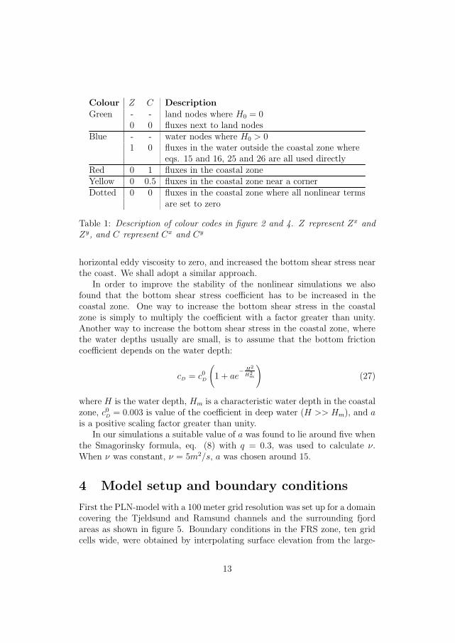
Colour Z C DescriptionGreen - - land nodes where H0 = 0

0 0 fluxes next to land nodesBlue - - water nodes where H0 > 0

1 0 fluxes in the water outside the coastal zone whereeqs. 15 and 16, 25 and 26 are all used directly

Red 0 1 fluxes in the coastal zoneYellow 0 0.5 fluxes in the coastal zone near a cornerDotted 0 0 fluxes in the coastal zone where all nonlinear terms

are set to zero

Table 1: Description of colour codes in figure 2 and 4. Z represent Zx andZy, and C represent Cx and Cy

horizontal eddy viscosity to zero, and increased the bottom shear stress nearthe coast. We shall adopt a similar approach.

In order to improve the stability of the nonlinear simulations we alsofound that the bottom shear stress coefficient has to be increased in thecoastal zone. One way to increase the bottom shear stress in the coastalzone is simply to multiply the coefficient with a factor greater than unity.Another way to increase the bottom shear stress in the coastal zone, wherethe water depths usually are small, is to assume that the bottom frictioncoefficient depends on the water depth:

cD = c0D

(1 + ae

− H2

H2m

)(27)

where H is the water depth, Hm is a characteristic water depth in the coastalzone, c0

D = 0.003 is value of the coefficient in deep water (H >> Hm), and ais a positive scaling factor greater than unity.

In our simulations a suitable value of a was found to lie around five whenthe Smagorinsky formula, eq. (8) with q = 0.3, was used to calculate ν.When ν was constant, ν = 5m2/s, a was chosen around 15.

4 Model setup and boundary conditions

First the PLN-model with a 100 meter grid resolution was set up for a domaincovering the Tjeldsund and Ramsund channels and the surrounding fjordareas as shown in figure 5. Boundary conditions in the FRS zone, ten gridcells wide, were obtained by interpolating surface elevation from the large-

13

Hinnøya

Narvik

Evenskjær

Tysfjorden

Ofotfjorden

Vagsfjorden

Figure 5: The model domain covering the Tjeldsund and Ramsund channelsand the surrounding fjord area. The red dots mark stations for output of timeseries.

scale PLN-model for the area around the Lofoten Islands with 500 meter gridresolution (Moe et al. (2002)).

The high resolution depth matrix based on new bathymetric surveys ofthe model domain was not ready during this work. Therefore a test depthmatrix with 100 meter grid grid resolution was constructed by interpolatingfrom the depth matrix with 500 meter grid. Additional simulations will beconducted when a new depth matrix with 50 and 25 meter grid resolutionbecomes available.

Next the PLN-model with a 100 meter grid resolution was set up for asub domain covering only the Tjeldsund and Ramsund channels as shown infigure 6. The boundary conditions in the FRS zone were obtained from themodel covering the whole domain in figure 5. The results of the simulations

14

Tjeldsund

Sandtorgstraumen

Steinlandstraumen

Spannbogstraumen

Ballstadstraumen

Tjeldøya

Tjeldsund

Ramsund

Ofotfjorden

st.1st.2

st.3

st.4

st.5

Figure 6: The model domain for the full nonlinear model. The red dots markthe five stations for output of time series, st.1 - st.5, discussed in this report.

for the two model domains in figure 5 and 6 were compared. Only minordifferences in the current and the surface elevation were detected.

Then the full nonlinear model was set up for the domain in figure 6 withthe same boundary conditions as for the PLN-model for the same domain.For the test depth matrix the mean water depth in the coastal zone, withspecial treatment of the nonlinear advection terms, was 5.6 meters. Themaximum water depth in the coastal zone was 29.5 meters. The referencedepth Hm in eq. (27) was therefore set Hm=5.6 m.

The tidal model reported here is driven only by surface amplitude andphase for the M2 component at the open boundaries. The boundary forc-ing started from rest and increased in time with a ramping function, (1−exp(−σt)). A value of σ = 4.6 × 10−5s−1 has been used which implies fulleffect of boundary conditions after about 12 hours. This is similar to whatwas used for the PLN-model.

For every 180 seconds, surface elevation, current amplitude and phase atthe output-stations were stored. Time series for the stations showed somenoise due to the transient start. After 50 hours, full fields for current and

15

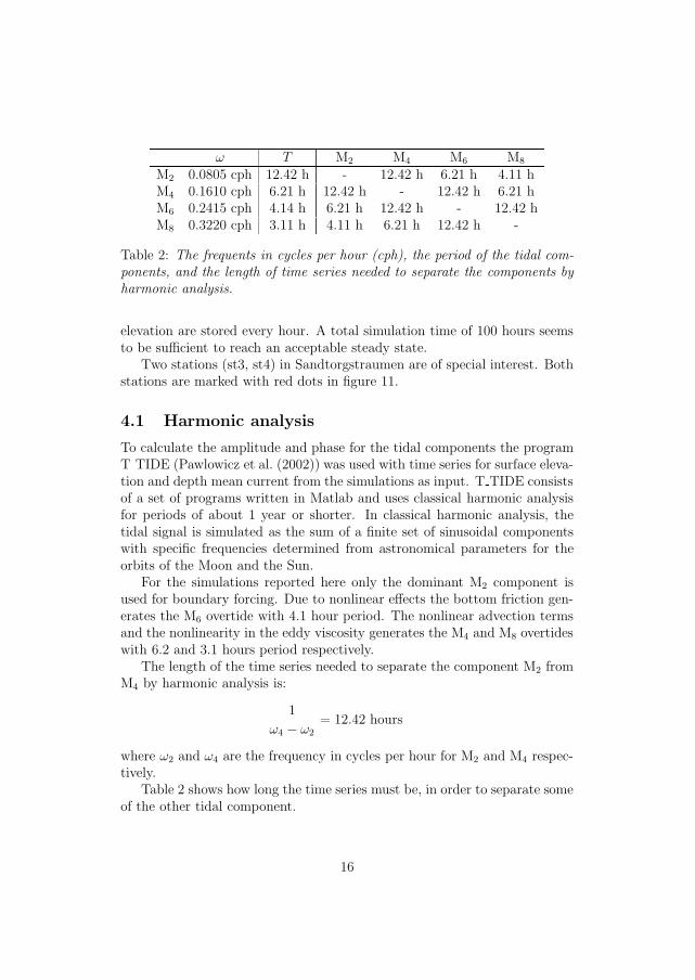
ω T M2 M4 M6 M8

M2 0.0805 cph 12.42 h - 12.42 h 6.21 h 4.11 hM4 0.1610 cph 6.21 h 12.42 h - 12.42 h 6.21 hM6 0.2415 cph 4.14 h 6.21 h 12.42 h - 12.42 hM8 0.3220 cph 3.11 h 4.11 h 6.21 h 12.42 h -

Table 2: The frequents in cycles per hour (cph), the period of the tidal com-ponents, and the length of time series needed to separate the components byharmonic analysis.

elevation are stored every hour. A total simulation time of 100 hours seemsto be sufficient to reach an acceptable steady state.

Two stations (st3, st4) in Sandtorgstraumen are of special interest. Bothstations are marked with red dots in figure 11.

4.1 Harmonic analysis

To calculate the amplitude and phase for the tidal components the programT TIDE (Pawlowicz et al. (2002)) was used with time series for surface eleva-tion and depth mean current from the simulations as input. T TIDE consistsof a set of programs written in Matlab and uses classical harmonic analysisfor periods of about 1 year or shorter. In classical harmonic analysis, thetidal signal is simulated as the sum of a finite set of sinusoidal componentswith specific frequencies determined from astronomical parameters for theorbits of the Moon and the Sun.

For the simulations reported here only the dominant M2 component isused for boundary forcing. Due to nonlinear effects the bottom friction gen-erates the M6 overtide with 4.1 hour period. The nonlinear advection termsand the nonlinearity in the eddy viscosity generates the M4 and M8 overtideswith 6.2 and 3.1 hours period respectively.

The length of the time series needed to separate the component M2 fromM4 by harmonic analysis is:

1

ω4 − ω2

= 12.42 hours

where ω2 and ω4 are the frequency in cycles per hour for M2 and M4 respec-tively.

Table 2 shows how long the time series must be, in order to separate someof the other tidal component.

16

Bottom drag coefficient, cD

depend on depths multiplied with neq. 27 in coastal zone

eddy viscosity coefficient, ν a = 2 a = 3 n = 4 n = 10constant ν = 3 m2/s unstable unstable unstable unstable

ν = 4 m2/s - - - stableν = 5 m2/s - - unstable -ν = 6 m2/s - - stable -ν = 10 m2/s - unstable - -ν = 15 m2/s unstable stable stable stable

Smagorinsky q = 0.1 unstable unstable unstable unstableeq. 8 q = 0.2 stable stable unstable stable

q = 0.3 - - stable -q = 5 - - stable -q = 10 stable stable unstable stable

Table 3: The stability after 100 hours of full nonlinear simulations with dif-ferent choices of friction coefficients, and the nonlinear advection terms ex-trapolated in the coastal zone.

5 Results

5.1 Currents and volume fluxes

Strong currents occur in Sandtorgstraumen north-east of Tjeldøya, in Stein-landsstraumen up north in Tjeldsundet and in Ballstadstraumen north ofTjeldøya. In Spannbogstraumen in Ramsundet east of Tjeldøya the currentsare weaker, but since the water depths are small and the channel is narrow,the currents is considerable even here.

Among the many difficulties with nonlinear simulations, a crucial choiceis to balance the amount of friction. With too little friction, the simula-tions become unstable, and too much friction, leads to an unrealistic strongdamping of the current.

Table 3 shows which choices of ν and cD that are suitable when thenonlinear advection terms are extrapolated in the coastal zone. Note thatwhen the Smagorinsky formula, eq. (8), is used to calculate the eddy viscositycoefficient, the simulations are stable only for an interval of q.

This section presents results from the five full nonlinear simulations listedin table 4. For each of these simulations, the coefficients cD and ν are chosenas small as possible for maintaining stable solutions for 100 hours simulationtime. If the coefficients are chosen smaller, the simulations become unstable.

17

Horizontal eddy Bottom drag nonlinear advectionRun viscosity coefficient coefficient terms in coastal zone

1 q = 0.3 in eq. (8) a = 3 in eq. (27) extrapolated2 ν = 6 m2/s, constant x4 in coastal zone extrapolated3 q = 0.3 in eq. (8) x4 in coastal zone extrapolated4 ν = 4 m2/s, constant x4 in coastal zone set to zero5 q = 0.1 in eq. (8) set to zero

Table 4: The five full nonlinear simulations.

These limits depend on the topography, the grid length, location, initialconditions, boundary conditions, and current magnitude.

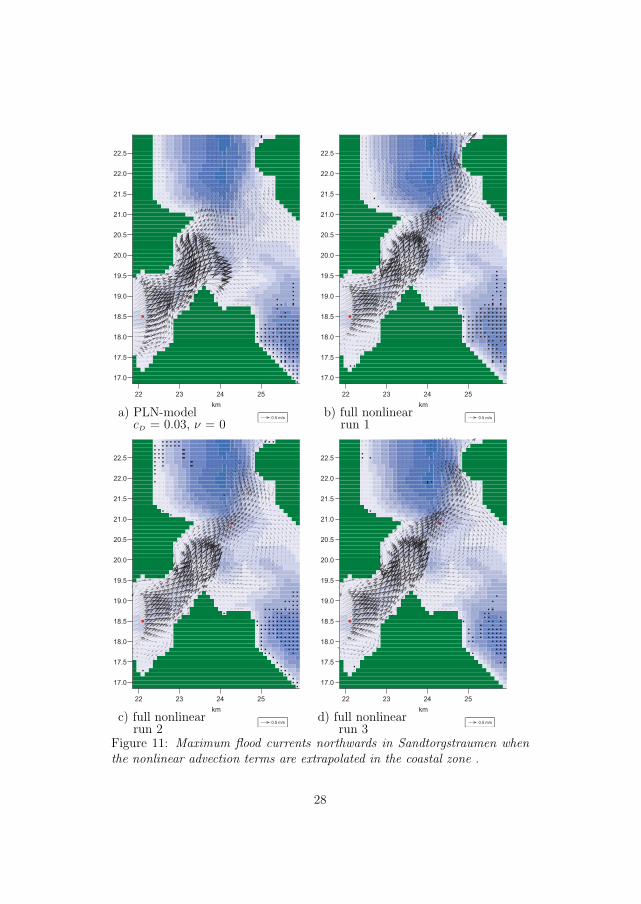
Figure 11 to 18 show plots which are generated from PLN-simulationsand the five full nonlinear simulations listed in table 4.

Figure 11 and 12 show the northern part of Sandtorgstraumen at the timeof maximum flow northwards. Figure 11 shows results from one PLN modelsimulation and the three full nonlinear simulation where the nonlinear advec-tion terms are extrapolated in the coastal zone. Figure 12 shows results fromthe two full nonlinear simulation where the nonlinear advection terms are setto zero in the coastal zone. Plots from the same simulations are shown formaximum flow southwards in Sandtorgstraumen, and for Steinlandsstraumenin figure 13 to 18.

The most important differences between the simulations with the PLN-model and with the full nonlinear model are the formation of intensifiedjets and eddies on various scales as shown in figure 11 to 18. Of coursethis is not unexpected, but we have been able to demonstrate how sensitivethese current features are to various methods of implementing the nonlinearadvection terms.

All the simulations with the full nonlinear model show an intensified jetflow and eddy structures on each side of the jet north-east of Sandtorgstrau-men. The eddy structures have slightly different forms. A closer look atthe plots from the full nonlinear simulations reveals currents in the oppositedirection close to land in some places. This effect is probably due to theincreased bottom friction applied in the coastal zone. This effect is strongerwhen the nonlinear advection terms are extrapolated in the coastal zone,compared to when the nonlinear advection terms are set to zero.

When the nonlinear advection terms are extrapolated in the coastal zone,and the horizontal friction coefficient, ν, is calculated using Smagorinskyformula, eq. (8), very strong currents occur close to land on the east sideof the channel in the northern part of the domain as shown in figure 15b.

18

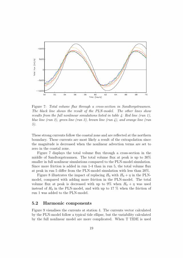
Figure 7: Total volume flux through a cross-section in Sandtorgstraumen.The black line shows the result of the PLN-model. The other lines showresults from the full nonlinear simulations listed in table 4: Red line (run 1),blue line (run 2), green line (run 3), brown line (run 4), and orange line (run5).

These strong currents follow the coastal zone and are reflected at the northernboundary. These currents are most likely a result of the extrapolation sincethe magnitude is decreased when the nonlinear advection terms are set tozero in the coastal zone.

Figure 7 displays the total volume flux through a cross-section in themiddle of Sandtorgstraumen. The total volume flux at peak is up to 30%smaller in full nonlinear simulations compared to the PLN-model simulation.Since more friction is added in run 1-4 than in run 5, the total volume fluxat peak in run 5 differ from the PLN-model simulation with less than 20%.

Figure 8 illustrates the impact of replacing H0 with H0 + η in the PLN-model, compared with adding more friction in the PLN-model. The totalvolume flux at peak is decreased with up to 9% when H0 + η was usedinstead of H0 in the PLN-model, and with up to 17 % when the friction ofrun 1 was added to the PLN-model.

5.2 Harmonic components

Figure 9 visualises the currents at station 4. The currents vector calculatedby the PLN-model follow a typical tide ellipse, but the variability calculatedby the full nonlinear model are more complicated. When T TIDE is used

19

Figure 8: Total volume flux through a cross-section in Sandtorgstraumen.The black line shows results of the PLN-model, and the red line shows resultsfrom the PLN-model modified with H = H0 + η instead of H0. Both withconstant bottom friction coefficient and no horizontal eddy viscosity.The blue line shows results from run 1 in table 4. The green line shows resultsfrom the PLN-model with the same friction choices as in the full nonlinearsimulation.

to analyse the currents at station 4, it leads to a rather large rest currenti.e. the difference between simulated currents and the currents T TIDErecognises as tidal currents. This is clearly seen from figure 10. The restcurrent is stable and periodic. The period of the rest current is from 1-4hours and the amplitude is about 40 percent of the M2 tidal component.The magnitude of the rest current vary much from one station to another.

Table 5 and 6 show the calculated harmonic constants for the tidal com-ponents, sea level and current, for station 3 and 4. As the tables show, theamplitudes for M4 and M6 are, as expected, significantly larger in the fullnonlinear simulation compared to the PLN-simulation.

The observed sea level amplitude and phase for the actual tidal compo-nents (Lynge, 2004) are shown in table 7. Table 7 also shows results fromthe PLN-model, and table 8 shows results from the full nonlinear model forthe stations closest to the observed stations.

The simulated sea level amplitude for M2 agrees well with the observedamplitude. The observed sea level amplitude for M4 is somewhat larger thanthe simulated amplitudes. As expected the full nonlinear model leads to

20

−0.05 −0.04 −0.03 −0.02 −0.01 0 0.01 0.02 0.03 0.04 0.05−0.4

−0.3

−0.2

−0.1

0

0.1

0.2

0.3

0.4

Current in x−direction (m/s)

Cur

rent

in y

−dire

ctio

n (m

/s)

−0.1 0 0.1 0.2 0.3 0.4 0.5 0.6−0.4

−0.3

−0.2

−0.1

0

0.1

0.2

0.3

0.4

0.5

0.6

Current in x−direction (m/s)

Cur

rent

in y

−dire

ctio

n (m

/s)

a) b)Figure 9: Currents at station 4 in a) a PLN-simulation, and b) the full non-linear simulation with run 5. The blue curve represents the simulated current,green the current that T Tide recognised as tide-currents, red represents therest, and the dotted curve represents the tidal ellipse for M2.

larger amplitudes for M4 than the PLN-model. The highest simulated sealevel amplitude for M4 is found when Smagorinsky formula is used insteadof a constant eddy viscosity coefficient, and when the nonlinear advectionterms are extrapolated in the coastal zone, instead of setting these terms tozero in the coastal zone. The sea level amplitude for M6 is larger for the fullnonlinear model than observed. This indicate that to much bottom frictionis included.

21

st 3 PLN-model Full nonlinear (run 5)const. hη [cm] gη [deg] hη [cm] gη [deg]M2 83.94 ± 0.001 339.68 ± 0.05 84.94 ± 0.000 4.43 ± 0.03M4 1.60 ± 0.000 205.42 ± 1.24M6 0.64 ± 0.001 49.77 ± 7.32 0.85 ± 0.000 109.56 ± 2.41

st 4 PLN-model Full nonlinear (run 5)const. hη [cm] gη [deg] hη [cm] gη [deg]M2 74.20 ± 0.000 340.27 ± 0.04 75.11 ± 0.000 5.79 ± 0.01M4 0.50 ± 0.000 347.40 ± 1.85M6 0.67 ± 0.000 122.80 ± 3.82 1.04 ± 0.000 160.95 ± 0.99

Table 5: The calculated harmonic constants for see level amplitude, hη, andphase relative Greenwich, gη, at station 3 and 4.

6 Concluding remarks

Different strategies for including the nonlinear advection terms in tidal sim-ulations are tested and results of simulations are presented. Near the coastthe nonlinear advection terms can not be calculated with central differencingin the same manner as in the interior water. We have found that by extrap-olating the nonlinear advection terms into a narrow zone near the coast thesimulations are less stable than when the nonlinear advection terms are set tozero in this zone. Extrapolation leads however to stronger nonlinear effectsin the interior domain manifested by higher amplitudes of the overtides.

To make our full nonlinear tidal simulations stable, sufficient horizontaleddy viscosity and bottom shear stress had to be included. If the nonlin-ear advection terms are extrapolated in the coastal zone, a constant hori-zontal eddy viscosity coefficient of 6 m2/s is proved to be sufficient if thebottom shear stress is increased by a factor of 4 near the coast. When theSmagorinsky formula is used for the horizontal eddy viscosity coefficient, avalue of q = 0.3 is sufficient if the bottom stress coefficient either is increasedfour times near the coast or exponentially increased with depth with a factora = 3, (eq. 27). If the nonlinear advection terms are set to zero in the coastalzone, less friction need to be included. A constant horizontal eddy viscositycoefficient of 4 m2/s is proved to be sufficient if the bottom stress coefficientis increased by a factor of 4 near the coast. And when the Smagorinsky for-mula is used for the horizontal eddy viscosity coefficient, a value of q = 0.1is sufficient without increasing the bottom stress coefficients.

We advice to set the nonlinear advection terms to zero in a narrow zone

22

st 3 PLN-model Full nonlinear (run 5)A B θ gc A B θ gc

const. [cm/s] [cm/s] [deg] [deg] [cm/s] [cm/s] [deg] [deg]M2 118.8 -3.9 27.1 28.4 115.3 -0.5 28.3 18.3M4 6.6 -0.3 21.1 16.3M6 6.0 -1.0 20.4 339.6 8.0 -0.6 18.2 305.2M8 0.7 -0.4 32.7 307.4

st 4 PLN-model Full nonlinear (run 5)A B θ gc A B θ gc

const. [cm/s] [cm/s] [deg] [deg] [cm/s] [cm/s] [deg] [deg]M2 32.1 -3.4 93.5 46.7 35.3 3.0 76.5 29.0M4 9.0 2.5 46.9 43.1M6 0.13 -0.1 94.0 335.6 7.0 -0.1 27.3 34.3M8 3.9 0.9 24.1 23.8

Table 6: The calculated parameters of current ellipse at station 3 and 4.Major and minor half axis denoted A and B respectively. Orientation, θ,of major axis relative east, and phase, gc, degrees relative Greenwich, (east:gc = 0o, south: gc = 0o, etc.).

near the coast, use Smagorinsky formula to calculate the horizontal eddyviscosity coefficient, and, if necessary, increase the bottom stress coefficientexponentially with depth (eq. 27). Note that when the Smagorinsky formulais used for the horizontal eddy viscosity coefficient, and sufficient bottomshear stress is included, the simulations are stable only for an interval of q.

For the 100 meter grid used here depth is interpolated from a depthmatrix with 500 meter grid. More simulation tests will be conducted whena new depth matrix with grid resolution of 25 and 50 meter is constructedfrom new bathymetric data.

When a full nonlinear simulation is run with a new depth matrix weexpect that the coefficients of both the bottom friction and the horizontaleddy viscosity have to be modified in order to make the simulations stablewith a realistic amount of damping. The results presented in this reportprovide a guidance for how friction has to be adjusted.

23

OBSERVED M2 M4 M6

h g [deg] h [cm] g [deg] h [cm] g [deg][cm] g [deg] h [cm] g [deg] h [cm] g [deg]

Lødingen 96.3 334.1 4.8 276.2 0.9 341.9Ramsund 97.9 334.3 5.2 276.4 1.0 346.7Fjelldal 87.5 340.0 2.5 285.1 0.7 4.1Evenskjær 73.7 341.2 1.2 251.1 0.3 36.3PLN-MODEL with cD = 0.03, ν = 0station 1 95.8 335.4 - - - -station 2 97.6 335.6 - - - -station 3 83.9 339.7 - - 0.6 49.8station 4 74.2 340.3 - - 0.7 122.8station 5 73.8 340.6 - - 0.7 118.9

Table 7: Observed and simulated amplitude and phase for sea level (PLN-model). Lødingen is located near station 1, Ramsund is located near station2, Fjelldal near station 3, and Evenskjær is located between station 4 and 5.

References

P.B. Crean, T.S. Murty, and J.A. Stronach. Mathematical Modelling of Tidesand Estuarine Circulation. Springer-Verlag, N.Y., 1988

B. Gjevik. Model simulations of tides and shelf waves along the shelves ofthe Norwegian-Greenland-Barents Seas. Modelling Marine Systems, Vol.I,p. 187-219. Ed. A.M. Davies, CRC Press Inc. Boca Raton, Florida, 1990.

B. Gjevik, E. Nøst, T. Straume. Model simulations of the tides in the BarentsSea. J. Geophysical Res., Vol. 99, No C2, 3337–3350, 1994.

B. Gjevik, D. Hareide, B.K. Lynge, A. Ommundsen, J.H. Skailand, andH.B. Urheim. Implementation of high resolution tidal current fields in elec-tronic navigational chart systems. Preprint Series, Department of Mathe-matics, University of Oslo. ISSN 0809-4403, 2004.

B.K. Lynge Water level observations from Tjeldsundet. January-March 2004.Norwegian Hydrographic Service, report nr. DAF 04-2, 2004.

E.A. Martinsen, and H. Engedahl. Implementation and testing of a lateralboundary scheme as an open boundary condition in a barotropic oceanmodel. Coastal Engineering, Vol. 11, 603–627, 1987.

24

F. Mesinger, and A. Arakawa. Numerical Methods Used in AtmosphericModels. GARP Publications Series, No.17. 64pp, 1976.

H. Moe, A. Ommundsen, and B. Gjevik. A high resolution tidal model forthe area around the Lofoten Islands, Northern Norway. Continental ShelfResearch 22, 485-504, 2002.

H. Moe, B. Gjevik, and A. Ommundsen. A high resolution tidal modelfor the coast of Møre and Trøndelag, Mid-Norway. Norwegian journal ofGeography, Vol. 57, 65-82. Oslo. ISSN 0029-1951, 2003.

S. Orre, E. Akervik, and B. Gjevik. Analysis of current and sea level observa-tions from Trondheimsleia. Preprint Series, Department of Mathematics,University of Oslo. ISSN 0809-4403, 2004.

R. Pawlowicz, B. Beardsley, and S. Lentz. Classical Tidal Harmonic AnalysisIcluding Error Estimated in MATLAB using T TIDE. Computers andGeosciences, 28, 929-937, 2002.

J. Smagorinsky. General circulation experiments with the primitive equa-tions. Monthly Rewiew 91 (1), 99-164, 1963.

25

SIMULATED M2 M4 M6

full nonlinear h [cm] g [deg] h [cm] g [deg] h [cm] g [deg]Run 1station 1 96.2 335.4 - - - -station 2 83.0 341.7 4.3 157.1 1.4 16.7station 3 86.9 340.6 2.5 160.7 1.3 9.7station 4 76.9 342.5 1.6 216.8 1.7 63.3station 5 76.8 342.5 1.6 212.8 1.7 64.5Run 2station 1 96.1 335.4 - - 0.1 311.4station 2 97.5 335.7 - - 0.1 270.2station 3 85.1 340.5 1.9 156.0 1.1 30.6station 4 76.2 342.2 0.6 247.9 1.4 67.1station 5 76.0 342.3 0.6 253.2 1.3 65.2Run 3station 1 96.2 335.4 - - - -station 2 97.8 335.5 - - - -station 3 85.5 340.5 2.1 157.4 1.1 29.5station 4 76.4 342.2 1.0 219.9 1.4 69.2station 5 76.2 342.2 0.9 229.5 1.4 65.7Run 4station 1 96.1 335.4 - - - -station 2 97.5 335.7 - - - -station 3 84.8 340.4 1.7 151.8 1.0 36.9station 4 76.2 342.1 0.4 257.4 1.2 69.4station 5 76.1 342.3 0.3 286.1 1.3 98.0Run 5station 1 96.1 359.8 0.1 111.4 1.3 25.3station 2 75.4 5.8 0.4 359.9 1.3 157.1station 3 84.9 4.4 1.6 205.4 0.8 109.6station 4 75.1 5.8 0.5 347.4 1.0 160.1station 5 75.1 5.7 0.5 342.1 1.1 164.0

Table 8: Simulated amplitude and phase for sea level from the full nonlinearmodel. For further explanations see legend table 7

26

20 30 40 50 60 70 80 90 100 1100

0.05

0.1

0.15

0.2

0.25

0.3

0.35

Time (hours)

Cur

rent

(m/s

)

a) PLN-model

20 30 40 50 60 70 80 90 100 1100

0.1

0.2

0.3

0.4

0.5

0.6

0.7

Time (hours)

Cur

rent

(m/s

)

b) full nonlinear, run 2

20 30 40 50 60 70 80 90 100 1100

0.1

0.2

0.3

0.4

0.5

0.6

0.7

0.8

Time (hours)

Cur

rent

(m/s

)

c) full nonlinear, run 5

Figure 10: Harmonic analysis of the current at station 4. The blue curverepresents the simulated current, green the current that T Tide recognized astide-currents and red the rest current.

27

22 23 24 25km

17.0

17.5

18.0

18.5

19.0

19.5

20.0

20.5

21.0

21.5

22.0

22.5

0.5 m/s

22 23 24 25km

17.0

17.5

18.0

18.5

19.0

19.5

20.0

20.5

21.0

21.5

22.0

22.5

0.5 m/s

22 23 24 25km

17.0

17.5

18.0

18.5

19.0

19.5

20.0

20.5

21.0

21.5

22.0

22.5

0.5 m/s

22 23 24 25km

17.0

17.5

18.0

18.5

19.0

19.5

20.0

20.5

21.0

21.5

22.0

22.5

0.5 m/s

a) PLN-model b) full nonlinearcD = 0.03, ν = 0 run 1

c) full nonlinear d) full nonlinearrun 2 run 3

Figure 11: Maximum flood currents northwards in Sandtorgstraumen whenthe nonlinear advection terms are extrapolated in the coastal zone .

28

22 23 24 25km

17.0

17.5

18.0

18.5

19.0

19.5

20.0

20.5

21.0

21.5

22.0

22.5

0.5 m/s

22 23 24 25km

17.0

17.5

18.0

18.5

19.0

19.5

20.0

20.5

21.0

21.5

22.0

22.5

0.5 m/sa) full nonlinear b) full nonlinear

run 4 run 5Figure 12: Maximum flood currents northwards in Sandtorgstraumen whenthe nonlinear advection terms are set to zero in the coastal zone.

29

22 23 24 25km

17.0

17.5

18.0

18.5

19.0

19.5

20.0

20.5

21.0

21.5

22.0

22.5

0.5 m/s

22 23 24 25km

17.0

17.5

18.0

18.5

19.0

19.5

20.0

20.5

21.0

21.5

22.0

22.5

0.5 m/s

22 23 24 25km

17.0

17.5

18.0

18.5

19.0

19.5

20.0

20.5

21.0

21.5

22.0

22.5

0.5 m/s

22 23 24 25km

17.0

17.5

18.0

18.5

19.0

19.5

20.0

20.5

21.0

21.5

22.0

22.5

0.5 m/s

a) PLN-model b) full nonlinearcD = 0.03, ν = 0 run 1

c) full nonlinear d) full nonlinearrun 2 run 3

Figure 13: Maximum ebb currents southwards in Sandtorgstraumen when thenonlinear advection terms are extrapolated in the coastal zone.

30

22 23 24 25km

17.0

17.5

18.0

18.5

19.0

19.5

20.0

20.5

21.0

21.5

22.0

22.5

0.5 m/s

22 23 24 25km

17.0

17.5

18.0

18.5

19.0

19.5

20.0

20.5

21.0

21.5

22.0

22.5

0.5 m/sa) full nonlinear b) full nonlinear

run 4 run 5Figure 14: Maximum ebb currents southwards in Sandtorgstraumen when thenonlinear advection terms are set to zero in the coastal zone.

31

24 25 26 27km

24.5

25.0

25.5

26.0

26.5

27.0

27.5

28.0

28.5

29.0

29.5

0.5 m/s

24 25 26 27km

24.5

25.0

25.5

26.0

26.5

27.0

27.5

28.0

28.5

29.0

29.5

0.5 m/s

24 25 26 27km

24.5

25.0

25.5

26.0

26.5

27.0

27.5

28.0

28.5

29.0

29.5

0.5 m/s

24 25 26 27km

24.5

25.0

25.5

26.0

26.5

27.0

27.5

28.0

28.5

29.0

29.5

0.5 m/s

a) PLN-model b) full nonlinearcD = 0.03, ν = 0 run 1

c) full nonlinear d) full nonlinearrun 2 run 3

Figure 15: Maximum flood currents northwards in Steinlandstraumen whenthe nonlinear advection terms are extrapolated in the coastal zone.

32

24 25 26 27km

24.5

25.0

25.5

26.0

26.5

27.0

27.5

28.0

28.5

29.0

29.5

0.5 m/s

24 25 26 27km

24.5

25.0

25.5

26.0

26.5

27.0

27.5

28.0

28.5

29.0

29.5

0.5 m/sa) full nonlinear b) full nonlinearrun 4 run 5

Figure 16: Maximum flood currents northwards in Steinlandstraumen whenthe nonlinear advection terms are set to zero in the coastal zone.

33

24 25 26 27km

24.5

25.0

25.5

26.0

26.5

27.0

27.5

28.0

28.5

29.0

29.5

0.5 m/s

24 25 26 27km

24.5

25.0

25.5

26.0

26.5

27.0

27.5

28.0

28.5

29.0

29.5

0.5 m/s

24 25 26 27km

24.5

25.0

25.5

26.0

26.5

27.0

27.5

28.0

28.5

29.0

29.5

0.5 m/s

24 25 26 27km

24.5

25.0

25.5

26.0

26.5

27.0

27.5

28.0

28.5

29.0

29.5

0.5 m/s

a) PLN-model b) full nonlinearcD = 0.03, ν = 0 run 1

c) full nonlinear d) full nonlinearrun 2 run 3

Figure 17: Maximum ebb currents southwards in Steinlandstraumen whenthe nonlinear advection terms are extrapolated in the coastal zone.

34

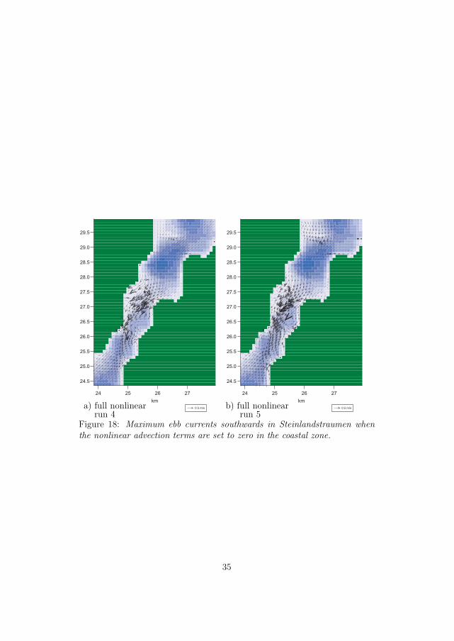
24 25 26 27km

24.5

25.0

25.5

26.0

26.5

27.0

27.5

28.0

28.5

29.0

29.5

0.5 m/s

24 25 26 27km

24.5

25.0

25.5

26.0

26.5

27.0

27.5

28.0

28.5

29.0

29.5

0.5 m/sa) full nonlinear b) full nonlinearrun 4 run 5

Figure 18: Maximum ebb currents southwards in Steinlandstraumen whenthe nonlinear advection terms are set to zero in the coastal zone.

35

Paper 2

Modelling of tides and storm surgesin the Tjeldsund channel

in northern Norway

Paper 3

New current modifiedSchrödinger equations

Dept. of Math. University of Oslo

Mechanics and Applied Mathematics No. 1

ISSN 0809–4403 May 2009

NEW CURRENT MODIFIEDSCHRODINGER EQUATIONS

Karina B. Hjelmervik & Karsten Trulsen

Mechanics Division, Department of Mathematics, University of Oslo, Norway

Abstract

New current modified Schrodinger equations are derived suited tostudy waves on both potential and non–potential inhomogeneous cur-rents. Split–step schemes of first, second, and fourth order are dis-cussed. Different results are presented regarding the current termsand the model setup.

This paper mainly serve as background information for Hjelmervik& Trulsen (2009), but the current modified Schrodinger equations andmodel setup presented here are expected to have an even larger rangeof application possibilities.

1 Introduction

Studies of nonlinear wave–current interactions are of academic interest andimportant in order to reduce safety hazards in ocean currents.

Even linear interaction of waves and currents is still an active field ofresearch. It is well known that linear refraction due to currents can provokelarge waves. Waves encountering an opposing current may obtain reducedwave length and increased wave height and steepness. When waves encounteran opposing current jet, focusing can further enhance the wave intensity nearthe centre of the jet. Linear refraction of waves by currents is known to causenavigational problems, e.g. in the Agulhas current, river estuaries, rip cur-rents, entrances in fjords during outgoing tides, and in tidal flows in thecoastal zone, (Longuet-Higgins & Stewart, 1961; Peregrine, 1976; Gonzalez,1984; Jonsson, 1990; Lavrenov, 1998; Bottin & Thompson, 2002; Mori, Liu& Yasuda, 2002; MacIver, Simons & Thomas, 2006; MacMahan, Thornton& Reniers, 2006). When the steepness thus increases, enhanced nonlinearmodulations is anticipated (Stocker & Peregrine, 1999; Lavrenov & Porubov,

1

2006). However, it is not well known how the enhanced effect of nonlinearitymodify the wave height. Our goal is to investigate how current and nonlin-earity modifies the wave heights for waves propagating on inhomogeneousstationary currents. In this paper we will derive equations and construct anumerical setup for this purpose. We will also study some results regardingthe model setup, the current terms, and different current configurations.

Several different equations are used to study wave–current interactions.Our need to resolve wave phases on non–potential currents restricts us fromemploying several obvious candidates. White (1999) allowed a prescribedcurrent with vorticity, and derived a wave action equation which is a phaseaveraged model. Ray theory (White & Fornberg, 1998) is used for track-ing wave packets. Peregrine & Smith (1979) derived a nonlinear Schrodingerequation useful for caustics where ray theory breaks down. Schrodinger equa-tions have bandwidth constraints which may be problematic. The Zakharov(1968) equation does not have bandwidth constraints, but makes it hard toinclude a prescribed current, and is limited to potential flows.

Here we derive a current modified cubic Schrodinger equation suited forwaves on prescribed, stationary collinear currents. Some related models havealready been published. Stewartson (1977) considered the effects of slowlyvarying depth and current, and derived a cubic Schrodinger equation lim-iting to potential theory. Turpin, Benmoussa & Mei (1983) considered theeffects of slowly varying depth and current, and derived a cubic Schrodingerequation limiting to one horizontal dimension. Gerber (1987) used the vari-ational principle to derive a cubic Schrodinger equation for a non–uniformmedium, limiting to potential theory in one horizontal dimension. Stocker& Peregrine (1999) extended the modified nonlinear Schrodinger equation ofDysthe (1979) to include a slowly varying, periodic current and derived acurrent modified Schrodinger equation. As an application example of theirtheory, they studied the effect on a wave field from a potential surface currentinduced by an internal wave. Their dominant current term, UB, is of cubicorder. We want to study stronger currents. Our equation will be taken upto cubic nonlinearity, and will include waves and currents in two horizontaldimensions allowing horizontal shear.

Several methods may be used to derive nonlinear Schrodinger equationsfor deep water waves: an averaged Lagrangian method (Yuen & Lake, 1982),a spectral method (Zakharov, 1968), and a multiple scales method (Hasimoto& Ono, 1972; Davey & Stewartson, 1974; Dysthe, 1979; Stocker & Peregrine,1999). We have used a multiple scale expansion similar to Mei (1989).

Several numerical methods may be used to solve nonlinear Schrodingerequations. We employ a split–step method using both Fourier methods andfinite difference methods (Lo & Mei, 1985; Weidman & Herbst, 1986; Stocker

2

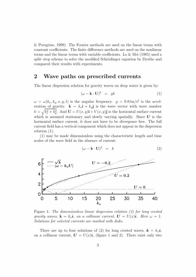
& Peregrine, 1999). The Fourier methods are used on the linear terms withconstant coefficients. The finite difference methods are used on the nonlinearterms and the linear terms with variable coefficients. Lo & Mei (1985) used asplit–step scheme to solve the modified Schrodinger equation by Dysthe andcompared their results with experiments.

2 Wave paths on prescribed currents

The linear dispersion relation for gravity waves on deep water is given by:

(ω − k ·U)2 = gk (1)

ω = ω(kx, ky, x, y, t) is the angular frequency. g = 9.81m/s2 is the accel-eration of gravity. k = kxi + kyj is the wave vector with wave number

k =√

k2x + k2

y. And U = U(x, y)i+ V (x, y)j is the horizontal surface current

which is assumed stationary and slowly varying spatially. Since U is thehorizontal surface current, it does not have to be divergence free. The fullcurrent field has a vertical component which does not appear in the dispersionrelation (1).

(1) may be made dimensionless using the characteristic length and timescales of the wave field in the absence of current:

(ω − k ·U)2 = k (2)

√k|ω− kxU | U = −0.2

U = 0.2

U = 0

kx

Figure 1: The dimensionless linear dispersion relation (2) for long crestedgravity waves, k = kxi, on a collinear current, U = U(x)i. Here ω = 1.Solutions for selected currents are marked with disks.

There are up to four solutions of (2) for long crested waves, k = kxi,on a collinear current, U = U(x)i, (figure 1 and 2). There exist only two

3

ωU

kx/ω2

Figure 2: The linear dis-persion relation (2) forlong crested gravity waves,k = kxi, on a collinearcurrent, U = U(x)i.Both coordinate axes areasymptotes for all curves.ω2 = ±kx when U = 0. Alocal minimum is found in(kx/ω

2, ωU) = (4,−0.25).

solutions when U = 0 or |U | > 14ω

, three solutions when |U | = 14ω

, and foursolutions when |U | < 1

4ω.

Without any current the solutions are ω = ±√k, depending on the di-rection of the waves. If the waves encounter a co–current (kxU > 0), thewavelength increases. If the waves encounter a counter current (kxU < 0),the wavelength decreases. In both cases the phase velocity of the waves isstronger than the group velocity of the waves.

When U = − 14ω

kx

k, the group velocity of the waves has the same strength

as the velocity of the counter current. If the counter current increases fur-ther in strength, there does not exist any solution of the dispersion relationbecause the energy of the waves cannot propagate on such strong countercurrents. If the counter current decreases in strength, the wave train maysplit in two parts with decreasing and increasing wave number respectively.With decreasing wave number the phase velocity of the waves is strongerthan the group velocity of the waves, and as the strength of the counter cur-rent approaches zero, the wave number approaches ω2. With increasing wavenumber the group velocity follows the counter current. As the strength ofthe counter current approaches zero, the wave number approaches infinity.

On a co–current there exist solutions with high wave numbers whichincrease when the strength of the co–current decrease. The group velocityis larger than the phase velocity. This situation cannot be provoked by thecurrent, but if provoked it can exist on a current. When the wave numberexceeds a certain threshold, the capillary waves are more dominant than thegravity waves, see Trulsen & Mei (1993)

4

2.1 Wave path equations

The wave paths are tangential with the group velocity, cg, while the rays aretangential with the wave number vector, k. Since the dispersion relation (2)is not isotropic, the wave paths and the rays do not coincide. The wave pathequations may be written by:

dω

dt=

∂ω

∂t= 0 (3)

dk

dt= −∂ω

∂x= −kx

(∂U

∂xi +

∂U

∂yj

)(4)

dx

dt=

∂ω

∂k= U± 1

2√

k

k

k(5)

Here the x-axis is aligned along the current so that U = U(x, y)i.According to (3) the angular frequency, ω, is constant for each wave path.

Suppose that U = U0 and k = (kx0, ky0) at x = x0. The conserved frequencywill then be:

ω = kx0U0 ±(√

k2x0 + k2

y0

)1/2

(6)

The wave paths are longitudinally reflected when U ± 12√

k

kx

k= 0 and

transversally reflected when ky = 0 according to (5). Suppose that U = URl

when the wave paths are longitudinally reflected, and U = URt when thewave paths are transversally reflected. If ky0 = 0, URl and URt are given by:

URl = − 1

4ω(7)

URt = U0 (8)

The stopping velocity in (7) is in agreement with Peregrine (1976), White &Fornberg (1998), and others.

Following Mei (1989) it can be shown that B satisfies the following con-servation law:

∂

∂t

(B2

σ

)+∇h ·

(cg

B2

σ

)= 0 (9)

B is the amplitude of the waves. σ and cg are given by:

σ = ω −U · kcg = U± 1

2√

k

k

k

5

0 10 20 30 40 50 60−10

−5

0

5

10

0 10 20 30 40 50 601

1.05

1.1

1.15

x

x

y|k|

0 10 20 30 40 50 601

1.05

1.1

1.15

1.2

1.25

|B|

x(a) U0 = 0.1

0 10 20 30 40 50 60−10

−5

0

5

10

0 10 20 30 40 50 601

1.1

1.2

1.3

1.4

1.5

x

x

0 10 20 30 40 50 601

1.2

1.4

1.6

1.8

x(b) U0 = 0.3

0 10 20 30 40 50 60−10

−5

0

5

10

0 10 20 30 40 50 601

1.05

1.1

1.15

1.2

x

x

y|k|

0 10 20 30 40 50 601

1.1

1.2

1.3

1.4

|B|

x(c) U0 = −0.1

0 10 20 30 40 50 60−10

−5

0

5

10

0 10 20 30 40 50 601

1.1

1.2

1.3

1.4

1.5

1.6

x

x

0 10 20 30 40 50 60

2

4

6

8

10

x(d) U0 = −0.3

Figure 3: Wave paths with corresponding wave number, |k|, and amplitude,|B|, as a function of x according to (3)–(5) and (9). The short lines acrossthe wave paths are normal to the wave vector k. Here ω = 1.

6

(9) may also be written on the same form as the wave path equations, inorder to calculate the amplitude while tracing a path:

d

dt

(B2

σ

)=

∂

∂t

(B2

σ

)+ cg · ∇h

(cg

B2

σ

)= −

(B2

σ

)∇ · cg (10)

2.1.1 An example

Suppose that the waves ride a collinear current jet where U = U(y)i:

U(y) = U0 cos2(

πy

Y

)(11)

The rays diverge on co–currents (figure 3a–b) and converge on countercurrents (figure 3c–d). The rays are transversally reflected at the same veloc-ity as the initial velocity in agreement with (8). Since the dispersion relation(2) is not isotropic, the wave vector, k, is not tangential with the wave pathsexcept when the wave vector is parallel to the current, U .

On co–current jets the amplitude and wave number increase towards thechannel walls and decrease towards the centre of the jet. On counter currentjets the amplitude and wave number increase towards the centre of the jet.When the counter current is stronger than the stopping velocity, (7), the raysare reflected longitudinally (figure 3d).

2.2 Exact dispersion for constant current

Suppose that only the positive root is applied in (2):

ω = kxU + kyV +(k2

x + k2y

) 14 (12)

Let ω = 1 + �ω and k = (kx, ky) = (1 + �kx,�ky) where �ω is themodulation frequency and (�kx,�ky) is the modulation wave vector:

1 +�ω = (1 +�kx)U +�kyV +(1 + 2�kx + (�kx)

2 + (�ky)2) 1

4 (13)

Taylor expansion of the last term gives:

�ω − U −�kxU −�kyV − 1

2�kx +

1

8(�kx)

2 − 1

4(�ky)

2

− 1

16(�kx)

3 +3

8�kx(�ky)

2 = O((�k)4

)(14)

7

Following the method of Yuen & Lake (1982) and Trulsen et al. (2000), (14)may then be transformed using the following direct correspondences:

�ω → i∂

∂t, �kx → −i

∂

∂x, �ky → −i

∂

∂y(15)

For a linear, homogeneous wave system of uniform properties these corre-spondences can be made rigorous. When including inhomogeneous currents,the two last relationships in (15) are not accurate unless the ∇U–terms canbe neglected (Stocker & Peregrine, 1999).

Suppose that the current is slowly varying so that the waves do not feelthe changes locally. Then the relations in (15) used on (14) give:

i∂

∂t− U + iU

∂

∂x+ iV

∂

∂y+

i

2

∂

∂x− 1

8

∂2

∂x2+

1

4

∂2

∂y2

− i

16

∂3

∂x3+

3i

8

∂3

∂x∂y2= O

((�k)4

)(16)

If multiplied with −iB, the linear terms in a time evolution of a currentmodified Scrodinger equation appear:

∂B

∂t+

1

2

∂B

∂x+ iUB + U

∂B

∂x+ V

∂B

∂y+

i

8

∂2B

∂x2− i

4

∂2B

∂y2

− 1

16

∂3B

∂x3+

3

8

∂3B

∂x∂y2= O

((�k)4

)(17)

In the next section, current modified nonlinear Schrodinger equations willbe derived using multiple scales. These equations will allow inhomogeneouscurrents.

3 Evolution of current modified nonlinear

Schrodinger equations

Assume that the total velocity field, vtot = v + V , is a superposition of thevelocity of a wave field, v = (u, v, w), and a prescribed stationary currentfield, V = (U, V, W ), in a Cartesian coordinate system, (x, y, z). The x–axisis aligned with the principal propagation direction of the waves. The z–axisis vertical with unit vector k pointing upwards. z = 0 corresponds to theundisturbed free water surface. The water is assumed inviscid, incompress-ible, and deep with respect to the characteristic wavelength. The currentfield is assumed unaffected by waves. η and ζ are the surface displacementsassociated with the wave field and the current field respectively.

8

Potential Vorticity Stocker & HjelmervikStewartson

current allowed Peregrine & Trulsen(1977)

(sec. 3.1) (sec. 3.2) (1999) (2009)akc ε ε 0 ε ε

(U, V )kc/ωc ε ε 1 ε2 εWkc/ωc ε5 ε4 ε2 ε2 ε2

Akc ε2 ε2 0 ε2 ε2

1/kcX ε2 ε ε ε ε1/kcY ε2 1 ε ε ε1/ωcT 0 0 ε2 ε 0

Nonlinear yes yes no yes yesHorizontal

2 2 2 2 2dimensionsPotential

yes no yes yes notheory

Table 1: Current modified Schrodinger equations. kc and ωc are the charac-teristic wave number and frequency for the undisturbed wave field, ω2

c = gkc.a and A are the amplitudes associated with the wave field and the surfacecurrent field respectively. (U, V, W ) is the characteristic current with a char-acteristic length scale (X, Y, Z) and time scale T .

The Euler equation for the combined wave and current field can be writtenas:

∂v

∂t+ vtot · ∇vtot = −1

ρ∇ptot − gk (18)

The total pressure, ptot = p+P +ps, is a combination of the dynamic pressuredue to the wave field, p, the dynamic pressure due to the current field, P ,and the static pressure, ps = pa− ρgz, where pa is the atmospheric pressure,ρ is the density, and g is the acceleration of gravity.

The vorticity of the waves, γ =∇× v, obeys the equation:

∂γ

∂t+ vtot · ∇γ − γ · ∇vtot = −v · ∇Γ + Γ · ∇v (19)

If the vorticity of the current, Γ =∇×V , equals zero, (19) is homogeneouswith respect to γ, and if the wave field starts out irrotational, it will remainirrotational. For waves riding a current field with vorticity, vorticity willdevelop in the wave field as well.

Traditional Schrodinger equations are built on potential theory (Davey& Stewartson, 1974; Stewartson, 1977; Dysthe, 1979; Dysthe & Das, 1981;

9

Gerber, 1987; Stocker & Peregrine, 1999; Trulsen et al., 2000). Here we willderive two current modified nonlinear Schrodinger equations. The first isbuilt on potential theory (sec. 3.1), and the second allows horizontal shearand includes all the terms from the first (sec. 3.2). In table 1 the character-istic sizes of these derivations are compared to some of the derivations foundin literature.

Let a, kc and ωc be the characteristic amplitude, wavenumber and angularfrequency of the surface waves. We employ the steepness of the waves as asmall ordering parameter in the following, ε = akc 1, thus kcη = O(ε) andv kc

ωc= O(ε). The horizontal current velocities are assumed just small enough

to avoid collinear reflection of the waves, (U, V ) kc

ωc= O(ε) . The vertical

surface current velocity is assumed negligible, W kc

ωc= O(ε5) when potential

theory is used, and W kc

ωc= O(ε4) when vorticity is allowed. It follows from

the Bernoulli equation that the surface displacement induced by the currentis small, Akc = O(ε2).

3.1 Potential current field

If the current field is a potential field, V = ∇Φ, the velocity of the wavefield can be represented by a potential, v =∇φ, according to (19).

The continuity equation for the wave field, may be written as:

∇2φ = 0 (20)

The waves are assumed on deep water, that is ∇φ → 0 as z → −∞. Thesurface equations for the combined field at the free surface z = η + ζ , can bewritten as:

∂η

∂t+∇(φ + Φ) · ∇(η + ζ) =

∂

∂z(φ + Φ) (21)

∂φ

∂t+

1

2(∇(φ + Φ))2 + g(η + ζ) = 0 (22)

Taylor expansions around z = 0 gives (21–22) on the form:

∂η

∂t+∇φ · ∇(η + ζ) +∇Φ · ∇η + ζ∇ ∂

∂z(φ + Φ) · ∇η + ζ∇∂φ

∂z· ∇ζ

+η∇ ∂

∂z(φ + Φ) · ∇(η + ζ) +

1

2η(η + 2ζ)∇ ∂

∂z(φ + Φ) · ∇(η + ζ)

+1

2ζ2∇ ∂

∂z(φ + Φ) · ∇η +

1

2ζ2∇∂φ

∂z· ∇ζ +

1

6η3∇∂2φ

∂z· ∇η

=∂φ

∂z+ η

∂2

∂z2(φ + Φ) + ζ

∂2φ

∂z2+

1

2η(η + 2ζ)

∂3

∂z3(φ + Φ) +

1

2ζ2∂3φ

∂z3

10

+1

6η3∂4φ

∂z4+ · · · (23)

∂φ

∂t+ (η + ζ)

∂2φ

∂t∂z+

1

2(η + ζ)2 ∂3φ

∂t∂z2+

1

6(η + ζ)3 ∂4φ

∂t∂z3

+1

2∇φ · ∇(φ + 2Φ) + η∇(φ + Φ) · ∇ ∂

∂z(φ + Φ) + ζ∇(φ + Φ) · ∇∂φ

∂z

+ζ∇φ · ∇∂Φ

∂z+

1

2η2

(∇∂φ

∂z

)2

+1

2η2∇φ · ∇∂2φ

∂z2+ gη + · · · = 0 (24)

Let the horizontal length scales, L, of the current be longer than a charac-teristic wavelength so that 1/(kcL) = O(ε2). In accordance with the scalingassumptions, all equations, variables, and sizes in the following are made di-mensionless using the characteristic length and time scales of the wave field,so that kcx → x, εkcx → x, ωct → t, kcη → εη, kcζ → ε2ζ , 1

ωcφ → εφ,

kc

ωc(U, V ) → ε(U, V ), and kc

ωcW → ε5W ,

The wave field is represented by perturbation series for the surface dis-placement, η, and the velocity potential, φ:

η = εη + 12

(B1e

i(x−t) + εB2e2i(x−t) + ε2B3e

3i(x−t) + · · ·+ c.c.)

φ = εφ + 12

(A′1e

i(x−t) + εA′2e2i(x−t) + ε2A′3e

3i(x−t) + · · ·+ c.c.) (25)

η = η(x, y, t) and φ = φ(x, y, z, t) are the mean surface displacement andmean induced velocity potential respectively. Bn = Bn(x, y, t) and A′n =A′n(x, y, z, t) are the n’th harmonics of the surface displacement and the in-duced current potential respectively. The characteristic wavenumber is fixedappropriate for waves undisturbed by current, therefore the entire effect ofrefraction is represented by modulations of B1.

Both the mean functions and the harmonics, are perturbed:

η = η1 + εη2 + · · · , Bn = Bn0 + εBn1 + ε2Bn2 + · · ·φ = φ1 + εφ2 + · · · , A′n = A′n0 + εA′n1 + ε2A′n2 + · · · (26)

3.1.1 Vertical dependence

The n’th harmonic terms of the scaled continuity equation, (20) is given by:

∂2A′n∂z2

− n2A′n + 2εin∂2A′n∂x

+ ε2

(∂2A′n∂x2

+∂2A′n∂y2

)= 0 (27)

where ∂A′n

∂z→ 0 as z → −∞.

11

First order To first order the continuity equation for A′n (27) is:

∂2A′n0

∂z2− n2A′n0 = 0 (28)

which has the solution:

A′n0 = An0(x, y, t)enz (29)

since∂A′

n0

∂z→ 0 as z → −∞.

Second order To second order the continuity equation for A′n (27) is:

∂2A′n1

∂z2− n2A′n1 + 2in

∂A′n0

∂x= 0 (30)

where∂A′

n1

∂z→ 0 as z → −∞.

Using the result from first order (29), gives:

∂2A′n1

∂z2− n2A′n1 + 2in

∂An0

∂xenz = 0 (31)

which has the solution:

A′n1 = An1(x, y, t)enz − i∂An0

∂xzenz (32)

Third order To third order the continuity equation for A′n (27) is:

∂2A′n2

∂z2− n2A′n2 + 2in

∂A′n1

∂x+

∂2A′n0

∂x2+

∂2A′n0

∂y2= 0 (33)

where∂A′

n2

∂z→ 0 as z → −∞.

Using the results from first and second order (29, 32) gives:

∂2A′n2

∂z2− n2A′n2 + 2in

∂An1

∂x+

∂2An0

∂x2(1 + 2nz)enz +

∂2An0

∂y2enz = 0 (34)

which has the solution:

A′n2 = An2(x, y, t)enz − i∂An1

∂xzenz − 1

2n

∂2An0

∂y2zenz − 1

2

∂2An0

∂x2z2enz (35)

12

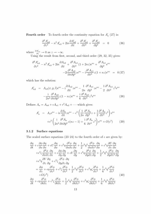
Fourth order To fourth order the continuity equation for A′n (27) is:

∂2A′n3

∂z2− n2A′n3 + 2in

∂A′n2

∂x+

∂2A′n1

∂x2+

∂2A′n1

∂y2= 0 (36)

where∂A′

n3

∂z→ 0 as z → −∞.

Using the result from first, second, and third order (29, 32, 35) gives:

∂2A′n3

∂z2− n2A′n3 + 2in

∂An2

∂x+

∂2An1

∂x2(1 + 2nz)enz +

∂2An1

∂y2enz

−2i∂3An0

∂x∂y2zenz − i

∂3An1

∂x3z(1 + nz)enz = 0 (37)

which has the solution:

A′n3 = An3(x, y, t)enz − i∂An2

∂xzenz − 1

2n

∂2An1

∂y2zenz − 1

2

∂2An1

∂x2z2enz

− i

2n2

∂3An0

∂x∂y2z(1− nz)enz +

i

6

∂3An0

∂x3z3enz (38)

Defines An = An0 + εAn1 + ε2An2 + · · · which gives:

A′n = Anenz − iε∂An

∂xzenz − ε2

(1

2n

∂2An

∂y2z +

1

2

∂2An

∂x2z2

)enz

+ε3

(i

2n2

∂3An

∂x∂y2z(nz − 1) +

i

6

∂3An

∂x3z3

)enz + O(ε4) (39)

3.1.2 Surface equations

The scaled surface equations (23–24) to the fourth order of ε are given by:

∂η

∂t+ ε

∂φ

∂x

∂η

∂x+ εU

∂η

∂x+ ε2η

∂2φ

∂x∂z

∂η

∂x+

1

2ε3η2 ∂3φ

∂x∂z2

∂η

∂x+ ε3η

∂U

∂z

∂η

∂x

+ε3ζ∂2φ

∂x∂z

∂η

∂x+ ε

∂φ

∂y

∂η

∂y+ εV

∂η

∂y+ ε2η

∂2φ

∂y∂z

∂η

∂y+

1

2ε3η2 ∂3φ

∂y∂z2

∂η

∂y

+ε3η∂V

∂z

∂η

∂y+ ε3ζ

∂2φ

∂y∂z

∂η

∂y

=∂φ

∂z+ εη

∂2φ

∂z2+ ε2ζ

∂2φ

∂z2+

1

2ε2η2∂3φ

∂z3+ ε3ηζ

∂3φ

∂z3+

1

6ε3η3∂4φ

∂z4

+O(ε4) (40)

∂φ

∂t+ εη

∂2φ

∂t∂z+ ε2ζ

∂2φ

∂t∂z+

1

2ε2η2 ∂3φ

∂t∂z2+ ε3ηζ

∂3φ

∂t∂z2+

1

6ε3η3 ∂4φ

∂t∂z3

13

+1

2ε

(∂φ

∂x

)2

+ εU∂φ

∂x+ ε2η

∂φ

∂x

∂2φ

∂x∂z+ ε2ηU

∂2φ

∂x∂z+

1

2ε3η2

(∂2φ

∂x∂z

)2

+1

2ε3η2∂φ

∂x

∂3φ

∂x∂z2+

1

2ε3η2U

∂3φ

∂x∂z2+ ε3η

∂φ

∂x

∂U

∂z+ ε3ζ

∂φ

∂x

∂2φ

∂x∂z

+ε3ζU∂2φ

∂x∂z+ ε3ηU

∂U

∂z+

1

2ε

(∂φ

∂y

)2

+ εV∂φ

∂y+ ε2η

∂φ

∂y

∂2φ

∂y∂z

+ε2ηV∂2φ

∂y∂z+

1

2ε3η2

(∂2φ

∂y∂z

)2

+1

2ε3η2∂φ

∂y

∂3φ

∂y∂z2+

1

2ε3η2V

∂3φ

∂y∂z2

+ε3η∂φ

∂y

∂V

∂z+ ε3ζ

∂φ

∂y

∂2φ

∂y∂z+ ε3ζV

∂2φ

∂y∂z+ ε3ηV

∂V

∂z+

1

2ε

(∂φ

∂z

)2

+ε2η∂φ

∂z

∂2φ

∂z2+ ε3ζ

∂φ

∂z

∂2φ

∂z2+

1

2ε3η2

(∂2φ

∂z2

)2

+1

2ε3η2∂φ

∂z

∂3φ

∂z3+ η

= O(ε4) (41)

First order To first order of ε the surface equations (40–41) give:

B10 = iA10 (42)

Second order The zeroth harmonic terms of second order of ε in the dy-namic surface equation (41) are:

i

4B10A

∗10 −

i

4A10B

∗10 +

1

2|A10|2 + η1 = 0 (43)

Using the results from first order (42) gives:

η1 = 0 (44)

The first harmonic terms of second order of ε in the surface equations(40–41) are:

− i

2B11 +

1

2

∂B10

∂t+

i

2B10U =

1

2A11 − i

2

∂A10

∂x(45)

− i

2A11 +

1

2

∂A10

∂t+

i

2A10U +

1

2B11 = 0 (46)

Using the result from first order (42) gives the Schrodinger equation to linearorder:

∂A10

∂x+ 2

∂A10

∂t+ 2iUA10 = 0 (47)

14

and

B11 = iA11 − ∂A10

∂t− iUA10 (48)

The second harmonic terms to second order of ε of the surface equations(40–41) are:

−iB20 − 1

2A10B10 = A20 (49)

−iA20 − i

4A10B10 +

1

2B20 = 0 (50)

Using the result from first order (42) gives:

A20 = 0 (51)

B20 = −1

2A2

10 (52)

Third order The zeroth harmonic terms to third order of ε in the surfaceequations (40–41) are:

∂η1

∂t+

i

4A10

∂B∗10

∂x− i

4B10

∂A∗10∂x

+i

4

∂A10

∂xB∗

10 −i

4

∂B10

∂xA∗10 =

∂φ1

∂z(53)

∂φ1

∂t+

1

4B10

∂A∗10∂t

+i

4B10A

∗11 −

1

4B10

∂A∗10∂x

+1

4

∂A10

∂tB∗

10 −i

4A11B

∗10

−1

4

∂A10

∂xB∗

10 +i

4B11A

∗10 −

i

4A10B

∗11 +

1

2A11A

∗10 −

i

2

∂A10

∂xA∗10

+1

2A10A

∗11 +

i

2A10

∂A∗10∂x

− i

4UB10A

∗10 +

i

4UA10B

∗10 + η2 = 0 (54)

Using the results from first and second order (42, 44, 48) gives:

∂φ1

∂z= −∂|A10|2

∂t(55)

η2 = −∂φ1

∂t(56)

The first harmonic terms of third order of ε in the surface equations (40–41) are:

− i

2B12 +

1

2

∂B11

∂t− 1

2A20B

∗10 +

1

4B20A

∗10 +

i

2UB11

+1

2U

∂B10

∂x+

1

2V

∂B10

∂y− 1

8|B10|2A10 +

1

16B2

10A∗10

15

=1

2A12 − i

2

∂A11

∂x− 1

4

∂2A10

∂y2+

1

2η1A10 +

1

2ζA10 (57)

− i

2A12 +

1

2

∂A11

∂t− i

2η1A10 +

i

4B20A

∗10 − iA20B

∗10 −

i

2ζA10

+i

16B2

10A∗10 −

i

8|B10|2A10 + A20A

∗10 +

i

2UA11

+1

2U

∂A10

∂x+

1

2V

∂A10

∂y+

1

2|A10|2B10 +

1

2B12 = 0 (58)

Using the results from first and second order (42, 44, 47–48, 51–52) gives thecurrent modified cubic nonlinear Schrodinger equation:

∂A11

∂x+ 2

∂A11

∂t+ 2iUA11 + i

∂2A10

∂t2− 6U

∂A10

∂t

+i|A10|2A10 − 5iU2A10 + 2V∂A10

∂y− i

2

∂2A10

∂y2= 0 (59)

and

B12 = iA12 − ∂A11

∂t+ iζA10 − 3i

8|A10|2A10 − iUA11

+2U∂A10

∂t+ 2iU2A10 − V

∂A10

∂y(60)

The second harmonic terms of third order of ε in the surface equations(40–41) are:

−iB21 +1

2

∂B20

∂t− 1

2A10B11 +

i

4A10

∂B10

∂x− 1

2B10A11 +

3i

4

∂A10

∂xB10

+iUB20 = A21 − i

2

∂A20

∂x(61)

−iA21 +1

2

∂A20

∂t− i

4B10A11 − 1

4B10

∂A10

∂x+

1

4B10

∂A10

∂t− i

4A10B11

+iUA20 +i

4UA10B10 +

1

2B21 = 0 (62)

Using the results from first and second order (42, 47–48, 51–52) gives:

A21 = 0 (63)

B21 = −2iA10∂A10

∂t− A10A11 + 2UA2

10 (64)

The third harmonic terms of third order of ε in the surface equations(40–41) are:

−3i

2B30 − 3

4A10B20 − 3

2A20B10 − 3

16B2

10A10 =3

2A30 (65)

−3i

2A30 − iB10A20 − i

4B20A10 − i

16B2

10A10 +1

2B30 = 0 (66)

16

Using the results from first and second order (42, 51–52) gives:

A30 = 0 (67)

B30 = −3i

8A3

10 (68)

Fourth order The first harmonic terms of fourth order of ε in the surfaceequations (40–41) are:

− i

2B13 +

1

2

∂B12

∂t+

i

2

∂φ1

∂xB10 +

i

2

∂η1

∂xA10 + iη1

∂A10

∂x− 1

2η1A11 − 1

2η2A10

−1

2A20B

∗11 −

1

2A21B

∗10 +

1

4B20A

∗11 +

1

4B21A

∗10 −

1

8A10B11B

∗10

−1

8A10B10B

∗11 +

1

8B10B11A

∗10 +

1

16B2

10A∗11 −

1

8|B10|2A11

+i

2A20

∂B∗10

∂x+

i

8A10B10

∂B∗10

∂x+

i

16B2

10

∂A∗10∂x

+3i

8|B10|2∂A10

∂x

+3i

4

∂A20

∂xB∗

10 −i

4

∂B20

∂xA∗10 +

i

8A10

∂B10

∂xB∗

10 −i

8B10

∂B10

∂xA∗10

+i

2UB12 +

1

2U

∂B11

∂x+

1

2V

∂B11

∂y− 1

2ζA11 + iζ

∂A10

∂x

=1

2A13 − i

2

∂A12

∂x− 1

4

∂2A11

∂y2− i

4

∂3A10

∂x∂y2(69)

− i

2A13 +

1

2B13 +

1

2

∂A12

∂t+

i

2

∂φ1

∂xA10 +

1

2

∂φ1

∂zA10 − i

2η1A11 − 1

2η1

∂A10

∂x

+1

2η1

∂A10

∂t− i

2η2A10 − iA20B

∗11 + 2A20A

∗11 + 2A21A

∗10 − iA21B

∗10

+i

4B20A

∗11 +

i

4B21A

∗10 +

1

2A10B11A

∗10 −

i

8A10B11B

∗10

+1

2A10B10A

∗11 −

i

8A10B10B

∗11 +

1

2A11B10A

∗10 −

i

8B10A11B

∗10

+i

8B10B11A

∗10 +

i

16B2

10A∗11 + 2iA20

∂A∗10∂x

− 1

4B20

∂A∗10∂x

+1

4B20

∂A∗10∂t

+3i

4A10B10

∂A∗10∂x

− 1

8B2

10

∂A∗10∂x

+1

16B2

10

∂A∗10∂t

− i∂A20

∂xA∗10

−1

2

∂A20

∂xB∗

10 +1

2

∂A20

∂tB∗

10 −3i

4B10

∂A10

∂xA∗10 −

1

4B10

∂A10

∂xB∗

10

+1

8B10

∂A10

∂tB∗

10 +i

2UA12 + iUA20B

∗10 −

i

4UB20A

∗10 −

i

16UB2

10A∗10

+i

8U |B10|2A10 +

1

2U

∂A11

∂x+

1

2V

∂A11

∂y+

1

2U

∂U

∂zB10 +

1

2V

∂V

∂zB10

17

− i

2ζA11 − 1

2ζ∂A10

∂x+

1

2ζ∂A10

∂t+

i

2ζUA10

= 0 (70)

Using the results from first, second and third order (42, 44, 47–48, 51–52,55–56, 59–60, 63–64, 67–68) gives the current modified nonlinear Schrodingerequation built on potential theory to Dysthe level, MNLSC:

∂A12

∂x+ 2

∂A12

∂t+ i

∂2A11

∂t2 + 2i

∂φ1

∂xA10 − i

2

∂2A11

∂y2− ∂3A10

∂t∂y2

−8A10∂A10

∂tA∗10 + iA2

10A∗11 + 2iA10A11A

∗10 + 2iUA12 − 6U

∂A11

∂t

−6iU∂2A10

∂t2 − 10iUA2

10A∗10 + 2V

∂A11

∂y+ 2iV

∂2A10

∂t∂y− 5iU2A11

+20U2 ∂A10

∂t+ iU

∂U

∂zA10 − 6UV

∂A10

∂y+ iV

∂V

∂zA10 + 14iU3A10

= 0 (71)

3.1.3 Summary

In the following A = A1, B = B1, and (x, y, t) = (x, y, t) to simplify thenotation.

Space evolution of A The space evolution of the MNLSC equation (71)expressed by modulation of A is:

∂A

∂x+ 2

∂A

∂t+ 2iUA

+i∂2A

∂t2− i

2

∂2A

∂y2+ iA|A|2 − 6U

∂A

∂t− 5iU2A + 2V

∂A

∂y

+2i∂φ

∂xA− ∂3A

∂t∂y2− 8|A|2∂A

∂t− 6iU

∂2A

∂t2− 10iUA|A|2 + 2iV

∂2A

∂t∂y

+20U2 ∂A

∂t+ iU

∂U

∂zA− 6UV

∂A

∂y+ iV

∂V

∂zA + 14iU3A = 0 (72)

and

∂φ

∂z= −∂|A|2

∂twhen z = 0 (73)

4∂2φ

∂t2+

∂2φ

∂y2+

∂2φ

∂z2= 0 when z < 0 (74)

∂φ

∂z= 0 when z → −∞ (75)

18

with the following reconstruction formulas:

η = −∂φ

∂tA2, A3 = 0

B = iA− ∂A

∂t− iUA + iζA− 3i

8A|A|2 + 2U

∂A

∂t+ 2iU2A− V

∂A

∂y

B2 = −1

2A2 − 2iA

∂A

∂t+ 2UA2

B3 = −3i

8A3

Space evolution of B The space evolution of the MNLSC equation (71)expressed by modulation of B is:

∂B

∂x+ 2

∂B

∂t+ 2iUB

+i∂2B

∂t2− i

2

∂2B

∂y2+ iB|B|2 − 6U

∂B

∂t− 5iU2B + 2V

∂B

∂y− 4i

∂φ1

∂tB

− ∂3B

∂t∂y2− 8|B|2∂B

∂t− 2B2∂B∗

∂t− 6iU

∂2B

∂t2− 8iU |B|2B + 2iV

∂2B

∂t∂y

+20U2 ∂B

∂t+ iU

∂U

∂zB − 6UV

∂B

∂y+ iV

∂V

∂zB + 14iU3B = 0 (76)

and

∂φ

∂z= −∂|B|2

∂twhen z = 0 (77)

∂2φ

∂x2+

∂2φ

∂y2+

∂2φ

∂z2= 0 when z < 0 (78)

∂φ

∂z= 0 when z → −∞ (79)

with the following reconstruction formulas:

η = −∂φ

∂t

A = −iB − ∂B

∂t− iUB + i

∂2B

∂t2+ iζB − 3i

8|B|2B + iU2B − V

∂B

∂yA2, A3 = 0

B2 =1

2B2 + iB

∂B

∂t− UB2

B3 =3

8B3

19

Time evolution of A The time evolution of the MNLSC equation (71)expressed by modulation of A is:

∂A

∂t+

1

2

∂A

∂x+ iUA

+i

8

∂2A

∂x2− i

4

∂2A

∂y2+

i

2A|A|2 + U

∂A

∂x+ V

∂A

∂y

+i∂φ

∂xA− 1

16

∂3A

∂x3+

3

8

∂3A

∂x∂y2+

3

2|A|2∂A

∂x− 1

4A2∂A∗

∂x

+i

2U

∂U

∂zA +

i

2V

∂V

∂zA = 0 (80)

and

∂φ

∂z=

1

2

∂|A|2∂x

when z = 0 (81)

∂2φ

∂x2+

∂2φ

∂y2+

∂2φ

∂z2= 0 when z < 0 (82)

∂φ

∂z= 0 when z → −∞ (83)

with the following reconstruction formulas:

η =1

2

∂φ

∂xA2, A3 = 0

B = iA +1

2

∂A

∂x+ iζA +

i

8A|A|2 +

i

8

∂2A

∂x2− i

4

∂2A

∂y2

B2 = −1

2A2 + iA

∂A

∂x

B3 = −3i

8A3

Time evolution of B The time evolution of the MNLSC equation (71)expressed by modulation of B is:

∂B

∂t+

1

2

∂B

∂x+ iUB

+i

8

∂2B

∂x2− i

4

∂2B

∂y2+

i

2|B|2B + U

∂B

∂x+ V

∂B

∂y

− 1

16

∂3B

∂x3+

3

8

∂3B

∂x∂y2+

3

2B

∂B

∂xB∗ +

1

4B2∂B∗

∂x+ i

∂φ1

∂xB

+i

2U

∂U

∂zB +

i

2V

∂V

∂zB − i

2U |B|2B = 0 (84)

20

and

∂φ

∂z=

1

2

∂|B|2∂x

when z = 0 (85)

∂2φ

∂x2+

∂2φ

∂y2+

∂2φ

∂z2= 0 when z < 0 (86)

∂φ

∂z= 0 when z → −∞ (87)

with the following reconstruction formulas:

η =1

2

∂φ

∂x

A = −iB +1

2

∂B

∂x+

3i

8

∂2B

∂x2− i

4

∂2B

∂y2+

i

8|B|2B + iζB

A2, A3 = 0

B2 =1

2B2 − i

2B

∂B

∂x

B3 =3

8B3

The CNLS4 equation by Stocker & Peregrine (1999) may be derived from(84) by rescaling.

3.2 Current field with horizontal shear

If the current field is rotational, vorticity develops in the wave field accordingto (19).

The divergence of the Euler equation for the waves (18) is:

∇ · (v ·∇v + v ·∇V + V ·∇v) = −1

ρ∇2p (88)

The surface equations for the combined field at z = η + ζ can be writtenas:

∂η

∂t+ vtot · ∇(η + ζ) = w + W (89)

ptot = p (90)

Taylor expansions around z = 0 gives (89–90) on the form:

∂η

∂t+ vtot · ∇(η + ζ) + (η + ζ)

∂vtot

∂z· ∇(η + ζ) +

1

2(η + ζ)2∂2vtot

∂z2· ∇(η + ζ)

21

= w + W + (η + ζ)∂

∂z(w + W ) +

1

2(η + ζ)

∂2

∂z2(w + W ) + · · · (91)

ptot + (η + ζ)∂ptot

∂z+

1

2(η + ζ)2∂2ptot

∂z2+ · · · = pa (92)

The waves are assumed on deep water, thus v, p→ 0 as z → −∞.Let the current vary more slowly on a length scale along the x–axis, X,

than along the y–axis, Y , so that 1/(kcX) = O(ε) and 1/(kcY ) = O(1). Inaccordance with the scaling assumptions, all equations, variables, and sizesin the following are made dimensionless using the characteristic length andtime scales of the wave field, so that kcx → x, εkcx → x, ωct → t, kcη → εη,kcζ → ε2ζ , kc

ωcv → εv, kc

ωc(U, V ) → ε(U, V ), kc

ωcW → ε4W , kc

ρgp → εp, and

kc

ρgP → ε3P .

Note that in Hjelmervik & Trulsen (2009) the scaling is slightly changed.Since the waves are modulated on a length scale of order ε, the transversallength scale of the current is also assumed of order ε. And the vertical surfacevelocity of the current is assumed of one order lower.

The scaled equation for the divergence of the Euler equation for the waves(88) to the fourth order of ε is:

ε

⎛⎝(∂u

∂x

)2

+

(∂v

∂u

)2

+

(∂w

∂z

)2

+2∂u

∂y

∂v

∂x+2

∂u

∂z

∂w

∂x+2

∂v

∂z

∂w

∂y+2

∂v

∂x

∂U

∂y+2

∂v

∂y

∂V

∂y

⎞⎠+ε2

(2∂u

∂x

∂U

∂x+ 2

∂u

∂y

∂V

∂x

)= −∂2p

∂x2− ∂2p

∂y2− ∂2p

∂z2(93)

The scaled Euler equation for the waves (18) to the fourth order of ε is:

∂u

∂t+ ε

(U

∂u

∂x+ V

∂u

∂y+ v

∂U

∂y+ v · ∇u

)+ ε2u

∂U

∂x= −∂p

∂x(94)

∂v

∂t+ ε

(U

∂v

∂x+ V

∂v

∂y+ v

∂V

∂y+ v · ∇v

)+ ε2u

∂V

∂x= −∂p

∂y(95)

∂w

∂t+ ε

(U

∂w

∂x+ V

∂w

∂y+ v · ∇w

)= −∂p

∂z(96)

The scaled surface equations for the waves (91–92) to the fourth order ofε is:

∂η

∂t+ ε(v + V ) · ∇η + ε2

(v∂ζ

∂y+ η

∂v

∂z· ∇η

)

+ε3

(u

∂ζ

∂x+ η

∂v

∂z

∂ζ

∂y+ ζ

∂v

∂z· ∇η +

1

2η2∂2v

∂z2· ∇η

)

22

= w + εη∂w

∂z+ ε2

(ζ∂w

∂z+

1

2η2∂2w

∂z2

)+ ε3

(ηζ

∂2w

∂z2+

1

6η3∂3w

∂z3

)+ O(ε4)(97)

p− η + εη∂p

∂z+ ε2

(ζ∂p

∂z+

1

2η2 ∂2p

∂z2

)+ ε3

(ηζ

∂2p

∂z2+

1

6η3 ∂3p

∂z3

)= O(ε4) (98)

The wave field is represented by perturbation series for the surface dis-placement, η, the velocity, v, and the dynamic pressure, p:

η = εη + 12

(B1e

i(x−t) + εB2e2i(x−t) + ε2B3e

3i(x−t) + · · ·+ c.c.)

v = εv + 12

(v1ei(x−t) + εv2 e2i(x−t) + ε2v3e3i(x−t) + · · ·+ c.c.

)p = εp + 1

2

(p1 ei(x−t) + εp2 e2i(x−t) + ε2 p3 e3i(x−t) + · · ·+ c.c.

) (99)

We shall assume that the waves are modulated on the slow spatial scales xand y, and a correspondingly slow time scale εt = t. Thus η = η(x, y, t),v = v(x, y, z, t), and p = p(x, y, z, t) are the mean surface displacement,mean induced velocity, and mean dynamic pressure respectively, while Bn =Bn(x, y, t), vn = vn(x, y, z, t), and pn = pn(x, y, z, t) are the n’th harmonicsof the surface displacement, induced current, and dynamic pressure respec-tively. The characteristic wavenumber is fixed appropriate for waves undis-turbed by current, therefore the entire effect of refraction is represented bythe modulation of B1.

Both the mean functions and the harmonics, are perturbed:

η = η1 + εη2 + · · · , Bn = Bn0 + εBn1 + ε2Bn2 + · · ·v = v1 + εv2 + · · · , vn = vn0 + εvn1 + ε2vn2 + · · ·p = p1 + εp2 + · · · , pn = pn0 + εpn1 + ε2 pn2 + · · ·

(100)

3.2.1 First order terms

First harmonic The first harmonic terms of first order of ε for the diver-gence of the Euler equation (93) are:

p10 − ∂2p10

∂z2= 0 (101)

which has the general solution:

p10 = A10(x, y, t)ez (102)

The first harmonic terms of first order of ε in the surface equations (97–98)give:

A10 = B10 (103)

23

The first harmonic terms of first order of ε in the Euler equation (94–96)then give respectively:

u10 = B10ez (104)

v10 = 0 (105)

w10 = −iB10ez (106)

3.2.2 Second order terms

Zeroth harmonic The zeroth harmonic terms of second order of ε for thez–component of the Euler equation (96) are:

i

4u10w

∗10 +

i

4u∗10w10 +

1

4w10

∂w∗10∂z

+1

4w∗10

∂w10

∂z= −∂p1

∂z(107)

Using the results from first order (104, 106) gives:

|B10|2e2z = −∂p1

∂z(108)

which has the solution:

p1 = A1(x, y, t)ez − 1

2|B10|2e2z (109)

The zeroth harmonic terms of second order of ε in the dynamic surfaceequation (98) are:

p1

∣∣∣z=0− η1 +

1

4B10

∂p∗10∂z

∣∣∣z=0

+1

4B∗

10

∂p10

∂z

∣∣∣z=0

= 0 (110)

Using the results from first order (102–103) and the solution for p1 (109)gives A1 = η1.

The zeroth harmonic terms of second order of ε in the kinematic surfaceequation (97) are:

− i

4u10

∣∣∣z=0

B∗10 +

i

4u∗10∣∣∣z=0

B10

= w1

∣∣∣z=0

+1

4B10

∂w∗10∂z

∣∣∣z=0

+1

4B∗

10

∂w10

∂z

∣∣∣z=0

(111)

Using the results from first order (104, 106) gives:

w1

∣∣∣z=0

= 0 (112)

Since no surface elevation or induced current is provoked to first order of ε,η1 = u1 = v1 = w1 = 0 without lack of information.

24

First harmonic The first harmonic terms of second order of ε for thedivergence of the Euler equation (93) are:

2iv10∂U

∂y+ 2i

∂p10

∂x= p11 − ∂2p11

∂z2(113)

Using the results from first order (102–103, 105) gives:

2i∂B10

∂xez = p11 − ∂2p11

∂z2(114)

which has the solution:

p11 = A11(x, y, t)ez − i∂B10

∂xzez (115)

The first harmonic terms of second order of ε in the dynamic surfaceequation (98) give:

A11 = B11 (116)

The first harmonic terms of second order of ε in the Euler equation andthe kinematic surface equation (94–97) are respectively:

∂u10

∂t− iu11 + iu10U + v10

∂U

∂y= −∂p10

∂x− ip11 (117)

∂v10

∂t− iv11 + iv10U + v10

∂V

∂y= −∂p10

∂y(118)

∂w10

∂t− iw11 + iw10U = −∂p11

∂z(119)

∂B10

∂t− iB11 + iUB10 = w11

∣∣∣z=0

(120)

Using the results from first order (102–106) and the solution for p11 (115),leads to the current modified Schrodinger equation to linear order:

∂B10

∂x+ 2

∂B10

∂t+ 2iUB10 = 0 (121)

and the following reconstruction formulas:

u11 = B11ez + i

(∂B10

∂t+ iUB10

)(1 + 2z)ez (122)

v11 = −i∂B10

∂yez (123)

w11 = −iB11ez +

(∂B10

∂t+ iUB10

)(1 + 2z)ez (124)

25

Second harmonic The second harmonic terms of second order of ε for thedivergence of the Euler equation (93) are:

−1

2u2

10 +1

2

(∂w10

∂z

)2

+ i∂u10

∂zw10 = 4p20 − ∂2p20

∂z2(125)

Using the results from first order (104, 106) gives:

0 = 4p20 − ∂2p20

∂z2(126)

which has the solution:

p20 = A20e2z (127)

The second harmonic terms of second order of ε in the dynamic surfaceequation (98) are:

p20

∣∣∣z=0−B20 +

1

2B10

∂p10

∂z

∣∣∣z=0

= 0 (128)

Using the results from first order (102–103) and the solution for p20 (127)gives:

A20 = B20 − 1

2B2

10 (129)

The second harmonic terms of second order of ε in the Euler equationand the kinematic surface equation (94–97) are respectively:

−iu20 +i

4u2

10 +1

4w10

∂u10

∂z= −ip20 (130)

−iv20 +i

4u10v10 +

1

4w10

∂v10

∂z= 0 (131)

−iw20 +i

4u10w10 +

1

4w10

∂w10

∂z= −1

2

∂p20

∂z(132)

−iB20 +i

4u10

∣∣∣z=0

B10 =1

2w20

∣∣∣z=0

+1

4B10

∂w10

∂z

∣∣∣z=0

(133)

Using the results from first order (104–106) and the solution for p20 (127–129)gives:

u20 = v20 = w20 = p20 = 0 (134)

B20 =1

2B2

10 (135)

26

3.2.3 Third order terms

First harmonic The first harmonic terms of third order of ε for the diver-gence of the Euler equation (93) are:

u20u∗10 +

1

2

∂w20

∂z

∂w∗10∂z

− i

2

∂u20

∂zw∗10 + i

∂u∗10∂z

w20

+iv11∂U

∂y+

∂v10

∂x

∂U

∂y+

∂v10

∂x

∂V

∂y+ iu10

∂U

∂x

= −1

2

∂2p10

∂x2− i

∂p11

∂x+

1

2p12 − 1

2

∂2p10

∂y2− 1

2

∂2p12

∂z2(136)

Using the results from first and second order (102–106, 115–116, 123, 134)gives:

∂2p12

∂z2− p12 = −2i

∂B11

∂xez − ∂2B10

∂x2ez − ∂2B10

∂y2ez

−2∂2B10

∂x2zez − 2iB10

∂U

∂xez − 2

∂B10

∂y

∂U

∂yez (137)

which has the solution:

p12 = A12(x, y, z, t)ez + α(x, y, z, t)zez + β(x, y, t)z2ez (138)

where

α = −i∂B11

∂x− 1

2

∂2B10

∂y2− iB10

∂U

∂x− ∂B10

∂y

∂U

∂y

β = −1

2

∂2B10

∂x2

The first harmonic terms of third order of ε in the dynamic surface equa-tion (98) are:

1

2p12

∣∣∣z=0− 1

2B12 +

1

4B20

∂p∗10∂z

∣∣∣z=0

+1

4B∗

10

∂p20

∂z

∣∣∣z=0

+1

2B10

∂p1

∂z

∣∣∣z=0

+1

2ζ∂p10

∂z

∣∣∣z=0

+1

16B2

10

∂2p∗10∂z2

∣∣∣z=0

+1

8|B10|2 ∂2p10

∂z2

∣∣∣z=0

= 0 (139)

Using the results from the first and second order (102–103, 109, 134–135)and the solution for p12 (138), gives:

A12 = B12 +3

8B2

10B∗10 − B10ζ at z = 0 (140)

27

The first harmonic terms of third order of ε in the Euler equation and thekinematic surface equation (94–97) are respectively:

1

2

∂u11

∂t− i

2u12 +

1

2

∂u10

∂xU +

i

2u11U +

1

2

∂u10

∂yV +

1

2v11

∂U

∂y− i

4u20u

∗10

+i

2u∗10u20 +

1

4w20

∂u∗10∂z

+1

4w∗10

∂u20

∂z+

1

2u10

∂U

∂x

= −1

2

∂p11

∂x− i

2p12 (141)

1

2

∂v11

∂t− i

2v12 +

1

2

∂v10

∂xU +

i

2v11U +

1

2

∂v10

∂yV +

1

2v11

∂V

∂y+

1

2u10

∂V

∂x

− i

4u20v

∗10 +

i

2u∗10v20 +

1

4w20

∂v∗10∂z

+1

4w∗10

∂v20

∂z= −1

2

∂p11

∂y(142)

1

2

∂w11

∂t− i

2w12 +

1

2

∂w10

∂xU +

i

2w11U +

1

2

∂w10

∂yV − i

4u20w

∗10

+i

2u∗10w20 +

1

4w20

∂w∗10∂z

+1

4w∗10

∂w20

∂z= −1

2

∂p12

∂z(143)

1

2

∂B11

∂t− i

2B12 − i

4u20

∣∣∣z=0

B∗10 +

i

2u∗10∣∣∣z=0

B20

+1

2

∂B10

∂xU +

i

2B11U +

1

2

∂B10

∂yV +

1

2v10

∣∣∣z=0

∂ζ

∂y

− i

8|B10|2 ∂u10

∂z

∣∣∣z=0

+i

8B2

10

∂u∗10∂z

∣∣∣z=0

+i

8|B10|2∂u10

∂z

∣∣∣z=0

=1

2w12

∣∣∣z=0

+1

4B20

∂w∗10∂z

∣∣∣z=0

+1

2B∗

10

∂w20

∂z

∣∣∣z=0

+1

2ζ∂w10

∂z

∣∣∣z=0

+1

16B2

10

∂w∗10∂z

∣∣∣z=0

+1

8|B10|2∂2w10

∂z2

∣∣∣z=0

(144)

Combining these equations with the results from first and second order (104–106, 115–116, 122–124, 134–135) and the solution for p12 (138, 140) gives thespace evolution of the current modified cubic Schrodinger equation, NLSC:

0 =∂B11

∂x+ 2

∂B11

∂t+ i

∂2B10

∂t2− i

2

∂2B10

∂y2+ iB2

10B∗10 + 2iB11U

−6∂B10

∂tU − 5iB10U

2 + 2∂B10

∂yV + B10

∂U

∂x− i

∂B10

∂y

∂U

∂y(145)

And the time evolution:

0 =∂B11

∂t+

1

2

∂B11

∂x+

i

8

∂2B10

∂x2− i

4

∂2B10

∂y2+

i

2B2

10B∗10

+iB11U +∂B10

∂xU − ∂B10

∂yV +

1

2B10

∂U

∂x− i

2

∂B10

∂y

∂U

∂y(146)

28

3.2.4 Summary

In the following B = B1 to simplify the notation.

Space evolution The space evolution of the current modified nonlinearSchrodinger equation which allows vorticity to the first order of ε, NLSC is:

∂B

∂x= (L+ C +N )B (147)

L contains the linear terms with constant coefficients. C contains the linearterms with variable coefficients. And N is the nonlinear term:

L = −2∂

∂t− i

∂2

∂t2+

i

2

∂2

∂y2

C = −2iU + 6U∂

∂t+ 5iU2 − 2V

∂

∂y− ∂U

∂x+ i

∂U

∂y

∂

∂y

N = −i|B|2

The vertical current component, W , the vertical derivatives of the current,∂V∂z

, and the surface displacement, ζ , associated with the current, appear tothe next order of the equation.

The reconstruction formulas are:

η, u, v, w = 0

p = −1

2|B|2e2z

B2 =1

2B2

u1 = Bez + i∂B

∂tez −BUez + 2i

∂B

∂tzez − 2BUzez

v1 = −i∂B

∂yez

w1 = −iBez +∂B

∂tez + iBUez + 2

∂B

∂tzez + 2iBUzez

p1 = Bez + 2i∂B

∂tzez − 2BUzez

u2, v2, w2, p2 = 0

Time evolution The time evolution of the current modified nonlinearSchrodinger equation which allows vorticity to the first order of ε, NLSCis:

∂B

∂t= (L+ C +N )B (148)

29

where

L = −1

2

∂

∂x− i

8

∂2

∂x2+

i

4

∂2

∂y2

C = −iU − U∂

∂x+ V

∂

∂y− 1

2

∂U

∂x+

i

2

∂U

∂y

∂

∂y

N = − i

2|B|2

The reconstruction formulas are:

η, u, v, w = 0

p = −1

2|B|2e2z

B2 =1

2B2

u1 = Bez − i

2

∂B

∂xez − i

∂B

∂xzez

v1 = −i∂B

∂yez

w1 = −iBez − 1

2

∂B

∂xez − ∂B

∂xzez

p1 = Bez − i∂B

∂xzez

u2, v2, w2, p2 = 0

4 Numerical implementation

4.1 Numerical scheme

Space evolutions of current modified nonlinear Schrodinger equations, (76)and (147), may be written on the form:

∂B

∂x= (L+ V)B (149)

L = L( ∂∂t

, ∂∂y

) contains the linear terms with constant coefficients. V = N+Ccontains the nonlinear term, N = N (|B|2), and the linear terms with variablecoefficients, C = C(U, V, ∂

∂t, ∂

∂y).

4.1.1 Splitting scheme

The formal solution of (149) is:

B = eF (x,y,t)B0 (150)

30

where B0 = B|x=0 and ∂F (x,y,t)∂x

= L+V. If F = F (x, y, t) is weakly dependingon x, (150) may be approximated by:

B ≈ e(L+V)xB0 (151)

The exponential function may be expanded:

e(L+V)x = 1 + (L+ V)x +1

2(L+ V)2x2 +

1

6(L+ V)3x3 + · · · (152)

In numerical simulations LB and VB may be solved separately. Theaccuracy of the result depends on the splitting scheme. Note that it is notnecessary with a more accurate splitting scheme than the accuracy of theseparate solutions.

LV–split With LV–split, e(L+V)x ≈ eLxeVx which may be expanded to:

eLxeVx = 1 + (L+ V)x +1

2

(L2 + 2LV + V2

)x2 + O(x3) (153)

The accuracy is of first order:

e(L+V)x − eLxeVx =1

2(VL − LV)x2 + O(x3) (154)

Note that VL do not equal LV in all cases. An an appropriate commutatoris defined by:

[V,L] ≡ VL − LV (155)

so that (154) may be written on the form:

e(L+V)x − eLxeVx =1

2[V,L]x2 + O(x3) (156)

VLLV–split With VLLV–split, e(L+V)x ≈ e12VxeLxe

12Vx which may be ex-

panded to:

e12VxeLxe

12Vx = 1 + (L+ V)x +

1

2

(L2 + LV + VL+ V2

)x2

+(

1

6L3 +

1

4L2V +

1

8LV2 +

1

4VL2 +

1

4VLV +

1

8V2L+

1

6V3)x3

+O(x4) (157)

This gives an accuracy of second order if [V,L] �= 0:

e(L+V)x − e12VxeLxe

12Vx =

1

24

(2[L, [V,L]

]+[[V,L],V

])x3 + O(x4) (158)

31

(VLLV)3–split With (VLLV)3–splits, a fourth order scheme from Muslu& Erbay (2004) following McLachlan (1994) is used:

e(L+V)x ≈ φ(αx)φ((1− 2α)x

)φ(αx) (159)

where φ(χ) = e12VχeLχe

12Vχ and α = (2+2

13 +2−

13 )/3. This gives an accuracy

of fourth order.

4.1.2 Fourier transform

Fourier transform is used to solved the linear part of (149) with constantcoefficients:

∂B

∂x= LB (160)

The Fourier transform of (160) with respect to y and t is:

∂B

∂x= LB (161)

where L is a complex polynomial of ky and ω. Note that ∂B∂y

= ikyB and

∂B∂t

= −iωB. The exact solution of (160) is:

B = eLxB0 (162)

where B0 = B|x=0.The Fourier transform with respect to y and t is given by:

Bij =1

MN

M−1∑m=0

N−1∑n=0

Bmnei(Ωjtn−kyiym) (163)

where ym = mΔy, tn = nΔt, kyi = iΔky, and Ωj = jΔω.

4.1.3 Finite Difference

Runge–Kutta schemes are used to solve the nonlinear part and the linearpart with variable coefficients in (149):

∂B

∂x= VB (164)

The Runge–Kutta scheme used ought to be of the same order as the splittingscheme.

32

Alternative: a b α βA 0 1 1/2 1/2B 1/2 1/2 1 1C 2/3 1/3 3/2 3/2D 1/3 2/3 3/4 3/4

Table 2: The four alternative choices for the variables in the second orderRunge–Kutta scheme.

First order A first order Euler scheme is used for the first order splittingscheme:

Bx+�x = Bx +�xVxBx (165)

Second order A second order Runge–Kutta scheme is used for the secondorder splitting scheme:

Bx+�x = Bx +�x(ak1 + bk2) (166)

where

k1 = VxBx

k2 = Vx+αx(Bx + β�xk1)

The four coefficients, a, b, α, and β, have to satisfy the following threeequations:

a + b = 1, αb =1

2, βb =

1

2(167)

The four alternatives in table 2 is studied. Lo & Mei (1985) used alternativeA. Alternative B gives the modified Euler scheme.

Fourth order The most used set of variables on the fourth order Runge–Kutta (Gerald & Wheatley, 1994) is used with the fourth order splittingscheme:

Bx+�x = Bx +1

6�x (k1 + 2k2 + 2k3 + k4) (168)

where

k1 = VxBx

33

k2 = Vx+ 12�x

(Bx +

1

2�xk1

)k3 = Vx+ 1

2�x

(Bx +

1

2�xk2

)k4 = Vx+�x (Bx +�xk3)

4.2 Model setup

The space evolution of the current modified nonlinear cubic Schrodingerequation which allows vorticity, NLSC, (147), is simulated. Test simula-tions are performed in order to study the effect of the different terms (seesection 5.3).

The length of the time series are T = 2000. Using N = 1024 nodes,the time step is Δt = T

N≈ 1.95 and �ω = 2π

T≈ 0.0031. The width

of the simulation area, y = [−20, 20], with 16 nodes, gives �y = 2.5 and�ky ≈ 0.079. Test simulations are performed with different widths (seesection 5.2).

4.2.1 Incoming waves

Unidirectional incoming waves with initial Gaussian spectrum have beenstudied. The Fourier amplitudes at x = 0 are given by:

Bj = ε

√ �ω√2πσω

e− Ω2

j

4σ2ω

+iψj(169)

The frequency is given by ωj = 1 + Ωj . The phases, ψi,j , are statistically in-dependent and uniformly distributed on the interval [0, 2π). We have chosenε = 0.1. σω = 0.1 is the bandwidth in Fourier space.

Test simulations with an incoming Stokes wave are also performed (seesections 5.2 and 5.4).

4.2.2 Current field

The NLSC equation may be used for a large range of prescribed currents.Here we have chosen two types; a surface current jet given by:

U =

⎧⎪⎪⎨⎪⎪⎩0 when x ≤ X and/or |y| ≥ Y

U0 sin2(

π2�X

(x−X))

cos2(

πy2Y

)when x > X and x < X +�X

U0 cos2(

πy2Y

)when x ≥ X +�X

(170)

34

and a transversally uniform current given by:

U =

⎧⎪⎪⎨⎪⎪⎩0 when x ≤ X

U0 sin2(

π2�X

(x−X))

when x > X and x < X +�X

U0 when x ≥ X +�X

(171)

The wave field is allowed about 32 wavelengths, x = [0, X) where X = 200,to develop before the waves encounter a current. Y = 10 is half the width ofthe jet. And�X = 100 is the current build–up length. Test simulations withdifferent build–up lengths and widths of the jet are performed (see sections5.7 and 5.6).

We have studied three current cases: no current, co–current with U0 =0.05, and opposing current with U0 = −0.05 which is not enough to reflect thewaves, but sufficient to study the characteristic features of opposing currents.Test simulations are performed with other current strengths (see section 5.5).

Simulations and observations of tidal currents suggest that establishingcurrent jets are more fanned in than terminating current jets are fanned out(Hjelmervik et al., 2005, 2008). Test simulations show that the current acrossthe jet, V , needed to satisfy the continuity equation, has negligible impacton the results and may thus be set to zero in the NLSC equation (see section5.4). Alternatively, the continuity equation can be satisfied by a verticalcurrent, W , which does not appear within the truncation level of the NLSCequation.

4.3 Numerical order

Here the order of different schemes with and without currents is studied.

4.3.1 Transversally uniform currents

The transversally uniform current is given by (171) with U0 = 0, 0.05, and-0.05. The incoming waves are unidirectional and given by (169). The incom-ing phase is randomised in the same way in all simulations. The distributionsof η and |B| at x = 0 are shown in figure 4.

Time series of the envelope, B, at x = 900 from simulation j is used tocalculate the error:

Ej = |B|j − |B|ref (172)

The results with the smallest step, �x = 0.001, is used as the reference solu-tion. Simulations which broke down earlier than x = 900, are not considered.

35

Figure 4: The distributions of surface elevation, η, (left) and envelope, |B|,(right) at x = 0 compared to a Gaussian and a Rayleigh distribution (smoothline) respectively.

The errors, L1 and L2, are calculated from the following formulas:

L1 = ||Ej ||1 =∫ ∞−∞|Ej|dt (173)

L2 = ||Ej ||2 = 2

√∫ ∞−∞

E 2j dt (174)

The simulations are of the expected order both with and without currents(figure 5). The four alternatives in table 2 give slightly different convergencerate (figure 6a).

4.3.2 Current jets

The current jet is given by (170) with U0 = 0, 0.05, and -0.05. The incomingwaves are unidirectional and given by (169). The incoming phase is ran-domised in the same way in all simulations. The distributions of η and |B|at x = 0 are shown in figure 4.

Time series of the envelope, B, for all values of y at x = 400 from simu-lation j is used to calculate the error:

Ej = |B|j − |B|ref (175)

The results with the smallest step, �x = 0.001, used as a reference solution.Simulations which broke down earlier than x = 400, are not considered.

L1 and L2 are calculated from the following formulas:

L1 = ||Ej||1 =∫ ∞−∞

∫ ∞−∞|Ej|dy dt (176)

L2 = ||Ej||2 = 2

√∫ ∞−∞

∫ ∞−∞

E 2j dy dt (177)

The simulations are of the expected order both with and without currentfor first and second order schemes (figure 7a). The four alternatives in table2 give slightly different convergence rate (figure 6b).

36

Without any current, the simulations are of fourth order when the fourthorder scheme is used (figure 7b). The current depends on x and this isprobably the reason why the simulations with current diverge from fourthorder when the fourth order scheme is used. The function, F = F (x, y, t) in(150) might therefore be better approximated by:

F (x, y, t) = (L+ V)0x +1

2

(∂V∂U

∂U

∂x+

∂V∂V

∂V

∂x

)0

x2 + · · · (178)

New splitting schemes have to be constructed in order to improve the fourthorder scheme.

In the following, the second order scheme with alternative A and anintegrating step of �x = 0.2 is used.

37

10−2 10010−7

10−6

10−5

10−4

10−3

10−2

10−1

100

10

102

U = 0U = 0.05U = −0.05

step, �x

1st order

2nd order

4th order

L1

10−2 10010−7

10−6

10−5

10−4

10−3

10−2

10−1

100

U = 0U = 0.05U = −0.05

step, �x

1st order

2nd order

4th order

L2

100 1010−7

10−6

10−5

10−4

10−3

10−2

10−1

100

cpu−time

U = 0U = 0.05U = −0.05

1st order

L2

2nd order

4th order

Figure 5: The L1 (left) and L2 (middle) errors as a function of integratingstep, �x, and the L2 errors as a function of cpu–time (right) for simulationswith unidirectional incoming waves on transversally uniform currents. Thedotted lines represent 1st, 2nd, and 4th order respectively.

10−2 10−1 100 10

10−5

100

alt. Aalt. Balt. Calt. D

step, �x

L2

(a) no current

10−2 10−1 100 1010−5

100

alt. Aalt. Balt. Calt. D

step, �x

L2

(b) co–current jet

Figure 6: The L2 errors for the four alternative second order schemes. Thedotted lines represent 2nd order.

38

10−2 10010−5

10−4

10−3

10−2

10−1

100

10

102

103

104

U = 0U = 0.05U = −0.05

step, �x

1st order

2nd order

L1

10−2 10010−7

10−6

10−5

10−4

10−3

10−2

10−1

100

101

U = 0U = 0.05U = −0.05

step, �x

1st order

2nd order

L2

101 10 10310−5

10−4

10−3

10−2

10−1

100

101

cpu−time

U = 0U = 0.05U = −0.05

L2

1st order

2nd order

(a) 1st and 2nd order

10−2 10010−6

10−5

10−4

10−3

10−2

10−1

100

10

102

103

U = 0U = 0.05U = −0.05

step, �x

L1

4th order

10−2 10010−7

10−6

10−5

10−4

10−3

10−2

10−1

100

101

U = 0U = 0.05U = −0.05

step, �x

L2

4th order

101 10 10310−5

10−4

10−3

10−2

10−1

100

101

cpu−time

U = 0U = 0.05U = −0.05

L2

(b) 4th order

Figure 7: The L1 (left) and L2 (middle) errors as a function of integratingstep, �x, and the L2 errors as a function of cpu–time (right) for simulationswith unidirectional incoming waves on current jets. The dotted lines represent1st, 2nd, and 4th order respectively.

39

5 Numerical results

A few results from simulations with the space evolution of the NLSC equationwhich allows vorticity, (147), will be presented. More results are publishedin Hjelmervik & Trulsen (2009).

The reconstruction of the surface elevation according to section 3.2, isgiven by:

η =1

2

(Bei(x−t) +

1

2εB2e2i(x−t) + c.c.

)+ O(ε2) (179)

As pointed out by Tayfun (1980) and others the second harmonic termsintroduce a vertical asymmetry to the profile caused by the first harmonicterms. The crest become narrower and sharper and throughs become longerand shallower as illustrated in figure 8. Since both the envelope of the crestand the envelope of the through are displaced upward by the second harmonicterms, the distribution of wave heights remain the same. The mean value ofthe highest third of the wave heights – traditionally used as the significantwave height – also remains the same. The more modern definition of thesignificant wave height – four times the standard deviation of the surfaceelevation – is affected, but the change is negligible.

Figure 8: An illustrative reconstruction of the surface elevation and the corre-sponding envelopes for fixed x or t. The dotted lines represent the first orderreconstruction of (179) with B = 0.5. The solid lines represent the secondorder reconstruction which causes the crests to become narrower and sharperand the throughs to become longer and shallower. The wave heights remainunchanged.

The first order reconstruction of the surface displacement is used to cal-culate both the significant wave height, Hs, and the kurtosis, κ, of the surfacedisplacement:

Hs(x, y) = 4√

η2 = 4

√1

2|B|2 (180)

40

κ(x, y) =η4

η22 =

3

2

|B|4|B|22 (181)

The bar represents combined time and ensemble averaging. The kurtosisequals three when the surface elevation is Gaussian distributed.

When the waves meet an opposing current, the wave height increasesin the centre of the jet, and decreases at the sides of the jet. When thewaves meet an co–current, the wave height decreases in the centre of the jet,and increases at the sides of the jet. The following sections show how thesechanges depend on the number of simulations in an ensemble (sec. 5.1), thewidth of the simulation area (sec. 5.2), the different terms in the NLSCequation (sec. 5.3), the transversal current (sec. 5.4), the current strength(sec. 5.5), the width of the jet (sec: 5.6), and the current build–up length(sec. 5.7).

Figure 9: The significant wave height (upper) and kurtosis (lower) from30 single simulations (dots) and from ensembles consisting of 5 (green), 10(black), 20 (red), and 30 (blue) simulations.

41

5.1 Number of simulations in an ensemble

In order to assure statistical and numerical convergence a sufficient num-ber of simulations should be included. Test simulations are performed withincoming unidirectional waves (169), and opposing current jet (170) withU0 = −0.05.

More simulations are needed in order to calculate the kurtosis than thesignificant wave height (figure 9). If only the significant wave height andsimilar qualities are wanted, 10 simulations are sufficient. In the followingwe have used 30 simulations in each ensemble in order to get a more reliableresult also for properties as the kurtosis.

5.2 Width of the simulation area

Test simulations are performed with different widths of the simulation area.The current jet is kept narrow (|y| < 10). The incoming wave is a Stokeswave. Simulations are performed with both a co–current with U0 = 0.05 andan opposing current jet with U0 = −0.05.

When the waves encounter a co–current jet, the amplitudes decrease inthe centre of the jet and increase at the sides of the jet. The high amplitudescreated at the sides of the jet, propagate away from the jet towards thesimulation borders and seem to be reflected there (figure 10). When thewidth of the simulation area is |y| < 40, the high amplitudes are not reflectedbefore x = 375. The amplitude in the centre of the jet seems to be periodicwith a length that depends on the width of the simulation area.

When the waves encounter an opposing current jet, the amplitudes in-crease in the centre of the jet and decrease at the sides of the jet. Theamplitude of the waves are affected only in a narrow area limited by thecurrent jet (figure 11). The amplitude in the centre of the jet seems to beperiodic with a length that does not depend on the width of the simulationarea as long as the simulation area is wider than the width of the jet.

The fact that the waves converge and diverge when encountering currents,makes it possible to create very beautiful plots of the surface elevation. Heller(2005) published an art plot in an electronic art and animation catalog.

42

x

y

200 250 300 350 400 450 500 550 600

−100

10

x

y

200 250 300 350 400 450 500 550 600

−20

0

20

x

y

200 250 300 350 400 450 500 550 600

−40

−20

0

20

40

x

y

200 250 300 350 400 450 500 550 600

−80

−60

−40

−20

0

20

40

60

80

Figure 10: |B| on a co–current when y < 10 (upper), |y| < 20, |y| < 40, and|y| < 80 (lower). Nonlinear. Red is high values, blue small. The dotted linesmark the region of the jet.

43

x

y

200 250 300 350 400 450 500 550 600

−100

10

x

y

200 250 300 350 400 450 500 550 600

−20

0

20

x

y

200 250 300 350 400 450 500 550 600

−40

−20

0

20

40

x

y

200 250 300 350 400 450 500 550 600

−80

−60

−40

−20

0

20

40

60

80

Figure 11: |B| on a counter current when y < 10 (upper), |y| < 20, |y| < 40,and |y| < 80 (lower). Nonlinear. Red is high values, blue small. The dottedlines mark the region of the jet.

44

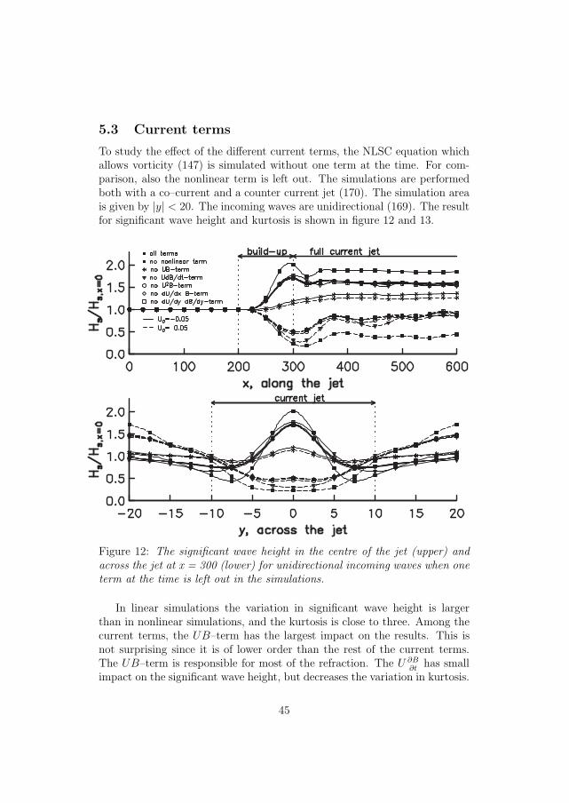
5.3 Current terms

To study the effect of the different current terms, the NLSC equation whichallows vorticity (147) is simulated without one term at the time. For com-parison, also the nonlinear term is left out. The simulations are performedboth with a co–current and a counter current jet (170). The simulation areais given by |y| < 20. The incoming waves are unidirectional (169). The resultfor significant wave height and kurtosis is shown in figure 12 and 13.

Figure 12: The significant wave height in the centre of the jet (upper) andacross the jet at x = 300 (lower) for unidirectional incoming waves when oneterm at the time is left out in the simulations.

In linear simulations the variation in significant wave height is largerthan in nonlinear simulations, and the kurtosis is close to three. Among thecurrent terms, the UB–term has the largest impact on the results. This isnot surprising since it is of lower order than the rest of the current terms.The UB–term is responsible for most of the refraction. The U ∂B

∂thas small

impact on the significant wave height, but decreases the variation in kurtosis.

45

Figure 13: The kurtosis across a co–current (upper) and counter current(lower) jet at x = 300 for unidirectional incoming waves when one term atthe time is left out in the simulations.

Note that the terms that do not appear in the current modified nonlin-ear Schrodinger equation built on potential theory, the ∂U

∂y∂B∂y

–term and the∂U∂x

B–term, have small impact on the results. The U2B–term also has minorimpact. With a stronger current, these terms may have a stronger effect.

In this case, a good approximation for the NLSC equation is the simplifiedNLSC equation given by:

∂B

∂x+ 2

∂B

∂t+ i

∂2B

∂t2− i

2

∂2B

∂y2+ 2iUB − 6U

∂B

∂t+ i|B|2B = 0 (182)

Note that in Hjelmervik & Trulsen (2009) we used a different scaling ofthe modulation of the current normal to the principal propagation directionof the waves. This causes the ∂U

∂y∂B∂y

–term to be left out to the truncationlevel of the NLSC equation.

46

5.4 Transversal current, V

The continuity equation for the current has to be satisfied:

∂U

∂x+

∂V

∂y+

∂W

∂z= 0 (183)

During the build–up of the longitudinal current given by (170) or (171), thefirst term in (183) is not zero. If both the transversal current, V , and thevertical current, W , is set to zero, (183) is therefore not satisfied. Heretwo alternatives for the current jet is discussed. The transversally uniformcurrent is not considered.

x<X X < x < X +�X x > X +�XU=0 U=0 U=0

y>YW=0W=0 W=0

U=0 U=U0 sin2(

π2�X

(x−X))

cos2(

πy2Y

)e−απz U=U0 cos2

(πy2Y

)|y|<Y

W=0W=−U01

2α�Xsin(

π�X

(x−X))

cos2(

πy2Y

)e−απzW=0

U=0 U=0 U=0y<−Y

W=0W=0 W=0

Table 3: A possible current jet when V = 0.

x<X X < x < X +�X x > X +�XU=0 U=0 U=0

y>YV =0 V =−U0

πY4�X

sin(

π�X

(x−X))

V =0

U=0 U=U0 sin2(

π2�X

(x−X))

cos2(

πy2Y

)U=U0 cos2

(πy2Y

)|y|<Y

V =0 V =−U0Y

4�Xsin(

π�X

(x−X)) (

cos(

πyY

)+ πy

Y

)V =0

U=0 U=0 U=0y<−Y

V =0 V =U0πY

4�Xsin(

π�X

(x−X))

V =0

Table 4: A possible current jet when W = 0.

At one extreme, the transversal current is set to zero. A possible currentjet is then given in table 3. The parameter α tells how quickly the currentdecrease towards the bottom. If the scaling in section 3.1 or 3.2 is applied,α has to be less than 0.05. The vertical current first appears in the currentmodified Schrodinger equation to Dysthe level, and is not implemented innumerical models for cubic Schrodinger equations.

At the other extreme, the vertical current is set to zero. A possible currentjet is then given in table 4. A few simulations are performed with the current

47

jet given in table 4. The incoming wave is a Stokes wave. Both linear andnonlinear simulations are performed with both a co–current with U0 = 0.05and an opposing current with U0 = −0.05. The results are compared withresults from simulations with V = 0. The transversal current has little effectin all simulations. The effect on the envelope is shown in figures 14–15.

To assume that both the vertical and the transversal currents equal zero,seems to be a good approximation in this case.

x

y

200 250 300 350 400 450 500 550 600

−40

−20

0

20

40

x

y

200 250 300 350 400 450 500 550 600

−40

−20

0

20

40

Figure 14: |B| on a co–current with V = 0 (upper) and V �= 0 (lower). Highvalues are red, small values are blue.

48

x

y

200 250 300 350 400 450 500 550 600

−40

−20

0

20

40

x

y

200 250 300 350 400 450 500 550 600

−40

−20

0

20

40

Figure 15: |B| on a counter current with V = 0 (upper) and V �= 0 (lower).High values are red, small values are blue.

49

5.5 Current strength

Test simulations are performed with different strengths of the current jet,(170). The simulation area is given by |y| < 20 The incoming waves areunidirectional (169).

The significant wave height in the centre of the jet increases with in-creasing strength of the opposing current jet, and decreases with increasingstrength of the co-current (figure 16). The significant wave height seems tooscillate with a period depending on the strength of the current jet.

Note that in the derivation of the Schrodinger equations, U0 is assumedof order ε. The spectrum is not narrow banded when |U0| = 0.25, and thesimulations seem to break down when |U0| > 0.25. On counter currents thismay be due to longitudinal refraction. When U = U(x)i the dimensionlessstopping velocity is U = −1

4according to (7) and linear ray theory (Peregrine

& Smith, 1979).

Figure 16: The significant wave height of waves in the centre of current jetswith different strengths: |U0| = 0 (square, dotted), 0.01 (square, solid), 0.05(triangle, dotted), 0.10 (triangle, solid), 0.25 (disk, dotted), and 0.50 (disk,solid).

5.6 Width of the jet

Test simulations are performed with different widths, Y , of the current jet(170). The simulation area is given by |y| < 40 The incoming waves areunidirectional (169). Simulations are performed with both a co–current andan opposing current jet.

The significant wave height along the centre of the jet and across the jetchanges more slowly the wider the jet is (figure 17). On an opposing currentjet, the significant wave height does not depend on the width of the jet when

50

the waves are adjusted to the current jet. When the width of the jet equalsthe width of the simulation area, oscillations occur due to channel effects.

Figure 17: The significant wave height in the centre of a co–current and acounter current jet (upper) and across a counter current jet at x=300 (lower)with different widths of the jet.

5.7 Build–up length

Test simulations are performed with different build–up lengths, �X, of thecurrent jet, (170). The simulation area is given by |y| < 40 The incomingwaves are unidirectional (169).

Both the significant wave height and the kurtosis in the centre of thejet change quicker with shorter build–up lengths (figure 18). On opposingcurrent jets the significant wave height seems to oscillate more with shorterbuild–up lengths, but stabilises around the same value after the build–upindependent of the build–up length. The kurtosis decreases more quicklywith shorter build–up lengths of opposing jets. On co–current jets channel

51

effects are more pronounced for shorter build–up lengths due to a strongerdivergence during the build–up. The kurtosis increases quicker and reachesa larger maximum with shorter build–up lengths of the co–current.

Figure 18: The significant wave height (upper) and kurtosis (lower) of wavesin the centre of current jets with different build–up lengths.

52

6 Conclusion

Two new current modified Schrodinger equations have been derived; oneusing potential theory, and one allowing vorticity (NLSC). The splittingschemes are described and the corresponding numerical orders tested. Sincethe current is inhomogeneous, new fourth order splitting schemes should beconstructed.

Monte–Carlo simulations are performed to estimate statistical wave prop-erties. 30 simulations in each ensemble is found to be sufficient to assurestatistical and numerical convergence for higher order properties as the kur-tosis. Different model setups are studied. When waves encounter a countercurrent, the simulation area should be wider than twice the width of the jet.

To study the effect of each current term in the NLSC equation, simulationsare performed without one term at the time. It is found that the currentterm to linear order contains most of the refraction. The nonlinear term haslarger impact than the rest of the current terms. The contribution from thetransversal current required to satisfy the continuity equation for the current,is shown to be negligible for waves on collinear jets.

The statistical wave properties are also used to illustrate different currentjet configurations. If the strength of the counter current jet is increased, thewave height increases and seems to oscillate with a period depending on thestrength of the jet. After the waves are adjusted to a counter current, thesignificant wave height does not seem to depend on neither the width nor thebuild–up length of the jet.

The current modified Schrodinger equation and model setup presentedhere are expected to have a large range of application possibilities. Theoccurrence of freak waves on collinear currents is discussed in Hjelmervik &Trulsen (2009).

Here only collinear currents are studied. The transversal current is as-sumed at the same strength as the longitudinal current in the derivation ofthe current modified nonlinear Schrodinger equation which allows vorticity.Thereby the equation may be used for oblique waves on current jets.

The current modified nonlinear Schrodinger equation for potential cur-rents is derived to Dysthe level. It can easily be implemented in the numericalmodel. And the results are expected to be interesting. Schrodinger equationsto Dysthe level are known to lower the kurtosis.

53

References

Bottin, R. R. Jr. & Thompson, E. F. 2002 Comparisons of physicaland numerical model wave predictions with prototype data at Morro Bayharbor entrance, California. U. S. Army Engineer.

Davey, A. & Stewartson, K. 1974 On three-dimensional packets of sur-face waves. Proc. R. Soc. Lond. A 338, 101–110.

Dysthe, K. B. 1979 Note on the modification to the nonlinear Schrodingerequation for application to deep water waves. Proc. R. Soc. Lond. A 369,105–114.

Dysthe, K. B. & Das, K. P. 1981 Coupling between a surface-wave spec-trum and an internal wave: modulational interaction. J. Fluid Mech., 104,483-503.

Forristall, G. 1978 On the statistical distribution of wave heights in astorm. J. Geophys. Res. 83 8C5), 2353–2358.

Gerald, C. F. & Wheatley, P. O. 1994 Applied Numercial Analysis -Fifth edition. Addison-Wesley Publishing company, Inc.

Gerber, M. 1987 The Benjamin-Feir instability of a deep water Stokeswavepacket in the presence of a non-uniform medium. J. Fluid Mech. 176,311–332.

Gonzalez, F. I. 1984 A case study of wave-current-bathymetry interactionsat the Columbia river entrance. J. Phys. Oceanogr. 14, 1065–1078.

Hasimoto, H. & Ono, H. 1972 Nonlinear modulation of gravity waves.J. Phys. Soc. Japan. 33, 805–811.

Heller, E. 2005 Eric Heller. In ACM SIGGRAPH 2005 Electronic Artand Animation Catalog (Los Angeles, California, August 01 - 04, 2005).SIGGRAPH ’05. ACM, New York, NY, 78-79.

Hjelmervik, K., Ommundsen, A. & Gjevik, B. 2005 Implementationof non-linear advection terms in a high resolution tidal model. Universityof Oslo, preprint.

Hjelmervik, K., Lynge, B. K., Ommundsen, A. & Gjevik, B. 2008Interaction of tides and storm surges in the Tjeldsunet channel in northernNorway. Ocean Dynamics (submitted).

54

Hjelmervik, K. & Trulsen, K 2008 Freak wave statistics on collinearcurrents J. Fluid Mech. (submitted).

Jonsson, I. G. 1990 Wave-current interactions. In The Sea, Ocean Eng. Sci.(ed. by B. Le Mehaute & D. M. Hanes), pp. 65–120, Wiley-Interscience,Hoboken, N. J.

Lavrenov, I. V. 1998 The wave energy concentration at the Agulhas cur-rent off South Africa. Natural Hazards 17, 117–127.

Lavrenov, I. V. & Porubov, A. V. 2006 Three reasons for freak wavegeneration in the non-uniform current. Eur. J. Mech. B/Fluids 25, 574–585.

Lo, E. Y. & Mei, C. C. 1985 A numerical study of water-wave modulationbased on a higher-order nonlinear Schrodinger equation. J. Fluid Mech.150, 395–416.

Longuet-Higgins, M. S. & Stewart, R. W. 1961 The changes in am-plitude of short gravity waves on steady non-uniform currents. J. FluidMech. 10, 529–549.

MacIver R. D., Simons, R. R. & Thomas, G. P. 2006 Gravity wavesinteracting with narrow jet-like current. J. Geophys. Res. 111, C03009.

MacMahan, J. H., Thornton, E. B. & Reniers, A. J. H. M. 2006Rip current review. Coastal Engineering 53, 191–208.

McLachlan, R. 1994 Sympletic integration of Hamiltonian wave equation.Numer. Math. 66 465.

Mei, C. C. 1989 The applied Dynamics of ocean surface waves. World Sci-entific Publishing Co., Singapore., ISBN 9971-50-789-7

Mori, N., Liu, P. C. & Yasuda, T. 2002 Analysis of freak wave mea-surements in the sea of Japan. Ocean Engineering 29, 1399–1414.

Muslu, G. M. & Erbay, H. A. 2004 Higher-order split-step FourierSchemes for the generalized nonlinear Schrodinger equation. Mathemat-ics and Computers in Simulation 67, 581–595.

Peregrine, D. H. 1976 Interaction of water waves and currents. Adv. Appl.Mech. 16, 9–117.

55

Peregrine, D. H. & Smith, R. 1979 Nonlinear effects upon waves nearcaustics. Phil. Trans. R. Soc. Land. A 292, 341–370.

Stewartson, K. 1977 On the resonant interaction between a surface waveand a weak surface current. Mathematika 24, 37–49.

Stocker, J. D. & Peregrine, D. H. 1999 The current-modified nonlinearSchrodinger equation. J. Fluid Mech. 399, 335–353.

Tayfun, M. A. 1980 Narrow-band nonlinear sea waves. J. Geophys. Res.85, 1548–1552.

Trulsen, K., Kliakhandler, I., Dysthe, K. B., & Velarde, M. G.

2000 On weakly nonlinear modulation of waves on deep water. Phys. Fluids12, 2432–2437.

Trulsen, K. & Mei, C. C. 1993 Double reflection of capillary/gravitywavs by a non-uniform current: a boundary–layer theory. J. Fluid Mech.251, 239–271.

Turpin, F-M., Benmoussa, C. & Mei, C. C. 1983 Efects of slowlyvarying depth and current on the evolution of a Stokes wavepacket. J. FluidMech. 132, 1–23.

Weidman, J. A. C. & Herbst, B. M. 1986 Split-step methods for thesolution of the nonlinear Schrodinger equation. SIAM J. Numer. Analy.23, 485–507.

White, B. S. 1999 Wave action on currents with vorticity. J. Fluid Mech.386, 329–344.

White, B. S. & Fornberg, B. 1998 On the chance of freak waves at sea.J. Fluid Mech. 335, 113–138.

Yuen, H. C. & Lake, B. M. 1982 Nonlinear dynamics of deep-watergravity waves. Adv. Appl. Mech. 22, 67–229.

Zakharov, V. E. 1968 Stability of periodic waves of finite amplitude onthe surface of a deep fluid. J. Appl. Mech. Tech. Phys. 9, 86–94.

56

Paper 4

Freak wave statistics on collinear currents

Karina B. Hjelmervik and Karsten Trulsen. Freak wave statistics on collinear currents. Journal of Fluid Mechanics (2009), 637:267-284 Cambridge University Press

Copyright © Cambridge University Press 2009

This is an author produced version of the article. The original publication is available at http://dx.doi.org/10.1017/S0022112009990607

Access to the published version may require journal subscription.

Under consideration for publication in J. Fluid Mech. 1

Freak wave statistics on collinear currents

KARINA B. HJELMERVIKAND KARSTEN TRULSEN

Mechanics Division, Department of Mathematics, University of Oslo, Norway

(Received ?? and in revised form ??)

Linear refraction of waves on inhomogeneous current is known to provoke extremewaves. We investigate the effect of nonlinearity on this phenomenon, with respect tothe variation of significant wave height, kurtosis and occurrence of freak waves. Monte–Carlo simulations are performed employing a modified nonlinear Schrodinger equationthat includes the effects of a prescribed non–potential current. We recommend that freakwaves should be defined by a local criterion according to the wave distribution at eachlocation of constant current, not by a global criterion that is either averaged over, orinsensitive to, inhomogeneities of the current. Nonlinearity can reduce the modulationof significant wave height. Depending on the configuration of current and waves, thekurtosis and probability of freak waves can either grow or decrease when the wave heightincreases due to linear refraction. At the centre of an opposing current jet where wavesare known to become large, we find that freak waves should be more rare than in the openocean away from currents. The largest amount of freak waves on an opposing current jetis found at the jet sides where the significant wave height is small.

1. IntroductionIt is well known that linear refraction due to currents can provoke large waves. When

waves encounter an opposing current, the wave length can be reduced and both the waveheight and steepness can be enhanced. When waves encounter an opposing current jet, fo-cusing can further enhance the wave intensity near the centre of the jet. Linear refractionof waves by currents is known to cause navigational problems, e.g. in the Agulhas current,river estuaries, rip currents, entrances in fjords during outgoing tides, and in tidal flows inthe coastal zone, (Longuet–Higgins & Stewart 1961; Peregrine 1976; Gonzalez 1984; Jon-sson 1990; Lavrenov 1998; Mori, Liu & Yasuda 2002; Bottin & Thompson 2002; MacIver,Simons & Thomas 2006; MacMahan, Thornton & Reniers 2006). When the steepness thusincreases, enhanced nonlinear modulations should be anticipated (Stocker & Peregrine1999; Lavrenov & Porubov 2006). However, it is not well known how the enhanced effectof nonlinearity will modify the wave height.

Our goal is to investigate how nonlinearity modifies both the significant wave heightand the occurrence of freak waves, for waves propagating on inhomogeneous stationarycurrents. Two important reviews of freak waves, (Kharif & Pelinovsky 2003; Dysthe,Krogstad & Muller 2008), argue that there is no unique definition of freak waves, but it isgenerally agreed that they belong to the extreme tail of the probability distribution. Themost common definition is that a wave is freak when the wave height exceeds a thresholdrelated to the significant wave height. However, due to the inhomogeneity of the current,it becomes necessary to distinguish two different types of statistical distributions for thesurface waves. In the first case, the distribution is given as a function of location, eachlocation being associated with a constant current, such that the threshold for freak waves

2 K. B. Hjelmervik and K. Trulsen

will depend on the location. In the second case, a common threshold is defined for theentire domain, either based on an averaging over the entire inhomogeneous domain orbased on a reference sea state unaffected by currents and bottom topography.

We argue that, at least when the current is known and stationary, the optimal choiceis to use distributions specific to each location, and a freak wave criterion that dependson location. The reason is that freak waves should be surprising, also after the knowledgeof the current has been taken into account. Some authors have made the other choice(Lavrenov 1998, and references therein), thus identifying numerous freak waves wherelarge waves should be anticipated in any case.

Laboratory measurements of longcrested waves on a transversally uniform current,show that strong opposing currents induce partial wave blocking significantly elevatingthe limiting steepness and asymmetry of freak waves (Wu & Yao 2004). MacIver, Simons& Thomas (2006) studied waves propagating across a shore-parallel current jet at obliqueincidence. They found that a following wave is refracted to a more current-parallel di-rection with reduced wave height, while an opposing wave becomes more current normalwith increased wave height.

Our need to resolve wave phases on non–potential currents restricts us from employingseveral obvious candidates. White (1999) allowed a prescribed current with vorticity, andderived a wave action equation. Ray theory (White & Fornberg 1998) is used for trackingwave packets. Peregrine & Smith (1979) derived a nonlinear Schrodinger equation usefulfor caustics where ray theory breaks down. The Zakharov equation (Zakharov 1968) islimited to potential flows.

We shall derive a nonlinear Schrodinger equation that includes an inhomogeneous cur-rent with horizontal shear. Some related models have already been published. Stewartson(1977) derived a linear current modified Schrodinger equation to Dysthe level limiting topotential theory. Turpin, Benmoussa & Mei (1983) considered the effects of slowly varyingdepth and current, and derived a cubic Schrodinger equation limiting to one horizontaldimension. Gerber (1987) used the variational principle to derive a cubic Schrodingerequation for a non–uniform medium, limiting to potential theory in one horizontal di-mension. Mei (1989) allowed horizontal shear, and derived the Schrodinger equation tolinear order. Stocker & Peregrine (1999) extended the modified nonlinear Schrodingerequation of Dysthe (1979) to include a prescribed potential current induced by for ex-ample an internal wave. Our equation will be taken up to cubic nonlinearity, and willinclude waves and currents in two horizontal dimensions allowing weak horizontal shear.

2. The current modified nonlinear Schrodinger equationAssume that the total velocity field, vtot = v + V , is a superposition of the velocity of

a wave field, v = (u, v, w), and a prescribed stationary current field, V = (U, V, W ), in aCartesian coordinate system, (x, y, z). The x–axis is aligned with the principal propaga-tion direction of the waves. The z–axis is vertical with unit vector k pointing upwards.z = 0 corresponds to the undisturbed free water surface. The water is assumed inviscid,incompressible and deep with respect to the characteristic wavelength.

The Euler equation for the combined wave and current field can be written as:

∂v

∂t+ vtot · ∇vtot = −1

ρ∇ptot − gk (2.1)

The total pressure, ptot = ps +p+P , is a combination of the dynamic pressure due to thewave field, p, the dynamic pressure due to the current field, P , and the static pressure,

Extreme waves on collinear currents 3

ps = −ρgz + pa, where ρ is the density, g is the acceleration of gravity, and pa is theatmospheric pressure.

The surface boundary equations for the combined field at z = η+ζ can then be writtenas:

∂η

∂t+ vtot · ∇(η + ζ) = w + W (2.2a)

ptot = pa (2.2b)

η and ζ are the surface displacements associated with the wave field and the current fieldrespectively.

The vorticity of the waves, γ =∇× v, obeys the equation:

∂γ

∂t+ vtot · ∇γ − γ · ∇vtot = −v · ∇Γ + Γ · ∇v (2.3)

If the vorticity of the current, Γ = (Γx, Γy, Γz) =∇×V , equals zero, (2.3) is homogeneouswith respect to γ, and if the wave field starts out irrotational, it will remain irrotational.For waves riding a current field with vorticity, vorticity will develop in the wave field aswell. We therefore derive a current modified nonlinear Schrodinger equation that allowsa small amount of vorticity.

Let a, kc and ωc be the characteristic amplitude, wavenumber and angular frequencyof the surface waves. We employ the steepness of the waves as a small ordering parameterin the following, ε = kca 1, thus kcη = O(ε) and v kc

ωc= O(ε). The horizontal cur-

rent velocities are assumed just small enough to avoid collinear reflection of the waves,(U, V ) kc

ωc= O(ε). The vertical current velocity is assumed negligible W kc

ωc= O(ε2). It

follows from the Bernoulli equation that the surface displacement induced by the currentis small, kcζ = O(ε2). Let the horizontal and vertical length scales, L, of the current belonger than a characteristic wavelength so that 1/(kcL) = O(ε). The horizontal vortici-ties, (Γx, Γy)/ωc = O(ε3), and the vertical vorticity, Γz/ωc = O(ε2), are one order smallerthan the vorticities assumed by Mei (1989). In the following all equations, variables andsizes are scaled according to the above assumptions, and made dimensionless using thecharacteristic length and time scales of the wave field.

The wave field is represented by perturbation series for the surface displacement, η, thevelocity, v, and the pressure, p, (see appendix). The perturbation series for the surfacedisplacement is given by:

η = ε2η +12

(Bei(x−t) + εB2e2i(x−t) + ε2B3e3i(x−t) + · · ·+ c.c.

)(2.4)

η is the mean surface displacement. x is the principal propagation direction. B, B2 andB3 are the first, second and third harmonics of the surface displacement. We have fixedthe characteristic wavenumber appropriate for waves undisturbed by current, thereforethe entire effect of refraction is represented by the modulation of B. The perturbationseries for the velocity and the pressure are similar.

Through Taylor expansion around z = 0 and perturbation expansion (see appendix)we get the following dimensionless Schrodinger equation with current terms, NLSC, forthe first harmonic of the surface elevation of the waves:

∂B

∂x= (L+C+N)B (2.5)

L contains the linear terms with constant coefficients, C contains the linear terms with

4 K. B. Hjelmervik and K. Trulsen

variable coefficients, and N is the nonlinear term:

L = −2∂

∂t− i

∂2

∂t2+

i2

∂2

∂y2

C = −2iU + 6U∂

∂t+ 5iU2 − 2V

∂

∂y− ∂U

∂x

N = −i|B|2

Equation (2.5) should be valid for evolution over a distance x = O(ε−2) and for modu-lations of spectral width O(ε) in y and t.

All the terms in (2.5) may be derived from Stocker & Peregrine (1999) by rescalingtheir current even though they used potential theory. Our horizontal current is one orderstronger, but their equation is of Dysthe order. When vorticity is allowed, new termswill appear if (2.5) is taken to the next order. To obtain (2.5) from (20) in Stocker &Peregrine (1999) one has to recall that the first is written in terms of the free-surfaceenvelope, where as the latter is written in terms of the envelope of the potential.

3. Model setupSimulations are performed with a second order split–step scheme based on Lo & Mei

(1985) and Muslu & Erbay (2004). A Fourier method is used on the linear terms withconstant coefficients, LB. And a second order Runge–Kutta scheme is used on the non-linear term and the linear terms with variable coefficients, (C+N)B. The wave field isassumed periodic with respect to y and t. The integrating step used is Δx = 0.2. Eachensemble consists of 30 simulations.

The Fourier transform with respect to y and t is given by:

Bij =1

MN

M−1∑m=0

N−1∑n=0

Bmnei(Ωjtn−kyiym) (3.1)

where ym = mΔy, tn = nΔt, kyi = iΔky, and Ωj = jΔω. The length of each time series isT = 2000. Using N = 1024 times, the time step is Δt = T

N ≈ 1.95 and Δω = 2πT ≈ 0.0031.

The width of the simulation area, y = [−40, 40], with M = 32 points, gives Δy = 2.5and Δky ≈ 0.079.

Both unidirectional and shortcrested incoming waves with Gaussian spectrum havebeen studied. The Fourier amplitudes at x = 0 are given respectively by:

Bj = ε

√Δω√2πσω

e− Ω2

j

4σ2ω

+iψj (3.2)

Bij = ε

√ΔkyΔω

2πσyσωe− Ω2

j

4σ2ω− k2

y,i

4σ2y

+iψij

(3.3)

The frequency is given by ωj = 1 + Ωj . The phases, ψij , are statistically independentand uniformly distributed on the interval [0, 2π). We have chosen ε = 0.1. σω and σy arebandwidths in Fourier room. We have studied σω = 0.05, 0.1 and 0.2. For the shortcrestedcases we have chosen σy = 0.05 and 0.2 to study different crest lengths.

The NLSC equation, (2.5), may be used for a large range of prescribed currents. Here

Extreme waves on collinear currents 5

we have chosen two types; a narrow surface current jet (sec. 4.1) given by:

U =

⎧⎨⎩0 when x � X, and/or |y| � YU0 sin2

(π

2ΔX (x−X))cos2(

πy2Y

)when x > X, and x < X + ΔX

U0 cos2(

πy2Y

)when x � X + ΔX

(3.4)

and a transversally uniform current (sec. 4.3) given by:

U =

⎧⎨⎩0 when x � XU0 sin2

(π

2ΔX (x−X))

when x > X, and x < X + ΔXU0 when x � X + ΔX

(3.5)

The wave field is allowed about 32 wavelengths, x = [0, X) where X = 200, to developbefore it encounters a current. Y = 10 is half the width of the jet. And ΔX = 100 isthe current build–up length. In this paper we compare three cases for the current: nocurrent, co–current with U0 = 0.05, and opposing current with U0 = −0.05 which is notenough to reflect the waves, but sufficient to study the characteristic features of opposingcurrents. More current cases are studied in Hjelmervik & Trulsen (2009).

Simulations and observations of tidal currents suggest that establishing current jets aremore fanned in than terminating current jets are fanned out (Hjelmervik, Ommundsen& Gjevik 2005; Hjelmervik et al. 2008). Test simulations show that the current acrossthe jet, V , needed to satisfy the continuity equation, has negligible impact on the resultsand may thus be set to zero in the NLSC equation. Alternatively, the continuity equationcan be satisfied by a vertical current, W , which does not appear within the truncationlevel of the NLSC equation at the surface.

4. ResultsFor each of the simulated ensembles we compute the significant wave height, Hs, the

kurtosis, κ, of the surface displacement, and the amount of freak waves from time seriesat fixed locations. Statistical features are calculated using the envelope to first order. Thefree surface may be reconstructed to second order by (2.4), using the first harmonic termproportional to B and the second harmonic term proportional to B2. Since the secondharmonic complex envelope, B2, is not an explicit function of the current field accordingto (A 28b), the contribution from bound waves are not expected to modify wave statisticsof the free waves differently from the case of no current within the truncation level of(2.5). Second order harmonic bound contributions without currents are well known fromthe litterature (Longuet–Higgins & Stewart 1961; Tayfun 1980; Socquet–Juglard et al.2005, and others). We shall limit our consideration of wave statistics to contributionsfrom free waves only.

Hs(x, y) = 4√

η2 = 4

√12|B|2 (4.1)

κ(x, y) =η4

η22 =

32|B|4

|B|22 (4.2)

The overbar represents combined time and ensemble averaging. The significant waveheight equals four times the standard deviation of the surface elevation. The kurtosisequals three when the surface displacement is Gaussian distributed. We define a wave asfreak when its wave height exceeds 2.2 times the significant wave height, Hs:

H = 2|B| > 2.2Hs (4.3)

6 K. B. Hjelmervik and K. Trulsen

Figure 1. The significant wave height (upper) and kurtosis (lower) with no current (— —),and in the centre of current jets with U0 = −0.05 (——) and 0.05 (- - -) for unidirectional andshortcrested (σy = 0.05) incoming waves with σω = 0.1. For the case of no current, there arethree curves on top of each other in the upper panel.

According to the Rayleigh distribution for wave height, 0.006% of the waves should befreak.

4.1. Current jet

Suppose that the waves meet a collinear surface current jet given by (3.4).The significant wave height increases for waves encountering an opposing current and

decreases for waves encountering a co–current (figure 1, upper panel). The significantwave height oscillates before stabilising. Test simulations with wider simulation areas,show that the oscillations appearing on the opposing current jet do not depend on thewidth of the simulation area, but on the width and form of the current jet, while theoscillations after 64 wavelengths (x ≈ 400) on the co–current may be due to restrictionson the simulation area.

The significant wave height is larger in the centre and smaller at the sides of an opposingcurrent jet, while it is smaller in the centre and larger at the sides of a co–current jet(figure 2). These results are very similar for different values of σω , and qualitativelyequal for any cross section after the current jet is introduced. When waves encounter anopposing current jet, energy is transfered from the sides of the jet into the centre of thejet resulting in larger significant wave height in the centre of the jet and smaller at the jetsides. More energy is transfered in linear than in nonlinear simulations, and the longerthe incoming crest lengths are. When waves encounter a co–current jet, the energy istransfered in the opposite direction, resulting in larger significant wave height at the jetsides and smaller in the centre of the jet. Again more energy is transfered in linear thanin nonlinear simulations, and the longer the incoming crest lengths are.

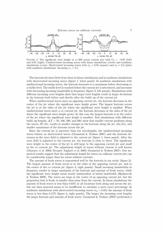
Extreme waves on collinear currents 7

Figure 2. The significant wave height at x=300 across current jets with U0 = −0.05 (left)and 0.05 (right). Unidirectional incoming waves with linear simulations (circle) and nonlinearsimulations (cross). Shortcrested incoming waves with σy = 0.05 (square) and σy = 0.2 (plus)with nonlinear simulations. Incoming σω = 0.1.

The kurtosis deviates little from three in linear simulations and in nonlinear simulationswith shortcrested incoming waves (figure 1, lower panel). In nonlinear simulations withunidirectional incoming waves, the kurtosis increases to a maximum before decreasing toa stable level. The stable level is reached before the current jet is introduced, and increaseswith decreasing incoming bandwidth in frequency (figure 3, left panels). Simulations withdifferent incoming crest lengths show that larger crest lengths result in larger deviationsin the kurtosis both before and shortly after the build–up of the current jet.

When unidirectional waves meet an opposing current jet, the kurtosis decreases in thecentre of the jet where the significant wave height grows. The largest kurtosis acrossthe jet is at the sides of the jet where the significant wave height is smallest. Whenunidirectional waves meet a co–current jet, the kurtosis decreases at the sides of the jetwhere the significant wave height grows. In this case the largest kurtosis is in the centreof the jet where the significant wave height is smallest. Test simulations with differentbuild–up lengths, ΔX = 50, 100, 200, and 300, show that smaller current gradients alongthe waves, ∂U/∂x, results in smaller changes in the kurtosis along the jet, |∂κ/∂x|, andsmaller maximums of the kurtosis across the jet.

Since the current jet is narrower than ten wavelengths, the unidirectional incomingwaves behave as shortcrested waves (Gramstad & Trulsen 2007) and the kurtosis de-creases as the wave field is adjusted to the current jet (figure 1, lower panel). After thewave field is adjusted to the current jet, the kurtosis is close to three. The significantwave height in the centre of the jet is still large in the opposing current jet and smallin the co–current jet. The adjustment length of waves without current is well known(Onorato et al. 2002; Socquet–Juglard et al. 2005; Gramstad & Trulsen 2007). Our nu-merical results suggest that the adjustment length for waves on collinear current jets canbe considerably longer than for waves without currents.

The amount of freak waves is represented well by the kurtosis in our study (figure 3).The largest amount of freak waves is at the sides of the opposing current jet, and inthe centre of the co–current jet (figure 3, right panels). Small incoming bandwidths infrequency results in larger maximum of the kurtosis and amount of freak waves, whilethe significant wave height seems nearly independent of initial bandwidth (Hjelmervik& Trulsen 2009). The waves are large in the centre of an opposing current jet, but theproportion that is freak, is smaller than away from the current. In linear simulations theamount of freak waves is less than 0.04% at all locations both along and across the jet,but our data material seems to be insufficient to calculate a more exact percentage. Innonlinear simulations with shortcrested incoming waves (σy = 0.05) the amount of freakwaves is less than 0.15% (figure 4, right panels). The longer the incoming crest lengthsthe larger kurtosis and amount of freak waves. Gramstad & Trulsen (2007) performed a

8 K. B. Hjelmervik and K. Trulsen

Figure 3. The kurtosis (left) and amount of local freak waves (right) for unidirectional incom-ing waves at x=300 across current jets with U0 = −0.05 (upper) and 0.05 (lower). Incomingσω = 0.05 (circle), 0.1 (cross) and 0.2 (square). Nonlinear simulations.

Figure 4. The kurtosis (left) and amount of local freak waves (right) for incoming shortcrestedwaves (σy = 0.05) at x=300 across current jets with U0 = −0.05 (upper) and 0.05 (lower).Incoming σω = 0.05 (circle), 0.1 (cross) and 0.2 (square). Nonlinear simulations.

large number of simulations with a modified nonlinear Schrodinger equation in order toreveal how the occurrence of freak waves on deep water depends on crest lengths. Theyfound a clear difference between shortcrested and longcrested waves, distinguished by alimiting crest length of approximately ten wavelengths (σy ≈ 0.1). Our results indicatethat a similar qualitative difference exists when a current jet is introduced. The longerthe crest lengths, the stronger the variations in significant wave height, kurtosis andamount of freak waves across the jet.

4.2. Space or time averaged significant wave heightOur definition of freak waves by (4.3) requires knowledge of the significant wave heightHs. Since the waves propagate in an inhomogeneous medium, there are at least three

Extreme waves on collinear currents 9

Figure 5. The amount of freak waves at x=300 for unidirectional incoming waves acrosscurrent jets with U0 = −0.05 (left) and 0.05 (right). Incoming σω = 0.1. Nonlinear simulations.

Figure 6. The amount of freak waves for unidirectional incoming waves with no current (——), and in the centre of current jets with U0 = −0.05 (——) and 0.05 (- - -). Incoming σω = 0.1.Nonlinear simulations.

different strategies for determining Hs. The strategy which we recommend and haveadopted here, is to determine Hs at fixed locations of constant current, i.e. a local sig-nificant wave height. This method corresponds to classical field measurements taken atfixed locations. A second strategy would be to determine a global significant wave heightby spatial averaging over the inhomogeneous medium. This method likely correspondsto analysis based on satellite imaging of the ocean surface. A third strategy would be todefine an undisturbed significant wave height for a wave field unaffected by the inhomo-geneities. This method corresponds to the work done by e.g. Lavrenov (1998).

Lavrenov (1998) considered the propagation of swell from the southern latitudes intothe opposing Agulhas current. He found that the mean wave height is larger in the centreof the jet than at the jet sides. Our simulations show that this applies for both linearand nonlinear simulations, and both unidirectional and shortcrested incoming waves. Hesuggested that the amount of freak waves is large in the centre of the jet since the meanwave height is large there.

Figures 5 and 6 show that the amount of “freak” waves strongly depends on thestrategy used to define them. The kurtosis is a good indicator for freak waves only ifthe local significant wave height is used to define them. Then the freak wave amount islarge at locations with a large amount of unexpectedly high waves compared to what isexpected at the same locations, and when the waves are adjusted to the current jet, thefreak wave amount is small. If the undisturbed significant wave height is used to definethe freak waves, the local significant wave height is a good indicator for the freak waveamount. Then the freak wave amount is large at locations with large waves compared towave heights elsewhere, and when the waves are adjusted to the current jet, the freakwave amount is still large. We believe it is preferrable to reserve the term “freak” wavesonly to those waves that are surprising even after knowledge of inhomogeneities are taken

10 K. B. Hjelmervik and K. Trulsen

Figure 7. The significant wave height (upper) and kurtosis (lower) for unidirectional and short-crested (σy = 0.05) incoming waves with no current (— —), and on transversally uniformcurrents with U0 = −0.05 (——) and 0.05 (- - -). Incoming σω = 0.1. Nonlinear simulations.

Figure 8. The amount of freak waves for unidirectional incoming waves with no current (— —),and on transversally uniform currents with U0 = −0.05 (——) and 0.05 (- - -). Incomingσω = 0.1. Nonlinear simulations.

into account. To ensure that a freak wave belongs to the upper tail of the probabilitydistribution, we thus recommend the local significant wave height for application to thecriterion (4.3).

4.3. Transversally uniform current

Suppose that the waves meet a transversally uniform current given by (3.5).The significant wave height (figure 7, upper panel) increases when the waves meet

an increasing opposing current and decreases when the waves meet an increasing co–current. Since the current does not cause any energy transfer transversally, the changes

Extreme waves on collinear currents 11

are smaller than when the waves meet a current jet (figure 1, upper panel). The significantwave height is near constant after the build–up of the current.

The kurtosis (figure 7, lower panel) for longcrested waves increases slightly when thesignificant wave height increases, and decreases slightly when the significant wave heightdecreases. This effect can hardly be seen for short crested waves. After the current build–up the unidirectional incoming waves are still unidirectional and the kurtosis stays at thesame level. This is in contradiction to the case where unidirectional incoming waves meeta current jet (figure 1, lower panel). Then the kurtosis decreases with increasing signif-icant wave height, increases with decreasing significant wave height, and decreases afterthe build–up. The kurtosis for unidirectional incoming waves with no current (figures 1and 7, lower panels) stays at a high level, indicating that the cubic nonlinear Schrodingerequation produces larger kurtosis than the modified Schrodinger equation by Trulsen &Dysthe (1996) derived to next order (see Gramstad & Trulsen 2007, figure 2).

On a transversally uniform current the amount of freak waves (figure 8) is well indicatedby the kurtosis also when the undisturbed significant wave height is used to calculatethe amount of freak waves. If the undisturbed significant wave height is used, there areslightly more freak waves in an opposing current and less in a co–current, than if thelocal significant wave height is used. Since the current does not introduce transversalenergy transfer, the freak wave amounts are smaller than if the waves meet a current jet(figure 5).

5. ConclusionWe have derived a nonlinear Schrodinger equation suitable for spatial wave propagation

on inhomogeneous currents. We have used this equation for Monte–Carlo simulations toinvestigate wave statistics on inhomogeneous currents, in particular on narrow currentjets. Several surprising features of nonlinear wave evolution on nonuniform current wererevealed. Wave statistics has been derived based on the envelope to the first order, whichwas used to estimate the wave height correct to second order.

The evolution and statistics of both short– and longcrested waves on transversallyuniform currents is found to be qualitatively different from waves on current jets.

Considering waves that approach an opposing current jet, we find that the amount offreak waves is minimum in the centre of the jet where the wave heights are largest, whilethe amount of freak waves is maximum at the sides of the jet where the wave heights aresmallest.

The definition of both significant wave height and of freak waves can be ambiguous ininhomogeneous media. We recommend that local definitions are used to ensure that freakwaves remain surprising even after classical knowledge of the inhomogeneous medium hasbeen taken into account.

We see evidence that the distances over which a wave field has to propagate in orderto be adjusted to the medium can become much longer in the presence of inhomogeneouscurrents than in the absence of currents. This may be an important consideration for theappropriate choice of wave models in coastal waters.

We thank professors Kristian B. Dysthe and Bjørn Gjevik for fruitful discussions.Several referees provided useful comments on preliminary versions of the manuscript.

K.T. is grateful for the hospitality of the Department of Signal Theory and Commu-nications at the Polytechnic School at the University of Alcala, Spain, for hosting himduring a sabbatical year during the development of this paper.

12 K. B. Hjelmervik and K. Trulsen

Appendix. Derivation of the NLSC equationTaylor expansions around z = 0 gives the surface boundary equations, (2.2a–b), on

the form:

∂η

∂t+ vtot · ∇(η + ζ) + (η + ζ)

∂vtot

∂z· ∇(η + ζ) +

12(η + ζ)2

∂2vtot

∂z2· ∇(η + ζ)

= w + W + (η + ζ)∂

∂z(w + W ) +

12(η + ζ)

∂2

∂z2(w + W ) + · · · (A 1a)

ptot + (η + ζ)∂ptot

∂z+

12(η + ζ)2

∂2ptot

∂z2+ · · · = pa (A 1b)

The waves are assumed on deep water, that is v, p → 0 as z → −∞.In accordance with the scaling assumptions from section 2, all equations, variables and

sizes in the following are made dimensionless using the characteristic length and timescales of the wave field, so that kcx → x, εkcx → x, ωct → t, kcη → εη, kcζ → ε2ζ,kc

ωcu → εu, kc

ωc(U, V ) → ε(U, V ), kc

ωcW → ε2W , kc

ρg p → εp, and kc

ρg P → ε2P .The scaled Euler equation for the waves (2.1) to the third order of ε is:

∂u

∂t+ ε

(U

∂u

∂x+ V

∂u

∂y+ v · ∇u

)+ ε2

(u

∂U

∂x+ v

∂U

∂y+ W

∂u

∂z

)= − ∂p

∂x(A 2a)

∂v

∂t+ ε

(U

∂v

∂x+ V

∂v

∂y+ v · ∇v

)+ ε2

(u

∂V

∂x+ v

∂V

∂y+ W

∂v

∂z

)= −∂p

∂y(A 2b)

∂w

∂t+ ε

(U

∂w

∂x+ V

∂w

∂y+ v · ∇w

)+ ε2W

∂w

∂z= −∂p

∂z(A 2c)

The scaled equation for the divergence of the Euler equation for the waves (2.1) to thethird order of ε is:

ε

((∂u

∂x

)2

+(

∂v

∂u

)2

+(

∂w

∂z

)2

+ 2∂u

∂y

∂v

∂x+ 2

∂u

∂z

∂w

∂x+ 2

∂v

∂z

∂w

∂y

)

+2ε2(

∂u

∂x

∂U

∂x+

∂u

∂y

∂V

∂x+

∂v

∂x

∂U

∂y+

∂v

∂y

∂V

∂y

)= − ∂2p

∂x2− ∂2p

∂y2− ∂2p

∂z2(A 3)

The scaled surface equations for the waves (A 1a–b) to the third order of ε are:

∂η

∂t+ ε(v + V ) · ∇η + ε2η

∂v

∂z· ∇η = w + εη

∂w

∂z+ ε2

(ζ∂w

∂z+

12η2 ∂2w

∂z2

)(A 4a)

p− η + εη∂p

∂z+ ε2

(ζ∂p

∂z+

12η2 ∂2p

∂z2

)= 0 (A4b)

The wave field is represented by perturbation series for the surface displacement, η,the velocity, v, and the dynamic pressure, p:

η = ε2η + 12

(B1ei(x−t) + εB2e2i(x−t) + · · ·+ c.c.

)v = ε2v + 1

2

(v1 ei(x−t) + εv2 e2i(x−t) + · · ·+ c.c.

)p = εp + 1

2

(p1 ei(x−t) + εp2 e2i(x−t) + · · ·+ c.c.

) (A 5)

We shall assume that the waves are modulated on the slow spatial scales x and y anda correspondingly slow time scale εt = t. Thus η = η(x, y, t), v = v(x, y, z, t), andp = p(x, y, z, t) are the mean surface displacement, mean induced velocity, and meandynamic pressure respectively, while Bn = Bn(x, y, t), vn = vn(x, y, z, t), and pn =

Extreme waves on collinear currents 13

pn(x, y, z, t) are the n’th harmonics of the surface displacement, induced current, anddynamic pressure respectively. The characteristic wavenumber is fixed appropriate forwaves undisturbed by current, therefore the entire effect of refraction is represented bythe modulation of B1.

The horizontal vorticities and the vertical vorticity are all one order higher than thevorticities used by Mei (1989), that is (Γx, Γy) = O(ε3) and Γz = O(ε2). Since thevorticity is assumed to be small, the chosen order of the mean functions are supportedby Dysthe (1979). Both the mean functions and the harmonics, are perturbed:

η = η2 + · · · , Bn = Bn0 + εBn1 + ε2Bn2 + · · ·v = v2 + · · · , vn = vn0 + εvn1 + ε2vn2 + · · ·p = p1 + εp2 + · · · , pn = pn0 + εpn1 + ε2 pn2 + · · ·

(A 6)

A.1. First order termsThe first harmonic terms of first order of ε for the divergence of the Euler equation (A 3)are:

p10 − ∂2p10

∂z2= 0 (A 7)

which has the general solution:

p10 = A10(x, y, t)ez (A 8)

The first harmonic terms of first order of ε in the surface equations (A 4a–b) give:

A10 = B10 (A 9)

The first harmonic terms of first order of ε in the Euler equation (A 2a–c) then giverespectively:

u10 = B10ez (A 10a)v10 = 0 (A 10b)w10 = −iB10ez (A 10c)

A.2. Second order termsA.2.1. Zeroth harmonic

The zeroth harmonic terms of second order of ε for the z–component of the Eulerequation (A 2c) are:

i4u10w

∗10 +

i4u∗10w10 +

14w10

∂w∗10∂z

+14w∗10

∂w10

∂z= −∂p1

∂z(A 11)

Using the results (A 10) from first order, gives:

|B10|2e2z = −∂p1

∂z(A 12)

which has the solution:

p1 = A1(x, y, t)− 12|B10|2e2z (A 13)

The zeroth harmonic terms of second order of ε in the dynamic surface equation (A 4b)are:

p1 +14B10

∂p∗10∂z

+14B∗10

∂p10

∂z= 0 at z = 0 (A14)

Using the results (A 8–A9) from first order and the solution for p1 (A 13), gives A1 = 0.

14 K. B. Hjelmervik and K. Trulsen

A.2.2. First harmonic

The first harmonic terms of second order of ε for the divergence of the Euler equation(A 3) are:

2i∂p10

∂x= p11 − ∂2p11

∂z2(A 15)

Using the results (A 8–A9) from leading order, gives:

2i∂B10

∂xez = p11 − ∂2p11

∂z2(A 16)

which has the solution:

p11 = A11(x, y, t)ez − i∂B10

∂xzez (A 17)

The first harmonic terms of second order of ε in the dynamic surface equation (A 4b)give:

A11 = B11 (A 18)

The first harmonic terms of second order of ε in the Euler equation and the kinematicsurface equation (A 2a–c, A 4a) are respectively:

∂u10

∂t− iu11 + iu10U = −∂p10

∂x− ip11 (A 19a)

∂v10

∂t− iv11 + iv10U = −∂p10

∂y(A 19b)

∂w10

∂t− iw11 + iw10U = −∂p11

∂z(A 19c)

∂B10

∂t− iB11 + iUB10 = w11 at z = 0 (A 19d)

Using the results (A 8–A10) from first order and the solution for p11 (A 17–A18), leadsto the current modified Schrodinger equation to second order:

∂B10

∂x+ 2

∂B1,0

∂t+ 2iUB10 = 0 (A20)

and the reconstruction formulas:

u11 = B11ez + i(

∂B10

∂t+ iUB10

)(1 + 2z)ez (A 21a)

v11 = −i∂B10

∂yez (A 21b)

w11 = −iB11ez +(

∂B10

∂t+ iUB10

)(1 + 2z)ez (A 21c)

A.2.3. Second harmonic

The second harmonic terms of second order of ε for the divergence of the Euler equation(A 3) are:

−12u2

10 +12

(∂w10

∂z

)2

+ i∂u10

∂zw10 = 4p20 − ∂2p20

∂z2(A 22)

Extreme waves on collinear currents 15

Using the results (A 10) from leading order, gives:

0 = 4p20 − ∂2p20

∂z2(A 23)

which has the solution:

p20 = A20e2z (A 24)

The second harmonic terms of second order of ε in the dynamic surface equation (A 4b)are:

p20 −B20 +12B10

∂p10

∂z= 0 at z = 0 (A25)

Using the results (A 8–A9) from leading order and the solution for p20 (A 24), gives:

A20 = B20 − 12B2

10 (A 26)

The second harmonic terms of second order of ε in the Euler equation and the kinematicsurface equation (A 2a–c, A 4) are respectively:

−iu20 +i4u2

10 +14w10

∂u10

∂z= −ip20 (A 27a)

−iv20 +i4u10v10 +

14w10

∂v10

∂z= 0 (A 27b)

−iw20 +i4u10w10 +

14w10

∂w10

∂z= −1

2∂p20

∂z(A 27c)

−iB20 +i4u10 =

12w20 +

14B10

∂w10

∂zat z = 0 (A 27d)

Using the results (A 10) from first order and the solution for p20 (A 24, A 26), gives:

u20 = v20 = w20 = p20 = 0 (A 28a)

B20 =12B2

10 (A 28b)

Note that the second order contributions is not explicit functions of the current field.

A.3. Third order termsThe first harmonic terms of third order of ε for the divergence of the Euler equation (A 3)are:

u20u∗10 +

12

∂w20

∂z

∂w∗10∂z

− i2

∂u20

∂zw∗10 + i

∂u∗10∂z

w20 + iu10∂U

∂x+ iv10

∂U

∂y

= −12

∂2p10

∂x2− i

∂p11

∂x+

12p12 − 1

2∂2p10

∂y2− 1

2∂2p12

∂z2(A 29)

Using the results (A 8–A10, A 17–A18, A 28) from first and second order, gives:

∂2p12

∂z2− p12 = −2i

∂B11

∂xez − ∂2B10

∂x2ez − ∂2B10

∂y2ez − 2

∂2B10

∂x2zez − 2iB10

∂U

∂xez

(A 30)

which has the solution:

p1,2 = A12(x, y, z, t)ez + α(x, y, z, t)zez + β(x, y, t)z2ez (A 31)

16 K. B. Hjelmervik and K. Trulsen

where

α = −i∂B11

∂x− 1

2∂2B10

∂y2− iB10

∂U

∂x

β = −12

∂2B10

∂x2

The first harmonic terms of third order of ε in the dynamic surface equation (A 4b)are:

12p12 − 1

2B12 +

14B20

∂p∗10∂z

+14B∗10

∂p20

∂z+

12B10

∂p1

∂z

+12ζ∂p10

∂z+

116

B210

∂2p∗10∂z2

+18|B10|2 ∂2p10

∂z2= 0 at z = 0 (A32)

Using the results (A 8–A9, A 13, A 28–A28) from first and second order, and the solutionfor p12 (A 31), gives:

A12 = B12 +38B2

10B∗10 −B10ζ at z = 0 (A33)

The first harmonic terms of third order of ε in the Euler equation and the kinematicsurface equation (A 2a–c, A 4a) are respectively:

12

∂u11

∂t− i

2u12 +

12

∂u10

∂xU +

i2u11U +

12

∂u10

∂yV +

12u10W +

12u10

∂U

∂x+

12v10

∂U

∂y

− i4u20u

∗1,0 +

i2u∗10u20 +

14w20

∂u∗10∂z

+14w∗10

∂u20

∂z= −1

2∂p11

∂x− i

2p12 (A 34a)

12

∂v11

∂t− i

2v12 +

12

∂v10

∂xU +

i2v11U +

12

∂v10

∂yV +

12v10W +

12u10

∂V

∂x+

12v10

∂V

∂y

− i4u20v

∗10 +

i2u∗10v20 +

14w20

∂v∗10∂z

+14w∗10

∂v20

∂z= −1

2∂p11

∂y(A 34b)

12

∂w11

∂t− i

2w12 +

12

∂w10

∂xU +

i2w11U +

12

∂w10

∂yV +

12w10W

− i4u20w

∗10 +

i2u∗10w20 +

14w20

∂w∗10∂z

+14w∗10

∂w20

∂z= −1

2∂p12

∂z(A 34c)

12

∂B11

∂t− i

2B12 − i

4u20B

∗10 +

i2u∗10B20 +

i2B11U

+12

∂B10

∂xU +

12

∂B10

∂yV +

i8B2

10

∂u∗10∂z

=12w12 +

14B20

∂w∗10∂z

+12B∗10

∂w20

∂z+

12ζ∂w10

∂z

+116

B210

∂w∗10∂z

+18|B10|2 ∂2w10

∂z2at z = 0 (A 34d)

Combining these equations with the results (A 10, A 17–A18, A 21, A 28) from first andsecond order, and the solution for p12 (A 31, A 33), gives:

0 =∂B11

∂x+ 2

∂B11

∂t+ i

∂2B10

∂t2− i

2∂2B10

∂y2+ iB2

10B∗10

+2iB11U − 6∂B10

∂tU − 5iB10U

2 + 2∂B10

∂yV + B10

∂U

∂x(A 35)

which combined with (A 20) leads to the space evolution of the current modified cubic

Extreme waves on collinear currents 17

nonlinear Schrodinger equation, NLSC, (2.5) where B = B1 and the bars are dropped tosimplify the notation.

More on the derivation of the NLSC equation can be found in Hjelmervik & Trulsen(2009).

REFERENCES

Bottin, R. R. Jr. & Thompson, E. F. 2002 Comparisons of physical and numerical modelwave predictions with prototype data at Morro Bay harbor entrance, California. U. S. ArmyEngineer.

Dysthe, K. B. 1979 Note on the modification to the nonlinear Schrodinger equation for appli-cation to deep water waves. Proc. R. Soc. Lond. A 369, 105–114.

Dysthe, K. B., Krogstad, H. E. & Muller, P. 2008 Oceanic Rogue Waves. Annu. Rev.Fluid Mech. 40, 287–310.

Gerber, M. 1987 The Benjamin–Feir instability of a deep water Stokes wavepacket in thepresence of a non–uniform medium. J. Fluid Mech. 176, 311–332.

Gonzalez, F. I. 1984 A case study of wave–current–bathymetry interactions at the Columbiariver entrance. J. Phys. Oceanogr. 14, 1065–1078.

Gramstad, O. & Trulsen, K. 2007 Influence of crest and group length on the occurrence offreak waves. J. Fluid Mech. 582, 463–472.

Hjelmervik, K., Ommundsen, A. & Gjevik, B. 2005 Implementation of non–linear advectionterms in a high resolution tidal model. University of Oslo, preprint.

Hjelmervik, K., Lynge, B. K., Ommundsen, A. & Gjevik, B. 2008 Interaction of tides andstorm surges in the Tjeldsunet channel in northern Norway. Ocean Dynamics (submitted).

Hjelmervik, K. & Trulsen, K. 2009 The current modified nonlinear Schrodinger equationwhich allows vorticity. University of Oslo, preprint, (to be submitted).

Jonsson, I. G. 1990 Wave–current interactions. In The Sea, Ocean Eng. Sci. (ed. by B. LeMhaut & D. M. Hanes), pp. 65–120, Wiley-Interscience, Hoboken, N. J.

Kharif, C. & Pelinovsky, E. 2003 Physical mechanisms of the rogue wave phenomenon. Eur.J. Mech. B/Fluids 22, 603–634.

Lavrenov, I. V. 1998 The wave energy concentration at the Agulhas current off South Africa.Natural Hazards 17, 117–127.

Lavrenov, I. V. & Porubov, A. V. 2006 Three reasons for freak wave generation in thenon–uniform current. Eur. J. Mech. B/Fluids 25, 574–585.

Lo, E. Y. & Mei, C. C. 1985 A numerical study of water–wave modulation based on a higher–order nonlinear Schrodinger equation. J. Fluid Mech. 150, 395–416.

Longuet–Higgins, M. S. & Stewart, R. W. 1961 The changes in amplitude of short gravitywaves on steady non–uniform currents. J. Fluid Mech. 10, 529–549.

MacIver, R. D., Simons, R. R. & Thomas, G. P. 2006 Gravity waves interacting with narrowjet–like current. J. Geophys. Res. 111, C03009.

MacMahan, J. H., Thornton, E. B. & Reniers, A. J. H. M. 2006 Rip current review.Coastal Engineering 53, 191–208.

Mei, C. C. 1989 The applied dynamics of ocean surface waves. World Scientific Publishing Co.,Singapore., ISBN 9971–50–789–7

Mori, N., Liu, P. C. & Yasuda, T. 2002 Analysis of freak wave measurements in the sea ofJapan. Ocean Engineering 29, 1399–1414.

Muslu, G. M. & Erbay, H. A. 2004 Higher–order split–step Fourier schemes for the generalizednonlinear Schrodinger equation. Mathematics and Computers in Simulation 67, 581–595.

Onorato, M., Osborne, A. R., Serio, M., Resio, D., Pushkarev, A., Zakharov, V. E.

& Brandini, C. Freely decaying weak turbulence for sea surface gravity waves. Phys. Rev.Lett. 89, 144501.

Peregrine, D. H. 1976 Interaction of water waves and currents. Adv. Appl. Mech. 16, 9–117.

Peregrine, D. H. & Smith, R. 1979 Nonlinear effects upon waves near caustics. Phil. Trans.R. Soc. Land. A 292, 341–370.

Socquet–Juglard, H., Dysthe, K. B., Trulsen, K., Krogstad, H. E. & Liu, J. 2005

18 K. B. Hjelmervik and K. Trulsen

Probability distributions of surface gravity waves during spectral changes. J. Fluid. Mech.542 195–216.

Stewartson, K. 1977 On the resonant interaction between a surface wave and a weak surfacecurrent. Mathematika 24, 37–49.

Stocker, J. D. & Peregrine, D. H. 1999 The current–modified nonlinear Schrodinger equa-tion. J. Fluid Mech. 399, 335–353.

Tayfun, M. A. 1980 Narrow-band nonlinear sea waves. J. Geophys. Res. 85, 1548–1552.Trulsen, K. & Dysthe, K. B. 1996 A modified nonlinear Schrodinger equation for broader

bandwidth gravity waves on deep water. Wave Motion 24, 281–289.Turpin, F–M., Benmoussa, C. & Mei, C. C. 1983 Efects of slowly varying depth and current

on the evolution of a Stokes wavepacket. J. Fluid Mech. 132, 1–23.White, B. S. & Fornberg, B. 1998 On the chance of freak waves at sea. J. Fluid Mech. 335,

113–138.White, B. S. 1999 Wave action on currents with vorticity. J. Fluid Mech. 386, 329–344.Wu, C. H. & Yao A. 2004 Laboratory measurements of limiting freak waves on currents.

J. Geophys. Res. 109, C12002.Zakharov, V. E. 1968 Stability of periodic waves of finite amplitude on the surface of a deep

fluid. J. Appl. Mech. Tech. Phys. 9, 86–94.