waveeld extrapolation in phase-ray coordinatessep · waveeld extrapolation in phase-ray coordinates...

Stanford Exploration Project, Report 114, October 14, 2003, pages 31–44

Wavefield extrapolation in phase-ray coordinates

Jeff Shragge and Biondo Biondi1

ABSTRACT

A ray theoretic formulation is developed that allows rays to be traced directly from exist-ing solutions to the Helmholtz equation. These rays, termed phase-rays, are defined bythe direction normal to surfaces of constant wavefield phase. Phase-rays exhibit a num-ber of attractive characteristics, including triplication-free ray-fields, an ability to shootrays forward or backward, and an ability to shoot infill rays for ensuring adequate raydensity. Because of these traits, we use phase-rays as a coordinate basis on which toextrapolate wavefields using the generalized coordinate system approach. Examples ofwavefields successfully extrapolated in phase-ray coordinates are presented, and the mer-its and drawbacks of this approach, relative to conventionally traced ray coordinates, arediscussed.

INTRODUCTION

Ray theory is routinely applied to generate characteristics to solutions of the Helmholtz equa-tion. The usual ray theoretic approach introduces an ansatz representation of the wavefield so-lution into the Helmholtz equation to yield coupled eikonal and transport equations. Computa-tion of eikonal equation solutions is usually facilitated by the introduction of a high-frequencyapproximation that removes the amplitude dependence from the full eikonal equation. Conse-quently, conventionally computed rays are independent of frequency and often triplicate dueto their broad-band nature.

In contrast, whenever independent solutions to the Helmholtz equation exist, full ray the-oretic formulae may be used to trace rays (Foreman, 1989). These rays are termed phase-raysherein owing to a ray direction that is always orthogonal to surfaces of constant phase. Oneof their beneficial traits is that, unlike conventionally traced rays, computed ray-fields arecaustic-free. A second advantage is that ray position is the only required initial condition forray-tracing. However, one obstacle seems to restrict the use of the phase-ray formulation inseismic imaging problems: wavefield solutions to the Helmholtz equation must be known inadvance of ray-field computation.

One situation where phase-rays (and conventional rays) are of use is in wavefield extrap-olation in generalized (i.e. non-Cartesian) coordinates (Sava and Fomel, 2003). A naturalset of coordinates for wavefield extrapolation is the general ray family represented by a ray

1email: [email protected], [email protected]

31

32 Shragge and Biondi SEP–114

direction and shooting angle(s). Wavefield extrapolation in ray coordinates thus uses a ray-field as the coordinate system on which to extrapolate wavefields. This approach transformsthe physics of one-way wave propagation from the usual Cartesian grid so that it is valid ina ray coordinate system. Wavefield extrapolation operators are then applied more accuratelybecause extrapolation can occur at lower angles to the ray direction than usually occurs withCartesian coordinates. The result is then mapped from ray coordinates to Cartesian. Althoughray domain extrapolated wavefields are generally more accurate, issues still remain when us-ing conventionally-traced rays; in particular, how to robustly deal with infinite amplitudes atlocations of coordinate system triplication.

Motivated by this issue, this paper examines the use of phase-rays as a coordinate systemfor wavefield extrapolation. The main advantage of phase-ray coordinates is that they arecaustic-free, and thereby avoid complications arising from triplicating coordinates. The paperbegins with a general discussion of ray theory and an approach for calculating phase-raysfrom solutions to the Helmholtz equation. Phase-ray examples from a salt body model arethen presented, and are followed by results illustrating wavefield extrapolation in phase-raycoordinates for a Gaussian velocity perturbation model. Finally, a method is proposed forpropagating broadband wavefields using frequency-dependent phase-ray coordinates.

THEORY

The theory outlined in this section closely follows that of Foreman’s exact ray theory (Fore-man, 1989), but is summarized here for completeness. Ray theory may be used to computethe characteristics to the time-independent, homogeneous Helmholtz equation,

∇29 + k29 = 0, (1)

where 9 is the desired wavefield solution, and k is the wavenumber. In most ray theoreticdevelopments, the wavefield is represented by an ansatz solution, 9 = Aeiφ , where A(r) andφ(r) are the amplitude and phase functions, respectively. Substituting this representation intothe Helmholtz equation yields the usual eikonal and transport equations,

K 2 = K ·K = ∇φ ·∇φ = k2 +∇2 A

A, (2)

2∇ A ·∇φ + A∇2φ = 0,

where K is the phase gradient vector (see figure 1). Solutions to equations (2) are the raypaths and the amplitudes along these ray paths, respectively. In isotropic media the gradientof the phase function, K = ∇φ, is orthogonal to surfaces of constant phase and represents theinstantaneous direction of propagation. Explicitly, this may be written,

K = ∇φ = |K |dds

r, (3)

where ds is an element of length, and dr is a vector element of the ray-path. A ray-pathequation is developed by taking the gradient of the phase gradient magnitude (i.e. ∇K ),

K 2 = K ·K,

SEP–114 Phase-rays 33

Figure 1: Schematic of phase-frontgradient quantities. K is the phasegradient vector, |K |ds is the gra-dient magnitude along step ds, and|K |dx and |K |dz are the projectionsof |K |ds along the x and z coordi-nates, respectively. jeff1-Rays [NR]

X

Z

Phase Front

|K|ds |K|dz

|K|dxK=|K|r

2K∇K = 2(K ·∇)K+2K× (∇ ×K) ,∇K =

[

(K/K ·∇]

K, (4)

=

(

dds

r ·∇

)

K =dds

K,

where ∇ × K = ∇ × ∇φ = 0 has been employed. Using equation (3) this may be writtenexplicitly,

∇K =dds

(

Kdds

r)

(5)

Coupling between the eikonal and transport equations is evident through the dependence ofthe eikonal equation on amplitude function, A. In many cases a high-frequency approximation(i.e. ∇2 A

A ≈ 0) is used to decouple these equations. Use of this approximation yields the usualform of the ray path equation,

dds

(

1c

dds

r)

= ∇

(

1c

)

, (6)

where c is the velocity. Use of this approximation also eliminates the frequency dependenceof ray trajectories (see Appendix A). One manner of reintroducing frequency-dependent raytrajectories is discussed in a latter section.

Phase-ray formulation

When a solution, 9, to the Helmholtz equation is known, obtaining a ray trajectory usingequation (5) is relatively trivial. The expression for the wavefield gradient, ∇9 = ∇(Aeiφ),divided by the wavefield, 9, is,

∇9

9=

∇ AA

+ iK. (7)

An expression for the wavefield gradient vector, K, is obtained by retaining the imaginarycomponent of equation (7) and using the expression for K in equation (3),

Kdds

r = Im(

∇9

9

)

(8)


Equation (8) may be rewritten explicitly as a system of two decoupled ordinary differentialequations,

dds

[

xz

]

=1

√

( ∂9∂x )2 + ( ∂9

∂z )2Im

(

19

[

∂∂x∂∂z

]

9

)

. (9)

The solution for ray-path, r, is computed through an initial evaluation of the right hand side ofequations (9), and an iterative forward step by a constant interval using the precomputed quan-tity to determine the proper apportioning of the step along each coordinate. Note that becausethese differential equations are first-order, only one initial condition (position) is required forray computation, and rays may be started from any location in the wavefield solution. Finally,although the two-dimensional formulation is presented here, the extension to three dimensionsis trivial.

PHASE-RAY EXAMPLES

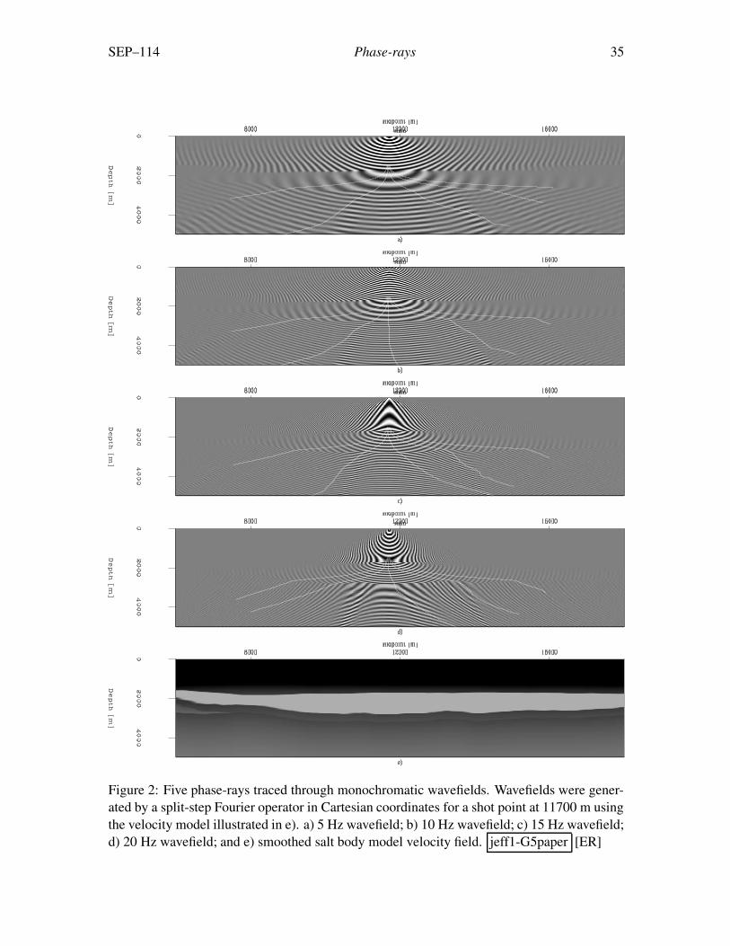
Examples of traced phase-rays are presented in this section using a salt body velocity field asa didactic model. The background velocity of the model, shown in figure 2e, is a typical Gulfof Mexico v(z) velocity gradient. The superposed salt body is characterized by higher wavespeeds (4700 m/s) and a fairly rugose bottom of salt interface.

Figure 2 presents five phase-rays computed from four different monochromatic wavefields.The wavefields were generated for a shot point located at 11700 m using a split-step Fourieroperator (Stoffa et al., 1990) in a Cartesian coordinate system. Each ray begins at the samepoint in all panels. The rays to the extreme left and right in each panel show little variabilityin their spatial location; however, the three remaining rays are attracted to regions of greaterwavefield amplitude and their spatial locations vary with a range up to 2000 m. Accordingly,because rays originate at the same spot, observed phase-ray movement is caused by changesin wavefield solution and indicates frequency-dependent behavior.

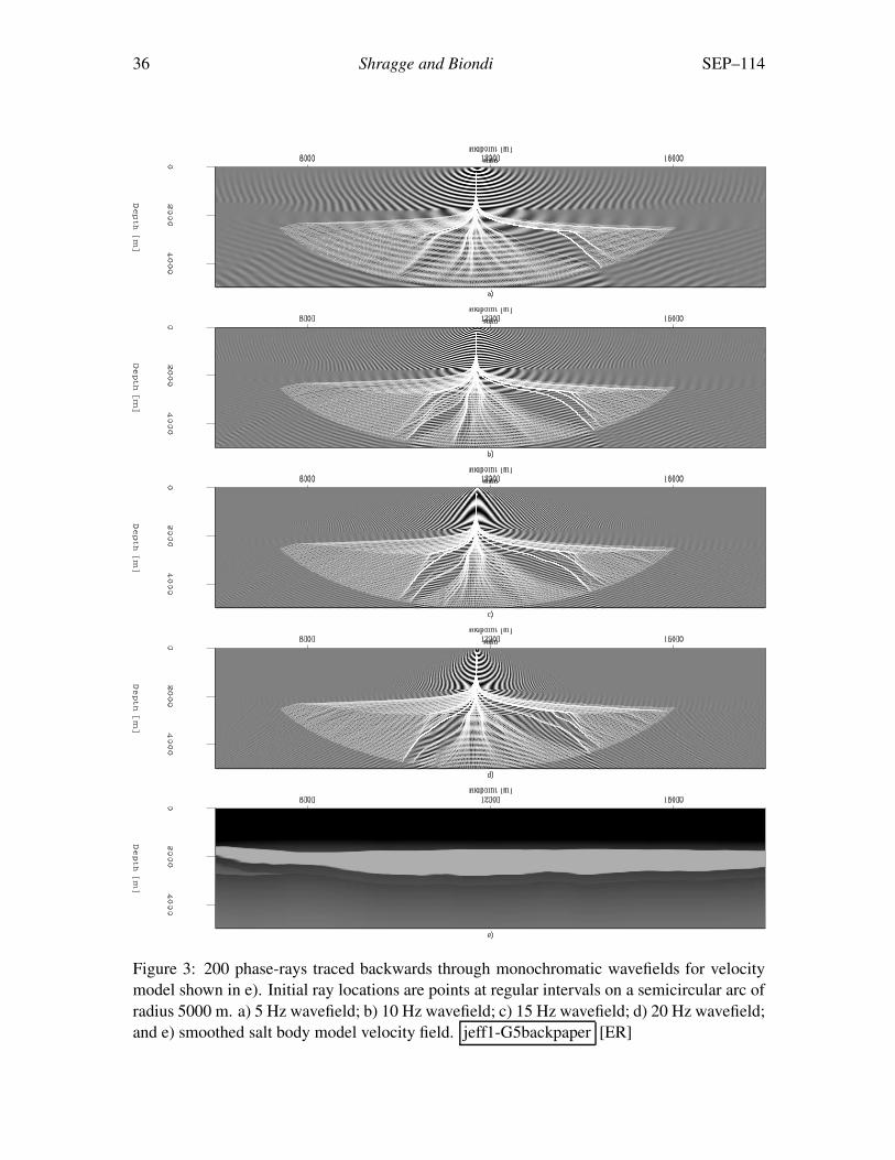
Phase-rays computed according to equations (9) may be traced in reverse, from observationto source point, by using a negative step interval. Figure 3 illustrates this situation with thesame model as in figure 2. Initial ray locations are points at regular intervals on a semicirculararc of radius 5000 m. Calculated phase-rays do not overlap and the ray-field is caustic-free.Phase-ray density, though, is frequency-dependent, with significant coverage gaps of variablesize appearing in all four panels. This suggests that an additional condition is required toensure that, when needed, ray density is more uniform. One solution is to shoot a new raybetween two successive rays wherever intra-ray distance exceeds some threshold value.

In summary, these results illustrate a number of advantageous characteristics of phase-rays: i) phase-ray ray-fields are triplication-free; ii) ray tracing from areas of low wavefieldamplitude (e.g. shadow zones) to the source point is possible; and iii) sufficient phase-raydensity may be ensured by an additional shooting of phase-rays wherever intra-ray spacing istoo large. These three traits provide the main impetus for using phase-ray coordinates as ageneralized coordinate system for wavefield extrapolation (Sava and Fomel, 2003).


Figure 2: Five phase-rays traced through monochromatic wavefields. Wavefields were gener-ated by a split-step Fourier operator in Cartesian coordinates for a shot point at 11700 m usingthe velocity model illustrated in e). a) 5 Hz wavefield; b) 10 Hz wavefield; c) 15 Hz wavefield;d) 20 Hz wavefield; and e) smoothed salt body model velocity field. jeff1-G5paper [ER]


Figure 3: 200 phase-rays traced backwards through monochromatic wavefields for velocitymodel shown in e). Initial ray locations are points at regular intervals on a semicircular arc ofradius 5000 m. a) 5 Hz wavefield; b) 10 Hz wavefield; c) 15 Hz wavefield; d) 20 Hz wavefield;and e) smoothed salt body model velocity field. jeff1-G5backpaper [ER]


WAVEFIELD EXTRAPOLATION IN PHASE-RAY COORDINATES

This section examines the use of phase-rays as a coordinate system for wavefield extrapolation.The velocity model examined here (shown in figure 4a) is characterized by a slow, Gaussian-shaped velocity anomaly (-600 m/s) in a medium of otherwise constant velocity (1200 m/s).This model was chosen to ensure that extrapolated wavefields triplicate, as illustrated by figure4b. This wavefield was generated for a shot point located at 8000 m using a split-step Fourieroperator in a Cartesian coordinate system. Figure 4c shows phase-rays traced through thewavefield of figure 4b. Phase-rays in the upper portions of the model have fairly smoothcoverage. In areas of wavefield triplication, though, significant coverage gaps are noticeable.

The phase-rays shown in figure 4c were subsequently used as a coordinate system for thegeneralized coordinate wavefield extrapolation approach (Sava and Fomel, 2003). Figure 5ashows the velocity model of figure 4a in phase-ray coordinates. Figure 5b presents the resultsof wavefield extrapolation in phase-ray coordinates using a split-step Fourier operator and thevelocity model shown in figure 5a. Figure 5c shows this result mapped to Cartesian coor-dinates. The wavefield presented in figure 5d was computed in Cartesian coordinates usinga split-step Fourier operator. In areas where wavefields are present in significant amplitude,the phase-ray and Cartesian results are similar. Areas of low wavefield amplitude beneaththe Gaussian velocity anomaly (e.g. [z,x]=[4200 m,6800 m]), though, are markedly different.This difference is related to the inability to map the results from ray coordinates to Cartesianin areas of minimal or non-existent ray coverage.

This experiment highlights a consequence of using phase-ray coordinates for wavefieldextrapolation. Monochromatic wavefield triplication is generally identified by interferencepatterns created by converging wavefield components. (See, for example, the checkerboardpattern beneath the Gaussian velocity anomaly.) Because phase-ray direction is dependenton the total wavefield gradient, it is similarly dependent on the gradients of each converg-ing wavefield component. The gradient vector, being unable to unwrap individual convergentphases, chooses a weighted average of individual gradients. Accordingly, phase-rays are usu-ally steered in the direction of the convergent component with the largest individual gradientmagnitude, but they will never triplicate since the weighted gradient is uniquely defined at eachwavefield point. This fact suggests that phase-ray coordinates represent a trade off betweenintroducing inaccuracy associated with triplicating coordinates and inaccuracy of wavefieldextrapolation at greater angles to the phase-ray direction.

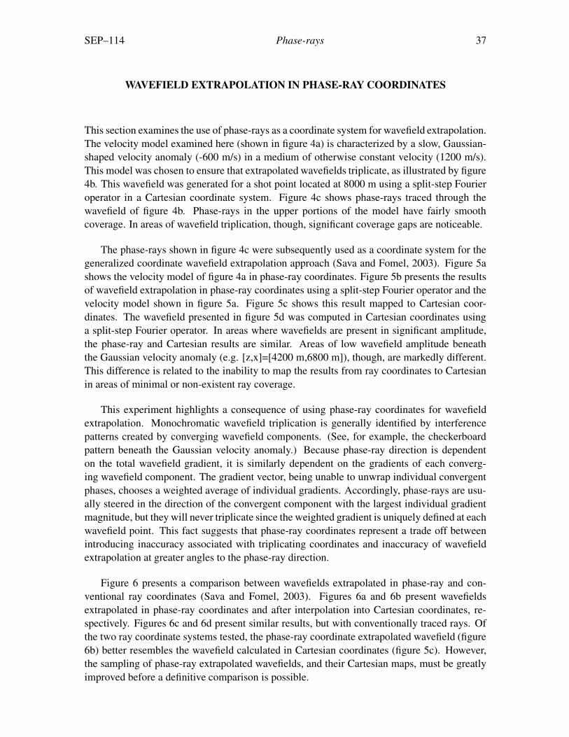
Figure 6 presents a comparison between wavefields extrapolated in phase-ray and con-ventional ray coordinates (Sava and Fomel, 2003). Figures 6a and 6b present wavefieldsextrapolated in phase-ray coordinates and after interpolation into Cartesian coordinates, re-spectively. Figures 6c and 6d present similar results, but with conventionally traced rays. Ofthe two ray coordinate systems tested, the phase-ray coordinate extrapolated wavefield (figure6b) better resembles the wavefield calculated in Cartesian coordinates (figure 5c). However,the sampling of phase-ray extrapolated wavefields, and their Cartesian maps, must be greatlyimproved before a definitive comparison is possible.


Figure 4: Gaussian-shaped velocity anomaly model. a) Gaussian-shaped anomaly of -600m/s maximum velocity perturbation superposed on a constant 1200 m/s velocity field; b)5 Hz wavefield computed for a shot located at 8000 m using a single-velocity split stepFourier operator in Cartesian coordinates; and c) phase-rays traced through the wavefield ofb). jeff1-modelrays [ER]


Figure 5: A comparison of wavefield extrapolation results computed in phase-ray and Carte-sian coordinates. a) Velocity model of figure 4a mapped to phase-ray coordinates; b) wave-field extrapolated in phase-ray coordinates using a split-step Fourier method; c) the map ofwavefield in b) to Cartesian coordinates; d) wavefield solved in Cartesian coordinates using asplit-step Fourier operator. jeff1-Reg.ER1.ssf.ps [CR]


Figure 6: A comparison of wavefield extrapolation results computed in phase-ray and conven-tional ray coordinates. a) wavefield extrapolated in phase-ray coordinates; b) wavefield of a)interpolated into Cartesian coordinates; c) wavefield extrapolated in conventional ray coordi-nates (Sava and Fomel, 2003); and d) wavefield of c) interpolated in Cartesian coordinates.jeff1-Jeff.ER1.ssf.ps [CR]


Toward broadband propagation

The goal of using phase-rays as a coordinate system for wavefield extrapolation is to enablea more accurate propagation of broadband wavefields through the subsurface. However, thisrequires extrapolating wavefields at many frequencies. One interesting observation is thatphase-rays exhibit frequency-dependent behavior. Thus, one strategy for wavefield extrapola-tion is to use phase-ray coordinates that adapt to frequency-dependent illumination.

The proposed approach for frequency-dependent wavefield extrapolation is as follows: i)an initial wavefield extrapolation in Cartesian or polar coordinate at the lowest frequency;ii) phase-ray tracing using the current wavefield solution; iii) extrapolating the next wavefieldusing the traced phase-rays as the new coordinate system; iv) a mapping of the latest wavefieldresult from phase-ray to Cartesian coordinates; and v) repeating steps ii), iii) and iv) untilwavefields at all frequencies are calculated. The broadband wavefield is then obtained by asummation of wavefields over all extrapolated frequencies. Alternatively, because frequency-dependent wavefield illumination usually varies slowly over individual frequency steps, phase-rays could be traced only periodically to save computational cost.

CONCLUSIONS

This paper has introduced a method for tracing phase-rays through monochromatic wavefieldsolutions of the Helmholtz equation. The resulting phase-rays exhibit a number of attractivecharacteristics, including: i) a triplication-free ray-field; ii) an ability to shoot rays forwardor backward from areas of strong or weak wavefield amplitude alike; and iii) an ability toeasily infill rays to ensure adequate phase-ray density. Phase-rays may then be successfullyused as a coordinate system on which to extrapolate wavefields. These coordinates avoidcoordinate system triplication that can debilitate wavefields extrapolated using conventionalray-field coordinates.

The phase-ray formulation, though, cannot unwrap individual triplicating phases, andchooses a weighted average between interfering phases. Because of this fact phase-ray coordi-nates represent a trade off between introducing inaccuracy associated with triplicating coordi-nates and inaccuracy of wavefield extrapolation at greater angles to the ray direction. However,before a critical comparison of the relative merits and drawbacks of phase-ray and conven-tional ray coordinate extrapolated wavefields is attempted, phase-ray extrapolated wavefieldsneed to be better sampled so that their Cartesian maps are more comparable.

ACKNOWLEDGMENTS

The first author would like to thank Paul Sava for many helpful discussions and the use of hiscomputer programs.


REFERENCES

Foreman, T. L., 1989, An exact ray theoretical formulation of the Helmholtz equation: J.Acoust. Soc. Am., 86, 234–246.

Sava, P., and Fomel, S., 2003, Seismic imaging using Riemannian wavefield extrapolation:SEP–114, 1–30.

Stoffa, P. L., Fokkema, J. T., de Luna Freire, R. M., and Kessinger, W. P., 1990, Split-stepFourier migration: Geophysics, 55, no. 04, 410–421.


APPENDIX A

FREQUENCY DEPENDENCE OF THE RAY PATH EQUATION

The frequency-dependent eikonal equation is,

K 2 = k2 +∇2 A

A= ∇φ ·∇φ, (A-1)

where A and φ are the amplitude and phase functions, respectively. Defining parameter γ =∇2 A

A and using k = ωs, where ω is angular frequency and s is slowness, one may use thedefinition of K in equation (A-1) to write the following as the ray path equation (see equation(4) )

∇K =ωs∇s +∇

γ

2√

ω2s2 +γ=

dds

(

Kdds

r)

. (A-2)

To examine how equation (A-2) varies as a function of frequency, a frequency derivative isapplied to yield,

∂

∂ω(∇K ) =

γωs∇s −∇γ

2

(

ωs2 + ∂∂ω

γ

2

)

+ ∂∂ω

(

∇γ

2

)(

ω2s2 +γ −ω2s∇s)

(

ω2s2 +γ)

32

. (A-3)

High frequency approximation

The ray theoretic ansatz assumes that K ≈ k = ωs, which involves setting the contribution ofγ and its derivates to zero. Thus, the frequency dependence of the ray path equation is,

∂

∂ω(∇K ) = 0, (A-4)

which requires that the ray paths are stationary with respect to frequency.

280 SEP–114

waveeld extrapolation in phase-ray coordinatessep · waveeld extrapolation in phase-ray coordinates...

Documents