Wavelet analysis for real-timedetermination of the sawtooth behavior

in non-stationary fusion plasmas

M. van Berkel

CST 2010.040

Master’s thesis

Committee: ir. G. Witvoet1 (coach)dr. ir. P.W.J.M. Nuij1 (supervisor)prof. dr. ir. M. Steinbuch1 (supervisor)prof. dr. M.R. de Baar1dr. H.G. ter Morsche2prof. dr. N.J. Lopes Cardozo3

1Eindhoven University of TechnologyDepartment of Mechanical EngineeringControl Systems Technology Group

2Eindhoven University of TechnologyDepartment of Mathematics and Computing Science

3Eindhoven University of TechnologyDepartment of Applied PhysicsScience and Technology of Nuclear Fusion

Eindhoven, June, 2010

Contents

Wavelet analysis for real-time determination of thesawtooth behavior in non-stationary fusion plasmas 1Introduction . . . . . . . . . . . . . . . . . . . . . . . . . . . . . . . . . . . . . . . . . 1Principles of Wavelet theory . . . . . . . . . . . . . . . . . . . . . . . . . . . . . . . . 2Application sawtooth signal . . . . . . . . . . . . . . . . . . . . . . . . . . . . . . . . 3Results . . . . . . . . . . . . . . . . . . . . . . . . . . . . . . . . . . . . . . . . . . . 7Summary and Conclusions . . . . . . . . . . . . . . . . . . . . . . . . . . . . . . . . . 11

Future Research 13

Appendices 15

A Fast Wavelet Transform in the frequency domain 17A.1 Properties of the Fourier Transform . . . . . . . . . . . . . . . . . . . . . . . . 17A.2 Wavelet and scaling functions time domain . . . . . . . . . . . . . . . . . . . . 17A.3 Wavelet and scaling functions in frequency domain . . . . . . . . . . . . . . . . 18A.4 Fast Wavelet Transform in frequency domain . . . . . . . . . . . . . . . . . . . 18A.5 Samples as scaling coefficients . . . . . . . . . . . . . . . . . . . . . . . . . . . . 19

B Inversion radius 21B.1 Theoretical background . . . . . . . . . . . . . . . . . . . . . . . . . . . . . . . 21B.2 Temperature estimation . . . . . . . . . . . . . . . . . . . . . . . . . . . . . . . 22B.3 Estimate temperature without Thomson scattering . . . . . . . . . . . . . . . . 22B.4 Example calculation Sensitivity (Shot 106478) . . . . . . . . . . . . . . . . . . . 23B.5 Amplitude versus wavelet coefficients . . . . . . . . . . . . . . . . . . . . . . . . 24B.6 Polynomial fit . . . . . . . . . . . . . . . . . . . . . . . . . . . . . . . . . . . . . 25B.7 Results . . . . . . . . . . . . . . . . . . . . . . . . . . . . . . . . . . . . . . . . . 25B.8 Summary . . . . . . . . . . . . . . . . . . . . . . . . . . . . . . . . . . . . . . . 25

C Tuning and practical considerations 27

1

Wavelet analysis for real-time determination of thesawtooth behavior in non-stationary fusion plasmas

M. van Berkel1, G. Witvoet1,2, M.R. de Baar1,2, P.W.J.M. Nuij1 and M. Steinbuch1

Abstract—Nuclear fusion plasmas are subject to many differentnon-stationary phenomena, which need to be controlled. Asuitable technique to detect and distinguish these phenomenais Wavelet Analysis, currently mainly presented in the form of aMorlet Wavelet through a CWT, which uses averaging and is timeintensive to calculate. Other wavelets allow a more local signalanalysis and if implemented in a Fast Wavelet Transform (filterbank) can be used real-time. In this paper a proof of principleis given of such a time-scale analysis through an example: thedetermination of the period of the sawtooth instability throughECE-measurements using a B-spline wavelet based on CannyEdge-Detection.

I. INTRODUCTION

H IGH performance nuclear fusion plasmas are operatedin the vicinity of a number of operational limits. Quasi-

periodic reconnection events occur that could push the plasmaover an operational limit, and hence deteriorate the plasmaperformance or lead to plasma disruption. Examples of suchbehavior are the sawtooth crash that may trigger a Neo-classical Tearing Mode or the Edge-Localized Modes that areassociated with the overall confinement and heat losses tothe wall. Such events may require real-time control of theplasma, or controlled plasma termination. The period betweenthe reconnection events is an important qualifier for assessingthe regime in which the plasma is operated, and the impact ofthe event on the ambient plasma. This implies that for real-timecontrol of the high performance plasmas, real-time analysis ofthe local plasma behavior is required.

The traditional tool for such a signal analysis is the Fouriertransform, which can be windowed resulting in the Short TimeFourier Transform (STFT), to study non-stationary plasmaevents. The time-frequency resolution created by the STFT iscurrently the most popular method for non-stationary plasmaanalysis of which a number of examples are discussed in [1].Nevertheless, the time-frequency resolution calculated with theSTFT is not optimal for every point in the time-frequencyplane. Often the resolution is inadequate for detection.

The natural extension to further improve resolution is usinga Gaussian window that is optimal for the product of timeand frequency, such that amplitudes in time-frequency can bebetter distinguished. This is known as the Continuous WaveletTransform (CWT) using a Morlet wavelet, which is already

1Eindhoven University of Technology, Dept. of Mechanical Engineering,Control Systems Technology group, PO Box 513, 5600 MB Eindhoven, TheNetherlands2FOM-institute for Plasma Physics Rijnhuizen, Association EURATOM-FOM, Trilateral Euregio Cluster, PO Box 1207, 3430 BE Nieuwegein, TheNetherlands

applied to a variety of fusion plasma problems. Importantapplications of the Morlet wavelet are the period determinationof sawtoothing plasmas and that of the precursors based onmeasurements of for instance: a heavy ion beam probe inTEXT-U [2]; soft X-ray (SXR) diagnostics in ASDEX [3]; andmagnetic signals from pickup coil signals in JET [4]. Despitethe improvement in time-frequency resolution of the Morletwavelet compared to the STFT, the window still encompassesmultiple sawteeth (effective support of 5.5 periods), wherethe period with the most weight in the averaging process isdelayed by about 3 periods . Moreover, due to the averaging itis not possible to distinguish individual periods. Furthermore,the CWT (and also STFT) takes a great computational effortto calculate and is therefore difficult to implement in real-time applications with a high sample frequency, even whenthe number of calculations is reduced by choosing a dyadicgrid at the cost of resolution. Another application of theMorlet wavelet is the analysis of Edge Localized Modes(ELMs), on which wavelet analysis is applied to analyze ELMprecursors, postcursors [5], [6] and ELM type characterization[7]. Other applications of the Morlet wavelet are the analysisof Neoclassical Tearing Modes [8], nonlinear phenomenaand intermittency in plasma turbulence analysis by meansof wavelet bi-coherence [9], [10], however with the samedisadvantages as explained before.

The Wigner-Ville Distribution (WVD) and Choi-WilliamsDistribution (CWD) give a better time-frequency resolutioncompared to the Morlet wavelet because both the WVDand CWD analyze the density of energy by correlating theanalyzed signal with a time and frequency translation of itselfin the time-frequency plane resulting in no loss of resolution.The WVD and CWD have been used for off-line applications[11] e.g. analysis of magnetic signals from pickup coils in JET[4]. However, the product between time and frequency of theWVD results in a quadratic form, which leads to interference,creating artifacts. Therefore, in practice, the WVD is difficultto use. In contrast, the CWD reduces these artifacts bysmoothing the WVD but at the cost of resolution. Despitethis smoothing, the artifacts cannot be removed entirely, andtherefore they remain problematic for automated algorithms.The WVD and CWD take a lot of computational effort becauseit is necessary to calculate the Fast Fourier Transform of theconvolution between half shifted versions of the signal [12].The authors are currently unaware of real-time implementationwith high sample frequencies of the WVD or CWD, whichseem unsuitable for real-time algorithms.

The STFT, Morlet wavelet and CWD have in common thatthey study the frequency content of signals and are time-

2

intensive to calculate, while often a more localized analysis isneeded to improve resolution, obtain information in an earlierstadium (less delay) and allow implementation in real-timeproblems with a high sample frequency (short computationtime). An example is the sawtooth period determination in[13] for feedback control by means of an Electron CyclotronCurrent Drive (ECCD), which is based on detection of thecrashes of the sawtooth by simple difference filters. Despitebeing real-time applicable, this method only works for per-fectly conditioned signals and lacks robustness, utterly failingin noisy signal environments. The sawtooth detection can beimproved by taking a band-pass filter such that part of thenoise is suppressed [14], however, at the expense of accuracyand generally significant signal delays.

As a solution to the limitations of the frequency methods,this paper shows that by using wavelet transforms to studylocal features, it is possible to analyze a number of plasmaphenomena in real-time and more robustly compared to otherlocal methods. Wavelet theory has evolved to a general theorywhere, by comparing a function called a wavelet to a signalfor different translations (time) and dilations (scales), featurescan be detected and patterns inside signals can be recognizedby means of time-scale analysis [15] [16]. If the wavelettransform can be applied in a filter bank algorithm calleda Fast Wavelet Transform (FWT), it is also able to handleapplications sampled with a high frequency. However, thevariation of the feature should be within certain boundaries,which are determined by the size of the wavelet such that thefeature can be detected properly.

In this paper the benefits of wavelet theory are fully ex-ploited. The features that describe the reconnection events canbe much better localized in time using a coupling of scales;this allows a much better resolution than simple filters oralternative linear methods. Another important aspect is thatrobustness can be introduced without the cost of extra delay.In addition these wavelets allow a real-time implementationwith a very local resolution. The great advantages of localfeature detection (time-scale analysis) using wavelets becomeseven more clear in the application discussed in this paper: thedetermination of the period of the sawtooth instability throughElectron Cyclotron Emission (ECE) measurements using a B-spline wavelet based on Edge-Detection.

The sawtooth instability has a clear crash feature, however,due to the noise sensitivity of the ECE-measurements [17]and the dynamical behavior of plasmas [18], a simple edgedetector algorithm does not suffice to robustly and accuratelydetermine the sawtooth period, which can be problematicfor real-time control of the sawtooth period. Therefore, mul-tiresolution analysis is used to determine the sawtooth fast,accurately and robustly. In the TEXTOR in-line ECE systemsix measurement channels are available, which by combiningcan further improve the wavelet detection algorithm.

This paper is organized as follows. In Section II the basicsof wavelet theory are explained. This includes the CWT, theidea of multiresolution, and the efficient implementation ofwavelets in practice, i.e. the FWT. In Section III, the choiceof wavelet and accompanying choice of threshold is described.Further improvement of the algorithm by combining channels

is given. In Section IV the results based on ECE-measurementsfrom TEXTOR are presented and the applicability for thecompound regime is indicated. Finally, in Section V asummary and conclusion is presented.

II. PRINCIPLES OF WAVELET THEORY

THE Morlet wavelet transform is the most popular waveletfor the analysis of non-stationary fusion plasmas [15]. Its

popularity is based on the fact that the CWT of a MorletWavelet gives time-frequency analysis, which is a familiarconcept from Fourier analysis. However, the Morlet wavelet isonly a particular example of a much broader family of waveletfunctions. The Fourier transform expresses the signal in termsof harmonic functions. Similarly a wavelet transform expressesthe signal in terms of wavelets, which by summation canreconstruct the signal. However, wavelets are localized in time,which allows them to study non-stationary signal behavior. Allwavelets have finite energy and fulfill a weak admissibilitycondition [19] such that there is energy conservation; inpractice this means that a (mother) wavelet ψ (t) is definedas a function that has zero average:

ˆ +∞

−∞ψ (t) dt = 0. (1)

This wavelet ψ (t) forms the bases of the wavelet transform.

A. Continuous Wavelet Transform

A Continuous Wavelet Transform (CWT) analyzes a signalf (t) by convolving it with different dilations s ∈ R+ andtranslations τ ∈ R of the (mother) wavelet ψ (t) [12]:

W {f (τ, s)} = 〈f, ψτ,s〉 =ˆ +∞

−∞f (t)

1√sψ

(t− τs

)dt,

(2)where the factor s−1/2 is introduced such that the transform isnorm preserving, i.e. ‖ψτ,s‖2 = 1. This transform is known asthe CWT because it results in a continuous two dimensionalfunction. The convolution expresses the amount of overlap asthe wavelets are dilated with s and are shifted with τ over thesignal, in other words if it matches well, the resulting waveletcoefficients are big and vice verse. Wavelet coefficients ofscales s ∼ 1 describe mainly the high-frequent behavior(bands in the high-frequent region), which are the fine andlocal properties of signals. By moving to s � 1 the pass-band moves to the low-frequent spectrum of the signal andtherefore the wavelet coefficients describe the more coarse andlow-frequent behavior of the signal. Such an analysis is calledmultiresolution.

Multiresolution is an important property because it allowsthe study of phenomena on different scales (‘frequency’),which often gives more insight, and allows indiscerniblephenomena to become visible or better distinguishable. Howwell these phenomena are represented in wavelet coefficientsdepends on the choice of wavelet. In essence the wavelettransform can identify energy in both time and scale, however,its localization in time and frequency is bounded by the

3

Heisenberg uncertainty principle [12], which describes theoptimal resolution of the product between time and scale.

The CWT gives the highly redundant representation ofthe signal in wavelet coefficients, i.e. the resulting waveletcoefficients give the most complete image of the wavelettransform. The disadvantage is that every wavelet coefficientneeds to be calculated separately for all different dilations andtranslations, which costs a lot of calculation power.

B. Fast Wavelet Transform

The most popular wavelet transform is the Discrete WaveletTransform (DWT), which uses continuous wavelets but on adiscrete grid of exponential (s0 > 1 ) dilations m ∈ Z andtranslations n ∈ Z such that discrete wavelet coefficients arecalculated [20]:

dm [n] = 〈f, ψm,n〉 =ˆ +∞

−∞f (t) s−m/20 ψ

(s−m0 t− n

)dt.

(3)The wavelet transform can be implemented very efficiently byintroducing an additional function called the scaling function,which is dilated and translated similarly to ψm,n:

am [n] = 〈f, φm,n〉 =ˆ +∞

−∞f (t) s−m/20 φ

(s−m0 t− n

)dt.

(4)However, note that φ (t) is not a wavelet because´ +∞−∞ φ (t) dt = 1, see (1). The resulting coefficients am [n] are

called scaling coefficients and are a result of the convolutionbetween f (t) and the newly introduced scaling function φ (t).The DWT can be implemented in a Fast Wavelet Transform(FWT) if the scaling function has the following two properties,which often only hold for special choices of s0: φ

(ts0

)can be

written as a summation of different translations of φ (t), andψ(ts0

)can be written as a summation of different translations

of φ (t) [12]:

φ

(t

s0

)=√s0

∞∑n=−∞

l [−n]φ (t− n) and, (5)

ψ

(t

s0

)=√s0

∞∑n=−∞

h [−n]φ (t− n) , (6)

where l [−n] and h [−n] can also be expressed as filters in theZ-domain by X (z) =

∑∞n=−∞ x [n] z−n.

The two-scale relation (5) can be transformed, such that thescaling coefficients of a coarse scale can be expressed in termsof fine scales, whereas (6) expresses the transformation fromscaling coefficients to wavelet coefficients. The initial scalingcoefficients a0 are approximated by discretizing (4), whichacts as a pre-filter operation:

a0 [n] = 〈f, φ0,n〉 ≈∞∑

k=−∞

f [k]φ0 [k − n] . (7)

The size of φ0 is used to determine the initial size of the firstwavelet ψ0. The initial approximation error depends on the

f [k]Φ0(z−1) H(z)

d1a0

d2

a1

am

am+1

dm+1

H(zs0)

H(zj)L(z)

L(zs0)

L(zj)

Figure 1: The Dyadic Filter Bank for the SWT used tocalculate the wavelet coefficients, where Φ0

(z−1)

is theinitialization filter, L

(zj)

the scaling filters and H(zj)

thewavelet filters, with j = sm0 (normalization factors have beenomitted).

number of samples encompassed by φ0. Together (5), (6) and(7) form the basis for the FWT, which in practice is applied inthe form of a filter bank shown in Fig. 1. The great advantageof the FWT is that wavelet coefficients are calculated by acascade of filters, instead of separately as is the case for theCWT, hence the calculation effort is reduced significantly. Thedisadvantages are that the grid in s-direction is often limited tocertain s0, and that not every wavelet is suitable to be writtenin terms of (5) and (6) e.g. the Morlet wavelet.

There are different variants of filter banks, in this paperis chosen for a FWT without downsampling, the so-called àtrous algorithm or Stationary Wavelet Transform (SWT). It hasthe advantage of being time-invariant and retaining maximumresolution in time, which is not the case when downsamplingis used. In addition it is less computational efficient as theFWT with downsampling. In practice a FWT transform canbe calculated using three filters: an initialization filter or pre-filter Φ0

(z−1)

from (7), low-pass filters L(zj)

and high-passfilters H

(zj)

from (5) and (6), which are represented in Fig.1.

Remark 1: The filter bank with downsampling is the mostpopular variant because it is very efficient and gives a sparsesignal representation. Its filters do not change with m be-cause the downsampling removes samples compensating forj, however, it comes with significant losses to the resolutionespecially for m � 1. Therefore, downsampling can reducethe accuracy of any detection algorithm and leads to delaysbecause the sample rate has been reduced substantially. �

Remark 2: It is also possible to choose the samples ofthe signal f [k] as the scaling coefficients a0 [n] becausethe product of the scaling filters converges to the scalingfunctions i.e. Φ

(eiω)

=∏∞j=0 L

(z−j). However, the error

is considerable for the first scales and a mechanism to controlthe initial size of the wavelet is lost. �

III. APPLICATION SAWTOOTH SIGNAL

IN this section the FWT is applied to signals with saw-teeth. These sawteeth are a consequence of a periodically

occurring instability, which has many important effects on theplasma behavior inside tokamaks. Therefore the real-time be-havior of the sawtooth instability and particularly the sawtoothperiod gives insight into the plasma behavior. In addition,control of the period is necessary, to optimize between the

4

1.5 1.55 1.6 1.65time [s]

EC

E c

hann

els

1−6

[A.U

.]

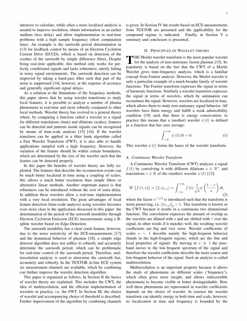
132.5 GHz135.5 GHz138.5 GHz141.5 GHz144.5 GHz147.5 GHz

Figure 2: Line-of-sight receiver data sampled at 100 kHz,TEXTOR discharge No. 106482. It shows a detailed viewaround 1.6 s, such that the periodic sawtooth behavior isvisible. The inversion radius, which is situated near the q = 1surface, just above channel 2 (135.5 GHz).

positive and negative effects. Consequently, measurement ofthe period is essential.

In this paper the sawtooth instability is studied by meansof in-line ECE-measurements in TEXTOR, which indirectlymeasures plasma temperatures [17]. This system is chosenbecause it is combined with Electron Cyclotron ResonanceHeating (ECRH), such that the sawtooth period can be alteredusing ECRH in the same line of sight if necessary. In Fig.2 such ECE-measurements in TEXTOR are shown. The saw-tooth period can be determined based on the crash [13], [14],however, due to the noise sensitivity of ECE-measurementsand the dynamical behavior of plasmas, a simple edge detectoralgorithm often does not suffice to robustly and accuratelydetermine the sawtooth period. In addition, if the sawtoothperiod needs to be controlled in real-time, the sawtooth perioddetection algorithm should also have a small delay. In theTEXTOR in-line ECE system six measurement channels areavailable, which can be combined to further improve thewavelet detection algorithm.

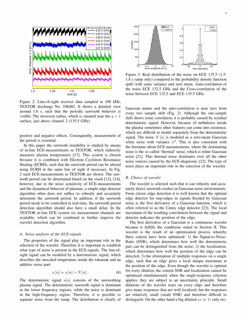
A. Noise analysis of the ECE-signals

The properties of the signal play an important role in theselection of the wavelet. Therefore it is important to establishwhat type of noise is present in the ECE-signals. The line-of-sight signal can be modeled by a deterministic signal, whichdescribes the unscaled temperature inside the tokamak and anadditive noise part:

x [n] = u [n] +N [n] . (8)

The deterministic signal u[n] consists of the sawtoothingplasma signal. The deterministic sawtooth signal is dominantin the lower frequency regions, while the noise is dominantin the high-frequency region. Therefore, it is possible toseparate noise from the ramp. The distribution is clearly of

−0.2 −0.1 0 0.1 0.20

500

1000

1500

2000

2500

noise amplitude [A.U.]

sam

ples

realgauss

−10 0 100

0.2

0.4

0.6

0.8

1

time [samples]

AutoCross

Figure 3: Real distribution of the noise on ECE 135.5 (1.5-1.8 s ramp only) compared to the probability density function(pdf) with same variance and zero mean. Auto-correlation ofthe noise ECE 132.5 GHz and the Cross-correlation of thenoise between ECE 132.5 and ECE 135.5 GHz.

Gaussian nature and the auto-correlation is near zero fromevery two sample shift (Fig. 3). Although the one-sampleshift shows some correlation, it is probably caused by residualdeterministic signal. However, because of turbulence insidethe plasma sometimes other features can come into existence,which are difficult to model separately from the deterministicsignal. The noise N [n] is modeled as a zero-mean Gaussianwhite noise with variance σ2. This is also consistent withthe literature about ECE-measurements, where the dominatingnoise is the so called ‘thermal’ noise, which is white Gaussiannoise [21]. This thermal noise dominates over all the othernoise sources caused by the ECE-diagnostic [22]. The type ofnoise plays an important role in the selection of the wavelet.

B. Choice of wavelet

The wavelet is selected such that it can robustly and accu-rately detect sawtooth crashes in Gaussian noise environments.From classic edge detection it is well known that the optimaledge detector for step-edges in signals flooded by Gaussiannoise is the first derivative of a Gaussian function, which isoften referred to as the Canny edge detector [23]. The localmaximum of the resulting convolution between the signal anddetector indicates the position of the edge.

The first derivative of a Gaussian is a continuous waveletbecause it fulfills the conditions stated in Section II. Thiswavelet is the result of an optimization process wherebythree criteria have been optimized: 1) the Signal-to-Noise-Ratio (SNR), which determines how well the deterministicpart can be distinguished from the noise; 2) the localization,which determines how well the position of the edge can bedetected; 3) the elimination of multiple responses on a singleedge, such that an edge gives a local unique maximum atthe position of the edge. Even though the wavelet is optimalfor every dilation, the criteria SNR and localization cannot beoptimized simultaneously when the single-response criterionapplies; they are subject to an uncertainty principle. Smalldilations of the wavelet react on every edge and thereforegive many responses that are well localized, but the responsesare relatively small (small SNR) and therefore difficult todistinguish. On the other hand a big dilation (s� 1) only rec-

5

1.59 1.60 1.61time [s]E

CE

cha

nnel

2 [A

.U.]

Scale of colors from MIN to MAX

Sca

les

[A.U

.]

1.59 1.60 1.61 1

8

16

24

32

40

48

56

64

Scale of colors from MIN to MAX

Sca

les

[A.U

.]

1.59 1.60 1.61 1

8

16

24

32

40

48

56

64

1.59 1.60 1.61EC

E c

hann

el 3

[A.U

.]

time [s]

Figure 4: Line-of-sight receiver data of noisy channel 2 (135.5GHz) and channel 3 (138.5 GHz) of TEXTOR discharge No.106482 measured around 1.6 s and their Continuous WaveletTransforms (contour plots) using the first derivative of theGaussian for scales s = 1 to s = 64.

ognizes big edges, however, the maximum is also influencedby events around the edge, making it difficult to determine thelocation of the edge. The key result is that when an edge isdetected in a big dilation, where it is clearly distinguishable, itsmaxima line is followed. This line, called a maxima chain, isfollowed until the well localized maxima at the position of theedge is found, i.e. sawtooth crashes can be well distinguishedand at the same time can be well localized. It has also beenshown to work well for points of sharp variations such asridges and other edges [24]. In Fig. 4, the contour plots of aCWT are shown, where vertical dark lines, which are wide ata big dilation and become narrower moving to small dilationsof the wavelet, reveal the sawtooth crashes. However, theselines do not end on s = 1 but somewhat above, which is aconsequence of noise and ridges being analyzed by a step edgedetector. This makes it impossible to find the middle of theedge in one point. Nevertheless, the position of the edge canbe well determined.

0 1 2 3 4

0.0625

0.25

0.375

0.5

n

Cubic B−spline

0 1

−0.5

−0.25

0

0.25

0.5

n

First Derivative B−spline

Figure 5: Cubic B-spline and its first time derivative, wherethe grey lines present the half-size B-splines used in (5) and(6)

C. Discrete implementation

The first derivative of a Gaussian is a continuous wavelet,which is not suitable to use in a FWT. A common method toapproximate a Gaussian function for this type of applicationis by using compactly supported B-splines, which fulfill (5)and (6) [24]. The B-spline βp (t), which serves as the scalingfunction φ (t), is constructed by repeated convolutions of thebox-spline. The scaling function converges with increasingorder p to a Gaussian (for odd p) [25]:

φ (t) = βp (t) =1p!

p+1∑q

(p+ 1q

)(−1)q

(t− q +

p+ 12

)p+

.

(9)The B-spline fulfills (5) for any s0 ∈ N [26]:

1s0βp(t

s0

)=

+∞∑n=−∞

bps0 [n]βp (t− n) , (10)

where Bps0 (z) respectively L (z) in terms of (5) is calculatedby:

L (z) = Bps0 (z) =1sp0

(s0−1∑n=0

z−n

)p+1

. (11)

The approximation order p and the dilation s0 can be chosendifferently for the application and consequently give extradesign freedom.

In this paper is chosen to use a cubic B-spline (p = 3) (Fig.5) because its approximation error is less than 3% compared toa Gaussian and it is within 2% of the limit of the Heisenberguncertainty [27]. The cubic B-spline is applied on a dyadicgrid (s0 = 2), which is a common choice. It has the advantagethat the calculated scales are relatively close together wherea maxima chain is difficult to follow and scales are far apart,where detection is important. The B-spline (9) needs to beinterpolated as described in (7) to determine Φ (z) such that thefirst scale gives generally useful maxima (symmetric functioni.e. Φ (z)=Φ

(z−1)). Another important property of B-splines

is that the difference of two shifted B-splines gives an evenbetter approximation (p+1) of the first derivative of a Gaussian[25]:

6

1.5015 1.502 1.5025 1.503 1.5035 1.504 1.5045 1.505 1.5055

0

0.5

1

1.5

2

2.5

3

time [s]

Wav

elet

coe

ffici

ents

SawtoothThresholdm=1m=2m=3m=4m=5m=6m=7rt det.

Figure 6: Real-time response of the wavelet coefficients on asawtooth measured on 132.5 GHz of discharge No. 106482,where a very robust threshold is chosen. The right pointingtriangle (red) is the point of detection, the other trianglespresent the selected maxima, where the last triangle (black)illustrates the chosen maxima. The vertical dash-dot lineshows the real-time instant of detection (rt det.). The waveletcoefficients for the different scales are the parabola shapedcurves from m = 1 (yellow) to m = 7 (black). The sawtoothhas been scaled for illustrational reasons.

ψ (t) =dβp+1 (t)

dt= βp (t)− βp (t− 1) . (12)

It can be rewritten similarly to (6) such that is is possible todefine h [n]:

ψ (t) =∞∑

n=−∞h [n]βp (t− n) , with h [n] = [1,−1] .

The resulting filters, which completely define the wavelettransform: L (z), H (z) and Φ (z) can also be found in TableI in the Appendix.

Remark 3: The second derivative of a Gaussian (a.k.a. theMexican hat wavelet) can be found using h [n] = [1,−2, 1][26]. Edges are detected by means of zero-crossings (Marr-Hildreth [28]) and is generally seen as equivalent to the firstderivative [23], [24]. �

D. Real-time sawtooth crash detection

Sawtooth crashes are detected when the wavelet coefficientsexceed a critical threshold value, which are calculated real-time resulting in delayed responses. This is shown in Fig. 6.Big dilations of the wavelet are delayed more compared tothat of the small dilations. In contrast, wavelet coefficientscalculated with small dilations often do not exceed a chosenthreshold, whereas for big dilations the coefficients exceedthe threshold (Section III-B). Therefore, a tight threshold issensitive to false detections, especially in scenarios with smallpartial reconnection events, but on the other hand the edgedetector has a small delay.

It is difficult to calculate the optimal threshold, however,it is possible to determine a lower-bound for the threshold.The minimum threshold should always be taken such thatit will not detect wavelet coefficients that are the result ofnoise. Therefore, an adaptive threshold is used such thata near optimal trade-off between robustness and delay canbe achieved. As explained in Section III-A the filter bankentrance noise is of Gaussian nature, which means that thewavelet coefficients resulting from this noise are also Gaussiandistributed [29]. The finiteness of the signal means that it ispossible to define a risk, in terms of the variance (σ2), ofdetecting noise. A well-known threshold from wavelet theoryof which the maximum noise amplitude has a very highprobability of being just below is [12]:

Tmin = σ√

2logeN. (13)

The lower bound threshold Tmin depends on the number ofsample points N , which is a logical consequence of the factthat if the number of points increase, the chance of takingpoints from the tail of the Gaussian distribution increases.

The variance of the noise in (13) on which the thresholdis based, needs to be calculated for every scale. This wouldmake the algorithm very inefficient. However, it is possible tomake an estimate of the variance for every scale based on the2-norm of one scale. Every branch of the filter bank can berepresented by one equivalent filter W [n], which is normalizedto one. This makes it possible to estimate an upperbound onthe noise in terms of the variance, which acts as the lowerbound on the threshold (Cauchy-Schwarz inequality):

|〈W,N〉| ≤ ‖W [n]‖2 ‖N [n]‖2 . (14)

The variance is estimated by the output of the first scale (d1),which mainly consists of noise. This has the advantage thatno additional calculation steps need to be taken to separate thenoise and allows for a bit more robust estimation because thesmall responses on sawteeth are included. Other possibilitiesare to estimate the signals noise by use of automatic varianceestimators, which are present in many signal processing soft-ware, which allows for a threshold purely based on noise butlacks robustness on dynamical behavior of the plasma.

The real threshold is always chosen above Tmin. However,this threshold is not robust due to the dynamical plasmabehavior. Therefore it needs to be chosen above Tmin (as amultiple of Tmin) . This is a good alternative because Fig. 6clearly shows there is still a significant margin above the realnoise level (≈ 0.2) to detect the sawtooth crash. It is evenpossible to add additional scales until a wavelet that has thesize of twice the period such that the response is even moresignificant and the region in which the threshold can be chosenis extended but at the cost of delay and calculation time.

The threshold is preferably chosen one-sided due to thefact that bigger wavelets also start responding on the ramp-part of the signal but in negative direction. For a two sidedthreshold this would lead to an over robustly threshold, whicheventually would lead to misses. In addition only maxima ofthe different wavelet scales on one side need to be determined

7

and stored. However, this makes a real-time estimate of theinversion radius necessary.

Summarizing, it is possible to estimate an absolute lower-bound on the threshold, however, it remains difficult to iden-tify an optimal threshold due to many different scenariosof sawtoothing plasmas. Consequently, to embed some extrarobustness, the wavelet coefficients of the first scale are usedas noise estimate, however, it is still necessary to take a higherthreshold.

E. Period determination

Sawtooth crashes can be detected robustly, however, it isstill necessary to accurately determine the location of thecrash and the resulting period. This is done by means of amaxima chain (Section III-B) whereby a number of maxima,which indicate the middle of the edge, are followed from themaxima in a scale m > 1 to lower scales preferably to m = 1.The maxima are detected in every scale by a simple maximadetector (d [1] < dmax [2] > d [3]) and are stored in a buffer,which has the size of the wavelet with the biggest dilation.Otherwise, due to the different delays for the different scales,important maxima can be lost.

Crashes are detected in scales m > 1. The wavelet co-efficients dm−1 are less delayed than dm, consequently it isgenerally possible to detect a sawtooth crash at scale m andselect the maximum at scale m−1, which belongs to the samecrash, this can be followed to the smallest crash (see Fig. 6).Great advantage is that at the time instant the sawtooth crashis detected, an accurate estimate of the position is calculated.

The non-causal responses (without delay) need to be cal-culated to be able to follow the maxima. This calculationis straightforward because the product of all filters in onebranch of the filter bank, which describe the wavelet, are anti-symmetric FIR-filters (linear-phase). Consequently the delayfor every scale is the length of the wavelet filter divided bytwo. The non-causal responses are shown in Fig. 7.

It is not always possible to follow the maxima chain to thesmallest scale m = 1 because sometimes there are more thanone or no maxima in the vicinity of the previous maxima. Con-sequently it is difficult to determine which maxima belongs tothe maxima of the detected edge. Therefore the maxima in thesmallest scale that can be traced back to the edge is selectedas the location of the crash, which could also be scale m− 1.The period is then calculated by taking the difference betweentwo consecutive crashes. In summary, the period determinationtakes place immediately after the detection and its resolutionis in principle independent of the detection scale. The maximachain allows a very accurate localization of the crash, hencealso of the period.

F. Combining channels

The line-of-sight ECE-system consists of six channels.Therefore it is possible to improve the wavelet algorithm bycombining the different channels. Not all channels are suitable:especially those near to the inversion radius often contain morenoise than signal, which can lead to loss of detection.

1.501 1.5015 1.502 1.5025 1.503 1.5035

0

0.5

1

1.5

2

2.5

3

time [s]

Wav

elet

coe

ffici

ents

SawtoothThresholdm=1m=2m=3m=4m=5m=6m=7rt det.

Figure 7: Non-causal response of the wavelet coefficients onthe same sawtooth (scaled) crash as presented in Fig. 6, whereclearly the maxima of the different scales are situated on aline, which leads to a good localization of the crash. The timeinstant of detection is represented by the dash-dot line (real-time detection) and as the right pointing triangle on scale m =6.

The responses of the wavelet coefficients on a crash for thedifferent channels on a scale m� 1 give significant responses,which are related to the amplitude and the sign of the sawteeth.This also holds for a channel near the inversion radius wherethe wavelet coefficients are too low to trigger a threshold, butstill give a distinguishable response compared to the noiselevel. The sign and amplitude of the wavelet coefficients onall channels at a crash indicate the location of the inversionradius, which can be estimated by finding the zero-crossing ofa function fitted through these wavelet coefficients (channelsneed to be calibrated).

The wavelet transform is performed parallel on channels 1-5. Channel 6 (147.5 GHz) is prone to non-linearity and cross-talk and has been gained extremely high [30]. Therefore, itcannot be trusted; this channel is not used in the algorithm. Itis possible by comparing the channels 1-5 to suppress thesefalse crashes, because often a false crash only occurs on onechannel. Therefore, an evaluation block has been designed,which observes real-time the crash time instants, if enoughcrashes (here 2) from the different channels have been detectednear the same location, the mean is taken. Together with theprevious crash, the difference is calculated resulting in theperiod. The next detection events are blocked for some periodafter the detection. If during a certain observation time onlyone (false) crash is detected, the specific channel is reset.

IV. RESULTS

BASIC sawteeth, as presented in Fig. 7, do not poseany problem for this type of algorithm. However, there

is a variety of sawteeth that are much more difficult todetect, whereof some are discussed here. The sawteeth are allextracted from Channel 1 (132.5 GHz) of TEXTOR discharges

8

1.601 1.6015 1.602 1.6025 1.603 1.6035 1.604

0

0.5

1

1.5

2

2.5

3

time [s]

Wav

elet

coe

ffici

ents

SawtoothThresholdm=1m=2m=3m=4m=5m=6m=7rt det.

Figure 8: Non-causal response on bump, where the rightpointing triangle is the point of detection and the dash-dotline the real-time location of detection (rt det.). (132.5 GHz,discharge No. 106482, robust threshold)

No. 106482 and No. 107915. The responses are calculated bya detection algorithm, which is implemented in a real-timetesting environment (Simulinkr). The chosen parameters arefound in Table of the Appendix II. In addition to the sawteeth,also the period is calculated in a real-time environment, for theindividual channels and for the combination of channels.

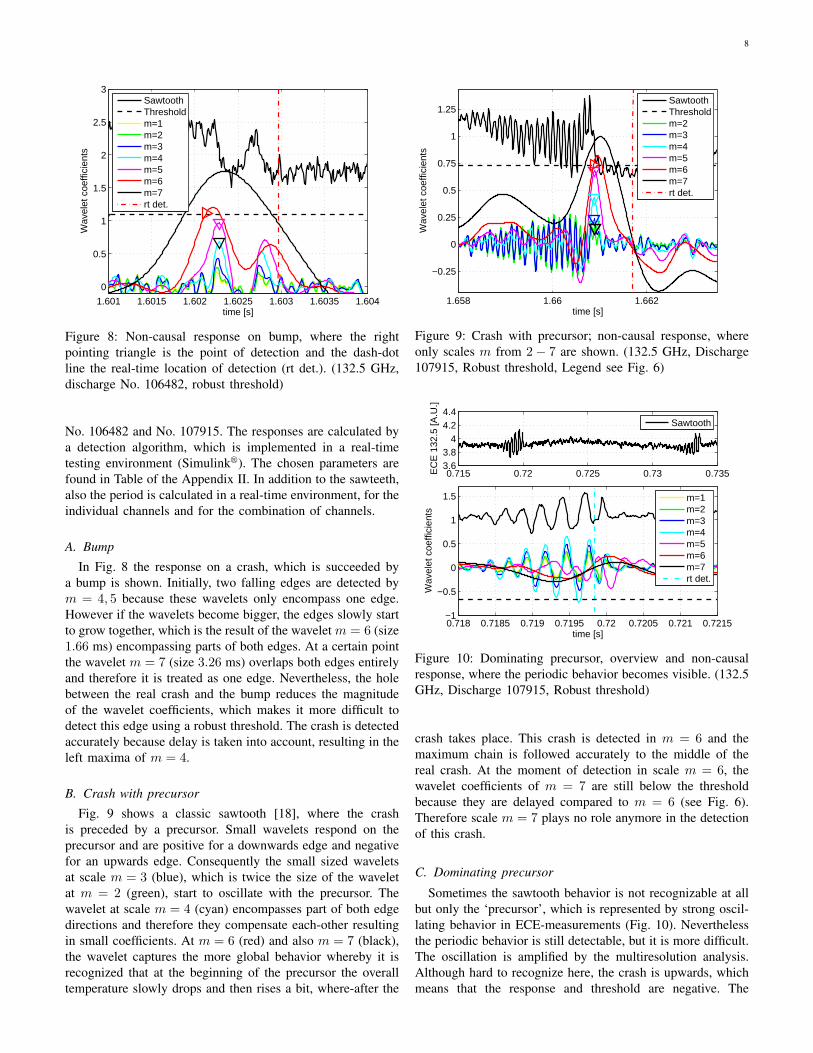
A. Bump

In Fig. 8 the response on a crash, which is succeeded bya bump is shown. Initially, two falling edges are detected bym = 4, 5 because these wavelets only encompass one edge.However if the wavelets become bigger, the edges slowly startto grow together, which is the result of the wavelet m = 6 (size1.66 ms) encompassing parts of both edges. At a certain pointthe wavelet m = 7 (size 3.26 ms) overlaps both edges entirelyand therefore it is treated as one edge. Nevertheless, the holebetween the real crash and the bump reduces the magnitudeof the wavelet coefficients, which makes it more difficult todetect this edge using a robust threshold. The crash is detectedaccurately because delay is taken into account, resulting in theleft maxima of m = 4.

B. Crash with precursor

Fig. 9 shows a classic sawtooth [18], where the crashis preceded by a precursor. Small wavelets respond on theprecursor and are positive for a downwards edge and negativefor an upwards edge. Consequently the small sized waveletsat scale m = 3 (blue), which is twice the size of the waveletat m = 2 (green), start to oscillate with the precursor. Thewavelet at scale m = 4 (cyan) encompasses part of both edgedirections and therefore they compensate each-other resultingin small coefficients. At m = 6 (red) and also m = 7 (black),the wavelet captures the more global behavior whereby it isrecognized that at the beginning of the precursor the overalltemperature slowly drops and then rises a bit, where-after the

1.658 1.66 1.662

−0.25

0

0.25

0.5

0.75

1

1.25

time [s]

Wav

elet

coe

ffici

ents

SawtoothThresholdm=2m=3m=4m=5m=6m=7rt det.

Figure 9: Crash with precursor; non-causal response, whereonly scales m from 2− 7 are shown. (132.5 GHz, Discharge107915, Robust threshold, Legend see Fig. 6)

0.715 0.72 0.725 0.73 0.7353.63.8

44.24.4

EC

E 1

32.5

[A.U

.]

0.718 0.7185 0.719 0.7195 0.72 0.7205 0.721 0.7215−1

−0.5

0

0.5

1

1.5

time [s]

Wav

elet

coe

ffici

ents

Sawtooth

m=1m=2m=3m=4m=5m=6m=7rt det.

Figure 10: Dominating precursor, overview and non-causalresponse, where the periodic behavior becomes visible. (132.5GHz, Discharge 107915, Robust threshold)

crash takes place. This crash is detected in m = 6 and themaximum chain is followed accurately to the middle of thereal crash. At the moment of detection in scale m = 6, thewavelet coefficients of m = 7 are still below the thresholdbecause they are delayed compared to m = 6 (see Fig. 6).Therefore scale m = 7 plays no role anymore in the detectionof this crash.

C. Dominating precursor

Sometimes the sawtooth behavior is not recognizable at allbut only the ‘precursor’, which is represented by strong oscil-lating behavior in ECE-measurements (Fig. 10). Neverthelessthe periodic behavior is still detectable, but it is more difficult.The oscillation is amplified by the multiresolution analysis.Although hard to recognize here, the crash is upwards, whichmeans that the response and threshold are negative. The

9

1.61 1.615 1.62 1.625 1.63 1.635 1.64 1.645−2

−1.5

−1

−0.5

0

0.5

1

1.5

2

2.5

3

3.5

time [s]

Wav

elet

coe

ffici

ents

m=3m=6m=9rt det.

Figure 11: Near detection failure, in a regime with well definedsawteeth, due to a number of reasons. (132.5 GHz, dischargeNo. 107915, robust threshold)

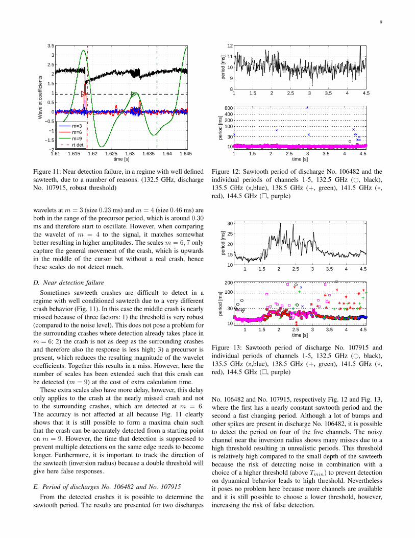
wavelets at m = 3 (size 0.23 ms) and m = 4 (size 0.46 ms) areboth in the range of the precursor period, which is around 0.30ms and therefore start to oscillate. However, when comparingthe wavelet of m = 4 to the signal, it matches somewhatbetter resulting in higher amplitudes. The scales m = 6, 7 onlycapture the general movement of the crash, which is upwardsin the middle of the cursor but without a real crash, hencethese scales do not detect much.

D. Near detection failureSometimes sawteeth crashes are difficult to detect in a

regime with well conditioned sawteeth due to a very differentcrash behavior (Fig. 11). In this case the middle crash is nearlymissed because of three factors: 1) the threshold is very robust(compared to the noise level). This does not pose a problem forthe surrounding crashes where detection already takes place inm = 6; 2) the crash is not as deep as the surrounding crashesand therefore also the response is less high; 3) a precursor ispresent, which reduces the resulting magnitude of the waveletcoefficients. Together this results in a miss. However, here thenumber of scales has been extended such that this crash canbe detected (m = 9) at the cost of extra calculation time.

These extra scales also have more delay, however, this delayonly applies to the crash at the nearly missed crash and notto the surrounding crashes, which are detected at m = 6.The accuracy is not affected at all because Fig. 11 clearlyshows that it is still possible to form a maxima chain suchthat the crash can be accurately detected from a starting pointon m = 9. However, the time that detection is suppressed toprevent multiple detections on the same edge needs to becomelonger. Furthermore, it is important to track the direction ofthe sawteeth (inversion radius) because a double threshold willgive here false responses.

E. Period of discharges No. 106482 and No. 107915From the detected crashes it is possible to determine the

sawtooth period. The results are presented for two discharges

1 1.5 2 2.5 3 3.5 4 4.58

9

10

11

12

perio

d [m

s]

1 1.5 2 2.5 3 3.5 4 4.510

30

100200400800

time [s]

perio

d [m

s]

Figure 12: Sawtooth period of discharge No. 106482 and theindividual periods of channels 1-5, 132.5 GHz (#, black),135.5 GHz (x,blue), 138.5 GHz (+, green), 141.5 GHz (∗,red), 144.5 GHz (�, purple)

1 1.5 2 2.5 3 3.5 4 4.510

15

20

25

30pe

riod

[ms]

1 1.5 2 2.5 3 3.5 4 4.510

30

100

200

time [s]

perio

d [m

s]

Figure 13: Sawtooth period of discharge No. 107915 andindividual periods of channels 1-5, 132.5 GHz (#, black),135.5 GHz (x,blue), 138.5 GHz (+, green), 141.5 GHz (∗,red), 144.5 GHz (�, purple)

No. 106482 and No. 107915, respectively Fig. 12 and Fig. 13,where the first has a nearly constant sawtooth period and thesecond a fast changing period. Although a lot of bumps andother spikes are present in discharge No. 106482, it is possibleto detect the period on four of the five channels. The noisychannel near the inversion radius shows many misses due to ahigh threshold resulting in unrealistic periods. This thresholdis relatively high compared to the small depth of the sawteethbecause the risk of detecting noise in combination with achoice of a higher threshold (above Tmin) to prevent detectionon dynamical behavior leads to high threshold. Neverthelessit poses no problem here because more channels are availableand it is still possible to choose a lower threshold, however,increasing the risk of false detection.

10

2.5 2.6 2.7 2.8 2.9

1

2

3

4

5

6

time [s]

EC

E c

hann

els

1−5

[A.U

.]

ec132ec135ec138ec141ec144T

crash

Figure 14: Sawteeth of discharge No. 107915, where • rep-resent detection on the individual channels and the lines theposition of the crash. The crashes are missed during the changeof inversion radius.

The period of discharge No. 107915 is more difficult tomeasure due to a lot of dynamical behavior, which is notfully understood and an inversion radius that moves throughchannels, which is represented in Fig. 14. False detectionsrarely occur due to a robust threshold, however resulting inerrors, which are predominately made by misses. This can betaken care of by combining channels to determine robustlythe sawtooth period. From this discharge the great advantageof the wavelet based algorithm becomes clear because itis possible to identify the individual periods, whereas thefrequency based methods will give an averaged period.

F. Compound regime

The real-time wavelet detection algorithm due to mul-tiresolution can distinguish small intermediate crashes frombigger real crashes (see Fig. 15). The smaller wavelets upto scale m = 7 react strongly on the intermediate crashesat 2.48 s and 2.518 s as if it are normal crashes. However,if the scales become bigger, the magnitude of the waveletcoefficients become smaller again, where m = 8 still detectsthe intermediate crashes but its magnitude is smaller than theprevious scale m = 7. At scale m = 9 the intermediate crashesstarts to disappear, whereas the magnitude for the real crashesat 2.47 s, 2.49 s and 2.51 s have become bigger (but delayed).Although in m = 9 the wavelet coefficients are negative atthe intermediate crashes, it is still recognizable by the upwardmovement that an intermediate crash is present. Consequently(in principle), multiresolution analysis can differentiate be-tween intermediate crashes and real crashes, which allowsidentification of compound regimes.

G. Accuracy

It is generally not possible to give a real estimate of the errorbecause the real period is unknown. However, it is possible fora regime with well defined sawtooth crashes to compare the

2.45 2.46 2.47 2.48 2.49 2.5 2.51 2.52 2.53

−2

−1

0

1

2

3

4

time [s]

Wav

elet

coe

ffici

ents

m=6 m=7 m=8 m=9 rt det.

Figure 15: Sawteeth with intermediate crashes, where thewavelet at m = 8 feels the small crash less and m = 9 not atall (non-causal).

1 1.2 1.4 1.6 1.8 29

9.5

10

10.5

11

11.5

12

12.5

time [s]

perio

d [m

s]

period ECE 132.5 GHzperiod ECE 138.5 GHzperiod

Figure 16: Period estimates of two individual channels com-pared to the the period estimate of discharge No. 106482

calculated period to the individual estimates of the period. Thisis presented in Fig. 16. The uncertainty of the period fluctu-ates much more than the difference between the individualchannels, which are generally close to each other. This alsofollows from the standard deviations, measured from 1− 4 s,where the standard deviation of the period is σperiod = 0.51ms and respectively of the differences: σ132.5−138.5 = 0.13ms, σ132.5−141.5 = 0.22 ms, and σ138.5−141.5 = 0.20 ms.Therefore it can be concluded that the error on the periodestimates of the individual channels is much smaller than thatof the uncertainty of the period itself. The two signals withthe best SNR (ECE 132.5 and 138.5 (see Fig. 2)) give the bestestimates, the difference between the best estimates comparedto the uncertainty is almost 4 times higher, consequently itis not useful for general sawteeth to further improve thealgorithm with respect to the accuracy.

11

V. SUMMARY AND CONCLUSIONS

AN algorithm for accurate real-time detection of sawtoothcrashes has been developed. The algorithm is based

on time-scale wavelet theory and edge-detection. The perfor-mance of the algorithm is tested and compared with othermethods, such as the single band pass-filter. Detection of ‘stan-dard’ sawtooth crashes was demonstrated to have considerablyless delay than a single band-pass filter, which needs to detectall crashes accurately. It is also shown that more challengingsawteeth crashes can be handled, as a consequence of therobust scales. The choice of a general edge detector instead ofan optimized sawtooth detector is justified by the existence ofmany different types of sawteeth and the realized accuracy ofthe detection algorithm, which is well below the uncertaintyof the sawtooth period itself for most crashes. Moreover,multiresolution enables distinction between different sizes ofsawtooth crashes due to the different sizes of wavelets.

Tests show that a flawless period estimation algorithm basedon edge detection due to the dynamical behavior of the plasmais not possible. This complicates the selection of an optimalthreshold. Nevertheless, the algorithm simplifies the selectionof a proper threshold as a consequence of the better SNRof wavelet scales (m � 1) (band-pass filters) compared tothe single band-pass filter based algorithms presented in [14],[13]. Further improvements of the algorithm are possible bycombining ECE-channels.

Therefore, the current algorithm is the intermediate step forperiod estimation between a very robust detection algorithmbased on the Morlet Wavelet, which is difficult to implementin real-time and the current real-time implemented simple oneband-pass filter methods. Due to the calculation of at leasttwo scales, the algorithm allows an immediate and accurateestimate of the crash position in time. Numerically, the pro-posed algorithm has a high flexibility e.g. the step size s0 inscales s can be varied due to the B-spline implementation,and the initial scale can be chosen by varying the pre-filter. Inaddition, the wavelets are calculated with a filter bank, whichfilters are (anti-)symmetric and contain only a few non-zerocoefficients, which makes the implementation very efficientand consequently real-time applicable as demonstrated in aSimulinkr implementation.

APPENDIX

The filter coefficients used are given in Table I, the otherparameters are given in Table II.

REFERENCES

[1] J. Bizarro and A. Figueiredo, “Time–frequency analysis of fusionplasma signals beyond the short-time Fourier transform paradigm: Anoverview,” Fusion Engineering and Design, vol. 83, no. 2-3, pp. 350–353, 2008.

[2] S. Santoso, E. Powers, R. Bengtson, and A. Ouroua, “Time-seriesanalysis of nonstationary plasma fluctuations using wavelet transforms,”Review of Scientific Instruments, vol. 68, p. 898, 1997.

[3] K. Hallatschek and M. Zilker, “Real time data acquisition with transput-ers and PowerPCs using thewavelet transform for event detection,” IEEETransactions on Nuclear Science, vol. 45, no. 4 Part 1, pp. 1872–1876,1998.

Table I: Filter coefficients that generate the cubic B-splinescaling functions and its derivative.

n L (z) L(z2)

Φ0 (z) H (z)

0 0.0625 0.0625 0.0029 -0.51 0.2500 0 0.0234 0.52 0.3750 0.2500 0.07863 0.2500 0 0.16374 0.0625 0.3750 0.23145 0 0.23146 0.2500 0.16377 0 0.07868 0.0625 0.02349 0.0029

Table II: Parameters used to generate figures

Parameter ValueC 3

Increase threshold based on noise m = 1 by factorChannels 2

Number of channels in which crash is detected such that it is forwardedBlock Time 2.43 ms

Time detection is blocked after crash: maximum delay 1.63 ms + 0.2 msDistance between maxima [2 2 2 2 2 5 5 5]

Maximum distance between maxima; if bigger, chain is brokenBuffer size 2.23 ms

Storage of maxima in a matrix [Boolean]Delay 0.08, 0.13, 0.23, 0.43, 0.83, 1.63 ms

Delay of detection compared to the crash time (m = 8, 93.23, 6.43 ms)

[4] A. Figueiredo, M. Nave, and J. Contributors, “Time-frequency analysisof nonstationary fusion plasma signals: A comparison between the Choi-Williams distribution and wavelets,” Review of Scientific Instruments,vol. 75, no. 10, pp. 4268–4270, 2004.

[5] F. Poli, S. Sharapov, and S. Chapman, “Study of the spectral properties ofELM precursors by means of wavelets,” Plasma Physics and ControlledFusion, vol. 50, p. 095009, 2008.

[6] T. Kass, S. Gunter, M. Maraschek, W. Suttrop, H. Zohm, and A. Team,“Characteristics of type I and type III ELM precursors in ASDEXupgrade,” Nuclear Fusion, vol. 38, no. 1, pp. 111–116, 1998.

[7] J. Stober, M. Maraschek, G. Conway, O. Gruber, A. Herrmann, A. Sips,W. Treutterer, and H. Zohm, “Type II ELMy H modes on ASDEXUpgrade with good confinement at high density,” Nuclear Fusion,vol. 41, pp. 1123–1134, 2001.

[8] M. Nave, E. Lazzaro, R. Coelho, P. Belo, D. Borba, R. Buttery,S. Nowak, F. Serra, and E. Contributors, “Triggering of neo-classicaltearing modes by mode coupling,” Nuclear Fusion, vol. 43, no. 3, pp.179–187, 2003.

[9] B. P. van Milligen, C. Hidalgo, and E. Sánchez, “Nonlinear phenomenaand intermittency in plasma turbulence,” Phys. Rev. Lett., vol. 74, no. 3,pp. 395–398, Jan 1995.

[10] M. Heller, Z. Brasilio, I. Caldas, J. Stöckel, and J. Petrzilka, “Scrape-offlayer intermittency in the Castor tokamak,” Physics of Plasmas, vol. 6,p. 846, 1999.

[11] J. Bizarro and A. Figueiredo, “The Wigner distribution as a tool for time-frequency analysis of fusion plasma signals: application to broadbandreflectometry data,” Nuclear Fusion, vol. 39, pp. 61–82, 1999.

[12] S. Mallat, A wavelet tour of signal processing; The sparse way, 3rd ed.Academic Press, London, 2009.

[13] M. Lennholm and L. Eriksson, “Closed Loop Sawtooth Period ControlUsing Variable Eccd Injection Angles On Tore Supra,” Fusion Scienceand Technology, vol. 55, no. 1, pp. 45–55, 2009.

[14] J. Paley, F. Felici, S. Coda, T. Goodman, and F. Piras, “Real timecontrol of the sawtooth period using EC launchers,” Plasma Physicsand Controlled Fusion, vol. 51, p. 055010, 2009.

[15] P. S. Addison, The illustrated wavelet transform handbook : introductorytheory and applications in science, engineering, medicine and finance,S. Laurenson, Ed. Institute of Physics, Bristol, 2002.

[16] C. S. Burrus, R. A. Gopinath, and H. Guo, Introduction to Wavelets andWavelet Transforms, A primer, M. Horton, Ed. Prentice Hall, UpperSaddle River, New Jersey 07458, 1998.

[17] J. Oosterbeek, A. Bürger, E. Westerhof, M. De Baar, M. Van Den Berg,

12

W. Bongers, M. Graswinckel, B. Hennen, O. Kruijt, J. Thoen et al.,“A line-of-sight electron cyclotron emission receiver for electron cy-clotron resonance heating feedback control of tearing modes,” Reviewof Scientific Instruments, vol. 79, p. 093503, 2008.

[18] R. Hastie, “Sawtooth instability in tokamak plasmas,” Astrophysics andSpace Science, vol. 256, no. 1, pp. 177–204, 1997.

[19] A. Calderon, “Intermediate spaces and interpolation, the complexmethod,” Studia Math, vol. 24, no. 2, pp. 113–190, 1964.

[20] I. Daubechies, Ten Lectures on Wavelets. Siam publications, Philadel-phia, 1992, vol. 61 CMBMS-NSF Series in Applied Mathematics.

[21] H. Hartfuss, T. Geist, and M. Hirsch, “Heterodyne methods in millimetrewave plasma diagnostics with applications to ECE, interferometry andreflectometry,” Plasma Physics and Controlled Fusion, vol. 39, pp.1693–1769, 1997.

[22] I. Classen, L. Cardozo, F. Schüller, R. Jaspers et al., “Imaging andcontrol of magnetic islands in tokamaks,” 2007.

[23] J. Canny, “A Computational Approach to Edge Detection,” Readings incomputer vision: issues, problems, principles, and paradigms, p. 184,1987.

[24] S. Mallat and S. Zhong, “Characterization of signals from multiscaleedges,” IEEE Transactions on pattern analysis and machine intelligence,vol. 14, no. 7, pp. 710–732, 1992.

[25] M. Unser, “Splines: A perfect fit for signal and image processing,” IEEESignal processing magazine, vol. 16, no. 6, pp. 22–38, 1999.

[26] Y. Wang and S. Lee, “Scale-space derived from B-splines,” IEEETransactions on Pattern Analysis and Machine Intelligence, vol. 20,no. 10, pp. 1040–1055, 1998.

[27] M. Unser, “Ten good reasons for using spline wavelets,” vol. 3169, pp.422–431, 1997.

[28] D. Marr and E. Hildreth, “Theory of edge detection,” Proceedings of theRoyal Society of London. Series B, Biological Sciences, pp. 187–217,1980.

[29] G. Lebanon. (2006, 01) LTI Filtering of WSS Processes. Collegeof Computing (CSE), Georgia Institute of Technology. Viewed on2010-05. [Online]. Available: http://www.cc.gatech.edu/ lebanon/notes/

[30] J. Oosterbeek, “Towards a self-aiming microwave antenna to stabilisefusion plasmas,” Ph.D. dissertation, Technische Universiteit Eindhoven,2009.

Future Research

The edge detector (wavelet) can be further optimized to increase the magnitude of the result-ing wavelet coefficients, making it somewhat easier to detect (and in an earlier stadium) thesawtooth crashes. Although optimization of the wavelets to improve accuracy of the algorithmis not necessary.The threshold remains the Achilles’ heel of the algorithm, therefore it is important to fur-ther investigate a suitable threshold for individual situations. Another option is to make thethreshold choice less sensitive by for instance taking the square of the wavelet coefficients.The algorithm is preferably implemented on a FPGA when used real-time. Especially thenumber of scales should be chosen with care. In the case that still extra calculation power isnecessary it is also possible to add downsampling into the current algorithm but at the cost ofdelay.The combination of channels needs to be further improved. An alternative is to observe allcrashes from the different channels and decide on basis of an intelligent algorithm comparingheight and time instant of the crash, if it belongs to the period of the sawtooth signal. Fur-thermore noise needs to be further reduced by cross-correlating the different signals due to theuncorrelation of the noise between different channels but at the cost of some delay.Currently the direction of the sawteeth is based on the maxima and minima (observed in awindow) of the response on a crash, this generally works well because the crash gives a cleardirectional difference. However, the threshold is preferably based on the sign of the sawteethdue to the negative response of the wavelet coefficients from big wavelets. Therefore, especiallyin regimes where the inversion radius changes position between channels within a few periods,it is difficult to track. Consequently, making it difficult to track the sign of the sawtooth andfind a threshold in the right direction. Although for small wavelets the threshold can be takentwo-sided. Therefore it is important to develop an algorithm that tracks the inversion radiusreal-time independently from the crashes.

13

Appendices

Appendix A

Fast Wavelet Transform in thefrequency domain

A.1 Properties of the Fourier Transform

The following properties of the Fourier Transform are used:

f (at) =1|a| f

(ωa

)(A.1)

f(x− a) = e−iaω f(ω) (A.2)

dnf(x)dxn

= (iω)nf(ω) (A.3)

(f ∗ g)(x) = f(ω)g(ω) (A.4)

A.2 Wavelet and scaling functions time domain

The wavelet transform and scaling function with s0 = 2 are defined as:

dm [n] = 〈f, ψm,n〉 =ˆ +∞

−∞f (t) s−m/2

0 ψ(s−m0 t− n

)dt. (A.5)

am [n] = 〈f, φm,n〉 =ˆ +∞

−∞f (t) s−m/2

0 φ(s−m0 t− n

)dt. (A.6)

The DWT can be implemented in a Fast Wavelet Transform (FWT) if the scaling function hasthe following two properties: φ (t) can be written as a summation of different translations ofφm

(t2

), and ψ

(t2

)can be written as a summation of different translations of φ (t):

φ

(t

2

)=√

2∞∑

=−∞l [−n]φ (t− n) and, (A.7)

ψ

(t

2

)=√

2∞∑

n=−∞h [−n]φ (t− n) , (A.8)

17

18 Appendix A. Fast Wavelet Transform in the frequency domain

A.3 Wavelet and scaling functions in frequency domainThe Fourier transform of (A.5) and (A.6) are calculated with (B.1) and (A.4):

dm = 2m/2f (ω) ψ (2mω) , and (A.9)

am = 2m/2f (ω) φ (2mω) (A.10)

The Fourier transforms of (A.7) and (A.8) are given by (see also Appendix C [1]):

φ (2ω) =1√2L (ω) φ (ω) (A.11)

ψ (2ω) =1√2H (ω) φ (ω) (A.12)

It becomes clear that L (ω) describes the transfer from φ (ω) to φ (2ω).

A.4 Fast Wavelet Transform in frequency domainNow, all the tools to construct a fast wavelet transform in the frequency domain are available.For instance we wish to calculate the wavelet coefficients on scale m = 3, therefore (A.9) needsto be changed:

d3 = 2√

2ψ (8ω) f (ω) (A.13)

which, can be rewritten using (A.10) and (A.9) in a different form:

φ (4ω) = 2−0.5L (2ω) φ (2ω) , (A.14)

ψ (8ω) = 2−0.5H (4ω) φ (4ω) . (A.15)

Filling this into (A.13) we find:

d3 = 2 ·H (4ω) φ (4ω) f (ω) =√

2 ·H (4ω)L (2ω) φ (2ω) f (ω) , (A.16)

together with (A.14):

d3 = H (4ω)L (2ω)L (ω) φ (ω) f (ω) . (A.17)

Let’s compare this to that of m = 2:

d2 = H (2ω)L (ω) φ (ω) f (ω) . (A.18)

In addition the scaling coefficients a0, a1 and a2 are defined as:

a0 = f (ω) φ (ω) , a1 =√

2 · f (ω) φ (2ω) , and

a2 = 2 · f (ω) φ (4ω) , (A.19)

which is also equal to:

a1 = L (ω) φ (ω) f (ω) = L (ω) a0 (A.20)

Now, in combination with H (ω) it is possible to calculate from the scaling coefficients thewavelet coefficients.

d1 = H (ω)L (ω) a0. (A.21)

A.5. Samples as scaling coefficients 19

Consequently every wavelet coefficient can be calculated by a cascade of filters L (2mω) andH (ω) and starting scaling coefficients a0 = f (ω) φ (ω), which is better known as the FilterBank. However, these are often expressed in terms of z = ejω and therefore need to berewritten. Important to note is that l [−n] and h [−n] in (A.7) and (A.8) are already exactin z, as a consequence all calculated wavelet coefficients are exact, if we are dealing withcontinuous f (t). However, the signal is always discrete and thus the product a0 = f (ω) φ (ω)needs to be approximated, which has following form in the time domain:

a0 [n] = 〈f, φ0,n〉 ≈∞∑

k=−∞

f [k]φ0 [k − n] ,

thus introducing an error, dependent on the product. The increasing order has than followingform:

d3 (z) = H(z4)L(z2)L (z) φ

(z−1)F (z) .

A.5 Samples as scaling coefficientsIn the field of wavelet theory it is common practice to fill into the filter bank directly the signalinstead of the scaling coefficients, which is purely theoretical wrong as we have seen in theprevious section and leads to errors. However, this is only half-true because there is a secondmechanism, which partly justifies this choice: this is the convergence of the cascade L (2ω)L (ω)to the function φ (aω). This is explained in more detail in Section 6.5 and appendix C of [1],the convolution is defined in the frequency domain as (no normalization factors consideredanymore):

φ (ω) =∞∏

p=1

L( ω

2p

).

Let’s for instance consider a4, which can be calculated by:

a4 = f (ω) φ (16ω) = L (8ω)L (4ω)L (2ω)L (ω) φ (ω) f (ω) .

This means that φ (16ω) is approximately:

φ (16ω) =∞∏

p=1

L

(16ω2p

)≈ L (8ω)L (4ω)L (2ω)L (ω) .

Consequently the term φ (ω) becomes of less importance and justifies the choice of filling indirectly the signal samples. However, in the scales where m is still small the approximationis bad and consequently a big error is introduced, which becomes smaller with increasing m.Therefore the convergence rate of the cascade to φ is another important field of study.

Appendix B

Inversion radius

B.1 Theoretical background

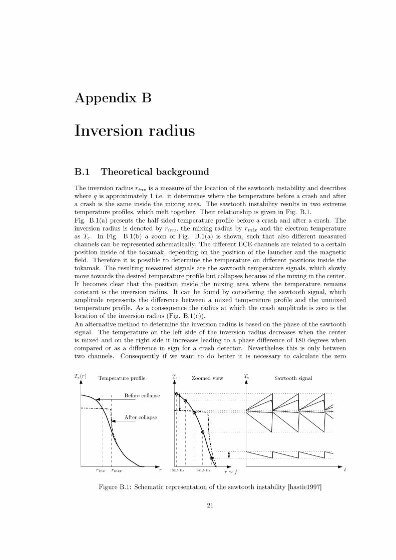
The inversion radius rinv is a measure of the location of the sawtooth instability and describeswhere q is approximately 1 i.e. it determines where the temperature before a crash and aftera crash is the same inside the mixing area. The sawtooth instability results in two extremetemperature profiles, which melt together. Their relationship is given in Fig. B.1.Fig. B.1(a) presents the half-sided temperature profile before a crash and after a crash. Theinversion radius is denoted by rinv, the mixing radius by rmix and the electron temperatureas Te. In Fig. B.1(b) a zoom of Fig. B.1(a) is shown, such that also different measuredchannels can be represented schematically. The different ECE-channels are related to a certainposition inside of the tokamak, depending on the position of the launcher and the magneticfield. Therefore it is possible to determine the temperature on different positions inside thetokamak. The resulting measured signals are the sawtooth temperature signals, which slowlymove towards the desired temperature profile but collapses because of the mixing in the center.It becomes clear that the position inside the mixing area where the temperature remainsconstant is the inversion radius. It can be found by considering the sawtooth signal, whichamplitude represents the difference between a mixed temperature profile and the unmixedtemperature profile. As a consequence the radius at which the crash amplitude is zero is thelocation of the inversion radius (Fig. B.1(c)).An alternative method to determine the inversion radius is based on the phase of the sawtoothsignal. The temperature on the left side of the inversion radius decreases when the centeris mixed and on the right side it increases leading to a phase difference of 180 degrees whencompared or as a difference in sign for a crash detector. Nevertheless this is only betweentwo channels. Consequently if we want to do better it is necessary to calculate the zero

Te(r)

r t

Te

Before collapse

After collapse

rinv rmix

Te Zoomed viewTemperature profile Sawtooth signal

r ∼ f132,5 Hz 141,5 Hz

Figure B.1: Schematic representation of the sawtooth instability [hastie1997]

21

22 Appendix B. Inversion radius

Figure B.2: Shot 107785 ECE output, shot 107786 Thomson scattering at 1.2 s [2]

of the function that describes the difference between the mixed temperature profile and theunmixed temperature profile. This can only be determined when the real difference in termsof temperature is known.

B.2 Temperature estimation

The real-time in-line Electron-Cyclotron-Emission-measurements on TEXTOR are all un-scaled. This means that the output voltage of the different channels needs to be related to thetemperature. For every channel this relationship needs to be determined individually. There-fore it is necessary that we know the DC Gain, which determines what the gain relationshipis between temperature and voltage. This is called the sensitivity

([eV ][V ]

). In addition we need

to know an initial value. Generally the temperature is determined using Thomson scattering,which needs to be performed prior to the experiment to be able to use it for real-time inversionradius estimation. However under the same conditions the relationship between voltage andtemperature remains similar, making it possible to perform this measurement in one of theshots prior to the experiment. This is explained in [2], which also presents an example ofThomson scattering (Fig. B.2)Using Thomson scattering it is possible to calculate the real temperature output. However,we are only interested in the amplitude of the sawtooth signal. Therefore it suffices to onlydetermine the sensitivity. This can be done as follows: First determine the initial DC gain(t =0 s), which corresponds to a very low temperature of about 0.025 eV and thus can beneglected. The voltage at 1.2 seconds is determined by the Thomson scattering, which enablesus to calculate the sensitivity as follows:Sens = Tthomson−T0

Vthomson,time−V0, consequently because we have the full shot including the heating

phase, we only need the temperature at one point inside the tokamak.

B.3 Estimate temperature without Thomson scattering

Sometimes we do not have a Thomson scattering measurement available. In that case weneed to make an estimate of the temperature based on the known variables. We will needthe following variables: the toroidal magnetic field strength BT ; the launcher angle and theshafronov shift Sshift. The magnetic field determines the relationship between frequency andthe radius. This is also dependent on the angle of the launcher. The inverse big radius dependson the ECER = ECEfrequency ·( 0.0102

BT). If the relationship between the channels and the radius

is determined, it is possible by estimating a temperature profile, to calculate the temperaturesof every channel. However, to estimate the temperature exactly it is necessary to compensatefor the Shafronov shift, which determines how much the temperature profile is shifted from

B.4. Example calculation Sensitivity (Shot 106478) 23

Table B.1: Required parameters

Parameter Symbol ValueBeta torodial BT 2.4 TLauncher angle Angle 0◦

Shafronov shift Sshift 1.81 cmTemperature center (estimate) T0 2200 eVTemperature wall (estimate) Ta 100 eV

Radius a 0.46 m

0 1 2 3 4 5

x 105

1

2

3

4

5

6

7

time [samples]

T [u

nsca

led]

Shot 106478

ec132ec135ec138ec141ec144

0 500 1000 1500 2000 2500 3000 3500 4000

0.6

0.8

1

1.2

1.4

1.6

1.8

time [samples]

T [u

nsca

led]

Shot 106478

ec132ec135ec138ec141ec144

Figure B.3: Unscaled temperature overview and start of Shot 106478

the center of the tokamak. This Shafronov shift is difficult to determine when the radius isdifferent from zero. Also the radius of the tokamak needs to be known (textor a = 0.46), thecenter and edge temperature needs to be valued (T0, Ta). The temperature profile can now beestimated by considering following approximation:

T = Ta + (T0 − Ta)

(1−

(Sshift (r)− r

a

)2)2

(B.1)

Now we have an estimate of the temperature, which belongs to the temperature profile justbefore the collapse. This makes it possible to make a rough estimate of the relationship betweenthe different amplitudes of our saw teeth by choosing a point at the top of the temperature.Although this estimate is rough due to the big difference between the temperature at the startof the experiment and the desired temperature, which results in a sensitivity near enough toits real value.

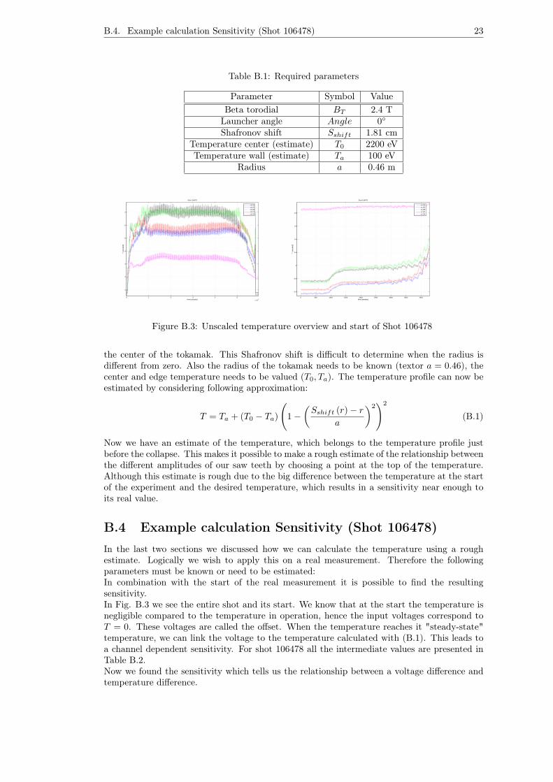
B.4 Example calculation Sensitivity (Shot 106478)In the last two sections we discussed how we can calculate the temperature using a roughestimate. Logically we wish to apply this on a real measurement. Therefore the followingparameters must be known or need to be estimated:In combination with the start of the real measurement it is possible to find the resultingsensitivity.In Fig. B.3 we see the entire shot and its start. We know that at the start the temperature isnegligible compared to the temperature in operation, hence the input voltages correspond toT = 0. These voltages are called the offset. When the temperature reaches it "steady-state"temperature, we can link the voltage to the temperature calculated with (B.1). This leads toa channel dependent sensitivity. For shot 106478 all the intermediate values are presented inTable B.2.Now we found the sensitivity which tells us the relationship between a voltage difference andtemperature difference.

24 Appendix B. Inversion radius

Table B.2: Intermediate values and resulting sensitivity

Channel [GHz] Testimate [eV] Offset (t = 0) [V] VECE (t = 3.3 s) [V] ∆V [V] Sens (Test/∆V ) [eV/V]132.5 2181 0.63 6.00 5.37 406.15135.5 2104 0.57 5.60 5.03 418.29138.5 1977 0.75 7.10 6.36 310.85141.5 1811 0.77 7.35 6.59 274.81144.5 1617 1.85 3.64 1.79 903.35

B.5 Amplitude versus wavelet coefficients

Next step to calculate the inversion radius is determining the sawtooth’s signal amplitude,which still is unknown. The best way is to determine the minimum and maximum of thesawtooth signal (in eV) and calculate the resulting amplitude. However, this is not an easyprocess to do real-time. Another possibility is to use frequency methods such as the ComplexMorlet Wavelet to determine an amplitude and phase but which is averaged. Both thesemethods expand the currently used algorithm for period detection considerably. Therefore it ischosen to use existing data-streams to make an estimate of the different amplitudes. From thereal-time wavelet analysis we already have calculated the wavelet coefficients, which alreadydescribe the direction of the crash. Their response is biggest in the highest scale m and weknow also that the magnitude of the wavelet coefficient is a measure for the dept of the crashi.e. the amplitude. Although it could be argued that they are not really linear dependent.Nevertheless we assume the magnitude of the wavelet coefficient is a good measure for theamplitude. It should be remembered that the wavelet coefficients only describe the amplitudenear a crash. We know that the highest scale wavelet coefficients are delayed more than thedetected value (threshold is lower). Therefore we just need to calculate the moment of a realcrash and add the delay and pick those values as our measure of amplitude. This is presentedin Fig. B.4.

1.5 2 2.5 3 3.5 4 4.5 5 5.5

x 105

−0.02

−0.015

−0.01

−0.005

0

0.005

0.01

0.015

0.02

Figure B.4: Wavelet coefficients different channels biggest scale m

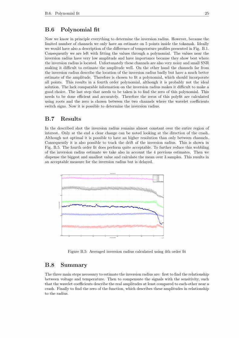
B.6. Polynomial fit 25

B.6 Polynomial fitNow we know in principle everything to determine the inversion radius. However, because thelimited number of channels we only have an estimate on 5 points inside the tokamak. Ideallywe would have also a description of the difference of temperature profiles presented in Fig. B.1.Consequently we are left with fitting the values through a polynomial. The values near theinversion radius have very low amplitude and have importance because they show best wherethe inversion radius is located. Unfortunately these channels are also very noisy and small SNRmaking it difficult to estimate the amplitude well. On the other hand the channels far fromthe inversion radius describe the location of the inversion radius badly but have a much betterestimate of the amplitude. Therefore is chosen to fit a polynomial, which should incorporateall points. This results in a fourth order polynomial, although it is probably not the idealsolution. The lack comparable information on the inversion radius makes it difficult to make agood choice. The last step that needs to be taken is to find the zero of this polynomial. Thisneeds to be done efficient and accurately. Therefore the zeros of this polyfit are calculatedusing roots and the zero is chosen between the two channels where the wavelet coefficientsswitch signs. Now it is possible to determine the inversion radius.

B.7 ResultsIn the described shot the inversion radius remains almost constant over the entire region ofinterest. Only at the end a clear change can be noted looking at the direction of the crash.Although not optimal it is possible to have an higher resolution than only between channels.Consequently it is also possible to track the drift of the inversion radius. This is shown inFig. B.5. The fourth order fit does perform quite acceptable. To further reduce this wobblingof the inversion radius estimate we take also in account the 4 previous estimates. Then wedispense the biggest and smallest value and calculate the mean over 3 samples. This results inan acceptable measure for the inversion radius but is delayed.

1.5 2 2.5 3 3.5 4 4.5 5

x 105

130

135

140

145

time [samples]

Fre

quen

cy [G

Hz]

Shot 106478

ec132ec135ec138ec141ec144inversion radius

Figure B.5: Averaged inversion radius calculated using 4th order fit

B.8 SummaryThe three main steps necessary to estimate the inversion radius are: first to find the relationshipbetween voltage and temperature. Then to compensate the signals with the sensitivity, suchthat the wavelet coefficients describe the real amplitudes at least compared to each-other near acrash. Finally to find the zero of the function, which describes these amplitudes in relationshipto the radius.

Appendix C

Tuning and practical considerations

In this appendix the different tuning parameters are discussed and some practical implemen-tation suggestions are made.

Block-timeThe block-time is the time that the wavelet coefficients are suppressed after detection has takenplace. This is done to prevent multiple detection on the same crash. This block-time is relatedto the size of the wavelet. Therefore it is chosen as the delay of the biggest wavelet addedby some extra time. This extra time should be chosen such that the wavelet coefficients arebelow the threshold again for the responses on the biggest wavelet. It also needs to be takeninto account that when wavelets are near the size of twice the period, the next crash could beblocked accidently when the same block-time applies to all scales (currently implemented assuch). This can be partially solved by making the block-time scale dependent. Then the smallscales can detect new crashes in an earlier stadium again.

Buffer sizeThe buffer stores the maxima of the responses. This in the form of logicals (0-1) such that itis implemented efficiently. The buffer-size can be chosen as big as one wants the minimum sizeshould be about the maximum delay of the biggest wavelet (preferably somewhat bigger).

PrefilterThe prefilter should be chosen such that crashes can generally be recognized but not suchthat they become very big. This is because the first scale is used to find the position of thecrash and should not be used for detection. In addition if the threshold is coupled to thefirst scale, high responses will lead to a too high threshold. Although tuning in the frequencydomain is a possibility, it is more difficult because the crash stands in relationship to thenoise. Consequently, the Fourier transform should be calculated carefully such that it does notaverages out the noise.

ThresholdIn the simulink algorithm two possible choices of the threshold are implemented. This isthe threshold purely based on the noise and the one based on the first scale of the waveletcoefficients (used in this thesis). The first, purely based on the noise works well in cleanregimes with not to much dynamical behavior. However, the underbound Tmin is somewhat tolow because not only noise is present. A factor 3-4 generally works well, however, in channelsnear the inversion radius, where the noise is much more significant a somewhat lower thresholdis necessary.The threshold based on the wavelet coefficients of the first scales is more robust for regimeswith significant dynamical behavior because the wavelet coefficients react on small crashes such

27

28 Appendix C. Tuning and practical considerations

that they are taken into account in the threshold. This also means that the threshold becomesdependent on the choice of the prefilter, which determines the size of the wavelet at the firstscale (factor 1.5-2.5) . Both the thresholds are currently based on a clock basis (few periods).This has the advantage compared to a crash based reset if crashes are missed, the threshold isautomatically re-adjusted. It is important to note that to prevent instant loss of the thresholdby activation and shutting down the NBI system due to the huge edges. Therefore during theseevents threshold updates need to be suppressed temporarily. The threshold can be improvedby implementing a continuous changing threshold (using FIR-filter).

Distance between maximaThe distance between maxima is used to prevent the maxima chain to wrong maxima. Itshould be chosen tight when dealing with strange crashes. In normal regimes it can be chosensomewhat less tight. Although generally the maxima are situated within a few samples fromeach other anyway. At the bigger scales, maxima are far apart, therefore the maximum distancebetween maxima should be somewhat bigger for big wavelets.

ChannelsThis part of the algorithm needs further improvement. However, as implemented now, thechoice of the number of channels in which a crash is detected depends on the threshold. Ifchosen for a robust threshold the channels in which detection takes place can be 2-3. However,if a less robust threshold (less-delay) is chosen this should be about 4. It is important to alsoconsider the reset time of falsely detected crashes.

Bibliography

[1] M. van Berkel, Wavelets for Feature Detection;Theoretical background, Eindhoven Univer-sity of Technology Std., 2010.

[2] J. Oosterbeek, “Towards a self-aiming microwave antenna to stabilise fusion plasmas,” Ph.D.dissertation, Technische Universiteit Eindhoven, 2009.

29