Wavelet Exploratory Analysis of the FTSE

ALL SHARE Index

Antonios Antoniou a Constantinos E. Vorlow a,∗

aDurham Business School, University of Durham, Mill Hill Lane, Durham,DH13LB, UK.

Abstract

Wavelets by construction are able to show us “the forest as well as the trees”.They are compactly supported functions that allow us to localise in frequency aswell as in time whereas traditional Fourier analysis focuses only on frequency. Thismakes wavelets useful when examining time sequences that exhibit sharp spikesand irregularities, such financial time series. In this paper we demonstrate how awavelet semi-parametric approach can provide useful insight on the structure andbehaviour of stock index prices, returns and volatility. By using wavelets we capturesalient features such as changes in trend and volatility and reveal dynamic patternsat various scales.

Key words: Wavelet transforms, scalograms, multiresolution analysis, financialtime series analysis.JEL classification: G14; C29; Z00.

∗ Corresponding authorEmail addresses: Antonios.Antoniou@durham.ac.uk (Antonios Antoniou),

K.E.Vorloou@durham.ac.uk (Constantinos E. Vorlow).URL: http://www.vorlow.org (Constantinos E. Vorlow).

Preprint submitted to WSEAS NOLASC 2003 20 November 2003

1 Introduction

Wavelets are becoming more popular as the academic community appreciatestheir ability to detect localised events as well as periodic structures. Originallyintroduced through financial and economic applications in the beginning of thelast decade, they have not yet enjoyed their deserved popularity. This is in co-ntrast to their potentially wide applicability and great versatility. Their abilityto isolate breaks and shifts in dynamics, to manipulate intermittent sequencesand their usefulness in denoising and smoothing makes them an important toolfor univariate time series analysis, comparable to that of ARIMA and spectralanalysis. The difference is that wavelets can provide the exact locality of anychanges in the dynamical patterns of the sequence whereas the other two tech-niques concentrate mainly on their frequency. 1 Moreover, Fourier transformsassume infinite-length signals, whereas wavelet transforms can be applied toany kind and size of time series, even when these sequences are not homogene-ously sampled in time. In general, wavelet transforms can be used to explore,denoise and smoothen financial time series, aid in forecasting, contribute toother empirical analysis frameworks (efficiency tests, event studies etc. etc.)and to calibrate or improve trading models. In this paper we aim to reintro-duce wavelet transforms with a more “digestible” demonstration. We showhow wavelet transforms can be applied and their results interpreted through avery simple exploratory framework. This approach can be of great interest topractitioners as it is avoids the pitfalls of a parametric model and statisticalhypothesis testing approach, while being fast and accurate. It also providesresults in various scales and frequencies, delivering a decomposition of greatdetail and information.

In the following sections we provide a brief outline of existing research in thearea of wavelet applications in finance and economics. Following this review,we present in section 2.1 a simple and brief introduction to the internals ofwavelet transforms and describe our database. We then explain in section 3how results of “time-scale” analysis can be interpreted and finally in section4 how wavelet transforms could be used in a discrete framework to providerudimentary data smoothing and noise filtering.

2 Past research

Strang (1989) and Graps (1995) provide an interesting introduction to the ge-neral subject (see also Ramsey, 2002). A more recent introduction, focused oneconomics, is Schleicher (2002). A very insightful and early paper is also Jensen

1 This excludes the case of Short Time Fourier Transforms.

2

(1997) who discusses the general potential of wavelets in financial empiricalresearch. One of the first applications were by Greenblatt (1996) who usedwavelets for outlier detection and Ramsey and Zaslavsky (1995) who influe-nce this paper. Jensen (1994) uses wavelets to estimate fractionally integratedprocesses. He shows an alternative way to estimate the fractional differencingparameter and shows the advantages of wavelets over the existing method ofGeweke and Porter-Hudak (1983). Continuing, Jensen (1999a) and (1999b)explores more deeply the applicability of wavelet transforms in long memorymodels. Olmeda and Fernandez (2000) provide a criticism of the theory bydrawing our attention to the pitfalls of using wavelet filtering for denoisingand forecasting purposes. Capobianco (2001), uses wavelets for describing fi-nancial returns processes. He studies the Nikkei stock index in high frequencyand shows results about modelling with GARCH when the data have beenpreprocessed by wavelets transforms. He demonstrates that one can obtainbetter volatility prediction power for one-step-ahead forecasts, implying thatlatent volatility features can be detected more efficiently. Capobianco (2002)uses multiresolution analysis to approximate volatility processes. He focuseson intra-day dynamics and again shows how wavelet transforms can improveour view of volatility dynamics provided by a GARCH specification on wave-let pre-processed sequences (see also Capobianco, 1999). Antoniou and Volrow(2003), in a similar approach to that of Chen (1996), use wavelets to denoiseindex returns from various countries and obtain evidence of deterministic non-linearities. Los and Karuppiah (2000) apply wavelet multiresolution analysison high-frequency Asian FX rates, in support to the Fractal Market Hypothe-sis of Mandelbrot (1966) and Peters (1994). Recently, Jamdee and Los (2003)examine the risk profile of the US term structure by the use of wavelet sca-lograms and multiresolution analysis, suggesting that the term structure ofinterest rate is segmented and that the basic assumptions of the “traditional”models are violated. In a recent extensive work, Los (2003) focuses in financialmarkets even more. In this extensive work wavelets and multiresolution analy-sis are used to measure persistence and to provide explanations on financialcrises, turbulence and volatility.

In this paper we use wavelets in a continuous and discrete multiresolution fra-mework to show their usefulness in the empirical investigation of asset pricedynamics. Our work follows the research of Ramsey and Zhifeng (1994), Ram-sey and Zhifeng (1995) and Ramsey and Lampart (1998). The necessary th-eoretical background for our approach is discussed in depth in Gencay et al.(2001) and Percival and Walden (2000). A very gentle introduction is Hub-bard (1998) and Ogden (1997) is more focused on the statistical aspect ofthe theory. A thorough treatment of wavelet theory is Strang and Nguyen(1996) and interesting on-line starting point and resource is the Wavelet Di-gest: http://www.wavelet.org.

3

2.1 Data description & methodology

The data set consists of 8192 daily observations of the FTSE ALL SHARE in-dex closing prices. Furthermore, we investigate the continuously compoundedreturns of the FTSE and the realised volatility of these returns. All daily se-quences start form the 10th of July 1970 and end the 30th of November 2001.In table 1 we display the descriptive statistics for the FTSE index, its logari-thmic returns and the realised volatility. From this table and the inspection ofthe relevant distribution histograms 2 we can deduce that the distribution ofthe closing prices of the FTSE index is positively skewed whereas the corre-sponding returns are leptokurtic and the realised volatility positively skewedas well. The Jarque-Bera test (see Bera and Jarque, 1981) for normality cle-arly rejects the null for all sequences, as expected. In general, the sequencesanalysed here follow closely the stylised facts as these are described in Cont(2001).

[insert table 1 about here]

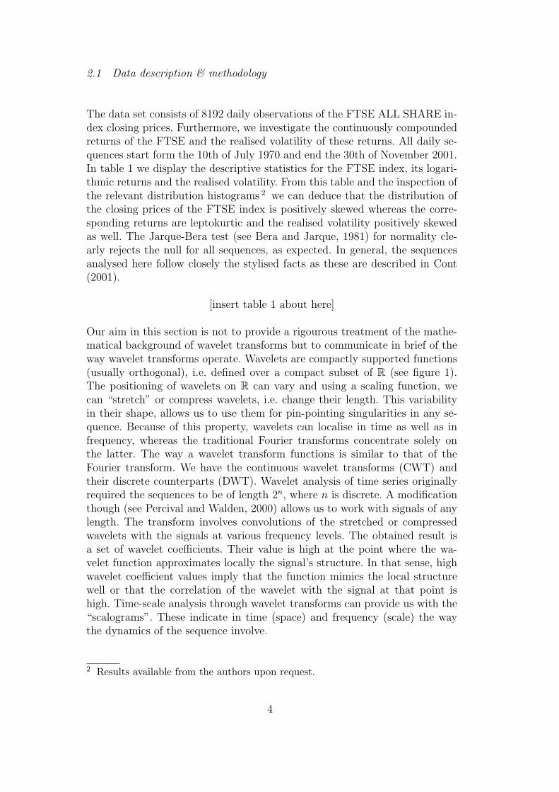
Our aim in this section is not to provide a rigourous treatment of the mathe-matical background of wavelet transforms but to communicate in brief of theway wavelet transforms operate. Wavelets are compactly supported functions(usually orthogonal), i.e. defined over a compact subset of R (see figure 1).The positioning of wavelets on R can vary and using a scaling function, wecan “stretch” or compress wavelets, i.e. change their length. This variabilityin their shape, allows us to use them for pin-pointing singularities in any se-quence. Because of this property, wavelets can localise in time as well as infrequency, whereas the traditional Fourier transforms concentrate solely onthe latter. The way a wavelet transform functions is similar to that of theFourier transform. We have the continuous wavelet transforms (CWT) andtheir discrete counterparts (DWT). Wavelet analysis of time series originallyrequired the sequences to be of length 2n, where n is discrete. A modificationthough (see Percival and Walden, 2000) allows us to work with signals of anylength. The transform involves convolutions of the stretched or compressedwavelets with the signals at various frequency levels. The obtained result isa set of wavelet coefficients. Their value is high at the point where the wa-velet function approximates locally the signal’s structure. In that sense, highwavelet coefficient values imply that the function mimics the local structurewell or that the correlation of the wavelet with the signal at that point ishigh. Time-scale analysis through wavelet transforms can provide us with the“scalograms”. These indicate in time (space) and frequency (scale) the waythe dynamics of the sequence involve.

2 Results available from the authors upon request.

4

Representing a time-series as a function f(t), the CWT of this function isdefined as:

Wψ(a, b) =1√a

∞∫

−∞f(t)ψ(

t− b

a)dt (1)

and the inverse transform is defined as:

f(t) =1

Cψ

∞∫

−∞

∞∫

−∞

1

a2[Wψ(a, b)]

1√aψ(

t− b

a)dadb, (2)

where ψ(t) is the “mother” wavelet and a, b ∈ R continuous variables witha 6= 0. The parameter a is called the “scale” or “dilation” parameter whichdetermines the level of stretch (expansion) or compression of the wavelet.Parameter “b” is called the “shift” or “translation” parameter. For low scalesi.e. when |a| ¿ 1, the wavelet function is highly concentrated (shrunken-compressed) with frequency contents mostly in the higher frequency bands.Inversely when |a| À 1, the wavelet is stretched and contains mostly lowfrequencies (for example: a time trend). For small scales we obtain thus a moredetailed view of the signal (known also as a “higher resolution”) whereas forlarger scales we obtain a more general view of the signal structure.

Continuous transforms provide us with a large amounts of redundant informa-tion. For this reason, there is a discrete version (DWT), generated by criticallysubsampling the coefficients of the CWT. This is conducted in such a way thatthe energy of the signal is preserved. DWT is faster and useful for denoisingand providing smoothed versions of the sequences at various discrete levelsof analysis. In the following sections we will demonstrate how one can obtaininteresting qualitative information on the structure of financial time series byusing both continuous and discrete wavelet transforms.

3 Scalograms and time-scale analysis

For the time-scale analysis that follows, we utilise two wavelet functions: theHaar and the symmlet 8 (or s8 for short). These two “mother” wavelet fu-nctions are depicted in the two top subfigures of figure 1, together with theircorresponding “father” or scaling functions. These wavelets were chosen aftercareful experimentation. There is no general rule on how to select mother wa-velets. Usually a mother wavelet should exhibit a similar structure to thatof the analysed signal. Often this choice is not such a crucial issue. Any re-latively small (short) wavelet should be a suitable starting point (the Haar

5

usually excluded). Given that a wavelet should resemble the time series, thediscontinuous and blocky Haar is not really appropriate for our data. It isthough a very simple and economical function, with fast transforms. Moreo-ver, as we shall demonstrate, the qualitative information we obtain from thetime-scale analysis is not that different from that of the s8 wavelet. The s8mother function seems a more appropriate candidate and produces slightlymore detailed scalograms as opposed to the “chunky” Haar ones.

[insert figure 1 about here]

In figures 2 (a-c) we have produced the Haar and s8 scalograms for the first8000 observations of the FTSE closing prices, the corresponding logarithmicreturns and realised volatility. Darker regions in these scalograms correspondto higher wavelet transform coefficients. From an initial inspection, we caneasily discern that the s8 wavelet provides a finer decomposition (“thinner”)than the Haar for the returns (figure 2 (b)) and the realised volatility seque-nce (figure 2 (c)) due the discontinuous nature of the latter wavelet depictedin figure (1). Because of the smoothness of the s8 mother wavelet, the scalo-grams for that transform exhibit smoother transitions between low, mediumand high-valued wavelet coefficients, and produce clearer bifurcations. An inte-resting point here from the comparison of the Haar and s8 scalograms is thatfor both the levels and the transformations of the FTSE series, the messagethey deliver is the same.

By careful examination of the index closing prices scalograms in figure 2 (a),we can see that both the Haar and s8 CWT coefficients change patterns afterthe 3000th (mainly 4000th i.e. roughly the 1st half of the history of the series)observation onwards and especially from the short “booming” period beforethe 1987 crash. Until that point, the prices of the wavelet transform coefficientsare lower, indicative of the relative smoothness or lack of excessive volatilityand of very weak positive trend. Both Haar and s8 scalograms are quite simi-lar. For the larger scales of between 150 and 250 days though, the Haar basedscalogram reports wider and fewer periods of smaller coefficients than thatof the s8 wavelet. We attribute this to the structure of the mother waveletfunction itself. Through both scalograms though, we are able to discern thatfor the lower scales there is a relative absence of trend (i.e. of a low frequencycomponent) whereas for larger scales and larger time “windows”, a very weaktrend is more obvious for the first half of the index series. One may recognisethose as the darker areas (“tree trunk” like formations) i.e. collections of highcoefficients on the top of both scalograms in figure 2. It is obvious form thetwo scalograms that the wavelet coefficients are able to capture the changeof the pattern after the 4000th observation. They also reveal the increase involatility and trend of the series. The difference between the Haar and the s8based scalogram is more evident on the right bottom half of the graphs wherefor the s8 wavelet, one can identify more easily the bifurcations formed by the

6

coefficients (see also details of scalograms in figure 3). This shows mainly howsmall and large sequences of coefficients interchange and may imply a mul-tifractal structure or some kind of non-periodic seasonality (see also Ramseyand Zaslavsky, 1995). See Wornel (1993 and 1995) for an extensive treatmentof the relevant theoretical background and framework regarding this issue.

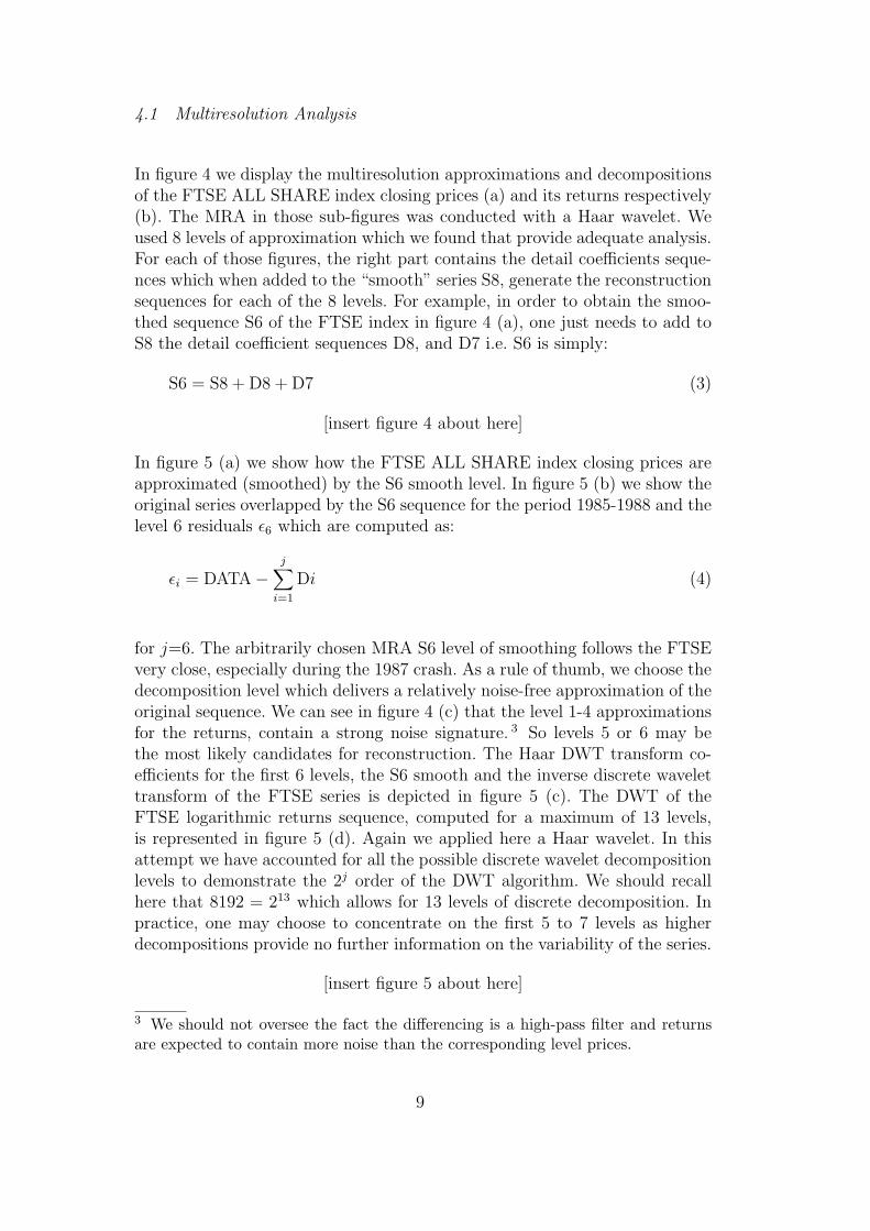
The patterns discussed so far, clearly change for the last half of the series. It isobvious from the time series plot of figure 2 (a), that there is a increase of thesteepness and the variance of the index sequence. This follows up historicallythe occurrence of the 1987 stock market crash. The crash occurs in the vicinityon the 4500th x-axis coordinate, where both Haar and s8 scalograms show aconcentration of high coefficients on all scales (shown as an inverted darkpeak). We see that regardless of the choice of the mother wavelet, the actualtiming of the crash of 1987 is detected successfully. Following that point, thevolatility of the series seems to increase considerably with finer bifurcationsof wavelet coefficients occurring in low, medium and large scales. It is obviousthat the frequency and the intensity of the aperiodic cycle structures haschanged for the last half of the series. The keen eye can also identify the restof the famous crises as they occur after observation 7000 such as the Asiancrisis, the NASDAQ and others. These and the effect of the incident of the11th of September 2001 can be seen in figure 3 (a) where we have producedthe s8 based scalogram of the whole 8192 FTSE ALL SHARE observations.In our analysis so far we choose to limit to the first 8000 observations inorder to exclude the intensive fluctuations of the last part of the history of theseries. Although our discrete and continuous analysis has included all 8192observations, we choose to truncate the sample in order to avoid depictingthe large valued coefficients at the end of the scalograms by excluding 192points. We do this as we are mainly interested in the 1987 crash which seemsmore isolated and clear to interpret (we can examine though the scalogramof this last cluster of observations at the end of figure 3 (a)). We can thusconcentrate on the oil crisis, the 1987 and Asian markets crashes and avoid the“blurring” of the results at the right edge of the series because of the increasedconcentration of high valued coefficients due to the clustering of well knownrecent events (mainly September the 11th). It would be interesting though tosee in a couple of years how these scalograms would have “evolved” with theinclusion of the recent and future history of the series.

In figure 3 (a), we can clearly detect after the vertical barrier line, the changein the scalogram’s pattern. We can also locate the intense oscillations followingthe Asian crisis, the NASDAQ crash and the September the 11th events atthe darker regions of the right edge of the scalogram. An interesting point isthat the oil crisis of the 70s is not that evident from the levels of the indexas in the scalograms of the returns and realised volatility. This is more clearlyshown in figure 2 (d), where we show the s8 scalograms from figures 2 (a-c),side by side for comparison purposes.

7

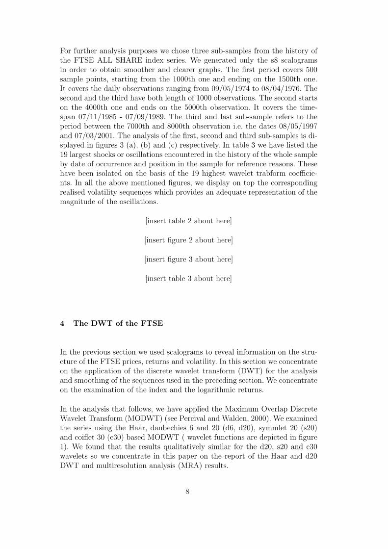
For further analysis purposes we chose three sub-samples from the history ofthe FTSE ALL SHARE index series. We generated only the s8 scalogramsin order to obtain smoother and clearer graphs. The first period covers 500sample points, starting from the 1000th one and ending on the 1500th one.It covers the daily observations ranging from 09/05/1974 to 08/04/1976. Thesecond and the third have both length of 1000 observations. The second startson the 4000th one and ends on the 5000th observation. It covers the time-span 07/11/1985 - 07/09/1989. The third and last sub-sample refers to theperiod between the 7000th and 8000th observation i.e. the dates 08/05/1997and 07/03/2001. The analysis of the first, second and third sub-samples is di-splayed in figures 3 (a), (b) and (c) respectively. In table 3 we have listed the19 largest shocks or oscillations encountered in the history of the whole sampleby date of occurrence and position in the sample for reference reasons. Thesehave been isolated on the basis of the 19 highest wavelet trabform coefficie-nts. In all the above mentioned figures, we display on top the correspondingrealised volatility sequences which provides an adequate representation of themagnitude of the oscillations.

[insert table 2 about here]

[insert figure 2 about here]

[insert figure 3 about here]

[insert table 3 about here]

4 The DWT of the FTSE

In the previous section we used scalograms to reveal information on the stru-cture of the FTSE prices, returns and volatility. In this section we concentrateon the application of the discrete wavelet transform (DWT) for the analysisand smoothing of the sequences used in the preceding section. We concentrateon the examination of the index and the logarithmic returns.

In the analysis that follows, we have applied the Maximum Overlap DiscreteWavelet Transform (MODWT) (see Percival and Walden, 2000). We examinedthe series using the Haar, daubechies 6 and 20 (d6, d20), symmlet 20 (s20)and coiflet 30 (c30) based MODWT ( wavelet functions are depicted in figure1). We found that the results qualitatively similar for the d20, s20 and c30wavelets so we concentrate in this paper on the report of the Haar and d20DWT and multiresolution analysis (MRA) results.

8

4.1 Multiresolution Analysis

In figure 4 we display the multiresolution approximations and decompositionsof the FTSE ALL SHARE index closing prices (a) and its returns respectively(b). The MRA in those sub-figures was conducted with a Haar wavelet. Weused 8 levels of approximation which we found that provide adequate analysis.For each of those figures, the right part contains the detail coefficients seque-nces which when added to the “smooth” series S8, generate the reconstructionsequences for each of the 8 levels. For example, in order to obtain the smoo-thed sequence S6 of the FTSE index in figure 4 (a), one just needs to add toS8 the detail coefficient sequences D8, and D7 i.e. S6 is simply:

S6 = S8 + D8 + D7 (3)

[insert figure 4 about here]

In figure 5 (a) we show how the FTSE ALL SHARE index closing prices areapproximated (smoothed) by the S6 smooth level. In figure 5 (b) we show theoriginal series overlapped by the S6 sequence for the period 1985-1988 and thelevel 6 residuals ε6 which are computed as:

εi = DATA−j∑

i=1

Di (4)

for j=6. The arbitrarily chosen MRA S6 level of smoothing follows the FTSEvery close, especially during the 1987 crash. As a rule of thumb, we choose thedecomposition level which delivers a relatively noise-free approximation of theoriginal sequence. We can see in figure 4 (c) that the level 1-4 approximationsfor the returns, contain a strong noise signature. 3 So levels 5 or 6 may bethe most likely candidates for reconstruction. The Haar DWT transform co-efficients for the first 6 levels, the S6 smooth and the inverse discrete wavelettransform of the FTSE series is depicted in figure 5 (c). The DWT of theFTSE logarithmic returns sequence, computed for a maximum of 13 levels,is represented in figure 5 (d). Again we applied here a Haar wavelet. In thisattempt we have accounted for all the possible discrete wavelet decompositionlevels to demonstrate the 2j order of the DWT algorithm. We should recallhere that 8192 = 213 which allows for 13 levels of discrete decomposition. Inpractice, one may choose to concentrate on the first 5 to 7 levels as higherdecompositions provide no further information on the variability of the series.

[insert figure 5 about here]

3 We should not oversee the fact the differencing is a high-pass filter and returnsare expected to contain more noise than the corresponding level prices.

9

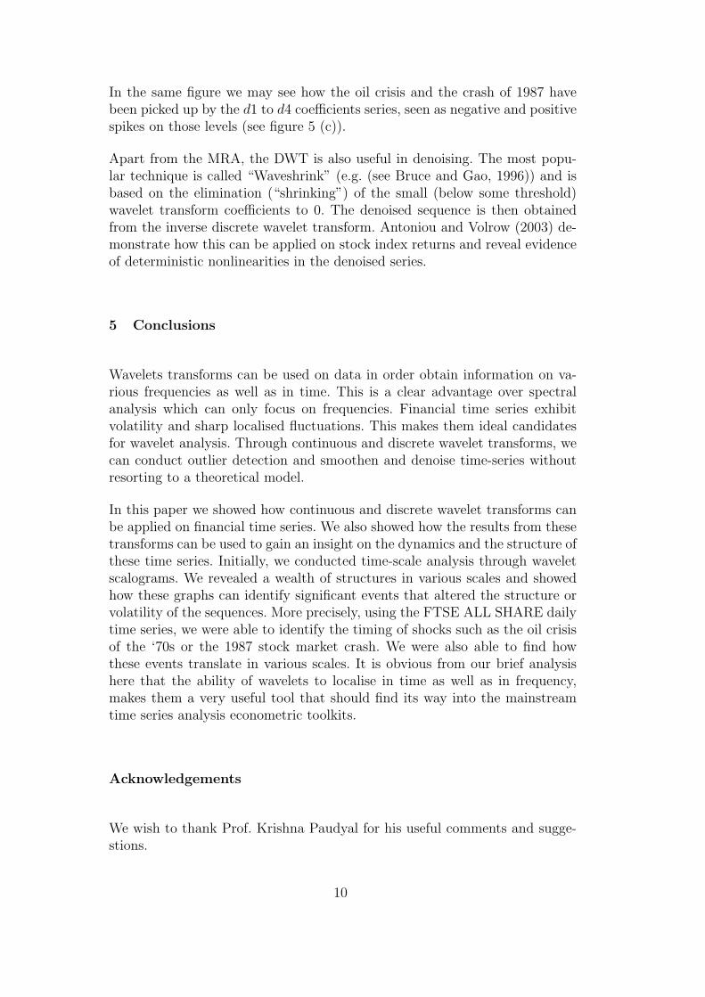
In the same figure we may see how the oil crisis and the crash of 1987 havebeen picked up by the d1 to d4 coefficients series, seen as negative and positivespikes on those levels (see figure 5 (c)).

Apart from the MRA, the DWT is also useful in denoising. The most popu-lar technique is called “Waveshrink” (e.g. (see Bruce and Gao, 1996)) and isbased on the elimination (“shrinking”) of the small (below some threshold)wavelet transform coefficients to 0. The denoised sequence is then obtainedfrom the inverse discrete wavelet transform. Antoniou and Volrow (2003) de-monstrate how this can be applied on stock index returns and reveal evidenceof deterministic nonlinearities in the denoised series.

5 Conclusions

Wavelets transforms can be used on data in order obtain information on va-rious frequencies as well as in time. This is a clear advantage over spectralanalysis which can only focus on frequencies. Financial time series exhibitvolatility and sharp localised fluctuations. This makes them ideal candidatesfor wavelet analysis. Through continuous and discrete wavelet transforms, wecan conduct outlier detection and smoothen and denoise time-series withoutresorting to a theoretical model.

In this paper we showed how continuous and discrete wavelet transforms canbe applied on financial time series. We also showed how the results from thesetransforms can be used to gain an insight on the dynamics and the structure ofthese time series. Initially, we conducted time-scale analysis through waveletscalograms. We revealed a wealth of structures in various scales and showedhow these graphs can identify significant events that altered the structure orvolatility of the sequences. More precisely, using the FTSE ALL SHARE dailytime series, we were able to identify the timing of shocks such as the oil crisisof the ‘70s or the 1987 stock market crash. We were also able to find howthese events translate in various scales. It is obvious from our brief analysishere that the ability of wavelets to localise in time as well as in frequency,makes them a very useful tool that should find its way into the mainstreamtime series analysis econometric toolkits.

Acknowledgements

We wish to thank Prof. Krishna Paudyal for his useful comments and sugge-stions.

10

References

Antoniou, A., Volrow, C. E., 2003. Recurrence quantification analysis of wave-let pre-filtered index returns. Tech. rep., University of Durham, Economics& Finance, Discussion Paper Series.

Bera, A., Jarque, C., 1981. Efficient Tests for Normality, Heteroskedasticityand Serial Independence of Regression Residuals: Monte-Carlo evidence.Economics Letters 7, 313–318.

Bruce, A., Gao, H.-Y., 1996. Understanding WaveShrink: Variance and biasestimation. Biometrika 83 (4).URL ftp://ftp.statsci.com/pub/gao/varbias.ps.Z

Capobianco, E., 1999. Statistical Analysis of Financial Volatility by WaveletShrinkage. Methodology And Computing In Applied Probability 1 (4), 423–443.

Capobianco, E., 2001. Wavelet Transforms for the Statistical Analysis of Re-turns Generating Stochastic Processes. International Journal of Theoreticaland Applied Finance 4 (3), 511–34.

Capobianco, E., 2002. Multiresolution Approximation for Volatility Process.Quantitative Finance 2 (2), 91–110.

Chen, P., 1996. A random walk or color chaos on the stock market? time-frequency analysis of S&P indexes. Studies in Nonlinear Dynamics andEconometrics 1 (2), 87–103.

Cont, R., 2001. Empirical properties of asset returns: Stylized facts and stati-stical issues. Quantitative Finance 1 (2), 223–36.

Gencay, R., Selcuk, F., Whitcher, B., 2001. An Introduction to Wavelets andOther Filtering Methods in Finance and Economics. Academic Press, SanDiego.

Geweke, J., Porter-Hudak, S., 1983. The estimation and application of longmemory time series models. Journal of Time Series Analysis 4, 221–238.

Graps, A. L., 1995. An Introduction to Wavelets. IEEE Computational Scie-nces and Engineering 2 (2), 50–61.

Greenblatt, S. A., 1996. Wavelets in econometrics: An application to outliertesting. In: Gilli, M. (Ed.), Computational Economic Systems: Models, Me-thods & Econometrics. Vol. 5 of Advances in Computational Economics.Kluwer Academic Publishers, Dordrecht, pp. 139–160.

Hubbard, B. B. A., 1998. The World According to Wavelets: The Story of aMathematical Technique in the Making, 2nd Edition. A K Peters LimitedPublisher Record, Natick.

Jamdee, S., Los, C. A., January 2003. Dynamic Risk Profile of the US TermStructure by Wavelet MRA. Working paper, Kent State University, Depart-ment of Finance.

Jensen, M. J., 1994. Wavelet Analysis of Fractionally Integrated Processes.Working paper, University of Missouri.

Jensen, M. J., 1997. Making wavelets in finance. Financial Engineering News(1), 1–10.

11

Jensen, M. J., 1999a. An Approximate Wavelet MLE of Short- and Long-Memory Parameters. Studies in Nonlinear Dynamics and Econometrics3 (4), 239–53.

Jensen, M. J., 1999b. Using wavelets to obtain a consistent ordinary leastsquares estimator of the fractional differencing parameter. Journal of Fore-casting 18, 17–32.

Los, C. A., July 2003. Financial Market Risk: Measurement & Analysis. Rout-ledge International Studies in Money and Banking. Taylor & Francis BooksLtd, London, UK.

Los, C. A., Karuppiah, J., December 2000. Wavelet Multiresolution Analysisof High-Frequency Asian FX Rates. In: Quantitative Methods in Finance& Bernoulli Society 2000 Conference. University of Technology, Sydney,Australia, pp. 171–198.

Mandelbrot, B. B., 1966. Forecasts of Future Prices, Unbiased Markets andMartingale Models. Journal of Business 39 ((Special Supplement)), 242–255.

Ogden, R. T., 1997. Essential wavelets for statistical applications and dataanalysis. Birkhuser.

Olmeda, I., Fernandez, E., 2000. Filtering with wavelets may be worst than youthink. In: Computing in Economics and Finance, Society for ComputationalEconomics.

Percival, D. B., Walden, A. T., 2000. Wavelet Methods for Time Series Analy-sis. Cambridge University Press, New York, series in Statistical and Proba-bilistic Mathematics, No. 4.

Peters, E. E., 1994. Fractal market analysis : applying chaos theory to invest-ment and economics. J. Wiley & Sons, New York.

Ramsey, J. B., October 2002. Wavelets in economics and finance: Past andfuture. Studies in Nonlinear Dynamics and Econometrics 6 (3), Article 1.

Ramsey, J. B., Lampart, C., 1998. The decomposition of economic relation-ships by time scale using wavelets: Expenditure and income. Studies inNonlinear Dynamics and Econometrics 3 (1), 23–42.

Ramsey, J. B., Zaslavsky, G. M., 1995. An Analysis of U.S. Stock Price Beh-aviour Using Wavelets. Fractals 3, 377–389.

Ramsey, J. B., Zhifeng, Z., 1994. The application of wave form dictionaries tostock market index data. Tech. Rep. 94-05, STAR Discussion Paper.

Ramsey, J. B., Zhifeng, Z., 1995. The analysis of foreign exchange data usingwaveform dictionaries. Tech. Rep. 95-03, STAR Discussion Paper.

Schleicher, C., 2002. An Introduction to Wavelets for Economists. Tech. rep.,Bank of Canada Working Paper.

Strang, G., 1989. Wavelets and dilation equations: a brief introduction. SIAMReview 31, 614–627.

Strang, G., Nguyen, T. A., 1996. Wavelets and Filter Banks. Wellesley-Cambridge Press, Wellesley.

Wornell, G., 1993. Wavelet-based representation for the 1/f family of fractalprocesses. Proc. IEEE (Sept. 1993).

Wornell, G., 1995. Signal Processing with Fractals: A Wavelet Based approach.

12

Prentice Hall.

13

Table 1Descriptive statistics. Jarque-Bera p-values within parenthesis.

Statistic index returns realised volatility

minimum 61.92 -0.1191000 0.000e+000

Q1 221.60 -0.0048350 5.287e-006

median 768.90 0.0003343 2.859e-005

mean 1001.00 0.0003669 9.995e-005

Q3 1514.00 0.0058370 9.368e-005

maximum 3266.00 0.0894300 1.419e-002

st.deviation 899.0817 0.009992 0.000335

skewness 0.941687 -0.332639 19.48220

kurtosis 2.741635 12.32305 608.4498

Jarque-Berra 1233.378 (0.0) 29815.85 (0.0) 1.26e+08 (0.0)

Table 2The 3 subsamples used in figures 3, subfigures (b)-(c)

Subsample Dates Range Size

1 09/05/1974-08/04/1976 1000-1500 500

2 07/11/1985-07/09/1989 4000-5000 1500

3 08/05/1997-07/03/2001 7000-8000 1500

Table 3Dates and positions of th 19th largest oscillations in the FTSE series as these areidentified by the 19 largest DWT wavelet coefficients.

Dates Observation

06/12/1973 890

14/12/1973 896

01/03/1974 951

02/01/1975 1170

24/01/1975 1186

27/01/1975 1187

29/01/1975 1189

30/01/1975 1190

07/02/1975 1196

10/02/1975 1197

11/03/1975 1218

17/04/1975 1245

19/10/1987 4507

20/10/1987 4508

21/10/1987 4509

22/10/1987 4510

26/10/1987 4512

10/04/1992 5676

11/09/2001 8134

Mot

her

Wav

elet

Haar

0.0

0.2

0.4

0.6

0.8

1.0

-1.00.00.51.0

Sca

ling

Fun

ctio

n

0.0

0.2

0.4

0.6

0.8

1.0

0.00.40.8

Mot

her

Wav

elet

Symmlet 8

-20

24

-1.00.01.0

Sca

ling

Fun

ctio

n

02

46

-0.20.20.61.0

Mot

her

Wav

elet

Symmlet 20

-50

510

-0.50.51.0

Sca

ling

Fun

ctio

n

05

1015

-0.20.20.61.0

Mot

her

Wav

elet

Daubechies 20

-50

510

-1.0-0.50.00.5

Sca

ling

Fun

ctio

n

05

1015

-0.40.00.40.8

Mot

her

Wav

elet

Coiflet 30

-15

-10

-50

510

15

-0.50.00.51.0

Sca

ling

Fun

ctio

n

-10

-50

510

1520

-0.20.20.61.0

Fig

.1.

Wav

elet

san

dsc

alin

gfu

ncti

ons:

Haa

r,Sy

mm

let

8an

d20

,D

aube

chie

s20

,C

oifle

t30

050

010

0015

0020

0025

0030

0035

0040

0045

0050

0055

0060

0065

0070

0075

0080

000

500

1000

1500

2000

2500

3000

3500

FT

SE

ALL

SH

AR

E in

dex

clos

ing

pric

es

Haa

r C

WT

Scale

050

010

0015

0020

0025

0030

0035

0040

0045

0050

0055

0060

0065

0070

0075

0080

00 1 14

27

40

53

66

79

92

105

118

131

144

157

170

183

196

209

222

235

248

Sym

mle

t 8 C

WT

Tim

e

Scale

050

010

0015

0020

0025

0030

0035

0040

0045

0050

0055

0060

0065

0070

0075

0080

00 1 14

27

40

53

66

79

92

105

118

131

144

157

170

183

196

209

222

235

248

(a)

Clo

sing

pric

es

050

010

0015

0020

0025

0030

0035

0040

0045

0050

0055

0060

0065

0070

0075

0080

00−

0.2

−0.

10

0.1

0.2

FT

SE

loga

rithm

ic r

etur

ns

Haa

r C

WT

Scale

050

010

0015

0020

0025

0030

0035

0040

0045

0050

0055

0060

0065

0070

0075

0080

00 1 14

27

40

53

66

79

92

105

118

131

144

157

170

183

196

209

222

235

248

Sym

mle

t 8 C

WT

Tim

e

Scale

050

010

0015

0020

0025

0030

0035

0040

0045

0050

0055

0060

0065

0070

0075

0080

00 1 14

27

40

53

66

79

92

105

118

131

144

157

170

183

196

209

222

235

248

(b)

Ret

urns

050

010

0015

0020

0025

0030

0035

0040

0045

0050

0055

0060

0065

0070

0075

0080

00

051015x

10−

3F

TS

E r

ealis

ed v

olat

ility

Haa

r C

WT

Scale

050

010

0015

0020

0025

0030

0035

0040

0045

0050

0055

0060

0065

0070

0075

0080

00 1 1

4 2

7 4

0 5

3 6

6 7

9 9

210

511

813

114

415

717

018

319

620

922

223

524

8

Sym

mle

t 8 C

WT

Tim

e

Scale

050

010

0015

0020

0025

0030

0035

0040

0045

0050

0055

0060

0065

0070

0075

0080

00 1 1

4 2

7 4

0 5

3 6

6 7

9 9

210

511

813

114

415

717

018

319

620

922

223

524

8

(c)

Rea

lised

Vol

atili

ty

FT

SE

CW

T u

sing

sym

mle

t 8 w

avel

et

scales

050

010

0015

0020

0025

0030

0035

0040

0045

0050

0055

0060

0065

0070

0075

0080

00 1 14

27

40

53

66

79

92

105

118

131

144

157

170

183

196

209

222

235

248

FT

SE

ret

urns

CW

T u

sing

sym

mle

t 8 w

avel

et

scales0

500

1000

1500

2000

2500

3000

3500

4000

4500

5000

5500

6000

6500

7000

7500

8000

1 14

27

40

53

66

79

92

105

118

131

144

157

170

183

196

209

222

235

248

FT

SE

rea

lised

vol

atili

ty u

sing

sym

mle

t 8 w

avel

et

time

scales

050

010

0015

0020

0025

0030

0035

0040

0045

0050

0055

0060

0065

0070

0075

0080

00 1 14

27

40

53

66

79

92

105

118

131

144

157

170

183

196

209

222

235

248

(d)

Com

pari

son

ofs8

Fig

.2.

Tim

e-sc

ale

anal

ysis

ofth

eFT

SEcl

osin

gpr

ices

,re

turn

san

dvo

lati

lity.

1000

2000

3000

4000

5000

6000

7000

8000

500

1000

1500

2000

2500

3000

Ana

lyze

d S

igna

l

Sca

le o

f col

ors

from

MIN

to M

AX

Val

ues

of C

a,b

Coe

ffici

ents

for

a =

[1:1

:250

] −−

Col

orat

ion

mod

e : i

nit +

by

scal

e +

abs

1000

2000

3000

4000

5000

6000

7000

8000

1

14

27

40

53

66

79

92

105

118

131

144

157

170

183

196

209

222

235

248

(a)

10/0

7/19

70ti

ll30

/11/

2001

010

020

030

040

050

0−

1.2

0.8

2.8

4.8

6.8

8.8

x 10

−3

FT

SE

rea

lised

vol

atili

ty

F

TS

E A

LL S

HA

RE

inde

x cl

osin

g pr

ices

CW

T

Scale

010

020

030

040

050

0 1 1

4 2

7 4

0 5

3 6

6 7

9 9

210

511

813

114

415

717

018

319

620

922

223

524

8

FT

SE

loga

rithm

ic r

etur

ns C

WT

Scale

010

020

030

040

050

0 1 1

4 2

7 4

0 5

3 6

6 7

9 9

210

511

813

114

415

717

018

319

620

922

223

524

8

FT

SE

rea

lised

vol

atili

ty C

WT

TIM

E

Scale

010

020

030

040

050

0 1 1

4 2

7 4

0 5

3 6

6 7

9 9

210

511

813

114

415

717

018

319

620

922

223

524

8

(b)

09/0

5/19

74ti

ll08

/04/

1976

010

020

030

040

050

060

070

080

090

010

00

051015x

10−

3F

TS

E r

ealis

ed v

olat

ility

F

TS

E A

LL S

HA

RE

inde

x cl

osin

g pr

ices

CW

T

Scale

010

020

030

040

050

060

070

080

090

010

00 1 1

4 2

7 4

0 5

3 6

6 7

9 9

210

511

813

114

415

717

018

319

620

922

223

524

8

FT

SE

loga

rithm

ic r

etur

ns C

WT

Scale

010

020

030

040

050

060

070

080

090

010

00 1 1

4 2

7 4

0 5

3 6

6 7

9 9

210

511

813

114

415

717

018

319

620

922

223

524

8

FT

SE

rea

lised

vol

atili

ty C

WT

TIM

E

Scale

010

020

030

040

050

060

070

080

090

010

00 1 1

4 2

7 4

0 5

3 6

6 7

9 9

210

511

813

114

415

717

018

319

620

922

223

524

8

(c)

07/1

1/19

85ti

ll07

/09/

1989

010

020

030

040

050

060

070

080

090

010

00

051015x

10−

4F

TS

E r

ealis

ed v

olat

ility

F

TS

E A

LL S

HA

RE

inde

x cl

osin

g pr

ices

CW

T

Scale

010

020

030

040

050

060

070

080

090

010

00 1 1

4 2

7 4

0 5

3 6

6 7

9 9

210

511

813

114

415

717

018

319

620

922

223

524

8

FT

SE

loga

rithm

ic r

etur

ns C

WT

Scale

010

020

030

040

050

060

070

080

090

010

00 1 1

4 2

7 4

0 5

3 6

6 7

9 9

210

511

813

114

415

717

018

319

620

922

223

524

8

FT

SE

rea

lised

vol

atili

ty C

WT

TIM

E0

100

200

300

400

500

600

700

800

900

1000

1 14

27

40

53

66

79

92

105

118

131

144

157

170

183

196

209

222

235

248

Scale

(d)

08/0

5/19

97ti

ll07

/03/

2001

Fig

.3.

Exa

min

ing

the

deta

ilsof

the

s8sc

alog

ram

sin

figur

e2.

0 2000 4000 6000 8000

S8

S7

S6

S5

S4

S3

S2

S1

Data

Multiresolution approximation

0 2000 4000 6000 8000

S8

D8

D7

D6

D5

D4

D3

D2

D1

Data

Multiresolution decomposition

(a) FTSE closing prices

0 2000 4000 6000 8000

S8

S7

S6

S5

S4

S3

S2

S1

Data

Multiresolution approximation

0 2000 4000 6000 8000

S8

D8

D7

D6

D5

D4

D3

D2

D1

Data

Multiresolution decomposition

(b) FTSE returns

Fig. 4. Multiresolution approximations and decompositions

07/1

0/19

7007

/10/

1976

07/1

0/19

8207

/10/

1988

07/1

0/19

9407

/10/

2000

Tim

e

0100020003000

FT

SE

inde

x cl

osin

g pr

ices

07/1

0/19

7007

/10/

1976

07/1

0/19

8207

/10/

1988

07/1

0/19

9407

/10/

2000

Tim

e

050010001500200025003000

S6

appr

oxim

atio

n w

ith a

Haa

r w

avel

et

(a)

FT

SEan

dS6

smoo

th

1985

1986

1986

1987

1987

1988

1988

Tim

e

7009001100

FT

SE

and

S6

betw

een

1985

and

198

8

11/0

7/19

8505

/07/

1986

11/0

7/19

8605

/07/

1987

11/0

7/19

8705

/07/

1988

11/0

7/19

88

Tim

e

-150-100-50050100150

Diff

eren

ce v

betw

een

FT

SE

and

S6

appr

oxim

atio

n

(b)

Ade

tail

from

subfi

gure

(a)

020

0040

0060

0080

00

s6d6d5d4d3d2d1

idw

t

(c)

Mul

tire

solu

tion

anal

ysis

07/1

0/19

7007

/10/

1976

07/1

0/19

8207

/10/

1988

07/1

0/19

9407

/10/

2000

Tim

e

-0.10-0.050.000.05

FT

SE

loga

rithm

ic r

etur

ns

020

0040

0060

0080

00

s13

d13

d12

d11

d10d9d8d7d6d5d4d3d2d1

idw

t

Haa

r D

W d

ecom

posi

tion

on 1

3 le

vels

(d)

The

DW

Tof

the

FT

Ere

turn

s

Fig

.5.