Wavelet Transform and Terahertz Local Tomography

Xiaoxia Yina and Brian W.-H. Nga and Bradley Fergusonab and Derek Abbotta

aCentre for Biomedical Engineering and School of Electrical & Electronic Engineering, TheUniversity of Adelaide, SA 5005, Australia;

bTenix - Electronic Systems Division 2nd Avenue, Technology Park, Mawson Lakes, SA 5095,Australia

ABSTRACT

We use the theory of two dimensional discrete wavelet transforms to derive inversion formulas for the Radontransform of terahertz datasets. These inversion formulas with good localised properties are implemented for thereconstruction of terahertz imaging in the area of interest, with a significant reduction in the required measure-ments. As a form of optical coherent tomography, terahertz CT complements the current imaging techniques andoffers a promising approach for achieving non-invasive inspection of solid materials, with potentially numerousapplications in industrial manufacturing and biomedical engineering.

Keywords: Terahertz, T-rays, wavelet, computed tomography (CT), filtered back projection (FBP)

1. INTRODUCTION

Terahertz radiation (T-rays) is a collective term to describe the part of the electromagnetic spectrum from 0.1THz to 10 THz.1–6 The application of THz time domain spectroscopy (THz-TDS), especially in the biomedicaland security fields and in the fields of material science, is attractive owing to two intrinsic properties: a non-ionising nature and the ability to penetrate dry, non-polar and non-metallic materials.7 Compared to traditionalX-ray techniques, terahertz 3D imaging uses coherent tomography, which allows us to obtain both phase andamplitude information of an object.

This paper for CT reconstruction is motivated by terahertz TDS imaging mechanisms and focuses on terahertzCT imaging with reduced projection angles. The main goal of this paper is to present a wavelet based recon-struction algorithm for terahertz computed tomography and to show how this algorithm can be used to rapidlyreconstruct the region of interest (ROI) with a reduction in the measurements of terahertz responses, comparedwith a standard reconstruction. The current algorithm provides new insight into the relationship between localreconstruction, local projection, and the resolution of terahertz coherent tomography. This algorithm is sensitiveto terahertz data when reconstructing local projections using wavelet techniques, resulting in variations in theboundary of the local projection region after the wavelet transform, which gives rise to different resolution andreconstructed image sizes. This algorithm generates the approximation and detail images separately, and thefinal reconstruction is found by inverse wavelet transform. The algorithm reconstructs the area of interest viaapplying two sets of data from two different target experiments: polystyrene with hold inside and a tube insidea vial—a simple nested structure. For the first datasets, we reconstruct (i) a center region of 16 pixel radiusin a 100 × 100 pixel image using 46% of full data; (ii) an off-centre region of radius 30 pixels in a 100 × 100image using 66% of full data. For the second set of datasets, we reconstruct a center region of 6 pixel radius ina 100 × 100 pixel radius image using 59% of full data.

This paper consists of six sections. Section II introduces a terahertz functional imaging system and gives anoverview of the nonlocality of the Radon transform — this is important because we review the difference betweenthe conventional Radon transform reconstruction and our modified Radon transform for coherent tomography.In addition, following review of traditional Radon transform, this section summarize the basics of the wavelettransform, and a full-data reconstruction technique based on the wavelet transform is also involved. Section IVthen discusses the implementation of this method, and in Section V, the tomographic results are presented.

Further author information: (Send correspondence to Derek Abbott)Derek Abbott: E-mail: dabbott@eleceng.adelaide.edu.au, Telephone: +61-8-8303-5748

Novel Optical Instrumentation for Biomedical Applications III, edited by Christian D. DepeursingeProc. of SPIE-OSA Biomedical Optics, SPIE Vol. 6631, 663113, © 2007 SPIE-OSA · 1605-7422/07/$18

SPIE-OSA Vol. 6631 663113-1

2. METHODOLOGY

2.1. A Brief Introduction to Terahertz Imaging

A terahertz CT system is based on a chirped terahertz time domain spectroscopy scanned imaging system.The target is mounted on a motion stage that allows it to be translated along the x and z axes. Meanwhile,the object can also be rotated and linearly moved. The detailed information for the chirped pulse scanning andrelative rectangular coordinate system and polar coordinates for imaging reconstruction please see.8 The currentresearch builds upon our previous work represented in Ferguson et al.8

2.2. An Overview of CT and Terahertz CT

Normally, a filtered back projection algorithm begins with a collection of sinograms obtained from projectionmeasurements. A sinogram is simply generated via a collection of the projections at all the projection angles. Itsatisfies the following equation:

s(ξ, θ) =∫o(x, z)dξ (1)

where all points on projection offset ξ satisfy the equation: x cos θ + z sin θ = ξ and o denotes the measuredimage intensity of a target object, which is a function of pixel position in an x and z plane.

The filtered back projection algorithm for terahertz CT reconstruction is expressed as follows:

I(x, y) =∫ π

0

[∫ ∞

−∞S(θ, β)|β|exp[i2πβξ]dβ

]dθ (2)

where S(θ, β) is the spatial Fourier transform of the parallel projection data, defined as

S(θ, β) =∫ ∞

−∞s(θ, ξ)exp[−i2πβξ]dξ, (3)

here, s(θ, ξ) is the measured projection data, β is the spatial frequency in the ξ direction. It should be notedthat the operation of the ramp filter |β|, as illustrated in Eq. (3), is equivalent to a differentiation followed by aHilbert transform, which introduces a discontinuity in the derivative of the Fourier transform at zero frequency,while wavelet based local reconstruction, represented in this paper, ensures localised features of a local basis forimage recovery.

2.2.1. Calculation of Terahertz Parameters for Reconstruction of Terahertz CT

One of the advantages that terahertz CT has over X-ray CT is that s(θ, ξ) may be one of several parametersderived from terahertz pulses. Fundamentally, a terahertz CT setup is capable of measuring the transmittedterahertz pulse as a function of time t, for a given projection angle and projection offset. In principle, terahertzsinograms can be obtained in both time and frequency domains:

Frequency domain sinogram for terahertz CT:

The measured terahertz pulse is a function of time t, at a given projection angle and projection offset pd(t, θ, ξ).Let us denote the Fourier transform of this time domain pulse by Pd(ω, θ, ξ). The reference pulse pi(t) and thecorresponding Fourier response Pi(ω) can be measured by removing the target object from background. If thetarget is rotated and probed by terahertz beams, Pd(ω, θ, ξ) may be evaluated by adding sufficient projectionangles to allow the filtered back projection algorithm to be applied at each specific frequency ω. This is basedon the approximation that the detected terahertz signal is viewed as a linear integral of the incident terahertzpulse,

Pd(ω, θ, ξ) = Pi(ω) exp

[∫L(θ,ξ)

−iωn(r)c

dr

](4)

where Pd and Pi are the Fourier transforms of the detected and incident terahertz signals, respectively; c isthe speed of light in free space, L is the projection path, a straight line between the source and detector. Theunknown complex refractive index of the sample is denoted by n(ω, r) = nδ(ω, r) + ik(ω, r), where nδ(ω, r) is

SPIE-OSA Vol. 6631 663113-2

the real refractive index deviation and k(ω, r) is the extinction coefficient, related to absorption coefficient α viak(ω, r) = α/2ki (ki is the incident extinction coefficient). Let us define that,

Pn.=

[Pd(θ, ξ)Pi(θ, ξ)

]/ki =

∫L

nδ(r)dr = �{nδ(r)} (5)

Pα.= −2

∥∥∥∥Pd(θ, ξ)Pi(θ, ξ)

∥∥∥∥ =∫

L

α(r)dr = �{α(r)} (6)

where arg(x) denotes the phase or argument of complex valued x, ‖ x ‖ denotes the magnitude of the complexscalar x, and Pn and Pα are the projection data inputs to the filtered back projection algorithm as required toreconstruct nδ and α, respectively, at a specific terahertz frequency ω. The sign r denotes the position of theincident field (the sensor). The frequency signogram is applied to the vial and tube data sets (see later) for thispaper’s experiments.Time domain signogram for terahertz CT: One of the advantages that terahertz CT has over X-ray CTis that s(θ, ξ) may be one of several parameters derived from terahertz pulses. Fundamentally, a terahertz CTsetup is capable of measuring the transmitted terahertz pulse as a function of time t, for a given projection angleand projection offset. In principle, terahertz sinograms can be obtained in both time and frequency domains. Inthis paper, we review the calculation of terahertz sinograms in the time domain.

This method is based on the assumption that the target is of less dispersion and therefore the THz pulseshape is less unchanged after propagation through the target apart from attenuation and time delay. A referenceterahertz pulse pi(t) is measured without the target in place. To estimate the phase shift t of a terahertz pulsepd(t), the two signals are resampled at a higher rate using low-pass interpolation. The two interpolated signalsare then cross-correlated, and the maximised cross-correlation product at each angle as the lag is taken as theestimation of the phase delay of pd(t).

Timing sinogram can be calculated based on the following equation

ptime =∫

L(θ,ξ)

Tdelaydr (7)

here, ptime denotes the sinogram image in the time domain, recovered from the maximum time delay. As fordetailed information for the time domain signogram calculation, please refer to Ferguson et al.8

2.3. Two Dimensional Wavelet Based CT Reconstruction2.3.1. Two Dimensional Wavelet Transform (2D DWT)

Wavelet transforms play an important role in many image processing algorithms. Fundamentally, wavelet de-composition corresponds to a multiresolution analysis of a signal.9–13 This has the advantage of much improvedjoint time-frequency localisation over Fourier based techniques. In practice, it is nearly always implemented usingdigital filters and downsamplers. In two dimensions, the discrete version of a wavelet transform can be realisedby a 2D scaling function, φ(x, y), and three 2D wavelets, ψ1(x, y), ψ2(x, y), and ψ3(x, y), which are calculated bytaking the 1D wavelet transform along the rows of f(x, y) and the resulting columns. The 2D scaling functionand 2D wavelet functions satisfy the equations represented in Gonzalez and Woods.9

Our current experiment uses symmetric (linear phase) filters for the analysis of tomographic reconstruction.Let h0, h1, denote a pair of linear phase low- and high-pass wavelet filters and h0, h1 denote the correspondingreconstruction filters. The discrete approximation at resolution 2j can be obtained by combination of the detailsand approximation at resolution 2j+1 using reconstructed wavelet filters:

cj(k, l) =∑m,n

h0(k − 2m)h0(l − 2n)cj+1(m,n) + h0(k − 2m)h1(l − 2n)dHj+1(m,n)

+h1(k − 2m)h0(l − 2n)dVj+1(m,n) + h1(k − 2m)h1(l − 2n)dD

j+1(m,n). (8)

Our method is to focus the wavelet application on recovering local images from wavelet approximate anddetail coefficients. In order to support the reconstructed filter for the recovery of the local target area, thecalculation of these reconstructed coefficients includes the region of interest and a margin area.

SPIE-OSA Vol. 6631 663113-3

2.3.2. Two Dimensional Wavelet Reconstruction

This section briefly describes an algorithm, which is applied to obtain the wavelet coefficients of a function on R2

space, based on the measured terahertz projection data. This method enables reduced computation compared tothe wavelet coefficients obtained, after conducting wavelet transforms in a reconstructed image. Moreover, thewavelet coefficients are calculated locally allowing the local reconstruction to yield local computed tomography.14

The main formulas for 2D DWT, on projection data, for the reconstruction of a CT image are introduced, whichare realised via performing separate wavelet transforms on 1D projection data.

The filtered back projection algorithm for terahertz CT reconstruction is expressed as follows:

I(x, y) =∫ π

0

[∫ ∞

−∞S(θ, β)|β|G2j (β cos θ, β sin θ) exp(i2πβξ)dβ

]dθ (9)

where S(θ, β) and G2j (β1, β2) are the spatial Fourier transforms of s(θ, ξ) and g2j (a wavelet ramp filter in thetime domain), respectively.

The function enables image reconstruction as the conventional inversion of the Radon transform method,while the ramp filter |β| is replaced by the wavelet ramp filter |β|G2j (β cos θ, β sin θ).

As for a separable wavelet basis, the reconstructed approximate and detail coefficients are easily achieved viareferring to Rashid-Farrokhi et al.14

For the current image reconstruction, only one 2D wavelet transform step is used. This is because the singlelevel decomposition of scaling and wavelet ramp filters allows clear reconstruction of an image in the ROI andit avoids more computational complexity due to more levels of WT employed.14 The wavelet reconstructionformulas in Eq. (9) allow for such reconstruct by setting j = 1. The 2D inversion of the traditional wavelettransform (IWT) is conducted on the back projection of reconstructed approximate and detail sinograms, afterthe decomposition procedure is performed.

2.4. Local Reconstruction Using Wavelets

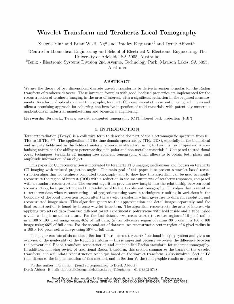
A significant characteristic of the wavelet transform is its a large number of vanishing moments. Hilbert trans-forms of functions with many vanishing moments have been shown to decay very rapidly at infinity.15 In otherwords, a wavelet function with compactly supported allows a local basis to maintain its localised features afterHilbert transformation.15 Fig. (1)(a)-(c) illustrates the ramp filter over the full frequency domain, the Bior-Splines bi-orthogonal scaling and wavelet filters and the ramp filtered version of the BiorSplines bi-orthogonalwavelet and scaling filters, where the X axis means the number of time or frequency samples, and Y axis meansthe relative amplitude. Fig. (1)(c) essentially shows the essentially compact support after applying Hilbert trans-forms. Therefore, the wavelet and scaling coefficients for some wavelet basis can be calculated after applyingthe projections passing through the region of interest plus a margin for the support of the wavelet and scalingramp filters. These reconstructed coefficients, in this experiment, are then directly applied to the inverse wavelettransforms for terahertz image reconstruction.

3. IMPLEMENTATION

3.1. Practical Consideration

The current research based on terahertz imaging is most closely related to Rashid-Farrokhi et al.14 In this work,we experiment with the 2D wavelet technique using terahertz tomographic data by modifying the measuredprojections. As we show later, this modification involves an extrapolation technique to avoid edge effects dueto sinogram truncation. It is observed that approximate coefficients of a scaling function shows good localisedfeatures in the local reconstruction using our algorithm, where the reconstructed intensity of an image variesmuch between different target materials. It should be noted that, in the application of terahertz data for localreconstruction, it is found that the intensity at the edges of the region of exposure (ROE) in terahertz projections,where nonlocal data is set to zero, varies considerably after conducting either a traditional ramp filter or scalingand wavelet ramp filters.

SPIE-OSA Vol. 6631 663113-4

50 100 150 200 2500

0.1

0.2

0.3

0.4

0.5

0.6

0.7

0.8

0.9

1ramp filter in the frequency domain

frequency bin

ampl

itude

(a.u

.)

(a)

5 10 15 20 25 30 35−0.5

0

0.5

1

1.5

scaling and wavelet filters

scaling ramp filterhorizontal wavelet ramp filtervertical wavelet ramp filterdiagonal waveletr ramp filter

time step

ampl

itude

(a.u

.)

(b)

5 10 15 20 25 30 35

−0.2

0

0.2

0.4

0.6

0.8

scaling and wavelet ramp filters

scaling ramp filterhorizontal wavelet ramp filtervertical wavelet ramp filterdiagonal waveletr ramp filter

time step

ampl

itude

(a.u

.)

(c)

Figure 1. (a) Illustration of a traditional ramp filter. (b) and (c) Illustration of the scaling and wavelet ramp filters atthe sixth projection angle (43.2 degree) using BiorSplines 2.2 wavelet, respectively.

(a) (b)

10 20 30 40 50

−40

−30

−20

−10

0

10

20

30

40

Projection profile at 25th angle

ampl

itude

(a.

u.)

projection (mm)

ramp filtered projectionwavelet ramp filtered projection

(c)

10 20 30 40 50−2

−1

0

1

2

3

4

5

6

7

Projection profile at 25th angle after Extrapolation

ampl

itude

(a.

u.)

projection (mm)

scaling ramp filtered projectionramp filtered projection

(d)

Figure 2. (a) An optical image of a target with 2 mm diameter holes drilled into a polystyrene cylinder with varyinginterhole distances. (b) Target object photograph with simple nested structure. The line indicates the measurementheight of 7 mm. (c) Projection filtered by a scaling ramp filter and a traditional ramp filter, respectively. (d) Projectionextrapolation outside the ROI after filtered projections.

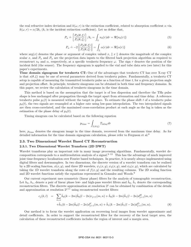
In local reconstruction, artifacts are common close to the boundary of the ROE, which can readily be observedin the application to terahertz CT data. It is possible that reconstruction after applying a constant linearextrapolation results in missing information. This situation is illustrated in subsection 4.1.3. In this paper, thereare two sets of terahertz data considered for reconstruction: a cylinder with holes inside (see the target photoin Fig 2(a)) and a nested structure of a tube inside a vial. For the first set of terahertz data (the sample photoin Fig 2(b)), with 101 projections at each of 25 projection angles covering a 180◦ projection area in a 100 × 100image. The line in the photo indicates the measurement height of 7 mm. Two situations are analyzed for thistarget sample: (i) an ROE of diameter 42 pixels at the center of the image and (ii) an ROE of diameter 67 pixelsoffcenter to the image. For the second set of terahertz measurements, with 51 projections at each of 36 projectionangles covering a 360◦ projection area in a 100 × 100 image, an ROE of diameter 18 pixels at the center of theimage is explored. Each of dataset has a pixel interval of 0.5 mm.

Fig 2(c) shows sharp variation along the borders of the ROE after applying wavelet ramp filters and rampfilter, respectively, on each of the 1D projections, which result in an image appearing relatively weakened intensitycompared to a large constant bias that exists along the reconstructed edges in the region of interest. The constantextrapolation we use is given by Eq. 25 in Rashid-Farrokhi et al.14 In order to fit terahertz signals, the currentalgorithm replaces re with (re − ra) to diminish the artificial effect along the edge of ROE, where ra is the radius

SPIE-OSA Vol. 6631 663113-5

of the region of artifacts (ROA) centered at the origin.

Fig. 2(d) shows the extrapolated projection at the 25th projection angle after the application of a scaling rampfilters and a ramp filter. The extrapolated projection removes spikes at the edge of the ROE. The extrapolationalgorithm is suitable to the reconstruction of an image at the off-center area. In order to recover the cross-sectionalimage in the region of interest, the values of the sinograms outside of the ROE are set to zero. The traditionalfiltered back projection formulas and wavelet based reconstruction are applied to the remaining projections,respectively for analysis and comparison. The original terahertz sinogram image for the current terahertz datacan be calculated via applying Eq. (6).

3.1.1. Example Three

The third experiment is performed on a simple sample with a nested structure, a tube inserted in a vial. Eq. (7) isapplied to perform a Radon transform on the measured terahertz projection data. Eq. (9) is used to reconstructa local image using a scaling ramp filter, with G2j being multiplied by a shape scaling factor λ. The Eq. (9) canbe rewritten

I(x, y) =∫ π

0

dθ ·[∫ ∞

−∞s(θ, β)|β|g2j (10)

·[β(cos θ · λ), β(sin θ · λ)]exp[i2πβξ]dβ

].

Fig 3(a) shows the wavelet ramp filtered projection at the first sampled frequency before a shape scalingfactor is applied, where a large ‘S’ shape scaling ramp filtered projection is observed. Fig 3(b) shows and almostflat border along the projection after applying a shape scaling factor of 1/3.

Num

ber

of p

roje

ctio

ns

Angle (degrees)

Scaling ramp filtered sinogram

0 50 100 150 200 250 300 350

0

5

10

15

20

25

30

35

40

45

50

0.05

0.1

0.15

0.2

0.25

0.3

0.35

0.4

0.45

0.5

(a)

‘

Num

ber

of p

roje

ctio

ns

Angle (degrees)

Scaled scaling ramp filtered sinogram

0 50 100 150 200 250 300 350

0

5

10

15

20

25

30

35

40

45

50

0.1

0.2

0.3

0.4

0.5

0.6

(b)

Num

ber

of p

roje

ctio

ns

Number of Angles

Extrapolation of scaled scaling ramp filtered sinogram

5 10 15 20 25 30 35

5

10

15

20

25

30

35

40

45

50

−0.1

0

0.1

0.2

0.3

0.4

(c)

Figure 3. (a) Scaling ramp filtered projection before a shape scaling factor is applied. (b) Scaling wavelet ramp filteredprojection after a shape scaling factor of 1/3 is applied. (c) Illustration of the resultant signogram via extrapolation ofscaling wavelet ramp filtered projection

In this example, it is observed that variation in the approximately flat border exists. In order to reduce theloss of necessary information in the ROI, different constants are adopted based on the different projection angles.Let us assume that the region of artifacts consists of two parts: ROA1 and ROA2 with the radii of ra1 andra2, and with the projection angles of ρ1 ∈ [0 : θa1] and ρ2 ∈ [0 : θa2], respectively, in an image. To overcomethe problem of edge discontinuities, truncated regions in the sinogram are extrapolated with a constant value,

SPIE-OSA Vol. 6631 663113-6

which satisfies Eq (11). Fig 3(c) shows the resultant sinogram via extrapolation of the scaling wavelet rampfiltered projection, with the same number of the projections at each projection angles being kept for conveniencein calculation of reconstructed image.

sθ local(p) =

⎧⎪⎪⎪⎪⎪⎪⎪⎪⎪⎪⎪⎪⎪⎪⎪⎪⎪⎪⎪⎪⎪⎪⎪⎪⎪⎪⎪⎪⎪⎪⎪⎪⎨⎪⎪⎪⎪⎪⎪⎪⎪⎪⎪⎪⎪⎪⎪⎪⎪⎪⎪⎪⎪⎪⎪⎪⎪⎪⎪⎪⎪⎪⎪⎪⎪⎩

sθ(p), ...if p ∈ (ROE-ROA1), and θ ∈ [0 : θa1]sθ(p), ...if p ∈ (ROE-ROA2), and θ ∈ (θa1 : θa2]sθ(r cos(θ − θ0) + (re − ra1)), ...if p ∈ [r cos(θ − θ0) + (re − ra1)], ...and θ ∈ [0 : θa1]sθ(r cos(θ − θ0) + (re − ra2)), ...if p ∈ [r cos(θ − θ0) + (re − ra2)],...and θ ∈ (θa1 : θa2]sθ(r cos(θ − θ0) − (re − ra1)), ...if p ∈ [r cos(θ − θ0) − (re − ra1)],...θ ∈ [0 : θa1]sθ(r cos(θ − θ0) − (re − ra2)), ...if p ∈ [r cos(θ − θ0) − (re − ra2)], ...θ ∈ (θa1 : θa2].

(11)

3.2. Algorithm Summary

The wavelet based reconstruction algorithm assumes an image support of radius R, and the radius of the ROIis ri. A radius re = ri + ra is exposed, where ra is the extra margin with related to radius of ROA, which isproduced by applying wavelet filters on the project data. The algorithm is summarized as follows.

3.3. Algorithm Summary

The wavelet based reconstruction algorithm assumes an image support of radius R, and the radius of the ROIis ri. A radius re = ri + ra is exposed, where ra is the extra margin with related to radius of ROA, which isproduced by applying wavelet filters on the project data. The algorithm is summarized as follows.

1. The original projections are calculated from time or frequency parameters from terahertz measurements.

2. The region of exposure is truncated for the reconstruction of an image in the region of interest.

3. The region of exposure of each projection is filtered by modified wavelet filters at all projection angles.This step is to recover an image related to wavelet detailed coefficients.

4. The region of exposure of each projection is filtered by modified scaling filter at all projection angles, whichwill lead to the recovery of the approximation sub-image.

5. The projections from step 4 are extrapolated with constants to limit artifacts at the boundaries of theprojections.

6. Filtered projections obtained in Step 3 and Step 4 are back projected to every other point to obtain theapproximate and detail at the higher resolution. The remaining points are set to zero.

7. The image is reconstructed from the wavelet and scaling coefficients via a conventional inverse DWT.

SPIE-OSA Vol. 6631 663113-7

4. RECONSTRUCTION RESULTS

4.1. Global Reconstruction

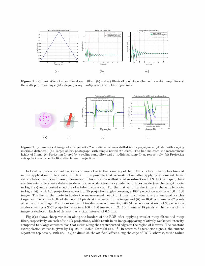
A 196×196 pixel image of the polystyrene target is recovered from the wavelet and scaling coefficients using globaldata, shown in Fig. 4(a), without decomposition in the inverse wavelet transform for clarity and comparison. Eachmeasured terahertz pulse is a function of time with 401 samples at uniform time intervals of 0.067 ps. Waveletand scaling coefficients after back projection are shown in Fig. 4(b), where the BioSpline 2.2 biorthogonal basisis used. The quality of the reconstructed image is, as expected, almost indistinguishable from the reconstructionusing traditional filtered back projection (FBP). The differences between the wavelet based reconstruction andtraditional filtered back projection are evaluated using the reconstructed profiles at the 80th horizontal row ofpixels and 80th vertical column of pixels, illustrated in Fig. 4(d) and (e), where it is not difficult to see thevariation in detected hole positions using wavelet version of reconstruction (dash line) compared to traditionalFBP algorithm (dash dot line).

0 20 40 60 80

0

10

20

30

40

50

60

70

80

X (mm)

Y (

mm

)

0.5

1

1.5

2

2.5

3

Centered wavelet based global CT

(a)

20 40 60 80 100

20

40

60

80

10020 40 60 80 100

20

40

60

80

100

20 40 60 80 100

20

40

60

80

10020 40 60 80 100

20

40

60

80

100

(b)

20 40 60 80 100 120 140 160

0

0.5

1

1.5

2

2.5

Reconstructed profile at 80th horizontal pixel row

FBPWT based recon.

Mag

nitu

de (

dB)

Number of pixels

(c)

20 40 60 80 100 120 140 160

0

0.5

1

1.5

2

2.5

Reconstructed profile at 80th vertical pixel column

FBPWT based recon.

Number of pixels

Mag

nitu

de (

dB)

(d)

Figure 4. (a) A 196 × 196 pixel image of the polystyrene target is recovered from the wavelet and scaling coefficientsusing global data, without decomposition. (b) Wavelet and scaling coefficients after back projection. (c) Reconstructedprofiles at the 80th horizontal pixel row. (d) Reconstructed profiles at the 80th vertical pixels column.

4.2. Local Reconstruction at Center Area

Wavelet Based Tomography

Y (

mm

)

X (mm)0 20 40 60 80

0

10

20

30

40

50

60

70

80

90 1

1.5

2

2.5

3

3.5

4

4.5

5

(a)

Y (

mm

)

X (mm)

0 20 40

0

10

20

30

40

50

Y (

mm

)

X (mm)0 20 40

0

10

20

30

40

50

Y (

mm

)

X (mm)0 20 40

0

10

20

30

40

50

Y (

mm

)

X (mm)0 20 40

0

10

20

30

40

50

(b)

5 10 15 20 252

2.5

3

3.5

4

4.5

5

5.5

6

6.5

Reconstructed profile at 12th horizontal pixel row

Mag

nitu

de (

dB)

Number of pixels

scaling ramp filtered LCTramp filtered GCTramp filtered LCTwavelet based LCT

(c)

5 10 15 20 251

1.5

2

2.5

3

3.5

4

4.5

5

5.5

6

Reconstructed profile at 12th vertical pixel column

Mag

nitu

de (

dB)

Number of pixels

scaling ramp filtered LCTramp filtered GCTramp filtered LCTwavelet based LCT

(d)

Figure 5. (a) Reconstructed image localised to a region of interest from the inverse wavelet transform. (b) Centeredapproximate and three detail reconstruction subimages along clockwise direction. (c) Reconstructed profiles at the 12thhorizontal pixel row. (d) Reconstructed profiles at the 12th vertical pixel column.

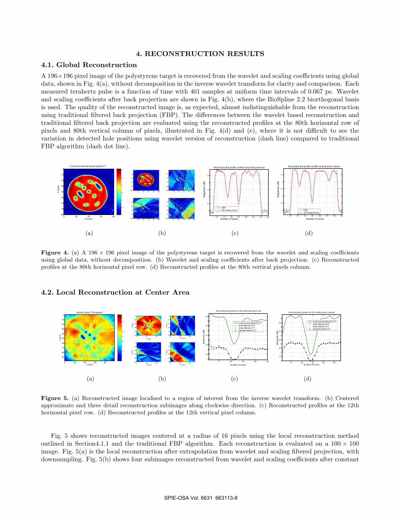
Fig. 5 shows reconstructed images centered at a radius of 16 pixels using the local reconstruction methodoutlined in Section4.1.1 and the traditional FBP algorithm. Each reconstruction is evaluated on a 100 × 100image. Fig. 5(a) is the local reconstruction after extrapolation from wavelet and scaling filtered projection, withdownsampling. Fig. 5(b) shows four subimages reconstructed from wavelet and scaling coefficients after constant

SPIE-OSA Vol. 6631 663113-8

extrapolation and BP. Fig. 5(c) and (d) shows the reconstruction profiles at the 12th horizontal row and verticalcolumn of pixels corresponding to each reconstruction. As illustrated in Fig. 5(c) and (d), the profiles taken fromthe image reconstruction are scaled to improve construct.

4.3. Local Reconstruction at off-Center AreaFig. 6(a)-(d) shows reconstructed images at an off-center area with a radius of 61 pixels using the current localreconstruction method and the traditional FBP algorithm. Each of the subfigures illustrates, for comparison, localreconstruction from extrapolated wavelet and scaling filtered projection after decomposition; the reconstructionof extrapolated approximate and detail coefficients after BP; the reconstruction profiles at the 28th horizontalrow of pixels and the 12th vertical column of pixels are illustrated in Fig. 6(c) and (d), both of which correspondto the reconstructions from approximate wavelet coefficients, FBP based local and global recovery in the ROI.The reconstruction from wavelet approximate coefficients shows strong contrast in intensity for different mediaand FBP based local reconstruction shows a little higher intensity than FBP based global reconstruction.

Extrapolated wavelet based LCT

Y (

mm

)

X (mm)0 20 40 60 80

0

10

20

30

40

50

60

70

80

90 0.5

1

1.5

2

2.5

3

3.5

4

4.5

5

(a)

Y (

mm

)

X (mm)0 20 40

0

10

20

30

40

50

Y (

mm

)

X (mm)0 20 40

0

10

20

30

40

50

Y (

mm

)

X (mm)0 20 40

0

10

20

30

40

50

Y (

mm

)

X (mm)0 20 40

0

10

20

30

40

50

(b)

5 10 15 201

1.5

2

2.5

3

3.5

4

4.5

5

5.5

6

Reconstructed profile at 28th horizontal pixel row

Mag

nitu

de (

dB)

Number of pixels

scaling ramp filted LCTramp filtered LCTramp filtered GCT

(c)

10 20 30 40 50 60

0

1

2

3

4

5

6

7

8

Reconstructed profile at 12th vertical pixel column

Mag

nitu

de (

dB)

Number of pixels

scaling ramp filted LCTramp filtered LCTramp filtered GCT

(d)

Figure 6. (a) A reconstructed image from the inverse wavelet transform without decomposition for clarity. (b) Off-centered approximate and three detail reconstructed subimages along clockwise direction. (c) Reconstructed profiles atthe 28th horizontal row of pixels. (d) Reconstructed profiles at the 12th vertical column of pixels.

4.4. Example ThreeThe nested structure of a tube inside a PET vial is imaged on a 100×100 grid. Its reconstruction from the waveletand scaling coefficients using global data is shown in Fig. 7(a). The ten images span the sampled frequency scopefrom ten lowest frequencies, from 0.0213 THz to 0.213 THz. Again, the BioSpline 2.2 biorthogonal basis isused. The quality of the reconstructed image is similar to using traditional filtered back projection (FBP),shown in Fig. 7(b), with a little increased recovered image intensity in the reconstructed subimages and a littlediscontinuity in the third reconstructed subimage compared to the traditional FBP algorithm.

Fig. 7(c) and (d) shows reconstructed images after extrapolation, evaluated on a 100×100 grid, at a center areawith a disk radius of 6 pixels using the current local reconstruction method and the traditional FBP algorithm.They are enlarged for clarity. Each of the reconstructed subimages is illustrated, from 0.0213 THz to 0.213 THz,relatively, with 59% of full projection data. The 59% of full projections is shown in Fig. 7(e) at the 6th sampledfrequency. The local reconstruction in the ROI from extrapolated wavelet and scaling filtered projection is shownin Fig. 7(c). Fig. 7(d) is the corresponding local reconstructions using FBP algorithm. The noise is obviouslyreduced in wavelet based reconstructed images, especially at the two frequencies of 0.0213 THz and 0.0426 THz.It is valuable in the exploration of biomedical images using terahertz data, though a little aliasing occurs. Thewavelet approximate and detailed coefficients after BP at the 7th sampled frequency is illustrated in Fig. 7(f),with a relative error of 29% from the approximate reconstruction.

5. FUTURE WORK

Since the current work involves only the one level of 2D DWT, it is interesting to explore the reconstruction algo-rithm with more levels of decomposition. Moreover, a research area of much current interest is the development

SPIE-OSA Vol. 6631 663113-9

¶ —

0.1

0.2

0.3

0.4

0.5

0.6

Global FBP

(a)

0.05

0.1

0.15

0.2

0.25

0.3

Global wavelet based reconstruction

(b)

0.05

0.1

0.15

0.2

0.25

0.3

0.35

wavelet based LCT

(c)

0.1

0.2

0.3

0.4

0.5

0.6

FBP based LCT

(d)

Num

ber o

f pro

ject

ion

Number of angles

59% truncated sinogram

0 5 10 15 20 25 30 35

0

5

10

15

20

25

30

35

40

45

50

(e) (f)

Figure 7. (a) Illustration of a 100×100 pixel global image of the tube inside a vial, with frequency range from 0.0213 THzto 0.213 THz. It is recovered from the wavelet and scaling coefficients, after decomposition. (b) FBP based reconstructionfrom global measurement with size of 100× 100 pixels and the same frequency range of (a). (c) A reconstructed image ofthe tube from the inverse wavelet transform after decompostion. (d) Corresponding reconstruction FBP algorithm usinglocal projection data. (e) Illustration of the truncated projections with 59% of full data. (f) Approximate and detailreconstruction coefficients after BP using local projection data.

SPIE-OSA Vol. 6631 663113-10

of statistical based local tomography algorithm and techniques.16 It aims towards the actual localised recon-struction with relation to the terahertz measurement. The wavelet technique is critical for local reconstruction,and the relative wavelet transform coefficients can be thresholded to reduce the dimensions of the computationalproblem.17 In addition, the current resultant experiment relies on the fact that the Hilbert transform (part ofthe inverse RT) does not really change the compact support of scaling and wavelet functions. Selesnick in hispaper18 pointed out how to design coupled sets of scaling and wavelet functions which are approximate Hilberttransforms of each other. This could prove to be useful in the future work.

6. CONCLUSIONWe have developed an algorithm to reconstruct the wavelet and scaling coefficients of a function from its signo-gram image of terahertz signals. Based on the observation that for some wavelet bases, with sufficient zeromoments, the scaling and wavelet functions have essentially the same support after ramp filtering. Two targetsare recovered from terahertz measurements, which demonstrates the current local reconstruction reconstructionmethod using a wavelet based transform scheme.

REFERENCES1. K. L. Nguyen, M. L. Johns, L. Gladden, C. H. Worrall, P. Alexander, H. E. Beere, M. Pepper, D. A.

Ritchie, J. Alton, S. Barbieri, and E. H. Linfield, “Three-dimensional imaging with a terahertz quantumcascade laser,” Optics Express 14(6), pp. 2123–2129, 2006.

2. P. S. Carney, E. Wolf, and G. S. Agarwal, “Diffraction tomography using power extinction measurements,”Journal of the Optical Society of America A: (Optics & Vision) 16(11), pp. 2643–2648, 2002.

3. T. D. Dorney, W. W. Symes, R. G. Baraniuk, and D. M. Mittleman, “Terahertz multistatic reflectionimaging,” Journal of the Optical Society of America A 19, pp. 1432–1442, 2002.

4. S. Wang, B. Ferguson, and X.-C. Zhang, “Pulsed terahertz tomography,” Journal of Physics D: AppliedPhysics 37, pp. R1–R36, (See also Erratum: Journal of Physics D : Applied Physics, 37, p. 964, 2004.),2004.

5. A. B. Ruffin, J. Van Rudd, J. Decker, L. Sanchez-Palencia, L. Le Hors, J. F. Whitaker, and T. B. Norris,“Time reversal terahertz imaging,” IEEE Journal of Quantum Electronics 38(8), pp. 1110–1119, 2002.

6. X.-X. Yin, B. W.-H. Ng, B. Ferguson, S. P. Mickan, and D. Abbott, “2-d wavelet segmentation in 3-d t-raytomography,” IEEE Sensors Journal 7(3), pp. 342–343, 2007.

7. B. Ferguson, S. Wang, D. Gray, D. Abbott, and X. Zhang, “Toward functional 3D T-ray imaging,” Physicsin Medicine and Biology (IOP) 47, pp. 3735–3742, 2002.

8. B. Ferguson, S. Wang, D. Gray, D. Abbott, and X. C. Zhang, “Identification of biological tissue using chirpedprobe THz imaging,” Microelectronics Journal (Elsevier) 33(12), pp. 1043–1051, 2002.

9. R. C. Gonzalez and R. E. Woods, Digital Image Processing, Prentice-Hall, Inc., New Jersey, 2002.10. S. Mallat, A Wavelet Tour of Signal Processing, Academic Press, San Diego, CA., 1999.11. I. Daubechies, Ten Lectures on Wavelets, Society for Industrial and Applied Mathematics (SIAM), Philadel-

phia, PA, 1992.12. A. Jensen and A. la Cour-Harbo, Ripples in Mathematics: The Discrete Wavelet Transform, Springer Verlag,

Berlin, 2001.13. D. Percival and A. Walden, Wavelet Methods for Time Series Analysis, Cambridge University Press, Cam-

bridge, England, 2000.14. F. Rashid-Farrokhi, K. Liu, C. Berenstein, and D. Walnut, “Wavelet-based multiresolution local tomogra-

phy,” IEEE Transactions on Image Processing 6(10), pp. 1412–1430, 1997.15. A. H. Delaney and Y. Bresler, “Multiresolution tomographic reconstruction using wavelets,” IEEE Transac-

tions on Image Processing 4(6), pp. 799–813, 1995.16. K. M. Hanson and G. W. Wecksung, “Bayesian estimation of 3-D objects from few radiographs,” Journal of

Optical Society of America 73(11), pp. 1501–1509, 1983.17. A. Meyer-Baese, Pattern Recognition in Medical Imaging, Academic Press, Inc., Orlando, FL, USA, 2003.18. I. W. Selesnick, “The design of approximate Hilbert transform pairs of wavelet bases,” IEEE Transactions

on Signal Processing 50(5), pp. 1144–1152, 2002.

SPIE-OSA Vol. 6631 663113-11