Wavelets and Multiscale Edge Detection

Brody Dylan Johnson

Saint Louis University

1

Abstract:In 1992, Mallat and Zhong published a paper presenting a numer-ical technique for the characterization of one- and two-dimensionaldiscrete signals in terms of their multiscale edges [2]. With the appro-priate choice of wavelet, the locations of edges correspond to modulusmaxima of the continuous wavelet transform at a given scale. In thistalk, we will explore the fundamentals of the Mallat-Zhong approach.

2

Overview:• 1-D Edge Detection and Signal Characterization

– smoothing functions and “wavelet derivatives”

– stability of continuous wavelet transform

– practical considerations

– example

• 2-D Edge Detection

– Canny edge detector

– examples

3

The smoothing function:• We say θ(x) is a smoothing function if θ ∈ C2(R), has a

fast decay (so that θ is C2), and∫R θ(x) = 1. Under these

assumptions, θ ∈ Lp(R), 1 ≤ p ≤ ∞.

• Prototypical example: the Gaussian, θ(x) = 1√πe−x2

.

• At scale s > 0, we have a dilated version of the smoothing func-

tion, θs(x) :=1sθ(

x

s), which also satisfies

∫R θs(x) = 1.

• For f ∈ L2(R), the convolution (f ∗ θs)(x) is a smoothed versionof f (twice-differentiable) at the scale s > 0. Moreover,

lims→0

(f ∗ θs)(x) = f(x) a.e..

• Interpretation: (f ∗ θs) removes variation from f that occurs atresolutions finer than s.

4

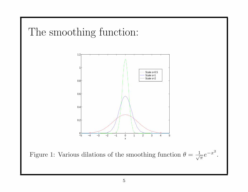
The smoothing function:

Scale s=0.5Scale s=1 Scale s=2

−5 −4 −3 −2 −1 0 1 2 3 4 50

0.2

0.4

0.6

0.8

1

1.2

x

Figure 1: Various dilations of the smoothing function θ = 1√πe−x2

.

5

The Fourier transform:• The Fourier transform of f ∈ L1 ∩ L2(R) is defined by

Ff(ξ) = f(ξ) =∫

Rf(x)e−2πix·ξdx.

• Relevant properties of the Fourier transform:

1. (Ff ′(x))(ξ) = (2πiξ)f(ξ)

2. (Fxf(x))(ξ) = i2π f ′(ξ)

3. f(0) =∫

Rf(x)dx

• The Parseval formula for f, g ∈ L1 ∩ L2(R):

〈f, g〉 =∫

Rf(x)g(x)dx =

∫

Rf(ξ)g(ξ)dξ = 〈f , g〉.

6

The wavelets:• Given a smoothing function θ as above, define

ψa(x) =dθ

dx(x) & ψb(x) =

d2θ

dx2(x).

• ψa and ψb are wavelets in the sense that∫

Rψa(x)dx =

∫

Rψb(x)dx = 0.

This is because ψa(ξ) = (2πiξ)θ(ξ), ψb(ξ) = (2πiξ)2θ(ξ), andθ(0) = 1, implying ψa(0) = ψb(0) = 0.

7

The wavelets:

−5 −4 −3 −2 −1 0 1 2 3 4 5−1.5

−1

−0.5

0

0.5

1

x

(b)

−5 −4 −3 −2 −1 0 1 2 3 4 5−0.5

0

0.5(a)

Figure 2: The wavelets: (a) ψa and (b) ψb associated with thesmoothing function θ = 1√

πe−x2

. The wavelet ψb is often referred toas the Mexican hat function.

8

Continuous wavelet transform:• The continuous wavelet transforms defined by ψa and ψb, re-

spectively, are

W as f(x) = (f ∗ ψa

s )(x) = sd

dx(f ∗ θs)(x)

and

W bs f(x) = (f ∗ ψb

s)(x) = s2 d2

dx2(f ∗ θs)(x).

• W as f measures the derivative of the smoothed version of a signal

f at scale s, while W bs f measures the second derivative.

• Wavelets work by translation and dilation:

W as f(x) =

∫

Rf(y)ψa

s (x− y)dy = 〈f, Txψas 〉,

i.e., W as f(x) is an inner product with a translation and dilation

of ψas . (The involution of f is f , given by f(x) = f(−x).)

9

Defining edges:• An edge should correspond to a point where f(x) undergoes

rapid variation, i.e., maxima of f ′(x). We cannot investigatef ′(x) directly, but we can instead study W a

s f(x).

• Loosely speaking, we will say that f(x) has an edge at x = a ifWsf(x) has a local maxima at x = a. (x = a should remain alocal maxima as s → 0)

• The local extrema of W as f(x) correspond to the zero crossings

of W bs f(x) and the inflection points of (f ∗ θs)(x).

• Thus, W as and W b

s can each be used to locate eges, but thezero crossings of W b

s f fail to separate between the local maximaand minima of f . The minima of W b

s f correspond to points ofsmooth variation of f and will not give rise to edges.

10

Achieving a stable representation:• Mallat and Zhong want to use the modulus maxima of W a

s f toreconstruct f , but it is not even obvious that one can reconstructf from W a

s f .

• Instead of consdering all scales s > 0 we will consider only dyadicscales 2j , j ∈ Z.

• Assume that ψ satisfies a Calderon inequality:

A ≤∑

j∈Z|ψ(2jξ)|2 ≤ B a.e. ξ ∈ R.

• Define the Dyadic Wavelet Transform: Wψ : L2(R) → L2(Z,R),f 7→ {Wψ

2j f}j∈Z, where

W2j f := Wψ2j f = (f ∗ ψ2j )(x).

11

Completeness of the wavelet transform:

Claim: A‖f‖2 ≤∑

j∈Z‖W2j f‖2 ≤ B‖f‖2.

Proof: Observe that∑

j∈Z‖W2j f‖2 =

∑

j∈Z

∫

R|W2j f(x)|2 dx

(Parseval) =∑

j∈Z

∫

R|f(ξ)|2|ψ2j (ξ)|2 dξ

=∑

j∈Z

∫

R|f(ξ)|2|ψ(2jξ)|2 dξ

=∫

R|f(ξ)|2

( ∑

j∈Z|ψ(2jξ)|2

)dξ.

12

Reconstruction:• Suppose we find χ(x) so that

∑

j∈Zψ(2jξ)χ(2jξ) = 1,

then we can recover f from W2j f via

f(x) =∑

j∈Z

(W2j f ∗ χ2j

)(x).

• This follows from the Fourier transform:∑

j∈Zf(ξ) ψ(2jξ) χ(2jξ) = f(ξ)

∑

j∈Zψ(2jξ) χ(2jξ) = f(ξ).

• Reconstruction from modulus maxima is another story, however,which will be addressed briefly below.

13

Practical considerations:• In practice one encounters discretely defined functions, not func-

tions of a continuous variable. Hence, we need a discrete versionof the continuous wavelet transform.

• Let θ, ψ, and χ be refinable, i.e., there exists m0,m1,m2 ∈L∞(T) such that

θ(2ξ) = m0(ξ)θ(ξ), ψ(2ξ) = m1(ξ)θ(ξ), and χ(2ξ) = m2(ξ)θ(ξ)

with the additional assumption (perfect reconstruction condi-tion) that

|m0(ξ)|2 + m1(ξ)m2(ξ) = 1.

• We now replace the continuous wavelet transform with a discretewavelet transform known as the a trous algorithm.

14

The a trous algorithm:• The refinability of the smoothing function and wavelets provides

useful relationships between the values of the wavelet transformacross scales:

〈f, Tkθ2j−1〉 =∑

`∈Zα`〈f, Tk+2j`θ2j 〉,

and〈f, Tkψ2j−1〉 =

∑

`∈Zβ`〈f, Tk+2j`θ2j 〉,

where m0(ξ) =∑

`∈Z α`e−2πi`ξ and m1(ξ) =

∑`∈Z β`e

−2πi`ξ.

• The a trous algorithm uses these relationships to compute f ∗θ2j−1 and W2j−1f from f ∗θ2j . In practice a signal is interpretedas f ∗ θ20 in this algorithm. Reconstruction is similar.

15

Reconstruction from modulus maxima:• A frame for a Hilbert space H is a collection {xj}j∈J for which

there exists 0 < A ≤ B < ∞ so that for each x ∈ H

A‖x‖2 ≤∑

j∈J|〈x, xj〉|2 ≤ B‖x‖2.

• The reconstruction described above amounts to the existence ofa dual frame {yj}j which for each x ∈ H satisfies

x =∑

j∈J〈x, xj〉yj .

• By considering only modulus maxima in reconstruction we areattempting to recover x using only {〈x, xjk

〉} for some subse-quence {jk} ⊂ J.

16

Reconstruction from modulus maxima:• It has been shown that different functions can have the same

modulus maxima (see [1] for references), but these signals tend tobe very similar and for this reason fairly accurate reconstructionsare possible using modulus maxima.

• A dual frame can no longer be used for reconstruction. Instead,the original function is recovered using the frame algorithm,which is an iterative algorithm for inverting the partial frameoperator [1].

• The frame operator associated to {xj} is defined by

Sx =∑

j∈J〈x, xj〉xj .

17

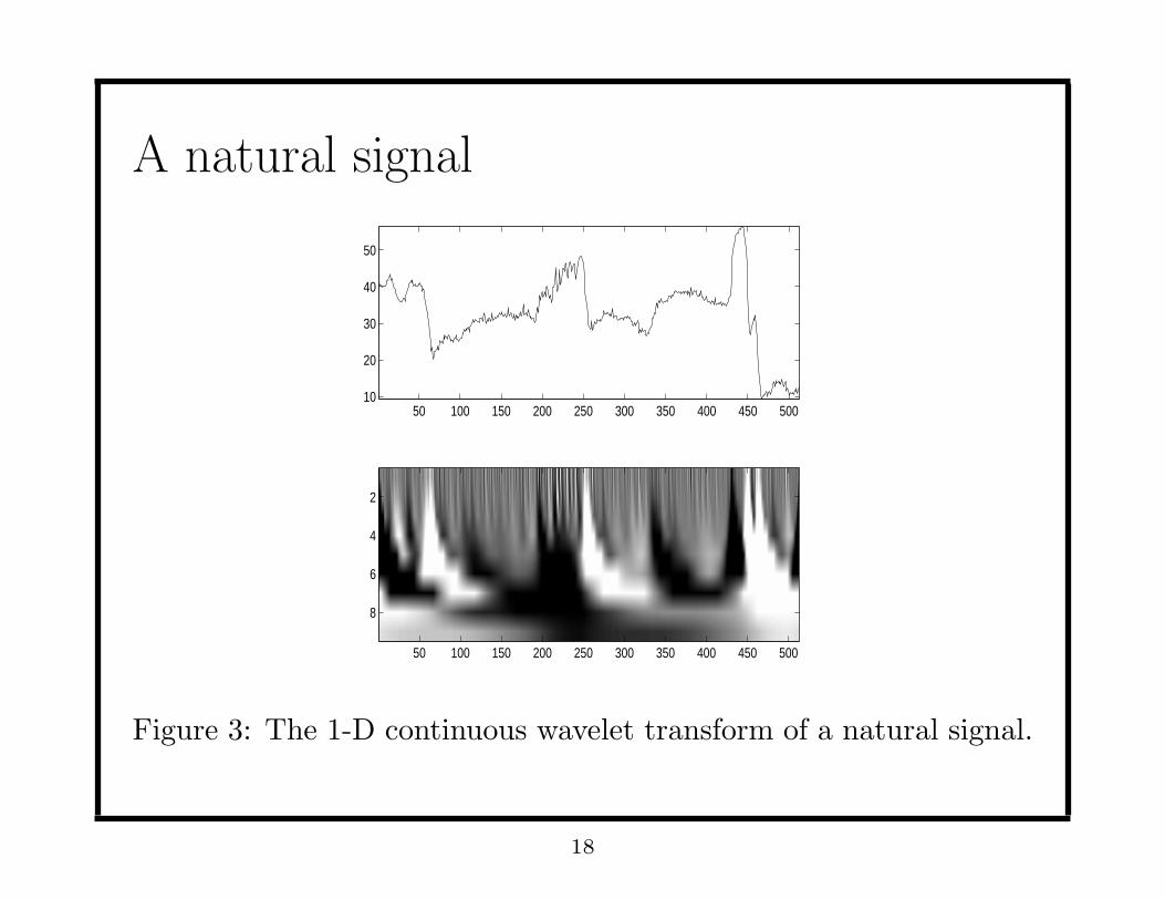
A natural signal

50 100 150 200 250 300 350 400 450 50010

20

30

40

50

50 100 150 200 250 300 350 400 450 500

2

4

6

8

Figure 3: The 1-D continuous wavelet transform of a natural signal.

18

Smoothing across scales:

100 200 300 400 500

20

40

Scale: −1

100 200 300 400 500

20

40

Scale: −2

100 200 300 400 500

20

40

Scale: −3

100 200 300 400 500

20

40

Scale: −4

100 200 300 400 500

20

40

Scale: −5

100 200 300 400 500

20

40

Scale: −6

100 200 300 400 500

20

40

Scale: −7

100 200 300 400 500

20

40

Scale: −8

Figure 4: The smoothed versions of the signal at various scales.

19

Modulus of the wavelet transform:

100 200 300 400 5000

50

Scale: −1

100 200 300 400 5000

20

40

Scale: −2

100 200 300 400 5000

20

40

Scale: −3

100 200 300 400 5000

20

40

Scale: −4

100 200 300 400 5000

50Scale: −5

100 200 300 400 5000

50Scale: −6

100 200 300 400 5000

20

Scale: −7

100 200 300 400 5000

5

10

Scale: −8

Figure 5: The modulus of the continuous wavelet transform at vari-ous scales.

20

Modulus maxima:

100 200 300 400 5000

50

Scale: −1

100 200 300 400 5000

20

40

Scale: −2

100 200 300 400 5000

20

40

Scale: −3

100 200 300 400 5000

20

40

Scale: −4

100 200 300 400 5000

50Scale: −5

100 200 300 400 5000

50Scale: −6

100 200 300 400 5000

20

Scale: −7

100 200 300 400 5000

5

10

Scale: −8

Figure 6: The modulus maxima of the continuous wavelet transformat various scales.

21

Reconstruction from modulus maxima:

original reconstructed

0 50 100 150 200 250 300 350 400 450 5000

10

20

30

40

50

Figure 7: The comparison of the original signal and the signal re-constructed from the modulus maxima.

22

Two-dimensions:• Smoothing function: θ(x, y) = θ(x)θ(y), where θ is a 1-D smooth-

ing function.

• Define two wavelets: ψ1(x, y) := ∂∂x θ(x, y) = ψa(x)θ(y) and

ψ1(x, y) := ∂∂y θ(x, y) = θ(x)ψa(y), where ψa(x) = d

dxθ(x).

• Let ψ1s(x, y) = 1

s2 ψ1(xs , y

s ) and ψ2s(x, y) = 1

s2 ψ2(xs , y

s ) and fors = 2j , j ∈ Z, consider the dyadic wavelet transforms:

W 1s f(x, y) = (f ∗ ψ1

s)(x, y) and W 2s f(x, y) = (f ∗ ψ2

s)(x, y).

• If χ1(x, y) and χ2(x, y) satisfy:∑

j∈Zψ1(ξ1, ξ2)χ1(ξ1, ξ2) + ψ2(ξ1, ξ2)χ2(ξ1, ξ2) = 1,

then the two-dimensional wavelet transform will allow recon-struction as above.

23

The Canny edge detector:• Observe that

W 1

s f(x, y)

W 2s f(x, y)

= s

∂∂x (f ∗ θs)(x, y)∂∂y (f ∗ θs)(x, y)

= s∇(f ∗ θs)(x, y).

• The Canny algorithm defines (x0, y0) to belong to an edge if‖∇f(x, y)‖ is locally maximum at (x0, y0) in the direction of∇f(x0, y0).

• According to [1], it remains an open problem as to whether ornot such edges yield a complete and stable representation in twodimensions. The algorithm of [2] does provide numerical supportfor this hypothesis.

24

A natural image:

A snow leopard from the St. Louis Zoo.

25

Scale s = −1:

∂f∂x

∂f∂y

‖∇f‖ Modulus Maxima

26

The modulus of the wavelet transform:

27

Modulus maxima: scale = -2

28

Modulus maxima: scale = -3

29

Modulus maxima: scale = -4

30

Modulus maxima: scale = -5

31

Reconstructed image:

(Some “small” modulus maxima were ignored in reconstruction.)

32

Original image:

33

Monarch example:

34

Mandrill example:

35

Lena example:

36

References

[1] Stephane Mallat. A wavelet tour of signal processing. Associated Press,

1998.

[2] Stephane Mallat and Sifen Zhong. Characterization of signals

from multiscale edges. IEEE Trans. Patt. Anal. and Mach. Intell.,

14(7):710–732, 1992.

37