waves in high-speed plasmoids in the magnetosheath and at

Ann. Geophys., 32, 991–1009, 2014www.ann-geophys.net/32/991/2014/doi:10.5194/angeo-32-991-2014© Author(s) 2014. CC Attribution 3.0 License.

Waves in high-speed plasmoids in the magnetosheathand at the magnetopause

H. Gunell1, G. Stenberg Wieser2, M. Mella3, R. Maggiolo1, H. Nilsson2, F. Darrouzet1, M. Hamrin 4, T. Karlsson5,N. Brenning5, J. De Keyser1, M. André3, and I. Dandouras6

1Belgian Institute for Space Aeronomy, Avenue Circulaire 3, 1180 Brussels, Belgium2Swedish Institute of Space Physics (IRF), P.O. Box 812, 981 28 Kiruna, Sweden3Swedish Institute of Space Physics (IRF), Box 537, 751 21 Uppsala, Sweden4Department of Physics, Umeå University, 901 87 Umeå, Sweden5Space and Plasma Physics, Royal Institute of Technology (KTH), 100 44 Stockholm, Sweden6Institut de Recherche en Astrophysique et Planétologie, UPS-CNRS, 31028 Toulouse, France

Correspondence to:H. Gunell ([email protected])

Received: 29 March 2014 – Revised: 16 June 2014 – Accepted: 11 July 2014 – Published: 22 August 2014

Abstract. Plasmoids, defined here as plasma entities with ahigher anti-sunward velocity component than the surround-ing plasma, have been observed in the magnetosheath in re-cent years. During the month of March 2007 the Clusterspacecraft crossed the magnetopause near the subsolar point13 times. Plasmoids with larger velocities than the surround-ing magnetosheath were found on seven of these 13 occa-sions. The plasmoids approach the magnetopause and inter-act with it. Both whistler mode waves and waves in the lowerhybrid frequency range appear in these plasmoids, and theenergy density of the waves inside the plasmoids is higherthan the average wave energy density in the magnetosheath.When the spacecraft are in the magnetosphere, Alfvénicwaves are observed. Cold ions of ionospheric origin are seenin connection with these waves, when the wave electric andmagnetic fields combine with the Earth’s dc magnetic fieldto yield anE ×B/B2 drift speed that is large enough to givethe ions energies above the detection threshold.

Keywords. Magnetospheric physics (magnetopause, cusp,and boundary layers; magnetosheath) – space plasma physics(wave–particle interactions)

1 Introduction

The Earth’s magnetosheath is at times a highly structured re-gion, where plasma entities, distinct from the surroundingplasma by either a higher velocity or density or both, have

been observed in several studies in the last decade. A fewdifferent terms have been used in the literature to denotethese plasma entities: for example they were called “MS-jets” by Savin et al.(2005), “jets” by Hietala et al.(2009),“supermagnetosonic plasma streams” bySavin et al.(2012),“dynamic pressure enhancements” byArcher and Horbury(2013) and “plasmoids” byKarlsson et al.(2012). We shalluse the term “plasmoid” for a plasma entity with higher ve-locity than the surrounding plasma. This is different fromthe original usage (Bostick, 1956), but fits within the broaderdefinition “a coherent mass of plasma” in the Oxford EnglishDictionary (Simpson and Weiner, 1989).

High energy density jets have been observed in the mag-netosheath and shown to be deflected towards the magne-topause (Savin et al., 2008). Magnetopause deformation bysupermagnetosonic plasma streams has also been reported(Savin et al., 2011). Savin et al.(2012) observed that someof the jets appear in connection with hot flow anomalies,and that there is a significant contribution from supermagne-tosonic jets to plasma transport across magnetic boundaries.

Hietala et al.(2009) observed jets in the magnetosheathduring a period when the interplanetary magnetic field (IMF)was directed outward from the sun. These jets had speeds afew times above that of the ambient magnetosheath plasma,and it was suggested that their place of origin is at the bowshock.Hietala et al.(2012) expanded these observations andstudied their influence on ionospheric convection, and theysuggested that local ionospheric flow enhancements were

Published by Copernicus Publications on behalf of the European Geosciences Union.

992 H. Gunell et al.: Waves and plasmoids

caused by plasmoid impact on the magnetopause.Karlssonet al. (2012) studied 56 plasmoids in the magnetosheath,where each had a maximum density at least 50 % above thedensity of the surrounding plasma. A statistical study of sev-eral thousand jets confirmed that these occur during periodswith low IMF cone angles – that is to say, when the bowshock is a quasi-parallel shock (Plaschke et al., 2013b) – andshowed no significant correlation with other solar wind pa-rameters. Similar results were obtained in another statisticalstudy (Archer and Horbury, 2013).

Hietala and Plaschke(2013) used a model of a magneto-hydrodynamic shock to show that ripples on a quasi-parallelbow shock can account for the vast majority of the observedjets, and that other explanations, such as discontinuities in thesolar wind, are required only in a few percent of the observedcases.

Shue et al.(2009) observed both sunward and anti-sunward flows in the magnetosheath near the magnetopause,and it was interpreted as a jet causing an indentation on themagnetopause, which, rebounding, turned the flow back inthe sunward direction.Amata et al.(2011) found jets in themagnetosheath making indentations on the magnetopausesunward of the northern cusp.Shue and Chao(2013) showedthat a decrease in the magnetic pressure on the inside of themagnetopause is insufficient to explain the inward motionof that boundary and that instead an increased total pressureon the magnetosheath side is required.Gunell et al.(2012)used data from two of the Cluster spacecraft to show thatplasmoids, coming from the magnetosheath, penetrated themagnetopause, thus entering the magnetosphere on an occa-sion when the magnetopause motion was very slow. Mag-netopause compression and penetration of magnetosheathplasma into the magnetosphere was found byDmitriev andSuvorova(2012). The role of three-wave cascades and tur-bulence in connection with jets and plasma transport at themagnetopause was studied bySavin et al.(2014).

A theory for plasmoids penetrating magnetic barriers waspublished bySchmidt(1960); it was suggested as a processby which plasma can penetrate the dayside magnetopause byLemaire(1977); and it has been studied in both laboratoryexperiments and simulations in the last half century (see forexampleWessel et al., 1988; Hurtig et al., 2004; Brenninget al., 2005; Gunell et al., 2008, 2009; Plechaty et al., 2013).Waves, particularly in the lower hybrid frequency range, arereported in those studies, both in the laboratory and in sim-ulations. Such waves have also been observed at the mag-netopause (André et al., 2001). Also whistler mode waveshave been observed in this part of space, and such waves havebeen studied extensively in space and laboratory plasmas; seeStenzel(1999) for a review andStenberg et al.(2007), Ten-erani et al.(2013), Watt et al.(2013), Stenzel et al.(2008),or Thuecks et al.(2012) for a few examples of more recentwork. Waves are of particular interest in plasma physics, asit is through waves that energy is transferred when discreteparticle effects are negligible as a result of Debye shielding.

Furthermore, waves can cause diffusion in collisionless plas-mas leading to plasma transport across magnetic fields andto magnetic reconnection (Gekelman and Pfister, 1988).

The generation of Alfvén waves in the magnetosphere bymodulation of the solar wind dynamic pressure was studiedusing a magnetohydrodynamic model (Lysak et al., 1994).The response of the magnetosphere to pressure pulses at themagnetopause was shown to have a low-pass filtering effect(Archer et al., 2013), resulting in magnetospheric oscillationson timescales longer than the duration of any individual plas-moid impact at the magnetopause. The impact of a plasmoidon the magnetopause could alternatively be seen as a wavepulse causing a localised perturbation of that boundary. Thetransmission of waves from the magnetosheath into the mag-netosphere was examined byDe Keyser et al.(1999) andDeKeyser(2000). Waves enable the transport of energy acrossthe magnetopause, where it can be absorbed in resonant ab-sorption layers (De Keyser andCadež, 2001a), and enhancedwave amplitudes at the magnetopause can promote diffusivemass transport (De Keyser andCadež, 2001b).

Plasmoids impacting on the magnetopause cause thatboundary to move, and this will also move the plasma in thepart of the magnetosphere that is close to the impact site.Sauvaud et al.(2001) observed cold ion populations nearthe magnetopause. These ions were accelerated by anE ×B

drift, which made them visible to the ion spectrometer. Oth-erwise they are often hidden in the magnetosphere, becausetheir energy is below the threshold for detection. In the pres-ence of Alfvén waves, anE×B drift in the fields of the wavecan bring them to energies above that threshold. Convectionand magnetosonic waves can have a similar effect. Hiddencold ion populations can become visible deep in the magne-tosphere as a consequence of plasmoids in the magnetosheaththat collide with the magnetopause.André et al.(2010) foundlow-energy ion populations at the magnetopause.André andCully (2012) surveyed a large part of the magnetosphere, de-tecting cold (eV) ions in many places, and hypothesised thatthese are an important part in the escape of ions from theEarth and other planets.

In this work, we examine Cluster data from the month ofMarch 2007. During that month the outbound leg of the Clus-ter orbit crossed the magnetopause close to the subsolar pointon 13 occasions. We find plasmoids with larger velocitiesthan the surrounding magnetosheath approaching the mag-netopause from the direction of the bow shock on about halfof those days. Section2 describes how the complete data setis searched for plasmoids, and these are identified and tab-ulated. The spatial extent of the plasmoids is determined inSect.3. In Sect.4 we examine in more detail two plasmoidsthat were detected by Cluster 1 on 15 March 2007. One ofthese was observed at the magnetopause and the other in themagnetosheath. We report on the properties of waves insidethese plasmoids, and on cold ions that were seen in the mag-netosphere immediately after the plasmoid was detected bythe spacecraft. In Sect.5 it is shown that the energy density

Ann. Geophys., 32, 991–1009, 2014 www.ann-geophys.net/32/991/2014/

H. Gunell et al.: Waves and plasmoids 993

x

C3,4

C1

C2

11:00

MP

09:00

07:0005:0004:00

z

y

05:00

07:00

09:00

11:00C1

C3,4

C2

z

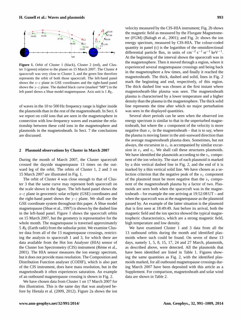
Fig. 1. Orbit of Cluster 1 (black), Cluster 2 (red), and Cluster 3 (green) relative to the planet on 15 March 2007.

The Cluster 4 spacecraft was very close to Cluster 3, and the green line therefore represents the orbit of both

those spacecraft. The left-hand panel shows the x−z plane in GSE coordinates and the right-hand panel shows

the y−z plane. The dashed black curve (marked “MP”) in the left panel shows a Shue model magnetopause.

The distance between two ticks on the axes is 1RE.

In this work, we examine Cluster data from the month of March 2007. During that month the

outbound leg of the Cluster orbit crossed the magnetopause close to the subsolar point on thirteen

occasions. We find plasmoids with larger velocities than the surrounding magnetosheath approach-95

ing the magnetopause from the direction of the bow shock on about half of those days. Section 2

describes how the complete data set is searched for plasmoids, and these are identified and tabulated.

The spatial extent of the plasmoids is determined in section 3. In section 4 we examine in more detail

two plasmoids that were detected by Cluster 1 on 15 March 2007. One of these was observed at the

magnetopause and the other in the magnetosheath. We report on the properties of waves inside these100

plasmoids, and on cold ions that were seen in the magnetosphere immediately after the plasmoid

was detected by the spacecraft. In section 5 it is shown that the energy density of waves in the 10Hz

to 500Hz frequency range is higher inside the plasmoids than in the rest of the magnetosheath. In

section 6 we report on cold ions that are seen in the magnetosphere in connection with low frequency

waves and examine the relationship between these cold ions in the magnetosphere and plasmoids in105

the magnetosheath. In section 7 the conclusions are discussed.

2 Plasmoid observations by Cluster in March 2007

During the month of March 2007, the Cluster spacecraft crossed the dayside magnetopause 13 times

on the outward leg of the orbit. The orbits of Cluster 1, 2, and 3 on 15 March 2007 are illustrated

in Fig. 1. The orbit of Cluster 4 was close enough to that of Cluster 3 that the same curve may110

represent both spacecraft on the scale shown in the figure. The left-hand panel shows the x−z plane

in geocentric solar ecliptic (GSE) coordinates and the right-hand panel shows the y−z plane. We

shall use the GSE coordinate system throughout this paper. A Shue model magnetopause (Shue et al.,

1997) is shown by the dashed line in the left-hand panel. Fig. 1 shows the spacecraft orbits on 15

March 2007, but the geometry is representative for the whole month. The magnetopause is traversed115

approximately 5RE (earth radii) from the subsolar point. We examine Cluster data from all of the

13 magnetopause crossings, restricting the analysis to spacecraft 1 and 3, for which there is data

4

Figure 1. Orbit of Cluster 1 (black), Cluster 2 (red), and Clus-ter 3 (green) relative to the planet on 15 March 2007. The Cluster 4spacecraft was very close to Cluster 3, and the green line thereforerepresents the orbit of both those spacecraft. The left-hand panelshows thex–z plane in GSE coordinates and the right-hand panelshows they–z plane. The dashed black curve (marked “MP”) in theleft panel shows a Shue model magnetopause. Axis unit is 1RE.

of waves in the 10 to 500 Hz frequency range is higher insidethe plasmoids than in the rest of the magnetosheath. In Sect.6we report on cold ions that are seen in the magnetosphere inconnection with low-frequency waves and examine the rela-tionship between these cold ions in the magnetosphere andplasmoids in the magnetosheath. In Sect.7 the conclusionsare discussed.

2 Plasmoid observations by Cluster in March 2007

During the month of March 2007, the Cluster spacecraftcrossed the dayside magnetopause 13 times on the out-ward leg of the orbit. The orbits of Cluster 1, 2 and 3 on15 March 2007 are illustrated in Fig.1.

The orbit of Cluster 4 was close enough to that of Clus-ter 3 that the same curve may represent both spacecraft onthe scale shown in the figure. The left-hand panel shows thex–z plane in geocentric solar ecliptic (GSE) coordinates andthe right-hand panel shows they–z plane. We shall use theGSE coordinate system throughout this paper. A Shue modelmagnetopause (Shue et al., 1997) is shown by the dashed linein the left-hand panel. Figure1 shows the spacecraft orbitson 15 March 2007, but the geometry is representative for thewhole month. The magnetopause is traversed approximately5 RE (Earth radii) from the subsolar point. We examine Clus-ter data from all of the 13 magnetopause crossings, restrict-ing the analysis to spacecraft 1 and 3, for which there aredata available from the Hot Ion Analyser (HIA) sensor ofthe Cluster Ion Spectrometry (CIS) instrument (Rème et al.,2001). The HIA sensor measures the ion energy spectrum,but it does not provide mass resolution. The Composition andDistribution Function analyser (CODIF), which is also partof the CIS instrument, does have mass resolution, but in themagnetosheath it often experiences saturation. An exampleof an outbound magnetopause crossing is shown in Fig.2.

We have chosen data from Cluster 1 on 17 March 2007 forthis illustration. This is the same day that was analysed be-fore byHietala et al.(2009, 2012). Figure2a shows the ion

velocity measured by the CIS-HIA instrument; Fig.2b showsthe magnetic field as measured by the Fluxgate Magnetome-ter (FGM) (Balogh et al., 2001); and Fig.2c shows the ionenergy spectrum, measured by CIS-HIA. The colour-codedquantity in panel (c) is the logarithm of the omnidirectionaldifferential particle flux, in units of cm−2 s−1 sr−1 keV−1.At the beginning of the interval shown the spacecraft was inthe magnetosphere. Then it moved through a region, where itexperienced several magnetopause crossings and being backin the magnetosphere a few times, and finally it reached themagnetosheath. The thick, dashed and solid, lines in Fig.2mark the beginning and end, respectively, of this region.The thick dashed line was chosen at the first instant wheremagnetosheath-like plasma was seen. The magnetosheathplasma is characterised by a lower temperature and a higherdensity than the plasma in the magnetosphere. The thick solidline represents the time after which no major perturbationwas seen in the displayed quantities.

Several short periods can be seen when the observed ionenergy spectrum is similar to that in the unperturbed magne-tosheath, but where thex component of the velocity is morenegative thanvx in the magnetosheath – that is to say, wherethe plasma is moving faster in the anti-sunward direction thanthe average magnetosheath plasma does. Sometimes, but notalways, the excursion invx is accompanied by similar excur-sion in vy andvz. We shall call these structures plasmoids.We have identified the plasmoids according to thevx compo-nent of the ion velocity. The start of each plasmoid is markedby a thin vertical dashed line in Fig.2, and the end of it ismarked by a thin vertical solid line. We have chosen as a se-lection criterion that the negative peak of thevx componentof the plasmoid must be more negative than thevx compo-nent of the magnetosheath plasma by a factor of two. Plas-moids are seen both when the spacecraft was in the magne-tosheath – for example the one arriving at 19:52:08 UT – andwhen the spacecraft was at the magnetopause as the plasmoidpassed by. An example of the latter situation is the plasmoidthat is first seen at 18:49:49. Just before its arrival, both themagnetic field and the ion spectra showed the typical magne-tospheric characteristics, which are a strong magnetic field,high temperature and low density.

We have examined Cluster 1 and 3 data from all the13 outbound orbits during the month and identified plas-moids where such could be found. On seven of these 13days, namely 1, 5, 8, 15, 17, 24 and 27 March, plasmoids,as described above, were detected. All the plasmoids thathave been identified are listed in Table1. Figures show-ing the same quantities as Fig.2, with the identified plas-moids marked, for all outbound magnetopause crossings dur-ing March 2007 have been deposited with this article as aSupplement. For comparison, magnetosheath and solar winddata are shown in Table2.

www.ann-geophys.net/32/991/2014/ Ann. Geophys., 32, 991–1009, 2014


Figure 2. Illustration of plasmoid identification in Cluster 1 data from 17 March 2007.(a) Ion velocity measured by the CIS-HIA instrument.(b) Magnetic flux density measured by the FGM instrument.(c) Omnidirectional ion energy spectrum measured by the CIS-HIA instrument.The colour-coded quantity is the logarithm of the omnidirectional differential particle flux, in units of cm−2 s−1 sr−1 keV−1. The start ofeach plasmoid is marked by a thin vertical dashed line, and the end of it is marked by a thin vertical solid line. The thick, dashed and solid,lines mark the beginning and end of the region where plasmoids are seen. The velocity and magnetic field are shown in GSE coordinates.

The solar wind speed was measured by the Wind space-craft, and the tabulated values are the mean values in the in-terval when the Cluster spacecraft passed through the transi-tion region where plasmoids were observed, as shown by thethick vertical lines in Fig.2. A delay of1x(t)/vx(t) resultingfrom the Wind spacecraft being located upstream was takeninto account. Here1x(t) denotes the difference between thex coordinates of the Wind and Cluster 1 spacecraft andvx(t)

is thex component of the solar wind velocity measured byWind. The magnetosheath values were measured by Clus-ter 1 and 3 as indicated, and are mean values of the first 10minutes each spacecraft spent in the plasmoid-free magne-tosheath.

3 Upper limits of the plasmoid size

In this paper we attribute certain properties to plasmoids. Itis therefore important to show that the observed structurescan be classified as such. In addition to the plasma proper-ties discussed in the previous section, one should also requirethat their size is small enough in comparison with the crosssection of the magnetosphere and the thickness of the mag-netosheath. If they are larger than the cross section of themagnetosphere, the diameter of which is about 10RE at theregion of the dayside where these observations were made,they should rather be seen as pulses of dynamic pressure inthe solar wind. If they are much larger than the thicknessof the magnetosheath, which is about 5RE, they would be

better described as continuous plasma streams. In this sec-tion we examine the spatial extent of the plasmoids by seek-ing upper limits to the plasmoid size in the direction of theflow and in the direction perpendicular to it. The values weobtain overestimate the plasmoid dimensions, enabling us toestablish that the majority of the observed structures are in-deed well described by the term plasmoid.

The duration of each plasmoid observation can be used toestimate their size in the direction of the flow. For this pur-pose the productT · max(|v|) of the duration and maximumspeed values in Table1 can be used as an upper limit. For the64 plasmoids in the table, this limit is in a range from 0.5 REto 20RE with a median value of 4.9 RE, which means that ina majority of cases, the estimated upper limit of the plasmoidsize is less than 5RE. It is seen in Fig.3b that there can belarge fluctuations invx within a plasmoid. It is not obviouswhether one should consider two negativevx peaks that fol-low immediately after each other as two separate plasmoidsor as being part of a single plasmoid that shows large fluc-tuations. In such cases, we have counted them as belongingto the same plasmoid. This may affect the size estimate. Thepreference for larger plasmoids contributes to increasing theestimated size.

To form an estimate in the direction perpendicular tothe flow we rely on simultaneous measurements by Clus-ter 1 and 3. Figure3 shows data taken by these two space-craft around 19:00 on 17 March 2007. Panels (a) and (b)show the GSE components of the ion velocity for Clus-ter 1 and 3 respectively. Panel (c) shows the magnetic field



Table 1. Plasmoids identified in the data from March 2007. The columns show the first time that the plasmoid was observed; its durationT ; the spacecraft that observed it; the maximum value of the plasma speed, max(|v|), within the plasmoid; the most negativevx value; themaximum density max(n); and the mean energy density of the magnetic〈PBB/µ0〉 and electric〈ε0PEE〉 fluctuations in the frequency range10 Hz≤ f ≤ 500 Hz, measured by the STAFF instrument.

Start T s/c max(|v|) min(vx) max(n) 〈PBB/µ0〉〈ε0PEE〉

(s) (km s−1) (km s−1) (m−3) (J m−3) (J m−3)

2007-03-01 02:55:56 41 C3 334 −334 2.0× 107 1.9× 10−14 3.5× 10−19

2007-03-01 02:56:09 100 C1 359 −354 2.3× 107 1.8× 10−14 9.1× 10−19

2007-03-01 03:10:00 309 C3 335 −289 2.3× 107 3.7× 10−15 1.4× 10−19

2007-03-01 03:10:49 174 C1 410 −386 2.1× 107 7.3× 10−15 1.7× 10−19

2007-03-01 03:58:49 203 C3 403 −369 3.5× 107 1.6× 10−14 1.3× 10−18

2007-03-01 04:01:04 137 C1 394 −380 1.8× 107 1.8× 10−14 1.3× 10−18

2007-03-01 04:09:59 78 C3 470 −440 2.1× 107 3.6× 10−14 2.5× 10−18

2007-03-01 04:11:18 29 C1 434 −402 2.3× 107 1.3× 10−13 3.8× 10−18

2007-03-01 04:22:58 76 C3 370 −327 1.4× 107 3.2× 10−15 1.2× 10−19

2007-03-05 18:53:21 93 C1 435 −318 1.8× 107 3.8× 10−13 3.0× 10−17

2007-03-05 18:53:30 45 C3 247 −158 2.4× 107 4.2× 10−14 4.2× 10−17

2007-03-05 18:55:14 313 C1 349 −238 2.7× 107 2.1× 10−13 3.3× 10−17

2007-03-05 18:56:23 144 C3 368 −208 3.3× 107 1.3× 10−13 4.7× 10−17

2007-03-05 18:59:04 79 C3 348 −200 3.4× 107 3.4× 10−13 3.2× 10−17

2007-03-05 19:02:02 21 C3 277 −145 3.0× 107 3.9× 10−13 3.7× 10−17

2007-03-05 19:02:14 25 C1 253 −176 2.4× 107 2.3× 10−13 1.1× 10−17

2007-03-05 19:07:57 282 C1 363 −247 2.2× 107 9.2× 10−14 3.7× 10−17

2007-03-05 19:12:02 24 C3 446 −298 1.6× 106 2.1× 10−16 1.0× 10−17

2007-03-05 19:15:16 91 C3 418 −231 1.9× 107 3.0× 10−13 7.4× 10−17

2007-03-05 19:16:10 67 C1 306 −183 2.4× 107 1.1× 10−13 4.1× 10−17

2007-03-08 07:44:51 148 C3 106 −93 6.6× 106 4.8× 10−16 1.5× 10−19

2007-03-08 09:03:10 128 C3 196 −130 9.0× 106 2.1× 10−15 3.3× 10−20

2007-03-15 08:00:39 159 C1 404 −394 2.1× 107 3.0× 10−13 7.0× 10−17

2007-03-15 08:09:01 58 C1 521 −468 1.2× 107 3.9× 10−13 1.7× 10−17

2007-03-15 09:32:57 37 C1 368 −336 1.1× 107 1.3× 10−13 1.7× 10−17

2007-03-15 09:53:58 21 C1 514 −504 1.3× 107 2.1× 10−13 7.8× 10−18

2007-03-15 09:55:09 104 C1 587 −523 2.1× 107 4.7× 10−13 2.9× 10−17

2007-03-15 10:14:59 71 C1 526 −514 1.3× 107 1.1× 10−12 1.5× 10−16

2007-03-15 10:21:05 29 C1 444 −441 1.8× 107 8.4× 10−13 9.2× 10−17

2007-03-15 10:23:26 20 C1 542 −503 8.2× 106 1.1× 10−12 1.0× 10−16

2007-03-17 17:24:58 50 C3 425 −306 2.0× 107 1.0× 10−14 7.5× 10−18

2007-03-17 17:25:04 74 C1 424 −206 2.5× 107 1.2× 10−14 5.4× 10−18

2007-03-17 17:31:23 272 C3 383 −321 2.3× 107 5.7× 10−15 3.9× 10−19

2007-03-17 17:32:15 166 C1 394 −199 2.2× 107 5.3× 10−15 4.6× 10−19

2007-03-17 17:56:19 74 C3 336 −234 1.8× 107 2.7× 10−15 5.8× 10−18

2007-03-17 17:58:24 165 C1 415 −383 1.9× 107 2.9× 10−15 1.9× 10−19

2007-03-17 17:58:39 108 C3 335 −329 1.3× 107 2.7× 10−15 1.3× 10−19

2007-03-17 18:04:02 177 C3 449 −438 3.2× 107 7.4× 10−15 9.4× 10−19

2007-03-17 18:04:12 203 C1 464 −395 2.8× 107 1.1× 10−14 4.8× 10−19

2007-03-17 18:13:24 231 C3 499 −491 2.4× 107 8.9× 10−15 1.7× 10−18

2007-03-17 18:13:36 150 C1 498 −493 1.9× 107 1.3× 10−14 8.9× 10−19

2007-03-17 18:31:31 260 C3 475 −450 1.8× 107 2.3× 10−15 6.6× 10−19

2007-03-17 18:31:52 215 C1 386 −372 2.0× 107 4.5× 10−15 1.2× 10−18

2007-03-17 18:49:49 217 C1 361 −340 1.8× 107 4.7× 10−15 2.0× 10−18

2007-03-17 18:50:32 74 C3 331 −289 1.9× 107 3.7× 10−15 5.4× 10−19

2007-03-17 18:53:46 116 C3 295 −293 2.5× 107 1.1× 10−14 1.8× 10−18

2007-03-17 19:02:47 124 C3 330 −303 1.5× 107 3.5× 10−15 8.5× 10−19

2007-03-17 19:05:57 33 C1 375 −364 1.5× 107 3.4× 10−15 3.9× 10−19

2007-03-17 19:34:54 70 C3 457 −405 1.6× 107 3.0× 10−15 1.5× 10−18

2007-03-17 19:35:53 25 C1 424 −376 1.5× 107 2.2× 10−15 2.7× 10−19

2007-03-17 19:52:08 100 C1 373 −345 1.7× 107 3.1× 10−15 2.1× 10−19

2007-03-17 19:52:32 95 C3 480 −458 1.8× 107 6.0× 10−15 1.7× 10−18

2007-03-17 20:14:39 57 C3 320 −183 1.5× 107 1.6× 10−15 1.5× 10−19

2007-03-24 19:09:55 33 C3 106 −86.4 2.1× 106 1.0× 10−17 3.5× 10−18

2007-03-24 19:35:13 162 C1 392 −212 3.8× 107 4.5× 10−15 2.0× 10−17

2007-03-24 19:37:20 33 C3 299 −130 1.7× 107 5.1× 10−16 2.0× 10−17

2007-03-24 20:01:26 29 C1 173 −151 1.3× 107 2.3× 10−16 4.7× 10−17

2007-03-24 20:04:28 104 C1 214 −171 2.5× 107 1.3× 10−15 4.6× 10−18

2007-03-24 20:07:18 87 C3 244 −160 1.5× 107 3.9× 10−16 1.3× 10−17

2007-03-27 05:07:03 66 C1 479 −195 2.0× 107 7.5× 10−15 9.1× 10−17

2007-03-27 05:57:37 98 C3 190 −179 5.0× 107 10.0× 10−15 1.8× 10−19

2007-03-27 06:00:50 136 C3 200 −189 6.2× 107 1.2× 10−14 1.3× 10−18

2007-03-27 06:07:35 99 C3 203 −179 4.9× 107 1.5× 10−14 6.3× 10−19

2007-03-27 06:13:22 54 C1 197 −190 6.0× 107 1.6× 10−14 1.2× 10−18

2007-03-27 06:15:14 111 C3 286 −262 3.9× 107 1.1× 10−14 1.1× 10−18



Figure 3. Comparison of data from Cluster 1 and 3 on 17 March 2007.(a) Ion velocity components in GSE coordinates for Cluster 1.(b) Ionvelocity for Cluster 3.(c) Magnetic flux density for Cluster 3.(d) Omnidirectional ion energy spectrum. The colour coded quantity is thelogarithm of the omnidirectional differential particle flux, in units of cm−2 s−1 sr−1 keV−1. The start of each plasmoid is marked by avertical dashed line, and the end of it is marked by a vertical solid line. For Cluster 1 these quantities are shown for a longer period in Fig.2

and panel (d) the omnidirectional ion energy spectrum ob-served by Cluster 3. The magnetic field and ion energy spec-trum for Cluster 1 is shown in Fig.2, although on a dif-ferent timescale. The vertical dashed and solid lines markthe beginning and end, respectively, of each identified plas-moid during the period shown. This example has been cho-sen because both spacecraft were in the magnetosheath, asis seen from the magnetic field and ion spectra, and there-fore estimate is not influenced by the response of the mag-netopause to the plasmoid impact. At 19:00 the position ofCluster 1 wasrC1 = (11.6; 1.8; 2.5) RE and that of Clus-ter 3 rC3 = (11.9; 0.55; 1.9) RE, and the resulting space-craft separation wasrC1− rC3 = (−1755; 7999; 4212) km.With this separation, and thevx values in the plasmoids, astructure of large spatial extent in the direction perpendicularto thex axis would first be seen at Cluster 3 and then at Clus-ter 1 after about 5–9 s. It is possible that the first plasmoidseen by Cluster 1 in Fig.3a is the same one that was seen byCluster 3, which then passed through a smaller part of it. It isalso possible that the two spacecraft observed two differentplasmoids. Short of having a large number of spacecraft linedup between Cluster 1 and 3 this is impossible to determine, asplasma properties are likely to vary between different parts ofthe same plasmoid. The two later plasmoids seen by Cluster 3are not seen by Cluster 1, and the last one seen by Cluster 1 isnot seen by Cluster 3. The delay between the last plasmoidsfor each spacecraft in the figure is more than a minute, which

is much more than the 5–9 s that would be expected underthe assumption of a large perpendicular extent.

During the days when data from the CIS-HIA instrumentson both Cluster 1 and Cluster 3 were available 24 plasmoidswere seen by Cluster 1 and 31 by Cluster 3. Of the 24 plas-moids that Cluster 1 observed, 18 overlapped completely orpartially with plasmoids seen by Cluster 3, using the plas-moid durations in Table1. If we allow for a 30 s delay be-tween the spacecraft, a time confidently longer than the 5–9 s cited above, this number increases to 19. Taking care notto underestimate the plasmoid size, we count overlappingobservations by the two spacecraft as both of these havingobserved one and the same plasmoid. This means that weprobably overestimate the plasmoid size, as it is likely that insome of the cases the two spacecraft each observed differentindividual plasmoids.

Given that the spacecraft separation in a plane perpendic-ular to thex axis wasS = 1.4 RE, one may estimate the per-pendicular extent of the plasmoids. This was done by assum-ing plasmoids of circular cross section in the plane perpen-dicular to thex axis that are positioned at random in thatplane. The method is illustrated in Fig.4. The plasmoid isshown by the large black circle with radiusR. If Cluster 1 isin the green area, Cluster 3 is also inside the plasmoid, and ifCluster 1 is in the white crescent-shaped region, Cluster 3 isoutside of the plasmoid. The probabilitypA that both space-craft see the plasmoid, given that Cluster 1 does, is the ratio



C1

C1

C3

C3

R

S

S

S

Fig. 4. Illustration of the method by which the perpendicular plasmoid extent is estimated. The plasmoid is

shown by the large black circle with radius R. If Cluster 1 is in the green area, Cluster 3 is also inside the

plasmoid. If Cluster 1 is in the white crescent-shaped area, Cluster 3 is outside the plasmoid. The spacecraft

positions, marked “×”, show examples of the two situations.

about R=10RE. The plasmoid description is thus more suitable than that of a solar wind dynamic

pressure pulse. As we are overestimating the size, the majority of the plasmoids are smaller than

7RE. The median value of the plasmoid extent in the direction of the plasma flow is R= 4.9RE,

which is approximately the same as the thickness of the magnetosheath. This means that at least

half of the plasmoids should at some instant in time be detached from both the bow shock and the240

magnetopause. To make the opposite interpretation, namely that of a continuous plasma stream, one

should require a plasmoid that is much larger than the magnetosheath thickness.

In the direction along the plasma flow, Nemecek et al. (1998) found that the dimensions of the

plasmoids they observed were “in the range of units of RE”; Plaschke et al. (2013b) estimated the

median extent to 4000 km, and the dimensions found by Archer et al. (2012) were approximately245

1RE. Considering that we overestimate the parallel dimension by using the maximum plasma speed

inside the plasmoid instead of integrating the velocity, our estimate is not in disagreement with the

previous authors.

In the direction perpendicular to the flow, Archer et al. (2012) estimated the spatial dimensions

from the spacecraft separation without considering what fraction of the plasmoids were observed by250

both spacecraft. Their estimate of 0.2-0.5RE is therefore likely an underestimate. Our value of a

3.6RE radius is an overestimate, and the true value should be in between. However, there is a wide

12

Figure 4. Illustration of the method by which the perpendicularplasmoid extent is estimated. The plasmoid is shown by the largeblack circle with radiusR. If Cluster 1 is in the green area, Clus-ter 3 is also inside the plasmoid. If Cluster 1 is in the white crescent-shaped area, Cluster 3 is outside the plasmoid. The spacecraft posi-tions, marked “×”, show examples of the two situations.

of the green area to the total area of the circle:

pA =2R2arccos

(S

2R

)−

S2

√4R2 − S2

πR2. (1)

If 18 of the 24 plasmoids observed at Cluster 1 also wereobserved by the other spacecraft, we havepA = 0.75, as-suming that we observed the most likely outcome. SolvingEq. (1) numerically withpA = 0.75 andS = 1.4 RE, we ob-tain R = 3.6 RE, which we take as an order of magnitudeestimate of the perpendicular extent. With the same num-bers reported above one could use the 31 plasmoids seenby Cluster 3 and the 18 simultaneous observations to obtainpA = 18/31≈ 0.58, which corresponds toR = 2.1 RE. Aswe are looking for an upper limit we shall use the highervalue ofR = 3.6 RE.

The conclusion of this section is that the plasma entitiesconsidered can be described as plasmoids. The estimatedplasmoid radius ofR = 3.6 RE corresponds to a diameter of7.2 RE, which is below the diameter of the magnetopause atthe part of the dayside where the observations were made,which is aboutR = 10RE. The plasmoid description is thusmore suitable than that of a solar wind dynamic pressurepulse. As we are overestimating the size, the majority ofthe plasmoids are smaller than 7RE. The median value ofthe plasmoid extent in the direction of the plasma flow isR = 4.9 RE, which is approximately the same as the thick-ness of the magnetosheath. This means that at least half ofthe plasmoids should at some instant in time be detachedfrom both the bow shock and the magnetopause. To make theopposite interpretation, namely that of a continuous plasmastream, one should require a plasmoid that is much largerthan the magnetosheath thickness.

In the direction along the plasma flow,Nemecek et al.(1998) found that the dimensions of the plasmoids they ob-served were “in the range of units ofRE”; Plaschke et al.(2013b) estimated the median extent to 4000 km, and the di-mensions found byArcher et al.(2012) were approximately1 RE. Considering that we overestimate the parallel dimen-sion by using the maximum plasma speed inside the plas-moid instead of integrating the velocity, our estimate is notin disagreement with the previous authors.

In the direction perpendicular to the flow,Archer et al.(2012) estimated the spatial dimensions from the spacecraftseparation without considering what fraction of the plas-moids were observed by both spacecraft. Their estimate of0.2–0.5RE is therefore likely an underestimate. Our value ofa 3.6 RE radius is an overestimate, and the true value shouldbe in between. However, there is a wide spread in the distri-bution of sizes, as was shown byKarlsson et al.(2012), whoobserved a size range spanning from 0.1 RE to 10RE.

4 Details of two plasmoids

We examine two plasmoids that were observed at themagnetopause and in the magnetosheath respectively on15 March 2007. On this date CIS-HIA data were not avail-able for Cluster 3. Therefore, the study of these particu-lar plasmoids is limited to a single spacecraft. Figure5shows a summary of the data obtained by Wind and Clus-ter 1 on 15 March 2007. The Wind spacecraft was locatedat (x,y,z) = (199,−42,−18) RE, which means that it takesthe plasma about 31 minutes to move from the Wind space-craft to the position of the Cluster spacecraft. This delay hasbeen taken into account in Fig.5, showing all data on theCluster 1 time base, which means that the time plotted inpanels (a) and (b) istC1 = tW +1x(tW)/vx(tW), wheretW isthe wind time base,1x(tW) denotes the difference betweenthe x coordinates of the Wind and Cluster 1 spacecraft andvx(tW) is thex component of the solar wind velocity mea-sured by Wind. Panel (a) shows the solar wind magnetic fieldand panel (b) shows the solar wind dynamic pressure, bothmeasured by Wind. Panel (c) shows the magnetic field mea-sured by the FGM instrument on Cluster 1. Panel (d) showsthe bulk velocity of the ions and panel (e) the ion density,both measured by CIS-HIA. Panel (f) shows the electron en-ergy spectrum measured by the Plasma Electron and CurrentExperiment (PEACE) instrument (Johnstone et al., 1997) forenergies above 1 keV. The colour-coded quantity is the loga-rithm of the omnidirectional differential particle flux, in unitsof cm−2 s−1 sr−1 keV−1. Finally, panel (g) of Fig.5 showsthe ion energy spectrum measured by CIS-HIA. Like in thecase of the electron spectrum, the colour-coded quantity isthe logarithm of the omnidirectional differential particle flux,in units of cm−2 s−1 sr−1 keV−1. The magnitude of the solarwind magnetic field showed only small variations, althoughits direction varied during the period in question. Also the



Table 2. Magnetosheath and solar wind data. The solar wind speed and magnetic field were measured by the Wind spacecraft. The mag-netosheath values are mean values of the first 10 min Cluster 1 and 3, respectively, spent in the magnetosheath after the last plasmoid wasseen.

Date |vSW| |vMS| BMS

C1 C3 C1 C3(km s−1) (km s−1) (km s−1) (nT) (nT)

2007-03-01 610 180 168 (−2.4, 12, 8.5) (−3.4, 13,−7.8)2007-03-03 358 74 58 (−11, 15, 26) (−7.6, 16, 26)2007-03-05 393 116 101 (12,−13,−21) (13,−16,−26)2007-03-08 475 – 67 (1.5,−13, 3.6) (0.91,−13, 3.6)2007-03-10 343 125 100 (8.5,−25,−6.0) (7.3,−28,−7.2)2007-03-12 601 191 154 (−4.6, 32,−16) (−2.7, 33,−17)2007-03-15 637 180 – (−0.72, 10,−6.3) (−0.5, 10,−5.8)2007-03-17 535 148 102 (−2.3, 5.6, 9.0) (−0.89, 9.6, 7)2007-03-20 344 54 41 (−0.58, 17,−2.9) (1.1, 17,−3.2)2007-03-22 269 64 55 (3.3,−23,−7.7) (1.8,−25,−7.5)2007-03-24 350 113 73 (−19,−24, 54) (−18,−17, 61)2007-03-27 447 93 76 (−3.5, 31, 4.9) (−0.37, 30, 3.8)2007-03-29 397 86 66 (−0.066, 25,−3.1) (1.5, 21,−2.3)

solar wind dynamic pressure was relatively constant. TheDst and Kp indices showed a moderate geomagnetic activity.Throughout 15 March Dst was above−20 nT, and its meanvalue between midnight and noon was−11.75 nT. The Kpindex was 2+ from 03:00 to 06:00; 3− between 06:00 and09:00; and 2 from 09:00 to 12:00.

At the start of the interval shown in Fig.5 the space-craft is inside the magnetosphere, and as it moves outward itreaches the magnetopause at 08:00:39 UT. This is when wehave identified the first plasmoid. After the passage of theplasmoid, the spacecraft found itself in the magnetosphereagain and stayed there until the arrival of the next plasmoidat 08:09:01. In the period between the second plasmoid ob-servation and 08:30 a few magnetopause crossings were seenthat did not coincide with plasmoid detections. After thattime the spacecraft was in the magnetosheath, away from themagnetopause. There, several plasmoids were observed untilabout 10:30, and after this time no plasmoids were seen.

Apart from the defining feature of the plasmoids, that is tosay, that thevx component of the velocity (Fig.5d) reachesa large negative value, we see that the density increases fromthe low levels of the magnetosphere to a level of the or-der of the magnetosheath density for those plasmoids thatare observed at the magnetopause. For those that were ob-served in the magnetosheath, farther away from the magne-topause, the density is already at magnetosheath levels and,while a relative increase can be seen at some plasmoids itis less conspicuous. Similarly, a large and rapid change wasseen in the magnetic field only for plasmoids observed at themagnetopause. The high-energy electron spectrum (Fig.5f)is magnetosheath-like inside the plasmoids, which indicatesthat these were not on the closed field lines of the mag-netosphere. The ion spectrum (Fig.5g), on the other hand,

shows that high-energy ions, from 10 keV and upward, werepresent occasionally during the period when plasmoids ap-peared. This is seen in Fig.5g when the observed flux above10 keV is similar to that of the magnetosphere, for exampleat 09:04, 09:37 and 10:19, but also at many other times, andabout two orders of magnitude higher than that of the mag-netosheath after 10:30.

The first and the next to last plasmoids that are shown inFig. 5 (marked by downward pointing black triangles aboveFig. 5c) are enlarged in Figs.6 and7.

The plasmoid that was observed at the magnetopause at08:00:39 on 15 March 2007 by Cluster 1 is shown in Fig.6.The plasmoid speed was larger than the average magne-tosheath speed by more than a factor of two. The velocitywas directed mostly in the negativex direction. The veloc-ity direction is illustrated by the red arrows in Fig.8 whichshows position of the Cluster 1 spacecraft (marked by blackcircles) at 08:00 and 10:21 on 15 March 2007. The posi-tions of the three other spacecraft at 08:00 are marked withplus signs. The left-hand panel shows thex–z plane and theright-hand panel shows they–z plane. A Shue model mag-netopause (Shue et al., 1997) is shown by the dashed line inthe left-hand panel. The solar wind parameters used as in-put to the Shue model were mean values of measurementsby the Wind spacecraft over the period from 08:00 to 08:10in Fig. 5. The magnetic field direction on the inside of themagnetopause is shown by the blue arrows. The velocity thatis shown by the arrow in Fig.8 is the velocity at the time ofthe negativevx peak in Fig.6b. The magnetic field directionis an average ofB observed by FGM between 60 and 30 sbefore the arrival of the plasmoid, and it thus represents thedirection of the magnetic field inside the magnetosphere.



Figure 5. Data obtained by the Wind and Cluster 1 spacecraft on 15 March 2007.(a) Solar wind magnetic fieldBx (blue),By (green),Bz

(red), and|B| (black); and(b) solar wind dynamic pressure, both measured by the Wind spacecraft. Panels(c–g)show data from Cluster 1.(c) Magnetic fieldBx (blue), By (green), andBz (red); (d) ion velocity vx (blue), vy (green), andvz (red); (e) ion density;(f) electronenergy spectrum above 1 keV, with the colour coded scale showing the logarithm of the omnidirectional differential particle flux in unitsof cm−2 s−1 sr−1 keV−1; and(g) the ion energy spectrum, where the colour scale shows the logarithm of the omnidirectional differentialparticle flux, in units of cm−2 s−1 sr−1 keV−1. The components of the vector quantities in panels(a), (c), and (d) are shown in GSEcoordinates. The vertical lines mark the plasmoids that have been identified in Table1. The first and the next to last plasmoids (marked bydownward pointing black triangles above panelc) are discussed in the text, and they are shown on a larger scale in Figs.6 and7.

The magnetic field in the plasmoid is weaker than thatof the magnetosphere and its direction is variable as isseen in Fig.6a. At the time of the most negativevx therewas a large component of the plasmoid velocity perpendic-ular to the magnetic field in the magnetosphere, and, as-suming that the field is at least approximately in the planeof the magnetopause, the velocity was also largely per-pendicular to the magnetopause. This is confirmed by ananalysis of the magnetopause crossing times, determinedfrom the magnetic field data of the four spacecraft (C1crossed the magnetopause at 08:00:53.3; C2 at 08:00:41.6;C3 at 08:00:28.4; and C4 at 08:00:35.6), which gives a

magnetopause moving in the direction of its normal at a ve-locity v = (−107; 11.4; −15.3) km s−1. The magnetopausenormal is dominated by itsx component.

Towards the end of the plasmoid observationvx changessign and becomes positive. This indicates that the plasmoidmade an indentation on the magnetopause and then bouncedback, in the same way as in the observation byShue et al.(2009). This type of magnetopause motion can be comparedto that which is caused by a surface wave as was observedby Plaschke et al.(2013a). With three of the THEMIS space-craft, one at the magnetopause and one on either side of it,those authors were able to measure the velocity field of a



Figure 6. Data obtained by Cluster 1 on 15 March 2007. On thehorizontal axis, timet = 0 corresponds to 08:00:39 UT.(a) Mag-netic flux density in GSE coordinates;(b) ion bulk velocity inGSE coordinates;(c) ion density;(d) omnidirectional ion energyspectrum;(e) the x component ofB measured by STAFF in the0.6 Hz≤ f ≤ 180 Hz frequency range;(f) power spectral densityof |B|; (g) power spectral density of|E|; (h) propagation angle, i.e.the angle betweenk andB; (i) ellipticity; (j) degree of polarisation.The vertical dashed lines mark the beginning and end of the plas-moid identified in Table1. The blue curves on panels(f–j) show0.1fce (upper curve) andflh (lower curve).

Figure 7. Data obtained by Cluster 1 on 15 March 2007. On thehorizontal axis, timet = 0 corresponds to 10:21:05 UT.(a) Mag-netic flux density in GSE coordinates;(b) ion bulk velocity inGSE coordinates;(c) ion density;(d) omnidirectional ion energyspectrum;(e) the x component ofB measured by STAFF in the0.6 Hz≤ f ≤ 180 Hz frequency range;(f) power spectral densityof |B|; (g) power spectral density of|E|; (h) propagation angle, i.e.the angle betweenk andB; (i) ellipticity; (j) degree of polarisation.The vertical dashed lines mark the beginning and end of the plas-moid identified in Table1. The blue curves on panels(f–j) show0.1fce (upper curve) andflh (lower curve).



B

x

C1 10:21v

MP

C1 08:00

C2

C3,4

Bv

z

y

v

B

B

C1 08:00v

C1 10:21

C2

C3,4

z

Figure 8. Position of the Cluster spacecraft relative to the planet on15 March 2007. The Cluster 1 positions are marked “◦” for the times08:00 and 10:21, and the positions of the other three spacecraft at08:00 are marked “+”: red for C2, green for C3, and blue for C4.The blue arrows show the direction of the magnetic field and thered arrows show the plasmoid velocity direction for the plasmoidsencountered by C1 at 08:00 and 10:21. The magnetic field directionshown is the mean value in the period from 60 to 30 s before theplasmoid arrived at the spacecraft. The left-hand panel shows thex–z plane in GSE coordinates and the right-hand panel shows they–z plane. The dashed black curve in the left panel shows a Shuemodel magnetopause.

magnetopause surface wave that passed by the spacecraft.Also there both magnetosheath plasma and magnetosphericplasma were observed, but the magnetosheath plasma movedtangentially along the magnetopause, and the plasma on themagnetospheric side moved back and forth along the magne-topause normal. In our case, the dense magnetosheath plasmamoves along the normal, driving the magnetopause motion atthe point in space where it was detected by the spacecraft.

On the right-hand side of Fig.6d an ion population whichis narrow in energy can be seen outside the plasmoid justafter the spacecraft re-entered the magnetosphere. This is acold ion population of ionospheric origin. Figure9 showsthe electric field measured by the EFW (Electric Field andWaves) instrument (Gustafsson et al., 2001) during the periodwhen these cold ions were observed. The electric field wasoriented in they direction and peaked atEy = 19 mV m−1,which combined with the magnetic field at the time, shownin Fig. 6a, yields anE × B/B2 drift velocity with both thex andz components near 200 km s−1. This is consistent withthe measured ion velocity shown in Fig.6b. Thus, the mag-netospheric plasma inside the magnetopause is set in motionby the plasmoid impact, and individual particles in the nearmagnetopause magnetosphere experience this as anE × B

drift. In Fig. 5g, which shows the ion spectrum on a longertimescale, the cold plasma can be seen to slow down and thenspeed up again just before the arrival of the next plasmoid at08:09:01.

In Fig. 7 a plasmoid that was detected by Cluster 1 at10:21:05 UT on 15 March 2007 is shown. It is seen in Fig.7aand d that the magnetic field and ion energy spectrum bothbefore and after the plasmoid were typical of the magne-tosheath. Thus this plasmoid was in the magnetosheath, andnot interacting with the magnetopause at the time of obser-vation. The peak negativevx value was close to that of theother plasmoid in Fig.6. The direction of the velocity, at the

140 160 180 200 220 240-5

0

5

10

15

20

t [s]

Ex,

y,z

[mV

/m]

Fig. 9. Electric field measured by the EFW instrument on the Cluster 1 spacecraft after the first plasmoid

observation on 15 March. The time scale is the same as that in Fig. 6. The dashed line at t=159s marks the

end of the plasmoid.

is seen in Figs. 7a and 7d that the magnetic field and ion energy spectrum both before and after the

plasmoid were typical of the magnetosheath. Thus this plasmoid was in the magnetosheath, and not350

interacting with the magnetopause at the time of observation. The peak negative vx value was close

to that of the other plasmoid in Fig. 6. The direction of the velocity, at the time of the peak negative

vx, is illustrated in Fig. 8, and it is in the same direction as for the other plasmoid. The magnetic

field direction that is shown in Fig. 8 is again an average of B observed by FGM between 60 and

30 seconds before the arrival of the plasmoid, and in this case this means that it is a magnetosheath355

field that is shown. The density in the plasmoid is somewhat higher than that of the surrounding

magnetosheath, and the magnetic field exhibits fluctuations.

Figs. 6e and 7e show the oscillating x component of the magnetic field Bx in the 0.6Hz≤ f ≤180Hz frequency range that was measured by the STAFF (Spatio Temporal Analysis of Field Fluc-

tuations) instrument (Cornilleau-Wehrlin et al., 1997). Panels (f-j) of Figs. 6 and 7 show wave360

propagation parameters in the 10Hz≤ f ≤ 180Hz frequency range that were calculated from the

STAFF data using the singular value decomposition method as described by Santolık et al. (2003).

Spectral powers of E and B were obtained using Morlet wavelet analysis. In these two figures, pan-

els (f) show the power spectral density of the magnetic field, PBB , with all three components added

together. Panels (g) show the sum of the power spectral density, PEE , for the two measured electric365

field components. Panels (h) show the propagation angle θ=π/2−|π/2−arccos(k ·B/(|k||B|))|,which means that θ=0 corresponds to k being parallel or anti-parallel to B and θ= π/2 to it be-

ing perpendicular. Panels (i) show the ellipticity, which is defined as the ratio of the minor to the

major axes of the ellipse described by the component of the wave magnetic field, perpendicular to

the wave vector. For waves that are right-hand polarised with respect to B the ellipticity is posi-370

tive. The (j) panels show the degree of polarisation, which represents the ratio between the polarised

part of the wave intensity and the total wave intensity. The degree of polarisation is one for purely

polarised waves and zero for completely unpolarised waves. The blue curves on panels (f-j) show

one tenth of the electron cyclotron frequency, 0.1fce, (upper curve) and the lower hybrid frequency

19

Figure 9. Electric field measured by the EFW instrument onthe Cluster 1 spacecraft after the first plasmoid observation on15 March. The timescale is the same as that in Fig.6. The dashedline att = 159 s marks the end of the plasmoid.

time of the peak negativevx , is illustrated in Fig.8, and itis in the same direction as for the other plasmoid. The mag-netic field direction that is shown in Fig.8 is again an av-erage ofB observed by FGM between 60 and 30 s beforethe arrival of the plasmoid, and in this case this means thatit is a magnetosheath field that is shown. The density in theplasmoid is somewhat higher than that of the surroundingmagnetosheath, and the magnetic field exhibits fluctuations.

Figures6e and7e show the oscillatingx component ofthe magnetic fieldBx in the 0.6 Hz≤ f ≤ 180 Hz frequencyrange that was measured by the STAFF (Spatio Tempo-ral Analysis of Field Fluctuations) instrument (Cornilleau-Wehrlin et al., 1997). Panels (f–j) of Figs.6 and 7 showwave propagation parameters in the 10 Hz≤ f ≤ 180 Hzfrequency range that were calculated from the STAFF datausing the singular value decomposition method as describedby Santolík et al.(2003). Spectral powers ofE and B

were obtained using Morlet wavelet analysis. In these twofigures, panels (f) show the power spectral density of themagnetic field,PBB, with all three components added to-gether. Panel (g) shows the sum of the power spectraldensity, PEE, for the two measured electric field compo-nents. Panel (h) shows the propagation angleθ = π/2−

|π/2−arccos(k · B/(|k||B|)) |, which means thatθ = 0 cor-responds tok being parallel or anti-parallel toB and θ =

π/2 to it being perpendicular. Panels (i) show the elliptic-ity, which is defined as the ratio of the minor to the majoraxes of the ellipse described by the component of the wavemagnetic field, perpendicular to the wave vector. For wavesthat are right-hand polarised with respect toB the elliptic-ity is positive. The (j) panels show the degree of polarisa-tion, which represents the ratio between the polarised partof the wave intensity and the total wave intensity. The de-gree of polarisation is one for purely polarised waves andzero for completely unpolarised waves. The blue curves onpanels (f–j) show one tenth of the electron cyclotron fre-quency, 0.1fce, (upper curve) and the lower hybrid frequency

flh = fpi/√

1+ f 2pe/f

2ce (lower curve), wherefpi is the ion



plasma frequency andfpe the electron plasma frequency. Theelectron cyclotron frequency is computed from FGM dataand the plasma frequencies from CIS-HIA data. The quan-tities in panels (h) and (i) are shown only for times and fre-quencies where the degree of polarisation is 0.6 or greater,since these quantities become unreliable for lower degrees ofpolarisation.

A magnetic field signal was measured inside the plasmoidthat arrived at 08:00:39 UT as is seen in Fig.6e. The compo-nentBx is the one component that is shown. However, theother two components both show a similar pattern. In thecase of Fig.6, the spacecraft was inside the magnetosphereboth before and after the encounter with the plasmoid, andthere the amplitude was much lower. This is seen also in thepower spectral density of the magnetic field, which is shownin Fig. 6f and in that of the electric field in Fig.6g. Twodifferent signatures can be distinguished in the power spec-tral density diagram. First, there are fluctuations around thelower hybrid frequency that can be seen in both the electricand magnetic fields. These are present throughout the dura-tion of the plasmoid. Where the degree of polarisation is highenough that anything can be said about it,θ ≈ π/2 in this fre-quency range, as seen in the lower part of Fig.6h, meaningthat these are waves propagating mostly perpendicular toB.Secondly, there are short bursts of wave energy around andabove 0.1fce. While present in both the electric and mag-netic fields, they are more easily distinguished in the mag-netic power spectral density in Fig.6f. Examining panels (h–j) for these bursts we see that they have a high degree of po-larisation, an ellipticity close to 1, and a low propagation an-gle. These bursts can therefore be identified as whistler modewaves. In the near-magnetopause magnetosphere – that is tosay, just before and just after the plasmoid observation – suchwhistler mode waves are seen at 0.1fce during a longer pe-riod, but with a lower amplitude, than that of the burst insidethe plasmoid.

Also for the plasmoid that was encountered at 10:21:05 UTthe oscillatory electric and magnetic energies were larger in-side than in the surrounding plasma. This is seen in panels(e–g) of Fig.7. The difference between the power spectraldensities inside the plasmoid and those in its immediate sur-roundings are not as prominent as those of the other plas-moid, which was shown in Fig.6, because the plasmoid ofFig. 7 was surrounded by magnetosheath plasma, which hasa higher background fluctuation level. Examining Fig.7f–j,it is seen that also in this plasmoid there are bursts of whistlermode waves at and above 0.1fce, and low-frequency wavesof mostly perpendicular propagation appear from aroundflhup to about 0.1fce.

5 Wave amplitude statistics

The wave amplitudes observed inside the two plasmoids ex-amined in Sect.4 were higher than in the plasma observed

by the spacecraft just before and just after the plasmoidencounter. To answer the question of whether or not ahigh wave amplitude is a typical property of plasmoids wepresent statistics of all plasmoids that were observed duringMarch 2007.

An analysis of the wave propagation parameters similarto that conducted for the two plasmoids in Sect.4 showsthat waves in the lower hybrid frequency range are presentin all plasmoids in Table1. Whistler mode waves are presentat detectable levels in all plasmoids except those that wereobserved on 24 March 2007, when the magnetic field inthe magnetosheath was more than 60 nT. That this is sig-nificantly higher than on the other days can be seen in Ta-ble2. We have used data from the STAFF instrument to inte-grate the power spectral densities of the magnetic and electricfields for each plasmoid in the frequency range 10 Hz≤ f ≤

500 Hz. We add together the contributions from the threecomponents ofB and the two measured components ofE toform PBB andPEE respectively. Then the average is formedfor each plasmoid, and the result is converted to energy unitsin order to obtain the average magnetic,〈PBB/µ0〉, and elec-tric, 〈ε0PEE〉, energy densities for each plasmoids. These val-ues are included in Table1.

As a reference, the wave energy densities measured in themagnetosheath are shown in Table3. These energy densi-ties for the magnetosheath are calculated in the same way asthose of the plasmoid, and the averages are formed over thefirst 10 min the spacecraft spent in the unperturbed magne-tosheath, as represented by the vertical thick solid black linein Fig. 2. This means that the plasmoids are not included inthe magnetosheath average, and also that we avoid includ-ing magnetospheric data that otherwise could interfere whenthere are multiple magnetopause crossings.

The wave energy density data in Tables1 and 3 are il-lustrated in Fig.10. Panel (a) shows the magnetic energydensity of each plasmoid normalised to the mean magneticenergy density in the magnetosheath (as in Table3) of theorbit on which it was observed. For reference the mean mag-netosheath energy density is shown in panel (b). Panel (c)shows the electric energy density for each plasmoid nor-malised to the corresponding magnetosheath value, which isshown in panel (d). The mean energy densities in panels (b)and (d) were calculated during the first 10 min each space-craft spent in the undisturbed magnetosheath. To estimatehow much the fluctuation level in the magnetosheath varieswe divided the same 10 min into 20 shorter intervals of 30 seach. We determined the energy density for each of these in-tervals and computed the standard deviation of the logarithmof these values. The corresponding energy density is shownby the error bars in panels (b) and (d). The 30 s interval lengthwas chosen as it is approximately as long as the duration of aplasmoid and thus represents a relevant timescale. The hori-zontal red dashed lines in panels (a) and (c) show where thenormalised energy density is equal to one. Except in a few



Table 3. Magnetosheath mean energy density of the magnetic〈PBB/µ0〉 and electric〈ε0PEE〉 fluctuations in the frequency range 10 Hz≤

f ≤ 500 Hz. The values are computed from data taken during the first 10 min spent in the magnetosheath after the last plasmoid was seen byCluster 1 and 3, respectively, on each date shown.

Date⟨PBB,MS/µ0

⟩ ⟨ε0PEE, MS

⟩C1 C3 C1 C3

(J m−3) (J m−3) (J m−3) (J m−3)

2007-03-01 5.9× 10−15 3.0× 10−15 1.2× 10−19 6.1× 10−20

2007-03-03 4.5× 10−16 4.6× 10−16 5.3× 10−20 2.4× 10−20

2007-03-05 3.0× 10−14 2.9× 10−14 3.8× 10−18 2.6× 10−18

2007-03-08 4.8× 10−15 3.0× 10−15 2.5× 10−20 1.7× 10−20

2007-03-10 2.1× 10−15 1.3× 10−15 1.2× 10−19 5.7× 10−20

2007-03-12 2.3× 10−15 1.7× 10−15 8.2× 10−19 5.0× 10−19

2007-03-15 1.0× 10−13 6.9× 10−14 3.3× 10−18 2.7× 10−18

2007-03-17 2.7× 10−15 2.4× 10−15 5.2× 10−20 1.8× 10−20

2007-03-20 1.3× 10−15 7.0× 10−16 2.6× 10−20 2.2× 10−20

2007-03-22 3.3× 10−15 2.6× 10−15 3.7× 10−20 5.4× 10−20

2007-03-24 4.2× 10−16 2.0× 10−17 2.9× 10−19 2.9× 10−20

2007-03-27 3.9× 10−15 2.6× 10−15 1.2× 10−19 9.0× 10−20

2007-03-29 7.5× 10−16 7.9× 10−16 1.1× 10−19 4.2× 10−20

cases, the wave energies measured inside the plasmoids arelarger than the reference magnetosheath values.

6 Low-frequency waves and cold ionsin the magnetosphere

Figure11 shows data obtained by Cluster 1 between 04:15and 08:00 UT on 15 March 2007. At the beginning of the pe-riod shown the spacecraft was located deep inside the mag-netosphere, as can be seen in Fig.1. The period shown inFig. 11 ends at 08:00, when the spacecraft first reached themagnetopause, as discussed in Sect.4. Figure11b shows themagnetic field that has been high-pass filtered with a−3 dBcutoff at 1.4 mHz. A wave at 3–4 mHz is seen throughout thepanel. This is in the Pc5 frequency range, which spans from2 mHz to 7 mHz. The wave amplitude was low at the start ofthe period shown; then it fluctuated, showing higher valuesfor some time around 05:00, and from 05:55 it remained atabout 5 nT until the magnetopause was encountered at 08:00.The EFW instrument measures two components of the elec-tric field in the spin plane of the satellite. Three electric fieldcomponents in the GSE coordinate system are then computedunder the assumption thatE ·B = 0. These three componentsare shown in Fig.11c. Also here the wave is seen during thesame interval as in Fig.11b. The electric field amplitude wasabout 5 mV m−1 during most of the observation.

In the ion energy spectrum, which is shown in Fig.11aas the omnidirectional energy flux, patches of cold ions areseen during the same period of time as when the wave wasobserved in the electric and magnetic fields. The temperatureof the cold ion population is approximately 5 eV. Data from

the mass sensitive CODIF detector show that these ions areprotons. There is no significant flux of He+ or O+ ions. Thedensity of the cold population was determined by the Whis-per instrument (Décréau et al., 1997; Décréau et al., 2001),and it is shown by the red curve in Fig.11d. It decreasesslowly from 4 to 2 cm−3 showing that a cold ion popula-tion was present throughout the interval under consideration,from geocentric distances of about 5RE to 10RE. The bluecurve in the same panel shows the density measured by CIS-HIA. The latter instrument can only detect the cold ions whentheir energy is above threshold. This caused the apparent os-cillations in the blue curve, whereas the true density was notoscillating. The detection threshold of the CIS-HIA instru-ment itself is 5 eV. In addition to that, the ions must over-come the spacecraft potential, which was between 3 and 9 Vduring the period shown in Fig.11.

Thez component of theE × B/B2 velocity measured bythe EFW and FGM instruments is shown in Fig.11e (blackcurve) together with thez component of the ion velocity mea-sured by CIS-HIA (red curve). The agreement between thetwo curves is good when the cold ion flux (Fig.11a) is high.E × B drifting ions of different masses move with the samedrift velocity, and they would therefore be seen at differentenergies by the CIS-HIA detector. Only a single cold ionpopulation can be seen in Fig.11a, confirming the CODIFobservation that there are no significant populations of ionsother than protons.

We can estimate the Alfvén speed,vA = B/√

µ0nmp, us-ing a density ofn = 2× 105 m−3, and a dc magnetic field ofB = 60 nT, which is the value that was observed at 07:00,and we obtainvA = 9.3× 105 m s−1. This is close to the ob-served ratio of the electric and magnetic field amplitudes of


10-2

10-1

100

101

102



/

(a)

01 10 20 30

10-16

10-14

Day of March 2007

/µ

0 [J/

m3 ] (b)

10-1

100

101

102

103



/

(c)

01 10 20 3010

-20

10-19

10-18

Day of March 2007

ε 0 [

J/m

3 ]

(d)

C1

C3

Fig. 10. Magnetic and electric energy of waves measured by STAFF. (a) Magnetic energy density for each plas-

moid measured by Cluster 1 and 3 normalised to the magnetosheath value of the same date; (b) magnetic energy

density in the magnetosheath; (c) electric energy density for each plasmoid normalised to the magnetosheath

value of the same date; and (d) electric energy density in the magnetosheath. The magnetosheath values in

panels (b) and (d) are shown for all outbound orbits, also those when no plasmoids were observed. The error

bars indicate the values corresponding to one standard deviation upward and downward of the logarithm of the

energy density computed in 30 s intervals. In all panels, observations made by Cluster 1 are marked “×” and

observations made by Cluster 3 are marked “◦”, the former black and the latter green.

plasmoids are not included in the magnetosheath average, and also that we avoid including magne-

tospheric data that otherwise could interfere when there are multiple magnetopause crossings.

The wave energy density data in Tables 1 and 3 are illustrated in Fig. 10. Panel (a) shows the

magnetic energy density of each plasmoid normalised to the mean magnetic energy density in the

magnetosheath (as in Table 3) of the orbit on which it was observed. For reference the mean mag-430

netosheath energy density is shown in panel (b). Panel (c) shows the electric energy density for

each plasmoid normalised to the corresponding magnetosheath value, which is shown in panel (d).

The mean energy densities in panels (b) and (d) were calculated during the first 10 minutes each

spacecraft spent in the undisturbed magnetosheath. To estimate how much the fluctuation level in

the magnetosheath varies we divided the same ten minutes in 20 shorter intervals of 30 s each. We435

determined the energy density for each of these intervals and computed the standard deviation of the

logarithm of these values. The corresponding energy density is shown by the error bars in panels

(b) and (d). The 30 s interval length was chosen as it is approximately as long as the duration of

a plasmoid and thus represents a relevant time scale. The horizontal red dashed lines in panels (a)

22

Figure 10. Magnetic and electric energy of waves measured bySTAFF.(a) Magnetic energy density for each plasmoid measured byCluster 1 and 3 normalised to the magnetosheath value of the samedate;(b) magnetic energy density in the magnetosheath;(c) electricenergy density for each plasmoid normalised to the magnetosheathvalue of the same date; and(d) electric energy density in the mag-netosheath. The magnetosheath values in panels(b) and (d) areshown for all outbound orbits, also those when no plasmoids wereobserved. The error bars indicate the values corresponding to onestandard deviation upward and downward of the logarithm of theenergy density computed in 30 s intervals. In all panels, observa-tions made by Cluster 1 are marked “×” and observations made byCluster 3 are marked “◦”, the former black and the latter green.

the wave1E/1B ≈ (5 mV m−1)/(5 nT) = 106 m s−1. Wetherefore assume these waves to be Alfvénic. The electrontemperature, measured by the PEACE instrument, was ap-proximately 2× 106 K. This leads to a sound speedcs ≈√

kBTe/mp = 1.3× 105 m s−1. With an Alfvén speed seventimes higher than the sound speed, the phase speeds of theAlfvén wave and the fast and slow modes differ by no morethan 1 %, and we cannot distinguish between them.

The cold plasma that was seen after the impact of a plas-moid at the magnetopause in Fig.6d is quite similar to thatwhich is seen in connection with the wave in Fig.11. Theyare both cold populations that undergoE × B drifts. Afterthe impact of the plasmoid in Fig.6, the electric field in themagnetosphere shown in Fig.9 led to drift velocity compo-nents near 200 km s−1 in both thex andz directions. Thisdrift speed that was observed close to the magnetopause wasa few times higher than the drift speed that was observeddeeper inside the magnetosphere. The picture that emergesis that of plasmoids impacting on the magnetopause that setthe cold ions in motion through the means of theE×B drift.

This motion becomes the source of the Alfvénic waves thatare seen all along the spacecraft trajectory.

7 Conclusions and discussion

Observations of high-speed plasmoids or jets have been re-ported in recent years by several authors. We have exam-ined data from two of the Cluster spacecraft obtained dur-ing the month of March 2007. In this period the spacecrafttraversed the dayside magnetosheath 13 times, and we de-tected plasmoids on seven of these orbits. Plasmoids are seenboth at the magnetopause and away from it in the magne-tosheath. The extent of the plasmoids in the direction of theplasma flow was estimated from their duration and the peakvalue of the measured ion velocity within the plasmoid. Itwas in a range from 0.5 RE to 20RE with a median valueof 4.9 RE. Estimating the magnetosheath thickness to about5 RE, we can conclude that at least half of the plasmoids aresmaller than that value. The estimate of 4.9 RE is an over-estimate as we have not integrated the velocity but insteadusedT ·max(|v|) as the extent parallel to the flow. The direc-tion from Cluster 1 to 3 was approximately perpendicular tothe direction of the plasma flow. A diameter of about 7.2 REbased on three quarters of the plasmoids observed by space-craft 1 also being observed on spacecraft 3 can be seen as anupper limit to the spatial extent in this direction. For this pur-pose the two spacecraft were considered to be observing thesame plasmoid if there was an overlap in time between thetwo observations. In the event that some of these were reallytwo separate plasmoids appearing at the two spacecraft, thesize estimate should be adjusted downward. The majority ofthe plasmoids were smaller than the magnetopause diameter,which was approximately 10RE in the region of these obser-vations. Our estimate is within the range reported byKarls-son et al.(2012), and it is larger than the estimates by otherauthors (Nemecek et al., 1998; Archer et al., 2012; Plaschkeet al., 2013b). This is expected, since we intentionally over-estimated the size in order to confirm that it is reasonable todescribe the observed structures as plasmoids.

We have used thex component of the velocity to definethe plasmoids, whereasKarlsson et al.(2012) used the den-sity, and others have used the dynamic pressure, which is acombination of both velocity and density. As processes thatlead to increased density may be different from those thatincrease velocity, there is a possibility that studies that usedifferent definitions favour the selections of plasmoids thatare created in different ways. However, plasmoids showingenhancements of both density and velocity meet the selec-tion criteria of all the studies, creating an overlap betweenthe populations under consideration.

Integrating the power spectral densities of the magneticand electric fields in the 10 to 500 Hz frequency rangeshows that the energy density of waves is higher inside theplasmoids than in the surrounding magnetosheath. For the


Figure 11.Data from Cluster 1 between 04:15 and 08:00 on 15 March 2007.(a) Omnidirectional ion energy flux.(b) Magnetic field in thefrequency range 1.4 mHz≤ f ≤ 0.25 Hz. (c) Electric field forf ≤ 0.25 Hz. (d) Density measured by CIS-HIA (blue curve) and Whisper(red curve).(e)The GSEz component of the ion velocity measured by CIS-HIA (red curve) and thez component ofE × B/|B|

2 computedfrom EFW and FGM data (black curve).

electric field spectrum the energy density is higher by a fac-tor of nearly 1000 in some cases, which is seen in Fig.10c.The waves fall into two distinct categories, namely waves inthe lower hybrid frequency range and whistler mode wavesthat appear at or above one tenth of the electron cyclotronfrequency. Waves of both kinds appear both inside the plas-moids and in the rest of the magnetosheath, but their ampli-tudes are higher inside the plasmoids.

No effort has been made to model how the observed wavesare generated. However, we note that as the speed of theplasmoids is higher than that of the surrounding plasma, theplasma populations are in relative motion, and there is kineticenergy available for conversion into wave energy. In labora-tory experiments, currents have been seen to develop nearthe plasmoid boundaries, and these currents drive lower hy-brid waves through a modified two-stream instability (Hurtiget al., 2005). Simulations in the small plasmoid regime (per-pendicular width below the ion gyro radius) show that suchwaves are present throughout the plasmoid (Gunell et al.,2008). For larger plasmoids one would expect waves to prop-agate from the surface toward the plasmoid interior.

Whistler mode waves have been seen in the magneto-sphere near the magnetopause in tube-like structures withsmall (≈ 150 km) perpendicular dimensions (Stenberg et al.,2007). The whistler mode waves we observe inside the plas-moids appear in short bursts, indicating that they are con-fined to narrow structure also in this case. In the laboratory,

large-amplitude whistler mode waves that modify the plasmain which they propagate have been seen, and the modificationof the background medium caused the whistlers to becomeducted (Stenzel, 1999). Among the many processes that gen-erate whistler mode waves are instabilities in plasmas withanisotropic velocity distributions: loss cone instabilities giverise to whistlers whenT⊥ > T||, and magnetic field alignedelectron beams excite whistlers through Cherenkov reso-nances (Stenzel, 1999). We may speculate that when plas-moids interact with the surrounding magnetosheath plasma,and with its magnetic field, electric fields that are parallel tothe magnetic field are set up at the plasmoid boundaries; thatthese electric fields accelerate electrons, forming beams; andthat the beams, in turn, generate whistler mode waves.

The presence of whistler mode waves and waves in thelower hybrid frequency range is a property these plasmoidshave. This does not exclude the possibility of such waves ap-pearing in dynamic pressure pulses on spatial scales largerthan the cross section of the magnetosphere that could there-fore not be defined as plasmoids. Wave-induced diffusionplays a role in phenomena such as reconnection and impul-sive penetration. In the latter process in particular, diffusionprocesses are needed to allow a plasmoid to pass from onemagnetic environment to another – that is to say, from themagnetosheath into the magnetosphere. It is possible that thewaves that are observed inside and at the boundaries of plas-moids constitute an essential part of the diffusion process that



enables such structures to penetrate magnetic boundaries. Itwould therefore be of interest to measure the wave-induceddiffusion in a plasmoid at the magnetopause. The require-ment for such a measurement would be that both the elec-tric field and plasma density could be resolved at the wavefrequency. Such measurements were performed byHurtiget al. (2004) in the laboratory and byVaivads et al.(2004)in space. They were able to estimate the plasma density fromthe spacecraft potential, making use of an internal burst modeof the EFW instrument. The instrument is in its internal burstmode infrequently and only for short periods of time. Thecoincidence of an internal burst mode and a plasmoid ob-servation at the magnetopause is therefore a rare occurrence,and none was found in the Cluster data from the month thatwas considered here.

Proton populations with temperatures of about 5 eV areseen both deep in the magnetosphere and near the magne-topause. These observations are enabled by Alfvénic waves,which cause the cold ions toE ×B drift at speeds above thethreshold for detection by the ion spectrometer. Similar coldplasma populations that areE × B drifting have been seenbefore in the vicinity of the magnetopause (Sauvaud et al.,2001; McFadden et al., 2008). In the case presented here,density measurements by the Whisper instrument reveal thatthese ions are present throughout the region traversed by thespacecraft from geocentric distances of 5RE to 10RE. Thedensity is 2–4 cm−3, which is much lower than typical val-ues for the plasmasphere and the plasmaspheric plumes (Dar-rouzet et al., 2008, 2009).

According to a statistical study byAndré and Cully(2012),the density, composition and continuous observation of thiscold population suggest that it is a plasmaspheric wind – thatis to say, a continuous flow of cold plasma escaping fromthe plasmasphere. The existence of the plasmaspheric windhad been predicted byLemaire and Schunk(1992) and wasconfirmed byDandouras(2013). Lysak et al.(1994) used anMHD model where a plane wave in the solar wind perturbedthe magnetopause position leading to Alfvénic waves in themagnetosphere.Archer et al.(2013) showed that Pc5 oscilla-tions in the magnetosphere can be caused by transient pulsesthat are shorter than the oscillation period.Archer et al.(2012) observed cold ions on the inside of the magnetopauseand hypothesised that these observations were caused byplasmoids that later were seen by a different spacecraft in themagnetosheath a fewRE away. Our observation, by consis-tent particle and field measurements, of a fastE ×B driftingcold ion population in the magnetosphere immediately afterthe plasmoid impact supports that picture of plasmoid inter-action with the magnetosphere.

Waves are always present in the life of the plasmoids al-beit on quite different scales. It has been found that the vastmajority of the plasmoids observed in the magnetosheathcan be generated at the bow shock, when it is rippled byMHD scale waves (Hietala and Plaschke, 2013). In the mag-netosheath lower hybrid and whistler mode waves are seen in

the plasmoids. When colliding with the magnetopause, plas-moids cause Alfvénic waves that propagate in the magne-tosphere, and in plasma transport across the magnetopausewave-induced diffusion plays an important role.

The Supplement related to this article is available onlineat doi:10.5194/angeo-32-991-2014-supplement.

Acknowledgements.This work was supported by the Belgian Sci-ence Policy Office through the Solar-Terrestrial Centre of Excel-lence and by PRODEX/Cluster contract 13127/98/NL/VJ(IC)-PEA90316. We thank P. M. E. Décréau for her kind help with the Whis-per data analysis. We thank the Wind, and Cluster instrument teams,NASA CDAWeb, and the Cluster Active Archive for providing thedata.

Topical Editor E. Roussos thanks E. Kronberg and one anony-mous referee for their help in evaluating this paper.

References

Amata, E., Savin, S. P., Ambrosino, D., Bogdanova, Y. V., Mar-cucci, M. F., Romanov, S., and Skalsky, A.: High kinetic energydensity jets in the Earth’s magnetosheath: A case study, Planet.Space Sci., 59, 482–494, doi:10.1016/j.pss.2010.07.021, 2011.

André, M. and Cully, C. M.: Low-energy ions: A previously hid-den solar system particle population, Geophys. Res. Lett., 39,L03101, doi:10.1029/2011GL050242, 2012.

André, M., Behlke, R., Wahlund, J.-E., Vaivads, A., Eriksson, A.-I.,Tjulin, A., Carozzi, T. D., Cully, C., Gustafsson, G., Sundkvist,D., Khotyaintsev, Y., Cornilleau-Wehrlin, N., Rezeau, L., Maksi-movic, M., Lucek, E., Balogh, A., Dunlop, M., Lindqvist, P.-A.,Mozer, F., Pedersen, A., and Fazakerley, A.: Multi-spacecraft ob-servations of broadband waves near the lower hybrid frequencyat the Earthward edge of the magnetopause, Ann. Geophys., 19,1471–1481, doi:10.5194/angeo-19-1471-2001, 2001.

André, M., Vaivads, A., Khotyaintsev, Y. V., Laitinen, T., Nilsson,H., Stenberg, G., Fazakerley, A., and Trotignon, J. G.: Magneticreconnection and cold plasma at the magnetopause, Geophys.Res. Lett., 37, L22108, doi:10.1029/2010GL044611, 2010.

Archer, M. O. and Horbury, T. S.: Magnetosheath dynamic pres-sure enhancements: occurrence and typical properties, Ann. Geo-phys., 31, 319–331, doi:10.5194/angeo-31-319-2013, 2013.

Archer, M. O., Horbury, T., and Eastwood, J.: Magnetosheath pres-sure pulses: Generation downstream of the bow shock fromsolar wind discontinuities, J. Geophys. Res., 117, A05228,doi:10.1029/2011JA017468, 2012.

Archer, M. O., Horbury, T. S., Eastwood, J. P., Weygand, J. M.,and Yeoman, T. K.: Magnetospheric response to magnetosheathpressure pulses: A low-pass filter effect, J. Geophys. Res., 118,5454–5466, doi:10.1002/jgra.50519, 2013.

Balogh, A., Carr, C. M., Acuña, M. H., Dunlop, M. W., Beek, T.J., Brown, P., Fornacon, K.-H., Georgescu, E., Glassmeier, K.-H., Harris, J., Musmann, G., Oddy, T., and Schwingenschuh, K.:The Cluster Magnetic Field Investigation: overview of in-flight


http://dx.doi.org/10.5194/angeo-32-991-2014-supplement

http://dx.doi.org/10.1016/j.pss.2010.07.021

http://dx.doi.org/10.1029/2011GL050242

http://dx.doi.org/10.5194/angeo-19-1471-2001

http://dx.doi.org/10.1029/2010GL044611


http://dx.doi.org/10.1029/2011JA017468

http://dx.doi.org/10.1002/jgra.50519


performance and initial results, Ann. Geophys., 19, 1207–1217,doi:10.5194/angeo-19-1207-2001, 2001.

Bostick, W. H.: Experimental Study of Ionized Matter Pro-jected across a Magnetic Field, Physical Rev., 104, 292–299,doi:10.1103/PhysRev.104.292, 1956.

Brenning, N., Hurtig, T., and Raadu, M. A.: Conditions for plasmoidpenetration across abrupt magnetic barriers, Phys. Plasmas, 12,012309, doi:10.1063/1.1812277, 2005.

Cornilleau-Wehrlin, N., Chauveau, P., Louis, S., Meyer, A., Nappa,J. M., Perraut, S., Rezeau, L., Robert, P., Roux, A., de Villedary,C., de Conchy, Y., Friel, L., Harvey, C. C., Hubert, D., Lacombe,C., Manning, R., Wouters, F., Lefeuvre, F., Parrot, M., Pincon,J. L., Poirier, B., Kofman, W., and Louarn, P.: The Cluster Spatio-Temporal Analysis of Field Fluctuations (STAFF) Experiment,Space Sci. Rev., 79, 107–136, doi:10.1023/A:1004979209565,1997.

Dandouras, I.: Detection of a plasmaspheric wind in the Earth’smagnetosphere by the Cluster spacecraft, Ann. Geophys., 31,1143–1153, doi:10.5194/angeo-31-1143-2013, 2013.

Darrouzet, F., De Keyser, J., Décréau, P. M. E., El Lemdani-Mazouz, F., and Vallières, X.: Statistical analysis of plasmas-pheric plumes with Cluster/WHISPER observations, Ann. Geo-phys., 26, 2403–2417, doi:10.5194/angeo-26-2403-2008, 2008.

Darrouzet, F., Gallagher, D. L., André, N., Carpenter, D. L., Dan-douras, I., Décréau, P. M. E., De Keyser, J., Denton, R. E., Fos-ter, J. C., Goldstein, J., Moldwin, M. B., Reinisch, B. W., Sandel,B. R., and Tu, J.: Plasmaspheric Density Structures and Dynam-ics: Properties Observed by the CLUSTER and IMAGE Mis-sions, Space Sci. Rev., 145, 55–106, doi:10.1007/s11214-008-9438-9, 2009.

De Keyser, J.: Linear magnetohydrodynamic response of the mag-netopause to magnetosheath fluctuations, J. Geophys. Res., 105,23167–23178, doi:10.1029/2000JA900083, 2000.

De Keyser, J. andCadež, V.: Excitation of low-frequencyfluctuations at the magnetopause by intermittent broadbandmagnetosheath waves, J. Geophys. Res., 106, 29467–29478,doi:10.1029/2001JA900078, 2001a.

De Keyser, J. andCadež, V.: Transient development of magneto-hydrodynamic wave mode conversion layers, J. Geophys. Res.,106, 15609–15620, doi:10.1029/2001JA900045, 2001b.

De Keyser, J., Roth, M., Reberac, F., Rezeau, L., and Belmont,G.: Resonant amplification of MHD waves in realistic subso-lar magnetopause configurations, J. Geophys. Res., 104, 2399–2410, doi:10.1029/1998JA900060, 1999.

Décréau, P., Fergeau, P., Krannosels’kikh, V., Lévêque, M., Martin,P., Randriamboarison, O., Sené, F., Trotignon, J., Canu, P., andMögensen, P.: Whisper, a resonance sounder and wave analyser:performances and perspective for the Cluster mission, Space Sci.Rev., 79, 157–193, doi:10.1023/A:1004931326404, 1997.

Décréau, P. M. E., Fergeau, P., Krasnoselskikh, V., Le Guirriec, E.,Lévêque, M., Martin, Ph., Randriamboarison, O., Rauch, J. L.,Sené, F. X., Séran, H. C., Trotignon, J. G., Canu, P., Cornil-leau, N., de Féraudy, H., Alleyne, H., Yearby, K., Mögensen,P. B., Gustafsson, G., André, M., Gurnett, D. C., Darrouzet,F., Lemaire, J., Harvey, C. C., Travnicek, P., and Whisper ex-perimenters (Table 1): Early results from the Whisper instru-ment on Cluster: an overview, Ann. Geophys., 19, 1241–1258,doi:10.5194/angeo-19-1241-2001, 2001.

Dmitriev, A. V. and Suvorova, A. V.: Traveling magnetopausedistortion related to a large-scale magnetosheath plasma jet:THEMIS and ground-based observations, J. Geophys. Res., 117,A08217, doi:10.1029/2011JA016861, 2012.

Gekelman, W. and Pfister, H.: Experimental observations of thetearing of an electron current sheet, Phys. Fluids, 31, 2017–2025,doi:10.1063/1.866650, 1988.

Gunell, H., Hurtig, T., Nilsson, H., Koepke, M., and Brenning,N.: Simulations of a plasmoid penetrating a magnetic barrier,Plasma Phys. Control. Fusion, 50, 074013, doi:10.1088/0741-3335/50/7/074013, 2008.

Gunell, H., Walker, J. J., Koepke, M. E., Hurtig, T., Brenning,N., and Nilsson, H.: Numerical experiments on plasmoids en-tering a transverse magnetic field, Phys. Plasmas, 16, 112901,doi:10.1063/1.3267860, 2009.

Gunell, H., Nilsson, H., Stenberg, G., Hamrin, M., Karlsson, T.,Maggiolo, R., André, M., Lundin, R., and Dandouras, I.: Plasmapenetration of the dayside magnetopause, Phys. Plasmas, 19,072906, doi:10.1063/1.4739446, 2012.

Gustafsson, G., André, M., Carozzi, T., Eriksson, A. I., Fältham-mar, C.-G., Grard, R., Holmgren, G., Holtet, J. A., Ivchenko, N.,Karlsson, T., Khotyaintsev, Y., Klimov, S., Laakso, H., Lindqvist,P.-A., Lybekk, B., Marklund, G., Mozer, F., Mursula, K., Peder-sen, A., Popielawska, B., Savin, S., Stasiewicz, K., Tanskanen, P.,Vaivads, A., and Wahlund, J.-E.: First results of electric field anddensity observations by Cluster EFW based on initial months ofoperation, Ann. Geophys., 19, 1219–1240, doi:10.5194/angeo-19-1219-2001, 2001.

Hietala, H. and Plaschke, F.: On the generation of magnetosheathhigh speed jets by bow shock ripples, J. Geophys. Res., 118,7237–7245, doi:10.1002/2013JA019172, 2013.

Hietala, H., Laitinen, T. V., Andréeová, K., Vainio, R., Vaivads,A., Palmroth, M., Pulkkinen, T. I., Koskinen, H. E. J., Lucek,E. A., and Rème, H.: Supermagnetosonic Jets behind a Col-lisionless Quasiparallel Shock, Phys. Rev. Lett., 103, 245001,doi:10.1103/PhysRevLett.103.245001, 2009.

Hietala, H., Partamies, N., Laitinen, T. V., Clausen, L. B. N., Facskó,G., Vaivads, A., Koskinen, H. E. J., Dandouras, I., Rème, H., andLucek, E. A.: Supermagnetosonic subsolar magnetosheath jetsand their effects: from the solar wind to the ionospheric convec-tion, Ann. Geophys., 30, 33–48, doi:10.5194/angeo-30-33-2012,2012.

Hurtig, T., Brenning, N., and Raadu, M. A.: The penetra-tion of plasma clouds across magnetic boundaries: The roleof high frequency oscillations, Phys. Plasmas, 11, L33–L36,doi:10.1063/1.1753575, 2004.

Hurtig, T., Brenning, N., and Raadu, M. A.: The role ofhigh frequency oscillations in the penetration of plasmaclouds across magnetic boundaries, Phys. Plasmas, 12, 012308,doi:10.1063/1.1812276, 2005.

Johnstone, A. D., Alsop, C., Burge, S., Carter, P. J., Coates, A. J.,Coker, A. J., Fazakerley, A. N., Grande, M., Gowen, R. A., Gur-giolo, C., Hancock, B. K., Narheim, B., Preece, A., Sheather,P. H., Winningham, J. D., and Woodliffe, R. D.: Peace: a PlasmaElectron and Current Experiment, Space Sci. Rev., 79, 351–398,doi:10.1023/A:1004938001388, 1997.

Karlsson, T., Brenning, N., Nilsson, H., Trotignon, J.-G., Val-lières, X., and Facsko, G.: Localized density enhancementsin the magnetosheath; 3D morphology and possible impor-



http://dx.doi.org/10.1103/PhysRev.104.292

http://dx.doi.org/10.1063/1.1812277

http://dx.doi.org/10.1023/A:1004979209565



http://dx.doi.org/10.1007/s11214-008-9438-9

http://dx.doi.org/10.1007/s11214-008-9438-9

http://dx.doi.org/10.1029/2000JA900083

http://dx.doi.org/10.1029/2001JA900078

http://dx.doi.org/10.1029/2001JA900045

http://dx.doi.org/10.1029/1998JA900060

http://dx.doi.org/10.1023/A:1004931326404


http://dx.doi.org/10.1029/2011JA016861

http://dx.doi.org/10.1063/1.866650

http://dx.doi.org/10.1088/0741-3335/50/7/074013

http://dx.doi.org/10.1088/0741-3335/50/7/074013

http://dx.doi.org/10.1063/1.3267860

http://dx.doi.org/10.1063/1.4739446



http://dx.doi.org/10.1002/2013JA019172

http://dx.doi.org/10.1103/PhysRevLett.103.245001


http://dx.doi.org/10.1063/1.1753575

http://dx.doi.org/10.1063/1.1812276

http://dx.doi.org/10.1023/A:1004938001388


tance for impulsive penetration, J. Geophys. Res., 117, A03227,doi:10.1029/2011JA017059, 2012.

Lemaire, J.: Impulsive penetration of filamentary plasma elementsinto the magnetospheres of the earth and Jupiter, Planet. SpaceSci., 25, 887–890, doi:10.1016/0032-0633(77)90042-3, 1977.

Lemaire, J. and Schunk, R. W.: Plasmaspheric wind, J. Atmos. Terr.Phys., 54, 467–477, doi:10.1016/0021-9169(92)90026-H, 1992.

Lysak, R. L., Song, Y., and Lee, D.-H.: Generation of ULF wavesby fluctuations in the magnetopause position, Washington DCAmerican Geophysical Union Geophysical Monograph Series,81, 273–281, doi:10.1029/GM081p0273, 1994.

McFadden, J. P., Carlson, C. W., Larson, D., Bonnell, J., Mozer,F. S., Angelopoulos, V., Glassmeier, K.-H., and Auster, U.: Struc-ture of plasmaspheric plumes and their participation in magne-topause reconnection: First results from THEMIS, Geophys. Res.Lett., 35, L17S10, doi:10.1029/2008GL033677, 2008.

Nemecek, Z., Šafránková, J., Prech, L., Sibeck, D. G.,Kokubun, S., and Mukai, T.: Transient flux enhancementsin the magnetosheath, Geophys. Res. Lett., 25, 1273–1276,doi:10.1029/98GL50873, 1998.

Plaschke, F., Angelopoulos, V., and Glassmeier, K.-H.: Mag-netopause surface waves: THEMIS observations com-pared to MHD theory, J. Geophys. Res., 118, 1483–1499,doi:10.1002/jgra.50147, 2013a.

Plaschke, F., Hietala, H., and Angelopoulos, V.: Anti-sunward high-speed jets in the subsolar magnetosheath, Ann. Geophys., 31,1877–1889, doi:10.5194/angeo-31-1877-2013, 2013b.

Plechaty, C., R. Presura, R., and Esaulov, A. A.: Focusing of an Ex-plosive Plasma Expansion in a Transverse Magnetic Field, Phys.Rev. Lett., 111, 185002, doi:10.1103/PhysRevLett.111.185002,2013.

Rème, H., Aoustin, C., Bosqued, J. M., Dandouras, I., Lavraud, B.,Sauvaud, J. A., Barthe, A., Bouyssou, J., Camus, Th., Coeur-Joly,O., Cros, A., Cuvilo, J., Ducay, F., Garbarowitz, Y., Medale, J.L., Penou, E., Perrier, H., Romefort, D., Rouzaud, J., Vallat, C.,Alcaydé, D., Jacquey, C., Mazelle, C., d’Uston, C., Möbius, E.,Kistler, L. M., Crocker, K., Granoff, M., Mouikis, C., Popecki,M., Vosbury, M., Klecker, B., Hovestadt, D., Kucharek, H.,Kuenneth, E., Paschmann, G., Scholer, M., Sckopke, N., Seiden-schwang, E., Carlson, C. W., Curtis, D. W., Ingraham, C., Lin, R.P., McFadden, J. P., Parks, G. K., Phan, T., Formisano, V., Amata,E., Bavassano-Cattaneo, M. B., Baldetti, P., Bruno, R., Chion-chio, G., Di Lellis, A., Marcucci, M. F., Pallocchia, G., Korth,A., Daly, P. W., Graeve, B., Rosenbauer, H., Vasyliunas, V., Mc-Carthy, M., Wilber, M., Eliasson, L., Lundin, R., Olsen, S., Shel-ley, E. G., Fuselier, S., Ghielmetti, A. G., Lennartsson, W., Es-coubet, C. P., Balsiger, H., Friedel, R., Cao, J.-B., Kovrazhkin, R.A., Papamastorakis, I., Pellat, R., Scudder, J., and Sonnerup, B.:First multispacecraft ion measurements in and near the Earth’smagnetosphere with the identical Cluster ion spectrometry (CIS)experiment, Ann. Geophys., 19, 1303–1354, doi:10.5194/angeo-19-1303-2001, 2001.

Santolík, O., M. Parrot, M., and Lefeuvre, F.: Singular value decom-position methods for wave propagation analysis, Radio Sci., 38,1010, doi:10.1029/2000RS002523, 2003.

Sauvaud, J.-A., Lundin, R., Rème, H., McFadden, J. P., Carlson,C., Parks, G. K., Möbius, E., Kistler, L. M., Klecker, B., Amata,E., DiLellis, A. M., Formisano, V., Bosqued, J. M., Dandouras,I., Décréau, P., Dunlop, M., Eliasson, L., Korth, A., Lavraud,

B., and McCarthy, M.: Intermittent thermal plasma accelerationlinked to sporadic motions of the magnetopause, first Clusterresults, Ann. Geophys., 19, 1523–1532, doi:10.5194/angeo-19-1523-2001, 2001.

Savin, S., Zelenyi, L., Amata, E., Buechner, J., Blecki, J., Greco,A., Klimov, S., Lopez, R. E., Nikutowski, B., Panov, E., Pick-ett, J., Rauch, J. L., Romanov, S., Song, P., Skalsky, A.,Smirnov, V., Taktakishvili, A., Veltry, P., and Zimbardo, G.:Magnetosheath interaction with high latitude magnetopause:Dynamic flow chaotization, Planet. Space Sci., 53, 133–140,doi:10.1016/j.pss.2004.09.037, 2005.

Savin, S., Amata, E., Zelenyi, L., Budaev, V., Consolini,G., Treumann, R., Lucek, E., Safrankova, J., Nemecek, Z.,Khotyaintsev, Y., Andre, M., Buechner, J., Alleyne, H., Song, P.,Blecki, J., Rauch, J. L., Romanov, S., Klimov, S., and Skalsky,A.: High energy jets in the Earth’s magnetosheath: Implicationsfor plasma dynamics and anomalous transport, JETP Lett., 87,593–599, doi:10.1134/S0021364008110015, 2008.

Savin, S., Budaev, V., Zelenyi, L., Amata, E., Sibeck, D., Lutsenko,V., Borodkova, N., Zhang, H., Angelopoulos, V., Safrankova, J.,Nemecek, Z., Blecki, J., Buechner, J., Kozak, L., Romanov, S.,Skalsky, A., and Krasnoselskikh, V.: Anomalous interaction ofa plasma flow with the boundary layers of a geomagnetic trap,JETP Letters, 93, 754–762, doi:10.1134/S0021364011120137,2011.

Savin, S., Amata, E., Zelenyi, L., Lutsenko, V., Safrankova, J.,Nemecek, Z., Borodkova, N., Buechner, J., Daly, P. W., Kron-berg, E. A., Blecki, J., Budaev, V., Kozak, L., Skalsky, A., andLezhen, L.: Super fast plasma streams as drivers of transient andanomalous magnetospheric dynamics, Ann. Geophys., 30, 1–7,doi:10.5194/angeo-30-1-2012, 2012.

Savin, S., Amata, E., Budaev, V., Zelenyi, L., Kronberg, E. A.,Buechner, J., Safrankova, J., Nemecek, Z., Blecki, J., Kozak, L.,Klimov, S., Skalsky, A., and Lezhen, L.: On nonlinear cascadesand resonances in the outer magnetosphere, JETP Letters, 99,16–21, doi:10.1134/S002136401401010X, 2014.

Schmidt, G.: Plasma Motion Across Magnetic Fields, Phys. Fluids,3, 961–965, 1960.

Shue, J., Chao, J. K., Fu, H. C., Russell, C. T., Song, P., Khurana,K. K., and Singer, H. J.: A new functional form to study the solarwind control of the magnetopause size and shape, J. Geophys.Res., 102, 9497–9512, doi:10.1029/97JA00196, 1997.

Shue, J.-H. and Chao, J.-K.: The role of enhanced thermal pressurein the earthward motion of the Earth’s magnetopause, J. Geo-phys. Res., 118, 3017–3026, doi:10.1002/jgra.50290, 2013.

Shue, J.-H., Chao, J.-K., Song, P., McFadden, J. P., Suvorova, A.,Angelopoulos, V., Glassmeier, K. H., and Plaschke, F.: Anoma-lous magnetosheath flows and distorted subsolar magnetopausefor radial interplanetary magnetic fields, Geophys. Res. Lett., 36,L18112, doi:10.1029/2009GL039842, 2009.

Simpson, J. and Weiner, E. (Eds.): The Oxford English Dictionary,Oxford University Press, Oxford, 2nd Edn., 1989.

Stenberg, G., Oscarsson, T., André, M., Vaivads, A., Backrud-Ivgren, M., Khotyaintsev, Y., Rosenqvist, L., Sahraoui, F.,Cornilleau-Wehrlin, N., Fazakerley, A., Lundin, R., and Décréau,P. M. E.: Internal structure and spatial dimensions of whistlerwave regions in the magnetopause boundary layer, Ann. Geo-phys., 25, 2439–2451, doi:10.5194/angeo-25-2439-2007, 2007.


http://dx.doi.org/10.1029/2011JA017059

http://dx.doi.org/10.1016/0032-0633(77)90042-3

http://dx.doi.org/10.1016/0021-9169(92)90026-H

http://dx.doi.org/10.1029/GM081p0273

http://dx.doi.org/10.1029/2008GL033677

http://dx.doi.org/10.1029/98GL50873



http://dx.doi.org/10.1103/PhysRevLett.111.185002



http://dx.doi.org/10.1029/2000RS002523



http://dx.doi.org/10.1016/j.pss.2004.09.037

http://dx.doi.org/10.1134/S0021364008110015

http://dx.doi.org/10.1134/S0021364011120137


http://dx.doi.org/10.1134/S002136401401010X

http://dx.doi.org/10.1029/97JA00196


http://dx.doi.org/10.1029/2009GL039842



Stenzel, R. L.: Whistler waves in space and laboratory plasmas, J.Geophys. Res., 104, 14379–14395, doi:10.1029/1998JA900120,1999.

Stenzel, R. L., Urrutia, J. M., and Strohmaier, K. D.: Nonlinear elec-tron magnetohydrodynamics physics. I. Whistler spheromaks,mirrors, and field reversed configurations, Phys. Plasmas, 15,042307, doi:10.1063/1.2903065, 2008.

Tenerani, A., Contel, O. L., Califano, F., Robert, P., Fontaine, D.,Cornilleau-Wehrlin, N., and Sauvaud, J.-A.: Cluster observationsof whistler waves correlated with ion-scale magnetic structuresduring the 17 August 2003 substorm event, J. Geophys. Res.,118, 6072–6089, doi:10.1002/jgra.50562, 2013.

Thuecks, D. J., Skiff, F., and Kletzing, C. A.: Measurements ofparallel electron velocity distributions using whistler wave ab-sorption, Rev. Sci. Instrum., 83, 083503, doi:10.1063/1.4742766,2012.

Vaivads, A., André, M., Buchert, S. C., Wahlund, J.-E., Fazakerley,A. N., and Cornilleau-Wehrlin, N.: Cluster observations of lowerhybrid turbulence within thin layers at the magnetopause, Geo-phys. Res. Lett., 31, L03804, doi:10.1029/2003GL018142, 2004.

Watt, C. E. J., Degeling, A. W., and Rankin, R.: Construct-ing the frequency and wave normal distribution of whistler-mode wave power, J. Geophys. Res., 118, 1984–1991,doi:10.1002/jgra.50231, 2013.

Wessel, F. J., Hong, R., Song, J., Fisher, A., Rostoker, N., Ron, A.,Li, R., and Fan, R. Y.: Plasmoid propagation in a transverse mag-netic field and in a magnetized plasma, Phys. Fluids, 31, 3778–3784, doi:10.1063/1.866897, 1988.


http://dx.doi.org/10.1029/1998JA900120

http://dx.doi.org/10.1063/1.2903065


http://dx.doi.org/10.1063/1.4742766

http://dx.doi.org/10.1029/2003GL018142


http://dx.doi.org/10.1063/1.866897

waves in high-speed plasmoids in the magnetosheath and at

Documents