weakly and fully coupled methods for structural ... · weakly and fully coupled methods for...

Multibody System Dynamics manuscript No.(will be inserted by the editor)

Weakly and fully coupled methods for structuraloptimization of flexible mechanisms

Emmanuel Tromme · Olivier Bruls ·Pierre Duysinx

Received: date / Accepted: date

Abstract The paper concerns a detailed comparison between two optimizationmethods that are used to perform the structural optimization of flexible com-ponents within a multibody system (MBS) simulation. The dynamic analysis offlexible MBS is based on a nonlinear finite element formulation. The first methodis a weakly coupled method which reformulates the dynamic response optimiza-tion problem in a two-level approach. Firstly, a rigid or flexible MBS simulation isperformed and secondly, each component is optimized independently using a quasi-static approach in which a series of equivalent static load (ESL) cases obtainedfrom the MBS simulation are applied to the respective components. The secondmethod, the fully coupled method, performs the dynamic response optimizationusing the time response obtained directly from the flexible MBS simulation. Here,an original procedure is proposed to evaluate the ESL from a nonlinear finiteelement simulation, contrasting with the floating reference frame formulation ex-ploited in the standard ESL method. Several numerical examples are provided tosupport our position. It is shown that the fully coupled method is more general andaccommodates all types of constraint at the price of a more complex optimizationprocess.

Keywords Structural optimization · Dynamic response optimization ·Equivalent static load · Flexible multibody system · Nonlinear finite elementmethod

1 Introduction

Since the early sixties, structural optimization has undergone considerable evolu-tion. Nowadays, the achieved developments are such that optimization techniquesare embedded in commercial software tools and are daily used to solve industrial

E. Tromme · O. Bruls · P. DuysinxUniversity of Liege (ULg):Aerospace & Mechanical Engineering DepartmentE-mail: {emmanuel.tromme;o.bruls;p.duysinx}@ulg.ac.be

2 Emmanuel Tromme et al.

problems. Even if the majority of real loads are dynamic in essence, optimiza-tion techniques are usually applied to the design of structural components under(quasi-)static or vibration design criteria due to the intrinsic difficulties of evalu-ating the dynamic response and then incorporating it in a optimization problem.

Historically, design of mechanisms firstly considered a component-based ap-proach wherein the standard methods of static response optimization are used.Saravanos and Lamancusa [20] selected several configurations of the mechanismwhereupon structural optimization was performed based on representative loadingconditions coming from the designer experience for each posture. This approachis not rational since a few configurations can hardly represent the overall motionand the optimal design strongly depends on the designers’ choices. Moreover, thecoupling between rigid and elastic motions are omitted which causes an inaccuracyon the displacements and stresses.

With the evolution of multibody system (MBS) analysis, Bruns and Tor-torelli [6] proposed an approach combining rigid MBS analysis and optimiza-tion techniques to design optimal components. The component-based approachis thusly extended towards a system-based approach which better captures thebehavior of the whole system. The optimization procedure is performed with loadcases evaluated directly during the MBS analysis. The method is illustrated onthe design of a slider-crank mechanism loaded with the maximum tensile forcecalculated during the simulation. This breakthrough is essential since the optimaldesign may be very sensitive to the support and loading conditions [2].

Using a system-based approach to perform the dynamic response optimizationof components, two optimization methods can currently be identified: the weaklyand fully coupled methods.

The weakly coupled method reformulates the dynamic response optimizationproblem in a two-level approach. Firstly, a rigid or flexible MBS simulation com-putes the loads applied to each component and secondly, each isolated compo-nent is optimized independently using a quasi-static approach in which a seriesof equivalent static load cases obtained from the MBS simulation are applied tothe respective components. An important development has been made by Kanget al. [18] who proposed a rational method to define equivalent static loads (ESL)to optimize flexible mechanisms. During the static response optimization process,whereas ESL are implicit functions of the dynamic simulation response, they arenot updated. Thusly, cycles are needed to account for the ESL dependency ondesign variables. Haussler [13] showed the importance of considering the update ofquasi-static loads at each cycle due to the property changes of component inertiasince these interactions might be significant. The weakly coupled method is usedin e.g. [14–16, 23].

The fully coupled method considers a more integrated approach of the opti-mization problem wherein the optimization is performed using the time responsedirectly obtained from the MBS simulation. Oral and Kemal Ider [19] proposeda methodology to consider the coupled rigid-elastic motion of the MBS systemand the time-dependency of the constraints. They investigated the representationof global constraints either by the most critical constraint or aggregated with aKresselmeier-Steinhauser function. Later on, Bruls et al. [5] took advantage ofthe evolution of numerical simulations and topology optimization tools to designstructural components within a flexible MBS simulation. They showed the feasi-bility and convenience of integrating the optimization loop directly to the flexible

Weakly and fully coupled methods for mechanism design 3

MBS simulation. Doing so, the dynamic effects are naturally taken into account.However, the resulting optimization problem is not a simple extension of struc-tural optimization. The influence of the changes of component inertial propertyon vibrations as well as the interactions between flexible components generallyresult in complex design problems. Moreover, treating time-dependent responsescoming from the MBS analysis in the optimization process is rather complex. Theformulation of the optimization problem is essential to obtain good convergenceproperties [28]. The fully coupled method is used in e.g. [15, 21, 27].

The objective of this paper is to investigate the performance of the weaklyand fully coupled methods. In addition, the standard ESL method was developedfor flexible MBS described using a floating reference frame formulation [18]. Thisformalism facilitates the derivation of the equivalent static loads notably as thisformulation deals with body-attached frame. However, in our previous develop-ments of the fully coupled method [5, 28], we adopted a nonlinear finite elementformalism [12]. In order to realize a fair comparison between both optimizationmethods, it is preferable to use a unique MBS formalism. Therefore, another con-tribution of this paper is to adapt the ESL method to the nonlinear finite elementformulation because the ESL method proposed by Kang et al. [18] cannot be sim-ply translated and directly applied to the latter formalism.

The first part of the paper briefly discusses the flexible MBS analysis, i.e.the derivation of the equations of motion and the time integration algorithm.Afterwards, the ESL method is presented in three parts: the ESL definition, theESL derivation for a floating reference frame formalism and the proposed methodto derive the ESL for a nonlinear finite element formalism. The fully coupledmethod is then described. The following part introduces the general frameworkof the dynamic response optimization problem and the different approaches tosolve it. Several standard examples are investigated to compare both approaches,to illustrate the similarities and differences and to support our discussion beforedrawing our conclusions.

2 Flexible multibody systems approach

2.1 Equations of motion of flexible multibody systems

In this paper, flexible MBS are modeled using a nonlinear finite element formula-tion as proposed by Geradin and Cardona [12], which is based on an inertial frameapproach. Absolute nodal coordinates which correspond to the displacements andorientations of each node of the finite element mesh are gathered in the generalizedcoordinate vector q.

The motion of the system is subject to kinematic constraints Φ(q, t) whichensure the connections between bodies due to kinematic joints such as hinges,spherical joints, etc. They introduce nonlinear kinematic constraints between gen-eralized coordinates.

The constrained dynamic problem is formulated using an augmented Lagrangianapproach based on the kinetic and potential energies of the system. The augmentedLagrangian approach introduces a penalty term pΦT

q Φ with a penalty coefficient pin the formulation of the constraints notably for convergence reasons. Nevertheless,


since this term vanishes at convergence, the response of the system is independentof the choice of p.

Following [12], the motion of the system is obtained by solving the followingdifferential-algebraic equation system (DAE)

M(q)q + ΦTq (q, t) (kλ+ pΦ (q, t)) = g(q,q, t),

kΦ(q, t) = 0,(1)

subject to the initial conditions

q(0) = q0 and q(0) = q0. (2)

In this system, M is the mass matrix, q, q and q are respectively, the acceleration,velocity and displacement vectors, the vector g gathers the external, internal andcomplementary inertia forces, k is a scaling factor, λ is the Lagrange multipliervector and the subscript (•)q denotes the derivative with respect to q. It shouldbe noted that the mass matrix can depend on the generalized coordinates.

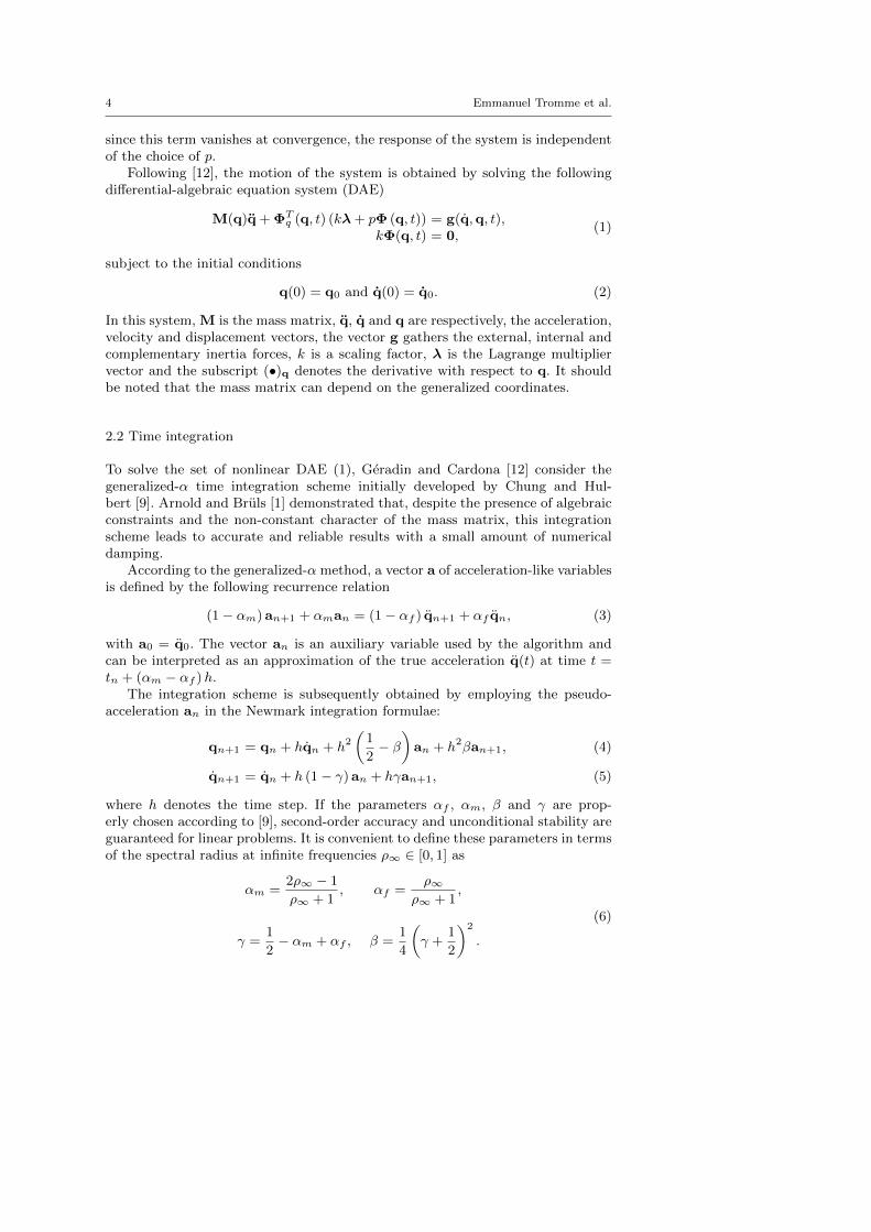
2.2 Time integration

To solve the set of nonlinear DAE (1), Geradin and Cardona [12] consider thegeneralized-α time integration scheme initially developed by Chung and Hul-bert [9]. Arnold and Bruls [1] demonstrated that, despite the presence of algebraicconstraints and the non-constant character of the mass matrix, this integrationscheme leads to accurate and reliable results with a small amount of numericaldamping.

According to the generalized-α method, a vector a of acceleration-like variablesis defined by the following recurrence relation

(1− αm) an+1 + αman = (1− αf ) qn+1 + αf qn, (3)

with a0 = q0. The vector an is an auxiliary variable used by the algorithm andcan be interpreted as an approximation of the true acceleration q(t) at time t =tn + (αm − αf )h.

The integration scheme is subsequently obtained by employing the pseudo-acceleration an in the Newmark integration formulae:

qn+1 = qn + hqn + h2(

1

2− β

)an + h2βan+1, (4)

qn+1 = qn + h (1− γ) an + hγan+1, (5)

where h denotes the time step. If the parameters αf , αm, β and γ are prop-erly chosen according to [9], second-order accuracy and unconditional stability areguaranteed for linear problems. It is convenient to define these parameters in termsof the spectral radius at infinite frequencies ρ∞ ∈ [0, 1] as

αm =2ρ∞ − 1

ρ∞ + 1, αf =

ρ∞ρ∞ + 1

,

γ =1

2− αm + αf , β =

1

4

(γ +

1

2

)2

.

(6)


The choice ρ∞ = 0 annihilates high frequency response whereas ρ∞ = 1 corre-sponds to no numerical damping.

At time step n + 1, the variables qn+1, qn+1, qn+1 and λn+1 must satisfythe system of nonlinear equations (1). To solve this dynamic equilibrium problem,a Newton-Raphson procedure associated with the linearized form (7) of (1) isemployed, which brings the residual of (1), i.e. r = Mq + ΦT

q (kλ+ pΦ)− g andΦ, close to zero. More precisely, around an approximate solution q, q, q, λ, thelinearized residual equations are solved

r (q +∆q, q +∆q, q +∆q,λ+∆λ) 'r (q, q, q,λ) + M∆q + Ct∆q + Kt∆q + ΦT

q (k∆λ+ pΦq∆q) = 0,kΦ (q +∆q) ' kΦ (q) + kΦq∆q = 0,

(7)

where Ct = ∂r/∂q and Kt = ∂r/∂q denote the tangent damping and tangentstiffness matrices respectively.

3 Weakly coupled approach - Equivalent static load method

3.1 Introduction and definition

In the context of dynamic response, the optimization problem formulation involvestime-dependent functions. The purpose of the equivalent static load method isto remove the time component from the problem, i.e. to transform the dynamicresponse optimization problem into a static optimization problem with multipleload cases [8]. Indeed, all the advantages of static response optimization and all thestandard methods can thus be used while the problems related to time-dependentfunctions are circumvented.

In [18], the authors define an equivalent static load as follows:Definition 1. When a dynamic load is applied to a structure, the equivalent staticload is defined as the static load that produces the same displacement field as theone created by the dynamic load at an arbitrary time.

In order to introduce the concept of equivalent static loads, let us considerthe following equilibrium equation of a linear structure1 subject to a dynamicload g (t)

M(p)q(p, t) + K(p)q(p, t) = g(t), (8)

where p is the design variable vector, q and q are the displacement and accelerationvectors respectively, and the damping effect is neglected. Terms of equation (8)can be rearranged as

K(p)q(p, t) = g(t)−M(p)q(p, t). (9)

The left-hand-side of (9) has a similar layout as the classical static equilibriumequation of a structure. By identification and according to the previous definition,the equivalent static load at time t is defined as

geq(t) = g(t)−M(p)q(p, t). (10)

1 The difference is made between a multibody system and a structure as the latter is com-posed of only one body. This enables a simplification of the equations for this introductorysection.


It should be noticed that the equivalent static load geq(t) is an implicit functionof the design variables and that it involves the external loads and inertia forces.From an analysis point of view, equivalent static loads seem useless but they aredeveloped in order to elaborate a static response optimization problem. In lieu ofconsidering the dynamic loading, they offer the possibility of considering a seriesof static loads that give at each time step the same displacement field as the onegiven by the dynamic loading. Therefore, the dynamic optimization problem istransformed into a optimization problem subject to multiple static load cases,with a load case for each integration time step.

3.2 Derivation of the equivalent static loads using a floating frame of referenceformalism

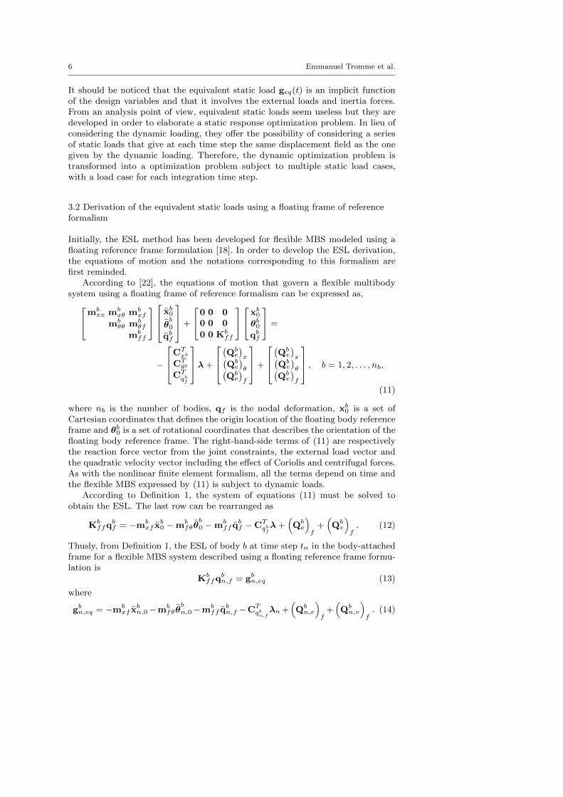
Initially, the ESL method has been developed for flexible MBS modeled using afloating reference frame formulation [18]. In order to develop the ESL derivation,the equations of motion and the notations corresponding to this formalism arefirst reminded.

According to [22], the equations of motion that govern a flexible multibodysystem using a floating frame of reference formalism can be expressed as,mb

xx mbxθ mb

xf

mbθθ mb

θf

mbff

xb0

θb0

qbf

+

0 0 00 0 0

0 0 Kbff

xb0θb0qbf

=

−

CTxb

CTθb

CTqbf

λ+

(Qbe

)x(

Qbe

)θ(

Qbe

)f

+

(Qbv

)x(

Qbv

)θ(

Qbv

)f

, b = 1, 2, . . . , nb,

(11)

where nb is the number of bodies, qf is the nodal deformation, xb0 is a set ofCartesian coordinates that defines the origin location of the floating body referenceframe and θb0 is a set of rotational coordinates that describes the orientation of thefloating body reference frame. The right-hand-side terms of (11) are respectivelythe reaction force vector from the joint constraints, the external load vector andthe quadratic velocity vector including the effect of Coriolis and centrifugal forces.As with the nonlinear finite element formalism, all the terms depend on time andthe flexible MBS expressed by (11) is subject to dynamic loads.

According to Definition 1, the system of equations (11) must be solved toobtain the ESL. The last row can be rearranged as

Kbffq

bf = −mb

xf xb0 −mb

fθθb0 −mb

ff qbf −CT

qbfλ+

(Qbe

)f

+(Qbv

)f. (12)

Thusly, from Definition 1, the ESL of body b at time step tn in the body-attachedframe for a flexible MBS system described using a floating reference frame formu-lation is

Kbffq

bn,f = gbn,eq (13)

where

gbn,eq = −mbxf x

bn,0−mb

fθθbn,0−mb

ff qbn,f −CT

qbn,fλn+

(Qbn,e

)f

+(Qbn,v

)f. (14)


In (14), the first two terms represent the effect of the coupling between rigid bodymotion and elastic deformation while the third term represents the inertia forcevector caused by elastic deformation of flexible bodies. The fourth term is thereaction force vector from the joint constraints, the fifth term is the external loadvector and the last term includes the effect of the Coriolis and centrifugal forces.

From the previous developments initially made by Kang et al. [18], it is ob-served that the resulting equations of motion resulting from the floating referenceframe formalism are suitable to obtain directly the ESL.

3.3 Derivation of the equivalent static loads using a nonlinear finite elementformalism

In [18], the derivation of the ESL for flexible MBS is straightforward due to in-herent properties of the floating reference frame formulation. First, we point outthat the stiffness matrix is constant in the body-attached frame during the entiremotion. Thusly, independently of the system configuration, a single stiffness ma-trix per body is considered in the optimization process, i.e. for all the time steps.Second, the component deformation is computed in the body-attached frame andis readily extracted for the ESL computation.

These essential characteristics do not exist in a standard nonlinear finite ele-ment formalism. The equations of motion are developed in an inertial frame, i.e.the forces are not expressed in a body-attached frame. Furthermore, no decouplingexists between rigid body motion and elastic deformation which is usually one ofits key point.

Hereafter, we propose a method to recover these characteristics in a post-processing step of the MBS simulation wherein ESL are obtained. We note thatthe proposed method does not alter the MBS analysis.

At a converged time step tn, linearizing the equations of motion (1) leads to

M∆q + Ct∆q + Kt∆q + ΦTq (k∆λ+ pΦq∆q) = ∆r,

kΦq∆q = ∆Φ.(15)

At first sight, it would be possible to obtain a similar expression as in (9). However,several problems are encountered when trying to apply Definition 1. Firstly, thetangent stiffness matrix is related to the whole system and it evolves with thesystem configuration. It would be very inefficient to store this matrix for eachtime step. Secondly, the body tangent stiffness matrix Kb

t of body b is neededto derive the ESL of body b. Thirdly, the generalized coordinate vector q(tn)exhibits no decoupling between rigid body motion and elastic deformation whilethe knowledge of deformation is required to derive ESL.

The key idea of the method is to introduce a corotational frame per body ina post-processing step so that the required characteristics can be recovered. Wenote that several definitions of the corotational frame exist such as e.g. a definitionbased on the minimization of the strain energy, a chord frame or a tangent framedefinition [29].

The above-mentioned problems are circumvented as follows. 1) A single tan-gent stiffness matrix for a chosen reference state Kt(tref ) is stored whereuponappropriate transformations must be applied to the vector q(tn) in order to bring


it back to the reference configuration for all other time steps. Based on the coro-tational frame, transformation rules can be established to switch from the actualconfiguration to the reference configuration and vice-versa. 2) For each body b,the body tangent stiffness matrix Kb

t(tref ) is extracted from Kt(tref ) of the ref-erence state. This is easily performed by identifying the coordinates related tothe nodes of body b and then extracting the body tangent stiffness matrix fromthe complete matrix. This technique is possible because, in our implementationof the finite element formalism, each body has its own set of nodal rotation andtranslation coordinates, which are not shared with other bodies. 3) Componentdeformation measure is defined with respect to the body-attached frame, i.e. thecorotational frame.

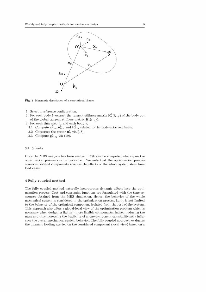
For each body b, a corotational frame definition is adopted and defined byxb0 and θb0, the position of the body-attached frame in the inertial frame andthe relative rotation vector of the body-attached frame compared to its referenceconfiguration. As illustrated in Figure 1, the relationship between the absoluteposition xi and orientation Ψi of node i of a flexible component and its localdisplacement ui and rotation ψi with respect to the corotational frame is givenby

xi = xb0 + Rb0 (Xi + ui) , (16)

Ψi = θb0 ◦ ψi, (17)

where Rb0(θb0) is the rotation matrix between the inertial frame and the coro-

tational frame, Xi is the position of node i in the body-attached frame for thenon-deformed configuration and the operation ◦ symbolizes the composition ofrotations. Amongst others, Cardona and Geradin [7] provide a comprehensive def-inition of corotational frames.

From (16)-(17), a local generalized displacement vector ubn with respect to thecorotational frame for body b at time step tn is defined as

ubn =[uT1 ψ

T1 . . .u

Ti ψ

Ti . . .u

Tnnψ

Tnn

]T, (18)

where nn numbers the nodes of body b. The size of the vector ubn is (nu + nψ)nn×1, where nu and nψ represent the dimension of the local displacement and rotationvectors, respectively. For planar problems, nu = 2 and nψ = 1 and for spatialproblems, nu = nψ = 3.

For MBS modeled using a standard nonlinear finite element formalism, theESL gbn,eq in the corotational frame at time tn for body b is defined as

gbn,eq = Kbt(tref )ubn. (19)

To solve (19), boundary conditions must be enforced to remove the stiffnessmatrix singularity caused by the rigid body modes. They mainly depends on thechoice of the corotational frame definition. For example, if a tangent frame isused at node i, the local displacement of node i should be zero, i.e. clampingconditions must be enforced in (19). A parallel reasoning can be drawn with thefloating reference frame formulation wherein boundary conditions must be imposedto components in order to introduce flexibility in the MBS analysis, see e.g. theComponent Mode Synthesis method [22].

In summary, to define ESL for MBS modeled using a standard nonlinear finiteelement formalism, five steps must be followed:


OE2

E3

E1

O′

x0

e1

e2e3

Xi

ui

xi

Fig. 1 Kinematic description of a corotational frame.

1. Select a reference configuration,2. For each body b, extract the tangent stiffness matrix Kb

t(tref ) of the body outof the global tangent stiffness matrix Kt(tref ),

3. For each time step tn and each body b,3.1. Compute xb0,n, θb0,n and Rb

0,n related to the body-attached frame,

3.2. Construct the vector ubn via (18),3.3. Compute gbn,eq via (19).

3.4 Remarks

Once the MBS analysis has been realized, ESL can be computed whereupon theoptimization process can be performed. We note that the optimization processconcerns isolated components whereas the effects of the whole system stem fromload cases.

4 Fully coupled method

The fully coupled method naturally incorporates dynamic effects into the opti-mization process. Cost and constraint functions are formulated with the time re-sponses obtained from the MBS simulation. Hence, the behavior of the wholemechanical system is considered in the optimization process, i.e. it is not limitedto the behavior of the optimized component isolated from the rest of the system.This approach also offers a global-local view of the optimization problem which isnecessary when designing lighter - more flexible components. Indeed, reducing themass and thus increasing the flexibility of a lone component can significantly influ-ence the overall mechanical system behavior. The fully coupled approach evaluatesthe dynamic loading exerted on the considered component (local view) based on a


global system-level simulation and the optimization process also accounts for thesystem global behavior.

With the fully coupled method, possibilities seem increased compared to anisolated component optimization approach since more complex and coupled behav-iors related to the whole system are considered. However, the optimization problemformulation should be carefully addressed to obtain good convergence [28].

5 Optimization of flexible multibody systems

5.1 Formulation of the MBS optimization problem

Engineering design problems can be formulated as a mathematical optimizationproblems (20) in which an objective function f0 (p) is minimized, subject to nc con-straints fj (p) ensuring the integrity of the structural design and design require-ments. The nv independent design variables are gathered in the vector p. Side-constraints p

i≤ pi ≤ pi reflect technological considerations.

minimizep

f0 (p)

subject to fj (p) ≤ f j , j = 1, . . . , nc,

pi≤ pi ≤ pi, i = 1, . . . , nv.

(20)

This formulation provides a general and robust design framework that can besolved by various types of optimization algorithms.

In MBS optimization, the cost and constraint functions are based on structuralproperties and responses, i.e. mass, displacement or stress measures at particularpoints and time steps. The design variables nv can be sizing, shape or topologicalvariables. Only sizing variables are considered here.

In the paper, the optimization problem concerns the minimization of the me-chanical system mass m(p) while constraints are enforced at each time step, i.e. alocal formulation of the constraints. This option offers a tight control over the op-timal design but the large number of constraints hinders the optimization process.Local formulations are usually opposed to global formulations which agglomerateparts or entire responses into a few constraints. The reduced number of constraintsgenerally facilitates the optimization convergence but the precise control of the op-timized design is relinquished due to their global nature. The complexity of thetreated examples is rather moderate so that basic local formulations are sufficient.

Particularizing the general formulation (20) to the MBS optimization consid-ered in this paper reads

minimizep

m (p)

subject to M(p)qn + ΦTq (p) (kλn + pΦ(p)) = g(p),

kΦ(p) = 0,

fj (p,qn, qn, qn,λn, tn) ≤ f j , j = 1, . . . , nc,

pi≤ pi ≤ pi, i = 1, . . . , nv,

(21)

for n = 1, . . . , nend, where nend is the number of simulation time steps.


We note that this formulation can easily be extended to account for globalconstraints of the form

nend∑k=1

fkj (p,qn, qn, qn,λn, tn) ≤ f j . (22)

5.2 Optimization algorithm and sensitivity analysis

Mathematical programming tools are used to solve the optimization problem (21).Gradient-based methods have been employed to solve large scale structural andmultidisciplinary optimization problems with great success [10, 24]. The majoradvantage of these methods is their good convergence rates which limits the num-ber of function evaluations to obtain an optimal design. However, these methodsare sensitive to local optima. In this study, we employ an “active-set” algorithmwhich is based on the sequential quadratic programming approach and is part ofthe optimization toolbox of Matlab® [17].

Gradient-based optimization methods require a sensitivity analysis to computethe derivatives of the cost and constraint functions. The efficiency of the sensitivityanalysis is an essential part of the optimization process because it can drasticallyaffect computation time. While a semi-analytical sensitivity analysis needs lesscomputational efforts in comparison to a finite difference scheme, the latter ap-proach is adopted in this paper. This sensitivity analysis requires one additionalsimulation per design variable and thus, CPU time grows by a factor nv + 1. How-ever, we adopt it to carry out the investigations as this method is easy to use andthe computation time is rather small for the examples considered here.

5.3 Weakly coupled method

Employing the weakly coupled method, the optimization problem formulation (21)is reformulated such that the dynamic response of the system is replaced by a se-ries of static responses, i.e. at time step tn, the component deformation under thedynamic loading is mimicked by an ESL. As proposed in [8], the optimization pro-cess repeatedly solves the following static response optimization problem whereinESL are incorporated,

minimizep

m (p)

subject to Kbt(p, tref )ubn = gbn,eq, b = 1, . . . nb,

fj(p,ubn, tn

)≤ f j , j = 1, . . . , nc,

pi≤ pi ≤ pi, i = 1, . . . , nv,

(23)

for n = 1, . . . , nend.In the optimization problem (23), the constraints are formulated with respect

to the local generalized displacement vector ubn, i.e. responses in the corotationalframe. To consider responses in the inertial frame, a relation must be definedto switch from the corotational frame to the inertial frame representation based


on (16)-(17). As shown afterwards in the examples, the constraints are often formu-lated as a function of qbn, i.e. f∗j

(p,qbn(ubn), tn

)≤ f∗j , where qbn is the generalized

coordinate vector related to body b at time step tn in the inertial frame defined as

qbn =[xT1 ΨT

1 . . .xTi ΨT

i . . .xTnnΨT

nn

]T. (24)

We note that after the first iteration of the static optimization process, theassembly of qbn for all bodies creates a global generalized coordinate vector whichdoes not respect the kinematic constraints anymore since each component hasbeen optimized independently.

In the optimization problem formulation (23), each body is loaded by as manyload cases as the number of time steps. During the static response optimizationprocess, the ESL are not updated. Therefore, cycles between MBS analysis andstatic response optimization are needed to account for the effects of the designmodification over the ESL. Reference [15] shows that doing so is identical to neglectthe time dependency in the sensitivity analysis of (21).

To solve the dynamic response optimization problem using the weakly coupledmethod, the algorithm proposed in [8], apart from the stopping criteria, is asfollows,

1. Initialize the design variables and set it = 0.2. Perform a dynamic MBS analysis.3. Compute the ESL.4. If it = 0, go to step 5. If it > 0 and if

tend∑n=1‖gbn,eq,it − gbn,eq,it−1‖

tend∑n=1‖gbn,eq,it−1‖

< ε, (25)

then, stop. Otherwise go to step 5.5. Solve the static response optimization problem (23). The iterations to solve

this optimization problem are hereafter denoted as inner iterations.6. Set it = it+ 1 and go to step 2.

One cycle is composed of steps 2 to 6. Reference [26] discusses the convergenceof the solution obtained using this optimization method towards the optimal so-lution of the original dynamic response optimization problem. Figure 2 illustratesthe flowchart of the ESL method.

5.4 Fully coupled method

Considering the fully coupled method, the optimization problem formulation (21)is employed as it is. The flowchart of the optimization process is illustrated inFigure 3. The MBS simulation and the optimization process are fully coupled,i.e. at each iteration of the optimization process, a MBS analysis is performed.However, as described in Section 4, the design problem is quite complex and theconvergence may suffer poor properties if not treated properly. This is due to theexistence of significant couplings between vibrations and large amplitude motions,


1

ESL computation

MBS analysis

Initial design

ConvergenceESL?

Static responseoptimization

(Inner iterations)

Design updateit = it + 1

StopYes

No

Fig. 2 Flowchart of the weakly coupled method.

the influence of the changes of component inertial property on the vibrations aswell as the interactions between flexible components.

Using the fully coupled method, the sensitivity analysis can be costly if not ad-dressed with care. Efficient semi-analytical sensitivity methods have been proposedto compute the response derivatives, i.e. dqn/dp, dqn/dp, dqn/dp, dλn/dp [3, 4].The sensitivity analysis can also be incorporated into the time integration schemeof the MBS analysis whereupon the cost of gradient computation is significantlylessened.

1

MBS analysis+

Sensitivity analysis

Initial design

Convergence?

Dynamic responseOptimization

Design updateit = it + 1

StopYes

No

Fig. 3 Flowchart of the fully coupled method.


6 Optimization of 2-dof planar robot

6.1 Modeling hypotheses

The first example concerns the mass minimization of a 2-dof planar robot inspiredfrom [18, 19]. Each robot arm has a length of 600 mm and is modeled by twoequal length beam elements with a hollow cross section (Fig. 4(a)). The adoptedbeam element model is described in [12]. The robot is made of aluminum witha Young’s modulus of E = 72 GPa, Poisson’s ratio of ν = 0.3 and mass densityof 2700 kg/m3. Each revolute joint is driven by an ideal motor which imposesa smooth joint trajectory θ1(t) and θ2(t) such that the robot tip deploys alonga straight line. The initial joint angles are θ1(t0) = 120◦ and θ2(t0) = −150◦.The ideal (rigid MBS) tip displacement corresponds to the following trajectoryequation

∆xtip(t) = ∆ytip(t) =0.5

T

(t− T

2πsin

2πt

T

), (26)

where the period of the deployment motion T is set to 0.5 s.

The actuator of the second robot arm is located at joint A and has a mass of2 kg. The combined mass of the end-effector plus the payload is 1 kg. The gravityfield is considered. The simulation is performed using the generalized-α schemewith a time step h = 5× 10−4 s and a spectral radius of ρ∞ = 0.5.

The design variables pi are the outer diameters of the hollow beam elementswhose wall thickness is set to 0.1 × pi. Initial values of the design variables areset to 50 mm. Tangent corotational frames are adopted to derive the ESL. Thusly,the boundary conditions of each static load case correspond to fixed-free beamconditions.

p1

p2p3

p4

x

y

θ2(t)

θ1(t)

A

Tip

gravity

(a) Kinematic model of the 2-dof robot.

x

y

yAr

yA

ytiprytip

(b) Deflection constraint notation.

Fig. 4 Modeling of the 2-dof robot.

The optimization problem concerns the mass minimization of the robot m (p)subject to nc deviation constraints ∆l(p,qn, tn) where nc equals the number of


integration time steps. Mathematically, it is stated as

minimizep

m (p)

subject to ∆l(p,qn, tn) ≤ ∆l, n = 1, . . . , nend,

0.02 m ≤ pi ≤ 0.06 m, i = 1, . . . , 4.

(27)

Two different optimization problems are studied hereafter, which result from twodifferent formulations of the deviation constraints.

6.2 Component-based constraints

Inspired from the initial paper [18] considering the coupling between the ESLmethod and flexible MBS, the deviation constraint at time step tn reads

∆l =

√(yA − yAr

)2 + ((ytip − ytipr )− (yA − yAr))2 ≤ 0.001 m (28)

where yA and ytip are respectively the joint A and tip y-positions in the inertialframe (Fig. 4(b)) and the subscript r refers to a reference mechanism, here thesame mechanism but whose components are modeled as rigid bodies.

The constraint formulation (28) is not suitable to perform the optimizationproblem using the weakly coupled method as the terms are related to values inthe inertial frame while the weakly coupled method makes use of values in thebody-attached frame. Based on (16)-(17), (28) is easily reformulated as

∆l =

√(R1

0,nu1n,A

∣∣∣y

)2

+(

R20,nu2

n,tip

∣∣y

)2≤ 0.001 m, (29)

which only contains values related to the body-attached frames. Formulation (28)is employed with the fully coupled method.

The simulation time interval is 0.65 s corresponding to 1301 time steps. Thefully coupled method is deemed converged when the relative change of the objectivefunction value and the relative constraint violation are less than 10−3 and 10−6

respectively. The weakly coupled method is deemed converged when the stoppingcriteria (25) with ε equals to 10−2 is satisfied. These stopping criteria ensure a tightconvergence of the optimization processes so that the comparison is performed onconverged solutions.

The optimization results are gathered in Table 1 and the convergence historyis illustrated in Figure 5. For readability reasons of this figure, markers are printedeach 0.01 s. It is observed that both optimization methods converge quickly to-wards a similar optimal design. The fully coupled method has no inner iterationcompared to the weakly coupled method. However, the inner iterations are basedon static computations and static analyses are less CPU-time consuming than dy-namic analyses. Moreover, in this example, the weakly coupled method needs lessglobal iterations, i.e. MBS analysis, to converge. However it is not easy to draw ageneral conclusion about the relative efficiency of the two methods in this case.


Table 1 Numerical results (in kg and mm) - 2-dof robot - formulation (28).

Method Mass Iter. Inner p1 p2 p3 p4iter.

Weakly Coupled 0.962 6 57 39.29 28.33 34.94 25.19Fully Coupled 0.962 9 / 39.35 28.25 35.14 24.91

0 2 4 6 8 100

0.5

1

1.5

2

2.5

3

Iterations

MassEvolution

[kg]

Weakly C.M.Fully C.M.

0 0.1 0.2 0.3 0.4 0.5 0.6 0.70

0.2

0.4

0.6

0.8

1

1.2

Time [s]

Deviation

Con

straint[m

m]

Upper bound

1

Fig. 5 2-dof robot - formulation (28): objective function history and deviation constraint forthe optimal design.

6.3 Multicomponent-based constraints

In [19], the authors enforce a trajectory tracking constraint which is expressed attime step tn as

∆l =

√(xtip − xtipr )2 + (ytip − ytipr )2 ≤ 0.001 m (30)

where xtip and ytip are respectively the tip x and y-positions in the inertial frame.The simulation time interval is still equals to 0.65 s. Stopping criteria are identicalto the ones used in Section 6.2.

In the previous example, each optimized component is subject to component-based constraints, i.e. each component is constrained by its own responses. Here,the trajectory tracking constraint enforces a multicomponent-based constraint,i.e. by constraining the absolute deflection of the robot tip, all components areconstrained. However, the weakly coupled method concerns the optimization ofcomponents which are isolated from the rest of the system during the optimizationprocess. Thusly, (30) must be reformulated in order to consider the flexibility ofthe whole system by enforcing component-based constraints.

Due to the open-loop system properties, we formulate the deflection of thetip as a linear combination of all the component deflections. At time step tn, thedeflection of the tip is stated as[

xtip − xtiprytip − ytipr

]=

nb∑k=1

Rk0,nukn,ext (31)


where k is the robot link index and the subscript ext denotes the link extremity.

Using the fully coupled method, multicomponent-based constraints are incor-porated in the optimization problem without any difficulty. The generalized coordi-nates of the MBS analysis are available for the optimization process and naturallyaccount for the flexibility of the whole mechanism.

The optimization results are given in Table 2 and are illustrated in Figure 6.Markers are again printed each 0.01 s. The weakly coupled method is deemedconverged after 5 cycles while the fully coupled needs 11 iterations. Although theoptimal values of objective functions are similar, the design variable values areslightly different. The effect is observed in Figure 6 where the time responses ofthe optimal systems are different. However, the critical time zone around 0.1 sexhibits not so much difference between the two optimal solutions in terms of timeresponse.



Weakly Coupled 1.411 5 49 47.87 34.51 42.11 30.08Fully Coupled 1.408 11 / 48.58 35.02 41.43 29.08

0 2 4 6 8 101

1.2

1.4

1.6

1.8

2

2.2

2.4

Iterations

MassEvolution

[kg]


0 0.1 0.2 0.3 0.4 0.5 0.6 0.70

0.2

0.4

0.6

0.8

1

1.2

Time [s]

Deviation

Con

straint[m

m]

Upper bound

1

Fig. 6 2-dof robot - formulation (30): objective function history and deviation constraint forthe optimal design.


7 Optimization of a 4-bar mechanism

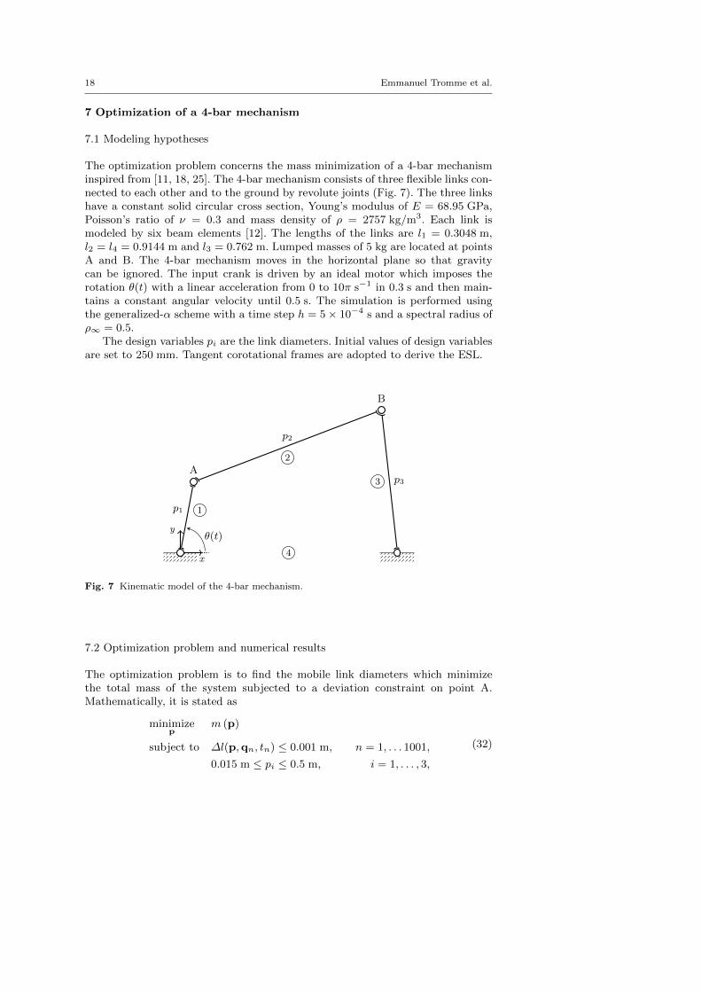
7.1 Modeling hypotheses

The optimization problem concerns the mass minimization of a 4-bar mechanisminspired from [11, 18, 25]. The 4-bar mechanism consists of three flexible links con-nected to each other and to the ground by revolute joints (Fig. 7). The three linkshave a constant solid circular cross section, Young’s modulus of E = 68.95 GPa,Poisson’s ratio of ν = 0.3 and mass density of ρ = 2757 kg/m3. Each link ismodeled by six beam elements [12]. The lengths of the links are l1 = 0.3048 m,l2 = l4 = 0.9144 m and l3 = 0.762 m. Lumped masses of 5 kg are located at pointsA and B. The 4-bar mechanism moves in the horizontal plane so that gravitycan be ignored. The input crank is driven by an ideal motor which imposes therotation θ(t) with a linear acceleration from 0 to 10π s−1 in 0.3 s and then main-tains a constant angular velocity until 0.5 s. The simulation is performed usingthe generalized-α scheme with a time step h = 5× 10−4 s and a spectral radius ofρ∞ = 0.5.

The design variables pi are the link diameters. Initial values of design variablesare set to 250 mm. Tangent corotational frames are adopted to derive the ESL.

p1 1

p2

2

p33

4x

y

A

B

θ(t)

Fig. 7 Kinematic model of the 4-bar mechanism.

7.2 Optimization problem and numerical results

The optimization problem is to find the mobile link diameters which minimizethe total mass of the system subjected to a deviation constraint on point A.Mathematically, it is stated as

minimizep

m (p)

subject to ∆l(p,qn, tn) ≤ 0.001 m, n = 1, . . . 1001,

0.015 m ≤ pi ≤ 0.5 m, i = 1, . . . , 3,

(32)


where at time step tn,

∆l =

√(xA − xAr

)2 + (yA − yAr)2. (33)

In (33), xA and yA are respectively the x and y-positions of point A in the inertialframe. The reference mechanism is the same mechanism but whose componentsare modeled as rigid bodies. The optimization differs from [11, 18, 25] whereinauthors consider stress constraints.

The weakly coupled method can hardly incorporate the loop closure kinematicin the optimization problem formulation due to the component-based characteris-tics of the method. To overcome this difficulty, the closed-loop system is opened inthe optimization problem formulation and the multicomponent-based constraintis split into two constraints. The first one enforces a limit on the deflection of link1 and the second one constrains the cumulative deflection of links 2 and 3. At timetn and using the values related the body-attached frames, it reads

∆l1 =

((R1

0,nu1n,A

∣∣∣x

)2+

(R1

0,nu1n,A

∣∣∣y

)2) 1

2

≤ 0.001 m, (34)

∆l2 =

((R2

0,nu2n,A

∣∣∣x

+ R30,nu3

n,B

∣∣∣x

)2+

.

(R2

0,nu2n,A

∣∣∣y

+ R30,nu3

n,B

∣∣∣y

)2) 1

2

≤ 0.001 m, (35)

where the last subscript of ubn denotes the point where the displacement is consid-ered. Note that the loop closure constraint is still enforced in the MBS simulation,it is only discarded at the level of the optimization procedure. On the contrario,the fully coupled method incorporates constraint (33) without any difficulty.

The fully coupled method is deemed converged when the relative changes of theobjective function value and design variable values vary less than 10−3 while therelative constraint violation is less 10−6. The weakly coupled method is deemedconverged when the stopping criteria (25) with ε equals to 10−2 is satisfied. Thesetolerance values ensure a tight convergence of the optimization processes so thatthe comparison is performed on converged solutions.

The initial design has a mass of 268 kg (without the lumped masses) anda maximum deviation around 50 µm which is far from the upper bound limit.The optimal design greatly differs depending on the optimization method. Theobjective function optimal value is 7 times larger with the weakly coupled method(Tab. 3). The ESL method surprisingly needs a large number of iterations toconverge. In Figure 8, it is observed that, in both methods, at least one constraintis active once converged. The optimization processes would seem to be trapped inlocal optima.

7.3 Trivial optimization

In order to explain the previously obtained behavior, the same optimization processis performed but the lumped masses at points A and B are removed.


Table 3 Numerical results (in kg and mm) - 4-bar mechanism.

Method Mass Iter. Inner p1 p2 p3iter.

Weakly Coupled 20.703 73 786 69.85 87.61 37.22Fully Coupled 2.967 21 / 56.15 15.10 16.24

0 10 20 30 40 50 60 70 800

50

100

150

200

250

300

Iterations

MassEvolution

[kg]


0 0.1 0.2 0.3 0.4 0.50

0.2

0.4

0.6

0.8

1

1.2

Time [s]

Deviation

Con

straint[m

m]

Upper bound

1

Fig. 8 4-bar mechanism: objective function history and deviation constraint for the optimaldesign.

Before performing the optimization, let us get a feeling of the optimal design.The goal is to minimize the deviation of point A which is mainly guided by themotor through link 1. Links 2 and 3 mainly follow the imposed motion and producereactions forces at point A. Thusly, physical intuition would tend to remove theselinks.

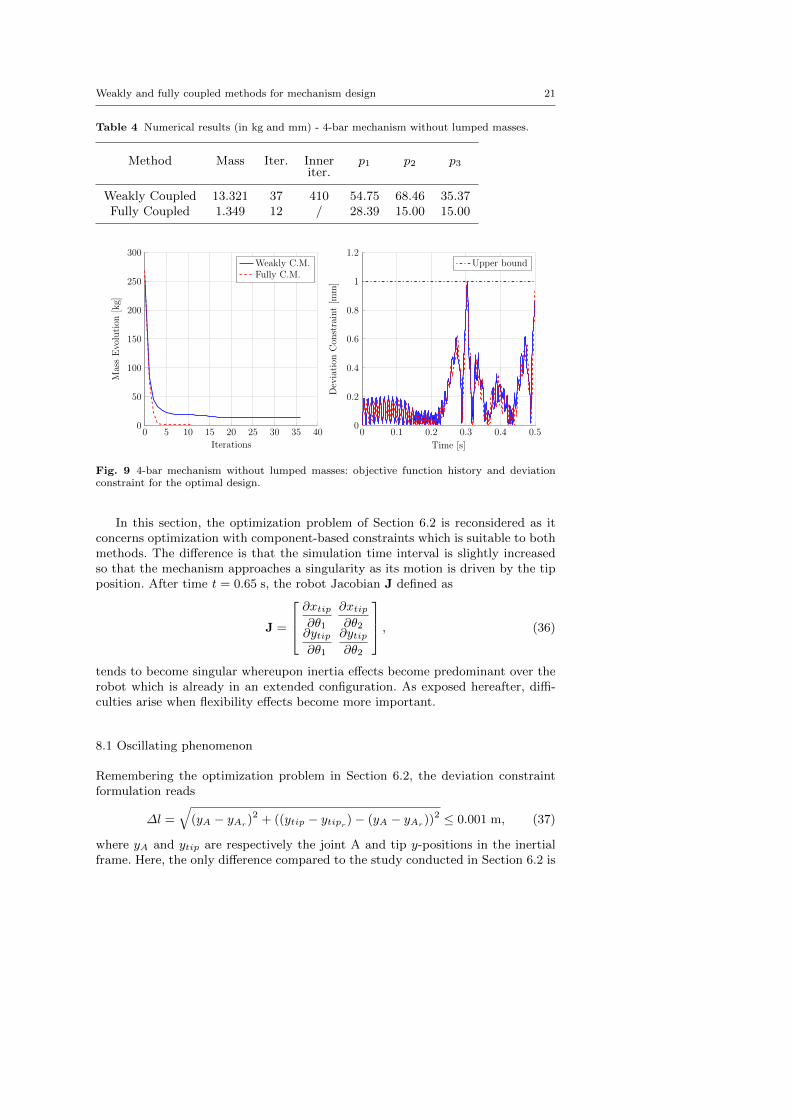
The optimization results are gathered in Table 4 and the convergence history isillustrated in Figure 9. The fully coupled method converges towards our predicteddesign wherein design variables p2 and p3 reach the lower bound of their side-constraints. The weakly coupled method also converges and at least one constraintis active at convergence but the optimum design is quite different. Links 2 and3 can not be removed, they are optimized in order to satisfy (35). However, ifthis constraint is suppressed, links 2 and 3 can no more be incorporated in theoptimization problem. This example illustrates that the weakly coupled is notsuitable to consider multicomponent-based constraints in the presence of closed-loops.

8 On some particular behaviors

The 2-dof robot example developed in the previous section concerns the structuraloptimization of mechanical systems wherein flexibility effects are not predominant.We have illustrated that both optimization methods can converge towards the sameoptimal design.


Table 4 Numerical results (in kg and mm) - 4-bar mechanism without lumped masses.

Method Mass Iter. Inner p1 p2 p3iter.

Weakly Coupled 13.321 37 410 54.75 68.46 35.37Fully Coupled 1.349 12 / 28.39 15.00 15.00

0 5 10 15 20 25 30 35 400

50

100

150

200

250

300

Iterations

MassEvolution

[kg]


0 0.1 0.2 0.3 0.4 0.50

0.2

0.4

0.6

0.8

1

1.2

Time [s]

Deviation

Con

straint[m

m]

Upper bound

1

Fig. 9 4-bar mechanism without lumped masses: objective function history and deviationconstraint for the optimal design.

In this section, the optimization problem of Section 6.2 is reconsidered as itconcerns optimization with component-based constraints which is suitable to bothmethods. The difference is that the simulation time interval is slightly increasedso that the mechanism approaches a singularity as its motion is driven by the tipposition. After time t = 0.65 s, the robot Jacobian J defined as

J =

∂xtip∂θ1

∂xtip∂θ2

∂ytip∂θ1

∂ytip∂θ2

, (36)

tends to become singular whereupon inertia effects become predominant over therobot which is already in an extended configuration. As exposed hereafter, diffi-culties arise when flexibility effects become more important.

8.1 Oscillating phenomenon

Remembering the optimization problem in Section 6.2, the deviation constraintformulation reads

∆l =

√(yA − yAr

)2 + ((ytip − ytipr )− (yA − yAr))2 ≤ 0.001 m, (37)

where yA and ytip are respectively the joint A and tip y-positions in the inertialframe. Here, the only difference compared to the study conducted in Section 6.2 is


that the simulation time interval is set to 0.66 s corresponding to 1321 time steps.The same stopping criteria are used.

The convergence history of the weakly coupled method is illustrated in Fig-ure 10. It is observed that the objective function value oscillates, which preventsthe convergence of the optimization and it reaches the allowed maximum numberof iterations. Observing the trajectory tracking constraint evolution during severaliterations (Fig. 10(b)-10(e)), we point out that the deviation constraint is alwaysactivated for the last time step but oscillating phenomenon appears due to thedeviation constraint around 0.125 s. Between iterations 4 and 5, the optimizationprocess reduces the mass and then tries to converge. However, after performing theMBS analysis and updating the ESL, the optimization process converge towardsa design that was previously obtained so that the process enters an infinite loop.Move-limits can be implemented to damp out these oscillations but the optimaldesign is thus artificially forced.

This example illustrates that in certain circumstances, oscillations prevent theoptimization convergence. However, in the present case, this phenomenon seemsto appear only for this particular simulation time interval where there is a stronginteraction between the activation of the constraint at the last time step and theactivation of constraints around 0.125 s.

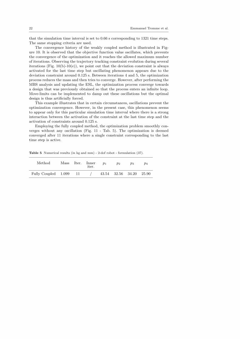
Employing the fully coupled method, the optimization problem smoothly con-verges without any oscillation (Fig. 11 - Tab. 5). The optimization is deemedconverged after 11 iterations where a single constraint corresponding to the lasttime step is active.



Fully Coupled 1.099 11 / 43.54 32.56 34.20 25.90


0 10 20 30 40 501

1.2

1.4

1.6

1.8

2

2.2

2.4

Iterations

MassEvolution

[kg]

1

(a) Objective function.

0 0.1 0.2 0.3 0.4 0.5 0.6 0.70

0.2

0.4

0.6

0.8

1

1.2

Time [s]

Deviation

Con

straint[m

m]

1

(b) Iteration 4.

0 0.1 0.2 0.3 0.4 0.5 0.6 0.70

0.2

0.4

0.6

0.8

1

1.2

Time [s]

Deviation

Con

straint[m

]

1

(c) Iteration 5.

0 0.1 0.2 0.3 0.4 0.5 0.6 0.70

0.2

0.4

0.6

0.8

1

1.2

Time [s]

Deviation

Con

straint[m

]

1

(d) Iteration 6.

0 0.1 0.2 0.3 0.4 0.5 0.6 0.70

0.2

0.4

0.6

0.8

1

1.2

Time [s]

Deviation

Con

straint[m

]

1

(e) Iteration 7.

Fig. 10 Weakly coupled method: illustration of the oscillating behavior of the optimizationprocess.


0 2 4 6 8 101

1.2

1.4

1.6

1.8

2

2.2

2.4

Iterations

MassEvolution

[kg]

Fully C.M.

0 0.1 0.2 0.3 0.4 0.5 0.6 0.70

0.2

0.4

0.6

0.8

1

1.2

Time [s]Deviation

Con

straint[m

m]

Upper bound

1

Fig. 11 2-dof robot - fully coupled method - formulation (37): objective function history anddeviation constraint for the optimal design.

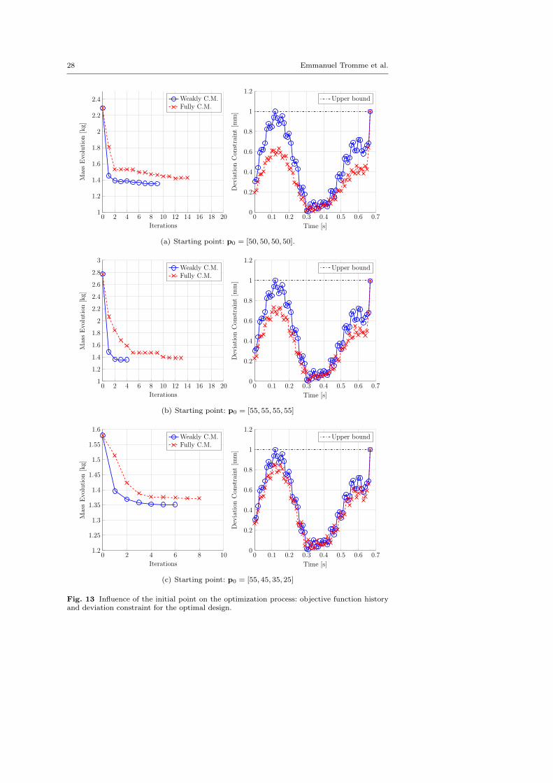
8.2 Initial point influence

A general characteristic of gradient-based algorithms is that they are sensitive tolocal optima. Thusly, depending on the initial value of design variables, severaloptimal designs can be obtained.

In this section, four different starting points are used: p10 = [50, 50, 50, 50],

p20 = [55, 55, 55, 55], p3

0 = [55, 45, 35, 25] and p40 = [45, 45, 45, 45]. The latter is an

infeasible starting point making the optimization process more complex.Considering the optimization problem treated in Section 6.2 and based on the

numerical results gathered in Table 6, we conclude that the influence of the initialpoint on the optimal design is not significant. To support this conjecture, thedeviation constraint is given as a function of the design parameters in Figure 12for time t = 0.0995 s where p1 and p3 are set to 39.35 and 35 mm respectively.The design domain presents similar shape for time steps around. It is observedthat the design space domain is relatively smooth whereupon the convergence isfacilitated and the optimization process is not much sensitive to local optima.

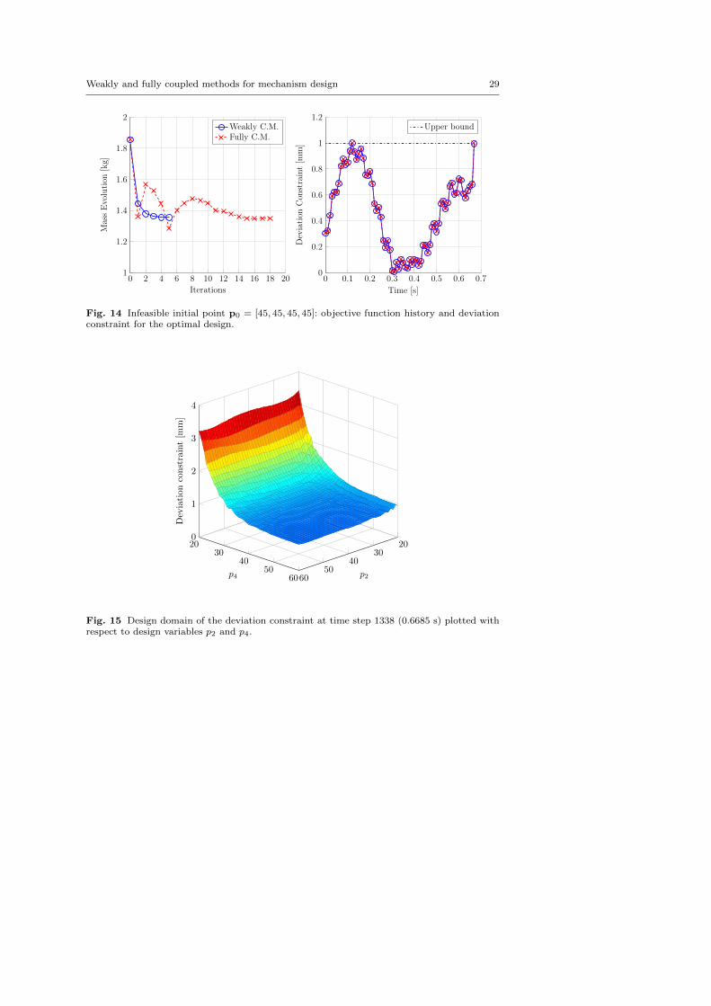
Let us now continue with the same optimization problem except that the 2-dof robot undergoes a motion until the final joint angles θ1(tend) = 60◦ andθ2(tend) = −30◦ corresponding to a simulation time interval of 0.6687 s and thus1338 time steps. Approaching the singularity of the mechanism, inertia effectsbecome more important.

Analyzing the results given in Table 7, the weakly coupled method seems to berather insensitive to the starting points. Although the number of iterations neededto converge strongly varies, the optimal design remains similar. Using the fullycoupled method, optimal designs differ with the initial points. Unlike the weaklycoupled method, in Figures 13-14, it is observed that the fully coupled methodgenerally activates only the constraint related to the last time step at convergence.In Table 8, the history of active constraints is given for p0 = [55, 55, 55, 55] whereit is clearly shown that the fully coupled method is more affected by the dynamic


Table 6 Formulation (28) - Numerical results for 4 initial points (in kg and mm).

Initial point Mass Iter. Inner p1 p2 p3 p4iter.

Weakly Coupled Method

p0 = [50, 50, 50, 50] 0.962 6 57 39.29 28.33 34.94 25.19p0 = [55, 55, 55, 55] 0.962 8 73 39.29 28.32 34.93 25.20p0 = [55, 45, 35, 25] 0.962 6 49 39.30 28.34 34.94 25.17p0 = [45, 45, 45, 45] 0.962 5 39 39.31 28.30 34.88 25.26

Fully Coupled Method

p0 = [50, 50, 50, 50] 0.962 9 / 39.35 28.25 35.14 24.91p0 = [55, 55, 55, 55] 0.962 11 / 39.39 28.19 35.15 24.91p0 = [55, 45, 35, 25] 0.961 16 / 39.36 28.24 35.10 24.88p0 = [45, 45, 45, 45] 0.962 9 / 39.46 28.17 35.10 24.84

2030

4050

60

2030

4050

60

0.8

1

1.2

1.4

p2p4

Deviation

constraint[m

m]

1

Fig. 12 Design domain of the deviation constraint at time step 200 (0.0995 s) plotted withrespect to design variables p2 and p4.

effects occurring at the end of the simulation. Using the weakly coupled method,the optimization is less affected by the last time step and as depicted in Table 8,the last constraint is no more active at convergence within the given tolerance.This behavior can be explained by the fact that design sensitivies are smootherin the weakly coupled method due to their time independence. In this case, thisapproximation avoids getting stuck in a local minimum created by the last timesteps where inertia effects are predominant.


To explain the difference between optimal designs obtained with the fully cou-pled method, the design space domain of the deviation constraint as a function ofdesign variables for time step t = 0.6685 s is illustrated in Figure 15 where p1 andp3 are set to 52.49 and 33.24 mm respectively. The design space configuration ex-hibits a lot of oscillations near the upper bound value of the constraint preventingthe convergence towards a unique optimal design.

Lastly, observing Figure 14, the convergence history exhibits oscillations. Thisis expected as the convergence is hardened when the starting point is infeasiblecombined with a local formulation of the optimization problem [28]. Other formu-lations can help to work with a feasible domain of the design space more adaptedto gradient-based algorithms but these difficult and important issues are left forfuture work.

Table 7 Influence of the initial point on the optimal design (in kg and mm).

Initial point Mass Iter. Inner p1 p2 p3 p4iter.

Weakly Coupled Method

p0 = [50, 50, 50, 50] 1.353 10 101 52.53 37.81 33.24 24.76p0 = [55, 55, 55, 55] 1.355 5 34 52.62 37.81 33.23 24.77p0 = [55, 45, 35, 25] 1.352 7 64 52.45 37.84 33.21 24.80p0 = [45, 45, 45, 45] 1.355 6 50 52.60 37.85 33.23 24.76

Fully Coupled Method

p0 = [50, 50, 50, 50] 1.427 15 / 51.71 36.89 38.07 27.31p0 = [55, 55, 55, 55] 1.386 14 / 51.82 36.77 36.90 25.52p0 = [55, 45, 35, 25] 1.372 9 / 52.27 37.32 34.24 26.32p0 = [45, 45, 45, 45] 1.350 19 / 52.85 37.21 33.29 24.66

9 Conclusions

Two optimization methods for the structural optimization of mechanisms havebeen compared. On the one hand, the weakly coupled method uses a MBS simu-lation to generate ESL whereupon static response optimization with multiple loadcases is performed. On the other hand, the fully coupled method solves a dynamicresponse optimization problem with time responses obtained directly from theMBS analysis.

In order to carry out a fair comparison using an unique MBS formalism, weproposed a method to derive ESL adapted to a standard nonlinear finite elementformulation.

When the optimization problem concerns component-based constraints, i.e.where each component is optimized subject to its own set of constraints, bothmethods can converge towards the same optimum. The weakly coupled methodgenerally lessen the CPU time consumption as it avoids the expensive gradient


Table 8 History of active constraints, p0 = [55, 55, 55, 55].

Iterations Weakly coupled method Fully coupled method

1 / /2 1338 /3 286, 287, 288, 289, 290, 1338 /4 238, 239, 240, 241, 242, 1338 /5 239, 240, 241, 242 /6 - Conv - 1338...

...10 133811 /12 /13 /14 1338

computation of the state variables. Also, less dynamic analyses are usually requiredto converge. However, this reduction is partly balanced by inner iterations whichare performed at each cycle although the latter are based on static computations.

When multicomponent-based constraints are considered, the weakly coupledmethod is not suitable except in particular cases, i.e. when the multicomponent-based constraints can be properly translated into components-based constraints.The fully coupled method is more general and accommodates all types of com-ponent and multicomponent-based constraints at the price of a more complexoptimization process.

The examples illustrate the potential of both methods to perform structuraloptimization of flexible mechanisms. However, as illustrated by the last section, it isnot trivial to obtain convergence for mechanisms wherein flexibility and vibrationsare important. The understanding of the physical behavior of the mechanism isfundamental to manage the optimization process and interpret afterwards theoptimization results.

Acknowledgements Parts of this research have been supported by the LIGHTCAR Projectsponsored by the pole of competitiveness “MecaTech” and the Walloon Region of Belgium(Contract RW-6500) and the CIMEDE 2 Project sponsored by the pole of competitiveness“GreenWin” and the Walloon Region of Belgium (Contract RW-7179).


0 2 4 6 8 10 12 14 16 18 201

1.2

1.4

1.6

1.8

2

2.2

2.4

Iterations

MassEvolution

[kg]


0 0.1 0.2 0.3 0.4 0.5 0.6 0.70

0.2

0.4

0.6

0.8

1

1.2

Time [s]Deviation

Con

straint[m

m]

Upper bound

1

(a) Starting point: p0 = [50, 50, 50, 50].

0 2 4 6 8 10 12 14 16 18 201

1.2

1.4

1.6

1.8

2

2.2

2.4

2.6

2.8

3

Iterations

MassEvolution

[kg]


0 0.1 0.2 0.3 0.4 0.5 0.6 0.70

0.2

0.4

0.6

0.8

1

1.2

Time [s]

Deviation

Con

straint[m

m]

Upper bound

1

(b) Starting point: p0 = [55, 55, 55, 55]

0 2 4 6 8 101.2

1.25

1.3

1.35

1.4

1.45

1.5

1.55

1.6

Iterations

MassEvolution

[kg]


0 0.1 0.2 0.3 0.4 0.5 0.6 0.70

0.2

0.4

0.6

0.8

1

1.2

Time [s]

Deviation

Con

straint[m

m]

Upper bound

1

(c) Starting point: p0 = [55, 45, 35, 25]

Fig. 13 Influence of the initial point on the optimization process: objective function historyand deviation constraint for the optimal design.


0 2 4 6 8 10 12 14 16 18 201

1.2

1.4

1.6

1.8

2

Iterations

MassEvolution

[kg]


0 0.1 0.2 0.3 0.4 0.5 0.6 0.70

0.2

0.4

0.6

0.8

1

1.2

Time [s]Deviation

Con

straint[m

m]

Upper bound

1

Fig. 14 Infeasible initial point p0 = [45, 45, 45, 45]: objective function history and deviationconstraint for the optimal design.

2030

4050

60

2030

4050

60

0

1

2

3

4

p2p4

Deviation

constraint[m

m]

1

Fig. 15 Design domain of the deviation constraint at time step 1338 (0.6685 s) plotted withrespect to design variables p2 and p4.


References

1. Arnold, M., Bruls, O.: Convergence of the generalized-α scheme for constrainedmechanical systems. Multibody Systems Dynamics 18(2), 185–202 (2007)

2. Bendsøe, M., Sigmund, O.: Topology optimization: Theory, Methods, and Ap-plications. Springer Verlag, Berlin (2003)

3. Bestle, D., Seybold, J.: Sensitivity analysis of constrained multibody systems.Archive of Applied Mechanics 62, 181–190 (1992)

4. Bruls, O., Eberhard, P.: Sensitivity analysis for dynamic mechanical systemswith finite rotations. International Journal for Numerical Methods in Engi-neering 74(13), 1897–1927 (2008)

5. Bruls, O., Lemaire, E., Duysinx, P., Eberhard, P.: Optimization of multibodysystems and their structural components. In: Multibody Dynamics: Compu-tational Methods and Applications, vol. 23, pp. 49–68. Springer (2011)

6. Bruns, T., Tortorelli, D.: Computer-aided optimal design of flexible mecha-nisms. In: Proceedings of the Twelfth Conference of the Irish ManufacturingCommitee, IMC12, Competitive Manufacturing. University College Cork, Ire-land (1995)

7. Cardona, A., Geradin, M.: Modelling of superelements in mechanism analysis.International Journal for Numerical Methods in Engineering 32(8), 1565–1593(1991)

8. Choi, W., Park, G.: Structural optimization using equivalent static loads atall time intervals. Computer Methods in Applied Mechanics and Engineering191(19-20), 2105 – 2122 (2002)

9. Chung, J., Hulbert, G.: A time integration algorithm for structural dynamicswith improved numerical dissipation: The generalized-α method. Journal ofapplied mechanics 60, 371–375 (1993)

10. Deaton, J., Grandhi, R.: A survey of structural and multidisciplinary con-tinuum topology optimization: post 2000. Structural and MultidisciplinaryOptimization 49(1), 1–38 (2014)

11. Etman, L., Van Campen, D., Schoofs, A.: Design optimization of multibodysystems by sequential approximation. Multibody System Dynamics 2(4), 393–415 (1998)

12. Geradin, M., Cardona, A.: Flexible Multibody Dynamics: A Finite ElementApproach. John Wiley & Sons, New York (2001)

13. Haussler, P., Emmrich, D., Muller, O., Ilzhofer, B., Nowicki, L., Albers, A.: Au-tomated topology optimization of flexible components in hybrid finite elementmultibody systems using ADAMS/Flex and MSC.Construct. In: Proceedingsof the 16th European ADAMS Users’ Conference (2001)

14. Haussler, P., Minx, J., Emmrich, D.: Topology optimization of dynamicallyloaded parts in mechanical systems: Coupling of MBS, FEM and structuraloptimization. In: Proceedings of NAFEMS Seminar Analysis of Multi-BodySystems Using FEM and MBS. Wiesbaden, Germany (2004)

15. Held, A.: On structural optimization of flexible multibody systems. Ph.D. the-sis, Institut fur Technische und Numerische Mechanik, Universitat Stuttgart(2014)

16. Hong, E., You, B., Kim, C., Park, G.: Optimization of flexible componentsof multibody systems via equivalent static loads. Structural MultidisciplinaryOptimization 40, 549–562 (2010)


17. The MathWorks, Inc.: MATLAB and Optimization Toolbox Release 2012b.Natick, Massachusetts, United States. (2012)

18. Kang, B., Park, G., Arora, J.: Optimization of flexible multibody dynamicsystems using the equivalent static load method. AIAA Journal 43(4), 846–852 (2005)

19. Oral, S., Kemal Ider, S.: Optimum design of high-speed flexible robotic armswith dynamic behavior constraints. Computers & Structures 65(2), 255–259(1997)

20. Saravanos, D., Lamancusa, J.: Optimum structural design of robotic manipu-lators with fiber reinforced composite materials. Computers & Structures 36,119–132 (1990)

21. Seifried, R., Held, A.: Integrated design approaches for controlled flexiblemultibody systems. In: Proceedings of the ASME 2011 International DesignEngineering Technical Conferences & Computers and Information in Engi-neering Conference (IDETC/CIE 2011). Washington DC, USA (2011)

22. Shabana, A.: Dynamics of multibody systems, fourth edn. Cambridge Univer-sity Press, England (2013)

23. Sherif, K., Irschik, H.: Efficient topology optimization of large dynamic finiteelement systems using fatigue. AIAA Journal 48(7), 1339–1347 (2010)

24. Sigmund, O., Maute, K.: Topology optimization approaches: A comparative re-view. Structural and Multidisciplinary Optimization 48(6), 1031–1055 (2013)

25. Sohoni, V.N., Haug, E.J.: A state space technique for optimal design of mech-anisms. Journal of Mechanical Design 104(4), 792–798 (1982)

26. Stolpe, M.: On the equivalent static loads approach for dynamic responsestructural optimization. Structural and Multidisciplinary Optimization 50,921–926 (2014)

27. Tobias, C., Fehr, J., Eberhard, P.: Durability-based structural optimizationwith reduced elastic multibody systems. In: Proceedings of 2nd InternationalConference on Engineering Optimization. Lisbon, Portugal (2010)

28. Tromme, E., Bruls, O., Emonds-Alt, J., Bruyneel, M., Virlez, G., Duysinx, P.:Discussion on the optimization problem formulation of flexible components inmultibody systems. Structural Multidisciplinary Optimization 48, 1189–1206(2013)

29. Wasfy, T., Noor, A.: Computational strategies for flexible multibody systems.Applied Mechanics Reviews 56(6), 553–613 (2003)

weakly and fully coupled methods for structural ... · weakly and fully coupled methods for...

Documents