weakly- and semi-supervised learning of a deep ... and semi-supervised learning of a deep...
TRANSCRIPT

Weakly- and Semi-Supervised Learning of a Deep Convolutional Network forSemantic Image Segmentation
George Papandreou∗
Google, [email protected]
Liang-Chieh Chen∗
Kevin MurphyGoogle, Inc.
Alan L. YuilleUCLA
Abstract
Deep convolutional neural networks (DCNNs) trainedon a large number of images with strong pixel-level anno-tations have recently significantly pushed the state-of-art insemantic image segmentation. We study the more challeng-ing problem of learning DCNNs for semantic image seg-mentation from either (1) weakly annotated training datasuch as bounding boxes or image-level labels or (2) a com-bination of few strongly labeled and many weakly labeledimages, sourced from one or multiple datasets. We developExpectation-Maximization (EM) methods for semantic im-age segmentation model training under these weakly super-vised and semi-supervised settings. Extensive experimentalevaluation shows that the proposed techniques can learnmodels delivering competitive results on the challengingPASCAL VOC 2012 image segmentation benchmark, whilerequiring significantly less annotation effort. We sharesource code implementing the proposed system at https://bitbucket.org/deeplab/deeplab-public.
1. IntroductionSemantic image segmentation refers to the problem of
assigning a semantic label (such as “person”, “car” or“dog”) to every pixel in the image. Various approaches havebeen tried over the years, but according to the results on thechallenging Pascal VOC 2012 segmentation benchmark, thebest performing methods all use some kind of Deep Convo-lutional Neural Network (DCNN) [2, 5, 8, 14, 25, 28, 42].
In this paper, we work with the DeepLab-CRF approachof [5, 42]. This combines a DCNN with a fully connectedConditional Random Field (CRF) [19], in order to get highresolution segmentations. This model achieves state-of-art results on the challenging PASCAL VOC segmentationbenchmark [13], delivering a mean intersection-over-union(IOU) score exceeding 70%.
A key bottleneck in building this class of DCNN-based
∗The first two authors contributed equally to this work.
segmentation models is that they typically require pixel-level annotated images during training. Acquiring such datais an expensive, time-consuming annotation effort. Weakannotations, in the form of bounding boxes (i.e., coarseobject locations) or image-level labels (i.e., informationabout which object classes are present) are far easier tocollect than detailed pixel-level annotations. We developnew methods for training DCNN image segmentation mod-els from weak annotations, either alone or in combinationwith a small number of strong annotations. Extensive ex-periments, in which we achieve performance up to 69.0%,demonstrate the effectiveness of the proposed techniques.
According to [24], collecting bounding boxes aroundeach class instance in the image is about 15 timesfaster/cheaper than labeling images at the pixel level. Wedemonstrate that it is possible to learn a DeepLab-CRFmodel delivering 62.2% IOU on the PASCAL VOC 2012test set by training it on a simple foreground/backgroundsegmentation of the bounding box annotations.
An even cheaper form of data to collect is image-level labels, which specify the presence or absence of se-mantic classes, but not the object locations. Most exist-ing approaches for training semantic segmentation modelsfrom this kind of very weak labels use multiple instancelearning (MIL) techniques. However, even recent weakly-supervised methods such as [25] deliver significantly infe-rior results compared to their fully-supervised counterparts,only achieving 25.7%. Including additional trainable ob-jectness [7] or segmentation [1] modules that largely in-crease the system complexity, [32] has improved perfor-mance to 40.6%, which still significantly lags performanceof fully-supervised systems.
We develop novel online Expectation-Maximization(EM) methods for training DCNN semantic segmentationmodels from weakly annotated data. The proposed algo-rithms alternate between estimating the latent pixel labels(subject to the weak annotation constraints), and optimiz-ing the DCNN parameters using stochastic gradient descent(SGD). When we only have access to image-level anno-tated training data, we achieve 39.6%, close to [32] but
1
arX
iv:1
502.
0273
4v3
[cs
.CV
] 5
Oct
201
5

without relying on any external objectness or segmenta-tion module. More importantly, our EM approach alsoexcels in the semi-supervised scenario which is very im-portant in practice. Having access to a small number ofstrongly (pixel-level) annotated images and a large numberof weakly (bounding box or image-level) annotated images,the proposed algorithm can almost match the performanceof the fully-supervised system. For example, having accessto 2.9k pixel-level images and 9k image-level annotated im-ages yields 68.5%, only 2% inferior the performance of thesystem trained with all 12k images strongly annotated at thepixel level. Finally, we show that using additional weak orstrong annotations from the MS-COCO dataset can furtherimprove results, yielding 73.9% on the PASCAL VOC 2012benchmark.Contributions In summary, our main contributions are:
1. We present EM algorithms for training with image-level or bounding box annotation, applicable to boththe weakly-supervised and semi-supervised settings.
2. We show that our approach achieves excellent per-formance when combining a small number of pixel-level annotated images with a large number of image-level or bounding box annotated images, nearly match-ing the results achieved when all training images havepixel-level annotations.
3. We show that combining weak or strong annotationsacross datasets yields further improvements. In partic-ular, we reach 73.9% IOU performance on PASCALVOC 2012 by combining annotations from the PAS-CAL and MS-COCO datasets.
2. Related workTraining segmentation models with only image-level
labels has been a challenging problem in the literature[12, 37, 38, 40]. Our work is most related to other re-cent DCNN models such as [31, 32], who also study theweakly supervised setting. They both develop MIL-basedalgorithms for the problem. In contrast, our model em-ploys an EM algorithm, which similarly to [26] takes intoaccount the weak labels when inferring the latent image seg-mentations. Moreover, [32] proposed to smooth the predic-tion results by region proposal algorithms, e.g., CPMC [3]and MCG [1], learned on pixel-segmented images. Neither[31, 32] cover the semi-supervised setting.
Bounding box annotations have been utilized for seman-tic segmentation by [39, 43], while [15, 21, 41] describeschemes exploiting both image-level labels and boundingbox annotations. [4] attained human-level accuracy for carsegmentation by using 3D bounding boxes. Bounding boxannotations are also commonly used in interactive segmen-tation [22, 34]; we show that such foreground/background
Pixel annotationsImage
Deep Convolutional Neural Network
Loss
Figure 1. DeepLab model training from fully annotated images.
segmentation methods can effectively estimate object seg-ments accurate enough for training a DCNN semantic seg-mentation system. Working in a setting very similar to ours,[9] employed MCG [1] (which requires training from pixel-level annotations) to infer object masks from bounding boxlabels during DCNN training.
3. Proposed MethodsWe build on the DeepLab model for semantic image seg-
mentation proposed in [5]. This uses a DCNN to predict thelabel distribution per pixel, followed by a fully-connected(dense) CRF [19] to smooth the predictions while preserv-ing image edges. In this paper, we focus for simplicity onmethods for training the DCNN parameters from weak la-bels, only using the CRF at test time. Additional gains canbe obtained by integrated end-to-end training of the DCNNand CRF parameters [42, 6].
Notation We denote by x the image values and y the seg-mentation map. In particular, ym ∈ {0, . . . , L} is the pixellabel at position m ∈ {1, . . . ,M}, assuming that we havethe background as well as L possible foreground labels andM is the number of pixels. Note that these pixel-level la-bels may not be visible in the training set. We encode theset of image-level labels by z, with zl = 1, if the l-th labelis present anywhere in the image, i.e., if
∑m[ym = l] > 0.
3.1. Pixel-level annotations
In the fully supervised case illustrated in Fig. 1, the ob-jective function is
J(θ) = logP (y|x;θ) =M∑
m=1
logP (ym|x;θ) , (1)
where θ is the vector of DCNN parameters. The per-pixellabel distributions are computed by
P (ym|x;θ) ∝ exp(fm(ym|x;θ)) , (2)
where fm(ym|x;θ) is the output of the DCNN at pixel m.We optimize J(θ) by mini-batch SGD.
3.2. Image-level annotations
When only image-level annotation is available, we canobserve the image values x and the image-level labels z,but the pixel-level segmentations y are latent variables. We
2
Algorithm 1 Weakly-Supervised EM (fixed bias version)Input: Initial CNN parameters θ′, potential parameters bl,
l ∈ {0, . . . , L}, image x, image-level label set z.E-Step: For each image position m
1: fm(l) = fm(l|x;θ′) + bl, if zl = 1
2: fm(l) = fm(l|x;θ′), if zl = 0
3: ym = argmaxl fm(l)M-Step:
4: Q(θ;θ′) = logP (y|x,θ) =∑M
m=1 logP (ym|x,θ)5: Compute ∇θQ(θ;θ′) and use SGD to update θ′.
have the following probabilistic graphical model:
P (x,y, z;θ) = P (x)
(M∏
m=1
P (ym|x;θ)
)P (z|y) . (3)
We pursue an EM-approach in order to learn the modelparameters θ from training data. If we ignore terms that donot depend on θ, the expected complete-data log-likelihoodgiven the previous parameter estimate θ′ is
Q(θ;θ′) =∑y
P (y|x, z;θ′) logP (y|x;θ) ≈ logP (y|x;θ) ,
(4)where we adopt a hard-EM approximation, estimating in theE-step of the algorithm the latent segmentation by
y = argmaxy
P (y|x;θ′)P (z|y) (5)
= argmaxy
logP (y|x;θ′) + logP (z|y) (6)
= argmaxy
(M∑
m=1
fm(ym|x;θ′) + logP (z|y)
).(7)
In the M-step of the algorithm, we optimize Q(θ;θ′) ≈logP (y|x;θ) by mini-batch SGD similarly to (1), treatingy as ground truth segmentation.
To completely identify the E-step (7), we need to specifythe observation model P (z|y). We have experimented withtwo variants, EM-Fixed and EM-Adapt.
EM-Fixed In this variant, we assume that logP (z|y) fac-torizes over pixel positions as
logP (z|y) =M∑
m=1
φ(ym, z) + (const) , (8)
allowing us to estimate the E-step segmentation at eachpixel separately
ym = argmaxym
fm(ym).= fm(ym|x;θ′) + φ(ym, z) . (9)
Image
Image annotations
Score maps
Weakly-Supervised E-step
FG/BG Bias
argmax
1. Cat2. Person3. Plant4. Sofa
Deep Convolutional Neural Network
Loss
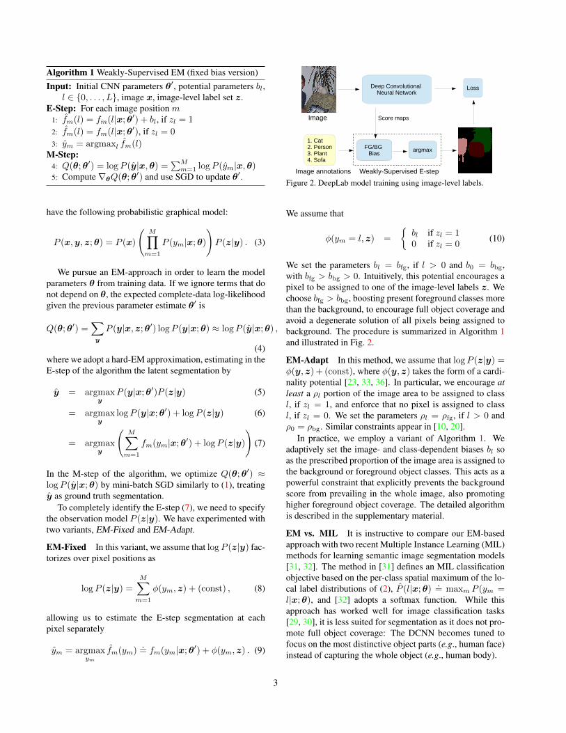
Figure 2. DeepLab model training using image-level labels.
We assume that
φ(ym = l,z) =
{bl if zl = 10 if zl = 0
(10)
We set the parameters bl = bfg, if l > 0 and b0 = bbg,with bfg > bbg > 0. Intuitively, this potential encourages apixel to be assigned to one of the image-level labels z. Wechoose bfg > bbg, boosting present foreground classes morethan the background, to encourage full object coverage andavoid a degenerate solution of all pixels being assigned tobackground. The procedure is summarized in Algorithm 1and illustrated in Fig. 2.
EM-Adapt In this method, we assume that logP (z|y) =φ(y, z) + (const), where φ(y, z) takes the form of a cardi-nality potential [23, 33, 36]. In particular, we encourage atleast a ρl portion of the image area to be assigned to classl, if zl = 1, and enforce that no pixel is assigned to classl, if zl = 0. We set the parameters ρl = ρfg, if l > 0 andρ0 = ρbg. Similar constraints appear in [10, 20].
In practice, we employ a variant of Algorithm 1. Weadaptively set the image- and class-dependent biases bl soas the prescribed proportion of the image area is assigned tothe background or foreground object classes. This acts as apowerful constraint that explicitly prevents the backgroundscore from prevailing in the whole image, also promotinghigher foreground object coverage. The detailed algorithmis described in the supplementary material.
EM vs. MIL It is instructive to compare our EM-basedapproach with two recent Multiple Instance Learning (MIL)methods for learning semantic image segmentation models[31, 32]. The method in [31] defines an MIL classificationobjective based on the per-class spatial maximum of the lo-cal label distributions of (2), P (l|x;θ) .
= maxm P (ym =l|x;θ), and [32] adopts a softmax function. While thisapproach has worked well for image classification tasks[29, 30], it is less suited for segmentation as it does not pro-mote full object coverage: The DCNN becomes tuned tofocus on the most distinctive object parts (e.g., human face)instead of capturing the whole object (e.g., human body).
3

Image
Bbox annotations
Deep Convolutional Neural Network
Segmentation Estimation
DenseCRF
argmax
Loss
Figure 3. DeepLab model training from bounding boxes.
3.3. Bounding Box Annotations
We explore three alternative methods for training oursegmentation model from labeled bounding boxes.
The first Bbox-Rect method amounts to simply consider-ing each pixel within the bounding box as positive examplefor the respective object class. Ambiguities are resolved byassigning pixels that belong to multiple bounding boxes tothe one that has the smallest area.
The bounding boxes fully surround objects but alsocontain background pixels that contaminate the trainingset with false positive examples for the respective objectclasses. To filter out these background pixels, we havealso explored a second Bbox-Seg method in which we per-form automatic foreground/background segmentation. Toperform this segmentation, we use the same CRF as inDeepLab. More specifically, we constrain the center area ofthe bounding box (α% of pixels within the box) to be fore-ground, while we constrain pixels outside the bounding boxto be background. We implement this by appropriately set-ting the unary terms of the CRF. We then infer the labels forpixels in between. We cross-validate the CRF parametersto maximize segmentation accuracy in a small held-out setof fully-annotated images. This approach is similar to thegrabcut method of [34]. Examples of estimated segmenta-tions with the two methods are shown in Fig. 4.
The two methods above, illustrated in Fig. 3, estimatesegmentation maps from the bounding box annotation as apre-processing step, then employ the training procedure ofSec. 3.1, treating these estimated labels as ground-truth.
Our third Bbox-EM-Fixed method is an EM algorithmthat allows us to refine the estimated segmentation mapsthroughout training. The method is a variant of the EM-Fixed algorithm in Sec. 3.2, in which we boost the presentforeground object scores only within the bounding box area.
3.4. Mixed strong and weak annotations
In practice, we often have access to a large number ofweakly image-level annotated images and can only afford toprocure detailed pixel-level annotations for a small fractionof these images. We handle this hybrid training scenario by
Image with Bbox Ground-Truth Bbox-Rect Bbox-Seg
Figure 4. Estimated segmentation from bounding box annotation.
Image Annotations
+
Pixel Annotations
Weakly-Supervised E-step
FG/BGBias
argmax1. Car2. Person3. Horse
Deep Convolutional Neural Network Loss
Deep Convolutional Neural Network
Loss
Score maps
Figure 5. DeepLab model training on a union of full (strong labels)and image-level (weak labels) annotations.
combining the methods presented in the previous sections,as illustrated in Figure 5. In SGD training of our deep CNNmodels, we bundle to each mini-batch a fixed proportionof strongly/weakly annotated images, and employ our EMalgorithm in estimating at each iteration the latent semanticsegmentations for the weakly annotated images.
4. Experimental Evaluation4.1. Experimental Protocol
Datasets The proposed training methods are evaluatedon the PASCAL VOC 2012 segmentation benchmark [13],consisting of 20 foreground object classes and one back-ground class. The segmentation part of the original PAS-CAL VOC 2012 dataset contains 1464 (train), 1449 (val ),and 1456 (test) images for training, validation, and test, re-spectively. We also use the extra annotations provided by[16], resulting in augmented sets of 10, 582 (train aug) and12, 031 (trainval aug) images. We have also experimentedwith the large MS-COCO 2014 dataset [24], which con-tains 123, 287 images in its trainval set. The MS-COCO2014 dataset has 80 foreground object classes and one back-ground class and is also annotated at the pixel level.
The performance is measured in terms of pixelintersection-over-union (IOU) averaged across the 21
4

classes. We first evaluate our proposed methods on the PAS-CAL VOC 2012 val set. We then report our results on theofficial PASCAL VOC 2012 benchmark test set (whose an-notations are not released). We also compare our test setresults with other competing methods.
Reproducibility We have implemented the proposedmethods by extending the excellent Caffe framework [18].We share our source code, configuration files, and trainedmodels that allow reproducing the results in this paperat a companion web site https://bitbucket.org/deeplab/deeplab-public.
Weak annotations In order to simulate the situationswhere only weak annotations are available and to have faircomparisons (e.g., use the same images for all settings), wegenerate the weak annotations from the pixel-level annota-tions. The image-level labels are easily generated by sum-marizing the pixel-level annotations, while the boundingbox annotations are produced by drawing rectangles tightlycontaining each object instance (PASCAL VOC 2012 alsoprovides instance-level annotations) in the dataset.
Network architectures We have experimented with thetwo DCNN architectures of [5], with parameters initializedfrom the VGG-16 ImageNet [11] pretrained model of [35].They differ in the receptive field of view (FOV) size. Wehave found that large FOV (224×224) performs best whenat least some training images are annotated at the pixel level,whereas small FOV (128×128) performs better when onlyimage-level annotations are available. In the main paperwe report the results of the best architecture for each setupand defer the full comparison between the two FOVs to thesupplementary material.
Training We employ our proposed training methods tolearn the DCNN component of the DeepLab-CRF model of[5]. For SGD, we use a mini-batch of 20-30 images and ini-tial learning rate of 0.001 (0.01 for the final classifier layer),multiplying the learning rate by 0.1 after a fixed number ofiterations. We use momentum of 0.9 and a weight decay of0.0005. Fine-tuning our network on PASCAL VOC 2012takes about 12 hours on a NVIDIA Tesla K40 GPU.
Similarly to [5], we decouple the DCNN and Dense CRFtraining stages and learn the CRF parameters by cross val-idation to maximize IOU segmentation accuracy in a held-out set of 100 Pascal val fully-annotated images. We use 10mean-field iterations for Dense CRF inference [19]. Notethat the IOU scores are typically 3-5% worse if we don’tuse the CRF for post-processing of the results.
4.2. Pixel-level annotations
We have first reproduced the results of [5]. Trainingthe DeepLab-CRF model with strong pixel-level annota-tions on PASCAL VOC 2012, we achieve a mean IOU score
Method #Strong #Weak val IOUEM-Fixed (Weak) - 10,582 20.8EM-Adapt (Weak) - 10,582 38.2
EM-Fixed (Semi)
200 10,382 47.6500 10,082 56.9750 9,832 59.8
1,000 9,582 62.01,464 5,000 63.21,464 9,118 64.6
Strong 1,464 - 62.510,582 - 67.6
Table 1. VOC 2012 val performance for varying number of pixel-level (strong) and image-level (weak) annotations (Sec. 4.3).
Method #Strong #Weak test IOUMIL-FCN [31] - 10k 25.7MIL-sppxl [32] - 760k 35.8MIL-obj [32] BING 760k 37.0MIL-seg [32] MCG 760k 40.6
EM-Adapt (Weak) - 12k 39.6
EM-Fixed (Semi) 1.4k 10k 66.22.9k 9k 68.5
Strong [5] 12k - 70.3Table 2. VOC 2012 test performance for varying number of pixel-level (strong) and image-level (weak) annotations (Sec. 4.3).
of 67.6% on val and 70.3% on test ; see method DeepLab-CRF-LargeFOV in [5, Table 1].
4.3. Image-level annotations
Validation results We evaluate our proposed methods intraining the DeepLab-CRF model using image-level weakannotations from the 10,582 PASCAL VOC 2012 train augset, generated as described in Sec. 4.1 above. We reportthe val performance of our two weakly-supervised EM vari-ants described in Sec. 3.2. In the EM-Fixed variant we usebfg = 5 and bbg = 3 as fixed foreground and backgroundbiases. We found the results to be quite sensitive to the dif-ference bfg− bbg but not very sensitive to their absolute val-ues. In the adaptive EM-Adapt variant we constrain at leastρbg = 40% of the image area to be assigned to backgroundand at least ρfg = 20% of the image area to be assigned toforeground (as specified by the weak label set).
We also examine using weak image-level annotationsin addition to a varying number of pixel-level annotations,within the semi-supervised learning scheme of Sec. 3.4.In this Semi setting we employ strong annotations of asubset of PASCAL VOC 2012 train set and use the weakimage-level labels from another non-overlapping subset ofthe train aug set. We perform segmentation inference forthe images that only have image-level labels by means ofEM-Fixed, which we have found to perform better than EM-Adapt in the semi-supervised training setting.
The results are summarized in Table 1. We see that theEM-Adapt algorithm works much better than the EM-Fixedalgorithm when we only have access to image level an-notations, 20.8% vs. 38.2% validation IOU. Using 1,464pixel-level and 9,118 image-level annotations in the EM-Fixed semi-supervised setting significantly improves per-
5

formance, yielding 64.6%. Note that image-level annota-tions are helpful, as training only with the 1,464 pixel-levelannotations only yields 62.5%.
Test results In Table 2 we report our test results. We com-pare the proposed methods with the recent MIL-based ap-proaches of [31, 32], which also report results obtained withimage-level annotations on the VOC benchmark. Our EM-Adapt method yields 39.6%, which improves over MIL-FCN [31] by a large 13.9% margin. As [32] shows, MILcan become more competitive if additional segmentation in-formation is introduced: Using low-level superpixels, MIL-sppxl [32] yields 35.8% and is still inferior to our EM algo-rithm. Only if augmented with BING [7] or MCG [1] canMIL obtain results comparable to ours (MIL-obj: 37.0%,MIL-seg: 40.6%) [32]. Note, however, that both BINGand MCG have been trained with bounding box or pixel-annotated data on the PASCAL train set, and thus bothMIL-obj and MIL-seg indirectly rely on bounding box orpixel-level PASCAL annotations.
The more interesting finding of this experiment is thatincluding very few strongly annotated images in the semi-supervised setting significantly improves the performancecompared to the pure weakly-supervised baseline. Forexample, using 2.9k pixel-level annotations along with9k image-level annotations in the semi-supervised settingyields 68.5%. We would like to highlight that this re-sult surpasses all techniques which are not based on theDCNN+CRF pipeline of [5] (see Table 6), even if trainedwith all available pixel-level annotations.
4.4. Bounding box annotations
Validation results In this experiment, we train theDeepLab-CRF model using bounding box annotations fromthe train aug set. We estimate the training set segmentationsin a pre-processing step using the Bbox-Rect and Bbox-Segmethods described in Sec. 3.3. We assume that we alsohave access to 100 fully-annotated PASCAL VOC 2012 valimages which we have used to cross-validate the value ofthe single Bbox-Seg parameter α (percentage of the cen-ter bounding box area constrained to be foreground). Wevaried α from 20% to 80%, finding that α = 20% maxi-mizes accuracy in terms of IOU in recovering the groundtruth foreground from the bounding box. We also examinethe effect of combining these weak bounding box annota-tions with strong pixel-level annotations, using the semi-supervised learning methods of Sec. 3.4.
The results are summarized in Table 3. When using onlybounding box annotations, we see that Bbox-Seg improvesover Bbox-Rect by 8.1%, and gets within 7.0% of the strongpixel-level annotation result. We observe that combining1,464 strong pixel-level annotations with weak boundingbox annotations yields 65.1%, only 2.5% worse than thestrong pixel-level annotation result. In the semi-supervised
Method #Strong #Box val IOUBbox-Rect (Weak) - 10,582 52.5
Bbox-EM-Fixed (Weak) - 10,582 54.1Bbox-Seg (Weak) - 10,582 60.6Bbox-Rect (Semi) 1,464 9,118 62.1
Bbox-EM-Fixed (Semi) 1,464 9,118 64.8Bbox-Seg (Semi) 1,464 9,118 65.1
Strong 1,464 - 62.510,582 - 67.6
Table 3. VOC 2012 val performance for varying number of pixel-level (strong) and bounding box (weak) annotations (Sec. 4.4).
Method #Strong #Box test IOUBoxSup [9] MCG 10k 64.6BoxSup [9] 1.4k (+MCG) 9k 66.2
Bbox-Rect (Weak) - 12k 54.2Bbox-Seg (Weak) - 12k 62.2Bbox-Seg (Semi) 1.4k 10k 66.6
Bbox-EM-Fixed (Semi) 1.4k 10k 66.6Bbox-Seg (Semi) 2.9k 9k 68.0
Bbox-EM-Fixed (Semi) 2.9k 9k 69.0Strong [5] 12k - 70.3
Table 4. VOC 2012 test performance for varying number of pixel-level (strong) and bounding box (weak) annotations (Sec. 4.4).
learning settings and 1,464 strong annotations, Semi-Bbox-EM-Fixed and Semi-Bbox-Seg perform similarly.
Test results In Table 4 we report our test results. We com-pare the proposed methods with the very recent BoxSup ap-proach of [9], which also uses bounding box annotations onthe VOC 2012 segmentation benchmark. Comparing our al-ternative Bbox-Rect (54.2%) and Bbox-Seg (62.2%) meth-ods, we see that simple foreground-background segmenta-tion provides much better segmentation masks for DCNNtraining than using the raw bounding boxes. BoxSup does2.4% better, however it employs the MCG segmentationproposal mechanism [1], which has been trained with pixel-annotated data on the PASCAL train set; it thus indirectlyrelies on pixel-level annotations.
When we also have access to pixel-level annotated im-ages, our performance improves to 66.6% (1.4k strongannotations) or 69.0% (2.9k strong annotations). In thissemi-supervised setting we outperform BoxSup (66.6% vs.66.2% with 1.4k strong annotations), although we do notuse MCG. Interestingly, Bbox-EM-Fixed improves overBbox-Seg as we add more strong annotations, and it per-forms 1.0% better (69.0% vs. 68.0%) with 2.9k strong an-notations. This shows that the E-step of our EM algorithmcan estimate the object masks better than the foreground-background segmentation pre-processing step when enoughpixel-level annotated images are available.
Comparing with Sec. 4.3, note that 2.9k strong + 9kimage-level annotations yield 68.5% (Table 2), while 2.9kstrong + 9k bounding box annotations yield 69.0% (Ta-ble 3). This finding suggests that bounding box annotationsadd little value over image-level annotations when a suffi-cient number of pixel-level annotations is also available.
6
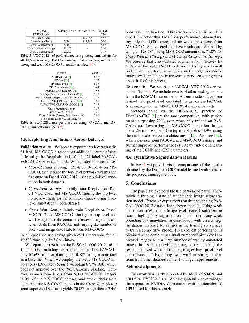
Method #Strong COCO #Weak COCO val IOUPASCAL-only - - 67.6
EM-Fixed (Semi) - 123,287 67.7Cross-Joint (Semi) 5,000 118,287 70.0
Cross-Joint (Strong) 5,000 - 68.7Cross-Pretrain (Strong) 123,287 - 71.0
Cross-Joint (Strong) 123,287 - 71.7Table 5. VOC 2012 val performance using strong annotations forall 10,582 train aug PASCAL images and a varying number ofstrong and weak MS-COCO annotations (Sec. 4.5).
Method test IOUMSRA-CFM [8] 61.8
FCN-8s [25] 62.2Hypercolumn [17] 62.6
TTI-Zoomout-16 [28] 64.4DeepLab-CRF-LargeFOV [5] 70.3
BoxSup (Semi, with weak COCO) [9] 71.0DeepLab-CRF-LargeFOV (Multi-scale net) [5] 71.6
Oxford TVG CRF RNN VOC [42] 72.0Oxford TVG CRF RNN COCO [42] 74.7
Cross-Pretrain (Strong) 72.7Cross-Joint (Strong) 73.0
Cross-Pretrain (Strong, Multi-scale net) 73.6Cross-Joint (Strong, Multi-scale net) 73.9
Table 6. VOC 2012 test performance using PASCAL and MS-COCO annotations (Sec. 4.5).
4.5. Exploiting Annotations Across Datasets
Validation results We present experiments leveraging the81-label MS-COCO dataset as an additional source of datain learning the DeepLab model for the 21-label PASCALVOC 2012 segmentation task. We consider three scenarios:• Cross-Pretrain (Strong) : Pre-train DeepLab on MS-
COCO, then replace the top-level network weights andfine-tune on Pascal VOC 2012, using pixel-level anno-tation in both datasets.
• Cross-Joint (Strong) : Jointly train DeepLab on Pas-cal VOC 2012 and MS-COCO, sharing the top-levelnetwork weights for the common classes, using pixel-level annotation in both datasets.
• Cross-Joint (Semi) : Jointly train DeepLab on PascalVOC 2012 and MS-COCO, sharing the top-level net-work weights for the common classes, using the pixel-level labels from PASCAL and varying the number ofpixel- and image-level labels from MS-COCO.
In all cases we use strong pixel-level annotations for all10,582 train aug PASCAL images.
We report our results on the PASCAL VOC 2012 val inTable 5, also including for comparison our best PASCAL-only 67.6% result exploiting all 10,582 strong annotationsas a baseline. When we employ the weak MS-COCO an-notations (EM-Fixed (Semi) ) we obtain 67.7% IOU, whichdoes not improve over the PASCAL-only baseline. How-ever, using strong labels from 5,000 MS-COCO images(4.0% of the MS-COCO dataset) and weak labels fromthe remaining MS-COCO images in the Cross-Joint (Semi)semi-supervised scenario yields 70.0%, a significant 2.4%
boost over the baseline. This Cross-Joint (Semi) result isalso 1.3% better than the 68.7% performance obtained us-ing only the 5,000 strong and no weak annotations fromMS-COCO. As expected, our best results are obtained byusing all 123,287 strong MS-COCO annotations, 71.0% forCross-Pretrain (Strong) and 71.7% for Cross-Joint (Strong).We observe that cross-dataset augmentation improves by4.1% over the best PASCAL-only result. Using only a smallportion of pixel-level annotations and a large portion ofimage-level annotations in the semi-supervised setting reapsabout half of this benefit.Test results We report our PASCAL VOC 2012 test re-sults in Table 6. We include results of other leading modelsfrom the PASCAL leaderboard. All our models have beentrained with pixel-level annotated images on the PASCALtrainval aug and the MS-COCO 2014 trainval datasets.
Methods based on the DCNN+CRF pipeline ofDeepLab-CRF [5] are the most competitive, with perfor-mance surpassing 70%, even when only trained on PAS-CAL data. Leveraging the MS-COCO annotations bringsabout 2% improvement. Our top model yields 73.9%, usingthe multi-scale network architecture of [5]. Also see [42],which also uses joint PASCAL and MS-COCO training, andfurther improves performance (74.7%) by end-to-end learn-ing of the DCNN and CRF parameters.
4.6. Qualitative Segmentation Results
In Fig. 6 we provide visual comparisons of the resultsobtained by the DeepLab-CRF model learned with some ofthe proposed training methods.
5. ConclusionsThe paper has explored the use of weak or partial anno-
tation in training a state of art semantic image segmenta-tion model. Extensive experiments on the challenging PAS-CAL VOC 2012 dataset have shown that: (1) Using weakannotation solely at the image-level seems insufficient totrain a high-quality segmentation model. (2) Using weakbounding-box annotation in conjunction with careful seg-mentation inference for images in the training set sufficesto train a competitive model. (3) Excellent performance isobtained when combining a small number of pixel-level an-notated images with a large number of weakly annotatedimages in a semi-supervised setting, nearly matching theresults achieved when all training images have pixel-levelannotations. (4) Exploiting extra weak or strong annota-tions from other datasets can lead to large improvements.
Acknowledgments
This work was partly supported by ARO 62250-CS, andNIH 5R01EY022247-03. We also gratefully acknowledgethe support of NVIDIA Corporation with the donation ofGPUs used for this research.
7

Image EM-Adapt (Weak) Bbox-Seg (Weak) EM-Fixed (Semi) Bbox-EM-Fixed (Semi) Cross-Joint (Strong)Figure 6. Qualitative DeepLab-CRF segmentation results on the PASCAL VOC 2012 val set. The last two rows show failure modes.
8
Supplementary Material
We include as appendix: (1) Details of the proposed EM-Adapt algorithm. (2) More experimental evaluations aboutthe effect of the model’s Field-Of-View. (3) More detailedresults of the proposed training methods on PASCAL VOC2012 test set.
A. E-Step with Cardinality Constraints: De-tails of our EM-Adapt Algorithm
Herein we provide more background and a detaileddescription of our EM-Adapt algorithm for weakly-supervised training with image-level annotations.
As a reminder, y is the latent segmentation map, withym ∈ {0, . . . , L} denoting the label at position m ∈{1, . . . ,M}. The image-level annotation is encoded in z,with zl = 1, if the l-th label is present anywhere in the im-age.
We assume that logP (z|y) = φ(y, z) + (const). Weemploy a cardinality potential φ(y, z) which encourages atleast a ρl portion of the image area to be assigned to classl, if zl = 1, and enforce that no pixel is assigned to classl, if zl = 0. We set the parameters ρl = ρfg, if l > 0 andρ0 = ρbg.
While dedicated algorithms exist for optimizing energyfunctions under such cardinality potentials [36, 33, 23], weopt for a simpler alternative that approximately enforcesthese area constraints and works well in practice. Weuse a variant of the EM-Fixed algorithm described in themain paper, updating the segmentations in the E-Step byym = argmaxl fm(l)
.= fm(l|x;θ′) + bl. The key differ-
ence in the EM-Adapt variant is that the biases bl are adap-tively set so as the prescribed proportion of the image areais assigned to the background or foreground object classesthat are present in the image.
When only one label l is present (i.e. zl = 1,∑L
l′=0 zl′ =1), one can easily enforce the constraint that at least ρl ofthe image area is assigned to label l as follows: (1) Set bl′ =0, l′ 6= l. (2) Compute the maximum score at each position,fmaxm = maxLl′=0 fm(l′|x;θ′). (3) Set bl equal to the ρl-th
percentile of the score difference dm = fmaxm −fm(l|x;θ′).
The cost of this algorithm isO(M) (linear w.r.t. the numberof pixels).
When more than one labels are present in the image (i.e.∑Ll′=0 zl′ > 1), we employ the procedure above sequen-
tially for each label that zl > 1 (we first visit the back-ground label, then in random order each of the foregroundlabels which are present in the image). We set bl = −∞,if zl = 0, to suppress the labels that are not present in theimage.
An implementation of this algorithm will become pub-licly available after this paper gets published.
B. Effect of Field-Of-ViewIn this section, we explore the effect of Field-Of-View
(FOV) when training the DeepLab-CRF model with the pro-posed methods in the main paper. Similar to [5], we alsoemploy the ‘atrous’ algorithm [27] in the DeepLab model.The ‘atrous’ algorithm enables us to arbitrary control themodel’s FOV by adjusting the input stride (which is equiv-alent to injecting zeros between filter weights) at the firstfully connected layer of VGG-16 net [35]. Applying a largevalue of input stride increases the effective kernel size, andthus enlarges the model’s FOV (see [5] for details).
Experimental protocol We employ the same experimen-tal protocol as the main paper. Models trained with theproposed training methods and different values of FOV areevaluated on the PASCAL VOC 2012 val set.
EM-Adapt Assuming only image-level labels are avail-able, we first experiment with the EM-Adapt (Weak)method when the value of FOV varies. Specifically, we ex-plore the setting where the kernel size is 3×3 with variousFOV values. The selection of kernel size 3×3 is based onthe discovery by [5]: employing a kernel size of 3×3 at thefirst fully connected layer can attain the same performanceas using the kernel size of 7×7, while being 3.4 times fasterduring training. As shown in Table 7, we find that our pro-posed model can yield the performance of 39.2% with FOV96×96, but the performance degrades by 9% when largeFOV 224×224 is employed. The original DeepLab modelemployed by [5] has a kernel size of 4×4 and input strideof 4. Its performance, shown in the first row of Table 7, issimilar to the performance obtained by using a kernel sizeof 3×3 and input stride of 6. Both cases have the same FOVvalue of 128×128.
Network architectures In the following experiments, wecompare two network architectures trained with the meth-ods proposed in the main paper. The first network is thesame as the one originally employed by [5] (kernel size 4×4and input stride 4, resulting in a FOV size 128×128). Thesecond network we employ has FOV 224×224 (with ker-nel size of 3×3 and an input stride of 12). We refer to thefirst network as ‘DeepLab-CRF with small FOV’, and thesecond network as ‘DeepLab-CRF with large FOV’.
Image-level annotations In Table 8, we experiment withthe cases where weak image-level annotations as well asa varying number of pixel-level annotations are available.Similar to the results in Table 7, the DeepLab-CRF withsmall FOV performs better than that with large FOV whena small amount of supervision is leveraged. Interestingly,when there are more than 750 pixel-level annotations are
9
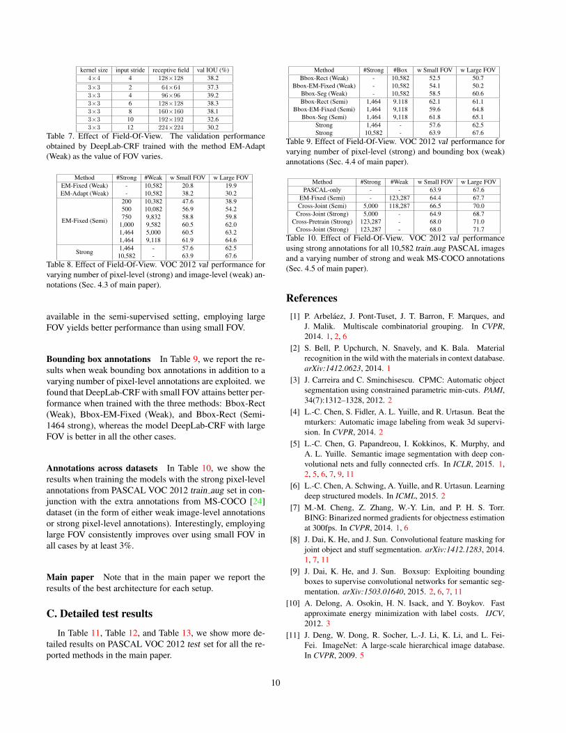
kernel size input stride receptive field val IOU (%)4×4 4 128×128 38.23×3 2 64×64 37.33×3 4 96×96 39.23×3 6 128×128 38.33×3 8 160×160 38.13×3 10 192×192 32.63×3 12 224×224 30.2
Table 7. Effect of Field-Of-View. The validation performanceobtained by DeepLab-CRF trained with the method EM-Adapt(Weak) as the value of FOV varies.
Method #Strong #Weak w Small FOV w Large FOVEM-Fixed (Weak) - 10,582 20.8 19.9EM-Adapt (Weak) - 10,582 38.2 30.2
EM-Fixed (Semi)
200 10,382 47.6 38.9500 10,082 56.9 54.2750 9,832 58.8 59.8
1,000 9,582 60.5 62.01,464 5,000 60.5 63.21,464 9,118 61.9 64.6
Strong 1,464 - 57.6 62.510,582 - 63.9 67.6
Table 8. Effect of Field-Of-View. VOC 2012 val performance forvarying number of pixel-level (strong) and image-level (weak) an-notations (Sec. 4.3 of main paper).
available in the semi-supervised setting, employing largeFOV yields better performance than using small FOV.
Bounding box annotations In Table 9, we report the re-sults when weak bounding box annotations in addition to avarying number of pixel-level annotations are exploited. wefound that DeepLab-CRF with small FOV attains better per-formance when trained with the three methods: Bbox-Rect(Weak), Bbox-EM-Fixed (Weak), and Bbox-Rect (Semi-1464 strong), whereas the model DeepLab-CRF with largeFOV is better in all the other cases.
Annotations across datasets In Table 10, we show theresults when training the models with the strong pixel-levelannotations from PASCAL VOC 2012 train aug set in con-junction with the extra annotations from MS-COCO [24]dataset (in the form of either weak image-level annotationsor strong pixel-level annotations). Interestingly, employinglarge FOV consistently improves over using small FOV inall cases by at least 3%.
Main paper Note that in the main paper we report theresults of the best architecture for each setup.
C. Detailed test results
In Table 11, Table 12, and Table 13, we show more de-tailed results on PASCAL VOC 2012 test set for all the re-ported methods in the main paper.
Method #Strong #Box w Small FOV w Large FOVBbox-Rect (Weak) - 10,582 52.5 50.7
Bbox-EM-Fixed (Weak) - 10,582 54.1 50.2Bbox-Seg (Weak) - 10,582 58.5 60.6Bbox-Rect (Semi) 1,464 9.118 62.1 61.1
Bbox-EM-Fixed (Semi) 1,464 9,118 59.6 64.8Bbox-Seg (Semi) 1,464 9,118 61.8 65.1
Strong 1,464 - 57.6 62.5Strong 10,582 - 63.9 67.6
Table 9. Effect of Field-Of-View. VOC 2012 val performance forvarying number of pixel-level (strong) and bounding box (weak)annotations (Sec. 4.4 of main paper).
Method #Strong #Weak w Small FOV w Large FOVPASCAL-only - - 63.9 67.6
EM-Fixed (Semi) - 123,287 64.4 67.7Cross-Joint (Semi) 5,000 118,287 66.5 70.0
Cross-Joint (Strong) 5,000 - 64.9 68.7Cross-Pretrain (Strong) 123,287 - 68.0 71.0
Cross-Joint (Strong) 123,287 - 68.0 71.7Table 10. Effect of Field-Of-View. VOC 2012 val performanceusing strong annotations for all 10,582 train aug PASCAL imagesand a varying number of strong and weak MS-COCO annotations(Sec. 4.5 of main paper).
References[1] P. Arbelaez, J. Pont-Tuset, J. T. Barron, F. Marques, and
J. Malik. Multiscale combinatorial grouping. In CVPR,2014. 1, 2, 6
[2] S. Bell, P. Upchurch, N. Snavely, and K. Bala. Materialrecognition in the wild with the materials in context database.arXiv:1412.0623, 2014. 1
[3] J. Carreira and C. Sminchisescu. CPMC: Automatic objectsegmentation using constrained parametric min-cuts. PAMI,34(7):1312–1328, 2012. 2
[4] L.-C. Chen, S. Fidler, A. L. Yuille, and R. Urtasun. Beat themturkers: Automatic image labeling from weak 3d supervi-sion. In CVPR, 2014. 2
[5] L.-C. Chen, G. Papandreou, I. Kokkinos, K. Murphy, andA. L. Yuille. Semantic image segmentation with deep con-volutional nets and fully connected crfs. In ICLR, 2015. 1,2, 5, 6, 7, 9, 11
[6] L.-C. Chen, A. Schwing, A. Yuille, and R. Urtasun. Learningdeep structured models. In ICML, 2015. 2
[7] M.-M. Cheng, Z. Zhang, W.-Y. Lin, and P. H. S. Torr.BING: Binarized normed gradients for objectness estimationat 300fps. In CVPR, 2014. 1, 6
[8] J. Dai, K. He, and J. Sun. Convolutional feature masking forjoint object and stuff segmentation. arXiv:1412.1283, 2014.1, 7, 11
[9] J. Dai, K. He, and J. Sun. Boxsup: Exploiting boundingboxes to supervise convolutional networks for semantic seg-mentation. arXiv:1503.01640, 2015. 2, 6, 7, 11
[10] A. Delong, A. Osokin, H. N. Isack, and Y. Boykov. Fastapproximate energy minimization with label costs. IJCV,2012. 3
[11] J. Deng, W. Dong, R. Socher, L.-J. Li, K. Li, and L. Fei-Fei. ImageNet: A large-scale hierarchical image database.In CVPR, 2009. 5
10

Method bkg aero bike bird boat bottle bus car cat chair cow table dog horse mbike person plant sheep sofa train tv meanMIL-FCN [31] - - - - - - - - - - - - - - - - - - - - - 25.7MIL-sppxl [32] 74.7 38.8 19.8 27.5 21.7 32.8 40.0 50.1 47.1 7.2 44.8 15.8 49.4 47.3 36.6 36.4 24.3 44.5 21.0 31.5 41.3 35.8MIL-obj [32] 76.2 42.8 20.9 29.6 25.9 38.5 40.6 51.7 49.0 9.1 43.5 16.2 50.1 46.0 35.8 38.0 22.1 44.5 22.4 30.8 43.0 37.0MIL-seg [32] 78.7 48.0 21.2 31.1 28.4 35.1 51.4 55.5 52.8 7.8 56.2 19.9 53.8 50.3 40.0 38.6 27.8 51.8 24.7 33.3 46.3 40.6
EM-Adapt (Weak) 76.3 37.1 21.9 41.6 26.1 38.5 50.8 44.9 48.9 16.7 40.8 29.4 47.1 45.8 54.8 28.2 30.0 44.0 29.2 34.3 46.0 39.6EM-Fixed (Semi-1464 strong) 91.3 78.9 37.3 81.4 57.1 57.7 83.5 77.5 77.6 22.5 70.3 56.1 72.2 74.3 80.7 72.4 42.0 81.3 43.1 72.5 60.7 66.2EM-Fixed (Semi-2913 strong) 92.0 81.6 42.9 80.5 59.2 60.8 85.5 78.7 77.3 26.9 75.2 57.6 74.0 74.2 82.1 73.1 52.4 84.3 43.8 75.1 61.9 68.5
Table 11. VOC 2012 test performance for varying number of pixel-level (strong) and image-level (weak) annotations (Sec. 4.3 of mainpaper). Links to the PASCAL evaluation server are included in the PDF.
Method bkg aero bike bird boat bottle bus car cat chair cow table dog horse mbike person plant sheep sofa train tv meanBoxSup-box [9] - 80.3 31.3 82.1 47.4 62.6 75.4 75.0 74.5 24.5 68.3 56.4 73.7 69.4 75.2 75.1 47.4 70.8 45.7 71.1 58.8 64.6BoxSup-semi [9] - 82.0 33.6 74.0 55.8 57.5 81.0 74.6 80.7 27.6 70.9 50.4 71.6 70.8 78.2 76.9 53.5 72.6 50.1 72.3 64.4 66.2
Bbox-Rect (Weak) 82.9 43.6 22.5 50.5 45.0 62.5 76.0 66.5 61.2 25.3 55.8 52.1 56.6 48.1 60.1 58.2 49.5 58.3 40.7 62.3 61.1 54.2Bbox-Seg (Weak) 89.2 64.4 27.3 67.6 55.1 64.0 81.6 70.5 76.0 24.1 63.8 58.2 72.1 59.8 73.5 71.4 47.4 76.0 44.2 68.9 50.9 62.2
Bbox-Seg (Semi-1464 strong) 91.3 75.3 29.9 74.4 59.8 64.6 84.3 76.2 79.0 27.9 69.1 56.5 73.8 66.7 78.8 76.0 51.8 80.8 47.5 73.6 60.5 66.6Bbox-EM-Fixed (Semi-1464 strong) 91.9 78.3 36.5 86.2 53.8 62.5 81.2 80.0 83.2 22.8 68.9 46.7 78.1 72.0 82.2 78.5 44.5 81.1 36.4 74.6 60.2 66.6
Bbox-Seg (Semi-2913 strong) 92.0 76.4 34.1 79.2 61.0 65.6 85.0 76.9 81.5 28.5 69.3 58.0 75.5 69.8 79.3 76.9 54.0 81.4 46.9 73.6 62.9 68.0Bbox-EM-Fixed (Semi-2913 strong) 92.5 80.4 41.6 84.6 59.0 64.7 84.6 79.6 83.5 26.3 71.2 52.9 78.3 72.3 83.3 79.1 51.7 82.1 42.5 75.0 63.4 69.0
Table 12. VOC 2012 test performance for varying number of pixel-level (strong) and bounding box (weak) annotations (Sec. 4.4 of mainpaper). Links to the PASCAL evaluation server are included in the PDF.
Method bkg aero bike bird boat bottle bus car cat chair cow table dog horse mbike person plant sheep sofa train tv meanMSRA-CFM [8] - 75.7 26.7 69.5 48.8 65.6 81.0 69.2 73.3 30.0 68.7 51.5 69.1 68.1 71.7 67.5 50.4 66.5 44.4 58.9 53.5 61.8
FCN-8s [25] - 76.8 34.2 68.9 49.4 60.3 75.3 74.7 77.6 21.4 62.5 46.8 71.8 63.9 76.5 73.9 45.2 72.4 37.4 70.9 55.1 62.2Hypercolumn [17] - 68.7 33.5 69.8 51.3 70.2 81.1 71.9 74.9 23.9 60.6 46.9 72.1 68.3 74.5 72.9 52.6 64.4 45.4 64.9 57.4 62.6
TTI-Zoomout-16 [28] 89.8 81.9 35.1 78.2 57.4 56.5 80.5 74.0 79.8 22.4 69.6 53.7 74.0 76.0 76.6 68.8 44.3 70.2 40.2 68.9 55.3 64.4CRF RNN [42] - 80.9 34.0 72.9 52.6 62.5 79.8 76.3 79.9 23.6 67.7 51.8 74.8 69.9 76.9 76.9 49.0 74.7 42.7 72.1 59.6 65.2
DeepLab-CRF-LargeFOV [5] 92.6 83.5 36.6 82.5 62.3 66.5 85.4 78.5 83.7 30.4 72.9 60.4 78.5 75.5 82.1 79.7 58.2 82.0 48.8 73.7 63.3 70.3Oxford TVG CRF RNN [42] - 85.5 36.7 77.2 62.9 66.7 85.9 78.1 82.5 30.1 74.8 59.2 77.3 75.0 82.8 79.7 59.8 78.3 50.0 76.9 65.7 70.4
BoxSup-semi-coco [9] - 86.4 35.5 79.7 65.2 65.2 84.3 78.5 83.7 30.5 76.2 62.6 79.3 76.1 82.1 81.3 57.0 78.2 55.0 72.5 68.1 71.0DeepLab-MSc-CRF-LargeFOV [5] 93.1 84.4 54.5 81.5 63.6 65.9 85.1 79.1 83.4 30.7 74.1 59.8 79.0 76.1 83.2 80.8 59.7 82.2 50.4 73.1 63.7 71.6
Oxford TVG CRF RNN COCO [42] - 90.4 55.3 88.7 68.4 69.8 88.3 82.4 85.1 32.6 78.5 64.4 79.6 81.9 86.4 81.8 58.6 82.4 53.5 77.4 70.1 74.7Cross-Pretrain (Strong) 93.4 89.1 38.3 88.1 63.3 69.7 87.1 83.1 85.0 29.3 76.5 56.5 79.8 77.9 85.8 82.4 57.4 84.3 54.9 80.5 64.1 72.7
Cross-Joint (Strong) 93.3 88.5 35.9 88.5 62.3 68.0 87.0 81.0 86.8 32.2 80.8 60.4 81.1 81.1 83.5 81.7 55.1 84.6 57.2 75.7 67.2 73.0Cross-Pretrain (Strong, Multi-scale net) 93.8 88.7 53.1 87.7 64.4 69.5 85.9 81.6 85.3 31.0 76.4 62.0 79.8 77.3 84.6 83.2 59.1 85.5 55.9 76.5 64.3 73.6
Cross-Joint (Strong, Multi-scale net) 93.7 89.2 46.7 88.5 63.5 68.4 87.0 81.2 86.3 32.6 80.7 62.4 81.0 81.3 84.3 82.1 56.2 84.6 58.3 76.2 67.2 73.9
Table 13. VOC 2012 test performance using strong PASCAL and strong MS-COCO annotations (Sec. 4.5 of main paper). Links to thePASCAL evaluation server are included in the PDF.
[12] P. Duygulu, K. Barnard, J. F. de Freitas, and D. A. Forsyth.Object recognition as machine translation: Learning a lexi-con for a fixed image vocabulary. In ECCV, 2002. 2
[13] M. Everingham, S. M. A. Eslami, L. V. Gool, C. K. I.Williams, J. Winn, and A. Zisserma. The pascal visual objectclasses challenge a retrospective. IJCV, 2014. 1, 4
[14] C. Farabet, C. Couprie, L. Najman, and Y. LeCun. Learninghierarchical features for scene labeling. PAMI, 2013. 1
[15] M. Guillaumin, D. Kuttel, and V. Ferrari. Imagenetauto-annotation with segmentation propagation. IJCV,110(3):328–348, 2014. 2
[16] B. Hariharan, P. Arbelaez, L. Bourdev, S. Maji, and J. Malik.Semantic contours from inverse detectors. In ICCV, 2011. 4
[17] B. Hariharan, P. Arbelaez, R. Girshick, and J. Malik. Hyper-columns for object segmentation and fine-grained localiza-tion. arXiv:1411.5752, 2014. 7, 11
[18] Y. Jia et al. Caffe: Convolutional architecture for fast featureembedding. arXiv:1408.5093, 2014. 5
[19] P. Krahenbuhl and V. Koltun. Efficient inference in fullyconnected crfs with gaussian edge potentials. In NIPS, 2011.1, 2, 5
[20] H. Kuck and N. de Freitas. Learning about individuals fromgroup statistics. In UAI, 2005. 3
[21] M. P. Kumar, H. Turki, D. Preston, and D. Koller. Learn-ing specific-class segmentation from diverse data. In ICCV,2011. 2
[22] V. Lempitsky, P. Kohli, C. Rother, and T. Sharp. Image seg-mentation with a bounding box prior. In ICCV, 2009. 2
[23] Y. Li and R. Zemel. High order regularization for semi-supervised learning of structured output problems. In ICML,2014. 3, 9
[24] T.-Y. Lin et al. Microsoft COCO: Common objects in con-text. In ECCV, 2014. 1, 4, 10
[25] J. Long, E. Shelhamer, and T. Darrell. Fully convolutionalnetworks for semantic segmentation. arXiv:1411.4038,2014. 1, 7, 11
[26] W.-L. Lu, J.-A. Ting, J. J. Little, and K. P. Murphy. Learningto track and identify players from broadcast sports videos.PAMI, 2013. 2
[27] S. Mallat. A Wavelet Tour of Signal Processing. Acad. Press,2 edition, 1999. 9
[28] M. Mostajabi, P. Yadollahpour, and G. Shakhnarovich.Feedforward semantic segmentation with zoom-out features.arXiv:1412.0774, 2014. 1, 7, 11
[29] M. Oquab, L. Bottou, I. Laptev, and J. Sivic. Weakly super-vised object recognition with convolutional neural networks.In NIPS, 2014. 3
11
[30] G. Papandreou, I. Kokkinos, and P.-A. Savalle. Untanglinglocal and global deformations in deep convolutional net-works for image classification and sliding window detection.arXiv:1412.0296, 2014. 3
[31] D. Pathak, E. Shelhamer, J. Long, and T. Darrell.Fully convolutional multi-class multiple instance learning.arXiv:1412.7144, 2014. 2, 3, 5, 6, 11
[32] P. Pinheiro and R. Collobert. From image-level to pixel-levellabeling with convolutional networks. In CVPR, 2015. 1, 2,3, 5, 6, 11
[33] P. Pletscher and P. Kohli. Learning low-order models forenforcing high-order statistics. In AISTATS, 2012. 3, 9
[34] C. Rother, V. Kolmogorov, and A. Blake. GrabCut: Inter-active foreground extraction using iterated graph cuts. InSIGGRAPH, 2004. 2, 4
[35] K. Simonyan and A. Zisserman. Very deep con-volutional networks for large-scale image recognition.arXiv:1409.1556, 2014. 5, 9
[36] D. Tarlow, K. Swersky, R. S. Zemel, R. P. Adams, and B. J.Frey. Fast exact inference for recursive cardinality models.In UAI, 2012. 3, 9
[37] J. Verbeek and B. Triggs. Region classification with markovfield aspect models. In CVPR, 2007. 2
[38] A. Vezhnevets, V. Ferrari, and J. M. Buhmann. Weakly su-pervised structured output learning for semantic segmenta-tion. In CVPR, 2012. 2
[39] W. Xia, C. Domokos, J. Dong, L.-F. Cheong, and S. Yan. Se-mantic segmentation without annotating segments. In ICCV,2013. 2
[40] J. Xu, A. G. Schwing, and R. Urtasun. Tell me what you seeand I will show you where it is. In CVPR, 2014. 2
[41] J. Xu, A. G. Schwing, and R. Urtasun. Learning to segmentunder various forms of weak supervision. In CVPR, 2015. 2
[42] S. Zheng, S. Jayasumana, B. Romera-Paredes, V. Vineet,Z. Su, D. Du, C. Huang, and P. Torr. Conditional randomfields as recurrent neural networks. arXiv:1502.03240, 2015.1, 2, 7, 11
[43] J. Zhu, J. Mao, and A. L. Yuille. Learning from weakly su-pervised data by the expectation loss svm (e-svm) algorithm.In NIPS, 2014. 2
12